Introduction to Wireless and Cellular CommunicationIntroduction to CDMAProf. David Koilpillai

Department of Electrical EngineeringIndian Institute of Technology, Madras

Lecture - 46Features of CDMA 2000 and WCDMA

Good morning, we begin lecture 46. This is the last 2 lectures or probably 3 lectures on

CDMA. Some very important concepts that we want to cover: one is the concept of the rake

receiver and how does CDMA also work; the method by which it achieve the performance in

a multi user environment.

(Refer Slide Time: 00:34)

There are lots of similarities. So, the framework that we developed for the multipath will also

be useful in our understanding of the multi user. So, we will try to keep both those they are

not distinct keep them as 2 pieces that are tightly interconnected.

(Refer Slide Time: 01:03)

So, by way of a quick review of yesterday’s concepts. One of the things that we have studied

is the role of m sequences, m sequences are used quite extensively for scrambling we have

seen that as a you know several different places, where it is used for scrambling and. So, it is

useful for us to know it is properties. The key properties that we leverage is are the following

that if I had - basically the shift property, if I add a m sequence with a shifted version of itself.

So, basically shift cyclically shifted by n times. So, this is the notation that we have been

using for the following. So, this basically stands for b of n plus k mod Q, where Q is the

length of the m sequence and we said that this is equal to another shifted version and we will

actually see that this property plays an important role in today’s discussion.

So, this is one of the properties of the m sequences, another very useful property of the m

sequence is the cyclic correlation; R x of k defined as 1 over Q summation L equal to 0

through Q minus 1, x of L x star of L minus k mod Q and we showed that this is minus 1 by

Q using the shift property and again these are linked and useful for us to remember because

this property comes into play in several places. Maybe it is good for us to mention right here

that we have used both the representations of m sequences. For example, this property is

based on the binary representation because you are doing modulo 2. This property the way

we have written it is based on the bipolar; so a 0 mapping to a 1, a 1 mapping to a minus 1.

So, in other words x of i is equal to 1 minus 2 times the corresponding bit value ok.

So, we have used both the representations. So, please all always before you apply something

it is I am I working in binary or I am working in bipolar, that is an important part to keep in

mind I meant to ask a question we use the word scrambling is scrambling different from

encryption. I see several (Refer Time: 03:52) what is the difference scrambling versus

encryption. The point that is mentioned of scrambling means that the order of the bits has

been changed, in our notation particularly the way it is defined in CDMA 2000 scrambling is

slightly different. Basically you do a modulo 2 addition with a another sequence. So,

basically you have the original sequence and a modulo 2 addition.

So, let me just write that down. So, if I have a what I call a message sequence in the case of

CDMA 2000 it would be 1.2288 mega chips per second, then to be the scrambling operation

actually turns out to be a mod, this is also at 1.2288 mega chips per second and comes out a

modified sequence which is also at the same rate. So, we can make the following statements

that scrambling is a bit level operation you input in 1 bit you get another bit. So, we do use

the word scrambling to change the order also, but in the context of the CDMA systems the

scrambling that we are talking. Scrambling we in our context is to make the data look

random.

So, a it is more than just the shuffling of the order of the bits it is actually doing a modulo to

addition. So, it is a bit level operation, notice the input and output rates are the same. So, it is

very important to note that it does not increase bandwidth. So, scrambling does not increase

bandwidth. Now the purpose of scrambling is to make the data look random at the physical

layer, it is a scrambling is a physical layer phenomenon encryption on the other hand is not

necessarily a physical layer, from it is you basically want to be able to hide your data. So, that

somebody else cannot receive it.

So, usually encryption is done at the higher layers, it is usually done at the application layer.

Whatever is the data that you get you will you want to represent it in some other way. So,

encryption also does not increase bandwidth, usually our algorithms if you give a 128 bit

sequence, will produce for you an encrypted 128 bit sequence. So, encryption also does not

increase bandwidth, but keep in mind it has a very different purpose than the scrambling that

we have done. Because scrambling undoing the scrambling should be very easy because once

you know the m sequence. So, the reverse operation is easy that is for scrambling of yes

reverse operation is very easy if you know the m sequence you just do the whereas for the

encryption you want the reverse operation to be as hard as possible ok.

So, there is a fundamental difference reverse operation, you want to make it as difficult as

possible. So, that un unwanted user may not have access to the information. So, these 2 are

similar. Now the only bandwidth expanding operation that we have in the CDMA system

bandwidth expansion comes only through the spreading process.

Student: Sir even in a encryption you only separation to be difficult for the 1 who does not

know the key and for the 1 who knows the key or in this case the spreading sequence m

sequence (Refer Time: 07:38).

So, in the basically it is the reverse operation is difficult for every one other than the desired

user that is correct yes.

Student: (Refer Time: 07:45) same with the m same with the m sequence also (Refer Time:

07:50).

So, m sequence is as you know it is very easy to find out once you know the field shift

feedback tabs, usually in the case of CDMA the m sequence is actually published it is a it is

in the public domain say. So, basically it is a matter of waiting for you to synchronize with m

sequence. So, the scrambling part is somebody something that anybody can do the d

scrambling part can do, but the encryption is done at a higher layer it is done with some

secret information all the information about the encryption algorithms, usually are not

published. So, there are some secret information. So, again to that extent the scrambling

operation has a very definite goal it wants to make the data look random make it look like

white noise. So, sometimes you may have a string of zeroes you may not want that to come as

a string of zeroes in your sequence.

So, scrambling will make sure that you know any string of zeroes get sort of modified. So,

like that the bit level operation of scrambling makes the data look random. Encryption the

intent is not that at all I mean it has a very specific thing of hiding the user information. So,

bandwidth expansion comes primarily and or solely from the spreading operation. So, there is

spreading there is encryption there is scrambling encryption is something that we have not

touched upon it is a basically it is a part of digital communications that happens at a higher

layer what we have been focusing on has been bandwidth expansion through spreading and

we also been looking at scrambling as a way to randomize the data also pro protect us against

some elements of multipath as well ok.

(Refer Slide Time: 09:48)

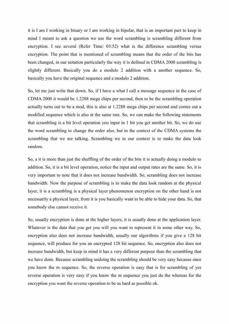
Let me just if I gave you a irreducible polynomial I tell you that the following is an

irreducible polynomial, 1 plus x plus x squared plus x for power 5 plus x power 6 and I ask

you to generate and it and tell you that it is a maximal length sequence, you should be able to

connect the feedback taps and actually generate 1 period of the sequence. So, this is a sixth

order polynomial. So, if I want to implement it I must have 6 shift registers I can rewrite the

polynomial in terms of delays and please make sure the correction connections are done

correctly otherwise you will not it may not be a maximal length sequence.

So, the output of the first delay is taken these all modulo 2 additions that you have do is by it

is in the binary representation. Second delay is also taken. So, this is delay delay delay delay

delay then I do not need the output of the third delay, fourth delay need the output of the fifth

delay and the output of the sixth delay, this output is the sequence and this tap actually is the

feedback tap that is. So, 1 equal to x plus x squared plus x 5 plus x 6 is the feedback

connections, you can start with any starting state does not matter and you will basically the

sequence will repeat itself.

So, we should get a to power 6 minus 1 in this case 63 sequence, do not do it by hand it is not

I just want you to make sure that you are able to do that. Another point to reinforce from our

discussion yesterday.

(Refer Slide Time: 11:56)

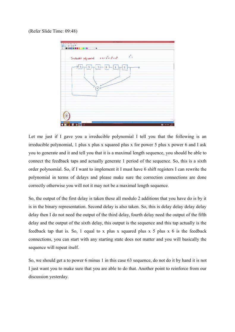
Difference between CDMA 2000 and wideband CDMA, the chip rate that we were using is

1.2288 mega chips per second, all channels must have this chip rate the occupied bandwidth

of the CDMA 2000 signal is 1.25 megahertz. So, that is how the channelization is done, the

channel that is of most interest to us is a traffic channel, traffic channel originally designed to

be primarily voice. So, it takes in voice encoded voice or compressed voice a 9.6 kilobits per

second and then as you know it does the rest of the processing, the first stage is the

convolutional coding that it does makes it 19.2 kilobits per second - this is the convolutional

coding.

The next step is the spreading Q is equal to 64 is the spreading factor, that we use and it is

one of the codes of from the Walsh 64 length Walsh Hadamard sequences, and this basically

gives us this is the spreading operation. So, there are 2 stages of bandwidth expansion; coding

also expands the bandwidth spreading expands the bandwidth, both and eventually we get to

1.2288 mega chips per second. If somebody wanted more than 9.6 kilobits per second you

would have to give them multiple spreading codes.

Now, on the other hand wideband CDMA has the has a chip rate which is 3.84 mega chips

per second in an occupied bandwidth of 5 megahertz roughly 4 times the bandwidth of the

CDMA 2000 system 4 times the bandwidth should approximately scale to 4 times the

capacity because that is how the systems are designed. So, in this case the spreading factors

are not from are from the Walsh Hadamard family, but from they are from the OVSF set.

So, OVSF set OVSF L comma n represents the nth code of length L where length L can be

either 2 squared or 2 cubed 2 power 4 dot dot dot in wideband CDMA there is a provision to

vary the spreading factor all the way from 4 to 512. So, you know very high spreading factors

to very low spreading factors, but most commonly 512 is not used. So, it is from 0 to 2 4 to

256, but still it has larger spread and it is 3.84 mega chips per second in 5 megahertz. We also

made an observation if you remember that CDMA 2000 does power control at the rate of 800

hertz or 800 times per second, it tells you to go up or down it tells the users to go up or down.

So, in other words it is 800 adjustments per second ok.

Now, here is a question which will indicate you know I want you to have an intuitive feel for

CDMA systems and if you can answer this question, it will be very helpful for the entire

class. So, the question is the observation is the following wideband CDMA does power

control at the rate of 1500 times per second the question is why? Why did it have to do more

than the number of times as CDMA as CDMA 2000, can you think of any reasons? There are

at least 2 very important reasons.

Student: More number of users.

Very good first answer was more number of users because it is a 5 megahertz system you

have more codes available more users are present and if somebody if one of the users is using

excess power, then it will affect lots of users. So, you do not want to take a chance you want

to control that. So, first one is the fact that it is wider bandwidth which means more users and

if one of the users is using excess power it is going to affect a lot more people. So, you want

to have a tighter control. One more reason - this will really tell me that you have fully

understood the CDMA part, if the answer is there on the slide.

Student: (Refer Time: 16:54).

Answer is there on the slide what protects you against a multi user interference.

Student: Spreading.

It is just spreading (Refer Time: 17:04).

Student: (Refer Time: 17:07).

In wideband CDMA.

Student: (Refer Time: 17:08).

There are some users who are running at.

Student: (Refer Time: 17:10).

Spreading fact of 4 they do not have much protection why are they running why are they

using spreading factor of 4 because they have lots of data to send. Now if they have less

protection against multi user interference. So, if there is somebody else who is transmitting

with more power, they can actually kill these users. So, you want to control these users.

So, typically in wideband CDMA system somebody with spreading factor 4, because he does

not have much processing gain will be transmitting with higher power than the one who is

using spreading factor 256 is that correct does that make sense? Because he is got more data

to send you have to use more power to get your data across right and if its so, one is if

somebody else transmits with more power you do not have much protection, because you are

using only spreading factor of 4.

Now, the second use you use more power, but already you are at higher power if you use

more power than you need you are going to affect others as well. So, the fact that you have

more users the fact that you have some users with less spreading factor who are transmitting

at high power it is a interaction. So, a second one second reason would be maybe just to say

that yes there are low spreading factor users, and they actually are complicate the system

because the they have less protection against interference because their spreading factor is

low, but they also are transmitting with higher power - less protection against interference.

So, again once you understand CDMA at an intuitive level, it starts to become very very

interesting. So, they are transmitted in low spreading factors they are transmitting with high

power higher power, transmitting with higher power. So, you want to control them more

tightly with higher power ok.

So, everything that you have studied in additional communications is embedded here it is just

that you know just had to make sure you catch those interesting elements.

(Refer Slide Time: 19:27)

Yesterday we did the OVSF we will not repeat that, except to go through and fill in the last

column if you had assigned 128 comma 127 instead of 128 comma 2 you should get the

following codes does not affect the length 256 codes does not affect the 128 codes

But it starts to affect the lower value and does not affect the 64 as well, because if you go

through and do that, but it does affect the lower spreading factor codes 30 and only 2 are

available from the spreading factor 4, Because this particular code 128 comma 127 comes

from a different parent - from the if you go back in the OVSF 3 and. So, it does not affect the

number of successors, but it affects the number of earlier codes or predecessor codes and this

is an indication that if you do not do your code assignment properly, you actually can affect

your capacity. So, there is some concept or understanding of something called code

reassignment. For optimization of the performance, you can do a code reassignment and say

no instead of during spreading factor 1 to code number 127 you know start using code

number 2 and user says it does not matter to me I can use any code and it is not a problem.

So, once you do that, you have more codes available in the system. So, there is an interesting

optimization that can be done if you what you do called pack your codes so that you

minimize the number of predecessors. So, that way you have more flexibility in the

assignment of codes it is an interesting one I am sure you see the pattern ok.

(Refer Slide Time: 21:21)

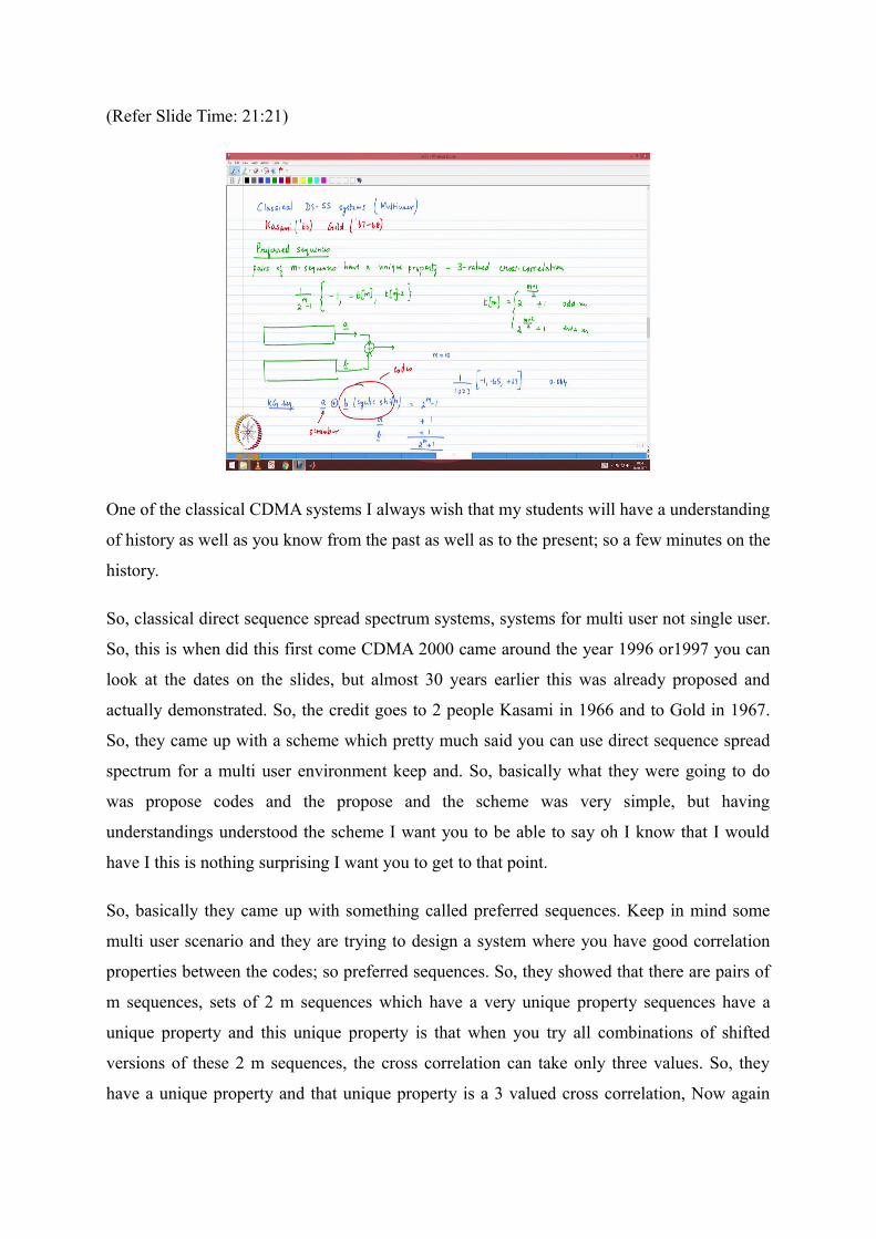
One of the classical CDMA systems I always wish that my students will have a understanding

of history as well as you know from the past as well as to the present; so a few minutes on the

history.

So, classical direct sequence spread spectrum systems, systems for multi user not single user.

So, this is when did this first come CDMA 2000 came around the year 1996 or1997 you can

look at the dates on the slides, but almost 30 years earlier this was already proposed and

actually demonstrated. So, the credit goes to 2 people Kasami in 1966 and to Gold in 1967.

So, they came up with a scheme which pretty much said you can use direct sequence spread

spectrum for a multi user environment keep and. So, basically what they were going to do

was propose codes and the propose and the scheme was very simple, but having

understandings understood the scheme I want you to be able to say oh I know that I would

have I this is nothing surprising I want you to get to that point.

So, basically they came up with something called preferred sequences. Keep in mind some

multi user scenario and they are trying to design a system where you have good correlation

properties between the codes; so preferred sequences. So, they showed that there are pairs of

m sequences, sets of 2 m sequences which have a very unique property sequences have a

unique property and this unique property is that when you try all combinations of shifted

versions of these 2 m sequences, the cross correlation can take only three values. So, they

have a unique property and that unique property is a 3 valued cross correlation, Now again

how this comes about and you know they how to identify these sequences is not the important

point, that they showed that such pairs exist and the cross correlation turns out to be the

following.

So, if they are length m sequences the length will be 2 to the power of m minus 1. So, that is

your scale factor the cross correlation can be minus 1; that means, these 2 codes are perfectly

orthogonal to each other as close to perfectly orthogonal or it can have a value which is given

by a function t of m I will define t of m in a moment or it can be t of m minus 2. These are the

three values and they showed that this function t of m is 2 power m plus 1 divided by 2 plus 1

if it is if m is odd and it is equal to 2 power m plus 2 divided by 2 plus 1 for even m this is

what was proposed and they basically said that they would generate.

If you have 2 m sequences one is the generation of m sequence number 1 a, this is the second

m sequence this is b and basically they said using this combination of preferred sequences

that they would generate for you a set of codes that will give you good performance and this

was one of the you know absolutely remarkable results because all it said was you know you

have now a large family of codes which have good cross correlation basically just so that you

get a feel for the numbers if you take m equal to 10. So, it will be 1 by 1023 what are these

correlation values? It is minus 1 it is plus 60 minus 65 or plus 63, ok.

So, 65 by 1023 is 0.064 this is a reasonably low cross correlation. So, what we are saying is

that go Kasami and gold came up with a set of sequences which guaranteed you that the cross

correlation is going to be good, which means that you could use them for their. So, basically

now we look at and say well you know how good was this result and you know some insight

into that. So, first we need to know how these gold Kasami gold sequences were generated.

So, kg sequences; kg sequences where they said take a and x or it with b with all possible

cyclic shifts and of course, you can get 2 power m minus 1 cyclic shifts ok.

So, this basically will give you 2 power m minus 1 combinations, basically a is a sequence of

length 2 m minus 1, b is a sequence of length 2 m minus 1 if they saying try all the cyclic

combinations then they said you can also take a as one of the sequences. So, it becomes 1

plus 1 and then you can take b also plus 1. So, it is 2 power m plus 1 and the guarantee was

this does not have the same confusion between multipath and multi user and. So, 2 things that

just like to quickly work with you one is first of all the property, you know why is it that if I

have just 2 sequences and then I will do cyclic shifts how is the property preserved ok.

Let us do that because once you do that then you appreciate the rest of the. So, let us take any

2 sequences from the gold Kasami set or Kasami gold set.

(Refer Slide Time: 28:07)

Let me call the first sequence as d, it is a the first m sequence plus exclusive r with a

cyclically shifted version let me call that as bl b sequence cyclically shifted. The sequence e

is a exclusive or with b m. So, these are the 2 sequences, now we need to find out the cross

correlation between d and e. So, this would be 1 by Q summation Q is equal to 0 to Q minus

1, I can write it in one of 2 ways I can write it in the bipolar form or I can write it in the

binary form. The binary form is easier for us to work with and if you do not mind I will skip

the first step of writing it in the bi polar form and go directly to the bin the binary form.

The binary form says 1 minus 2 times d of q exclusive or with e of q plus k mod Q. So, this is

the correlation I believe we have derived this similar expression yesterday while proving the

property. So, I will skip the unnecessary steps ok.

Now before we get to the further parts there, what is the guarantee of the Kasami gold?

Basically they said that the preferred sequences Ra b right are such that they have the

property 1 over Q and it will take on one of these values it is minus 1, minus t of m or plus t

of m minus 2 it will take one of these values. So, this is; what is the property of the property

of the preferred sequences. So, this is at the background preferred sequences and in the

process we have generated a d and e through the mechanism shown by or defined by gold

Kasami and we are trying to verify that you know that these codes also have the same

property, it is a just trying to verify that it is actually one step and then we are through with

the answer.

So, substitute for d and e. So, we get 1 over Q summation q equal to 0 through Q minus 1 1

minus 2 times d of Q is a plus bl a of q exclusive or with bl of q that is d of q then I have

exclusive or substitute for e, e is q plus k use a different colour, a of q plus k remember that

this has to be interpreted modulo q exclusive or the second one will be bm q plus k. Just

substituted the d and e were defined by the gold kasami structure, I want to compute the

correlation between d and e you first write it in the bi polar form and then translate it into the

binary form (Refer Time: 32:03) it straight to in the binary form the binary form can be

related to the original sequences a and b in the following fashion.

So, now just one step look at the combination of the 2 a terms, the combination of the 2 b

terms, what can you tell me when I add 2 m sequences say shift property will give you a third

sequence. So, this one can be written as 1 by Q summation q equal to 0 through Q minus 1, 1

minus 2 times let me call that as a of q plus i. Some other shifted version it is not the original

2 and this will be exclusive or with the bs also are a m sequence if I take 2 cyclically shifted

versions, it is going to produce for me another cyclically shifted version I am going to call

that as b of q plus j. What did be property of the preferred sequences tell you? Any shifts of

the original 2 sequences a and b has to be one of these three values.

So, you can then say- these are just 2 cyclically shifted versions, one is cyclic shifted version

of a other cyclic shifted version of b. So, this is R de this should also have the same three

values. So, basically the whole set that you have been able to generate a large set 2 power m

plus 1 of course, now you can take the special cases of when it is only a remember there is a

you have the option of choosing only a or only b, you can try replacing b with a and then d

with b and ensure that it is exactly the same thing the same argument and you get the result

exactly like before, ok.

Independently I would like you to verify that r de this would be R de the argument is k that is

what is shifted R de of 0, I would like you to verify will come out to be minus 1 by Q it is an

interest that basically gives you the. So, you can please check that out. Now let us ask this

following question is the kasami gold sequence set is that something that would have been

obvious to you having studied, what you have already studied let us go back and look at this.

What did we say was the drawback of using m sequences for multi user environment the

different shifts are the different m sequences and we cannot differentiate between.

Student: Multi user.

Multi user and multi path, now what did we do and CDMA 2000 to differentiate between

multi user and multi path?

Student: Scrambled it.

Scrambled it what did Kasami what are they doing? Scrambling because what are they doing

b with all these cyclic shifts gives you all the possible sequences, and what are they doing?

Scrambling. So, that is the secret. So, this guy is the scrambler and this one are the codes and

it turns out that you can use a itself the scrambler itself and you can use b, that is 1 of the

option by itself without the scrambler and because a and b are anyway I have good

correlation properties, they also satisfy the properties of the rest of the group. So, again once

you have understood that m sequences are very good at scrambling, then you go back and

look at it and say at that time it was absolutely amazing you know you come up with a simple

structure and it gives you 2 power m plus 1 code.

And then now you look at it and say for you know it is I understand it is codes I cannot use m

sequences directly I have to scramble them and that is the answer, but you cannot scramble

with any sequence you have to scramble it with a preferred sequence and that maybe we

should still give due credit to Kasami and gold. That is as much as I want to use you know

focus on the codes part of it, if there is a very important element that you have to study and

keep in mind that for as codes are concerned, but we are building practical systems.

So, let us move on we have to look at 2 things, one is multipath and then the other one is

multi user.

(Refer Slide Time: 36:43)

So, let us quickly set up the framework for multipath and then see how to. So, we have a time

varying time dispersive channel, no problem we know how to characterize that. So, we will

describe this as a multipath time dispersive time varying channel. Remember we have the

three dimensional graph which we draw and. So, this is not this is very familiar to us time

dispersive time varying channel, that is represented by h of t comma tau, t is the time

variation tau is the delay dimension ok.

So, given that we have this framework what we are going to do is skip several steps and ask

you to recall that in digital communications, based on your baud rate that is your symbol rate

you have something called a symbol spaced equivalent channel. Whatever was the channel

between the transmitter and receiver you have something called a symbol spaced equivalent

channel and that is what you will use to derive your equalizer structure. So, again it is

basically it is equivalent to taking whatever channel that you have and resampling it at

symbol space. So, then it becomes easy for us to represent.

So, basically then you can represent it as in terms of a discrete time channel model. So,

symbol spaced channel model it is a discrete model discrete time model. So, you can replay

you can represent your channel as some digital filter. So, in effect this is a digital filter. So,

what we can do is I can represent my input as x of n, I can represent my channel as some H

equivalent of z and the output as y of n and now if I if and of course, it is time varying. So, I

if I take a snapshot in time I get a digital filter.

Now if I tell you equalize it, get rid of the channel impairment. One of the things that you

probably have used is 1 by H equivalent of z that is called a 0 forcing equalizer right and of

course, if you 0 forcing has got it is limitations. So, then you would say no I do not want to

do 0 forcing I am going to do MMSE equalization. So, again all of that structure and

framework depends on us getting a equivalent representation of the channel everyone

comfortable with that. So, basically between the input and output irrespective of the channel,

you characterize it as some symbol spaced equivalent channel that we can work with ok.

Now, I am working with a spread spectrum system. So, it is no longer symbols that are

coming in chips that are coming in. So, what we have in for a direct sequence spread

spectrum system is a chip spaced channel model and I will just pick it up from there and of

the rest of it will become very very easy for you. So, we say that the received signal at the

receiver is a equivalent of a L plus 1 tap model, L plus 1 tap and this one can be represented

as summation L is equal to 0 through L that is your L plus 1 taps, the coefficients of the

symbol space channel or h subscript L of t times the original transmitted signal. The baseband

representation of the transmitted signal was u of t now because these are chip spaced a shifted

versions this will be t minus l Tc.

So, in other words what you are representing a channel as a delay of Tc a dot dot dot the first

one is h subzero the second one is h sub 1 and so on this is h sub 2 this is how your channel is

getting represent and all of these add together that is your multipath channel and this is your

output, which is the time dispersed. So, this is r of t and of course, you have to add noise to

this. So, we will add that also plus z of t that is my noise term, plus z of t, that is the

equivalent channel model that that we have ok.

So, let me just take one movement to write this in expanded form and it actually is helpful for

us to look at that in expanded form.

(Refer Slide Time: 42:04)

So, r of t we have said has consists of L plus 1 components of the signal, it is h 0 of u of t that

is the one without delay plus h 1 u of t minus T c and the reason it is Tc and not some

arbitrary tau is because you have taken an equivalent chip spaced channel model. So, that is

why it makes it very convenient for us to represent h 2 of u of t minus 2 T c dot dot dot plus h

subscript L u of t minus L Tc plus z of t plus z of t.

Now, the task for us is to build an optimum receiver, this is my optimum receiver such that

will just impose the following obvious constraints that use the information from all the copies

of the signal use the information from all the copies of the signal the copies of the signal and

of course, with the intent that your going to maximize the SNR and why do we have to add

the second condition because if one of these taps is very small no point in giving a lot of

weightage to that. So, you must make sure that ultimately combining the information gives

you maximum SNR and where did you see this concept before MRC.

So, basically it is like re formula or restating something that looks like the MRC framework,

because I have multiple copies of the signal, but by they are coming at different delays, but it

is the idea is to combine the. So, what I would like to do is to draw for you a structure and

then justify what that it actually does the optimal combining. So, the structure is as follows.

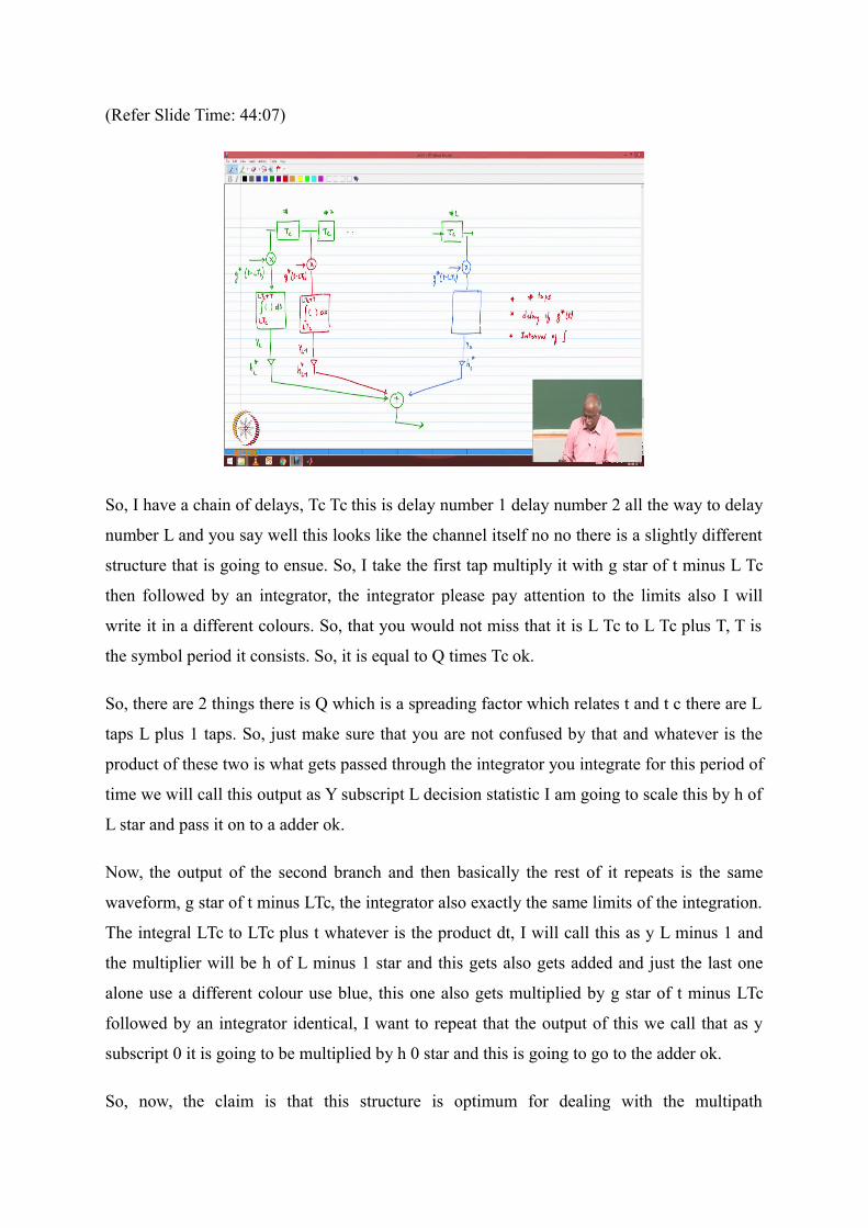
(Refer Slide Time: 44:07)

So, I have a chain of delays, Tc Tc this is delay number 1 delay number 2 all the way to delay

number L and you say well this looks like the channel itself no no there is a slightly different

structure that is going to ensue. So, I take the first tap multiply it with g star of t minus L Tc

then followed by an integrator, the integrator please pay attention to the limits also I will

write it in a different colours. So, that you would not miss that it is L Tc to L Tc plus T, T is

the symbol period it consists. So, it is equal to Q times Tc ok.

So, there are 2 things there is Q which is a spreading factor which relates t and t c there are L

taps L plus 1 taps. So, just make sure that you are not confused by that and whatever is the

product of these two is what gets passed through the integrator you integrate for this period of

time we will call this output as Y subscript L decision statistic I am going to scale this by h of

L star and pass it on to a adder ok.

Now, the output of the second branch and then basically the rest of it repeats is the same

waveform, g star of t minus LTc, the integrator also exactly the same limits of the integration.

The integral LTc to LTc plus t whatever is the product dt, I will call this as y L minus 1 and

the multiplier will be h of L minus 1 star and this gets also gets added and just the last one

alone use a different colour use blue, this one also gets multiplied by g star of t minus LTc

followed by an integrator identical, I want to repeat that the output of this we call that as y

subscript 0 it is going to be multiplied by h 0 star and this is going to go to the adder ok.

So, now, the claim is that this structure is optimum for dealing with the multipath

environment that we have just now described. So, what are the things to keep in mind what I

would like you to pay attention to one is the number of taps that are present it is L plus 1

same as the number of taps of the channel. Second, is the delay of g star the delay that is very

important because when you did g star, we have done something to the there is not just g star

of t. So, delay for of g star of t we have done that and why does that delay play a role and the

third one is the interval of integration. All three things sort of have to come together for us to

build that and again it is very easy.

So, keep referring to that structure and let us write down the first output, the first output is

integral LTc to LTc plus T r of t g star of t minus LTc dt am I correct? And if you go down the

order because the first the reason it was r of t because it was there was no delays, if I go

further down in the delay chain; that means, this dot dot dot dot says along the delay chain

you will get terms of the following LTc to LTc plus t, it will no longer be r of t, but it will be r

of t delayed by some multiple of Tc LTc and, but the rest of the expression is the same g star

of t minus L Tc dt and l is equal to 1 2 all the way to uppercase L. So, basically these are the

outputs that are coming out and these are the ones that have been terminated have been

designated as the decision statistics as y 0 through y l.

So, this particular 1 was designated as y L and. So, basically we look at yL and then quickly

generalized to the other terms.

Student: The gain term.

I am sorry.

Student: The main term edge (Refer Time: 49:35) we had (Refer Time: 49:38) that is after.

Oh no where did where did I mark y of L did I make a mistake no y of L is (Refer Time:

49:40) what ifs.

Student: (Refer Time: 49:47).

Before I do the addition I will bring the gain term. So, the gain term comes after I get the

decision statistic. So, let me just write one term I think in the interest of time let me the, but I

want you to I want you to try writing the rest of it. So, this one this expression can also be

equivalently represented as 0 to T, r of t plus L Tc g star of t dt actually this is a much nicer

form for us to work with because you know intuitively we like to integrate from 0 to t.

So, now write down the expression for this. So, this will be integral 0 to t, the expression for r

of t plus LTc that is h naught u of t plus LTc plus h 1 u of t plus it is u of t minus tc. So, it will

be t plus L minus 1 Tc dot dot dot and the last term will be h subscript L u of t because it

already has u of minus LTc and you are go you are going to take r plus t plus ltc. So, this

whole thing multiplied by g star of t dt.

Now, notice that u of t has got g of t in it. So, g of t g star of t if I integrate I will get h

subscript L and b root Eb did I write down the expression for u of t? I think we did right? No

we have not written the expression for u of t. So, expression for u of t is b times root Eb times

g of t the pulse shape, and g of t is the spread sequence summation Q equal to 0 through Q

minus 1, c of Q the chip waveform gc t minus qTc please you these are the expressions if you

go back. Now, you will get some terms that will be a cross correlation of g of t with some

shifted version of g of t.

So, basically we will get this is of course, the term that we would like to use for making the

decision what of what are the other terms what happens to the noise term? Those are the

things that we need to look at and how is it that a spread spectrum system actually helps us

get what we want and throw away or suppress the things that we do not want; and if you have

already studied rake receivers you will know that this is the structure that actually becomes

the rake receiver.

So, what I would like you to do is if you could try out the expressions that you will get here

when I post it on the on the website, I will also give you the how to write these terms. If you

can write them then we can then pick it up from here and then couple of steps we shall show

how the rake receiver actually if emerges from this analysis. So, we have a chip spaced

equivalent channel which we are trying to use to build an optimal receiver.

Thank you.