Embed Size (px)
Citation preview

Introduction to Unfolding in High Energy Physics
Mikael KuuselaInstitute of Mathematics,
EPFL
Advanced Scientific Computing Workshop,ETH Zurich
July 15, 2014
Mikael Kuusela (EPFL) Unfolding in HEP July 15, 2014 1 / 66

Outline
1 Introduction
2 Basic unfolding methodologyMaximum likelihood estimationRegularized frequentist techniquesBayesian unfolding
3 Challenges in unfoldingChoice of the regularization strengthUncertainty quantificationMC dependence in the smearing matrix
4 Unfolding with RooUnfold
5 Conclusions
Mikael Kuusela (EPFL) Unfolding in HEP July 15, 2014 2 / 66

Outline
1 Introduction
2 Basic unfolding methodologyMaximum likelihood estimationRegularized frequentist techniquesBayesian unfolding
3 Challenges in unfoldingChoice of the regularization strengthUncertainty quantificationMC dependence in the smearing matrix
4 Unfolding with RooUnfold
5 Conclusions
Mikael Kuusela (EPFL) Unfolding in HEP July 15, 2014 3 / 66

The unfolding problem
Unfolding refers to the problem of estimating the particle-leveldistribution of some physical quantity of interest on the basis ofobservations smeared by an imperfect measurement device
What would the distribution look like when measured with a devicehaving a perfect experimental resolution?
Cf. deconvolution in optics, image reconstruction in medical imaging
−5 0 50
500
1000
1500
Physical observable
(b) Smeared intensity
Intensity
Figure : Smeared density
Folding←−−Unfolding−−→
−5 0 50
500
1000
1500
Physical observable
(a) True intensity
Intensity
Figure : True density
Mikael Kuusela (EPFL) Unfolding in HEP July 15, 2014 4 / 66

Why unfold?
Unfolding is usually done to achieve one or more of the following goals:
1 Comparison of the measurement with future theories
2 Comparison of experiments with different responses
3 Input to a subsequent analysis
4 Exploratory data analysis
Unfolding is most often used in measurement analyses (as opposed todiscovery analyses): QCD, electroweak, top, forward physics,...
Mikael Kuusela (EPFL) Unfolding in HEP July 15, 2014 5 / 66

Examples of unfolding in LHC data analysis
Inclusive jet cross section
(GeV)T
Jet p200 300 1000 2000
d|y|
(pb
/GeV
)T
/dp
σ2 d
-510
-110
310
710
1110
1310 )4 10×|y| < 0.5 (
)3 10×0.5 < |y| < 1.0 ( )2 10×1.0 < |y| < 1.5 ( )1 10×1.5 < |y| < 2.0 ( )0 10×2.0 < |y| < 2.5 (
CMS = 7 TeVs
-1L = 5.0 fb R = 0.7Tanti-k
T= p
Fµ=
Rµ
NP Corr.⊗NNPDF2.1
W boson cross section
Hadronic event shape
,Cτln -12 -10 -8 -6 -4 -2
,Cτ
dN/
dln
N1
0.00
0.05
0.10
0.15
0.20
,Cτln -12 -10 -8 -6 -4 -2
,Cτ
dN/
dln
N1
0.00
0.05
0.10
0.15
0.20 > 30 GeV/cT
, R=0.5, pTanti-k< 125 GeV/c
T,190 GeV/c < p
Pythia6Pythia8Herwig++MadGraph+Pythia6Alpgen+Pythia6Data
-1 = 7 TeV, L = 3.2 pbsCMS
Charged particle multiplicity
Mikael Kuusela (EPFL) Unfolding in HEP July 15, 2014 6 / 66

Problem formulation
Notation:
λ ∈ Rp+ bin means of the true histogram
x ∈ Np0 bin counts of the true histogram
µ ∈ Rn+ bin means of the smeared histogram
y ∈ Nn0 bin counts of the smeared histogram
Assume that:1 The true counts are independent and Poisson distributed
x|λ ∼ Poisson(λ), ⊥⊥ xi |λ
2 The propagation of events to neighboring bins is multinomialconditional on xi and independent for each true bin
It follows that the smeared counts are also independent and Poissondistributed
y|λ ∼ Poisson(Kλ), ⊥⊥ yi |λ
Mikael Kuusela (EPFL) Unfolding in HEP July 15, 2014 7 / 66

Problem formulation
Here the elements of the smearing matrix K ∈ Rn×p are given by
Kij = P(smeared event in bin i | true event in bin j)
and assumed to be known
The unfolding problem:
Problem statement
Given the smeared observations y and the Poisson regression model
y|λ ∼ Poisson(Kλ),
what can be said about the means λ of the true histogram?
The problem here is that typically K is an ill-conditioned matrix
Mikael Kuusela (EPFL) Unfolding in HEP July 15, 2014 8 / 66

Unfolding is an ill-posed inverse problem
The unfolding problem is typically ill-posed in the sense that the(pseudo)inverse of K is very sensitive to small perturbations in thedata
From y|λ ∼ Poisson(Kλ) we have that µ = Kλ
We could naıvely estimate λ = K†µ = K†y
But this can lead to catastrophic results!
Mikael Kuusela (EPFL) Unfolding in HEP July 15, 2014 9 / 66

Demonstration of the ill-posedness
−6 −4 −2 0 2 4 60
100
200
300
400
500Smeared histogram
−6 −4 −2 0 2 4 60
100
200
300
400
500True histogram
Mikael Kuusela (EPFL) Unfolding in HEP July 15, 2014 10 / 66

Demonstration of the ill-posedness
−6 −4 −2 0 2 4 6−2.5
−2
−1.5
−1
−0.5
0
0.5
1
1.5
2x 10
13
Pseudoinverse
True
Mikael Kuusela (EPFL) Unfolding in HEP July 15, 2014 11 / 66

Outline
1 Introduction
2 Basic unfolding methodologyMaximum likelihood estimationRegularized frequentist techniquesBayesian unfolding
3 Challenges in unfoldingChoice of the regularization strengthUncertainty quantificationMC dependence in the smearing matrix
4 Unfolding with RooUnfold
5 Conclusions
Mikael Kuusela (EPFL) Unfolding in HEP July 15, 2014 12 / 66

Outline
1 Introduction
2 Basic unfolding methodologyMaximum likelihood estimationRegularized frequentist techniquesBayesian unfolding
3 Challenges in unfoldingChoice of the regularization strengthUncertainty quantificationMC dependence in the smearing matrix
4 Unfolding with RooUnfold
5 Conclusions
Mikael Kuusela (EPFL) Unfolding in HEP July 15, 2014 13 / 66

The likelihood function
The likelihood function in unfolding is:
L(λ) = p(y|λ) =n∏
i=1
p(yi |λ) =n∏
i=1
(∑pj=1 Kijλj
)yiyi !
e−∑p
j=1 Kijλj , λ ∈ Rp+
This function uses our Poisson regression model to link theobservations y with the unknown λ
The likelihood function plays a key role in all sensible unfoldingmethods
In most statistical problems, the maximum of the likelihood, orequivalently the maximum of the log-likelihood, provides a goodestimate of the unknown
In ill-posed problems, this is usually not the case, but the maximumlikelihood solution still provides a good starting point
Mikael Kuusela (EPFL) Unfolding in HEP July 15, 2014 14 / 66

Maximum likelihood estimation
Any histogram that maximizes the log-likelihood of the unfoldingproblem is called a maximum likelihood estimator λMLE of λ
Hence, we want to solve:
maxλ∈Rp
+
log p(y|λ) =n∑
i=1
yi log
p∑j=1
Kijλj
− p∑j=1
Kijλj
+ const
Mikael Kuusela (EPFL) Unfolding in HEP July 15, 2014 15 / 66

Maximum likelihood estimation
Theorem (Vardi et al. (1985))
Assume Kij > 0 and y 6= 0. Then the following hold for the log-likelihoodlog p(y|λ) of the unfolding problem:
1 The log-likelihood has a maximum.
2 The log-likelihood is concave and hence all the maxima are globalmaxima.
3 The maximum is unique if and only if the columns of K are linearlyindependent
So a unique MLE exists when the columns of K are linearlyindependent but how do we find it?
Mikael Kuusela (EPFL) Unfolding in HEP July 15, 2014 16 / 66

Maximum likelihood estimation
Proposition
Let K be an invertible square matrix and assume that λ = K−1y ≥ 0.Then λ is the MLE of λ.
That is, matrix inversion gives us the MLE if K is invertible and theresulting estimate is positive
Note that this result is more restrictive than it may seem
K is often non-squareEven if K was square, it is often not invertibleAnd even if K was invertible, K−1y often contains negative values
Is there a general recipe for finding the MLE?
Mikael Kuusela (EPFL) Unfolding in HEP July 15, 2014 17 / 66

Maximum likelihood estimation
The MLE can always be found computationally by using theexpectation-maximization (EM) algorithm (Dempster et al. (1977))
This is a widely used iterative algorithm for finding maximum likelihoodsolutions in problems that can be seen as containing incompleteobservations
Starting from some initial value λ(0) > 0, the EM iteration forunfolding is given by:
λ(k+1)j =
λ(k)j∑n
i=1 Kij
n∑i=1
Kijyi∑pl=1 Kilλ
(k)l
, j = 1, . . . , p
The convergence of this iteration to an MLE (i.e. λ(k) k→∞−→ λMLE)was proved by Vardi et al. (1985)
Mikael Kuusela (EPFL) Unfolding in HEP July 15, 2014 18 / 66

Maximum likelihood estimation
The EM iteration for finding the MLE in Poisson regression problemshas been rediscovered many times in different fields:
Optics: Richardson (1972)Astronomy: Lucy (1974)Tomography: Shepp and Vardi (1982); Lange and Carson (1984); Vardiet al. (1985)HEP: Kondor (1983); Multhei and Schorr (1987); Multhei et al. (1987,1989); D’Agostini (1995)
In modern use, the algorithm is most often called D’Agostini iterationin HEP and Lucy–Richardson deconvolution in astronomy and optics
In HEP, also the name “Bayesian unfolding” is used but this is anunfortunate misnomer
D’Agostini iteration is a fully frequentist technique for finding the MLEThere is nothing Bayesian about it!
Mikael Kuusela (EPFL) Unfolding in HEP July 15, 2014 19 / 66

D’Agostini demo, k = 0
−10 −5 0 5 100
100
200
300
400
500µy
Kλ(k)
Figure : Smeared histogram
−10 −5 0 5 100
100
200
300
400
500
λλ(k)
Figure : True histogram
Mikael Kuusela (EPFL) Unfolding in HEP July 15, 2014 20 / 66

D’Agostini demo, k = 100
−10 −5 0 5 100
100
200
300
400
500µy
Kλ(k)
Figure : Smeared histogram
−10 −5 0 5 100
100
200
300
400
500
λλ(k)
Figure : True histogram
Mikael Kuusela (EPFL) Unfolding in HEP July 15, 2014 21 / 66

D’Agostini demo, k = 10000
−10 −5 0 5 100
100
200
300
400
500µy
Kλ(k)
Figure : Smeared histogram
−10 −5 0 5 100
200
400
600
800
λλ(k)
Figure : True histogram
Mikael Kuusela (EPFL) Unfolding in HEP July 15, 2014 22 / 66
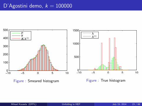
D’Agostini demo, k = 100000
−10 −5 0 5 100
100
200
300
400
500µy
Kλ(k)
Figure : Smeared histogram
−10 −5 0 5 100
500
1000
1500
λλ(k)
Figure : True histogram
Mikael Kuusela (EPFL) Unfolding in HEP July 15, 2014 23 / 66

Outline
1 Introduction
2 Basic unfolding methodologyMaximum likelihood estimationRegularized frequentist techniquesBayesian unfolding
3 Challenges in unfoldingChoice of the regularization strengthUncertainty quantificationMC dependence in the smearing matrix
4 Unfolding with RooUnfold
5 Conclusions
Mikael Kuusela (EPFL) Unfolding in HEP July 15, 2014 24 / 66

Regularization by early stopping of the EM iteration
We have seen that unfortunately the MLE itself is often useless
Due to the ill-posedness of the problem, it exhibits large, unphysicalfluctuationsIn other words, the likelihood function alone does not contain enoughinformation to constrain the solution
As the EM iteration proceeds, the solutions will typically first improvebut will start to degrade at some point
This is because the algorithm will start overfitting to the Poissonfluctuations in y
This behavior can be exploited by stopping the iteration beforeunphysical features start to appear
The number of iterations k now becomes a regularization parameterthat controls the trade-off between fitting the data and tamingunphysical features
Mikael Kuusela (EPFL) Unfolding in HEP July 15, 2014 25 / 66

D’Agostini demo, k = 100
−10 −5 0 5 100
100
200
300
400
500µy
Kλ(k)
Figure : Smeared histogram
−10 −5 0 5 100
100
200
300
400
500
λλ(k)
Figure : True histogram
Mikael Kuusela (EPFL) Unfolding in HEP July 15, 2014 26 / 66

Penalized maximum likelihood estimation
Early stopping of the EM iteration seems a bit ad-hoc
Is there a more principled way of finding good solutions?
Ideally we would like to find a solution that fits the data but at thesame time seems physically plausible
Let’s consider a penalized maximum likelihood problem:
maxλ∈Rp
+
F (λ) = log p(y|λ)− δP(λ),
Here:
P(λ) is a penalty function which obtains large values for physicallyimplausible solutionsδ > 0 is a regularization parameter which controls the balance betweenmaximizing the likelihood and minimizing the penalty
Typically P(λ) is a measure of the curvature of the solution
I.e., it penalizes for large oscillations
Mikael Kuusela (EPFL) Unfolding in HEP July 15, 2014 27 / 66

From penalized likelihood to Tikhonov regularization
To simplify this optimization problem, we use a Gaussianapproximation of the Poisson likelihood
y|λ ∼ Poisson(Kλ) ≈ N(Kλ, C),
where C = diag(y)
Hence the objective function becomes:
F (λ) = log p(y|λ)− δP(λ)
=n∑
i=1
yi log
p∑j=1
Kijλj
− p∑j=1
Kijλj
− δP(λ) + const
≈ −1
2(y −Kλ)TC−1(y −Kλ)− δP(λ) + const
Mikael Kuusela (EPFL) Unfolding in HEP July 15, 2014 28 / 66

From penalized likelihood to Tikhonov regularization
We furthermore drop the positivity constraint and absorb the factor1/2 into the penalty to obtain
λ = arg maxλ∈Rp
−(y −Kλ)TC−1(y −Kλ)− δP(λ)
= arg minλ∈Rp
(y −Kλ)TC−1(y −Kλ) + δP(λ)
We see that we have ended up with a penalized χ2 problem
This is typically called (generalized) Tikhonov regularization
Mikael Kuusela (EPFL) Unfolding in HEP July 15, 2014 29 / 66

How to choose the penalty?
The penalty term should reflect the analyst’s a priori understanding ofthe desired solution
Common choices include:
Norm of the solution: P(λ) = ‖λ‖2Curvature of the solution: P(λ) = ‖Lλ‖2, where L is a discretized 2ndderivative operator“SVD” unfolding (Hocker and Kartvelishvili, 1996):
P(λ) =
∥∥∥∥∥∥∥∥∥L
λ1/λ
MC1
λ2/λMC2
...λp/λ
MCp
∥∥∥∥∥∥∥∥∥2
,
where λMC is a MC prediction for λTUnfold1 (Schmitt, 2012): P(λ) = ‖L(λ− λMC)‖2
1Also more general penalty terms are allowed in TUnfoldMikael Kuusela (EPFL) Unfolding in HEP July 15, 2014 30 / 66

Least squares estimation with the pseudoinverse
Consider the least squares problem
minx∈Rp‖Ax− y‖2,
where A ∈ Rn×p, x ∈ Rp and y ∈ Rn
This problem always has a solution, but it may not be unique
A solution is always given by the Moore–Penrose pseudoinverse of A:
xLS = A†y
When there are multiple solutions, the pseudoinverse gives the onewith the smallest norm
When A has full column rank, the solution is unique
In this special case, the pseudoinverse is given by A† = (ATA)−1AT
Hence, the least squares solution is: xLS = (ATA)−1ATy
Mikael Kuusela (EPFL) Unfolding in HEP July 15, 2014 31 / 66

Finding the Tikhonov regularized solution
We will now find an explicit form of the Tikhonov regularized estimator
λ = arg minλ∈Rp
(y −Kλ)TC−1(y −Kλ) + δ‖Lλ‖2
by rewriting this as a least squares problemThis approach also easily generalizes to penalty terms involving λMC
Let us rewrite:
C−1
= diag
(1
y1, . . . ,
1
yn
)= diag
(1√
y1, . . . ,
1√
yn
)︸ ︷︷ ︸
:=A
diag
(1√
y1, . . . ,
1√
yn
)︸ ︷︷ ︸
:=A
= AA = ATA
Defining y := Ay and K := AK, our optimization problem becomes
λ = arg minλ∈Rp
(y − Kλ)T(y − Kλ) + δ‖Lλ‖2
Mikael Kuusela (EPFL) Unfolding in HEP July 15, 2014 32 / 66

Finding the Tikhonov regularized solution
We can rewrite the objective function as follows:
(y − Kλ)T(y − Kλ) + δ‖Lλ‖2
= ‖Kλ− y‖2 + ‖√δLλ‖2
=
∥∥∥∥[Kλ− y√δLλ
]∥∥∥∥2=
∥∥∥∥[ K√δL
]λ−
[y0
]∥∥∥∥2Here we recognize a least squares problem, so a minimizer is given by
λ =
[K√δL
]† [y0
]
Mikael Kuusela (EPFL) Unfolding in HEP July 15, 2014 33 / 66

Finding the Tikhonov regularized solution
Assuming that ker(K) ∩ ker(L) = {0}, the minimizer is unique andcan be simplified as follows:
λ =
[K√δL
]† [y0
]
=
([K√δL
]T [K√δL
])−1 [K√δL
]T [y0
]
=
([K
T √δLT
] [ K√δL
])−1 [K
T √δLT
] [y0
]=(
KT
K + δLTL)−1
KT
y
=(
KTC−1
K + δLTL)−1
KTC−1
y
Hence we have obtained an explicit, closed-form solution for theTikhonov regularization problem
Mikael Kuusela (EPFL) Unfolding in HEP July 15, 2014 34 / 66

Demonstration of Tikhonov regularization, P(λ) = ‖λ‖2
−6 −4 −2 0 2 4 6−100
0
100
200
300
400
500
600
Tikhonov regularization
True
Mikael Kuusela (EPFL) Unfolding in HEP July 15, 2014 35 / 66

Outline
1 Introduction
2 Basic unfolding methodologyMaximum likelihood estimationRegularized frequentist techniquesBayesian unfolding
3 Challenges in unfoldingChoice of the regularization strengthUncertainty quantificationMC dependence in the smearing matrix
4 Unfolding with RooUnfold
5 Conclusions
Mikael Kuusela (EPFL) Unfolding in HEP July 15, 2014 36 / 66

Bayesian unfolding
In Bayesian unfolding, the inferences about λ are based on theposterior distribution p(λ|y)
This is obtained using Bayes’ rule:
p(λ|y) =p(y|λ)p(λ)
p(y)=
p(y|λ)p(λ)∫Rp+
p(y|λ′)p(λ′) dλ′, λ ∈ Rp
+
where the likelihood p(y|λ) is the same as earlier and p(λ) is a priordistribution for λThe most common choices as a point estimator of λ are:
The posterior mean: λ = E[λ|y] =∫Rp
+λp(λ|y) dλ
The maximum a posteriori (MAP) estimator: λ = arg maxλ∈Rp
+
p(λ|y)
The width of the posterior distribution p(λ|y) can be used to quantifyuncertainty regarding λ
But note that the interpretation of the resulting Bayesian credibleintervals is different from frequentist confidence intervals
Mikael Kuusela (EPFL) Unfolding in HEP July 15, 2014 37 / 66

Regularization using the prior
In the Bayesian approach, the prior density p(λ) regularizes theotherwise ill-posed problem
It concentrates the probability mass of the posterior on physicallyplausible solutions
The prior is typically of the form
p(λ) ∝ exp (−δP(λ)) , λ ∈ Rp+,
where P(λ) is a function characterizing a priori plausible solutions andδ > 0 is a hyperparameter controlling the scale of the prior density
For example, choosing P(λ) = ‖Lλ‖2, where L a discretized 2ndderivative operator, leads to the positivity-constrained Gaussiansmoothness prior
p(λ) ∝ exp(−δ‖Lλ‖2
), λ ∈ Rp
+
Mikael Kuusela (EPFL) Unfolding in HEP July 15, 2014 38 / 66

Connection between Bayesian unfolding and penalized MLE
Notice that when p(λ) ∝ exp (−δP(λ)), the Bayesian MAP solutioncoincides with the penalized maximum likelihood estimator:
λMAP = arg maxλ∈Rp
+
p(λ|y)
= arg maxλ∈Rp
+
log p(λ|y)
= arg maxλ∈Rp
+
log p(y|λ) + log p(λ)
= arg maxλ∈Rp
+
log p(y|λ)− δP(λ)
= λPMLE
So the penalty term δP(λ) can either be interpreted as a Bayesianprior or as a frequentist regularization term
The Bayesian interpretation has the advantage that we can visualizethe prior p(λ) by, e.g., drawing samples from it
Mikael Kuusela (EPFL) Unfolding in HEP July 15, 2014 39 / 66

A note about Bayesian computations
To be able to compute the posterior mean E[λ|y] or form the Bayesiancredible intervals, we need to be able to evaluate the posterior
p(λ|y) =p(y|λ)p(λ)∫
Rp+
p(y|λ′)p(λ′) dλ′
But the denominator is an intractable high-dimensional integral...Luckily, it turns out that it is possible to sample from the posteriorwithout evaluating the denominator
The sample mean and sample quantiles can then be used to computethe posterior mean and the credible intervals
The class of algorithms that enable this are called Markov chainMonte Carlo (MCMC) samplers and are based on a Markov chainwhose equilibrium distribution is the posterior p(λ|y)
The single-component Metropolis–Hastings sampler of Saquib et al.(1998) is particularly well-suited for the unfolding problem and seemsto also work well in practice
Mikael Kuusela (EPFL) Unfolding in HEP July 15, 2014 40 / 66

Outline
1 Introduction
2 Basic unfolding methodologyMaximum likelihood estimationRegularized frequentist techniquesBayesian unfolding
3 Challenges in unfoldingChoice of the regularization strengthUncertainty quantificationMC dependence in the smearing matrix
4 Unfolding with RooUnfold
5 Conclusions
Mikael Kuusela (EPFL) Unfolding in HEP July 15, 2014 41 / 66

Outline
1 Introduction
2 Basic unfolding methodologyMaximum likelihood estimationRegularized frequentist techniquesBayesian unfolding
3 Challenges in unfoldingChoice of the regularization strengthUncertainty quantificationMC dependence in the smearing matrix
4 Unfolding with RooUnfold
5 Conclusions
Mikael Kuusela (EPFL) Unfolding in HEP July 15, 2014 42 / 66

Choice of the regularization strength
All unfolding methods involve a free parameter controlling thestrength of the regularization
The parameter δ in Tikhonov regularization and Bayesian unfolding,the number of iterations in D’Agostini
This parameter is typically difficult to choose using only a prioriinformation
But its value usually has a major impact on the unfolded spectrum
Most LHC analyses choose the regularization parameter using MCstudies
But this may create an undesired MC bias
It would be better to choose the regularization parameter based onthe observed data y
Mikael Kuusela (EPFL) Unfolding in HEP July 15, 2014 43 / 66

Data-dependent choice of the regularization strength
Many methods for using the observed data y to choose theregularization strength have been proposed in the literature:
Goodness-of-fit test in the smeared space (Veklerov and Llacer, 1987)Empirical Bayes estimation (Kuusela and Panaretos, 2014)L-curve (Hansen, 1992)(Generalized) cross validation (Wahba, 1990)...
At the moment, we have very limited experience about the relativemerits of these methods in HEP unfolding
Mikael Kuusela (EPFL) Unfolding in HEP July 15, 2014 44 / 66

Goodness-of-fit for choosing the regularization strength
We present here a simplified version of the procedure proposed byVeklerov and Llacer (1987)
Let µ = Kλ be the estimated smeared mean
Consider the χ2 statistic
T = (µ− y)TC−1(µ− y),
where C = diag(µ)
If y ∼ Poisson(µ), then asymptotically Ta∼ χ2
n, where n is thenumber of bins in y
Hence, E[T ] ≈ n
This suggests that we should choose the regularization strength sothat T is as close as possible to n
Note that this provides a balance between overfitting (T < n) andunderfitting (T > n) the data
Mikael Kuusela (EPFL) Unfolding in HEP July 15, 2014 45 / 66

Outline
1 Introduction
2 Basic unfolding methodologyMaximum likelihood estimationRegularized frequentist techniquesBayesian unfolding
3 Challenges in unfoldingChoice of the regularization strengthUncertainty quantificationMC dependence in the smearing matrix
4 Unfolding with RooUnfold
5 Conclusions
Mikael Kuusela (EPFL) Unfolding in HEP July 15, 2014 46 / 66

Uncertainty quantification
Proper uncertainty quantification is one of the main challenges inunfolding
By uncertainty quantification, we mean computing bin-wisefrequentist confidence intervals at 1− α confidence level:
infλ∈Rp
+
Pλ[λi ,L(y) ≤ λi ≤ λi ,U(y)] = 1− α
In practice, we can only hope to satisfy this approximately for finitesample sizes
Mikael Kuusela (EPFL) Unfolding in HEP July 15, 2014 47 / 66

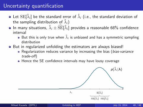
Uncertainty quantification
Let SE[λi ] be the standard error of λi (i.e., the standard deviation ofthe sampling distribution of λi )
In many situations, λi ± SE[λi ] provides a reasonable 68% confidenceinterval
But this is only true when λi is unbiased and has a symmetric samplingdistribution
But in regularized unfolding the estimators are always biased!Regularization reduces variance by increasing the bias (bias-variancetrade-off)Hence the SE confidence intervals may have lousy coverage
SE[λi ] SE[λi ]
p(λi |λ)
λi = E[λi ]
Mikael Kuusela (EPFL) Unfolding in HEP July 15, 2014 48 / 66
Uncertainty quantification
Let SE[λi ] be the standard error of λi (i.e., the standard deviation ofthe sampling distribution of λi )
In many situations, λi ± SE[λi ] provides a reasonable 68% confidenceinterval
But this is only true when λi is unbiased and has a symmetric samplingdistribution
But in regularized unfolding the estimators are always biased!Regularization reduces variance by increasing the bias (bias-variancetrade-off)Hence the SE confidence intervals may have lousy coverage
SE[λi ] SE[λi ]
p(λi |λ)
λi E[λi ]
Mikael Kuusela (EPFL) Unfolding in HEP July 15, 2014 48 / 66

Demonstration with Tikhonov regularization, P(λ) = ‖λ‖2
−5 0 5−2000
−1000
0
1000
2000
δ = 1e−05
λ
λ± SE[λ]
−5 0 5−100
0
100
200
300
400
500
600
δ = 0.001
λ
λ± SE[λ]
−5 0 5−100
0
100
200
300
400
500
600
δ = 0.01
λ
λ± SE[λ]
−5 0 5−100
0
100
200
300
400
500
600
δ = 1
λ
λ± SE[λ]
Mikael Kuusela (EPFL) Unfolding in HEP July 15, 2014 49 / 66

Uncertainty quantification
The uncertainties returned by RooUnfold are estimates of thestandard errors computed either using error propagation or resampling
Hence these uncertainties should be understood as estimates of thespread of the sampling distribution of λThese should only be understood as approximate confidence intervals ifit can be shown that the bias is negligible
Bootstrap resampling provides an attractive way of formingapproximate confidence intervals that take into account the bias andthe potential skewness of p(λi |λ) (Kuusela and Panaretos, 2014)
Mikael Kuusela (EPFL) Unfolding in HEP July 15, 2014 50 / 66

Outline
1 Introduction
2 Basic unfolding methodologyMaximum likelihood estimationRegularized frequentist techniquesBayesian unfolding
3 Challenges in unfoldingChoice of the regularization strengthUncertainty quantificationMC dependence in the smearing matrix
4 Unfolding with RooUnfold
5 Conclusions
Mikael Kuusela (EPFL) Unfolding in HEP July 15, 2014 51 / 66

MC dependence in the smearing matrix
The smearing matrix K is typically estimated using Monte Carlo
In addition to a statistical error due to the finite sample size, there aretwo sources of systematics in K:
1 The matrix depends on the shape of the spectrum within each true bin
Kij =
∫Fi
∫Ej
k(y , x)f (x) dx dy∫Ej
f (x) dx, i = 1, . . . , n, j = 1, . . . , p
2 The smearing of the variable of interest may depend on the MCdistribution of some auxiliary variables
For example, the energy resolution of jets depends on thepseudorapidity distribution of the jets
The first problem can be alleviated by making the true bins smaller atthe cost of increased ill-posedness of the problem
Mikael Kuusela (EPFL) Unfolding in HEP July 15, 2014 52 / 66

Outline
1 Introduction
2 Basic unfolding methodologyMaximum likelihood estimationRegularized frequentist techniquesBayesian unfolding
3 Challenges in unfoldingChoice of the regularization strengthUncertainty quantificationMC dependence in the smearing matrix
4 Unfolding with RooUnfold
5 Conclusions
Mikael Kuusela (EPFL) Unfolding in HEP July 15, 2014 53 / 66

Introduction to RooUnfold
RooUnfold (Adye, 2011) an unfolding framework for ROOT thatprovides an interface for many standard unfolding methods
Written by Tim Adye, Richard Claridge, Kerstin Tackmann andFergus Wilson
RooUnfold is currently the most commonly used unfolding frameworkamong the LHC experiments although other implementations are alsooccasionally usedRooUnfold includes the following unfolding techniques:
1 Matrix inversion2 D’Agostini iteration3 The SVD flavor of Tikhonov regularization4 The TUnfold flavor of Tikhonov regularization
There is also an implementation for the so-called bin-by-bin unfoldingtechnique
This is an obsolete method that replaces the full response matrix K bya diagonal approximation and while doing so introduces a huge MC biasThis method should not be used!
Mikael Kuusela (EPFL) Unfolding in HEP July 15, 2014 54 / 66

RooUnfold classes
Figure from Adye (2011)
Mikael Kuusela (EPFL) Unfolding in HEP July 15, 2014 55 / 66

RooUnfoldInvert
RooUnfoldInvert(const RooUnfoldResponse* res, const TH1*
meas, const char* name = 0, const char* title = 0)
This is the most basic method: it estimates λ using λ = K−1y
Remember that when λ is positive, this is the MLE
res contains the response matrix K
meas contains the smeared data y
The standard error of λ is estimated using standard error propagation
Mikael Kuusela (EPFL) Unfolding in HEP July 15, 2014 56 / 66

RooUnfoldBayes
RooUnfoldBayes(const RooUnfoldResponse* res, const TH1*
meas, Int t niter = 4, Bool t smoothit = false, const char*
name = 0, const char* title = 0)
This implements the D’Agostini/Lucy-Richardson/EM iteration forfinding the MLERemember that despite the name this is not a Bayesian techniqueThe iteration is started from the MC spectrum, i.e., λ(0) = λMC
contained in resniter is the number of iterations
For small niter, the solution is biased towards λMC; for large niter,we get a solution close to the MLENote that the default niter = 4 is completely arbitrary and with nooptimality guarantees
smoothit can be used to enable a smoothed version of the EMiteration (outside the scope of this course)By default, the standard error of λ is estimated using errorpropagation at each iteration of the algorithm
Mikael Kuusela (EPFL) Unfolding in HEP July 15, 2014 57 / 66

RooUnfoldSvd
RooUnfoldSvd(const RooUnfoldResponse* res, const TH1* meas,
Int t kreg = 0, Int t ntoyssvd = 1000, const char* name = 0,
const char* title = 0)
This implements the SVD flavor of Tikhonov regularization, i.e.,
λ = arg minλ∈Rp
(y −Kλ)TC−1(y −Kλ) + δ
∥∥∥∥∥∥∥∥∥L
λ1/λ
MC1
λ2/λMC2
...λp/λ
MCp
∥∥∥∥∥∥∥∥∥2
,
where λMC is again contained in res
This is a wrapper for the TSVDUnfold class by K. Tackmannkreg chooses the number of significant singular values in a certaintransformation of the smearing matrix K
Small kreg corresponds to a large δ and a large kreg to a small δ
The standard error of λ is estimated by resampling ntoyssvdobservations
Also includes a contribution from the uncertainty of KMikael Kuusela (EPFL) Unfolding in HEP July 15, 2014 58 / 66

RooUnfoldTUnfold
RooUnfoldTUnfold(const RooUnfoldResponse* res, const TH1*
meas, TUnfold::ERegMode reg = TUnfold::kRegModeDerivative,
const char* name = 0, const char* title = 0)
This implements the TUnfold flavor of Tikhonov regularization, i.e.,
λ = arg minλ∈Rp
(y −Kλ)TC−1(y −Kλ) + δ‖L(λ− λMC)‖2,
where the minimizer is found subject to an additional area constraint2
This is a wrapper for the TUnfold class by S. SchmittTUnfold actually provides a lot of extra functionality which cannot beaccessed through RooUnfold
The form of the matrix L is chosen using regThe supported choices are identity, 1st derivative and 2nd derivative
The regularization parameter δ is chosen using theSetRegParm(Double t parm) method
If δ is not chosen manually, it is found automatically using the L-curvetechnique, but this only seems to work when n� p
2In the case of the TUnfold wrapper, the RooUnfold documentation is not explicitabout the choice of λMC (it does not seem to come from res in this case)
Mikael Kuusela (EPFL) Unfolding in HEP July 15, 2014 59 / 66

RooUnfold practical
Start by downloading the code template at:
www.cern.ch/mkuusela/ETH_workshop_July_2014/
RooUnfoldExercise.cxx
A set of exercises based on this code can be found at:www.cern.ch/mkuusela/ETH_workshop_July_2014/
practical.pdf
Useful supplementary materialThese slides:
www.cern.ch/mkuusela/ETH_workshop_July_2014/
slides.pdf
RooUnfold website:
http://hepunx.rl.ac.uk/~adye/software/unfold/
RooUnfold.html
RooUnfold class documentation:
http://hepunx.rl.ac.uk/~adye/software/unfold/
htmldoc/RooUnfold.html
Mikael Kuusela (EPFL) Unfolding in HEP July 15, 2014 60 / 66

Outline
1 Introduction
2 Basic unfolding methodologyMaximum likelihood estimationRegularized frequentist techniquesBayesian unfolding
3 Challenges in unfoldingChoice of the regularization strengthUncertainty quantificationMC dependence in the smearing matrix
4 Unfolding with RooUnfold
5 Conclusions
Mikael Kuusela (EPFL) Unfolding in HEP July 15, 2014 61 / 66

Conclusions
Unfolding is a complex data analysis task that involves severalassumptions and approximations
It is crucial to understand the ingredients that go into an unfoldingprocedureUnfolding algorithms should never be used as black boxes!
All unfolding methods are based on complementing the likelihood byadditional information about physically plausible solutionsThe most popular techniques are the D’Agostini iteration and variousflavors of Tikhonov regularizationBeware when using RooUnfold that:
There is a MC dependence in both the smearing matrix and theregularizationThe uncertainties should be understood as standard errors and do notnecessarily provide good coverage propertiesThe regularization parameter has a major impact on the solution andshould be chosen in a data-dependent way
There is plenty room for further improvements in both unfoldingmethodology and software
Mikael Kuusela (EPFL) Unfolding in HEP July 15, 2014 62 / 66

References I
T. Adye. Unfolding algorithms and tests using RooUnfold. In H. B. Prosper andL. Lyons, editors, Proceedings of the PHYSTAT 2011 Workshop on StatisticalIssues Related to Discovery Claims in Search Experiments and Unfolding,CERN-2011-006, pages 313–318, CERN, Geneva, Switzerland, 17–20 January2011.
G. D’Agostini. A multidimensional unfolding method based on Bayes’ theorem.Nuclear Instruments and Methods A, 362:487–498, 1995.
A. P. Dempster, N. M. Laird, and D. B. Rubin. Maximum likelihood fromincomplete data via the EM algorithm. Journal of the Royal Statistical Society.Series B (Methodological), 39(1):1–38, 1977.
P. C. Hansen. Analysis of discrete ill-posed problems by means of the L-curve.SIAM Review, 34(4):561–580, 1992.
A. Hocker and V. Kartvelishvili. SVD approach to data unfolding. NuclearInstruments and Methods in Physics Research A, 372:469–481, 1996.
Mikael Kuusela (EPFL) Unfolding in HEP July 15, 2014 63 / 66

References II
A. Kondor. Method of convergent weights – An iterative procedure for solvingFredholm’s integral equations of the first kind. Nuclear Instruments andMethods, 216:177–181, 1983.
M. Kuusela and V. M. Panaretos. Empirical Bayes unfolding of elementaryparticle spectra at the Large Hadron Collider. arXiv:1401.8274 [stat.AP], 2014.
K. Lange and R. Carson. EM reconstruction algorithms for emission andtransmission tomography. Journal of Computer Assisted Tomography, 8(2):306–316, 1984.
L. B. Lucy. An iterative technique for the rectification of observed distributions.Astronomical Journal, 79(6):745–754, 1974.
H. N. Multhei and B. Schorr. On an iterative method for the unfolding of spectra.Nuclear Instruments and Methods in Physics Research A, 257:371–377, 1987.
H. N. Multhei, B. Schorr, and W. Tornig. On an iterative method for a class ofintegral equations of the first kind. Mathematical Methods in the AppliedSciences, 9:137–168, 1987.
Mikael Kuusela (EPFL) Unfolding in HEP July 15, 2014 64 / 66

References III
H. N. Multhei, B. Schorr, and W. Tornig. On properties of the iterativemaximum likelihood reconstruction method. Mathematical Methods in theApplied Sciences, 11:331–342, 1989.
W. H. Richardson. Bayesian-based iterative method of image restoration. Journalof the Optical Society of America, 62(1):55–59, 1972.
S. S. Saquib, C. A. Bouman, and K. Sauer. ML parameter estimation for Markovrandom fields with applications to Bayesian tomography. IEEE Transactions onImage Processing, 7(7):1029–1044, 1998.
S. Schmitt. TUnfold, an algorithm for correcting migration effects in high energyphysics. Journal of Instrumentation, 7:T10003, 2012.
L. A. Shepp and Y. Vardi. Maximum likelihood reconstruction for emissiontomography. IEEE Transactions on Medical Imaging, 1(2):113–122, 1982.
Y. Vardi, L. Shepp, and L. Kaufman. A statistical model for positron emissiontomography. Journal of the American Statistical Association, 80(389):8–20,1985.
Mikael Kuusela (EPFL) Unfolding in HEP July 15, 2014 65 / 66

References IV
E. Veklerov and J. Llacer. Stopping rule for the MLE algorithm based onstatistical hypothesis testing. IEEE Transactions on Medical Imaging, 6(4):313–319, 1987.
G. Wahba. Spline Models for Observational Data. SIAM, 1990.
Mikael Kuusela (EPFL) Unfolding in HEP July 15, 2014 66 / 66

Backup
Mikael Kuusela (EPFL) Unfolding in HEP July 15, 2014 67 / 66

Uncertainty quantification with the bootstrap
The bootstrap sample can be obtained as follows:1 Unfold y to obtain λ2 Fold λ to obtain µ = Kλ3 Obtain a resampled observation y∗ ∼ Poisson(µ)4 Unfold y∗ to obtain λ∗
5 Repeat R times from 3
The bootstrap sample {λ∗(r)}Rr=1 follows the sampling distribution of
λ if the true value of λ was the observed value of our estimator
I.e., it is our best understanding of the sampling distribution of λ forthe data at hand
This procedure also enables us to take into account thedata-dependent choice of the regularization strength
This is very difficult to do using competing methods
Mikael Kuusela (EPFL) Unfolding in HEP July 15, 2014 68 / 66

Uncertainty quantification with the bootstrap
The bootstrap sample can be used to compute 1− α basic bootstrapintervals to serve as approximate 1− α confidence intervals for λi :
[λi ,L, λi ,U ] = [2λi − λ∗i ,1−α/2, 2λi − λ∗i ,α/2],
where λ∗i ,α denotes the α-quantile of the bootstrap sample {λ∗(r)i }Rr=1
This can be understood as the bootstrap analogue of the Neymanconstruction of confidence intervals
α/2 α/2
p(θ|θ = θ0)
p(θ|θ = θU)p(θ|θ = θL)
θL θ0 θU
Mikael Kuusela (EPFL) Unfolding in HEP July 15, 2014 69 / 66

Uncertainty quantification with the bootstrap
The bootstrap sample can be used to compute 1− α basic bootstrapintervals to serve as approximate 1− α confidence intervals for λi :
[λi ,L, λi ,U ] = [2λi − λ∗i ,1−α/2, 2λi − λ∗i ,α/2],
where λ∗i ,α denotes the α-quantile of the bootstrap sample {λ∗(r)i }Rr=1
This can be understood as the bootstrap analogue of the Neymanconstruction of confidence intervals
α/2 α/2
p(θ|θ = θ0) = g(θ)
g(θ + θ0 − θU)g(θ + θ0 − θL)
θL θ0 θU
Mikael Kuusela (EPFL) Unfolding in HEP July 15, 2014 69 / 66
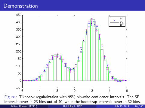
Demonstration
−6 −4 −2 0 2 4 6−50
0
50
100
150
200
250
300
350
400
450
λ
λSEBS
Figure : Tikhonov regularization with 95% bin-wise confidence intervals. The SEintervals cover in 23 bins out of 40, while the bootstrap intervals cover in 32 bins.
Mikael Kuusela (EPFL) Unfolding in HEP July 15, 2014 70 / 66