PHYSICAL REVIEW E 86, 046302 (2012)

Fractal space-scale unfolding mechanism for energy-efficient turbulent mixing

S. Laizet* and J. C. Vassilicos†

Turbulence, Mixing and Flow Control Group, Department of Aeronautics, South Kensington, Imperial College,London SW7 2BZ, United Kingdom‡

(Received 1 May 2012; published 1 October 2012)

Using top-end high fidelity computer simulations we demonstrate the existence of a mechanism present inturbulent flows generated by multiscale or fractal objects and which has its origin in the multiscale or fractalspace-scale structure of such turbulent flow generators. As a result of this space-scale unfolding mechanism,fractal grids can enhance scalar transfer and turbulent diffusion by one order of magnitude while at the same timereduce pressure drop by half. This mechanism must be playing a decisive role in environmental, atmospheric,ocean, and river transport processes wherever turbulence originates from multiscale or fractal objects such astrees, forests, mountains, rocky riverbeds, and coral reefs. It also ushers in the concept of fractal design ofturbulence which may hold the power of setting entirely new mixing and cooling industrial standards.

DOI: 10.1103/PhysRevE.86.046302 PACS number(s): 47.27.wj, 47.27.E−

Nature is replete with multiscale or fractal objects, suchas trees, forests, mountains, coral reefs, rough ocean surfaces,and irregular sea and riverbeds which interact with air or waterflow and create turbulence. The question arises whether theturbulent flows thus generated can transport and mix heat,moisture, biological, chemical and/or polluting substances andperhaps also propagate fires faster and/or more efficiently thanturbulent flows conventionally studied in the laboratory.

This fundamental question has also direct applied physicsimplications. Static obstacles of various shapes, called mixingelements by the industries involved, are routinely placed insideindustrial static inline mixers or exhaust ducts in order toreorient the flow in various alternate directions and/or createturbulence so as to achieve mixing [1]. The nuclear and processindustries routinely use so-called spacer grids and rod bafflesto achieve enhanced heat transfer and cooling in cylindricalgeometries such as shell-and-tube heat exchangers [2]. Is therean advantage in copying nature and designing fractal spacergrids and baffles as well as fractal mixing elements for staticinline mixers?

Fractal geometry has been a mathematical and, in science,a mostly descriptive activity [3,4] till the late 1980s and 1990swhen research on the linear physics of fractals started [5,6].Studies of turbulent flows with fractal or multiscale inletboundary conditions have only recently been emerging [7–10].In this paper we report on the stirring and transport propertiesof turbulent flows generated by fractal objects.

A good setting for such a study is grid-generated turbulentflow [11–13] in a wind tunnel or water channel. In such asetting, the grid is placed at and covers the entry of a tunnelor channel test section and the flow moves through the gridtowards the test section and along it. As the flow moves throughthe grid it becomes turbulent. This turbulence determines boththe pressure drop across the grid and the random stirring whichcan cause transfers, turbulent diffusion and, thereby, mixing.

In this computational study we calculate and comparethe effects of fractal and regular grids on scalar transfer

*s.laizet@imperial.ac.uk†j.c.vassilicos@imperial.ac.uk‡www.imperial.ac.uk/tmfc

and turbulent diffusion efficiencies [14–16]. As a result wereport a mechanism which greatly increases scalar transfer andturbulent diffusion and at the same time reduces pressure dropand therefore power losses. We carry out this study in a genericconfiguration which can just about be reached by currenttop-end high performance computing and massive numericalcode parallelization. It is possible, of course, to study morespecific configurations in the laboratory, but it is extremelyhard, if not impossible, to obtain full flow and pressure fieldinformation from laboratory measurements in the way that ournumerical computations allow us to do. These entire flow andpressure fields provide a wealth of information which enablesus to draw simple conclusions and understanding such as thespace-scale unfolding (SSU) mechanism which has potentialfor broad applicability in the natural and applied sciences.

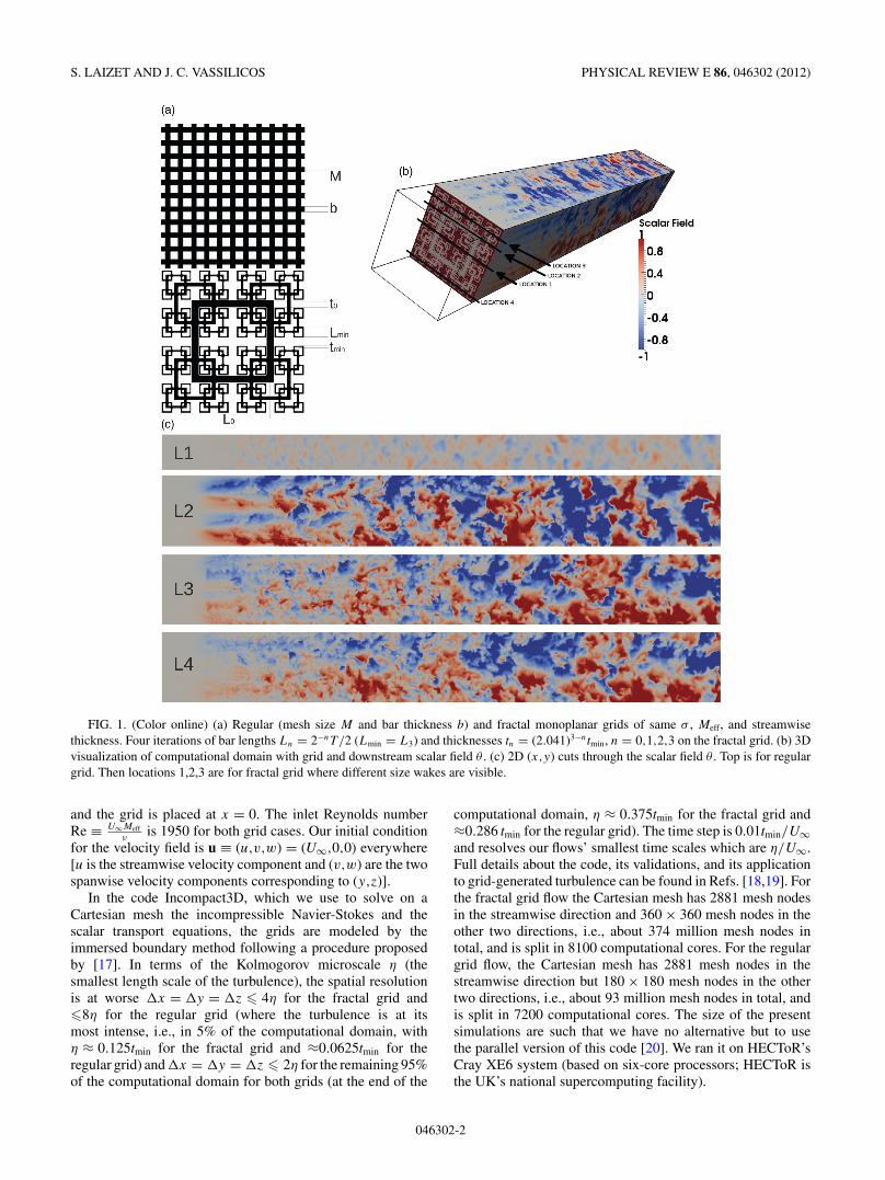
We consider two grids, one regular and one fractal [seeFig. 1(a)] of same blockage ratio σ = 0.507 (ratio of the areablocked by the grid to the area T 2 of the channel or tunnelsquare section), same thickness in the streamwise direction(normal to the grid), and same effective mesh size Meff =4T 2

LG

√1 − σ where LG is the total length of the grid when it has

been stripped of its thickness [7]. The concept of an effectivemesh size was defined and introduced by [7]; in the case of reg-ular grids, Meff equals M , the actual mesh size [see Fig. 1(a)].

Each grid is placed in a computational domain withstreamwise length Lx and spanwise extents Ly = Lz = T .For the fractal grid, Lx = 1152tmin and T = 144tmin wheretmin is the spanwise thickness of the smallest bars on the grid[see Fig. 1(a)]. For the regular grid, Lx = 576b and T = 36b

where b is the spanwise thickness of the bars on the grid [seeFig. 1(a)]. The streamwise thickness of both grids is 3tmin

and the boundary layers are laminar at the grid resulting inboundary layer thicknesses smaller than 0.5tmin; also b = 2tmin

and Meff = 6.5tmin.We assume a fluid of uniform density and kinematic

viscosity ν and inflow-outflow boundary conditions in thestreamwise direction with a uniform fluid velocity U∞ withoutturbulence as inflow condition and a one-dimensional (1D)convection equation as outflow condition. The boundary con-ditions in the two spanwise directions are periodic. Definingx ≡ (x,y,z) to be spatial coordinates in the streamwise (x)and two spanwise directions, the inflow is at x = −14Meff

046302-11539-3755/2012/86(4)/046302(5) ©2012 American Physical Society

S. LAIZET AND J. C. VASSILICOS PHYSICAL REVIEW E 86, 046302 (2012)

FIG. 1. (Color online) (a) Regular (mesh size M and bar thickness b) and fractal monoplanar grids of same σ , Meff, and streamwisethickness. Four iterations of bar lengths Ln = 2−nT /2 (Lmin = L3) and thicknesses tn = (2.041)3−ntmin, n = 0,1,2,3 on the fractal grid. (b) 3Dvisualization of computational domain with grid and downstream scalar field θ . (c) 2D (x,y) cuts through the scalar field θ . Top is for regulargrid. Then locations 1,2,3 are for fractal grid where different size wakes are visible.

and the grid is placed at x = 0. The inlet Reynolds numberRe ≡ U∞Meff

νis 1950 for both grid cases. Our initial condition

for the velocity field is u ≡ (u,v,w) = (U∞,0,0) everywhere[u is the streamwise velocity component and (v,w) are the twospanwise velocity components corresponding to (y,z)].

In the code Incompact3D, which we use to solve on aCartesian mesh the incompressible Navier-Stokes and thescalar transport equations, the grids are modeled by theimmersed boundary method following a procedure proposedby [17]. In terms of the Kolmogorov microscale η (thesmallest length scale of the turbulence), the spatial resolutionis at worse �x = �y = �z � 4η for the fractal grid and�8η for the regular grid (where the turbulence is at itsmost intense, i.e., in 5% of the computational domain, withη ≈ 0.125tmin for the fractal grid and ≈0.0625tmin for theregular grid) and �x = �y = �z � 2η for the remaining 95%of the computational domain for both grids (at the end of the

computational domain, η ≈ 0.375tmin for the fractal grid and≈0.286 tmin for the regular grid). The time step is 0.01tmin/U∞and resolves our flows’ smallest time scales which are η/U∞.Full details about the code, its validations, and its applicationto grid-generated turbulence can be found in Refs. [18,19]. Forthe fractal grid flow the Cartesian mesh has 2881 mesh nodesin the streamwise direction and 360 × 360 mesh nodes in theother two directions, i.e., about 374 million mesh nodes intotal, and is split in 8100 computational cores. For the regulargrid flow, the Cartesian mesh has 2881 mesh nodes in thestreamwise direction but 180 × 180 mesh nodes in the othertwo directions, i.e., about 93 million mesh nodes in total, andis split in 7200 computational cores. The size of the presentsimulations are such that we have no alternative but to usethe parallel version of this code [20]. We ran it on HECToR’sCray XE6 system (based on six-core processors; HECToR isthe UK’s national supercomputing facility).

046302-2

FRACTAL SPACE-SCALE UNFOLDING MECHANISM FOR . . . PHYSICAL REVIEW E 86, 046302 (2012)

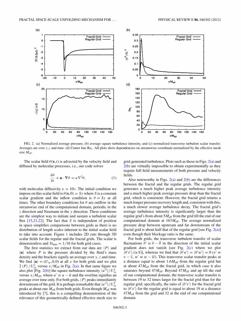
FIG. 2. (a) Normalized average pressure, (b) average square turbulence intensity, and (c) normalized transverse turbulent scalar transfer.Averages are over y,z and time. (d) Center line Reλ. All plots show dependencies on streamwise coordinate normalized by the effective meshsize Meff.

The scalar field θ (x,t) is advected by the velocity field anddiffused by molecular processes, i.e., our code solves

∂θ

∂t+ u · ∇θ = κ∇2θ, (1)

with molecular diffusivity κ = 10ν. The initial condition weimpose on this scalar field is θ (x,0) = Sy where S is a constantscalar gradient and the inflow condition is θ = Sy at alltimes. The other boundary conditions for θ are outflow in thestreamwise end of the computational domain, periodic in thez direction and Neumann in the y direction. These conditionsare the simplest way to initiate and sustain a turbulent scalarflux [15,21,22]. The fact that S is independent of positionin space simplifies comparisons between grids as there is nodistribution of length scales inherent to the initial scalar fieldto take into account. Figure 1 includes 2D cuts through 3Dscalar fields for the regular and the fractal grids. The scalar isdimensionless and Stmin = 1/16 for both grid cases.

The first statistics we extract from our data are 〈P 〉 and〈u〉 where P is the pressure divided by the fluid’s massdensity and the brackets signify an average over y, z and time.We find 〈u〉 = (U∞,0,0) at all x for both grids and we plot2 〈P 〉 /U 2

∞ versus x/Meff in Fig. 2(a). In that same figure wealso plot [Fig. 2(b)] the square turbulence intensity 〈u′2〉/U 2

∞versus x/Meff, where u′ ≡ u − u and the overline signifies anaverage over time only. For both grids, 〈P 〉 peaks immediatelydownstream of the grid. It is perhaps remarkable that 〈u′2〉/U 2

∞peaks at about one Meff from both grids. Even though Meff wasintroduced by [7], this is a compelling demonstration of therelevance of this geometrically defined effective mesh size to

grid-generated turbulence. Plots such as those in Figs. 2(a) and2(b) are virtually impossible to obtain experimentally as theyrequire full field measurements of both pressure and velocityfields.

Also noteworthy in Figs. 2(a) and 2(b) are the differencesbetween the fractal and the regular grids. The regular gridgenerates a much higher peak average turbulence intensityand a much higher peak average pressure drop than the fractalgrid, which is consistent. However, the fractal grid returns amuch longer pressure recovery length and, consistent with this,a much slower average turbulence decay. The fractal grid’saverage turbulence intensity is significantly larger than theregular grid’s from about 5Meff from the grid till the end of ourcomputational domain at 163Meff. The average normalizedpressure drop between upstream and far downstream of thefractal grid is about half that of the regular grid [see Fig. 2(a)]even though their blockage ratio is the same.

For both grids, the transverse turbulent transfer of scalarfluctuations θ ′ ≡ θ − θ in the direction of the initial scalargradient does not vanish [see Fig. 2(c) where we plot〈θ ′v′〉/(κS)], whereas we find that 〈θ ′u′〉 = 〈θ ′w′〉 = 0 (v′ ≡v − v, w′ ≡ w − w). This transverse scalar transfer peaks ata distance equal to about 1.6Meff from the regular grid butat about 47Meff from the fractal grid, in which case it alsosaturates beyond 47Meff. Beyond 47Meff and up till the endof our computational domain, the transverse scalar transfer isbetween 19 to 32 times larger for the fractal grid than for theregular grid; specifically, the ratio of 〈θ ′v′〉 for the fractal gridto 〈θ ′v′〉 for the regular grid is equal to about 19 at a distance47Meff from the grid and 32 at the end of our computationaldomain.

046302-3

S. LAIZET AND J. C. VASSILICOS PHYSICAL REVIEW E 86, 046302 (2012)

Along the center line y = z = T/2, the time-averaged θ ′v′behaves very much like 〈θ ′v′〉 for both grids. Along thatcenter line, the local Taylor length-scale Reynolds number

Reλ ≡√

u′2λ/ν [the Taylor length scale λ is defined by

λ2 ≡ u′2/( ∂u′∂x

)2] peaks for both grids at the distance from thegrid where the transverse scalar transfer peaks [see Fig. 2(d)].The streamwise location of this peak requires another lengthscale, different from Meff, to be explained, namely the wake-interaction length scale x∗ introduced by [8].

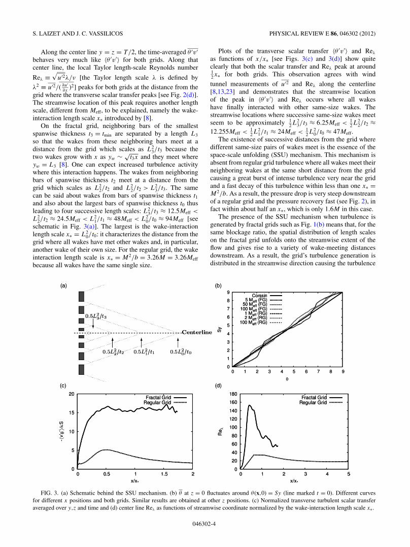
On the fractal grid, neighboring bars of the smallestspanwise thickness t3 = tmin are separated by a length L3

so that the wakes from these neighboring bars meet at adistance from the grid which scales as L2

3/t3 because thetwo wakes grow with x as yw ∼ √

t3x and they meet whereyw = L3 [8]. One can expect increased turbulence activitywhere this interaction happens. The wakes from neighboringbars of spanwise thickness t2 meet at a distance from thegrid which scales as L2

2/t2 and L22/t2 > L2

3/t3. The samecan be said about wakes from bars of spanwise thickness t1and also about the largest bars of spanwise thickness t0 thusleading to four successive length scales: L2

3/t3 ≈ 12.5Meff <

L22/t2 ≈ 24.5Meff < L2

1/t1 ≈ 48Meff < L20/t0 ≈ 94Meff [see

schematic in Fig. 3(a)]. The largest is the wake-interactionlength scale x∗ = L2

0/t0: it characterizes the distance from thegrid where all wakes have met other wakes and, in particular,another wake of their own size. For the regular grid, the wakeinteraction length scale is x∗ = M2/b = 3.26M = 3.26Meff

because all wakes have the same single size.

Plots of the transverse scalar transfer 〈θ ′v′〉 and Reλ

as functions of x/x∗ [see Figs. 3(c) and 3(d)] show quiteclearly that both the scalar transfer and Reλ peak at around12x∗ for both grids. This observation agrees with wind

tunnel measurements of u′2 and Reλ along the centerline[8,13,23] and demonstrates that the streamwise locationof the peak in 〈θ ′v′〉 and Reλ occurs where all wakeshave finally interacted with other same-size wakes. Thestreamwise locations where successive same-size wakes meetseem to be approximately 1

2L23/t3 ≈ 6.25Meff < 1

2L22/t2 ≈

12.255Meff < 12L2

1/t1 ≈ 24Meff < 12L2

0/t0 ≈ 47Meff.The existence of successive distances from the grid where

different same-size pairs of wakes meet is the essence of thespace-scale unfolding (SSU) mechanism. This mechanism isabsent from regular grid turbulence where all wakes meet theirneighboring wakes at the same short distance from the gridcausing a great burst of intense turbulence very near the gridand a fast decay of this turbulence within less than one x∗ =M2/b. As a result, the pressure drop is very steep downstreamof a regular grid and the pressure recovery fast (see Fig. 2), infact within about half an x∗, which is only 1.6M in this case.

The presence of the SSU mechanism when turbulence isgenerated by fractal grids such as Fig. 1(b) means that, for thesame blockage ratio, the spatial distribution of length scaleson the fractal grid unfolds onto the streamwise extent of theflow and gives rise to a variety of wake-meeting distancesdownstream. As a result, the grid’s turbulence generation isdistributed in the streamwise direction causing the turbulence

FIG. 3. (a) Schematic behind the SSU mechanism. (b) θ at z = 0 fluctuates around θ (x,0) = Sy (line marked t = 0). Different curvesfor different x positions and both grids. Similar results are obtained at other z positions. (c) Normalized transverse turbulent scalar transferaveraged over y,z and time and (d) center line Reλ as functions of streamwise coordinate normalized by the wake-interaction length scale x∗.

046302-4

FRACTAL SPACE-SCALE UNFOLDING MECHANISM FOR . . . PHYSICAL REVIEW E 86, 046302 (2012)

to be less and the pressure drop smaller very near the grid bycomparison to a same blockage regular grid, but also causing amuch longer pressure recovery and a much slower turbulencedecay in multiples of Meff. In multiples of x∗, however, thepressure recovery and turbulence decay distances remain ofthe order of x∗ as in the regular grid case, but x∗/Meff is oneorder of magnitude larger for the fractal grid.

The SSU mechanism can also explain the scalar transferenhancement caused by the fractal grid. We find for bothgrids that θ ≈ Sy + θr where θr is a randomly fluctuatingvariable around a constant [see Fig. 3(b); this is a non-trivial result reminiscent of one by [21] for homogeneousisotropic turbulence, see also [24]]. In our computations,advection dominates over molecular diffusion in Eq. (1),and we can therefore write θ (x0,0) ≈ θ (x,t) where x = x0 +∫ t

0 u(x(τ ),τ )dτ . It follows that θ ′(x,t) ≈ Sy0 − Sy − θr andtherefore θ ′v′ ≈ −S(y − y0)v′ where (y − y0)v′ is a turbulentdiffusivity.

From a Lagrangian viewpoint, therefore, one can see howthe SSU mechanism can increase turbulent diffusivity andthereby scalar transfer. Imagine a fluid element starting offnear the grid at a y = y0 in one of the smallest wakes. Inthe case of the regular grid, this fluid element will travelinside this wake and perhaps meet another wake of the samesize and its y coordinate will therefore predominantly remainclose to y0. However, in the case of the fractal grid, thefluid element will have a chance of jumping into a largerwake as it travels downstream, and then an even larger oneagain, each time encountering a turbulence with a larger

eddy turnover length scale. As a result, y − y0 will be muchlarger than for the regular grid for many fluid elementsand so will turbulent diffusion and scalar transfer. The SSUmechanism also distributes turbulent eddy length scales alongthe streamwise direction, in increasing size from near the gridto about 1

2x∗ at which point all wake pairs of all sizes have met.This is also the region where the scalar transfer increases, andit remains constant and larger than the scalar transfer of theregular grid by an order of magnitude beyond that point. Notethat the argument in this and the previous paragraphs requireshigh Peclet number in order to write θ ′v′ ≈ −S(y − y0)v′ andhigh Reynolds number for the wakes to be turbulent but makesno assumption on the Schmidt or Prandtl number.

The SSU mechanism has its root cause in the multiscalespace-scale structure of the fractal grid and therefore maybe expected to be present with more or less effect in awide range of turbulent flows originating from trees, forests,mountains, coral reefs, rough sea or riverbeds, and coastlinesall of which have their own multiscale or fractal structure.The SSU mechanism may, for example, play a crucial rolein the fast propagation of forest fires. We have shown thatthis mechanism can cause enhancements of scalar transfer andturbulent diffusion of at least one order of magnitude as well asvery significant reductions in pressure drop and power losses.Applying this mechanism to energy-efficient industrial mixersand heat transfer devices has the potential to set entirely newmixing and cooling standards.

We acknowledge EPSRC Grant No. EP/H030875/1.

[1] S. Hirschberg, R. Koubek, F. Moser, and J. Schock, Chem. Eng.Res. Design 87, 524 (2009).

[2] G. F. Hewitt, Heat Exchanger Design Handbook (Begell House,New York, 1998).

[3] B. Mandelbrot, The Fractal Geometry of Nature (W. H. Freeman& Co., San Francisco, 1982).

[4] K. J. Falconer, Fractal Geometry: Mathematical Foundationsand Applications (John Wiley, Chichester, 1990).

[5] M. V. Berry, Physica D 38, 29 (1989).[6] B. Sapoval and T. Gobron, Phys. Rev. E 47, 3013 (1993).[7] D. Hurst and J. C. Vassilicos, Phys. Fluids 19, 035103 (2007).[8] N. Mazellier and J. C. Vassilicos, Phys. Fluids 22, 075101

(2010).[9] K. Nagata, H. Suzuki, H. Sakai, Y. Hayase, and T. Kubo, Phys.

Scr., T 132, 014054 (2008).[10] F. Nicolleau, S. Salim, and A. Nowakowski, J. Turbulence

12(44), 1 (2011) [http://www.tandfonline.com/doi/abs/10.1080/14685248.2011.637046].

[11] G. I. Taylor, Proc. R. Soc. A 151, 421 (1935).

[12] G. Comte-Bellot and S. Corrsin, J. Fluid Mech. 48, 273 (1971).[13] Jayesh and Z. Warhaft, Phys. Fluids 4, 2292 (1992).[14] B. I. Shraiman and E. D. Siggia, Nature (London) 6787, 639

(2000).[15] Z. Warhaft, Annu. Rev. Fluid Mech. 32, 203 (2000).[16] H. Suzuki, K. Nagata, H. Sakai, and R. Ukai, Phys. Scr., T 142,

014069 (2010).[17] P. Parnaudeau, J. Carlier, D. Heitz, and E. Lamballais, Phys.

Fluids 20, 085101 (2008).[18] S. Laizet and E. Lamballais, J. Comput. Phys. 228, 5989 (2009).[19] S. Laizet and J. C. Vassilicos, Flow Turbul. Combust. 87, 673

(2011).[20] S. Laizet and N. Li, Int. J. Numer. Methods Fluids 67, 1735

(2011).[21] S. Corrsin, J. Appl. Phys. 33, 113 (1952).[22] H. K. Wiskind, J. Geophys. Res. 67, 30 (1962).[23] P. Valente and J. C. Vassilicos, J. Fluid Mech. 687, 300

(2011).[24] L. Mydlarski and Z. Warhaft, J. Fluid Mech. 358, 135 (1998).

046302-5