Embed Size (px)
Citation preview

SW Ch. 14 1/111
Introduction to Time Series Regression
and Forecasting (SW Chapter 14)
Outline
1. Time Series Data: What’s Different?
2. Using Regression Models for Forecasting
3. Lags, Differences, Autocorrelation, & Stationarity
4. Autoregressions
5. The Autoregressive – Distributed Lag (ADL) Model
6. Forecast Uncertainty and Forecast Intervals
7. Lag Length Selection: Information Criteria
8. Nonstationarity I: Trends
9. Nonstationarity II: Breaks
10. Summary
SW Ch. 14 2/111
1. Time Series Data: What’s Different?
Time series data are data collected on the same observational
unit at multiple time periods
Aggregate consumption and GDP for a country (for
example, 20 years of quarterly observations = 80
observations)
Yen/$, pound/$ and Euro/$ exchange rates (daily data for
1 year = 365 observations)
Cigarette consumption per capita in California, by year
(annual data)
SW Ch. 14 3/111
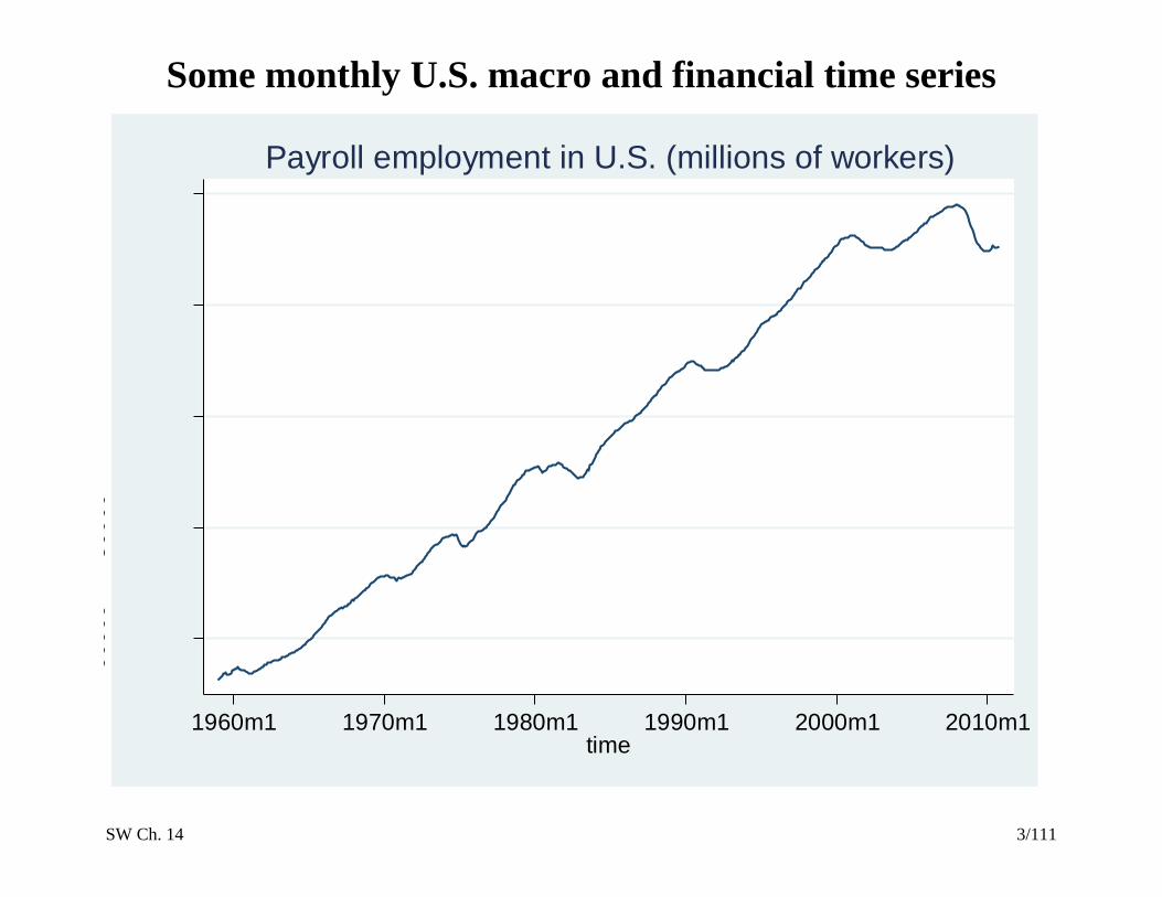
Some monthly U.S. macro and financial time series 6
00
00
800
00
100
00
01
20
00
01
40
00
0
Tota
l N
on
farm
Pa
yro
lls: A
ll E
mplo
ye
es
1960m1 1970m1 1980m1 1990m1 2000m1 2010m1time
Payroll employment in U.S. (millions of workers)

SW Ch. 14 4/111
10.8
11
11.2
11.4
11.6
11.8
lem
p
1960m1 1970m1 1980m1 1990m1 2000m1 2010m1time
Payroll employment, logs
SW Ch. 14 5/111
-1-.
50
.51
1.5
dle
mp
1960m1 1970m1 1980m1 1990m1 2000m1 2010m1time
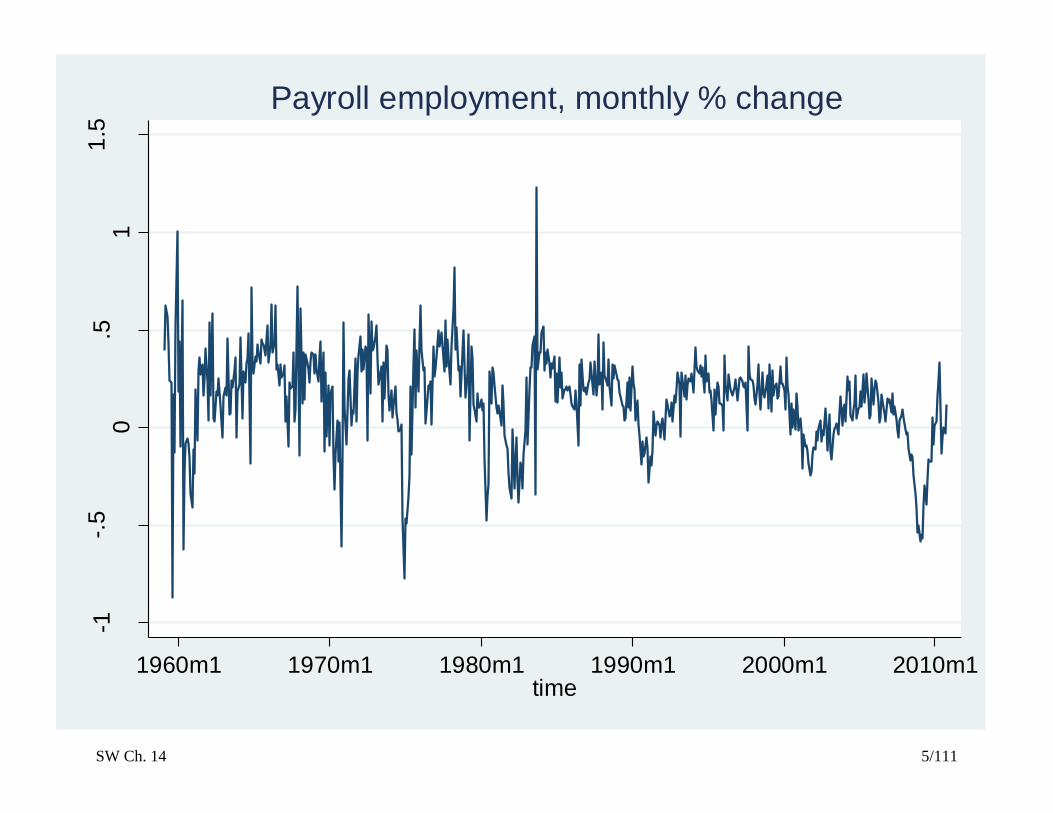
Payroll employment, monthly % change

SW Ch. 14 6/111
46
81
01
2
Civ
ilian
Une
mplo
ym
ent R
ate
1960m1 1970m1 1980m1 1990m1 2000m1 2010m1time
Civilian unemployment rate, U.S.
SW Ch. 14 7/111
-50
51
01
5
infc
pi1
2
1960m1 1970m1 1980m1 1990m1 2000m1 2010m1time
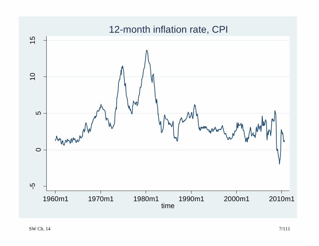
12-month inflation rate, CPI

SW Ch. 14 8/111
05
10
15
20
3-M
on
th T
rea
sury
Bill
: S
econ
da
ry M
ark
et R
ate
1960m1 1970m1 1980m1 1990m1 2000m1 2010m1time
Interest rate on 90-day Treasury bills

SW Ch. 14 9/111
05
10
15
10-Y
ear
Tre
asu
ry C
on
sta
nt M
atu
rity
Rate
1960m1 1970m1 1980m1 1990m1 2000m1 2010m1time
Yield on 10-year Treasury bonds
SW Ch. 14 10/111
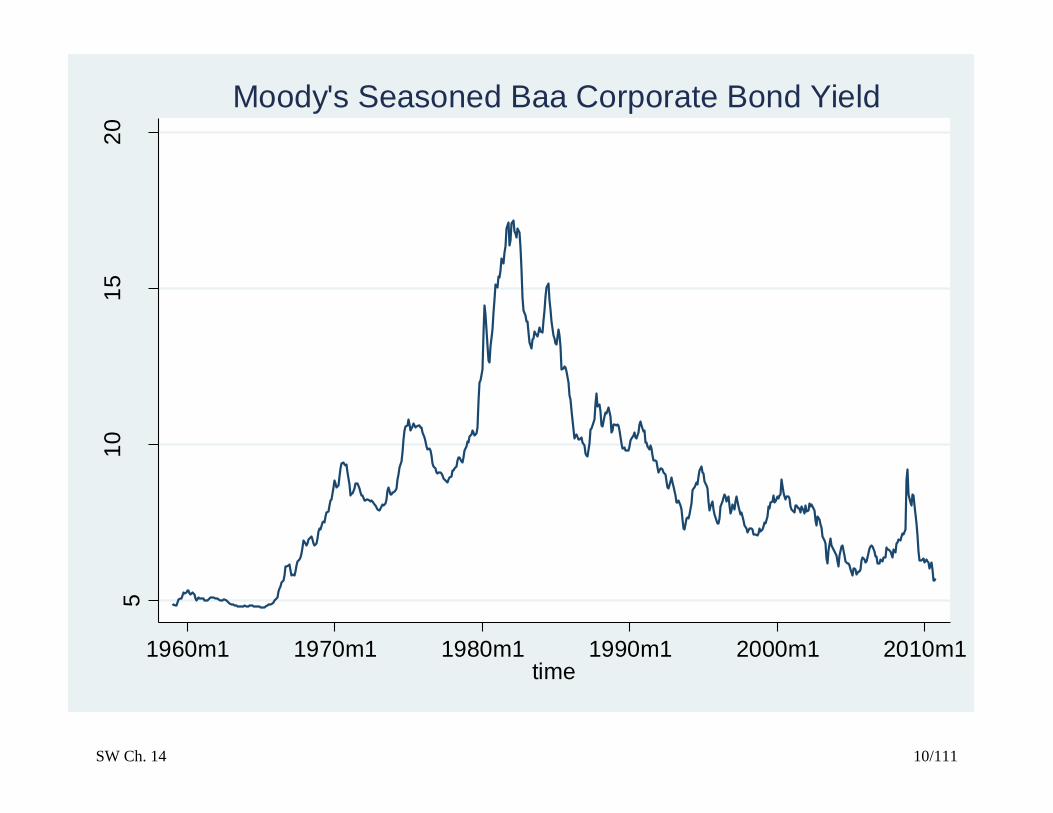
51
01
52
0
Mo
od
y's
Se
aso
ne
d B
aa
Corp
ora
te B
ond
Yie
ld
1960m1 1970m1 1980m1 1990m1 2000m1 2010m1time
Moody's Seasoned Baa Corporate Bond Yield

SW Ch. 14 11/111
02
46
baa
_r1
0
1960m1 1970m1 1980m1 1990m1 2000m1 2010m1time
Yield spread, BAA corporate minus 10-year Treasuries

SW Ch. 14 12/111
A daily U.S. financial time series:
SW Ch. 14 13/111
Some uses of time series data
Forecasting (SW Ch. 14)
Estimation of dynamic causal effects (SW Ch. 15)
o If the Fed increases the Federal Funds rate now, what
will be the effect on the rates of inflation and
unemployment in 3 months? In 12 months?
o What is the effect over time on cigarette consumption
of a hike in the cigarette tax?
Modeling risks, which is used in financial markets (one
aspect of this, modeling changing variances and “volatility
clustering,” is discussed in SW Ch. 16)
Applications outside of economics include environmental
and climate modeling, engineering (system dynamics),
computer science (network dynamics),…

SW Ch. 14 14/111
Time series data raises new technical issues
Time lags
Correlation over time (serial correlation, a.k.a.
autocorrelation – which we encountered in panel data)
Calculation of standard errors when the errors are serially
correlated
A good way to learn about time series data is to
investigate it yourself! A great source for U.S. macro time
series data, and some international data, is the Federal
Reserve Bank of St. Louis’s FRED database.
SW Ch. 14 15/111
2. Using Regression Models for Forecasting
(SW Section 14.1)
Forecasting and estimation of causal effects are quite
different objectives.
For forecasting,
o 2R matters (a lot!)
o Omitted variable bias isn’t a problem!
o We won’t worry about interpreting coefficients in
forecasting models – no need to estimate causal effects
if all you want to do is forecast!
o External validity is paramount: the model estimated
using historical data must hold into the (near) future
SW Ch. 14 16/111
3. Introduction to Time Series Data
and Serial Correlation
(SW Section 14.2)
Time series basics:
A. Notation
B. Lags, first differences, and growth rates
C. Autocorrelation (serial correlation)
D. Stationarity

SW Ch. 14 17/111
A. Notation
Yt = value of Y in period t.
Data set: {Y1,…,YT} are T observations on the time series
variable Y
We consider only consecutive, evenly-spaced
observations (for example, monthly, 1960 to 1999, no
missing months) (missing and unevenly spaced data
introduce technical complications)
SW Ch. 14 18/111
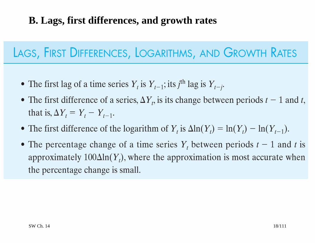
B. Lags, first differences, and growth rates

SW Ch. 14 19/111
Example: Quarterly rate of inflation at an annual rate (U.S.)
CPI = Consumer Price Index (Bureau of Labor Statistics)
CPI in the first quarter of 2004 (2004:I) = 186.57
CPI in the second quarter of 2004 (2004:II) = 188.60
Percentage change in CPI, 2004:I to 2004:II
= 188.60 186.57
100186.57
= 2.03
100186.57
= 1.088%
Percentage change in CPI, 2004:I to 2004:II, at an annual
rate = 41.088 = 4.359% 4.4% (percent per year)
Like interest rates, inflation rates are (as a matter of
convention) reported at an annual rate.
Using the logarithmic approximation to percent changes
yields 4100[log(188.60) – log(186.57)] = 4.329%

SW Ch. 14 20/111
Example: US CPI inflation – its first lag and its change
SW Ch. 14 21/111
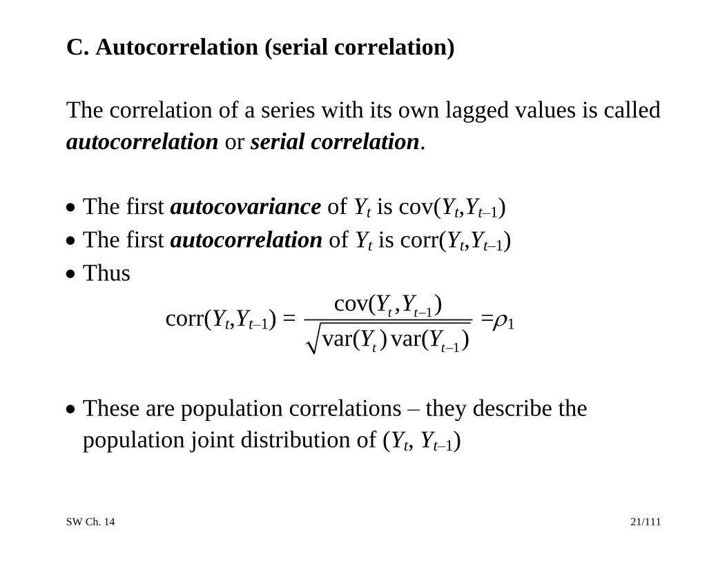
C. Autocorrelation (serial correlation)
The correlation of a series with its own lagged values is called
autocorrelation or serial correlation.
The first autocovariance of Yt is cov(Yt,Yt–1)
The first autocorrelation of Yt is corr(Yt,Yt–1)
Thus
corr(Yt,Yt–1) = 1
1
cov( , )
var( ) var( )
t t
t t
Y Y
Y Y
=1
These are population correlations – they describe the
population joint distribution of (Yt, Yt–1)

SW Ch. 14 22/111

SW Ch. 14 23/111
Sample autocorrelations
The jth
sample autocorrelation is an estimate of the jth
population autocorrelation:
ˆj =
cov( , )
var( )
t t j
t
Y Y
Y
where
cov( , )t t jY Y = 1, 1,
1
1( )( )
T
t j T t j T j
t j
Y Y Y YT
where 1,j TY is the sample average of Yt computed over
observations t = j+1,…,T. NOTE:
o The summation is over t=j+1 to T (why?)
o The divisor is T, not T – j (this is the conventional
definition used for time series data)

SW Ch. 14 24/111
Example: Autocorrelations of:
(1) the quarterly rate of U.S. inflation
(2) the quarter-to-quarter change in the quarterly rate of
inflation
SW Ch. 14 25/111
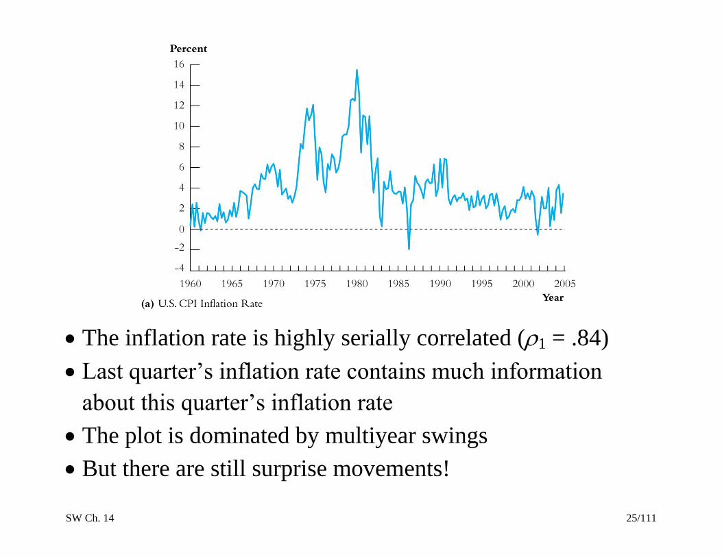
The inflation rate is highly serially correlated (1 = .84)
Last quarter’s inflation rate contains much information
about this quarter’s inflation rate
The plot is dominated by multiyear swings
But there are still surprise movements!
SW Ch. 14 26/111
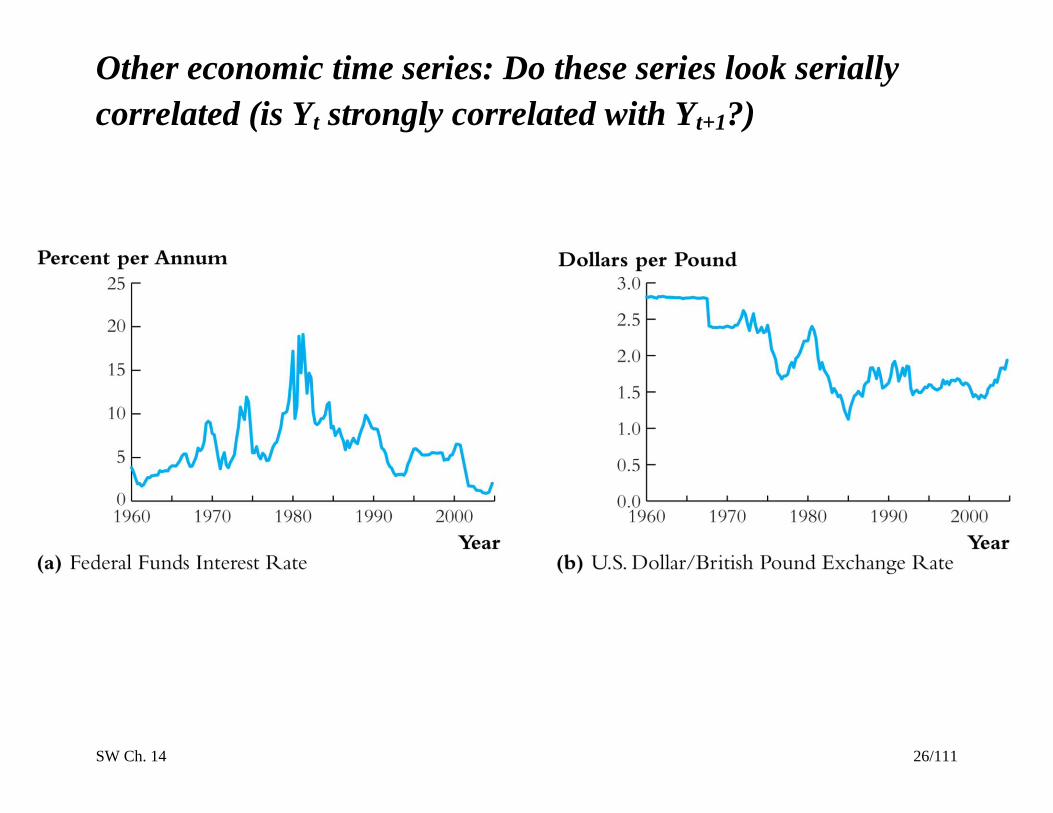
Other economic time series: Do these series look serially
correlated (is Yt strongly correlated with Yt+1?)

SW Ch. 14 27/111
Other economic time series, ctd:

SW Ch. 14 28/111
D. Stationarity
Stationarity says that history is relevant. Stationarity is a key
requirement for external validity of time series regression.
For now, assume that Yt is stationary (we return to this later).

SW Ch. 14 29/111
4. Autoregressions
(SW Section 14.3)
A natural starting point for a forecasting model is to use past
values of Y (that is, Yt–1, Yt–2,…) to forecast Yt.
An autoregression is a regression model in which Yt is
regressed against its own lagged values.
The number of lags used as regressors is called the order
of the autoregression.
o In a first order autoregression, Yt is regressed against
Yt–1
o In a pth
order autoregression, Yt is regressed against
Yt–1,Yt–2,…,Yt–p.
SW Ch. 14 30/111
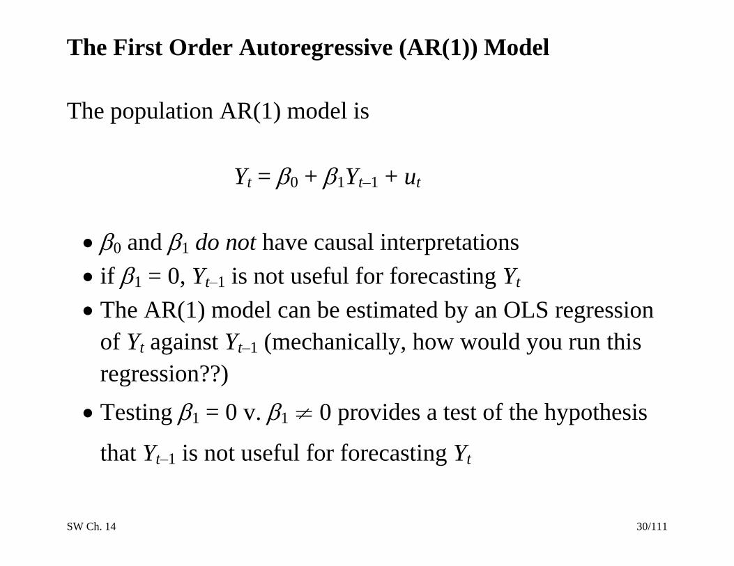
The First Order Autoregressive (AR(1)) Model
The population AR(1) model is
Yt = 0 + 1Yt–1 + ut
0 and 1 do not have causal interpretations
if 1 = 0, Yt–1 is not useful for forecasting Yt
The AR(1) model can be estimated by an OLS regression
of Yt against Yt–1 (mechanically, how would you run this
regression??)
Testing 1 = 0 v. 1 0 provides a test of the hypothesis
that Yt–1 is not useful for forecasting Yt
SW Ch. 14 31/111
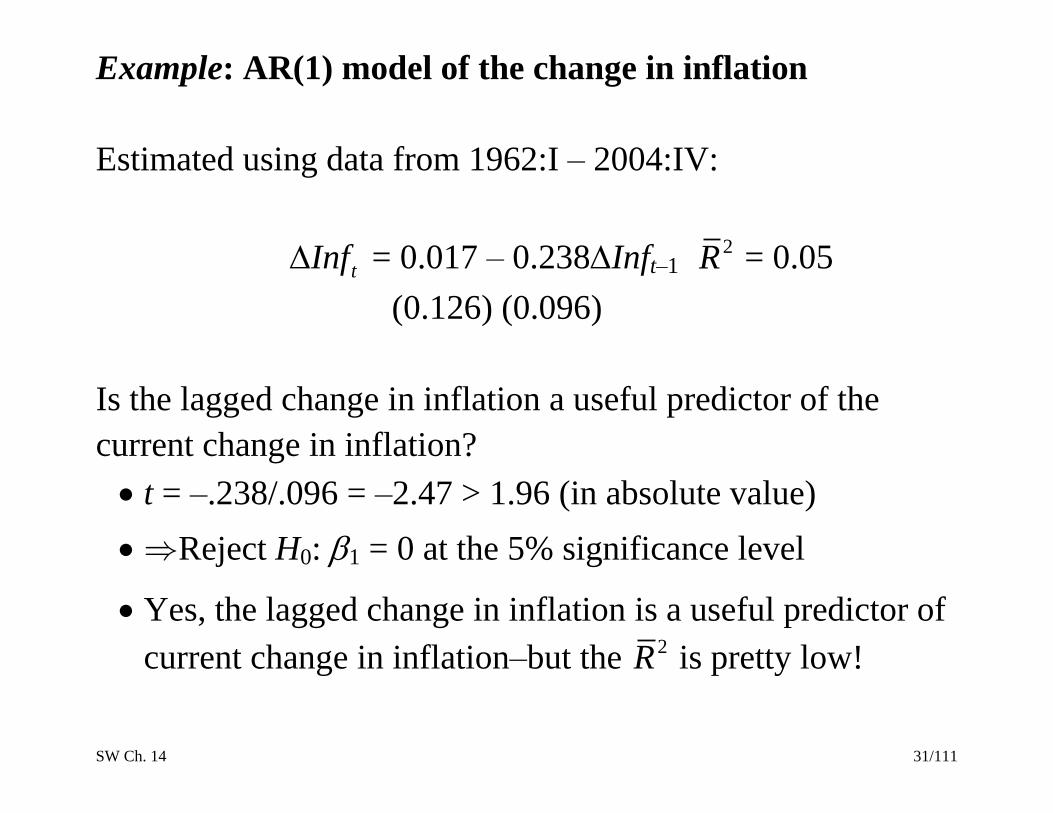
Example: AR(1) model of the change in inflation
Estimated using data from 1962:I – 2004:IV:
tInf = 0.017 – 0.238Inft–1 2R = 0.05
(0.126) (0.096)
Is the lagged change in inflation a useful predictor of the
current change in inflation?
t = –.238/.096 = –2.47 > 1.96 (in absolute value)
Reject H0: 1 = 0 at the 5% significance level
Yes, the lagged change in inflation is a useful predictor of
current change in inflation–but the 2R is pretty low!
SW Ch. 14 32/111
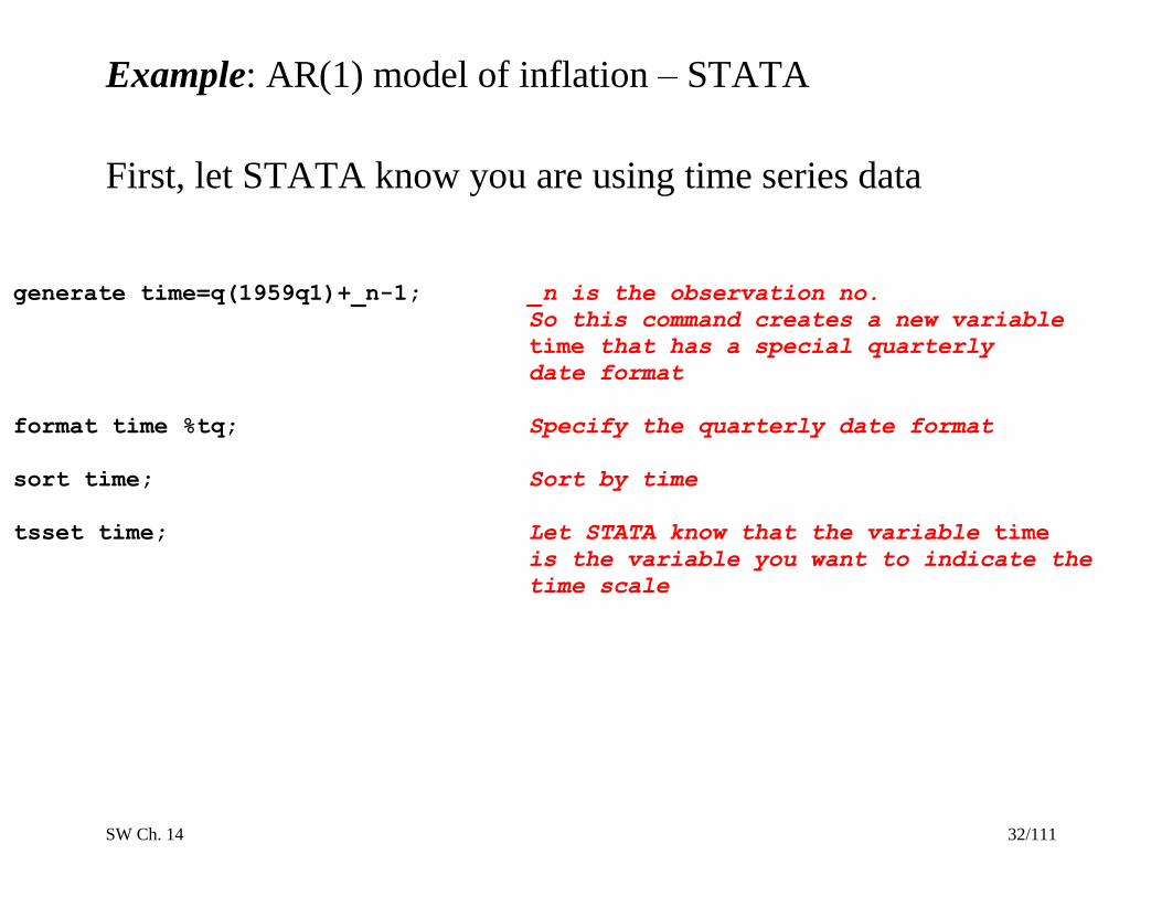
Example: AR(1) model of inflation – STATA
First, let STATA know you are using time series data
generate time=q(1959q1)+_n-1; _n is the observation no.
So this command creates a new variable
time that has a special quarterly
date format
format time %tq; Specify the quarterly date format
sort time; Sort by time
tsset time; Let STATA know that the variable time
is the variable you want to indicate the
time scale

SW Ch. 14 33/111
Example: AR(1) model of inflation – STATA, ctd.
. gen lcpi = log(cpi); variable cpi is already in memory
. gen inf = 400*(lcpi[_n]-lcpi[_n-1]); quarterly rate of inflation at an
annual rate
This creates a new variable, inf, the “nth” observation of which is 400
times the difference between the nth observation on lcpi and the “n-1”th
observation on lcpi, that is, the first difference of lcpi
compute first 8 sample autocorrelations
. corrgram inf if tin(1960q1,2004q4), noplot lags(8);
LAG AC PAC Q Prob>Q
-----------------------------------------
1 0.8359 0.8362 127.89 0.0000
2 0.7575 0.1937 233.5 0.0000
3 0.7598 0.3206 340.34 0.0000
4 0.6699 -0.1881 423.87 0.0000
5 0.5964 -0.0013 490.45 0.0000
6 0.5592 -0.0234 549.32 0.0000
7 0.4889 -0.0480 594.59 0.0000
8 0.3898 -0.1686 623.53 0.0000
if tin(1962q1,2004q4) is STATA time series syntax for using only observations
between 1962q1 and 1999q4 (inclusive). The “tin(.,.)” option requires defining
the time scale first, as we did above
SW Ch. 14 34/111
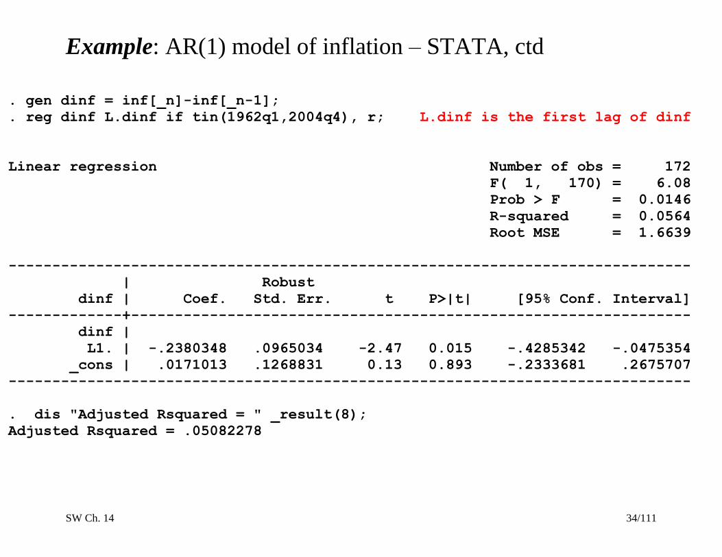
Example: AR(1) model of inflation – STATA, ctd
. gen dinf = inf[_n]-inf[_n-1];
. reg dinf L.dinf if tin(1962q1,2004q4), r; L.dinf is the first lag of dinf
Linear regression Number of obs = 172
F( 1, 170) = 6.08
Prob > F = 0.0146
R-squared = 0.0564
Root MSE = 1.6639
------------------------------------------------------------------------------
| Robust
dinf | Coef. Std. Err. t P>|t| [95% Conf. Interval]
-------------+----------------------------------------------------------------
dinf |
L1. | -.2380348 .0965034 -2.47 0.015 -.4285342 -.0475354
_cons | .0171013 .1268831 0.13 0.893 -.2333681 .2675707
------------------------------------------------------------------------------
. dis "Adjusted Rsquared = " _result(8);
Adjusted Rsquared = .05082278
SW Ch. 14 35/111
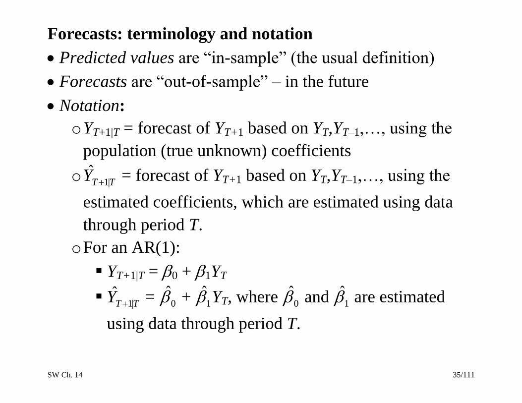
Forecasts: terminology and notation
Predicted values are “in-sample” (the usual definition)
Forecasts are “out-of-sample” – in the future
Notation:
o YT+1|T = forecast of YT+1 based on YT,YT–1,…, using the
population (true unknown) coefficients
o 1|ˆT TY = forecast of YT+1 based on YT,YT–1,…, using the
estimated coefficients, which are estimated using data
through period T.
o For an AR(1):
YT+1|T = 0 + 1YT
1|ˆT TY = 0̂ + 1̂ YT, where 0̂ and 1̂ are estimated
using data through period T.

SW Ch. 14 36/111
Forecast errors
The one-period ahead forecast error is,
forecast error = YT+1 – 1|ˆT TY
The distinction between a forecast error and a residual is the
same as between a forecast and a predicted value:
a residual is “in-sample”
a forecast error is “out-of-sample” – the value of YT+1
isn’t used in the estimation of the regression coefficients
SW Ch. 14 37/111
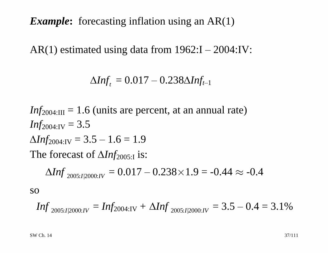
Example: forecasting inflation using an AR(1)
AR(1) estimated using data from 1962:I – 2004:IV:
tInf = 0.017 – 0.238Inft–1
Inf2004:III = 1.6 (units are percent, at an annual rate)
Inf2004:IV = 3.5
Inf2004:IV = 3.5 – 1.6 = 1.9
The forecast of Inf2005:I is:
2005: |2000:I IVInf = 0.017 – 0.2381.9 = -0.44 -0.4
so
2005: |2000:I IVInf = Inf2004:IV + 2005: |2000:I IVInf = 3.5 – 0.4 = 3.1%

SW Ch. 14 38/111
The AR(p) model: using multiple lags for forecasting
The pth
order autoregressive model (AR(p)) is
Yt = 0 + 1Yt–1 + 2Yt–2 + … + pYt–p + ut
The AR(p) model uses p lags of Y as regressors
The AR(1) model is a special case
The coefficients do not have a causal interpretation
To test the hypothesis that Yt–2,…,Yt–p do not further help
forecast Yt, beyond Yt–1, use an F-test
Use t- or F-tests to determine the lag order p
Or, better, determine p using an “information criterion”
SW Ch. 14 39/111
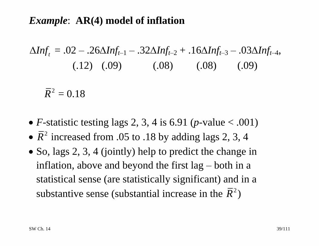
Example: AR(4) model of inflation
tInf = .02 – .26Inft–1 – .32Inft–2 + .16Inft–3 – .03Inft–4,
(.12) (.09) (.08) (.08) (.09)
2R = 0.18
F-statistic testing lags 2, 3, 4 is 6.91 (p-value < .001)
2R increased from .05 to .18 by adding lags 2, 3, 4
So, lags 2, 3, 4 (jointly) help to predict the change in
inflation, above and beyond the first lag – both in a
statistical sense (are statistically significant) and in a
substantive sense (substantial increase in the 2R )

SW Ch. 14 40/111
Example: AR(4) model of inflation – STATA
. reg dinf L(1/4).dinf if tin(1962q1,2004q4), r;
Linear regression Number of obs = 172
F( 4, 167) = 7.93
Prob > F = 0.0000
R-squared = 0.2038
Root MSE = 1.5421
------------------------------------------------------------------------------
| Robust
dinf | Coef. Std. Err. t P>|t| [95% Conf. Interval]
-------------+----------------------------------------------------------------
dinf |
L1. | -.2579205 .0925955 -2.79 0.006 -.4407291 -.0751119
L2. | -.3220302 .0805456 -4.00 0.000 -.481049 -.1630113
L3. | .1576116 .0841023 1.87 0.063 -.0084292 .3236523
L4. | -.0302685 .0930452 -0.33 0.745 -.2139649 .1534278
_cons | .0224294 .1176329 0.19 0.849 -.2098098 .2546685
------------------------------------------------------------------------------
NOTES
L(1/4).dinf is A convenient way to say “use lags 1–4 of dinf as regressors”
L1,…,L4 refer to the first, second,… 4th lags of dinf

SW Ch. 14 41/111
Example: AR(4) model of inflation – STATA, ctd.
. dis "Adjusted Rsquared = " _result(8); result(8) is the rbar-squared
Adjusted Rsquared = .18474733 of the most recently run regression
. test L2.dinf L3.dinf L4.dinf; L2.dinf is the second lag of dinf, etc.
( 1) L2.dinf = 0.0
( 2) L3.dinf = 0.0
( 3) L4.dinf = 0.0
F( 3, 147) = 6.71
Prob > F = 0.0003
SW Ch. 14 42/111
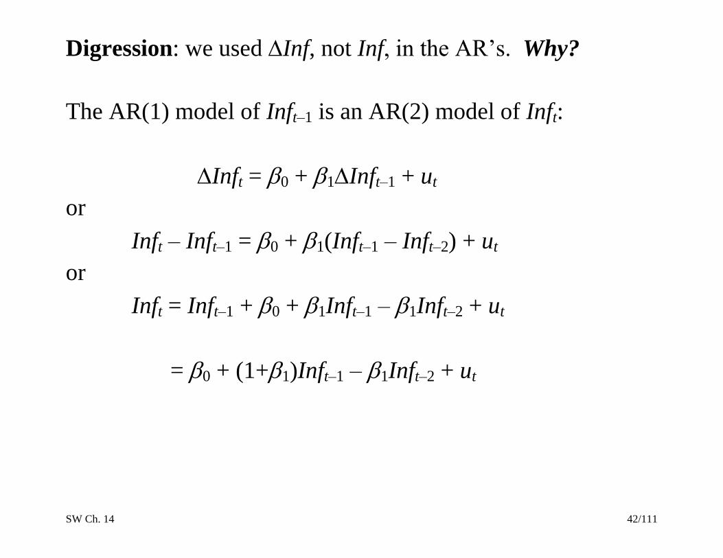
Digression: we used Inf, not Inf, in the AR’s. Why?
The AR(1) model of Inft–1 is an AR(2) model of Inft:
Inft = 0 + 1Inft–1 + ut
or
Inft – Inft–1 = 0 + 1(Inft–1 – Inft–2) + ut
or
Inft = Inft–1 + 0 + 1Inft–1 – 1Inft–2 + ut
= 0 + (1+1)Inft–1 – 1Inft–2 + ut

SW Ch. 14 43/111
So why use Inft, not Inft?
AR(1) model of Inf: Inft = 0 + 1Inft–1 + ut
AR(2) model of Inf: Inft = 0 + 1Inft + 2Inft–1 + vt
When Yt is strongly serially correlated, the OLS estimator of
the AR coefficient is biased towards zero.
In the extreme case that the AR coefficient = 1, Yt isn’t
stationary: the ut’s accumulate and Yt blows up.
If Yt isn’t stationary, the regression output can be un reliable
(this is complicated – regressions with trending variables
can be misleading, t-stats don’t have normal distributions,
etc. – more on this later)
Here, Inft is strongly serially correlated – so to keep
ourselves in a framework we understand, the regressions are
specified using Inf

SW Ch. 14 44/111
5. Time Series Regression with Additional Predictors and
the Autoregressive Distributed Lag (ADL) Model
(SW Section 14.4)
So far we have considered forecasting models that use only
past values of Y
It makes sense to add other variables (X) that might be
useful predictors of Y, above and beyond the predictive
value of lagged values of Y:
Yt = 0 + 1Yt–1 + … + pYt–p + 1Xt–1 + … + rXt–r + ut
This is an autoregressive distributed lag model with p lags
of Y and r lags of X … ADL(p,r).
SW Ch. 14 45/111
Example: Inflation and Unemployment
According to the “Phillips curve,” if unemployment is
above its equilibrium, or “natural,” rate, then the rate of
inflation will increase. That is, Inft is related to lagged
values of the unemployment rate, with a negative coefficient
The rate of unemployment at which inflation neither
increases nor decreases is often called the “Non-
Accelerating Inflation Unemployment Rate” (the NAIRU).
Is the Phillips curve found in US economic data?
Can it be exploited for forecasting inflation?
Has the U.S. Phillips curve been stable over time?
SW Ch. 14 46/111
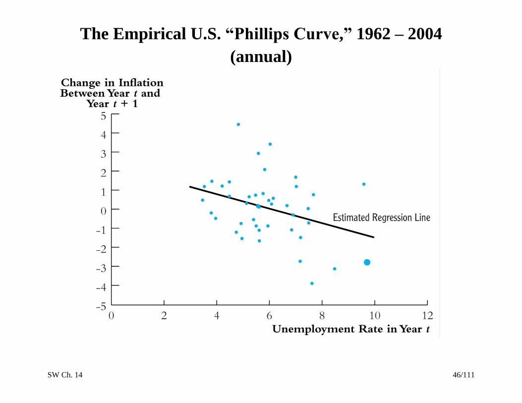
The Empirical U.S. “Phillips Curve,” 1962 – 2004
(annual)

SW Ch. 14 47/111
One definition of the NAIRU is that it is the value of u for
which Inf = 0 – the x intercept of the regression line.
SW Ch. 14 48/111
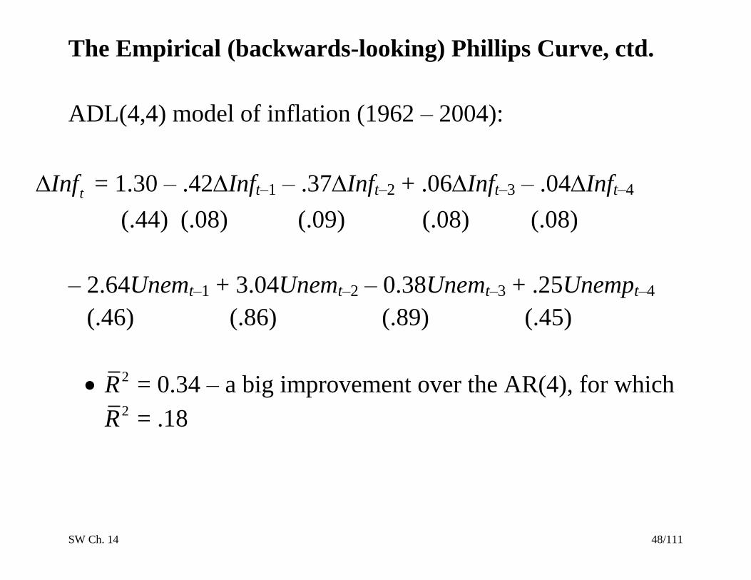
The Empirical (backwards-looking) Phillips Curve, ctd.
ADL(4,4) model of inflation (1962 – 2004):
tInf = 1.30 – .42Inft–1 – .37Inft–2 + .06Inft–3 – .04Inft–4
(.44) (.08) (.09) (.08) (.08)
– 2.64Unemt–1 + 3.04Unemt–2 – 0.38Unemt–3 + .25Unempt–4
(.46) (.86) (.89) (.45)
2R = 0.34 – a big improvement over the AR(4), for which 2R = .18

SW Ch. 14 49/111
Example: dinf and unem – STATA
. reg dinf L(1/4).dinf L(1/4).unem if tin(1962q1,2004q4), r;
Linear regression Number of obs = 172
F( 8, 163) = 8.95
Prob > F = 0.0000
R-squared = 0.3663
Root MSE = 1.3926
------------------------------------------------------------------------------
| Robust
dinf | Coef. Std. Err. t P>|t| [95% Conf. Interval]
-------------+----------------------------------------------------------------
dinf |
L1. | -.4198002 .0886973 -4.73 0.000 -.5949441 -.2446564
L2. | -.3666267 .0940369 -3.90 0.000 -.5523143 -.1809391
L3. | .0565723 .0847966 0.67 0.506 -.1108691 .2240138
L4. | -.0364739 .0835277 -0.44 0.663 -.2014098 .128462
unem |
L1. | -2.635548 .4748106 -5.55 0.000 -3.573121 -1.697975
L2. | 3.043123 .8797389 3.46 0.001 1.305969 4.780277
L3. | -.3774696 .9116437 -0.41 0.679 -2.177624 1.422685
L4. | -.2483774 .4605021 -0.54 0.590 -1.157696 .6609413
_cons | 1.304271 .4515941 2.89 0.004 .4125424 2.196
------------------------------------------------------------------------------

SW Ch. 14 50/111
Example: ADL(4,4) model of inflation – STATA, ctd.
. dis "Adjusted Rsquared = " _result(8);
Adjusted Rsquared = .33516905
. test L1.unem L2.unem L3.unem L4.unem;
( 1) L.unem = 0
( 2) L2.unem = 0
( 3) L3.unem = 0
( 4) L4.unem = 0
F( 4, 163) = 8.44 The lags of unem are significant
Prob > F = 0.0000
The null hypothesis that the coefficients on the lags of the
unemployment rate are all zero is rejected at the 1% significance
level using the F-statistic
SW Ch. 14 51/111
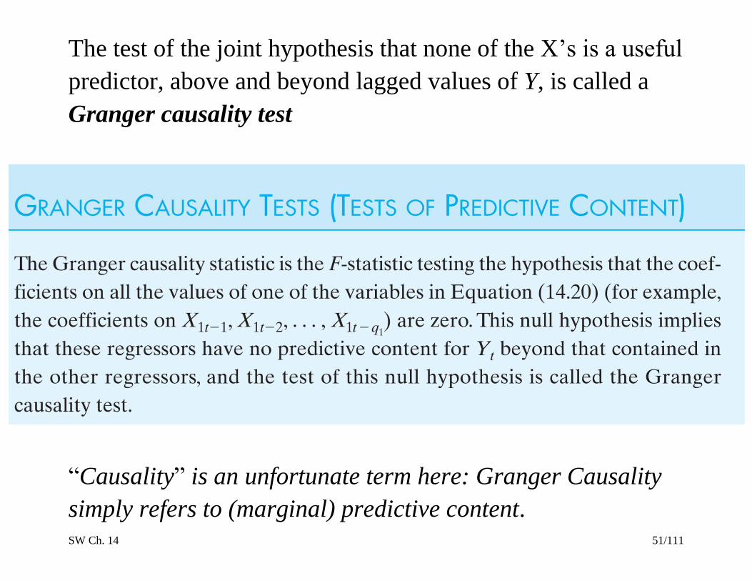
The test of the joint hypothesis that none of the X’s is a useful
predictor, above and beyond lagged values of Y, is called a
Granger causality test
“Causality” is an unfortunate term here: Granger Causality
simply refers to (marginal) predictive content.
SW Ch. 14 52/111
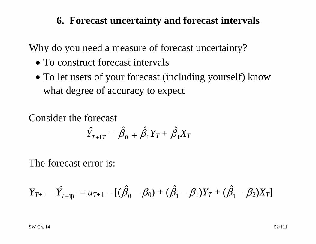
6. Forecast uncertainty and forecast intervals
Why do you need a measure of forecast uncertainty?
To construct forecast intervals
To let users of your forecast (including yourself) know
what degree of accuracy to expect
Consider the forecast
1|ˆT TY = 0̂ + 1̂ YT + 1̂ XT
The forecast error is:
YT+1 – 1|ˆT TY = uT+1 – [( 0̂ – 0) + ( 1̂ – 1)YT + ( 1̂ – 2)XT]
SW Ch. 14 53/111
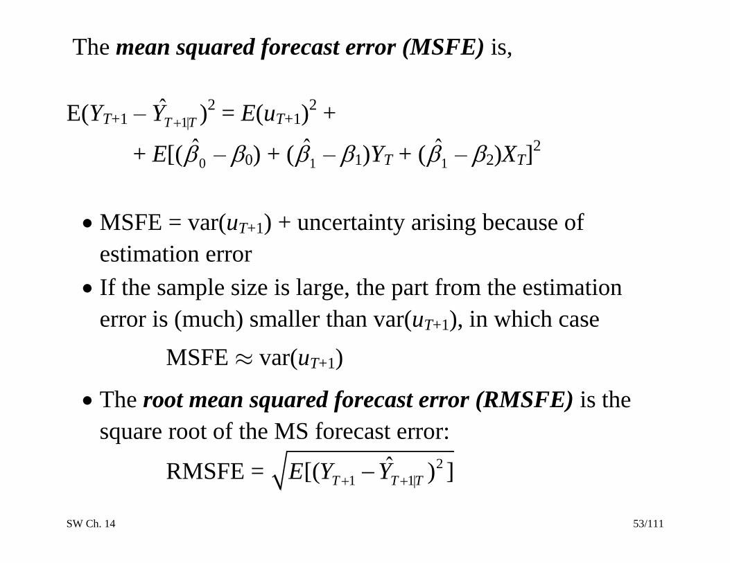
The mean squared forecast error (MSFE) is,
E(YT+1 – 1|ˆT TY )
2 = E(uT+1)
2 +
+ E[( 0̂ – 0) + ( 1̂ – 1)YT + ( 1̂ – 2)XT]2
MSFE = var(uT+1) + uncertainty arising because of
estimation error
If the sample size is large, the part from the estimation
error is (much) smaller than var(uT+1), in which case
MSFE var(uT+1)
The root mean squared forecast error (RMSFE) is the
square root of the MS forecast error:
RMSFE = 2
1 1|ˆ[( ) ]T T TE Y Y
SW Ch. 14 54/111
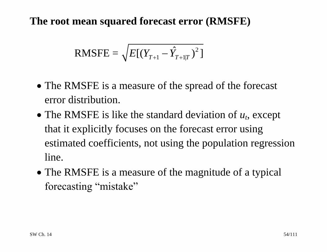
The root mean squared forecast error (RMSFE)
RMSFE = 2
1 1|ˆ[( ) ]T T TE Y Y
The RMSFE is a measure of the spread of the forecast
error distribution.
The RMSFE is like the standard deviation of ut, except
that it explicitly focuses on the forecast error using
estimated coefficients, not using the population regression
line.
The RMSFE is a measure of the magnitude of a typical
forecasting “mistake”
SW Ch. 14 55/111
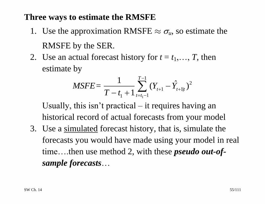
Three ways to estimate the RMSFE
1. Use the approximation RMSFE u, so estimate the
RMSFE by the SER.
2. Use an actual forecast history for t = t1,…, T, then
estimate by
MSFE= 1
12
1 1|
11
1 ˆ( )1
T
t t t
t t
Y YT t
Usually, this isn’t practical – it requires having an
historical record of actual forecasts from your model
3. Use a simulated forecast history, that is, simulate the
forecasts you would have made using your model in real
time….then use method 2, with these pseudo out-of-
sample forecasts…
SW Ch. 14 56/111
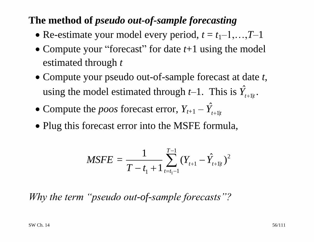
The method of pseudo out-of-sample forecasting
Re-estimate your model every period, t = t1–1,…,T–1
Compute your “forecast” for date t+1 using the model
estimated through t
Compute your pseudo out-of-sample forecast at date t,
using the model estimated through t–1. This is 1|ˆt tY .
Compute the poos forecast error, Yt+1 – 1|ˆt tY
Plug this forecast error into the MSFE formula,
MSFE = 1
12
1 1|
11
1 ˆ( )1
T
t t t
t t
Y YT t
Why the term “pseudo out-of-sample forecasts”?

SW Ch. 14 57/111
Using the RMSFE to construct forecast intervals
If uT+1 is normally distributed, then a 95% forecast interval
can be constructed as
| 1ˆT TY 1.96RMSFE
Note:
1. A 95% forecast interval is not a confidence interval (YT+1
isn’t a nonrandom coefficient, it is random!)
2. This interval is only valid if uT+1 is normal – but still
might be a reasonable approximation and is a commonly
used measure of forecast uncertainty
3. Often “67%” forecast intervals are used: RMSFE

SW Ch. 14 58/111
Example #1: The Bank of England “Fan Chart”, Feb. 2011
http://www.bankofengland.co.uk/publications/inflationreport/ir11feb.pdf
SW Ch. 14 59/111
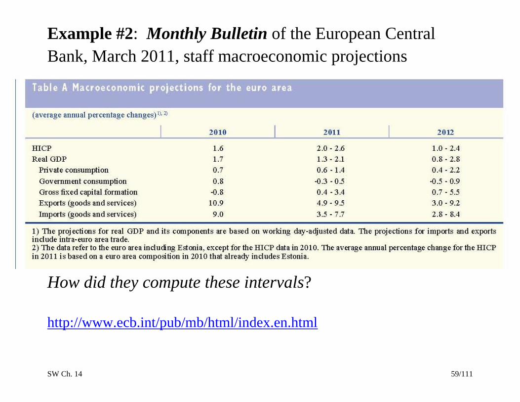
Example #2: Monthly Bulletin of the European Central
Bank, March 2011, staff macroeconomic projections
How did they compute these intervals?
http://www.ecb.int/pub/mb/html/index.en.html

SW Ch. 14 60/111
Example #3: Fed, Semiannual Report to Congress, Feb.
2010: Figure 1. Central Tendencies and Ranges of Economic
Projections, 2010-12 and over the Longer Run
How did they compute these intervals?
http://www.federalreserve.gov/boarddocs/rptcongress/annual09/default.htm

SW Ch. 14 61/111
7. Lag Length Selection Using Information Criteria
(SW Section 14.5)
How to choose the number of lags p in an AR(p)?
Omitted variable bias is irrelevant for forecasting!
You can use sequential “downward” t- or F-tests; but the
models chosen tend to be “too large” (why?)
Another – better – way to determine lag lengths is to use
an information criterion
Information criteria trade off bias (too few lags) vs.
variance (too many lags)
Two IC are the Bayes (BIC) and Akaike (AIC)…
SW Ch. 14 62/111
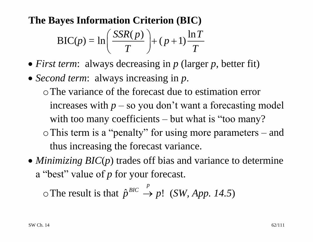
The Bayes Information Criterion (BIC)
BIC(p) = ( ) ln
ln ( 1)SSR p T
pT T
First term: always decreasing in p (larger p, better fit)
Second term: always increasing in p.
o The variance of the forecast due to estimation error
increases with p – so you don’t want a forecasting model
with too many coefficients – but what is “too many?
o This term is a “penalty” for using more parameters – and
thus increasing the forecast variance.
Minimizing BIC(p) trades off bias and variance to determine
a “best” value of p for your forecast.
o The result is that ˆ BICp p
p! (SW, App. 14.5)
SW Ch. 14 63/111
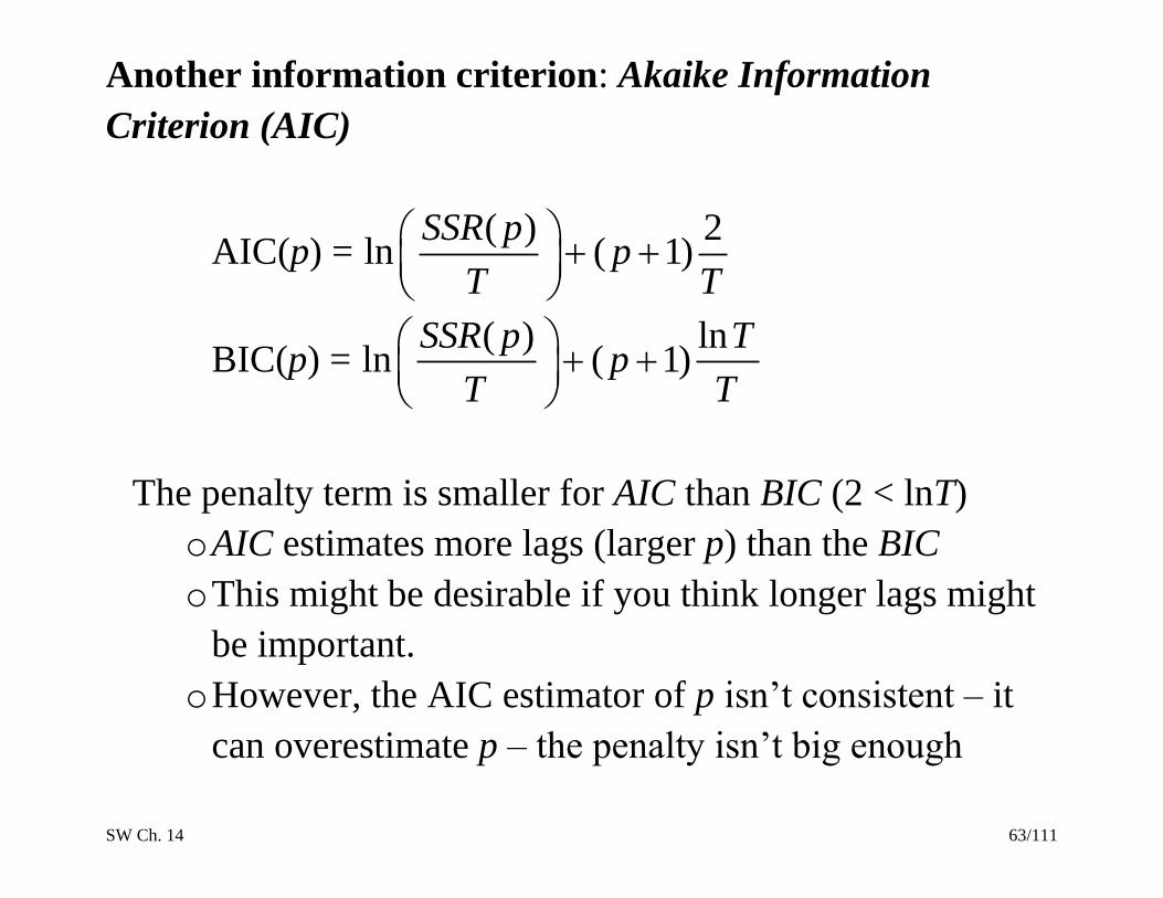
Another information criterion: Akaike Information
Criterion (AIC)
AIC(p) = ( ) 2
ln ( 1)SSR p
pT T
BIC(p) = ( ) ln
ln ( 1)SSR p T
pT T
The penalty term is smaller for AIC than BIC (2 < lnT)
o AIC estimates more lags (larger p) than the BIC
o This might be desirable if you think longer lags might
be important.
o However, the AIC estimator of p isn’t consistent – it
can overestimate p – the penalty isn’t big enough
SW Ch. 14 64/111
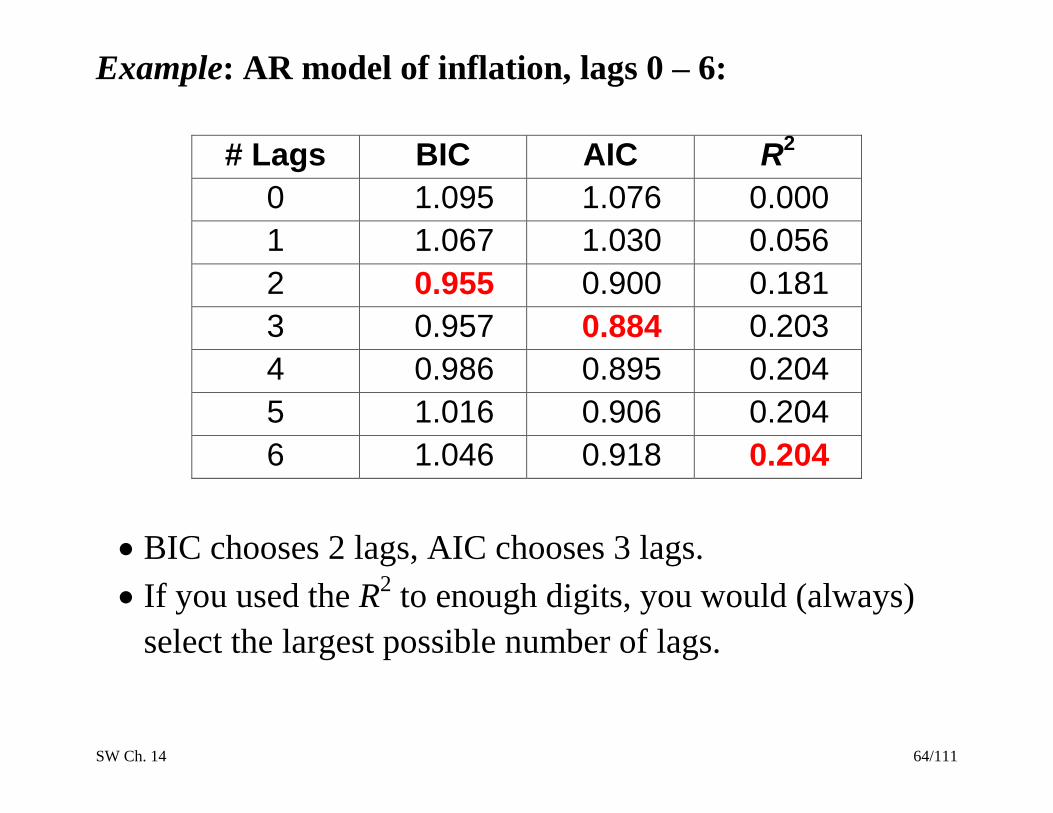
Example: AR model of inflation, lags 0 – 6:
# Lags BIC AIC R2
0 1.095 1.076 0.000
1 1.067 1.030 0.056
2 0.955 0.900 0.181
3 0.957 0.884 0.203
4 0.986 0.895 0.204
5 1.016 0.906 0.204
6 1.046 0.918 0.204
BIC chooses 2 lags, AIC chooses 3 lags.
If you used the R2 to enough digits, you would (always)
select the largest possible number of lags.
SW Ch. 14 65/111
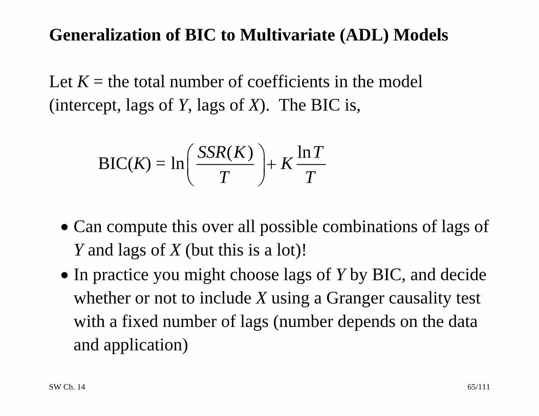
Generalization of BIC to Multivariate (ADL) Models
Let K = the total number of coefficients in the model
(intercept, lags of Y, lags of X). The BIC is,
BIC(K) = ( ) ln
lnSSR K T
KT T
Can compute this over all possible combinations of lags of
Y and lags of X (but this is a lot)!
In practice you might choose lags of Y by BIC, and decide
whether or not to include X using a Granger causality test
with a fixed number of lags (number depends on the data
and application)

SW Ch. 14 66/111
8. Nonstationarity I: Trends
(SW Section 14.6)
So far, we have assumed that the data are stationary, that is,
the distribution of (Ys+1,…, Ys+T) doesn’t depend on s.
If stationarity doesn’t hold, the series are said to be
nonstationary.
Two important types of nonstationarity are:
Trends (SW Section 14.6)
Structural breaks (model instability) (SW Section 14.7)
SW Ch. 14 67/111
Outline of discussion of trends in time series data:
A. What is a trend?
B. Deterministic and stochastic (random) trends
C. What problems are caused by trends?
D. How do you detect stochastic trends (statistical tests)?
E. How to address/mitigate problems raised by trends

SW Ch. 14 68/111
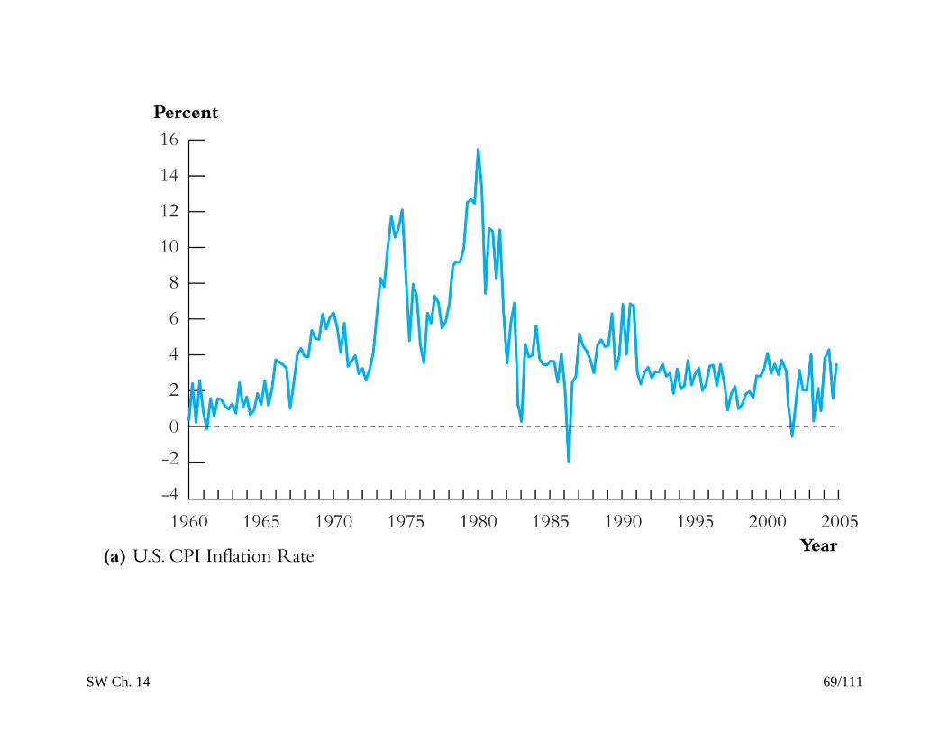
A. What is a trend?
A trend is a persistent, long-term movement or tendency in
the data. Trends need not be just a straight line!
Which of these series has a trend?
SW Ch. 14 69/111

SW Ch. 14 70/111
SW Ch. 14 71/111
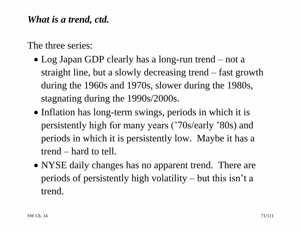
What is a trend, ctd.
The three series:
Log Japan GDP clearly has a long-run trend – not a
straight line, but a slowly decreasing trend – fast growth
during the 1960s and 1970s, slower during the 1980s,
stagnating during the 1990s/2000s.
Inflation has long-term swings, periods in which it is
persistently high for many years (’70s/early ’80s) and
periods in which it is persistently low. Maybe it has a
trend – hard to tell.
NYSE daily changes has no apparent trend. There are
periods of persistently high volatility – but this isn’t a
trend.

SW Ch. 14 72/111
B. Deterministic and stochastic trends
A trend is a long-term movement or tendency in the data.
A deterministic trend is a nonrandom function of time
(e.g. yt = t, or yt = t2).
A stochastic trend is random and varies over time
An important example of a stochastic trend is a random
walk:
Yt = Yt–1 + ut, where ut is serially uncorrelated
If Yt follows a random walk, then the value of Y tomorrow
is the value of Y today, plus an unpredictable disturbance.

SW Ch. 14 73/111
Four artificially generated random walks, T = 200:
How would you produce a random walk on the computer?

SW Ch. 14 74/111
Deterministic and stochastic trends, ctd.
Two key features of a random walk:
(i) YT+h|T = YT
Your best prediction of the value of Y in the future is the
value of Y today
To a first approximation, log stock prices follow a
random walk (more precisely, stock returns are
unpredictable)
(ii) Suppose Y0 = 0. Then var(Yt) = 2
ut .
This variance depends on t (increases linearly with t), so
Yt isn’t stationary (recall the definition of stationarity).
SW Ch. 14 75/111
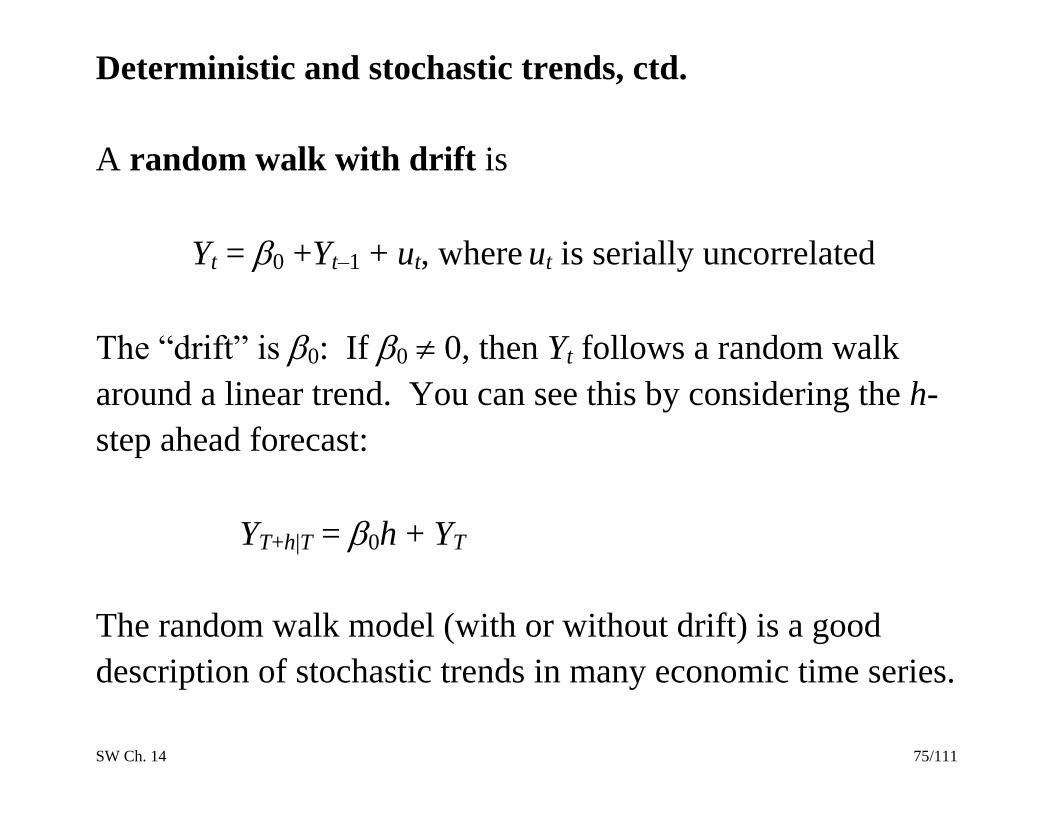
Deterministic and stochastic trends, ctd.
A random walk with drift is
Yt = 0 +Yt–1 + ut, where ut is serially uncorrelated
The “drift” is 0: If 0 0, then Yt follows a random walk
around a linear trend. You can see this by considering the h-
step ahead forecast:
YT+h|T = 0h + YT
The random walk model (with or without drift) is a good
description of stochastic trends in many economic time series.

SW Ch. 14 76/111
Deterministic and stochastic trends, ctd.
Where we are headed is the following practical advice:
If Yt has a random walk trend, then Yt is stationary
and regression analysis should be undertaken using
Yt instead of Yt.
Upcoming specifics that lead to this advice:
Relation between the random walk model and AR(1),
AR(2), AR(p) (“unit autoregressive root”)
The Dickey-Fuller test for whether a Yt has a random
walk trend

SW Ch. 14 77/111
Stochastic trends and unit autoregressive roots
Random walk (with drift): Yt = 0 + Yt–1 + ut
AR(1): Yt = 0 + 1Yt–1 + ut
The random walk is an AR(1) with 1 = 1.
The special case of 1 = 1 is called a unit root*.
When 1 = 1, the AR(1) model becomes
Yt = 0 + ut
*This terminology comes from considering the equation
1 – 1z = 0 – the “root” of this equation is z = 1/1, which equals one
(unity) if 1 = 1.
SW Ch. 14 78/111
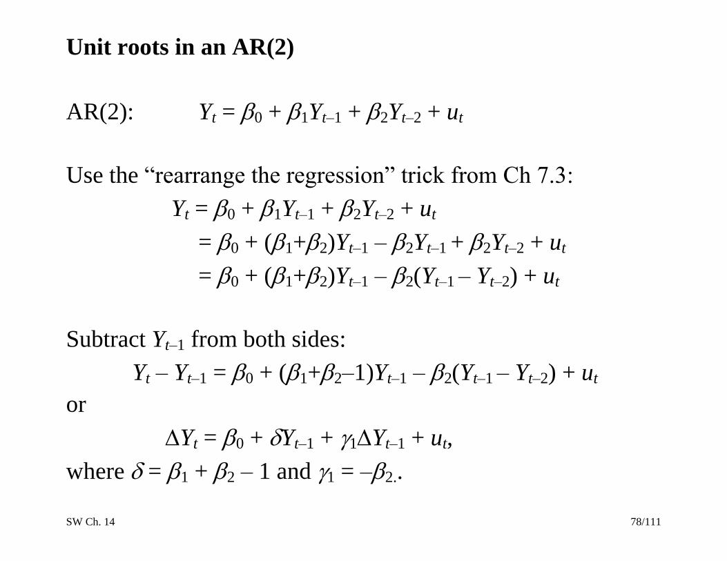
Unit roots in an AR(2)
AR(2): Yt = 0 + 1Yt–1 + 2Yt–2 + ut
Use the “rearrange the regression” trick from Ch 7.3:
Yt = 0 + 1Yt–1 + 2Yt–2 + ut
= 0 + (1+2)Yt–1 – 2Yt–1 + 2Yt–2 + ut
= 0 + (1+2)Yt–1 – 2(Yt–1 – Yt–2) + ut
Subtract Yt–1 from both sides:
Yt – Yt–1 = 0 + (1+2–1)Yt–1 – 2(Yt–1 – Yt–2) + ut
or
Yt = 0 + Yt–1 + 1Yt–1 + ut,
where = 1 + 2 – 1 and 1 = –2..

SW Ch. 14 79/111
Unit roots in an AR(2), ctd.
Thus the AR(2) model can be rearranged as,
Yt = 0 + Yt–1 + 1Yt–1 + ut
where = 1 + 2 – 1 and 1 = –2.
Claim: if 1 – 1z – 2z2 = 0 has a unit root, then 1 + 2 = 1
(show this yourself – find the roots!)
If there is a unit root, then = 0 and the AR(2) model
becomes,
Yt = 0 + 1Yt–1 + ut
If an AR(2) model has a unit root, then it can be written
as an AR(1) in first differences.
SW Ch. 14 80/111
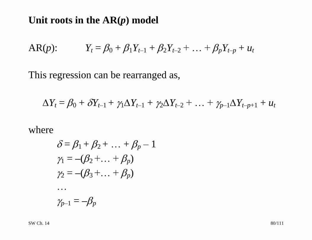
Unit roots in the AR(p) model
AR(p): Yt = 0 + 1Yt–1 + 2Yt–2 + … + pYt–p + ut
This regression can be rearranged as,
Yt = 0 + Yt–1 + 1Yt–1 + 2Yt–2 + … + p–1Yt–p+1 + ut
where
= 1 + 2 + … + p – 1
1 = –(2 +… + p)
2 = –(3 +… + p)
…
p–1 = –p
SW Ch. 14 81/111
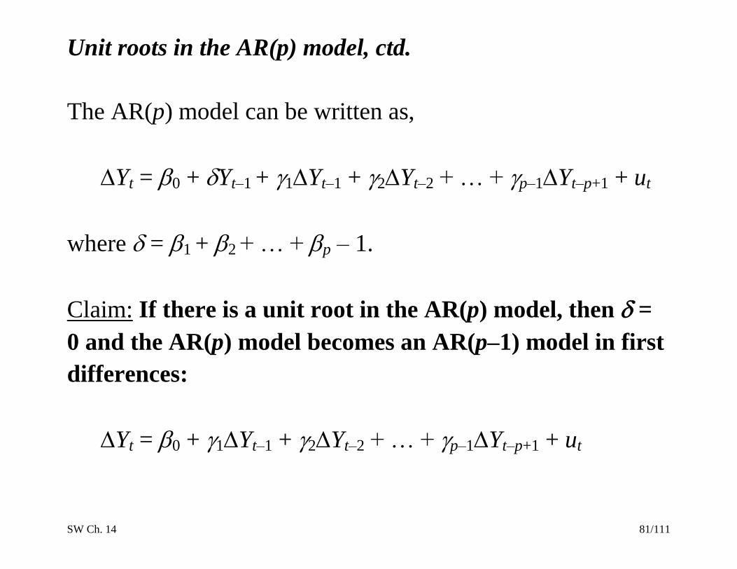
Unit roots in the AR(p) model, ctd.
The AR(p) model can be written as,
Yt = 0 + Yt–1 + 1Yt–1 + 2Yt–2 + … + p–1Yt–p+1 + ut
where = 1 + 2 + … + p – 1.
Claim: If there is a unit root in the AR(p) model, then =
0 and the AR(p) model becomes an AR(p–1) model in first
differences:
Yt = 0 + 1Yt–1 + 2Yt–2 + … + p–1Yt–p+1 + ut

SW Ch. 14 82/111
C. What problems are caused by trends?
1. AR coefficients are strongly biased towards zero. This
leads to poor forecasts.
2. Some t-statistics don’t have a standard normal
distribution, even in large samples (more on this later).
3. If Y and X both have random walk trends then they can
look related even if they are not – you can get “spurious
regressions.” Here is an example…
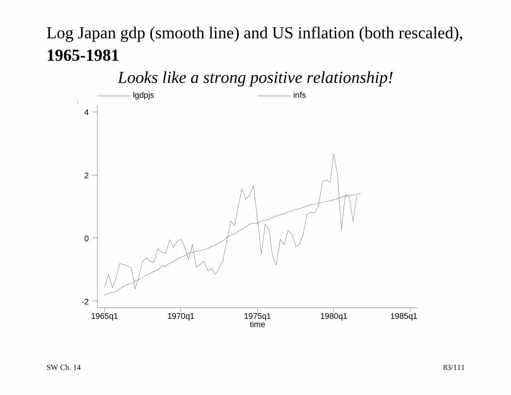
SW Ch. 14 83/111
Log Japan gdp (smooth line) and US inflation (both rescaled),
1965-1981
Looks like a strong positive relationship!
time
lgdpjs infs
1965q1 1970q1 1975q1 1980q1 1985q1
-2
0
2
4

SW Ch. 14 84/111
Log Japan gdp (smooth line) and US inflation (both rescaled),
1982-1999
What happened to that strong positive relationship?!?
time
lgdpjs infs
1980q1 1985q1 1990q1 1995q1 2000q1
-4
-2
0
2
4

SW Ch. 14 85/111
D. How do you detect stochastic trends?
1. Plot the data – are there persistent long-run movements?
2. Use a regression-based test for a random walk: the
Dickey-Fuller test for a unit root.
The Dickey-Fuller test in an AR(1)
Yt = 0 + 1Yt–1 + ut
or
Yt = 0 + Yt–1 + ut
H0: = 0 (that is, 1 = 1) v. H1: < 0
(note: this is 1-sided: < 0 means that Yt is stationary)

SW Ch. 14 86/111
DF test in AR(1), ctd.
Yt = 0 + Yt–1 + ut
H0: = 0 (that is, 1 = 1) v. H1: < 0
DF test: compute the t-statistic testing = 0
Under H0, this t statistic does not have a normal
distribution! (Our distribution theory applies to stationary
variables and Yt is nonstationary – this matters!)
You need to use the table of Dickey-Fuller critical values.
There are two cases, which have different critical values:
(a) Yt = 0 + Yt–1 + ut (intercept only)
(b) Yt = 0 + t + Yt–1 + ut (intercept & time trend)

SW Ch. 14 87/111
Table of DF Critical Values
(a) Yt = 0 + Yt–1 + ut (intercept only)
(b) Yt = 0 + t + Yt–1 + ut (intercept and time trend)
Reject if the DF t-statistic (the t-statistic testing = 0) is less
than the specified critical value. This is a 1-sided test of the
null hypothesis of a unit root (random walk trend) vs. the
alternative that the autoregression is stationary.

SW Ch. 14 88/111
The Dickey-Fuller Test in an AR(p)
In an AR(p), the DF test is based on the rewritten model,
Yt = 0 + Yt–1 + 1Yt–1 + 2Yt–2 + … + p–1Yt–p+1 + ut (*)
where = 1 + 2 + … + p – 1. If there is a unit root
(random walk trend), = 0; if the AR is stationary, < 1.
The DF test in an AR(p) (intercept only):
1. Estimate (*), obtain the t-statistic testing = 0
2. Reject the null hypothesis of a unit root if the t-statistic is
less than the DF critical value in Table 14.5
Modification for time trend: include t as a regressor in (*)

SW Ch. 14 89/111
When should you include a time trend in the DF test?
The decision to use the intercept-only DF test or the intercept
& trend DF test depends on what the alternative is – and what
the data look like.
In the intercept-only specification, the alternative is that Y
is stationary around a constant – no long-term growth in
the series
In the intercept & trend specification, the alternative is
that Y is stationary around a linear time trend – the series
has long-term growth.
SW Ch. 14 90/111
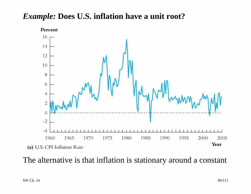
Example: Does U.S. inflation have a unit root?
The alternative is that inflation is stationary around a constant
SW Ch. 14 91/111
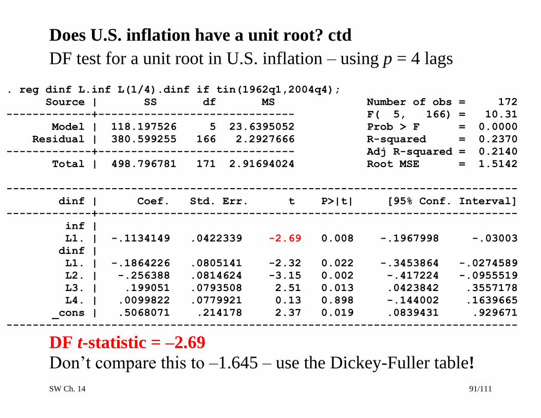
Does U.S. inflation have a unit root? ctd
DF test for a unit root in U.S. inflation – using p = 4 lags
. reg dinf L.inf L(1/4).dinf if tin(1962q1,2004q4);
Source | SS df MS Number of obs = 172
-------------+------------------------------ F( 5, 166) = 10.31
Model | 118.197526 5 23.6395052 Prob > F = 0.0000
Residual | 380.599255 166 2.2927666 R-squared = 0.2370
-------------+------------------------------ Adj R-squared = 0.2140
Total | 498.796781 171 2.91694024 Root MSE = 1.5142
------------------------------------------------------------------------------
dinf | Coef. Std. Err. t P>|t| [95% Conf. Interval]
-------------+----------------------------------------------------------------
inf |
L1. | -.1134149 .0422339 -2.69 0.008 -.1967998 -.03003
dinf |
L1. | -.1864226 .0805141 -2.32 0.022 -.3453864 -.0274589
L2. | -.256388 .0814624 -3.15 0.002 -.417224 -.0955519
L3. | .199051 .0793508 2.51 0.013 .0423842 .3557178
L4. | .0099822 .0779921 0.13 0.898 -.144002 .1639665
_cons | .5068071 .214178 2.37 0.019 .0839431 .929671
------------------------------------------------------------------------------
DF t-statistic = –2.69
Don’t compare this to –1.645 – use the Dickey-Fuller table!

SW Ch. 14 92/111
DF t-statistic = –2.69 (intercept-only):
t = –2.69 rejects a unit root at 10% level but not the 5% level
Some evidence of a unit root – not clear cut.
Whether the inflation rate has a unit root is hotly debated
among empirical monetary economists. What does it
mean for inflation to have a unit root?
We will model inflation as having a unit root.
Note: you can choose the lag length in the DF regression by
BIC or AIC (for inflation, both reject at 10%, not 5% level)

SW Ch. 14 93/111
E. How to address/mitigate problems raised by trends
If Yt has a unit root (has a random walk stochastic trend), the
easiest way to avoid the problems this poses is to model Yt in
first differences.
In the AR case, this means specifying the AR using first
differences of Yt (Yt)
This is what we did in our initial treatment of inflation –
the reason was that inspection of the plot of inflation, plus
the DF test results, suggest that inflation plausibly has a
unit root – so we estimated the ARs using Inft

SW Ch. 14 94/111
Summary: detecting and addressing stochastic trends
1. The random walk model is the workhorse model for trends
in economic time series data
2. To determine whether Yt has a stochastic trend, first plot
Yt. If a trend looks plausible, compute the DF test (decide
which version, intercept or intercept + trend)
3. If the DF test fails to reject, conclude that Yt has a unit
root (random walk stochastic trend)
4. If Yt has a unit root, use Yt for regression analysis and
forecasting. If no unit root, use Yt.

SW Ch. 14 95/111
9. Nonstationarity II: Breaks
(SW Section 14.7)
The second type of nonstationarity we consider is that the
coefficients of the model might not be constant over the full
sample. Clearly, it is a problem for forecasting if the model
describing the historical data differs from the current model –
you want the current model for your forecasts! (This is an
issue of external validity.)
So we will:
Go over two ways to detect changes in coefficients: tests
for a break, and pseudo out-of-sample forecast analysis
Work through an example: the U.S. Phillips curve

SW Ch. 14 96/111
A. Tests for a break (change) in regression coefficients
Case I: The break date is known
Suppose the break is known to have occurred at date .
Stability of the coefficients can be tested by estimating a fully
interacted regression model. In the ADL(1,1) case:
Yt = 0 + 1Yt–1 + 1Xt–1
+ 0Dt() + 1[Dt()Yt–1] + 2[Dt()Xt–1] + ut
where Dt() = 1 if t , and = 0 otherwise.
If 0 = 1 = 2 = 0, then the coefficients are constant over
the full sample.
If at least one of 0, 1, or 2 are nonzero, the regression
function changes at date .
SW Ch. 14 97/111
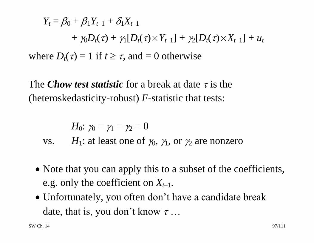
Yt = 0 + 1Yt–1 + 1Xt–1
+ 0Dt() + 1[Dt()Yt–1] + 2[Dt()Xt–1] + ut
where Dt() = 1 if t , and = 0 otherwise
The Chow test statistic for a break at date is the
(heteroskedasticity-robust) F-statistic that tests:
H0: 0 = 1 = 2 = 0
vs. H1: at least one of 0, 1, or 2 are nonzero
Note that you can apply this to a subset of the coefficients,
e.g. only the coefficient on Xt–1.
Unfortunately, you often don’t have a candidate break
date, that is, you don’t know …

SW Ch. 14 98/111
Case II: The break date is unknown
Why consider this case?
You might suspect there is a break, but not know when
You might want to test the null hypothesis of coefficient
stability against the general alternative that there has been
a break sometime.
Even if you think you know the break date, if that
“knowledge” is based on prior inspection of the series
then you have in effect “estimated” the break date. This
invalidates the Chow test critical values (why?)

SW Ch. 14 99/111
The Quandt Likelihood Ratio (QLR) Statistic
(also called the “sup-Wald” statistic)
The QLR statistic = the maximum Chow statistic
Let F() = the Chow test statistic testing the hypothesis of
no break at date .
The QLR test statistic is the maximum of all the Chow F-
statistics, over a range of , 0 1:
QLR = max[F(0), F(0+1) ,…, F(1–1), F(1)]
A conventional choice for 0 and 1 are the inner 70% of
the sample (exclude the first and last 15%).
Should you use the usual Fq, critical values?
SW Ch. 14 100/111
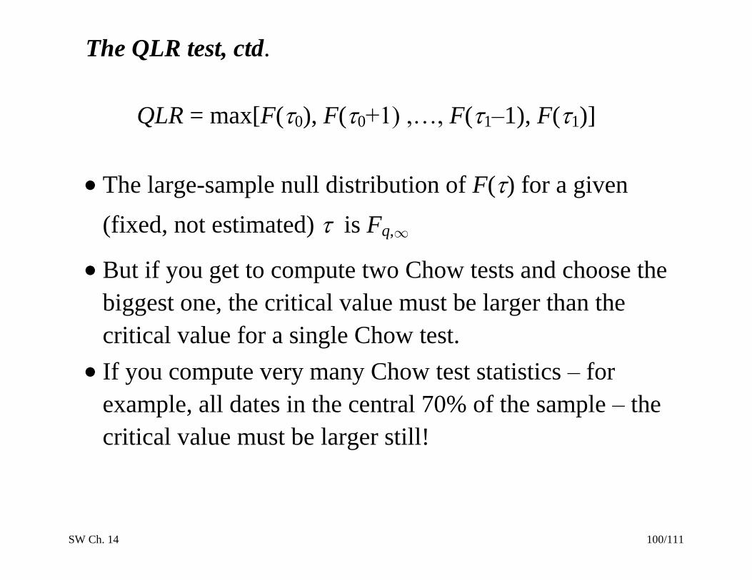
The QLR test, ctd.
QLR = max[F(0), F(0+1) ,…, F(1–1), F(1)]
The large-sample null distribution of F() for a given
(fixed, not estimated) is Fq,
But if you get to compute two Chow tests and choose the
biggest one, the critical value must be larger than the
critical value for a single Chow test.
If you compute very many Chow test statistics – for
example, all dates in the central 70% of the sample – the
critical value must be larger still!

SW Ch. 14 101/111
Get this: in large samples, QLR has the distribution,
2
1
1
1 ( )max
(1 )
q
ia s a
i
B s
q s s
,
where {Bi}, i =1,…,n, are independent continuous-time
“Brownian Bridges” on 0 ≤ s ≤ 1 (a Brownian Bridge is a
Brownian motion deviated from its mean; a Brownian
motion is a Gaussian [normally-distributed] random walk
in continuous time), and where a = .15 (exclude first and
last 15% of the sample)
Critical values are tabulated in SW Table 14.6…
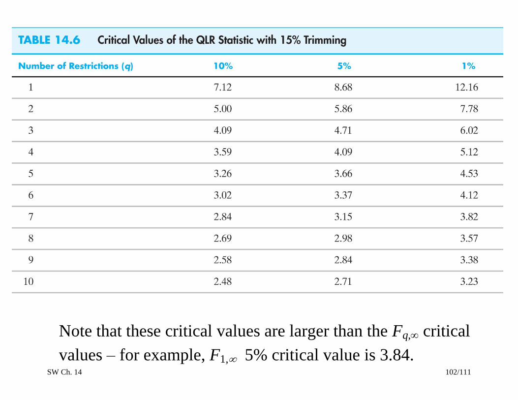
SW Ch. 14 102/111
Note that these critical values are larger than the Fq, critical
values – for example, F1, 5% critical value is 3.84.
SW Ch. 14 103/111
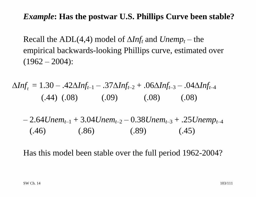
Example: Has the postwar U.S. Phillips Curve been stable?
Recall the ADL(4,4) model of Inft and Unempt – the
empirical backwards-looking Phillips curve, estimated over
(1962 – 2004):
tInf = 1.30 – .42Inft–1 – .37Inft–2 + .06Inft–3 – .04Inft–4
(.44) (.08) (.09) (.08) (.08)
– 2.64Unemt–1 + 3.04Unemt–2 – 0.38Unemt–3 + .25Unempt–4
(.46) (.86) (.89) (.45)
Has this model been stable over the full period 1962-2004?
SW Ch. 14 104/111
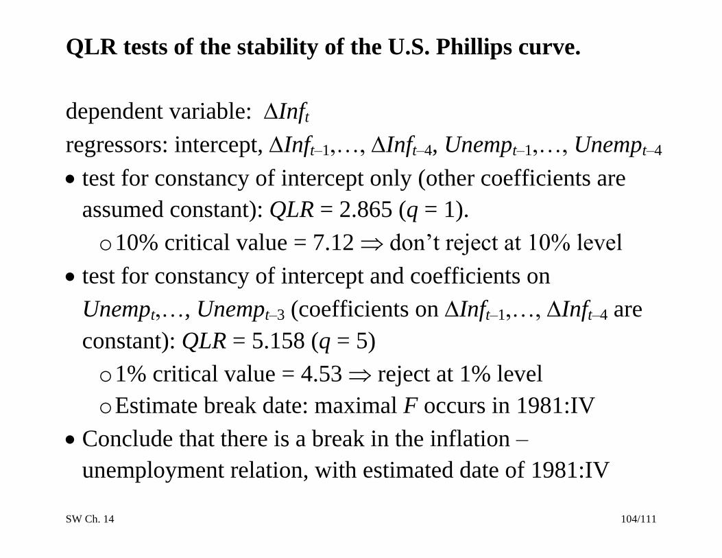
QLR tests of the stability of the U.S. Phillips curve.
dependent variable: Inft
regressors: intercept, Inft–1,…, Inft–4, Unempt–1,…, Unempt–4
test for constancy of intercept only (other coefficients are
assumed constant): QLR = 2.865 (q = 1).
o 10% critical value = 7.12 don’t reject at 10% level
test for constancy of intercept and coefficients on
Unempt,…, Unempt–3 (coefficients on Inft–1,…, Inft–4 are
constant): QLR = 5.158 (q = 5)
o 1% critical value = 4.53 reject at 1% level
o Estimate break date: maximal F occurs in 1981:IV
Conclude that there is a break in the inflation –
unemployment relation, with estimated date of 1981:IV

SW Ch. 14 105/111

SW Ch. 14 106/111
B. Assessing Model Stability using Pseudo Out-of-Sample
Forecasts
The QLR test does not work well towards the very end of
the sample – but this is usually the most interesting part!
One way to check whether the model is working at the end
of the sample is to see whether the pseudo out-of-sample
(poos) forecasts are “on track” in the most recent
observations. This is an informal diagnostic (not a formal
test) which complements formal testing using the QLR.

SW Ch. 14 107/111
Application to the U.S. Phillips Curve:
Was the U.S. Phillips Curve stable toward the end of the
sample?
We found a break in 1981:IV – so for this analysis, we only
consider regressions that start in 1982:I – ignore the earlier
data from the “old” model (“regime”).
Regression model:
dependent variable: Inft
regressors: 1, Inft–1,…, Inft–4, Unempt–1,…, Unempt–4
Pseudo out-of-sample forecasts:
o Compute regression over t = 1982:I,…, P
o Compute poos forecast, 1|P PInf , and forecast error
o Repeat for P = 1994:I,…, 2005:I

SW Ch. 14 108/111
POOS forecasts of Inf using ADL(4,4) model with Unemp
There are some big forecast errors (in 2001) but they do not
appear to be getting bigger – the model isn’t deteriorating
SW Ch. 14 109/111
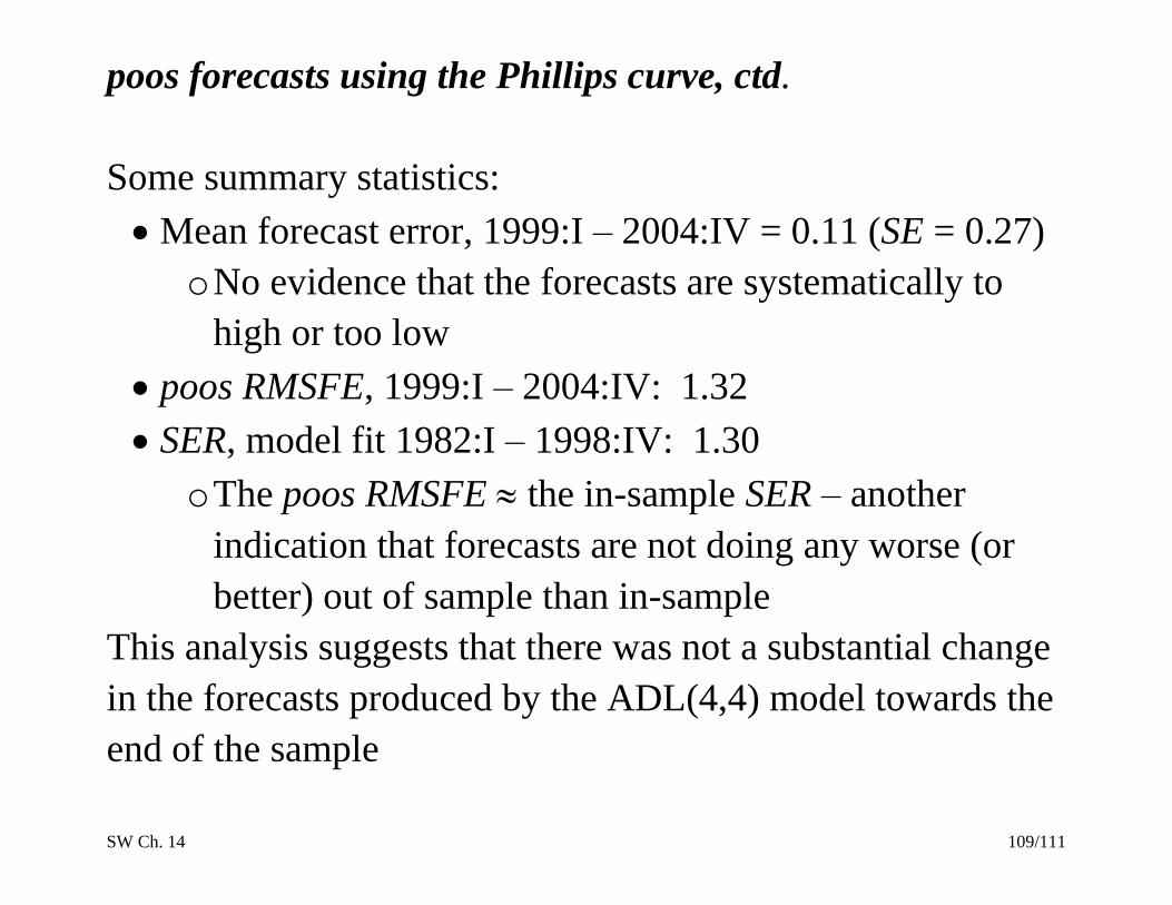
poos forecasts using the Phillips curve, ctd.
Some summary statistics:
Mean forecast error, 1999:I – 2004:IV = 0.11 (SE = 0.27)
o No evidence that the forecasts are systematically to
high or too low
poos RMSFE, 1999:I – 2004:IV: 1.32
SER, model fit 1982:I – 1998:IV: 1.30
o The poos RMSFE the in-sample SER – another
indication that forecasts are not doing any worse (or
better) out of sample than in-sample
This analysis suggests that there was not a substantial change
in the forecasts produced by the ADL(4,4) model towards the
end of the sample

SW Ch. 14 110/111
10. Conclusion: Time Series Forecasting Models
(SW Section 14.8)
For forecasting purposes, it isn’t important to have
coefficients with a causal interpretation!
The tools of regression can be used to construct reliable
forecasting models – even though there is no causal
interpretation of the coefficients:
o AR(p) – common “benchmark” models
o ADL(p,q) – add q lags of X (another predictor)
o Granger causality tests – test whether a variable X and
its lags are useful for predicting Y given lags of Y.
SW Ch. 14 111/111
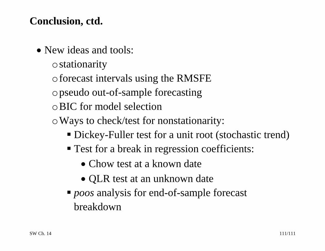
Conclusion, ctd.
New ideas and tools:
o stationarity
o forecast intervals using the RMSFE
o pseudo out-of-sample forecasting
o BIC for model selection
o Ways to check/test for nonstationarity:
Dickey-Fuller test for a unit root (stochastic trend)
Test for a break in regression coefficients:
Chow test at a known date
QLR test at an unknown date
poos analysis for end-of-sample forecast
breakdown