Introduction to the Parton Model and Pertrubative QCD

George Sterman, YITP, Stony Brook

CTEQ-Fermilab School, July 31-Aug. 9, 2012

PUCP, Lima, Peru

II. From the Parton Model to QCD

A. Color and QCD

B. Field Theory Essentials

C. Infrared Safety and Jets

1

IIA. From Color to QCD

q

q

q

?

??

?

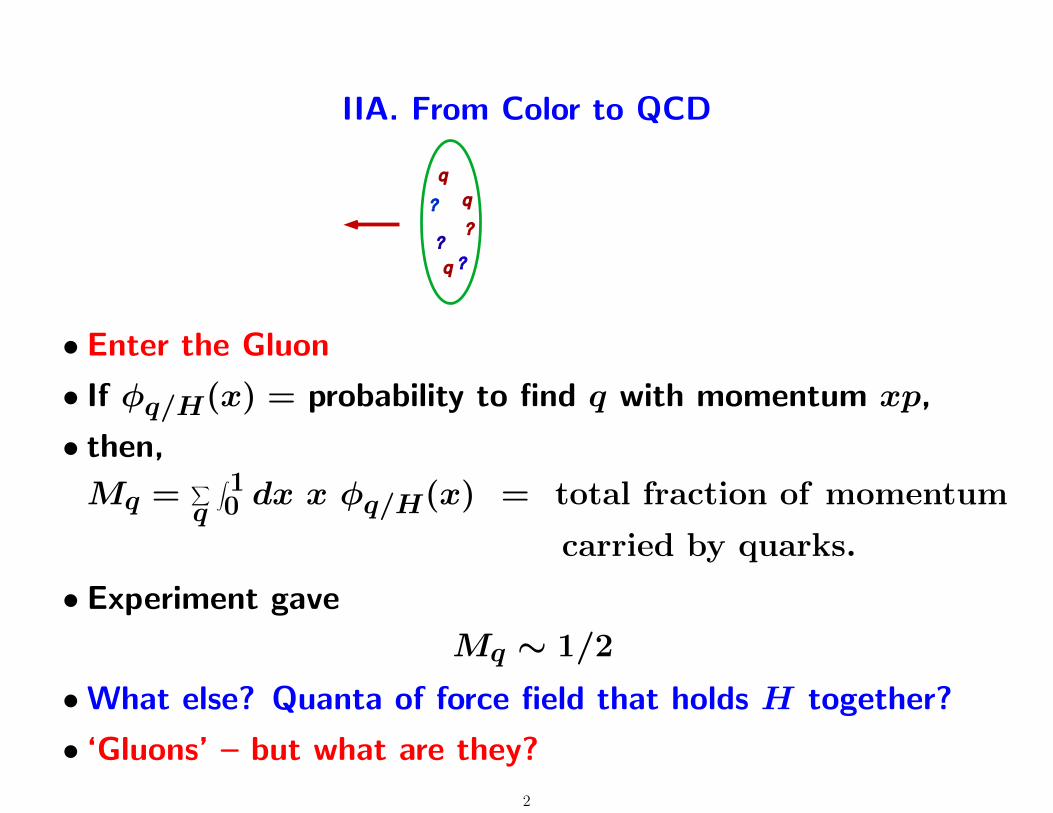
• Enter the Gluon

• If φq/H(x) = probability to find q with momentum xp,

• then,

Mq =∑

q

∫ 10 dx x φq/H(x) = total fraction of momentum

carried by quarks.

• Experiment gave

Mq ∼ 1/2

• What else? Quanta of force field that holds H together?

• ‘Gluons’ – but what are they?

2

• Where color comes from.

• Quark model problem:

– sq = 1/2⇒ fermion ⇒ antisymmetric wave function, but

– (uud) state symmetric in spin/isospin combination for nu-cleons and

– Expect the lowest-lying ψ(~xm, ~xu, ~xd) to be symmetric

– So where is the antisymmetry?

• Solution: Han Nambu, Greenberg, 1968: Color

• b, g, r, a new quantum number.

• Here’s the antisymmetry: εijkψ(~xu, ~xu, ~xd), (i,j,k)= (b,g,r)

3

• Quantum Chromodynamics: Dynamics of Color

• A globe with no north pole

Gr

b

g

gb

• Position on ‘hyperglobe’ ↔ phase of wave function(Yang & Mills, 1954)

• We can change the globe’s axes at different points in space-time, and ‘local rotation’ ↔ emission of a gluon.

• QCD: gluons coupled to the color of quarks(Gross & Wilczek; Weinberg; Fritzsch, Gell-Mann, Leutwyler, 1973)

4

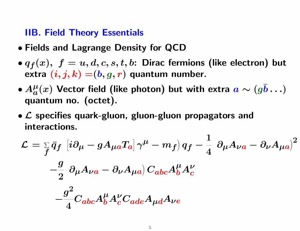
IIB. Field Theory Essentials

• Fields and Lagrange Density for QCD

• qf(x), f = u, d, c, s, t, b: Dirac fermions (like electron) butextra (i, j, k) =(b, g, r) quantum number.

•Aµa(x) Vector field (like photon) but with extra a ∼ (gb . . .)quantum no. (octet).

•L specifies quark-gluon, gluon-gluon propagators andinteractions.

L =∑

fqf

([

i∂µ − gAµaTa]

γµ −mf

)

qf −1

4

(

∂µAνa − ∂νAµa)2

−g

2

(

∂µAνa − ∂νAµa)

CabcAµbA

νc

−g2

4CabcA

µbA

νcCadeAµdAνe

5

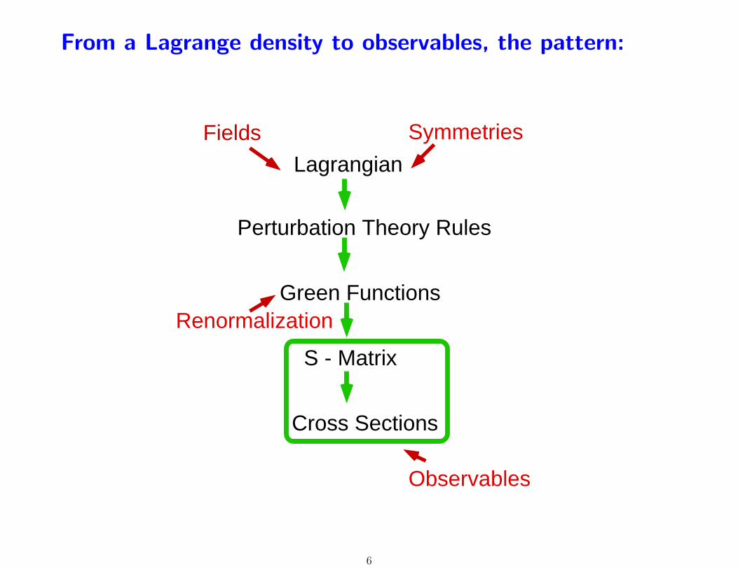
From a Lagrange density to observables, the pattern:

Lagrangian

Fields Symmetries

Perturbation Theory Rules

Green Functions

S - Matrix

Cross Sections

Observables

Renormalization

6

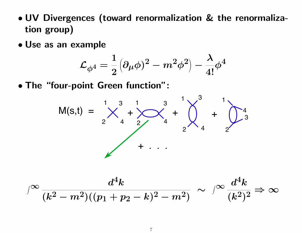
• UV Divergences (toward renormalization & the renormaliza-tion group)

• Use as an example

Lφ4 =1

2

∂µφ)2 −m2φ2

−

λ

4!φ4

• The “four-point Green function”:

M(s,t) =1

2

3

4

11 1

22 2

3

33

44

4+ ++

+ . . .

∫∞ d4k

(k2 −m2)((p1 + p2 − k)2 −m2)∼

∫∞ d4k

(k2)2⇒∞

7

Interpretation: The UV divergence is due entirely states ofhigh ‘energy deficit’,

Ein − Estate S = p01 + p0

2 −∑

i ∈S

√√√√~k2i −m2

Made explicit in Time-ordered Perturbation Theory:

1

2

3

4

=

1

2

3

4

1

2

3

4

+

E EE E

1inin 1E

out

Eout

∫ ∞ d4k

(k2 −m2)((p1 + p2 − k)2 −m2)=

∑

states

1

Ein − E1

+1

Ein − E′1

Analogy to uncertainty principle ∆E →∞⇔ ∆t→ 0.

8

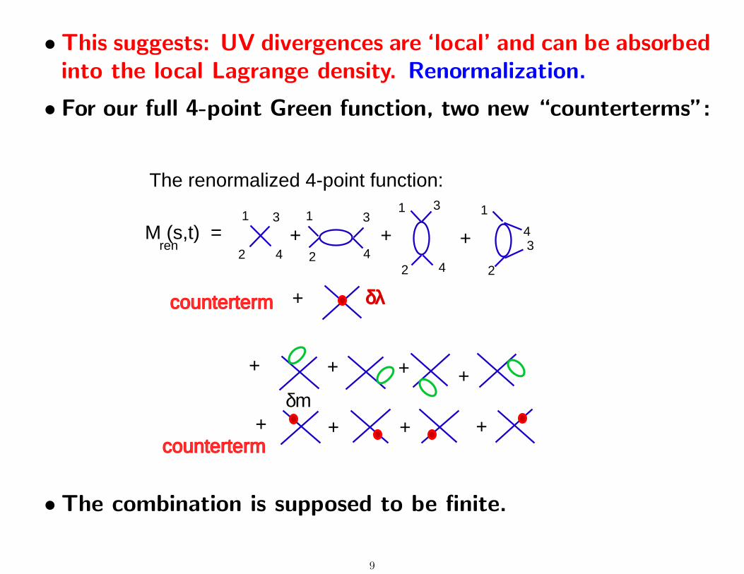
• This suggests: UV divergences are ‘local’ and can be absorbedinto the local Lagrange density. Renormalization.

• For our full 4-point Green function, two new “counterterms”:

M (s,t) =ren

1

2

3

4

1

2

3

4

1 1

2 2

3

3

4

4+ ++

+ + ++

+ + ++

+ δλ

δm

counterterm

counterterm

The renormalized 4-point function:

• The combination is supposed to be finite.

9

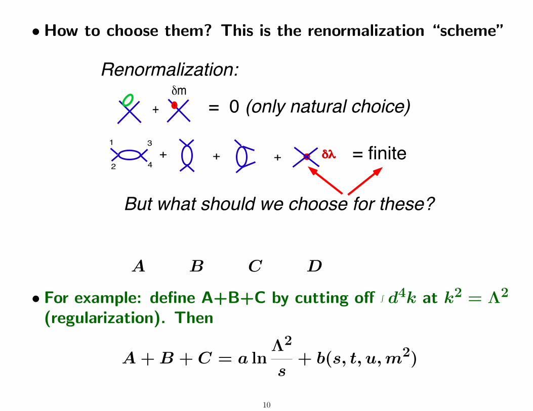
• How to choose them? This is the renormalization “scheme”

1

2

3

4

++ + !" = finite

+

!m

= 0 (only natural choice)

{{{

Renormalization:

But what should we choose for these?

A B C D

• For example: define A+B+C by cutting off ∫ d4k at k2 = Λ2

(regularization). Then

A+B + C = a lnΛ2

s+ b(s, t, u,m2)

10

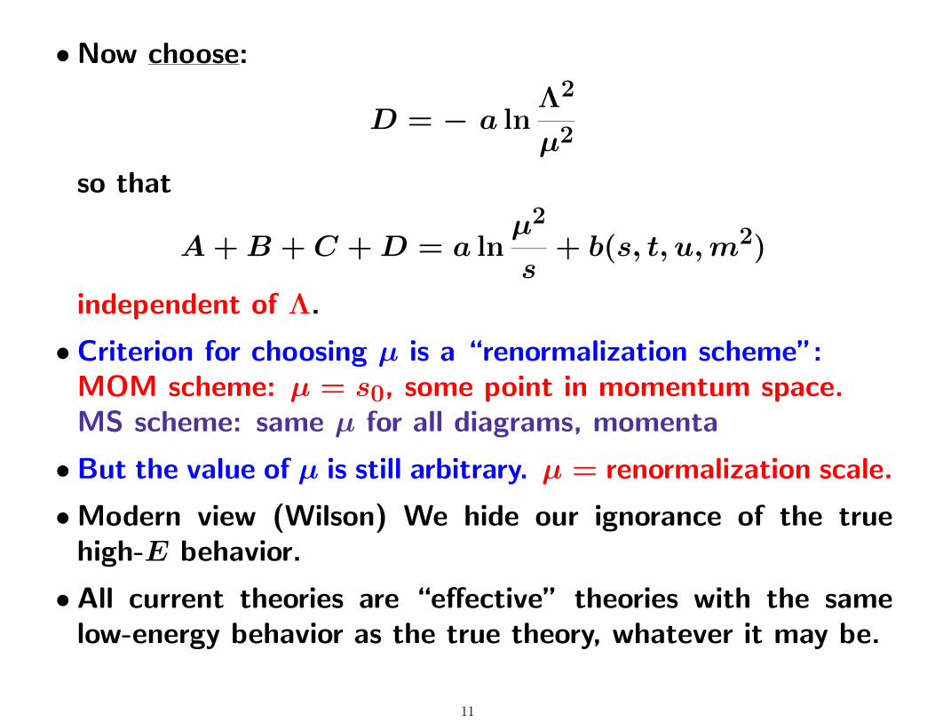
• Now choose:

D = − a lnΛ2

µ2

so that

A+B + C +D = a lnµ2

s+ b(s, t, u,m2)

independent of Λ.

• Criterion for choosing µ is a “renormalization scheme”:MOM scheme: µ = s0, some point in momentum space.MS scheme: same µ for all diagrams, momenta

• But the value of µ is still arbitrary. µ = renormalization scale.

• Modern view (Wilson) We hide our ignorance of the truehigh-E behavior.

• All current theories are “effective” theories with the samelow-energy behavior as the true theory, whatever it may be.

11

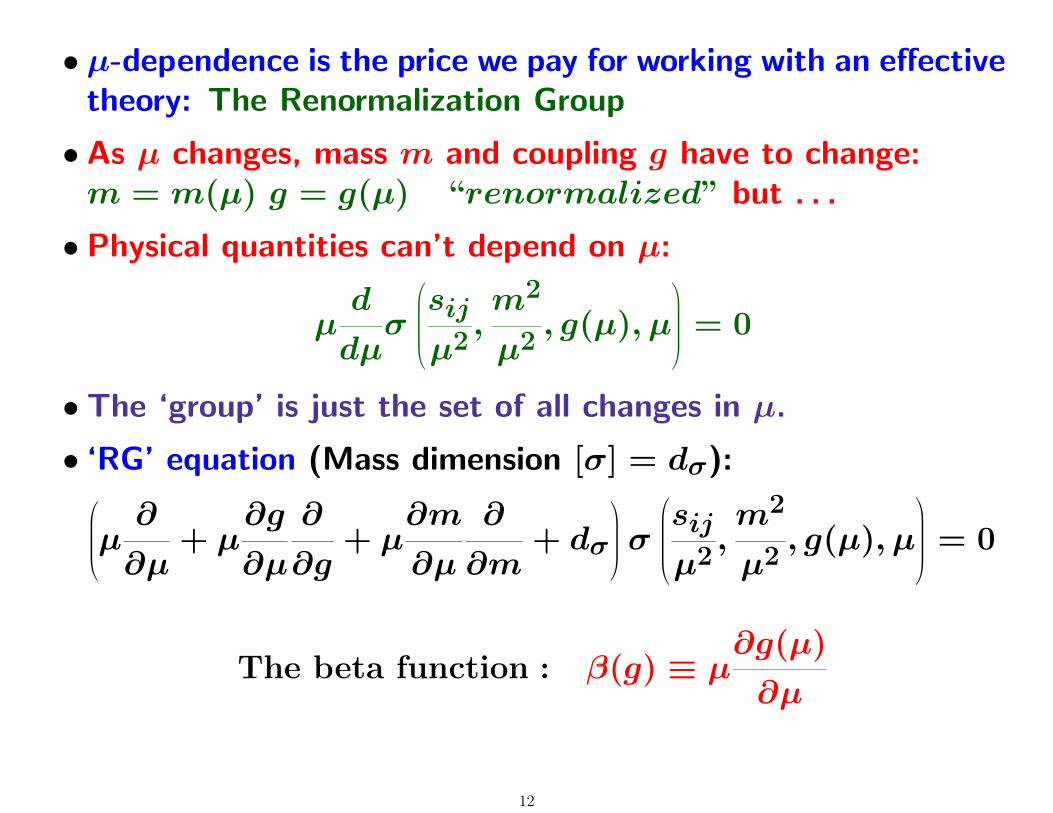
• µ-dependence is the price we pay for working with an effectivetheory: The Renormalization Group

• As µ changes, mass m and coupling g have to change:m = m(µ) g = g(µ) “renormalized” but . . .

• Physical quantities can’t depend on µ:

µd

dµσ

sij

µ2,m2

µ2, g(µ), µ

= 0

• The ‘group’ is just the set of all changes in µ.

• ‘RG’ equation (Mass dimension [σ] = dσ):µ∂

∂µ+ µ

∂g

∂µ

∂

∂g+ µ

∂m

∂µ

∂

∂m+ dσ

σ

sij

µ2,m2

µ2, g(µ), µ

= 0

The beta function : β(g) ≡ µ∂g(µ)

∂µ

12

• The Running coupling

• Consider any σ (m = 0, dσ = 0) with kinematic invariantssij = (pi + pj)

2:

µdσ

dµ= 0 → µ

∂σ

∂µ= −β(g)

∂σ

∂g(1)

• in PT:

σ = g2(µ)σ(1) + g4(µ)

σ

(2)

sij

skl

+ τ (2) ln

s12

µ2

+ . . . (2)

• (2) in (1) →g4τ (2) = 2gσ(1)β(g) + . . .

β(g) =g3

2

τ (2)

σ(1)+O(g5) ≡ −

g3

16π2β0 +O(g5)

• In QCD:

β0 = 11−2nf

3•−β0 < 0 → g decreases as µ increases.

13

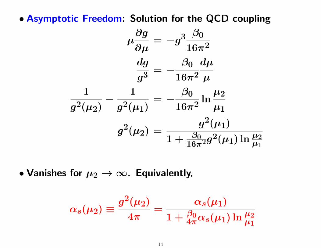
• Asymptotic Freedom: Solution for the QCD coupling

µ∂g

∂µ= −g3 β0

16π2

dg

g3= −

β0

16π2

dµ

µ

1

g2(µ2)−

1

g2(µ1)= −

β0

16π2lnµ2

µ1

g2(µ2) =g2(µ1)

1 + β016π2g

2(µ1) ln µ2µ1

• Vanishes for µ2→∞. Equivalently,

αs(µ2) ≡g2(µ2)

4π=

αs(µ1)

1 + β04παs(µ1) ln µ2

µ1

14

• Dimensional transmutation: ΛQCD

– Two mass scales appear in

αs(µ2) =αs(µ1)

1 + β04παs(µ1) ln µ2

µ1

but the value of αs(µ2) can’t depend on choice of µ1.

– Reduce it to one by defining Λ ≡ µ1 e−β0/αs(µ1), indepen-

dent of µ1. Then

αs(µ2) =4π

β0 ln µ22

Λ2

• Asymptotic freedom strongly suggests a relationship to theparton model, in which partons act as if free at short dis-tances. But how to quantify this observation?

15

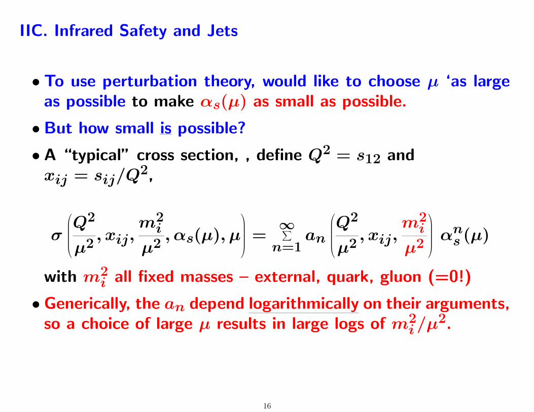
IIC. Infrared Safety and Jets

• To use perturbation theory, would like to choose µ ‘as largeas possible to make αs(µ) as small as possible.

• But how small is possible?

• A “typical” cross section, , define Q2 = s12 andxij = sij/Q

2,

σ

Q2

µ2, xij,

m2i

µ2, αs(µ), µ

=∞∑n=1

an

Q2

µ2, xij,

m2i

µ2

αns (µ)

with m2i all fixed masses – external, quark, gluon (=0!)

• Generically, the an depend logarithmically on their arguments,so a choice of large µ results in large logs of m2

i/µ2.

16

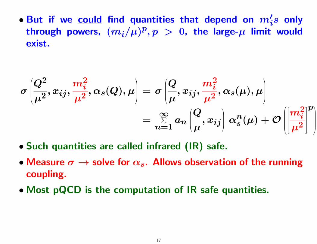
• But if we could find quantities that depend on m′is onlythrough powers, (mi/µ)p, p > 0, the large-µ limit wouldexist.

σ

Q2

µ2, xij,

m2i

µ2, αs(Q), µ

= σ

Q

µ, xij,

m2i

µ2, αs(µ), µ

=∞∑n=1

an

Q

µ, xij

α

ns (µ) +O

m2i

µ2

p

• Such quantities are called infrared (IR) safe.

• Measure σ → solve for αs. Allows observation of the runningcoupling.

• Most pQCD is the computation of IR safe quantities.

17

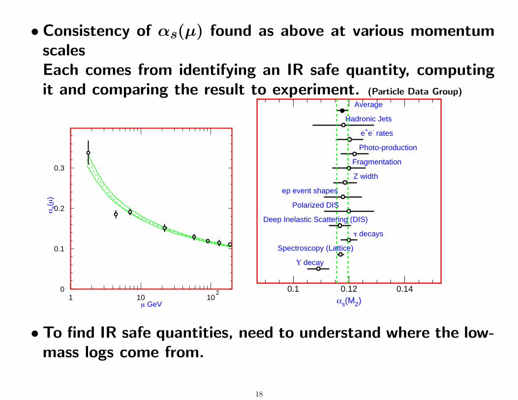
• Consistency of αs(µ) found as above at various momentumscalesEach comes from identifying an IR safe quantity, computingit and comparing the result to experiment. (Particle Data Group)

0

0.1

0.2

0.3

1 10 102

µ GeV

αs(µ

)

0.1 0.12 0.14

Average

Hadronic Jets

Polarized DIS

Deep Inelastic Scattering (DIS)

τ decays

Z width

Fragmentation

Spectroscopy (Lattice)

ep event shapes

Photo-production

Υ decay

e+e- rates

αs(MZ)

• To find IR safe quantities, need to understand where the low-mass logs come from.

18

• To analyze diagrams, we generally think of m → 0 limit inm/Q. Gives “IR” logs.

• Generic source of IR (soft and collinear) logarithms:

p

αp

• IR logs come from degenerate states:Uncertainty principle ∆E → 0⇔ ∆t→∞.

• For soft emission and collinear splitting it’s “never too late”.But these processes don’t change the flow of energy . . .Problems arise if we ask for particle content.

19

• For IR safety, sum over degenerate final states in perturbationtheory, and don’t ask how many particles of each kind we have.This requires us to introduce another regularization, this timefor IR behavior.

• The IR regulated theory is like QCD at short distances, butis better-behaved at long distances.

• IR-regulated QCD not the same as QCD except for IR safequantities.

20

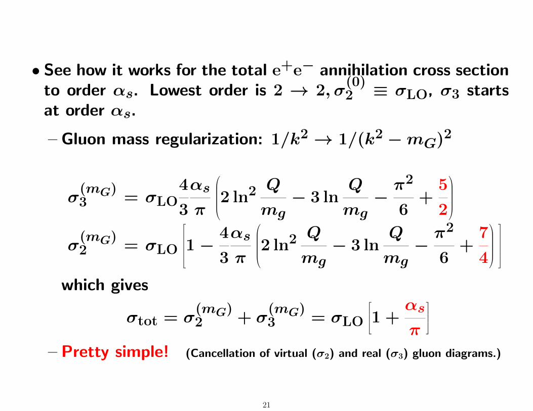
• See how it works for the total e+e− annihilation cross sectionto order αs. Lowest order is 2 → 2, σ

(0)2 ≡ σLO, σ3 starts

at order αs.

– Gluon mass regularization: 1/k2→ 1/(k2 −mG)2

σ(mG)3 = σLO

4

3

αs

π

2 ln2 Q

mg− 3 ln

Q

mg−π2

6+

5

2

σ(mG)2 = σLO

1−

4

3

αs

π

2 ln2 Q

mg− 3 ln

Q

mg−π2

6+

7

4

which gives

σtot = σ(mG)2 + σ

(mG)3 = σLO

1 +

αs

π

– Pretty simple! (Cancellation of virtual (σ2) and real (σ3) gluon diagrams.)

21

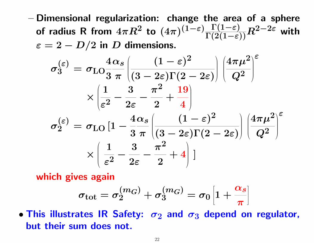
– Dimensional regularization: change the area of a sphere

of radius R from 4πR2 to (4π)(1−ε) Γ(1−ε)Γ(2(1−ε))R

2−2ε with

ε = 2−D/2 in D dimensions.

σ(ε)3 = σLO

4

3

αs

π

(1− ε)2

(3− 2ε)Γ(2− 2ε)

4πµ2

Q2

ε

×

1

ε2−

3

2ε−π2

2+

19

4

σ(ε)2 = σLO [1−

4

3

αs

π

(1− ε)2

(3− 2ε)Γ(2− 2ε)

4πµ2

Q2

ε

×

1

ε2−

3

2ε−π2

2+ 4

]

which gives again

σtot = σ(mG)2 + σ

(mG)3 = σ0

1 +

αs

π

• This illustrates IR Safety: σ2 and σ3 depend on regulator,but their sum does not.

22

• Generalized IR safety: sum over all states with the sameflow of energy into the final state. Introduce IR safe weight“e({pi})”

dσ

de=

∑

n

∫

PS(n) |M({pi})|2δ (e({pi})− w)

with

e(. . . pi . . . pj−1, αpi, pj+1 . . .) =

e(. . . (1 + α)pi . . . pj−1, pj+1 . . .)

• Neglect long times in the initial state for the moment andsee how this works in e+e− annihilation: event shapes andjet cross sections.

23

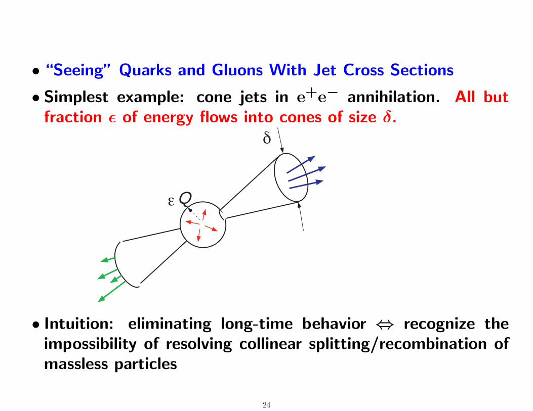
• “Seeing” Quarks and Gluons With Jet Cross Sections

• Simplest example: cone jets in e+e− annihilation. All butfraction ε of energy flows into cones of size δ.

!

"Q

• Intuition: eliminating long-time behavior ⇔ recognize theimpossibility of resolving collinear splitting/recombination ofmassless particles

24

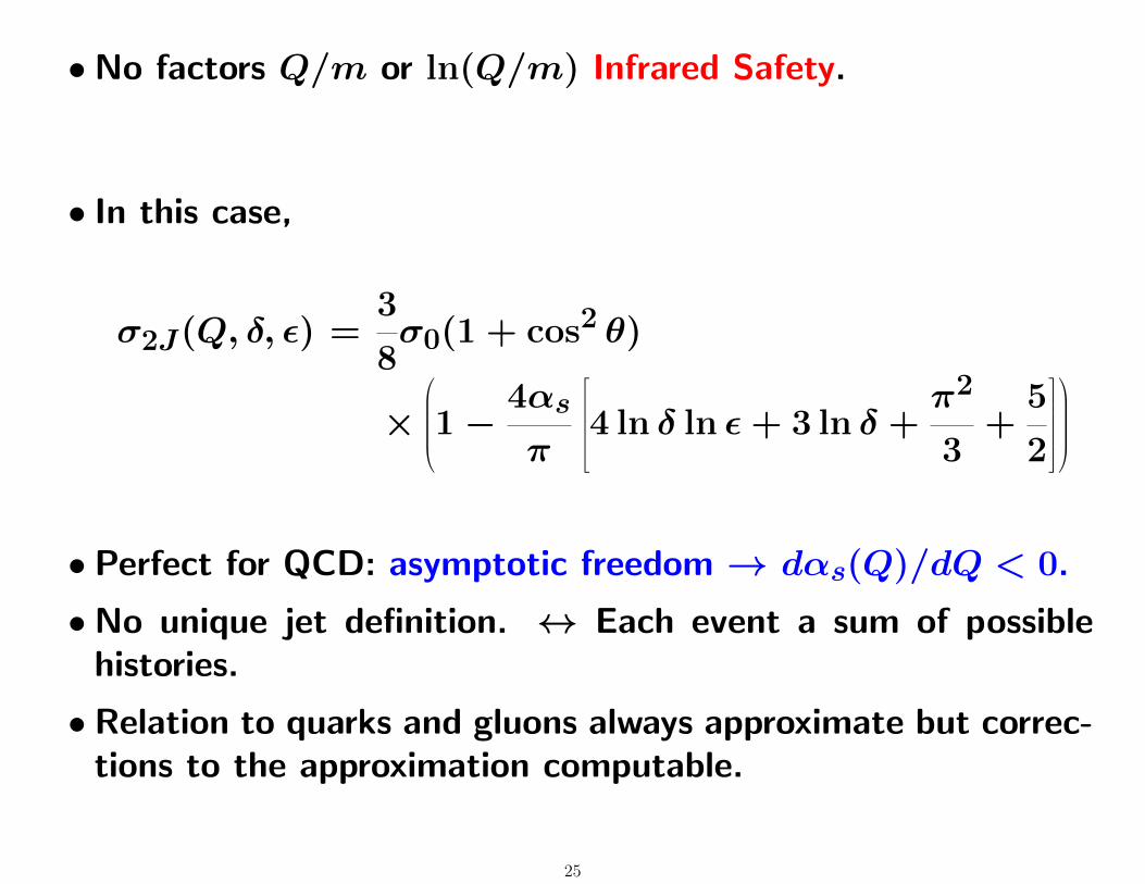
• No factors Q/m or ln(Q/m) Infrared Safety.

• In this case,

σ2J(Q, δ, ε) =3

8σ0(1 + cos2 θ)

×1−

4αs

π

4 ln δ ln ε+ 3 ln δ +

π2

3+

5

2

• Perfect for QCD: asymptotic freedom → dαs(Q)/dQ < 0.

• No unique jet definition. ↔ Each event a sum of possiblehistories.

• Relation to quarks and gluons always approximate but correc-tions to the approximation computable.

25

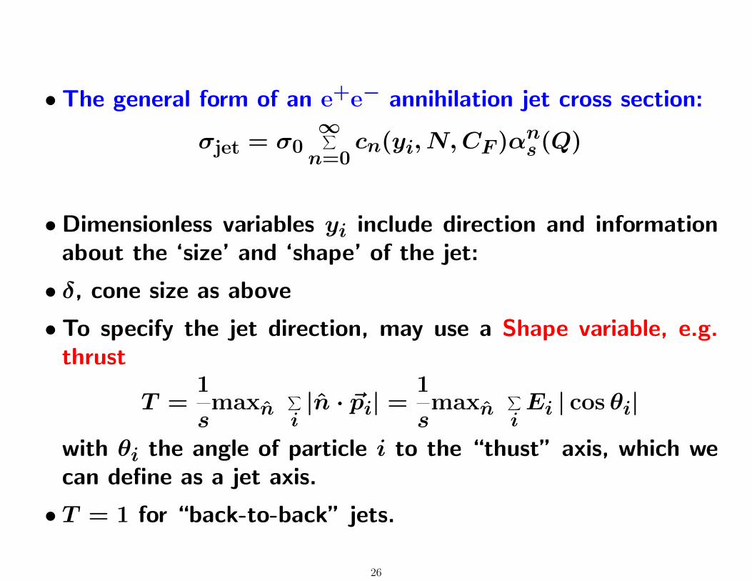
• The general form of an e+e− annihilation jet cross section:

σjet = σ0∞∑n=0

cn(yi, N,CF )αns (Q)

• Dimensionless variables yi include direction and informationabout the ‘size’ and ‘shape’ of the jet:

• δ, cone size as above

• To specify the jet direction, may use a Shape variable, e.g.thrust

T =1

smaxn

∑

i|n · ~pi| =

1

smaxn

∑

iEi | cos θi|

with θi the angle of particle i to the “thust” axis, which wecan define as a jet axis.

• T = 1 for “back-to-back” jets.

26

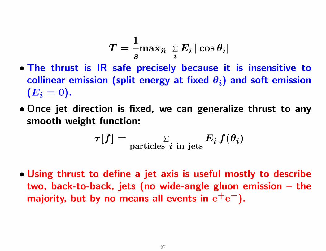
T =1

smaxn

∑

iEi | cos θi|

• The thrust is IR safe precisely because it is insensitive tocollinear emission (split energy at fixed θi) and soft emission(Ei = 0).

• Once jet direction is fixed, we can generalize thrust to anysmooth weight function:

τ [f ] =∑

particles i in jetsEi f(θi)

• Using thrust to define a jet axis is useful mostly to describetwo, back-to-back, jets (no wide-angle gluon emission – themajority, but by no means all events in e+e−).

27

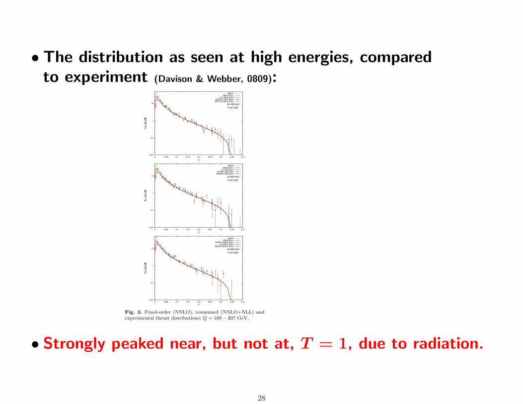
• The distribution as seen at high energies, comparedto experiment (Davison & Webber, 0809):4 R.A. Davison, B.R. Webber: Non-Perturbative Contribution to the Thrust Distribution in e+e− Annihilation

0.01

0.1

1

10

0 0.05 0.1 0.15 0.2 0.25 0.3 0.35 0.4

1/!

d!

/dt

t

Q=189 GeV

"s=0.1060

NNLONNLO+NLL

L3 (188.6 GeV)ALEPH (189.0 GeV)

DELPHI (189.0 GeV)

0.01

0.1

1

10

0 0.05 0.1 0.15 0.2 0.25 0.3 0.35 0.4

1/!

d!

/dt

t

Q=200 GeV

"s=0.1052

NNLONNLO+NLL

L3 (200 GeV)ALEPH (200 GeV)

DELPHI (200 GeV)

0.01

0.1

1

10

0 0.05 0.1 0.15 0.2 0.25 0.3 0.35 0.4

1/!

d!

/dt

t

Q=206 GeV

"s=0.1048

NNLONNLO+NLL

ALEPH (206.0 GeV)L3 (206.2 GeV)

DELPHI (207.0 GeV)

Fig. 3. Fixed-order (NNLO), resummed (NNLO+NLL) andexperimental thrust distributions: Q = 189 − 207 GeV.

where

C (αs) = 1 +

∞�

n=1

Cnαns ,

lnΣ (y,αs) =∞�

n=1

n+1�

m=1

Gnmαns Lm

= Lg1 (αsL) + g2 (αsL) + αsg3 (αsL) + . . . ,(11)

L = ln(1/y) and D (y,αs) is a remainder function thatvanishes order-by-order in perturbation theory in the two-jet limit y → 0. The functions gi (αsL) are power se-ries in αsL (with no leading constant term) and henceLg1 (αsL) sums all leading logarithms αn

s Ln+1, g2 (αsL)sums all next-to-leading logarithms (NLL) αn

s Ln and thesubdominant logarithmic terms αn

s Lm with 0 < m < nare contained in the g3, g4, . . . terms. The functions gi thusresum the logarithmic contributions at all orders in per-turbation theory, and knowledge of their form allows usto make accurate perturbative predictions in the range

αsL � 1 – a significant improvement on the fixed-orderrange αsL

2 � 1.For thrust, the first two functions can be determined

analytically by using the coherent branching formalism [11,12], which uses consecutive branchings from an initial quark-antiquark state to produce multi-parton final states toNLL accuracy. The results of this calculation depend uponthe jet mass distribution J

�Q2, k2

�– the probability of

producing a final state jet with invariant mass k2 from aparent parton produced in a hard process at scale Q2 –and its Laplace transform Jν

�Q2�. To the required accu-

racy, the thrust distribution is

1

σ

dσ

dt=

Q2

2πi

�

C

dνetνQ2�Jµν

�Q2��2

, (12)

where the contour C runs parallel to the imaginary axison the right of all singularities of the integrand,

ln Jµν

�Q2�

=

� 1

0

du

u

�e−uνQ2 − 1

��� uQ2

u2Q2

dµ2

µ2CF

αs (µ)

π

�1 − K

αs (µ)

2π

�−1

+ . . .

�, (13)

and2

K = N

�67

18− π2

6

�− 5

9NF . (14)

This expression demonstrates explicitly that the diver-gence of αs (µ) at low µ will affect the perturbative thrustdistribution – such effects are related to the renormalonmentioned earlier. To NLL accuracy, however, we can ne-glect the low µ region (although we will return to it inSect. 4) to give the thrust resummation functions [10]

g1 (αsL) = 2f1 (β0αsL) ,

g2 (αsL) = 2f2 (β0αsL) − lnΓ [1 − 2f1 (β0αsL)

− 2β0αsLf �1 (β0αsL)],

(15)

where

f1 (x) = − CF

β0x[(1 − 2x) ln (1 − 2x)

− 2 (1 − x) ln (1 − x)],

f2 (x) = − CF K

β20

[2 ln (1 − x) − ln (1 − 2x)]

− 3CF

2β0ln (1 − x) − 2CF γE

β0[ln (1 − x)

− ln (1 − 2x)] − CFβ1

β30

�ln (1 − 2x)

− 2 ln (1 − x) +1

2ln2 (1 − 2x) − ln2 (1 − x)

�,

(16)

2 By writing the K dependence in the form shown in (13), wechange from the MS renormalisation scheme to the so-calledbremsstrahlung scheme [13].

• Strongly peaked near, but not at, T = 1, due to radiation.

28

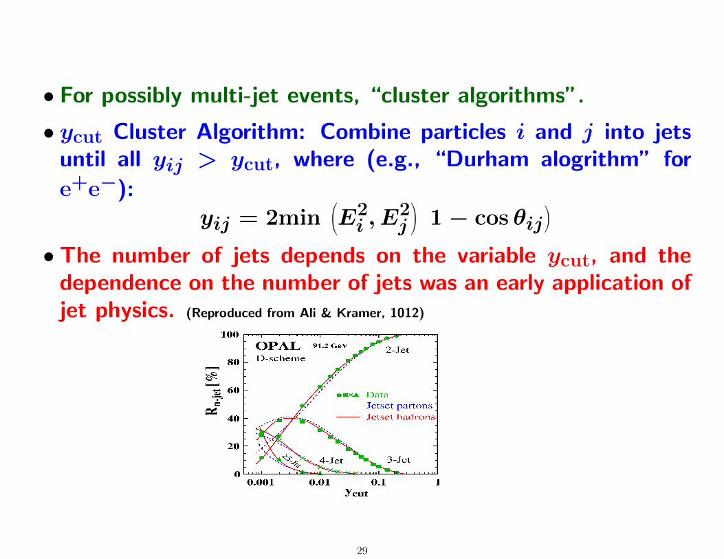
• For possibly multi-jet events, “cluster algorithms”.

• ycut Cluster Algorithm: Combine particles i and j into jetsuntil all yij > ycut, where (e.g., “Durham alogrithm” for

e+e−):yij = 2min

E2i , E

2j

(

1− cos θij)

• The number of jets depends on the variable ycut, and thedependence on the number of jets was an early application ofjet physics. (Reproduced from Ali & Kramer, 1012)

Will be inserted by the editor 41

Fig. 25. Measured distributions of thrust, T, (left-hand frame) and the C-parameter incomparison with QCD predictions at

√s =206.2 GeV [From L3 [148]].

Fig. 26. Relative production rates of n-jet events defined in the Durham jet algorithmscheme [54] as a function of the jet resolution parameter ycut. The data are comparedto model calculations before and after the hadronization process as indicated on the fig-ure [OPAL[161]].

the solid lines corresponding to a fixed value xµ = 1, and the dashed lines are theresults obtained with a fitted scale, indicated on the figure. This and related anal-yses reported in [147] yield a rather precise value for the QCD coupling constantαs(MZ) = 0.11870.0034

−0.0019. At LEP2 (up to√

s = 206 GeV), the highest jet multi-plicity measured is five, obtained using the variable ycut, and inclusive measurementsare available for up to six jets. To match this data, NLO QCD corrections to five-jetproduction at LEP have been carried out by Frederix "et al. [162], and the fixed-orderperturbative results have been compared with the LEP1 data from ALEPH [149].Two observables have been used for this comparison:

29

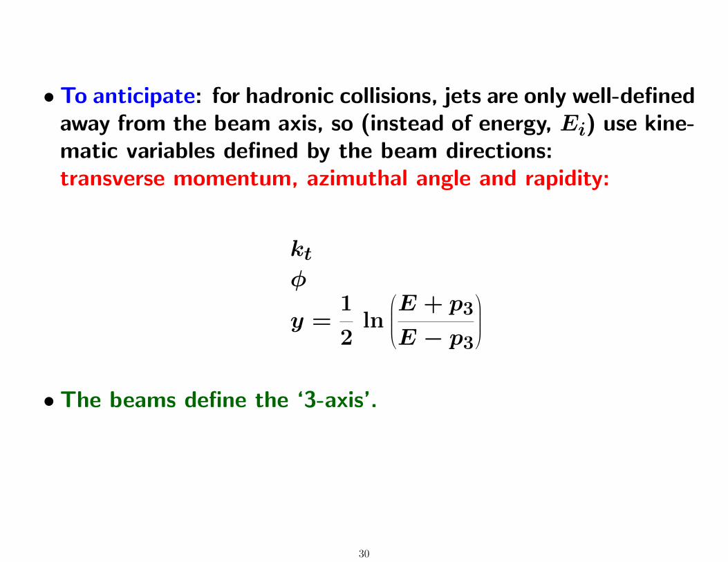
• To anticipate: for hadronic collisions, jets are only well-definedaway from the beam axis, so (instead of energy, Ei) use kine-matic variables defined by the beam directions:transverse momentum, azimuthal angle and rapidity:

ktφ

y =1

2ln

E + p3

E − p3

• The beams define the ‘3-axis’.

30

• Cluster variables for hadronic collisions:

dij = mink

2pti , k

2ptj

∆2ij

R2

∆2ij = (yi−yj)2 +(φi−φj)2. R is an adjustable parameter.

• The “classic” choices:

– p = 1 “kt algorithm:

– p = 0 “Cambridge/Aachen”

– p = −1 “anti-kt”

31

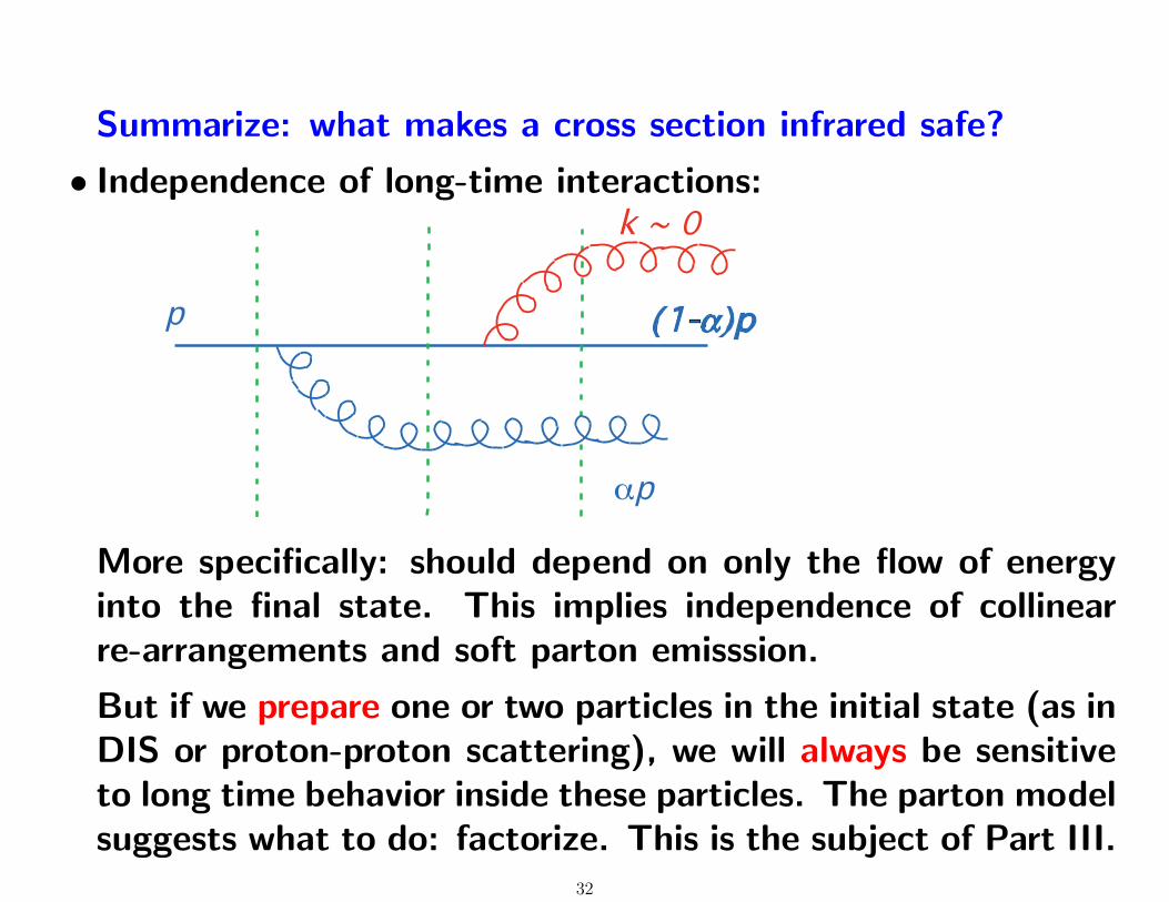
Summarize: what makes a cross section infrared safe?

• Independence of long-time interactions:

p

αp

More specifically: should depend on only the flow of energyinto the final state. This implies independence of collinearre-arrangements and soft parton emisssion.

But if we prepare one or two particles in the initial state (as inDIS or proton-proton scattering), we will always be sensitiveto long time behavior inside these particles. The parton modelsuggests what to do: factorize. This is the subject of Part III.

32