Embed Size (px)
Citation preview

GPDs, part I
QCD&Hadrons
LC formalism
FFs
PDFs
DIS
NPDs
Models
Generalized Parton DistributionsA.V. Radyushkin
Physics Department, Old Dominion University&
Theory Center, Jefferson Lab

GPDs, part I
QCD&Hadrons
LC formalism
FFs
PDFs
DIS
NPDs
Models
QCD as Fundamental Physics
Example of fundamental physics:search for Higgs boson
Motivation: HB is responsible for mass generation
Observation: By far the largest part of visible mass around usis due to nucleons, mN/me ∼ 2000
⇒ From 940 MeV of mN , only < 30 MeV (currentquark masses) may be related to Higgs particle
⇒ Most part of mass is due to gluons,which are massless!
Situation in hadronic physics:
All relevant fundamental particlesestablished
QCD Lagrangian is known
Need to understand how QCD works

GPDs, part I
QCD&Hadrons
LC formalism
FFs
PDFs
DIS
NPDs
Models
Hadrons in Terms of Quarks and Gluons
How to relate hadronic states |p, s〉to quark and gluon fields q(z1) , q(z2) , . . . ?
Standard way: use matrix elements
〈 0 | qα(z1) qβ(z2) |M(p), s 〉 , 〈 0 | qα(z1) qβ(z2) qγ(z3)|B(p), s 〉
Can be interpreted as hadronic wave functions

GPDs, part I
QCD&Hadrons
LC formalism
FFs
PDFs
DIS
NPDs
Models
Light-cone formalism
Describe hadron by Fock components ininfinite-momentum frame
For nucleon
|P 〉 = ψqqq|q(x1P, k1⊥) q(x2P, k2⊥) q(x3P, k3⊥)〉+ ψqqqG|qqqG〉+ ψqqqqq|qqqqq〉+ ψqqqGG|qqqGG〉+ . . .
xi : momentum fractions∑i
xi = 1
ki⊥: transverse momenta∑i
ki⊥ = 0

GPDs, part I
QCD&Hadrons
LC formalism
FFs
PDFs
DIS
NPDs
Models
Basics of LC Formalism
Take a fast-moving hadron with momentum p inz-direction:
pz →∞ , E =√p2z +m2 →∞ , E2−p2
z = m2 � p2z, E
2
p2 in components:
p2 = p20 − p2
z = (p0 + pz)(p0 − pz) ≡ p+p−
Note: “Plus" component p+ is large, “minus” componentp− = m2/p+ is smallMomentum p is close to a “light cone" vector P , forwhich P− is zero, and P 2 = 0
pµ = Pµ + p2nµ + 0⊥
Light-cone basis vectors:
P 2 = 0 , n2 = 0 , 2(Pn) = 1

GPDs, part I
QCD&Hadrons
LC formalism
FFs
PDFs
DIS
NPDs
Models
Two-particle system in LC Formalism
Take a qq component of a meson, with quarks havingmomenta k and p− k:
k =xP + yn+ k⊥
p− k =(1− x)P + (p2 − y)n− k⊥If both k2 = 0 and (p− k)2 = 0, we have
0 =k2 = xy − k2⊥ ⇒ y = k2
⊥/x
0 =(p− k)2 = (1− x)(p2 − y)− k2⊥
⇒(1− x)(p2 − k2⊥/x)− k2
⊥ = 0
⇒p2 = k2⊥/x+ k2
⊥/(1− x)
For n-body component, the ‘light-cone” energy isn∑i=1
k2⊥i/xi

GPDs, part I
QCD&Hadrons
LC formalism
FFs
PDFs
DIS
NPDs
Models
Problems of LC Formalism
In principle: Solving bound-state equation
H|P 〉 = E|P 〉
one gets |P 〉 which gives complete information abouthadron structureIn practice: Equation (involving infinite number of Fockcomponents) has not been solved and is unlikely to besolved in near futureExperimentally: LC wave functions are not directlyaccessibleWay out: Description of hadron structure in terms ofphenomenological functions

GPDs, part I
QCD&Hadrons
LC formalism
FFs
PDFs
DIS
NPDs
Models
Phenomenological Functions
“Old” functions:Form FactorsUsual Parton DensitiesDistribution Amplitudes
“New” functions:GeneralizedParton Distributions(GPDs)
GPDs = Hybrids ofForm Factors, Parton Densities andDistribution Amplitudes
“Old” functionsare limiting cases of “new” functions

GPDs, part I
QCD&Hadrons
LC formalism
FFs
PDFs
DIS
NPDs
Models
Form Factors
Form factors are defined through matrix elements
of electromagnetic and weak currents between hadronic states
Nucleon EM form factors:
〈 p′, s′ | Jµ(0) | p, s 〉 = u(p′, s′)[γµF1(t) + ∆νσµν
2mNF2(t)
]u(p, s)
(∆ = p− p′, t = ∆2)
Electromagnetic currentJµ(z) =
∑f(lavor) ef ψf (z)γµψf (z)
Helicity non-flip form factorF1(t) =
∑f efF1f (t)
Helicity flip form factorF2(t) =
∑f efF2f (t)

GPDs, part I
QCD&Hadrons
LC formalism
FFs
PDFs
DIS
NPDs
Models
Form Factors, contd.
Limiting Values:Electric charge
F1(t = 0) = eN =∑Nf
f ef
Anomalous magnetic momentF2(t = 0) = κN ≡
∑Nff κf
Nf : number of valence quarks of flavor f
Form Factors are measurablethrough elastic eN scattering
p1 p2
q
FF
k1 k2

GPDs, part I
QCD&Hadrons
LC formalism
FFs
PDFs
DIS
NPDs
Models
Form Factors and Charge Densities
Example of a density in Quantum Mechanics
ρ(z) = ψ∗(z)ψ(z)
Its Fourier transform gives form factor:
F (q) =
∫eiqzρ(z) d~z =
∫Ψ∗(k + q)Ψ(k) d~k
where Ψ(k) is Fourier transform of ψ(z)
Transition from initial state with momentum k to finalstate with momentum k + q
Momentum transfer q is due to a probing currentFourier transform of the form factor gives density
ρ(z) =
∫e−iqzF (q)d~q/(2π)3

GPDs, part I
QCD&Hadrons
LC formalism
FFs
PDFs
DIS
NPDs
Models
Form Factors in LC Formalism
Transition of 2-body system with momentum p into 2-bodysystem with momentum p′ = p+ q in a frame, where q+ = 0:
Initial momenta {xP+, k⊥} , {(1− x)P+,−k⊥}Final momenta {xP+, k⊥ + q⊥} , {(1− x)P+,−k⊥}Momentum of final active quark in terms of final momentumxP+ + k⊥ + q⊥ = x(P+ + q⊥) + k⊥ + (1− x)q⊥
Drell-Yan formula for form factor:
F (q2⊥) =
∫ 1
0dx
∫Ψ∗p′(x, k⊥ + (1− x)q⊥)Ψp(x, k⊥) dk⊥
≡∫ 1
0dxF(x, q2
⊥)
where F(x, q2⊥) is “nonforward parton density”

GPDs, part I
QCD&Hadrons
LC formalism
FFs
PDFs
DIS
NPDs
Models
Usual Parton Densities
Parton Densities are defined throughforward matrix elementsof quark/gluon fields separated bylightlike distances
z/2!z/2
p p
Unpolarized quarks case:
〈 p | ψa(−z/2)γµψa(z/2) | p 〉∣∣z2=0
= 2pµ∫ 1
0
[e−ix(pz)fa(x)− eix(pz)fa(x)
]dx
Momentum spaceinterpretation
xpxp
pp
fa(a)(x) isprobability
to find a (a) quarkwith momentum xp
Local limit z = 0
⇒ sum rule∫ 1
0[fa(x)− fa(x)] dx = Na
for valence quarknumbers

GPDs, part I
QCD&Hadrons
LC formalism
FFs
PDFs
DIS
NPDs
Models
Deep Inelastic Scattering
Classic process to access usual parton densities:deep inelastic scattering γ∗N → X
Spacelike momentumtransfer q2 ≡ −Q2 Im
1
(q + xp)2≈ π
2(pq)δ(x− xBj)
Bjorken variable: xBj = Q2
2(pq)
DIS measures f(xBj)Comparing to form factors:point vertex instead of quarkpropagator and p 6= p′

GPDs, part I
QCD&Hadrons
LC formalism
FFs
PDFs
DIS
NPDs
Models
Parton Densities in LC Formalism
Drell-Yan formula for parton density:
f(x) =
∫Ψ∗p′(x, k⊥)Ψp(x, k⊥) dk⊥
=F(x, q2⊥ = 0)
Usual parton density is a limiting case of(general) nonforward parton density
f(x) = F(x, q2⊥ = 0)

GPDs, part I
QCD&Hadrons
LC formalism
FFs
PDFs
DIS
NPDs
Models
Nonforward Parton Densities(Zero Skewness GPDs)
Combine form factors withparton densities
F1(t) =∑a
F1a(t)
F1a(t) =
∫ 1
0F1a(x, t) dx
Flavor components of form factors
F1a(x, t) ≡ ea[Fa(x, t)−Fa(x, t)]
Forward limit t = 0
Fa(a)(x, t = 0) = fa(a)(x)

GPDs, part I
QCD&Hadrons
LC formalism
FFs
PDFs
DIS
NPDs
Models
Interplay between x and tdependences
Simplest factorized ansatz
Fa(x, t) = fa(x)F1(t)satisfies both forward andlocal constraints
Forward constraintFa(x, t = 0) = fa(x)
Local constraint∫ 10 [Fa(x, t)−Fa(x, t)]dx = F1a(t)
Reality is more complicated:LC wave function withGaussian k⊥ dependence
Ψ(xi, ki⊥) ∼ exp[− 1λ2∑
ik2i⊥xi
]suggests
Fa(x, t) = fa(x)ext/2xλ2
fa(x)=experimental densities
Adjusting λ2 to provide
〈k2⊥〉 ≈ (300MeV)2

GPDs, part I
QCD&Hadrons
LC formalism
FFs
PDFs
DIS
NPDs
Models
Nonforward Parton Densities inGaussian LC Model
Take Drell-Yan formula for NPD:
F(x, q2⊥) =
∫Ψ∗p′(x, k⊥ + (1− x)q⊥)Ψp(x, k⊥) dk⊥
with Gaussian LC wave functions:
Ψ(x, k⊥) = ϕ(x) exp
[− k2
⊥λ2x(1− x)
]
The result is
F(x, q2⊥) =
π
2λ2 x(1− x)ϕ2(x) exp
[−(1− x)q2
⊥2xλ2
]=f(x) exp
[−(1− x)q2
⊥2xλ2
]

GPDs, part I
QCD&Hadrons
LC formalism
FFs
PDFs
DIS
NPDs
Models
Impact Parameter Distributions
NPDs can be treated as Fourier transforms ofimpact parameter b⊥ distributions fa(x, b⊥)
Fa(x, q2⊥) =
∫fa(x, b⊥)ei(q⊥b⊥)d2b⊥
b⊥ = ⊥ distance to center of momentum
IPDs describe nucleonstructure in transverse plane
Distribution fpu(x, b⊥)

GPDs, part I
QCD&Hadrons
LC formalism
FFs
PDFs
DIS
NPDs
Models
Impact Parameter Distributions inGaussian LC Model
Invert Definition of IPD
f(x, b⊥) =
∫F(x, q2
⊥)d2q⊥(2π)2
Using Gaussian Model for NPD:
F(x, q2⊥) =f(x) exp
[−(1− x)q2
⊥2xλ2
]
The result is
f(x, b⊥) =λ2 x
2π(1− x)f(x) exp
[− xb2⊥λ
2
2(1− x)
]

GPDs, part I
QCD&Hadrons
LC formalism
FFs
PDFs
DIS
NPDs
Models
Shape of Impact Parameter Distributionsin Gaussian LC Model
Using the result
f(x, b⊥) =λ2 x
2π(1− x)f(x) exp
[− xb2⊥λ
2
2(1− x)
]
We obtain the dependence of b⊥ profile on x
〈b2⊥(x)〉 ≡(∫
b2⊥ f(x, b⊥) d2b⊥
)/(∫f(x, b⊥) d2b⊥
)=
2
λ2
1− xx
⇒Width goes to zero when x→ 1

GPDs, part I
QCD&Hadrons
LC formalism
FFs
PDFs
DIS
NPDs
Models
Probabilistic Interpretation of IPDs
Distribution in b⊥ plane Distribution in z momentum Combined (x, b⊥) distribution
Defining “center” in ⊥ plane:
Geometric center:∑i bi⊥ = 0
Center of momentum:∑i xibi⊥ = 0
Shape of (x, b⊥) distribution:
Shrinks when x→ 1: leading parton
determines center of momentum

GPDs, part I
QCD&Hadrons
LC formalism
FFs
PDFs
DIS
NPDs
Models
Regge-type models for NPDs
“Regge” improvement:
f(x) ∼ x−α(0)
⇒ F(x, t) ∼ x−α(t)
⇒ F(x, t) = f(x)x−α′t
Accomodating quarkcounting rules:
F(x, t) = f(x)x−α′t(1−x)|x→1
∼ f(x)eα′(1−x)2t
Does not change small-x behavior but provides
f(x)|x→1 vs. F (t)|t→∞ interplay:f(x) ∼ (1− x)n ⇒ F1(t) ∼ t−(n+1)/2
Note: no pQCD involved in these counting rules!
Extra 1/t for F2(t)
can be produced by takingEa(x, t) ∼ (1− x)2Fa(x, t)
for “magnetic” NPDs
More general:
Ea(x, t) ∼ (1−x)ηa Fa(x, t)Fit : ηu = 1.6 , ηd = 1
GPDs, part I
QCD&Hadrons
LC formalism
FFs
PDFs
DIS
NPDs
Models
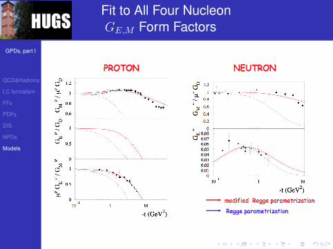
Fit to All Four NucleonGE,M Form Factors

GPDs, part I
QCD&Hadrons
LC formalism
FFs
PDFs
DIS
NPDs
Models
Fit to F1,2 Proton Form Factors
Modified Regge parametrization describes JLab polarizationtransfer data on GpE/G
pM and F p2 /F
p1
Similar model was constructed by Diehl et al. (right figure)

GPDs, part I
QCD&Hadrons
LC formalism
FFs
PDFs
DIS
NPDs
Models
Summary
1 Why Study QCD and Hadronic Structure
2 Light-cone formalism
3 Form Factors
4 Usual Parton Densities
5 Deep Inelastic Scattering
6 Nonforward Parton Densities
7 Regge-type models for NPDs