Embed Size (px)
Citation preview
MA4G6 Lecture Notes
Introduction to theModern Calculus of Variations
Filip Rindler
Spring Term 2017

Filip RindlerMathematics InstituteUniversity of WarwickCoventry CV4 7ALUnited [email protected]
http://www.warwick.ac.uk/filiprindler
Copyright ©2017 Filip Rindler.Version 2.0.
Preface
The calculus of variations has seen a sweeping renaissance since the 1970s, ignited by thediscovery of powerful variational methods to investigate nonlinear elasticity and microstruc-ture in materials. It was further fueled by the adaptation of sophisticated mathematical tech-niques from measure theory, geometric analysis, and modern PDE theory. With these fieldsnow more closely intertwined than ever, the methods of the modern calculus of variationsare now among the most powerful to study highly nonlinear problems.
These lecture notes, written for the MA4G6 Calculus of Variations course at the Univer-sity of Warwick, intend to give a modern introduction to the Calculus of Variations. I havetried to cover different aspects of the field and to explain how they fit into the “big picture”.I have tried to strike a balance between a pure introduction and a text that can be used forlater revision of forgotten material.
The presentation is based around a few principles:
• I use modern techniques and present results which are perhaps not usually found inan introductory text. I have organized the material thematically, not necessarily in theorder in which it was discovered.
• For most results, I try to use “reasonable” assumptions, not the most general ones.
• When presented with a choice of how to prove a result, I have usually chosen the (inmy opinion) most conceptually clear approach over more “elementary” ones. For in-stance, since Young measures pervade large parts of the modern theory of microstruc-ture, it is convenient to already use them for lower semicontinuity results, even thoughmore elementary approaches exist. This comes at the expense of a higher initial bur-den of abstract theory, but it gives the reader a powerful “toolbox” that can easily beapplied to a variety of problems.
• I do not attempt to trace every result to its original source.
• I consider vector-valued u right from the start since this situation has many applica-tions and, in fact, much of the advanced theory was specifically developed for thissituation.
• I occasionally refer to further results without giving a proof. The rationale behindthis is that I want the reader to see the frontier of research, without compromising the
Com
men
t...

ii PREFACE
coherence of the text. I hope the reader will take these “tasters” as motivation to readthe original papers.
This text was strongly influenced by several previous works, I note in particular thelecture notes on microstructure by Muller [85], Dacorogna’s treatise on the calculus of vari-ations [29], Kirchheim’s advanced lecture notes on differential inclusions [60], the book onYoung measures by Pedregal [94], Giusti’s more regularity theory-focused introduction tothe calculus of variations [49], Dolzmann’s book on modern aspects of microstructure [36],as well as lecture notes on several related courses by Ball, Kristensen, and Mielke.
These lecture notes are a living document and I would appreciate comments, correctionsand remarks – however small. They can be sent back to me via e-mail at
or anonymously via
http://tinyurl.com/MA4G6-2017
or by scanning the following QR-Code:
Moreover, every page contains its individual QR-code for immediate feedback. I encourageall readers to make use of them.
I would like to thank in particular my teachers Alexander Mielke and Jan Kristensen.Through their generosity and enthusiasm in sharing their knowledge they have provided mewith the foundation for my study and research. Furthermore, I am grateful to Guido DePhilippis, Richard Gratwick, Angkana Ruland, Giles Shaw, the participants of the MA4G6course at Warwick in 2015, for many helpful comments, corrections, and remarks. Finally.Finally, I would like to acknowledge the support from an EPSRC Research Fellowship on“Singularities in Nonlinear PDEs” (EP/L018934/1).
January 2017 Filip Rindler
Com
men
t...

Contents
Preface i
Contents iii
1 Introduction 11.1 The brachistochrone problem . . . . . . . . . . . . . . . . . . . . . . . . . 21.2 Electrostatics . . . . . . . . . . . . . . . . . . . . . . . . . . . . . . . . . 41.3 Stationary states in quantum mechanics . . . . . . . . . . . . . . . . . . . 51.4 Hyperelasticity . . . . . . . . . . . . . . . . . . . . . . . . . . . . . . . . 61.5 Microstructure in crystals . . . . . . . . . . . . . . . . . . . . . . . . . . . 81.6 Optimal saving and consumption . . . . . . . . . . . . . . . . . . . . . . . 101.7 Sailing against the wind . . . . . . . . . . . . . . . . . . . . . . . . . . . . 11
2 Convexity 132.1 The Direct Method . . . . . . . . . . . . . . . . . . . . . . . . . . . . . . 142.2 Functionals with convex integrands . . . . . . . . . . . . . . . . . . . . . . 162.3 Integrands with u-dependence . . . . . . . . . . . . . . . . . . . . . . . . 202.4 The Euler–Lagrange equation . . . . . . . . . . . . . . . . . . . . . . . . . 212.5 Regularity of minimizers . . . . . . . . . . . . . . . . . . . . . . . . . . . 262.6 Lavrentiev gap phenomenon . . . . . . . . . . . . . . . . . . . . . . . . . 332.7 Invariances and the Noether theorem . . . . . . . . . . . . . . . . . . . . . 362.8 Side constraints . . . . . . . . . . . . . . . . . . . . . . . . . . . . . . . . 40Notes and historical remarks . . . . . . . . . . . . . . . . . . . . . . . . . . . . 44
3 Quasiconvexity 453.1 Quasiconvexity . . . . . . . . . . . . . . . . . . . . . . . . . . . . . . . . 463.2 Null-Lagrangians . . . . . . . . . . . . . . . . . . . . . . . . . . . . . . . 533.3 Young measures . . . . . . . . . . . . . . . . . . . . . . . . . . . . . . . . 563.4 Gradient Young measures . . . . . . . . . . . . . . . . . . . . . . . . . . . 653.5 Homogeneous gradient Young measures . . . . . . . . . . . . . . . . . . . 673.6 Lower semicontinuity . . . . . . . . . . . . . . . . . . . . . . . . . . . . . 703.7 Integrands with u-dependence . . . . . . . . . . . . . . . . . . . . . . . . 753.8 Regularity of minimizers . . . . . . . . . . . . . . . . . . . . . . . . . . . 76
Com
men
t...
iv CONTENTS
Notes and historical remarks . . . . . . . . . . . . . . . . . . . . . . . . . . . . 78
4 Polyconvexity 814.1 Polyconvexity . . . . . . . . . . . . . . . . . . . . . . . . . . . . . . . . . 824.2 Existence of minimizers . . . . . . . . . . . . . . . . . . . . . . . . . . . 834.3 Global injectivity . . . . . . . . . . . . . . . . . . . . . . . . . . . . . . . 89Notes and historical remarks . . . . . . . . . . . . . . . . . . . . . . . . . . . . 91
5 Relaxation 935.1 Quasiconvex envelopes . . . . . . . . . . . . . . . . . . . . . . . . . . . . 945.2 Relaxation of integral functionals . . . . . . . . . . . . . . . . . . . . . . . 985.3 Young measure relaxation . . . . . . . . . . . . . . . . . . . . . . . . . . . 1025.4 Rigidity for gradients . . . . . . . . . . . . . . . . . . . . . . . . . . . . . 1085.5 Characterization of gradient Young measures . . . . . . . . . . . . . . . . 1115.6 Quasiconvexity versus rank-one convexity . . . . . . . . . . . . . . . . . . 115Notes and historical remarks . . . . . . . . . . . . . . . . . . . . . . . . . . . . 118
A Prerequisites 119A.1 Linear algebra . . . . . . . . . . . . . . . . . . . . . . . . . . . . . . . . . 119A.2 Measure theory . . . . . . . . . . . . . . . . . . . . . . . . . . . . . . . . 122A.3 Functional analysis . . . . . . . . . . . . . . . . . . . . . . . . . . . . . . 126A.4 Sobolev and other function spaces . . . . . . . . . . . . . . . . . . . . . . 127A.5 Harmonic analysis . . . . . . . . . . . . . . . . . . . . . . . . . . . . . . 130
Bibliography 133
Index 141
Com
men
t...
Chapter 1
Introduction
A mathematical model of some aspect of reality needs to balance its validity, that is, itsagreement with nature, and its predictive capabilities, with the feasibility of its mathematicaltreatment. In this quest to formulate a useful picture of an aspect of the world, it turns outon surprisingly many occasions that the formulation of the model becomes clearer, morecompact, or more convincing if one introduces some form of variational principle. This isthe case if one can define a quantity, such as energy or entropy, which obeys a minimization,maximization or saddle-point law.
How much we perceive such a quantity as “fundamental” depends on the situation. Forexample, in classical mechanics, one calls forces conservative if they are path-independentand hence originate from changing an “energy potential”. It turns out that many forces inphysics are conservative, which seems to imply that the concept of energy is fundamental.Furthermore, Einstein’s famous formula E = mc2 expresses the equivalence of mass andenergy, positioning energy as the “most” fundamental quantity, with mass becoming “con-densated” energy. On the other hand, the other ubiquitous scalar physical quantity, entropy,has a more “artificial” flavor as a measure of missing information in a model, as is now wellunderstood in the field of statistical mechanics, where entropy becomes a derived quantity.
Our approach to variational quantities here is a pragmatic one: We see them as providingstructure to a problem, which enables us to use powerful variational methods. For instance,in elasticity theory it is usually unrealistic that a system will tend to a global minimizer byitself, but this does not mean that – as an approximation – such a principle cannot be usefulin practice. If we wait long enough, the inherent noise in a realistic system will move oursystem around and with a high probability it will be near a low-energy state.
In this text, we focus on minimization problems for integral functionals defined on mapsfrom an open and bounded set Ω ⊂ Rd to some Rm, that is, we minimize∫
Ωf (x,u(x),∇u(x)) dx → min, u : Ω → Rm,
possibly under conditions on the boundary values of u and further side constraints. Theseproblems form the original core of the calculus of variations and are as relevant today as theyhave always been. The systematic understanding of these integral functionals starts in Eu-ler’s and Bernoulli’s times in the late 1600s and the early 1700s, and their study was boosted
Com
men
t...

2 CHAPTER 1. INTRODUCTION
into the modern age by Hilbert’s 19th, 20th, 23rd problems, formulated in 1900 [55]. Theexcitement has never stopped since and new and important discoveries are made every year.
We start by looking at a parade of examples, which we treat at varying levels of detail.All these problems will be investigated further along the course once we have developed thenecessary mathematical tools.
1.1 The brachistochrone problem
While the name “calculus of variations” is from Leonhard Euler’s 1766 treatise Elementacalculi variationum, the beginning of the field can be traced back to June 1696, when JohannBernoulli published a problem in the journal Acta Eruditorum. This “birth certificate” ofthe calculus of variations can be seen at
http://tinyurl.com/CoVbirth
or by scanning the following QR-Code:
Additionally, Bernoulli sent a letter containing the question to Gottfried Wilhelm Leibnizon 9 June 1696, who returned his solution only a few days later on 16 June, and commentedthat the problem tempted him “like the apple tempted Eve”. Isaac Newton also publisheda solution (after the problem had reached him) without giving his identity, but Bernoulliidentified him “ex ungue leonem” (from Latin, “by the lion’s claw”). The problem wasformulated as follows:
Given two points A and B in a vertical [meaning “not horizontal”] plane, oneshall find a curve AMB for a movable point M, on which it travels from A to Bin the shortest time, only driven by its own weight.
The resulting curve is called the brachistochrone (from Ancient Greek, “shortest time”)curve.
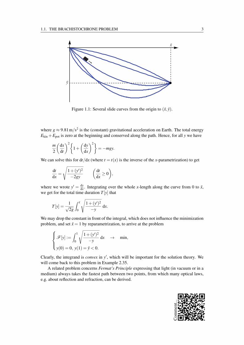
We set up the mathematical formulation as follows: We look for the curve y connectingthe origin (0,0) to the point (x, y), where x > 0, y < 0, such that a point mass m > 0 slidesfrom rest at (0,0) to (x, y) quickest among all such curves. See Figure 1.1 for severalpossible slide paths. We parametrize a point (x,y) on the curve by the time t ≥ 0. The pointmass has kinetic and potential energies
Ekin =m2
(dxdt
)2
+
(dydt
)2=
m2
(dxdt
)21+(
dydx
)2,
Epot = mgy,
Com
men
t...
1.1. THE BRACHISTOCHRONE PROBLEM 3
Figure 1.1: Several slide curves from the origin to (x, y).
where g ≈ 9.81m/s2 is the (constant) gravitational acceleration on Earth. The total energyEkin +Epot is zero at the beginning and conserved along the path. Hence, for all y we have
m2
(dxdt
)21+(
dydx
)2=−mgy.
We can solve this for dt/dx (where t = t(x) is the inverse of the x-parametrization) to get
dtdx
=
√1+(y′)2
−2gy
(dtdx
≥ 0),
where we wrote y′ = dydx . Integrating over the whole x-length along the curve from 0 to x,
we get for the total time duration T [y] that
T [y] =1√2g
∫ x
0
√1+(y′)2
−ydx.
We may drop the constant in front of the integral, which does not influence the minimizationproblem, and set x = 1 by reparametrization, to arrive at the problemF [y] :=
∫ 1
0
√1+(y′)2
−ydx → min,
y(0) = 0, y(1) = y < 0.
Clearly, the integrand is convex in y′, which will be important for the solution theory. Wewill come back to this problem in Example 2.35.
A related problem concerns Fermat’s Principle expressing that light (in vacuum or in amedium) always takes the fastest path between two points, from which many optical laws,e.g. about reflection and refraction, can be derived.
Com
men
t...
4 CHAPTER 1. INTRODUCTION
1.2 Electrostatics
Consider an electric charge density ρ : R3 → R (in units of C/m3) in three-dimensionalvacuum. Let E : R3 → R3 (in V/m) and B : R3 → R3 (in T = Vs/m2) be the electric andmagnetic fields, respectively, which we assume to be constant in time (hence electrostatics).Assuming that R3 is a linear, homogeneous, isotropic electric material, the Gauss law forelectricity reads
∇ ·E = divE =ρε0,
where ε0 ≈ 8.854 ·10−12 C/(Vm). Moreover, we have the Faraday law of induction
∇×E = curlE =dBdt
= 0.
Thus, since E is curl-free, there exist an electric potential φ : R3 → R (in V) such that
E =−∇φ.
Combining this with the Gauss law, we arrive at the Poisson equation,
∆φ = ∇ · [∇φ ] =− ρε0. (1.1)
We can also look at electrostatics in a variational way: We use the norming conditionφ(0) = 0. Then, the electric potential energy UE(x;q) of a point charge q > 0 (in C) at pointx ∈ R3 in the electric field E is given by the path integral (which does not depend on thepath chosen since E is a gradient)
UE(x;q) =−∫ x
0qE ·ds =−
∫ 1
0qE(hx) dh = qφ(x).
Thus, the total electric energy of our charge distribution ρ is (the factor 1/2 is necessary tocount mutual reaction forces correctly)
UE :=12
∫R3
ρφ dx =ε0
2
∫R3(∇ ·E)φ dx,
which has units of CV = J. Using (∇ ·E)φ = ∇ · (Eφ)−E · (∇φ), the divergence theorem,and the natural assumption that φ vanishes at infinity, we get further
UE =ε0
2
∫R3
∇ · (Eφ)−E · (∇φ) dx =−ε0
2
∫R3
E · (∇φ) dx =ε0
2
∫R3
|∇φ|2 dx.
The integral∫Ω|∇φ|2 dx
Com
men
t...

1.3. STATIONARY STATES IN QUANTUM MECHANICS 5
is called Dirichlet integral.In Example 2.15 we will see that (1.1) is equivalent to the minimization problem (over
φ)
UE −∫R3
ρφ dx =∫R3
ε0
2|∇φ |2 −ρφ dx → min .
The second term is the energy stored in the electric field caused by its interaction with thecharge density ρ .
1.3 Stationary states in quantum mechanics
The non-relativistic evolution of a quantum mechanical system with N degrees of freedomin an electrical field is described completely through its wave function Ψ : RN ×R → Cthat satisfies the Schrodinger equation
ihddt
Ψ(x, t) =[−h2
2µ∆ +V (x, t)
]Ψ(x, t), x ∈ RN , t ∈ R,
where h ≈ 1.05 · 10−34 Js is the reduced Planck constant, µ > 0 is the reduced mass, andV = V (x, t) ∈ R is the potential energy. The (self-adjoint) operator H := −(2µ)−1h∆ +Vis called the Hamiltonian of the system.
The value of the wave function itself at a given point in spacetime has no physical inter-pretation, but according to the Copenhagen Interpretation of quantum mechanics, |Ψ(x)|2is the probability density of finding a particle at the point x. In order for |Ψ|2 to be a proba-bility density, we need to impose the side constraint
∥Ψ∥L2 = 1.
In particular, Ψ(x, t) has to decay as |x| → ∞.Of particular interest are the so-called stationary states, that is, solutions of the station-
ary Schrodinger equation[−h2
2µ∆ +V (x)
]Ψ(x) = EΨ(x), x ∈ RN ,
where E > 0 is an energy level. We then solve this eigenvalue problem (in a weak sense) forΨ ∈ W1,2(RN ;C) with ∥Ψ∥L2 = 1 (see Appendix A.4 for a collection of facts about Sobolevspaces like W1,2).
If we are just interested in the lowest-energy state, the so-called ground state, we canfind minimizers of the energy functional
E [Ψ] :=∫RN
h2
2µ|∇Ψ(x)|2 + 1
2V (x)|Ψ(x)|2 dx,
again under the side constraint
∥Ψ∥L2 = 1.
The two parts of the integral above correspond to kinetic and potential energy, respectively.We will continue this investigation in Example 2.40.
Com
men
t...

6 CHAPTER 1. INTRODUCTION
1.4 Hyperelasticity
Elasticity theory is one of the most important theories of continuum mechanics, that is, thestudy of the mechanics of (idealized) continuous media. We will not go into much detailabout elasticity modeling here and refer to the book [22] for a thorough introduction.
Consider a body of mass occupying a bounded Lipschitz domain Ω ⊂ R3, that is anopen, connected set such that ∂Ω is a Lipschitz manifold (the union of finitely many Lip-schitz graphs). We call Ω the reference configuration. If we deform the body, any mate-rial point x ∈ Ω is mapped into a spatial point y(x) ∈ R3 and we call y(Ω) the deformedconfiguration. For a suitable continuum mechanics theory, we also need to require thaty : Ω → y(Ω) is a differentiable bijection and that it is orientation-preserving, i.e. that
det∇y(x)> 0 for all x ∈ Ω.
For convenience one also introduces the displacement
u(x) := y(x)− x.
One can show (using the implicit function theorem and the mean value theorem) that theorientation-preserving condition and the invertibility are satisfied if
supx∈Ω
|∇u(x)|< δ (Ω) (1.2)
for a domain-dependent (small) constant δ (Ω)> 0.Next, we need a measure of local “stretching”, called a strain tensor, which should serve
as the parameter to a local energy density. On physical grounds, rigid body motions, that is,deformations u(x)=Rx+u0 with a rotation R∈R3×3 (RT =R−1 and detR= 1) and u0 ∈R3,should not cause strain. In this sense, strain measures the deviation of the displacement froma rigid body motion. One popular choice is the Green–St. Venant strain tensor1
E :=12(∇u+∇uT +∇uT ∇u
). (1.3)
We first consider fully nonlinear (“finite strain”) elasticity. For our purposes we simplypostulate the existence of a stored-energy density W : R3×3 → [0,∞] and an external bodyforce field b : Ω → R3 (e.g. gravity) such that
F [y] :=∫
ΩW (∇y)−b · y dx
represents the total elastic energy stored in the system. If the elastic energy can be writtenin this way as∫
ΩW (∇y(x)) dx,
we call the material hyperelastic. In applications, W is often given as depending on theGreen–St. Venant strain tensor E instead of ∇y, but for our mathematical theory, the aboveform is more convenient. We require several properties of W for arguments F ∈ R3×3:
1There is an array of choices for the strain tensor, but they are mostly equivalent within nonlinear elasticity.
Com
men
t...

1.4. HYPERELASTICITY 7
(i) Norming: W (Id) = 0 (the undeformed state costs no energy).
(ii) Frame-invariance: W (RF) =W (F) for all R ∈ SO(3).
(iii) Infinite compression costs infinite energy: W (F)→+∞ as detF ↓ 0.
(iv) Infinite stretching costs infinite energy: W (F)→+∞ as |F | → ∞.
The main problem of nonlinear hyperelasticity is to minimize F as above over ally : Ω → R3 with given boundary values. Of course, it is not a-priori clear in which spacewe should look for a solution. Indeed, this depends on the growth properties of W . Forexample, for the prototypical choice
W (F) := dist(F,SO(3))2, where dist(x,K) := infy∈K
|x− y|.
However, this W does not satisfy (3) from our list of requirements, we would look forsquare integrable functions. More realistic in applications are the Mooney–Rivlin materi-als, where W is of the form
W (F) := a|F |2 +b|cofF |2 +Γ(detF),
with a,b > 0 and Γ(d) = αd2 −β logd for α,β > 0. If b = 0 the material is called neo-Hookean. An even larger class are the Ogden materials, for which
W (F) :=M
∑i=1
ai tr[(FT F)γi/2]+ N
∑j=1
b j tr cof[(FT F)δ j/2]+Γ(detF), F ∈ R3×3,
where ai > 0, γi ≥ 1, b j > 0, δ j ≥ 1, and Γ : R → R∪ +∞ is a convex function withΓ(d) → +∞ as d ↓ 0, Γ(d) = +∞ for s ≤ 0. These materials occur in a wide range ofapplications.
In the setting of linearized elasticity, we make the “small strain” assumption that thequadratic term in (1.3) can be neglected and that (1.2) holds. In this case, we work with thelinearized strain tensor
E u :=12(∇u+∇uT ).
In this infinitesimal deformation setting, the displacements that do not create strain areprecisely the skew-affine maps2 u(x) = Qx+u0 with QT =−Q and u0 ∈ R.
For linearized elasticity we consider an energy of the special “quadratic” form
F [u] :=∫
Ω
12E u : CE u−b ·u dx,
2This becomes more meaningful when considering a bit more algebra: The Lie group SO(3) of rotationshas as its Lie algebra Lie(SO(3)) = so(3) the space of all skew-symmetric matrices, which then can be seen as“infinitesimal rotations”.
Com
men
t...

8 CHAPTER 1. INTRODUCTION
where C(x) = Ci jkl(x) is a symmetric, strictly positive definite (A : C(x)A > c|A|2 for somec > 0) fourth-order tensor, called the elasticity/stiffness tensor, and b : Ω → R3 is ourexternal body force. Thus we will always look for solutions in W1,2(Ω;R3).
For homogeneous, isotropic media, C does not depend on x or the direction of strain,which translates into the additional condition
(AR) : C(x)(AR) = A : C(x)A for all x ∈ Ω, A ∈ R3×3 and R ∈ SO(3).
In this case, it can be shown that F simplifies to
F [u] =12
∫Ω
2µ|E u|2 +(
κ − 23
µ)| trE u|2 −b ·u dx
for µ > 0 the shear modulus and κ > 0 the bulk modulus, which are material constants. Forexample, for cold-rolled steel µ ≈ 75 GPa and κ ≈ 160 GPa.
1.5 Microstructure in crystals
Consider a material specimen with internal crystal structure, for instance a metal (like iron)or an alloy (like CuAlNi). We assume that all atoms are arranged in the same single crystaloccupying an (open, bounded) reference domain Ω ⊂ Rd , where d = 2 (plates) or d =3. If we subject our specimen to external forces or push it into a prescribed shape at theboundary, we want to determine the resulting shape. It turns out that on a microscopic scalecrystals often display very fine oscillations between different phases, that is, the crystalexhibits locally periodic fine structures. It turns out that this microstructure has profoundimplications for the macroscopic behavior of the material. Usually, the phase oscillationsdo not reach atomic length scales, so we can still attempt to model our situation usingcontinuum mechanics.
The fundamental Cauchy–Born hypothesis3 postulates that for small linear displace-ments the crystal lattice atoms will follow this displacement. Assuming this, we can modelthe crystal as a continuum and assign the energy density W (F)≥ 0 to the linear deformationx 7→ Fx. The crucial point here is that, thanks to the Cauchy–Born hypothesis, W dependsonly on F and no other “microscopic structure” of the crystal, at least for small to moderatecrystal deformations. Then, in this approach, the total energy of a deformation u : Ω → R3
is given as
F [u] :=∫
ΩW (∇u(x)) dx, u : Ω → R3.
Here, on W : R3×3 → [0,∞) we make the following assumptions:
(i) Norming: W (Id) = 0 (the undeformed state costs no energy).
(ii) Frame-invariance: W (RF) =W (F) for all R ∈ SO(3).
3This assumption is often made, but is not always justified, see [26, 38, 40, 46].
Com
men
t...
1.5. MICROSTRUCTURE IN CRYSTALS 9
(iii) Symmetry-invariance: W (FS) =W (S) for all S ∈S , where S ⊂ SO(3) is the com-pact symmetry point group of the crystal.
The basic variational postulate is now that the observed macroscopic deformation is aminimizer of F under the given boundary conditions. In fact, it is often experimentally ob-served that the observed deformation u : Ω →R3 is a pointwise minimizer of the integrand,at least in a very large portion of Ω. Thus, we are led to consider the differential inclusion
∇u(x) ∈ K :=
A ∈ R3×3 : W (A) = minW=W−1(0) a.e.
The set K is usually compact in the study of crystal, but other applications also lead to theseinclusions for non-compact K.
For concrete crystals one often observes the following situation: Above a critical tem-perature, K is simply SO(d), i.e. the simplest possible set that is compatible with the frame-invariance (ii) above. This is called the cubic phase. Passing through the critical tempera-ture, however, the material undergoes a solid–solid phase transition and K is now the unionof several wells, that is,
K = SO(d)U1 ∪·· ·∪SO(d)UN
for distinct matrices U1, . . . ,UN ∈ Rd×d with detUi > 0 (i = 1, . . . ,N). By the polar de-composition of matrices with positive determinants into the product of a rotation and asymmetric positive definite matrix, we can assume that
Ui is symmetric and positive definite, i = 1, . . . ,N.
If N ≥ 2 and other compatibility conditions between the U j are satisfied, microstructurecan be observed. It should be noted that while our model as formulated above may imply“infinitely fast” oscillations in the microstructure, in reality other (atomistic) effects limitthe length scales that are observed.
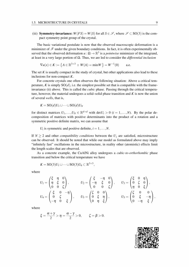
As a concrete example, the CuAlNi alloy undergoes a cubic-to-orthorhombic phasetransition and below the critical temperature we have
K = SO(3)U1 ∪·· ·∪SO(3)U6 ⊂ R3×3,
where
U1 =
ξ η 0η ξ 00 0 ζ
, U2 =
ξ −η 0−η ξ 00 0 ζ
, U3 =
ξ 0 η0 ζ 0η 0 ξ
,
U4 =
ξ 0 −η0 ζ−η 0 ξ
, U5 =
ζ 0 00 ξ η0 η ξ
, U5 =
ζ 0 00 ξ −η0 −η ξ
,
where
ξ =α + γ
2> η =
α − γ2
> 0, ζ = β > 0.
Com
men
t...

10 CHAPTER 1. INTRODUCTION
Depending on the choice of values of the parameters, a large variety of microstructure vari-ation is observed.
One striking property of CuAlNi is the shape-memory effect, where a material specimen“remembers” the shape it had when it was hotter than a certain critical temperature. Aftercooling, the specimen can be freely deformed, but when it is again heated above the criticaltemperature, it “snaps back” into its orginal shape.
In this work we will only consider the basic principles underlying this problem, concreteapplications are left to more specialized treatises like [36] (in particular, Section 5.3 in loc.cit. in relation to the above example of CuAlNi).
1.6 Optimal saving and consumption
Consider a capitalist worker earning a (constant) wage w per year, which he can either spendon consumption or save. Denote by S(t) the savings at time t, where t ∈ [0,T ] is in years,with t = 0 denoting the beginning of his work life and t = T his retirement. Further, letC(t) be the consumption rate (consumption per time) at time t. On the saved capital, theworker earns interest, say with gross-continuous rate ρ > 0, meaning that a capital amountm > 0 grows as exp(ρt)m. If we were given an APR ρ1 > 0 instead of ρ , we could computeρ = ln(1+ ρ1). We further assume that salary is paid continuously, not in intervals, forsimplicity. So, w is really the rate of pay, given in money per time. Then, the worker’ssavings evolve according to the differential equation
S(t) = w+ρS(t)−C(t). (1.4)
Now, assume that our worker is mathematically inclined and wants to optimize thehappiness due to consumption in his life by finding the optimal amount of consumptionat any given time. Being a pure capitalist, the worker’s happiness only depends on hisconsumption rate C. So, if we denote by U(C) the utility function, that is, the “happiness”due to the consumption rate C, our worker wants to find C : [0,T ]→ R such that
H [C] :=∫ T
0U(C(t)) dt
is maximized. The choice of U depends on our worker’s personality, but it is probably real-istic to assume that there is a law of diminishing returns, i.e. for twice as much consumption,our worker is happier, but not twice as happy. So, let us assume U ′ > 0 and U ′(C)→ 0 asC → ∞. Also, we should have U(0) = −∞ (starvation). Moreover, it is realistic for U tobe concave, which implies that there are no local maxima. One function that satisfies all ofthese requirements is the logarithm, and so we use
U(C) = ln(C), C > 0.
Let us also assume that the worker starts with no savings, S(0) = 0, and at the endof his work life wants to retire with savings S(T ) = ST ≥ 0. Rearranging (1.4) for C(t)
Com
men
t...

1.7. SAILING AGAINST THE WIND 11
and plugging this into the formula for H , we therefore want to solve the optimal savingproblemF [S] :=
∫ T
0− ln(w+ρS(t)− S(t)) dt → min,
S(0) = 0, S(T ) = ST ≥ 0.
This will be solved in Example 2.18.
1.7 Sailing against the wind
Every sailor knows how to sail against the wind by “beating”: One has to sail at an angle ofapproximately 45 to the wind4, then tack (turn the bow through the wind) and finally, afterthe sail has caught the wind on the other side, continue again at approximately 45 to thewind. Repeating this procedure makes the boat follow a zig-zag motion, which gives a netmovement directly against the wind, see Figure 1.2. A mathematically inclined sailor mightask the question of “how often to tack”. In an idealized model we can assume that tackingcosts no time and that the forward sailing speed vs of the boat depends on the angle α to thewind as follows (at least qualitatively):
vs(α) =−cos(4α),
which has maxima at α =±45 (in real boats, the maximum might be at a lower angle, i.e.“closer to the wind”). Assume furthermore that our sailor is sailing along a straight riverwith the current. Now, the current is fastest in the middle of the river and goes down to zeroat the banks. In fact, a good approximation would be the formula of Poiseuille (channel)flow, which can be derived from the flow equations of fluids: At distance r from the centerof the river the current’s flow speed is approximately
vc(r) := vmax
(1− r2
R2
),
where R > 0 is half the width of the river.If we denote by r(t) the distance of our boat from the middle of the channel at time
t ∈ [0,T ], then the total speed (called the “velocity made good” in sailing parlance) is
v(t) := vs(arctanr′(t))+ vc(r(t))
=−cos(4arctanr′(t))+ vmax
(1− r(t)2
R2
).
The key to understand this problem is now the fact that a 7→ −cos(4arctana) has two max-ima at a =±1. We say that this function is a double-well potential.
4The optimal angle depends on the boat. Ask a sailor about this and you will get an evening-filling lecture.
Com
men
t...

12 CHAPTER 1. INTRODUCTION
Figure 1.2: Sailing against the wind in a channel.
The total forward distance traveled over the time interval [0,T ] is∫ T
0v(t) dt =
∫ T
0−cos(4arctanr′(t))+ vmax
(1− r(t)2
R2
)dt.
If we also require the initial and terminal conditions r(0) = r(T ) = 0, we arrive at theoptimal beating problem:F [r] :=
∫ T
0cos(4arctanr′(t))− vmax
(1− r(t)2
R2
)dt → min,
r(0) = r(T ) = 0, |r(t)| ≤ R.
Our intuition tells us that in this idealized model, where tacking costs no time, we shouldbe tacking as “infinitely fast” in order to stay in the middle of the river. Later, once we haveadvanced tools at our disposal, we will make this idea precise, see Example 5.7.
Com
men
t...

Chapter 2
Convexity
In the introduction we got a glimpse of the many applications of minimization problems inphysics, technology, and economics. In this chapter we start to develop the mathematicaltheory that will allow us to investigate these problems. Consider a minimization problem ofthe formF [u] :=
∫Ω
f (x,u(x),∇u(x)) dx → min,
over all u ∈ W1,p(Ω;Rm) with u|∂Ω = g.
Here, and throughout the text (if not otherwise stated) we will make the standard assump-tion that Ω ⊂ Rd is a bounded Lipschitz domain, that is, Ω is open, bounded, and has aboundary that is the union of finitely many Lipschitz manifolds. The function
f : Ω×Rm ×Rm×d → R,
is required to be measurable in the first and continuous in the second and third arguments,hence f is a so-called Caratheodory integrand. Furthermore, in this chapter we let 1 <p < ∞ and on the prescribed boundary values g we assume
g ∈ W1−1/p,p(∂Ω;Rm).
In this context recall that W1−1/p,p(∂Ω;Rm) is the space of traces of all Sobolev functionsu ∈ W1,p(Ω;Rm), see Appendix A.4 for some background on Sobolev spaces. Furthermore,to make the above integral finite, we assume the p-growth bound
| f (x,v,A)| ≤ M(1+ |v|p + |A|p) (x,v,A) ∈ Ω×Rm ×Rm×d ,
for some M > 0.Below, we will investigate the solvability and regularity properties of this minimization
problem; in particular, we will take a close look at the way in which convexity propertiesof f in its gradient (third) argument determine whether F is lower semicontinuous, whichis the decisive attribute in the fundamental Direct Method of the calculus of variations.
Com
men
t...
14 CHAPTER 2. CONVEXITY
We will also consider the partial differential equation associated with the minimizationproblem, the so-called Euler–Lagrange equation, which constitutes a necessary, but notsufficient, condition for minimizers. This leads naturally to the question of regularity ofsolutions. Finally, we also treat invariances, leading to the famous Noether theorem beforehaving a glimpse at side constraints.
2.1 The Direct Method
Fundamental to all of the existence theorems in this text is the conceptionally simple DirectMethod of the calculus of variations, which is “direct” since we prove the existence ofsolutions to minimization problems without the detour through a differential equation. LetX be a complete metric space (e.g. a Banach space with the norm topology or a closed,convex and bounded subset of a Banach space with the weak or weak* topology) and letF : X → R∪+∞ be our objective functional satisfying the following two assumptions:
(H1) Coercivity: For all Λ ∈ R, the sublevel set u ∈ X : F [u]≤ Λ is sequentially rel-atively compact, that is, if F [u j]≤ Λ for a sequence (u j)⊂ X and some Λ ∈ R, then(u j) has a convergent subsequence in X .
(H2) Lower semicontinuity: For all sequences (u j)⊂ X with u j → u it holds that
F [u]≤ liminfj→∞
F [u j].
The Direct Method for the abstract minimization problem
F [u]→ min over all u ∈ X . (2.1)
is encapsulated in the following simple result:
Theorem 2.1 (Direct Method). Assume that F is both coercive and lower semicontinu-ous. Then, the abstract minimization problem (2.1) has at least one solution, that is, thereexists u∗ ∈ X with F [u∗] = minF [u] : u ∈ X .
Proof. Let us assume that there exists at least one u ∈ X such that F [u] < +∞; otherwise,any u ∈ X is a “solution” to the (degenerate) minimization problem.
To construct a minimizer we take a minimizing sequence (u j)⊂ X such that
limj→∞
F [u j]→ α := inf
F [u] : u ∈ X<+∞.
Then, since convergent sequences are bounded, there exists Λ ∈ R such that F [u j]≤ Λ forall j ∈N. Hence, by the coercivity (H1), the sequence (u j) is contained in a compact subsetof X . Now select a subsequence, which here as in the following we do not renumber, suchthat
u j → u∗ ∈ X .
Com
men
t...

2.1. THE DIRECT METHOD 15
By the lower semicontinuity (H2), we immediately conclude
α ≤ F [u∗]≤ liminfj→∞
F [u j] = α.
Thus, F [u∗] = α and u∗ is the sought minimizer.
Example 2.2. Using the Direct Method, one can easily see that
h(t) :=
1− t if t < 0,t if t ≥ 0,
t ∈ R (= X),
has the minimizer t = 0, despite not even being continuous there.
Despite its nearly trivial proof, the Direct Method is very useful and flexible in applica-tions. Indeed, it pushes the difficulty in proving existence of a minimizer toward establishingcoercivity and lower semicontinuity. This, however, is a big advantage, since we have manytools at our disposal to establish these two hypotheses separately. In particular, for integralfunctionals, lower semicontinuity is tightly linked to convexity properties of the integrand,as we will see throughout this book.
At this point it is crucial to observe how coercivity and lower semicontinuity interactwith the topology in X : If we choose a stronger topology, i.e. one for which there arefewer convergent sequences, then it becomes easier for F to be lower semicontinuous, butharder for F to be coercive. The opposite holds if choosing a weaker topology. In themathematical treatment of a problem we are most likely in a situation where F and X aregiven by the concrete problem. We then need to find a suitable topology in which we canestablish both coercivity and lower semicontinuity.
In this text, X will always be an infinite-dimensional Banach space and we have a realchoice between using the strong or weak convergence. Usually, it turns out that coerciv-ity with respect to the strong convergence is false since strongly compact sets in infinite-dimensional spaces are very restricted, whereas coercivity with respect to the weak conver-gence is true under reasonable assumptions. However, whereas strong lower semicontinuityposes few challenges, lower semicontinuity with respect to weakly converging sequencesis a delicate matter and we will spend considerable time on this topic. As a result of thisdiscussion, we will always use the Direct Method in the following version:
Theorem 2.3 (Direct Method for weak convergence). Let X be a Banach space and letF : X → R∪+∞. Assume the following:
(WH1) Weak Coercivity: For all Λ ∈ R, the sublevel set
u ∈ X : F [u]≤ Λ is sequentially weakly relatively compact,
that is, if F [u j] ≤ Λ for a sequence (u j) ⊂ X and some Λ ∈ R, then (u j) has aweakly convergent subsequence.
Com
men
t...
16 CHAPTER 2. CONVEXITY
(WH2) Weak lower semicontinuity: For all sequences (u j)⊂ X with u j u (weak conver-gence X) it holds that
F [u]≤ liminfj→∞
F [u j].
Then, the minimization problem
F [u]→ min over all u ∈ X,
has at least one solution.
Before we move on to the more concrete theory, let us record one further remark: Whileit might appear as if “nature does not give us the topology” and it is up to mathematicians to“invent” a suitable one, it is remarkable that the topology that turns out to be mathematicallyconvenient is also often physically relevant. This is for instance expressed in the followingobservation: The only phenomena which are present in weakly but not strongly convergingsequences of Sobolev functions are oscillations and concentrations, as can be seen in theclassical Vitali Convergence Theorem A.7.
2.2 Functionals with convex integrands
As a first instance of the theory of integral functionals to be developed in this text, we firstconsider the minimization problem for the simpler functional
F [u] :=∫
Ωf (x,∇u(x)) dx
over all u∈W1,p(Ω;Rm) for some 1< p<∞ to be chosen later (depending on lower growthproperties of f ). The following lemma together with (2.3) below allows us to conclude thatF [u] is indeed well-defined.
Lemma 2.4. Let f : Ω×RN → R be a Caratheodory integrand, that is,
(i) x 7→ f (x,A) is Lebesgue-measurable for all fixed A ∈ RN .
(ii) A 7→ f (x,A) is continuous for all fixed x ∈ Ω.
Then, for any Lebesgue-measurable function V : Ω → RN the composition x 7→ f (x,V (x))is Lebesgue-measurable.
We will prove this lemma via the following “Lusin-type” theorem for Caratheodoryfunctions:
Theorem 2.5 (Scorza Dragoni 1948). Let f : Ω×RN →R be Caratheodory. Then, thereexists an increasing sequence of compact sets Sk ⊂ Ω (k ∈ N) with |Ω \ Sk| ↓ 0 such thatf |Sk×RN is continuous.
Com
men
t...

2.2. FUNCTIONALS WITH CONVEX INTEGRANDS 17
See Theorem 6.35 in [43] for a proof, which is rather measure-theoretic and similar tothe proof of the Lusin theorem, cf. Theorem 2.24 in [97].
Proof of Lemma 2.4. Let Sk ⊂ Ω (k ∈ N) be as in the Scorza Dragoni Theorem. Set fk :=f |Sk×RN and
gk(x) := fk(x,V (x)), x ∈ Sk.
Then, for any open set U ⊂ R, the pre-image of U under gk is the set of all x ∈ Sk such thatfk(x,V (x)) ∈U . As fk is continuous, f−1
k (U) is open and from the Lebesgue measurabilityof the product function x 7→ (x,V (x)) we infer that g−1
k (U) is a Lebesgue-measurable subsetof Sk. We can extend the definition of gk to all of Ω by setting gk(x) := 0 whenever x ∈Ω \ Sk. This function is still Lebesgue-measurable as Sk is compact, hence measurable.The conclusion then follows from the fact that gk(x)→ f (x,V (x)) and pointwise limits ofLebesgue-measurable functions are Lebesgue-measurable.
We next investigate coercivity: Let 1 < p < ∞. The most basic assumption to guaranteecoercivity, and the only one we want to consider here, is the following lower p-coercivitybound:
µ|A|p −µ−1 ≤ f (x,A) (x,A) ∈ Ω×Rm×d, (2.2)
for some µ > 0. This coercivity also suggests the exponent p for the definition of thefunction spaces where we look for solutions. We further assume the upper p-growth bound
| f (x,A)| ≤ M(1+ |A|p) (x,A) ∈ Ω×Rm×d , (2.3)
for some M > 0, which gives finiteness of F [u] for all u ∈ W1,p(Ω;Rm).
Proposition 2.6. If f satisfies the lower growth bound (2.2), then F is weakly coercive onthe space W1,p
g (Ω;Rm) =
u ∈ W1,p(Ω;Rm) : u|∂Ω = g
.
Proof. We need to show that any sequence (u j)⊂ W1,pg (Ω;Rm) with
sup j F [u j]< ∞
is weakly relatively compact. From (2.2) we get
µ · sup j
∫Ω|∇u j|p dx− |Ω|
µ≤ sup j F [u j]< ∞,
whereby sup j ∥∇u j∥Lp < ∞. By the Poincare–Friedrichs inequality, Theorem A.21 (i), inconjunction with the fact that we fix the boundary values, we therefore get sup j ∥u j∥W1,p <
∞. Bounded sets in reflexive Banach spaces, like W1,p(Ω;Rm) for 1 < p < ∞, are sequen-tially weakly relatively compact, see Theorem A.15, which gives the conclusion.
Com
men
t...

18 CHAPTER 2. CONVEXITY
Having settled the question of (weak) coercivity, we can now turn to investigate theweak lower semicontinuity.
Theorem 2.7. If A 7→ f (x,A) is convex for all x∈Ω and f (x,A)≥ κ for some κ ∈R (whichfollows in particular from (2.2)), then F is weakly lower semicontinuous on W1,p(Ω;Rm).
Proof. Step 1. We first establish that F is strongly lower semicontinuous, so let u j → uin W1,p and ∇u j → ∇u almost everywhere, which holds after selecting a subsequence (notrelabeled), see Appendix A.2. By assumption we have
f (x,∇u j(x))−κ ≥ 0.
Applying Fatou’s Lemma,
liminfj→∞
(F [u j]−κ|Ω|
)≥ F [u]−κ|Ω|.
Thus, F [u] ≤ liminf j→∞ F [u j]. Since this holds for all subsequences, it also follows forour original sequence.
Step 2. To prove the claimed weak lower semicontinuity take (u j)⊂ W1,p(Ω;Rm) withu j u. We need to show that
F [u]≤ liminfj→∞
F [u j] =: α. (2.4)
Taking a subsequence (not relabeled), we can in fact assume that F [u j] converges to α .By the Mazur Lemma A.18, we may find convex combinations
v j =N( j)
∑n= j
θ j,nun, where θ j,n ∈ [0,1] andN( j)
∑n= j
θ j,n = 1,
such that v j → u strongly. Since f (x, q) is convex,
F [v j] =∫
Ωf
(x,
N( j)
∑n= j
θ j,n∇un(x)
)dx ≤
N( j)
∑n= j
θ j,nF [un].
Now, F [un]→ α as n → ∞. Thus,
liminfj→∞
F [v j]≤ liminfj→∞
F [u j] = α.
On the other hand, from the first step and v j → u strongly, we have F [u]≤ liminf j→∞ F [v j].Thus, (2.4) follows and the proof is finished.
We can summarize our findings in the following theorem:
Theorem 2.8. Let f : Ω×Rm×d be a Caratheodory integrand such that f satisfies thelower growth bound (2.2), the upper growth bound (2.3) and is convex in its second argu-ment. Then, the associated functional F has a minimizer over the space W1,p
g (Ω;Rm).
Com
men
t...
2.2. FUNCTIONALS WITH CONVEX INTEGRANDS 19
Proof. This follows immediately from the Direct Method for the weak convence, Theo-rem 2.3, together with Proposition 2.6 and Theorem 2.7.
Example 2.9. The Dirichlet integral (functional) is
F [u] :=12
∫Ω|∇u(x)|2 dx, u ∈ W1,2(Ω).
We already encountered this integral functional when considering electrostatics in Sec-tion 1.2. It is easy to see that this functional satisfies all requirements of Theorem 2.8and so there exists a minimizer for any prescribed boundary values g ∈ W1/2,2(∂Ω).
Example 2.10. In the prototypical problem of linearized elasticity from Section 1.4, weare tasked with the minimization problemF [u] :=
12
∫Ω
2µ|E u|2 +(
κ − 23
µ)| trE u|2 − f ·u dx → min,
over all u ∈ W1,2(Ω;R3) with u|∂Ω = g,
where µ,κ > 0, f ∈ L2(Ω;R3), and g ∈ W1/2,2(∂Ω;Rm). It is clear that F has quadraticgrowth. Let us first consider the coercivity: For u ∈ W1,2(Ω;R3) with u|∂Ω = g we have theL2-Korn inequality
∥u∥2W1,2 ≤CK
(∥E u∥2
L2 +∥g∥2W1/2,2
). (2.5)
Here, CK = CK(Ω) > 0 is a constant. Let us for simplicity assume that κ − 23 µ ≥ 0 (this
is not necessary, but shortens the argument). Then, also using the Young inequality (seeAppendix A.1), we get for any δ > 0,
F [u]≥ µ∥E u∥2L2 −∥ f∥L2∥u∥L2
≥ µ(∥E u∥2
L2 +∥g∥2W1/2,2
)− 1
2δ∥ f∥2
L2 −δ2∥u∥2
L2 −µ∥g∥2W1/2,2
≥(
µCK
− δ2
)∥u∥2
W1,2 −1
2δ∥ f∥2
L2 −µ∥g∥2W1/2,2 .
Choosing δ = µ/CK , we obtain the coercivity estimate
F [u]≥ µ2CK
∥u∥2W1,2 −
CK
2µ∥ f∥2
L2 −µ∥g∥2W1/2,2 .
Hence, F [u] controls ∥u∥W1,2 and our functional is weakly coercive. Moreover, it is clearthat our integrand is convex in in the E u-argument (note that the trace function is linear).Hence, Theorem 2.8 yields the existence of a solution u∗ ∈W1,2(Ω;R3) to our minimizationproblem of linearized elasticity.
We finish this section with the following converse to Theorem 2.7:
Com
men
t...
20 CHAPTER 2. CONVEXITY
Proposition 2.11. Let F be an integral functional with a Caratheodory integrand f : Ω×Rm×d → R satisfying the upper growth bound (2.3). Assume furthermore that F is weaklylower semicontinuous on W1,p(Ω;Rm). If either m = 1 or d = 1 (the scalar case), thenA 7→ f (x,A) is convex for almost every x ∈ Ω.
We will not prove this result here, since Proposition 3.31 together with Corollary 3.4 inthe next chapter will give a stronger version.
In the vectorial case, i.e. m = 1 or d = 1, the necessity of convexity is far from beingtrue and there is indeed another “canonical” condition ensuring weak lower semicontinuity,which is weaker than (ordinary) convexity; we will explore this in the next chapter.
2.3 Integrands with u-dependence
If we try to extend the results in the previous section to more general functionals
F [u] :=∫
Ωf (x,u(x),∇u(x)) dx → min,
we discover that our proof strategy of using the Mazur Lemma runs into difficulties: Wecannot “pull out” the convex combination inside
∫Ω
f
(x,
N( j)
∑n= j
θ j,nun(x),N( j)
∑n= j
θ j,n∇un(x)
)dx
anymore. Nevertheless, a lower semicontinuity result analogous to the one for the scalarcase turns out to be true:
Theorem 2.12. Let f : Ω×Rm ×Rm×d → R satisfy the growth bound
| f (x,v,A)| ≤ M(1+ |v|p + |A|p) for some M > 0, 1 < p < ∞,
and the convexity property
A 7→ f (x,v,A) is convex for all (x,v) ∈ Ω×Rm.
Then, the functional
F [u] :=∫
Ωf (x,u(x),∇u(x)) dx, u ∈ W1,p(Ω;Rm),
is weakly lower semicontinuous.
While it would be possible to give an elementary proof of this theorem here, we post-pone the verification until the next chapter. There, using more advanced and elegant tech-niques (in particular Young measures), we will establish a much more general result and seethat, when viewed from the right perspective, u-dependence does not pose any additionalcomplications.
Com
men
t...

2.4. THE EULER–LAGRANGE EQUATION 21
2.4 The Euler–Lagrange equation
In analogy to the elementary fact that the derivative of a function at its minimizers is zero,we will now derive a necessary condition for a function to be a minimizer. This conditionfurnishes the connection between the calculus of variations and PDE theory and is of greatimportance for computing particular solutions.
Theorem 2.13 (Euler–Lagrange equation). Assume that f : Ω×Rm ×Rm×d → R is aCaratheodory integrand that is continuously differentiable in v and A and satisfies thegrowth bounds
|Dv f (x,v,A)|, |DA f (x,v,A)| ≤ M(1+ |v|p + |A|p), (x,v,A) ∈ Ω×Rm ×Rm×d ,
for some M > 0 and 1 ≤ p < ∞. If u∗ ∈ W1,pg (Ω;Rm), where g ∈ W1−1/p,p(∂Ω;Rm), mini-
mizes the functional
F [u] :=∫
Ωf (x,u(x),∇u(x)) dx, u ∈ W1,p
g (Ω;Rm),
then u∗ is a weak solution of the following system of PDEs, called the Euler–Lagrangeequation,
−div[DA f (x,u,∇u)
]+Dv f (x,u,∇u) = 0 in Ω,
u = g on ∂Ω.(2.6)
Here we used the common convention to omit the x-arguments whenever this does notcause any confusion in order to curtail the proliferation of x’s, for example in f (x,u,∇u) =f (x,u(x),∇u(x)). Note that our Euler–Lagrange “equation” is actually a system of PDEs.
Recall that u∗ is a weak solution of (2.6) if∫Ω
DA f (x,u∗,∇u∗) : ∇ψ +Dv f (x,u∗,∇u∗) ·ψ dx = 0
for all ψ ∈ C∞c (Ω;Rm), where DA f (x,v,A) is the matrix in Rm×d such that
DA f (x,v,A) : B = limh↓0
f (x,v,A+hB)− f (x,v,A)h
, A,B ∈ Rm×d ,
called the directional derivative of f (x,v, q) at A in direction B; here we use the Frobeniusmatrix vector product “:” (see the appendix). A similar definition applies for Dv f (x,v,A) ·w.More precisely, DA f (x,v,A) and Dv f (x,v,A) are given as
DA f (x,v,A) :=(∂A j
kf (x,v,A)
) jk, Dv f (x,v,A) :=
(∂v j f (x,v,A)
) j.
The boundary condition u = g on ∂Ω is to be understood in the sense of trace.
Com
men
t...

22 CHAPTER 2. CONVEXITY
Proof. For all ψ ∈ C∞c (Ω;Rm) and all h > 0 we have
F [u∗]≤ F [u∗+hψ]
since u∗+hψ ∈ W1,pg (Ω;Rm) is admissible in the minimization. Thus,
0 ≤∫
Ω
f (x,u∗+hψ,∇u∗+h∇ψ)− f (x,u∗,∇u∗)h
dx
=∫
Ω
∫ 1
0
1h
ddt
[f (x,u∗+ thψ,∇u∗+ th∇ψ)
]dt dx
=∫
Ω
∫ 1
0DA f (x,u∗+ thψ,∇u∗+ th∇ψ) : ∇ψ
+Dv f (x,u∗+ thψ,∇u∗+ th∇ψ) ·ψ dt dx.
By the growth bounds on the derivative, the integrand can be seen to have an h-uniform L1-majorant, namely C(1+ |u∗|p + |ψ|p + |∇u∗|p + |∇ψ|p) (if we additionally assume h ≤ 1)and so we may apply the Lebesgue dominated convergence theorem to let h ↓ 0 under thedouble integral. This yields
0 ≤∫
ΩDA f (x,u∗,∇u∗) : ∇ψ +Dv f (x,u∗,∇u∗) ·ψ dx
and we conclude by taking ψ and −ψ in this inequality.
Remark 2.14. If we want to allow ψ ∈ W1,p0 (Ω;Rm) in the weak formulation of (2.6),
then we need to assume the stronger growth conditions
|Dv f (x,v,A)|, |DA f (x,v,A)| ≤ M(1+ |v|p−1 + |A|p−1)
for some M > 0 and 1 ≤ p < ∞.
Example 2.15. Returning to the Dirichlet integral from Example 2.9, we see that the as-sociated Euler–Lagrange equation is the Laplace equation
−∆u = 0,
where ∆ := ∂ 2x1+ · · ·+∂ 2
xdis the Laplace operator. Solutions u are called harmonic func-
tions. Since the Dirichlet integral is convex, all solutions of the Laplace equation are in factminimizers. In particular, it can be seen that solutions of the Laplace equation are uniquefor given boundary values. The same results apply to the functional
F [u] :=∫
Ω
12|∇u(x)|2 −g(x) ·u(x) dx, u ∈ W1,2(Ω),
where g ∈ L2(Ω). Here, the Euler–Lagrange equation is the Poisson equation
−∆u = g.
Com
men
t...

2.4. THE EULER–LAGRANGE EQUATION 23
Example 2.16. In the linearized elasticity problem from Example 2.10, we may computethe Euler–Lagrange equation as−div
[2µ E u+
(κ − 2
3µ)(trE u)I
]= f in Ω,
u = g on ∂Ω.
Sometimes, one also defines the first variation δF [u] of F at u ∈ W1,p(Ω;Rm) as thelinear map δF [u] : W1,p
0 (Ω;Rm)→ R given as
δF [u][ψ] := limh↓0
F [u+hψ]−F [u]h
, ψ ∈ W1,p0 (Ω;Rm),
assuming this limit exists. Then, the assertion of the previous theorem can equivalently beformulated as
δF [u∗] = 0 if u∗ minimizes F over W1,pg (Ω;Rm).
Of course, this condition is only necessary for u to be a minimizer. Indeed, any solution ofthe Euler–Lagrange equation is called a critical point of F , which could be a minimizer,maximizer, or saddle point.
One crucial consequence of the results in this section is that usually we can use allavailable PDE methods to study minimizers. Immediately, one can ask about the type ofPDE we are dealing with. In this respect we have the following result:
Proposition 2.17. Let f be twice continuously differentiable in v and A. Also let A 7→f (x,v,A) be convex for all (x,v)∈Ω×Rm. Then, the Euler–Lagrange equation is an ellipticPDE, that is,
0 ≤ D2A f (x,v,A)[B,B] :=
d2
dt2 f (x,v,A+ tB)∣∣∣∣t=0
for all x ∈ Ω, v ∈ Rm, and A,B ∈ Rm×d .
The proof is immediate from the convexity.One main use of the Euler–Lagrange equation is to find concrete solutions of variational
problems:
Example 2.18. Recall the optimal saving problem from Section 1.6,F [S] :=∫ T
0− ln(w+ρS(t)− S(t)) dt → min,
S(0) = 0, S(T ) = ST ≥ 0.
The Euler–Lagrange equation is
− ddt
[1
w+ρS(t)− S(t)
]=− ρ
w+ρS(t)− S(t),
Com
men
t...
24 CHAPTER 2. CONVEXITY
which resolves to
ρ S(t)− S(t)w+ρS(t)− S(t)
= ρ .
With the consumption rate C(t) := w+ρS(t)− S(t), this is equivalent to
C(t)C(t)
= ρ,
and so, if C(0) =C0 (to be determined later),
w+ρS(t)− S(t) =C(t) = eρtC0.
This differential equation for S(t) can be solved, for example via the Duhamel formula,which yields
S(t) = eρt ·0+∫ t
0eρ(t−s)(w− eρsC0) ds
=eρt −1
ρw− teρtC0.
and C0 can now be chosen to satisfy the terminal condition S(T ) = ST , in fact, C0 = (1−e−ρT )w/(ρT )− e−ρT ST/T .
Since C 7→ − lnC is convex, we know that S(t) as above is a minimizer of our problem.In Figure 2.1 we see the optimal savings strategy for a worker earning a (constant) salaryof w = £30,000 per year and having a savings goal of ST = £100,000. The worker has tosave for approximately 27 years, reaching savings of just over £168,000, and then startswithdrawing his savings (S(t)< 0) for the last 13 years. The worker’s consumption C(t) =eρtC0 goes up continuously during the whole working life, making him/her (materially)happy.
Example 2.19. For functions u = u(t,x) : R×Rd → R, consider the action functional
A [u] :=12
∫R×Rd
−|∂tu|2 + |∇xu|2 d(t,x),
where ∇xu is the gradient of u with respect to x ∈Rd . This functional should be interpretedas the usual Dirichlet integral, see Example 2.9, where, however, we use the Lorentz metric.Then, the Euler–Lagrange equation is the wave equation
∂ 2t u−∆u = 0.
Notice that A is not convex and consequently the wave equation is hyperbolic instead ofelliptic.
Com
men
t...

2.4. THE EULER–LAGRANGE EQUATION 25
Figure 2.1: The solution to the optimal saving problem.
It is an important question whether a weak solution of the Euler–Lagrange equation (2.6)is also a strong solution, that is, whether u ∈ W2,2(Ω;Rm) and
−div[DA f (x,u(x),∇u(x))
]+Dv f (x,u(x),∇u(x)) = 0 for a.e. x ∈ Ω,
u = g on ∂Ω.(2.7)
If u ∈ C2(Ω;Rm)∩C(Ω;Rm) satisfies this PDE for every x ∈ Ω, then we call u a classicalsolution.
Multiplying (2.7) by a test function ψ ∈ C∞c (Ω;Rm), integrating over Ω, and using the
Gauss–Green Theorem, it follows that any solution of (2.7) also solves (2.6). The converseis also true whenever u is sufficiently regular:
Proposition 2.20. Let the integrand f be twice continuously differentiable and let u ∈W2,2(Ω;Rm) be a weak solution of the Euler–Lagrange equation (2.6). Then, u solves theEuler–Lagrange equation (2.7) in the strong sense.
Proof. If u ∈ W2,2(Ω;Rm) is a weak solution, then∫Ω
DA f (x,u,∇u) : ∇ψ +Dv f (x,u,∇u) ·ψ dx = 0
for all ψ ∈ C∞c (Ω;Rm). Integration by parts (more precisely, the Gauss–Green Theorem)
gives ∫Ω
(−div
[DA f (x,u,∇u)
]+Dv f (x,u,∇u)
)·ψ dx = 0,
again for all ψ as before. We conclude using the following important lemma.
Com
men
t...
26 CHAPTER 2. CONVEXITY
Lemma 2.21 (Fundamental lemma of the calculus of variations). Let Ω ⊂Rd be open.If g ∈ L1(Ω) satisfies∫
Ωgψ dx = 0 for all ψ ∈ C∞
c (Ω),
then g = 0 almost everywhere.
Proof. We can assume that Ω is bounded by considering subdomains if necessary. Also, letg be extended by zero to all of Rd . Fix ε > 0 and let (ηδ )δ>0 be a family of mollifiers, seeAppendix A.2 for details. Then, since ηδ ⋆g → g in L1, there is h ∈ (L1∩C∞)(Rd) with theproperties
∥g−h∥L1 ≤ε4
and ∥h∥∞ < ∞.
Set φ(x) := h(x)/|h(x)| for h(x) = 0 and φ(x) := 0 for h(x) = 0, so that hφ = |h|. Then takeψ = ηδ ⋆φ ∈ (L1 ∩C∞)(Rd) for some δ > 0 such that
∥φ −ψ∥L1 ≤ε
2∥h∥∞.
Since |ψ| ≤ 1 (this follows from the definition of the convolution),
∥g∥L1 ≤ ∥g−h∥L1 +∫
Ωhφ dx
≤ ∥g−h∥L1 +∫
Ωh(φ −ψ)+(h−g)ψ +gψ dx
≤ 2∥g−h∥L1 +∥h∥∞ · ∥φ −ψ∥L1 +0
≤ ε.
We conclude by letting ε ↓ 0.
2.5 Regularity of minimizers
As we saw at the end of the last section, whether a weak solution of the Euler–Lagrangeequation is also a strong or even classical solution, depends on its regularity, that is, on theamount of differentiability. More generally, one would like to know how much regularitywe can expect from solutions of a variational problem. Such a question also was the contentof David Hilbert’s 19th problem [55]:
Does every Lagrangian partial differential equation of a regular variationalproblem have the property of exclusively admitting analytic integrals?1
1The German original asks “ob jede Lagrangesche partielle Differentialgleichung eines regularen Varia-tionsproblems die Eigenschaft hat, daß sie nur analytische Integrale zulaßt.”
Com
men
t...

2.5. REGULARITY OF MINIMIZERS 27
In modern language, Hilbert asked whether “regular” variational problems (defined below)admit only analytic solutions, i.e. ones that have a local power series representation.
In this section, we will prove some basic regularity assertions, but we will only sketchthe solution of Hilbert’s 19th problem, as the techniques needed are quite involved. We re-mark from the outset that regularity results are very sensitive to the dimensions involved, inparticular the behavior of the scalar case (m = 1) and the vector case (m > 1) is fundamen-tally different. We also only consider the quadratic (p = 2) case for reasons of simplicity.
In the spirit of Hilbert’s 19th problem, call
F [u] :=∫
Ωf (∇u(x)) dx, u ∈ W1,2(Ω;Rm),
a regular variational integral if f ∈ C2(Rm×d) and there are constants 0 < µ ≤ M with
µ|B|2 ≤ D2A f (A)[B,B]≤ M|B|2 for all A,B ∈ Rm×d .
In this context,
D2A f (A)[B1,B2] =
ddt
dds
f (A+ sB1 + tB2)
∣∣∣∣s,t=0
for all A,B1,B2 ∈ Rm×d ,
which is a bilinear form. Clearly, regular variational problems are convex. In fact, in-tegrands f that satisfy the above lower bound µ|B|2 ≤ D2
A f (A)[B,B] are called stronglyconvex. For example, the Dirichlet integral from Example 2.9 is regular.
The basic regularity theorem is the following:
Theorem 2.22 (W2,2loc-regularity). Let F be a regular variational integral. Then, for
any minimizer u ∈ W1,2(Ω;Rm) of F , it holds that u ∈ W2,2loc(Ω;Rm). Moreover, for any
B(x0,3r)⊂ Ω (x0 ∈ Ω, r > 0) the Caccioppoli inequality
∫B(x0,r)
|∇2u(x)|2 dx ≤(
2Mµ
)2 ∫B(x0,3r)
|∇u(x)− [∇u]B(x0,3r)|2
r2 dx (2.8)
holds, where [∇u]B(x0,3r) := −∫
B(x0,3r) ∇u dx. Consequently, the Euler–Lagrange equationholds strongly,
−divD f (∇u) = 0, a.e. in Ω.
For the proof we employ the difference quotient method, which is fundamental in regu-larity theory. Let u : Ω →Rm, x ∈ Ω, k ∈ 1, . . . ,d, and h ∈R. Then, define the differencequotients
Dhku(x) :=
u(x+hek)−u(x)h
, Dhu := (Dh1u, . . . ,Dh
du),
where e1, . . . ,ed is the standard basis of Rd . The key is the following characterization ofSobolev spaces in terms of difference quotients:
Com
men
t...

28 CHAPTER 2. CONVEXITY
Lemma 2.23. Let 1 < p < ∞, D⋐Ω ⊂ Rd be open, and u ∈ Lp(Ω;Rm).
(i) If u ∈ W1,p(Ω;Rm), then
∥Dhku∥Lp(D) ≤ ∥∂ku∥Lp(Ω) for all k ∈ 1, . . . ,d, |h|< dist(D,∂Ω).
(ii) If for some 0 < δ < dist(D,∂Ω) it holds that
∥Dhku∥Lp(D) ≤C for all k ∈ 1, . . . ,d and all |h|< δ ,
then u ∈ W1,ploc (Ω;Rm) and ∥∂ku∥Lp(D) ≤C for all k ∈ 1, . . . ,d.
Proof. For (i) assume first that u ∈ (Lp ∩C1)(Ω;Rm). In this case, by the FundamentalTheorem of Calculus, at x ∈ Ω it holds that
Dhku(x) =
1h
∫ 1
0
ddt
u(x+ thek) dt =∫ 1
0∂ku(x+ thek) dt.
Thus, ∫D|Dh
ku|p dx ≤∫
Ω|∂ku|p dx,
from which the assertion follows. The general case follows from the density of (Lp ∩C1)(Ω;Rm) in Lp(Ω;Rm).
For (ii), we observe that for fixed k ∈ 1, . . . ,d by assumption (Dhku)0<h<δ is uniformly
Lp-bounded. Thus, for an arbitrary fixed sequence of h’s tending to zero, there exists asubsequence h j ↓ 0 with
Dh jk u vk in Lp
for some vk ∈ Lp(Ω;Rm). Let ψ ∈ C∞c (Ω;Rm). Using an “integration-by-parts” rule for
difference quotients, which is elementary to check, we get∫D
vk ·ψ dx = limj→∞
∫D
Dh jk u ·ψ dx =− lim
j→∞
∫D
u ·D−h jk ψ dx =−
∫D
u ·∂kψ dx.
Thus, u ∈ W1,p(D;Rm) and vk = ∂ku. The norm estimate follows from the lower semicon-tinuity of the norm under weak convergence.
Proof of Theorem 2.22. The idea is to emulate the a-priori non-existent second derivativesusing difference quotients and to derive estimates which allow one to conclude that thesedifference quotients are in L2. Then we can conclude by the preceding lemma.
Let u ∈ W1,2(Ω;Rm) be a minimizer of F . By Theorem 2.13,
0 =∫
ΩD f (∇u) : ∇ψ dx (2.9)
Com
men
t...
2.5. REGULARITY OF MINIMIZERS 29
holds for all ψ ∈ C∞c (Ω;Rm), and then by density also for all ψ ∈ W1,2(Ω;Rm). As before
we have used the notation D f (A) : B for the directional derivative of f at A in direction B.Fix a ball B(x0,3r)⊂ Ω and take a Lipschitz cut-off function ρ ∈ W1,∞(Ω) such that
1B(x0,r) ≤ ρ ≤ 1B(x0,2r) and |∇ρ | ≤ 1r.
Then, for any k = 1, . . . ,d and |h|< r, we let
ψ := D−hk
[ρ2Dh
k(u−a)]
∈ W1,2(Ω;Rm),
where a is an affine function to be chosen later. We may plug ψ into (2.9) to get
0 =∫
ΩDh
k(D f (∇u)) :[ρ2Dh
k∇u+Dhk(u−a)⊗∇(ρ2)
]dx. (2.10)
Here, we used the “integration-by-parts” formula for difference quotients again (also recalla⊗b := abT ).
Next, we estimate, using the assumptions on f ,
µ|Dhk∇u|2 ≤
∫ 1
0D2 f (∇u+ thDh
k∇u)[Dhk∇u,Dh
k∇u] dt
=1h
D f (∇u+ thDhk∇u) : Dh
k∇u∣∣∣∣1t=0
= Dhk(D f (∇u)) : Dh
k∇u.
We get, using the Cauchy–Schwarz and Young inequalities,∣∣Dhk(D f (∇u)) :
[Dh
k(u−a)⊗∇(ρ2)]∣∣
≤ 2ρ |Dhk(D f (∇u))| · |Dh
k(u−a)| · |∇ρ|
≤ µ2M2 ρ2|Dh
k(D f (∇u))|2 + 2M2
µ|Dh
k(u−a)|2 · |∇ρ |2.
Using the last two estimates, (2.10), the mean-value theorem, and the regularity of theintegrand, we get
µ∫
Ω|Dh
k∇u|2ρ2 dx ≤∫
ΩDh
k(D f (∇u)) : [ρ2Dhk∇u] dx
=−∫
ΩDh
k(D f (∇u)) :[Dh
k(u−a)⊗∇(ρ2)]
dx
≤∫
Ω
µ2M2 ρ2|Dh
k(D f (∇u))|2 + 2M2
µ|Dh
k(u−a)|2 · |∇ρ|2 dx
≤∫
Ω
µ2
ρ2|∂k∇u|2 + 2M2
µ|Dh
k(u−a)|2 · |∇ρ |2 dx.
Com
men
t...

30 CHAPTER 2. CONVEXITY
Absorbing the first term in the right-hand side in the left-hand side and using the propertiesof ρ , ∫
B(x0,r)|Dh
k∇u|2 dx ≤(
2Mµ
)2 ∫B(x0,2r)
|Dhk(u−a)|2
r2 dx.
Now invoke the difference-quotient lemma, part (i), to arrive at∫B(x0,r)
|Dhk∇u|2 dx ≤
(2Mµ
)2 ∫B(x0,3r)
|∂k(u−a)|2
r2 dx.
Applying the lemma again, this time part (ii), we get u ∈ W2,2(B(x0,r);Rm). The Cacciop-poli inequality (2.8) follows once we take ∇a := [∇u]B(x0,3r).
With the W2,2loc-regularity result at hand, we may use ψ = ∂kψ , k = 1, . . . ,d, as test
function in the weak formulation of the Euler–Lagrange equation −div[D f (∇u)] = 0 toconclude that
−div[D2 f (∇u) : ∇(∂ku)
]= 0 (2.11)
holds in the weak sense, i.e.
0 =−∫
ΩdivD f (∇u) ·∂kψ dx =
∫Ω
div[D2 f (∇u) : ∇(∂ku)
]·ψ dx
for all ψ ∈ C∞c (Ω;Rm). In the special case that f is quadratic, D2 f is constant and the above
PDE has the same structure as the original Euler–Lagrange equation, but now with ∂ku asunknown function. Thus, it is itself an Euler–Lagrange equation and we can bootstrap theregularity theorem to get the following result:
Corollary 2.24. Let F be a quadratic and regular variational integral. Then, for anyminimizer u ∈ W1,2(Ω;Rm) of F , it holds that u ∈ Wk,2
loc(Ω;Rm) for all k ∈ N, hence alsou ∈ C∞(Ω;Rm).
Example 2.25. For a minimizer u ∈ W1,2(Ω) of the Dirichlet integral as in Example 2.9,the theory presented here immediately gives u ∈ C∞(Ω). The same applies to the the func-tional
F [u] :=∫
Ω
12|∇u(x)|2 −g(x) ·u(x) dx, u ∈ W1,2(Ω).
Thus, solutions u ∈ W1,2(Ω) of the Laplace equation
−∆u = 0
or the Poisson equation
−∆u = g
are smooth.
Com
men
t...
2.5. REGULARITY OF MINIMIZERS 31
Example 2.26. Similarly, for minimizers u ∈ W1,2(Ω;R3) to the problem of linearizedelasticity from Section 1.4 and Example 2.10, we also get u ∈ C∞(Ω;R3). The reasoninghas to be slightly adjusted, however, to take care of the fact that we are dealing with E uinstead of ∇u.
In the general case, however, our Euler–Lagrange equation is nonlinear and the abovebootstrapping procedure fails. In particular, this includes the problem posed in Hilbert’s19th problem, which was only solved, in the scalar case m = 1, by Ennio De Giorgi in1957 [31] and, using different methods, by John Nash in 1958 [91]. After the proof wasimproved by Jurgen Moser in 1960/1961 [81, 82], the results are now called De Giorgi–Nash–Moser theory.
The current standard solution (based on De Giorgi’s approach) is based on the De Giorgiregularity theorem and the classical Schauder estimates, which establish Holder regular-ity of weak solutions of a PDE.
Theorem 2.27 (De Giorgi 1957). Let the function A : Ω → Rd×d be measurable, sym-metric, i.e. A(x) = A(x)T for x ∈ Ω, and satisfy the ellipticity and boundedness estimates
µ|v|2 ≤ vT A(x)v ≤ M|v|2, x ∈ Ω,v ∈ Rd , (2.12)
for constants 0 < µ ≤ M. If u ∈ W1,2(Ω) is a weak solution of
−div[A∇u] = 0, (2.13)
then u ∈ C0,α0loc (Ω), that is, u is α0-Holder continuous, for some α0 = α0(d,M/µ) ∈ (0,1).
Theorem 2.28 (Schauder 1934/1937). Let A : Ω → Rd×d be as above but in additionassumed to be of class Cs−1,α for some s ∈ N and α ∈ (0,1). If u ∈ W1,2(Ω) is a weaksolution of
−div[A∇u] = 0,
then u ∈ Cs,αloc (Ω).
We remark that the Schauder estimates also hold for systems of PDEs (u : Ω → Rm,m > 1), but the De Giorgi regularity theorem does not. The proofs of these results are quiteinvolved and reserved for an advanced course on regularity theory, but we establish one oftheir most important consequences, namely the solution of Hilbert’s 19th problem in thescalar case:
Theorem 2.29 (De Giorgi–Nash–Moser 1961). Let F be a regular variational inte-gral and f ∈ Cs(Rd), s ∈ 2,3, . . .. If u ∈ W1,2(Ω) minimizes F , then it holds thatu ∈ Cs−1,α
loc (Ω) for some α ∈ (0,1). In particular, if f ∈ C∞(Rd), then u ∈ C∞(Ω).
Proof. We saw in (2.11) that the partial derivative ∂ku, k = 1, . . . ,d, of a minimizer u ∈W1,2(Ω) of F satisfy (2.13) for
A(x) := D2 f (∇u(x)), x ∈ Ω.
Com
men
t...

32 CHAPTER 2. CONVEXITY
From general properties of the Hessian we conclude that A(x) is symmetric and the upperand lower estimates (2.12) on A follow from the respective properties of D2 f . However,we cannot conclude (yet) any regularity of A beyond measurability. Nevertheless, we mayapply the De Giorgi Regularity Theorem 2.27, whereby ∂ku ∈ C0,α0
loc (Ω) for some α0 ∈ (0,1)and all k = 1, . . . ,d. Hence u ∈ C1,α0
loc (Ω). This is the assertion for s = 2.If s = 3, our arguments so far in conjunction with the regularity assumptions on f imply
D2 f (∇u(x))∈C0,α0loc (Ω). Hence, the Schauder estimates from Theorem 2.28 apply and yield
∂ku ∈ C1,α0loc (Ω), whereby u ∈ C2,α0
loc (Ω) = Cs−1,α0loc (Ω). For higher s, this procedure can be
iterated until we run out of f -derivatives and we have achieved u ∈ Cs−1,α0loc (Ω).
The above argument also yields analyticity of u if f is analytic. Another refinementshows that in the situation of the De Giorgi–Nash–Moser Theorem, we even have u ∈Cs−1,α
loc (Ω) for all α ∈ (0,1). Here one needs the additional Schauder–type result that weaksolutions u to −div
[A∇(∂ku)
]= 0 for A continuous are of class C0,α
loc for all α ∈ (0,1).In the above proof we can apply this result in the case s = 2 since A(x) = D2 f (∇u(x)) iscontinuous. Thus, u ∈ C1,α
loc (Ω) for any α ∈ (0,1). The other parts of the proof are adaptedaccordingly. See [98] for details and other refinements.
We close our look at regularity theory by considering the vectorial case m > 1. It wasshown again by De Giorgi that if d = m > 2, then his regularity theorem does not hold:
Example 2.30 (De Giorgi 1968). Let d = m > 2 and define
u(x) := |x|−γx, γ :=d2
(1− 1√
(2d −2)2 +1
), x ∈ B(0,1).
Note that 1 < γ < d2 and so u ∈ W1,2(B(0,1);Rd) but u /∈ L∞
loc(B(0,1);Rd). It can bechecked, though, that u solves (2.13) for
vT A(x)v := |v|2+[(
(d −1)I +d · x⊗ x|x|2
)v]2
,
which satisfies all assumptions of the De Giorgi Theorem. Moreover, u is a minimizer ofthe quadratic variational integral∫
B(0,1)∇u(x)T A(x)∇u(x) dx.
However, this is not a regular variational integral because the integrand does not dependsmoothly on x.
In principle, this still leaves the possibility that the vectorial analogue of Hilbert’s 19thproblem has a positive solution, just that its proof would have to proceed along a differentavenue than via the De Giorgi Theorem. However, after first counterexamples of Necas in1975 [92], the current state of the art was established by Sverak and Yan in 2000–2002 [104,105]. They prove that there exist regular (and C∞) variational integrals such that minimizersmust be:
Com
men
t...
2.6. LAVRENTIEV GAP PHENOMENON 33
• non-Lipschitz if d ≥ 3, m ≥ 5,
• unbounded if d ≥ 5, m ≥ 14.
On the other hand, there are also positive results: in particular, we have that for d = 2minimizers to regular variational problems are always as regular as the data allows (as inTheorem 2.29), this is the Morrey regularity theorem from 1938, see [78]. If we con-fine ourselves to Sobolev-regularity, then using the difference quotient technique, we canprove W2,2+δ
loc -regularity for minimizers of regular variational problems for some dimension-dependent δ > 0, this result is originally due to Campanato. By an embedding theo-rem this yields C0,α -regularity for some α ∈ (0,1) when d ≤ 4. In 2008 Kristensen andMelcher were able to establish W2,2+δ
loc -regularity for a dimension-independent δ > 0 (infact, δ = µ/(50M)), see [65]. We will learn about further regularity results in Section 3.8.Regularity theory is still an area of active research and new results are constantly discovered.
Finally, we mention that regularity of solutions might in general be extended up to andincluding the boundary if the boundary is smooth enough, see Section 6.3.2 in [41] andalso [49] for results in this direction.
2.6 Lavrentiev gap phenomenon
So far we have chosen the function spaces in which we look for solutions of a minimizationproblem according to coercivity and growth assumptions. However, at first sight, classicallydifferentiable functions may appear to be more appealing. So the question arises whetherthe minimum (infimum) value is actually the same when considering different functionspaces. Formally, given two spaces X ⊂ Y such that X is dense in Y , and a functionalF : Y → R∪+∞, we ask whether
infY F = infX F .
This is certainly true if we assume good growth conditions:
Theorem 2.31. Let f : Ω×Rm ×Rm×d → R be a Caratheeodory function that has p-growth, i.e.
| f (x,v,A)| ≤ M(1+ |v|p + |A|p), (x,v,A) ∈ Ω×Rm ×Rm×d ,
for some M > 0, 1 < p < ∞. Then, the functional
F [u] :=∫
Ωf (x,u(x),∇u(x)) dx, u ∈ W1,p(Ω;Rm)
is strongly continuous. Consequently,
infW1,p(Ω;Rm)
F = infC∞(Ω;Rm)
F .
Com
men
t...
34 CHAPTER 2. CONVEXITY
Proof. Let u j → u in W1,p, whereby u j → u and ∇u j →∇u almost everywhere (which holdsafter selecting a subsequence). Then, from the growth assumption we get
F [u j] =∫
Ωf (x,u j,∇u j) dx ≤
∫Ω
M(1+ |u j|p + |∇u j|p) dx
and by the Pratt Theorem A.6,
F [u j]→ F [u].
This shows the continuity of F with respect to strong convergence in W1,p.The assertion about the equality of infima now follows readily since C∞(Ω;Rm) is
(strongly) dense in W1,p(Ω;Rm).
If we dispense with the (upper) growth, however, the infimum over different spacesmay indeed be different – this is the Lavrentiev gap phenomenon, discovered in 1926 byMikhail Lavrentiev. We here give an example between the spaces W1,1 and W1,∞ (withboundary conditions) due to Basilio Mania.
Example 2.32 (Mania 1934). Consider the minimization problemF [u] :=∫ 1
0(u(t)3 − t)2u(t)6 dt → min,
u(0) = 0, u(1) = 1
for u from either W1,1(0,1) or W1,∞(0,1) (Lipschitz functions). We claim that
infW1,1(0,1)
F < infW1,∞(0,1)
F ,
where here and in the following these infima are to be taken only over functions u withboundary values u(0) = 0, u(1) = 1.
Clearly, F ≥ 0, and for u∗(t) := t1/3 ∈ (W1,1 \W1,∞)(0,1) we have F [u∗] = 0. Thus,
infW1,1(0,1)
F = 0.
On the other hand, for any u ∈ W1,∞(0,1) with u(0) = 0, u(1) = 1, the Lipschitz-continuityof u implies that
u(t)≤ h(t) :=t1/3
2for all t ∈ [0,τ ] and some τ > 0 with u(τ) = h(τ).
Then, u(t)3 − t ≤ h(t)3 − t for t ∈ [0,τ] and, since both of these terms are negative,
(u(t)3 − t)2 ≥ (h(t)3 − t)2 =72
82 t2 for all t ∈ [0,τ].
Com
men
t...

2.6. LAVRENTIEV GAP PHENOMENON 35
We then estimate
F [u]≥∫ τ
0(u(t)3 − t)2 u(t)6 dt ≥ 72
82
∫ τ
0t2 u(t)6 dt.
Further, by Holder’s inequality,∫ τ
0u(t) dt =
∫ τ
0t−1/3 · t1/3 u(t) dt
≤(∫ τ
0t−2/5 dt
)5/6
·(∫ τ
0t2 u(t)6 dt
)1/6
=55/6
35/6 τ1/2(∫ τ
0t2 u(t)6 dt
)1/6
.
Since also∫ τ
0u(t) dt = u(τ)−u(0) = h(τ) =
τ1/3
2,
we arrive at
F [u]≥ 7235
825526τ≥ 7235
825526 > 0.
Thus,
infW1,∞(0,1)
F > 0 = infW1,1(0,1)
F .
In a more recent example, Ball & Mizel [12] showed that the problemF [u] :=∫ 1
−1(t4 −u(t)6)2|u(t)|2m + ε u(t)2 dt → min,
u(−1) = α, u(1) = β ,
also exhibits a Lavrentiev gap phenomenon between the spaces W1,2 and W1,∞ if m ∈ Nsatisfies m > 13, ε > 0 is sufficiently small, and −1 ≤ α < 0 < β ≤ 1. This example issignificant because the Ball–Mizel functional is coercive on W1,2(−1,1).
Finally, we note that the Lavrentiev gap phenomenon is a major obstacle for the nu-merical approximation of minimization problems. For instance, standard piecewise affinefinite elements are in W1,∞ and hence in the presence of the Lavrentiev gap phenomenonwe cannot approximate the true solution with such elements. Thus, one is forced to workwith non-conforming elements and other advanced schemes. This issue does not only af-fect “academic” examples such as the ones above, but is also of great concern in appliedproblems, such as nonlinear elasticity theory.
Com
men
t...

36 CHAPTER 2. CONVEXITY
2.7 Invariances and the Noether theorem
In physics and other applications of the calculus of variations, we are often highly interestedin symmetries of minimizers or, more generally, critical points. These symmetries manifestthemselves in other differential or pointwise relations that are automatically satisfied for anycritical point. They can be used to identify concrete solutions or are interesting in their ownright. In this section, for simplicity we only consider “sufficiently smooth” (W2,2
loc) criticalpoints, which is the natural level of regularity, see Theorem 2.22.
As a first concrete example of a symmetry, consider the Dirichlet integral
F [u] :=12
∫Ω|∇u(x)|2 dx, u ∈ W1,2(Ω),
which was introduced in Example 2.9. First we notice that F is invariant under translationsin space: Let u ∈ (W1,2 ∩W2,2
loc)(Ω), τ ∈ R, k ∈ 1, . . . ,d, and set
xτ := x+ τek, uτ(x) := u(x+ τek).
Then, for any open D ⊂ Rd with Dτ := D+ τek ⊂ Ω, we have the invariance
12
∫D|∇uτ(x)|2 dx =
12
∫Dτ
|∇u(xτ)|2 dxτ . (2.14)
The Dirichlet integral also exhibits invariance with respect to scaling: For λ > 0 set
xλ := λx, uλ (x) := λ (d−2)/2u(λx), Dλ := λD. (2.15)
Then it is not hard to see that (2.14) again holds if we set λ = eτ (to allow τ ∈R as before).The main result of this section, the Noether theorem, roughly says that “differentiable
invariances of a functional give rise to conservation laws”. More concretely, the two in-variances of the Dirichlet integral presented above will yield two additional PDEs that anyminimizer of the Dirichlet integral must satisfy.
To make these statement precise in the general case, we need a bit of notation: Letu ∈ (W1,2 ∩W2,2
loc)(Ω;Rm) be a critical point of the functional
F [u] :=∫
Ωf (x,u(x),∇u(x)) dx,
where f : Ω×Rm ×Rm×d → R is twice continuously differentiable. Then, u satisfies thestrong Euler–Lagrange equation
−div[DA f (x,u,∇u)
]+Dv f (x,u,∇u) = 0 a.e. in Ω.
see Proposition 2.20. We consider u to be extended to all of Rd (it will not matter belowhow we extend u).
Our invariance is given through maps g : Rd ×R → Rd and H : Rd ×R → Rm, whichwill depend on u above, such that
g(x,0) = x and H(x,0) = u(x), x ∈ Rd .
Com
men
t...

2.7. INVARIANCES AND THE NOETHER THEOREM 37
We also require that g,H are continuously differentiable in their second argument for almostevery x ∈ Ω. Then set for x ∈ Rd , τ ∈ R, D⋐ Rd
xτ := g(x,τ), uτ(x) := H(x,τ), Dτ := g(D,τ).
Therefore, g,H can be thought of as a form of homotopy.We call F invariant under the transformation defined by (g,H) if∫
Df (x,uτ(x),∇uτ(x)) dx =
∫Dτ
f (x′,u(x′),∇u(x′)) dx′. (2.16)
for all τ ∈ R sufficiently small and all open D ⊂ Rd such that Dτ ⋐Ω.The main result of this section goes back to Emmy Noether2 and is considered to be one
of the most important mathematical theorems ever proved. Its pivotal idea of systematicallygenerating conservation laws from invariances has proved to be immensely influential inmodern physics.
Theorem 2.33 (Noether 1915). Let f : Ω×Rm×Rm×d →R be twice continuously differ-entiable and satisfy the growth bounds
|Dv f (x,v,A)|, |DA f (x,v,A)| ≤ M(1+ |v|p + |A|p), (x,v,A) ∈ Ω×Rm ×Rm×d ,
for some M > 0, 1 ≤ p < ∞. Further, let the associated functional F be invariant underthe transformation defined by (g,H) as above, and assume that there exists a majorantg ∈ Lp(Ω) such that
|∂τH(x,τ)|, |∂τg(x,τ)| ≤ g(x) for a.e. x ∈ Ω and all τ ∈ R. (2.17)
Then, for any critical point u ∈ (W1,2 ∩W2,2loc)(Ω;Rm) of F the conservation law
div[µ(x) ·DA f (x,u,∇u)−ν(x) · f (x,u,∇u)
]= 0 for a.e. x ∈ Ω. (2.18)
holds, where
µ(x) := ∂τH(x,0) ∈ Rm and ν(x) := ∂τg(x,0) ∈ Rd (x ∈ Ω)
are the Noether multipliers.
Corollary 2.34. If f = f (v,A) : R×Rd → R does not depend on x, then every criticalpoint u ∈ (W1,2 ∩W2,2
loc)(Ω) of F satisfies
d
∑i=1
∂i
[(∂ku) ·∂Ak f (u,∇u)−δik f (u,∇u)
]= 0 (2.19)
for all k = 1, . . . ,d.
2The German mathematician Emmy Noether (23 March 1882 – 14 April 1935) has been called the mostimportant woman in the history of mathematics by Einstein and others.
Com
men
t...
38 CHAPTER 2. CONVEXITY
Proof. Differentiate (2.16) with respect to τ and then set τ = 0. To be able to differentiatethe left hand side under the integral, we use the growth assumptions on the derivatives|Dv f (x,v,A)|, |DA f (x,v,A)| and (2.17) to get a uniform (in τ) majorant, which allows tomove the differentiation under the integral sign. For the right hand side, we need to employthe formula for the differentiation of an integral with respect to a moving domain (this is aspecial case of the Reynolds transport theorem),
ddτ
∫Dτ
f (x,u,∇u) dx =∫
∂Dτf (x,u,∇u)∂τg(x,τ) ·n dσ ,
where n is the unit outward normal; this formula can be checked in an elementary way. Ab-breviating for readability F := f (x,u(x),∇u(x)), DAF := DA f (x,u(x),∇u(x)), and DvF :=Dv f (x,u(x),∇u(x)), we get∫
DDAF : ∇µ +DvF ·µ dx =
∫∂D
Fν ·n dσ .
Applying the Gauss–Green theorem,∫D
[−divDAF +DvF
]·µ dx =
∫∂D
[−µ ·DAF +νF
]·n dσ
=∫
Ddiv[−µ ·DAF +νF
]dx
Now, the Euler–Lagrange equation −divDAF +DvF = 0 immediately implies∫D
div[−µ ·DAF +νF
]dx = 0.
and varying D we conclude that (2.18) holds.The corollary follows by considering the invariance xτ := x+ τek, uτ(x) := u(x+ τek),
k = 1, . . . ,d.
Example 2.35 (Brachistochrone problem). In the brachistochrone problem presented inSection 1.1, we were tasked to minimize the functional
F [y] :=∫ 1
0
√1+(y′)2
−ydx
over all y : [0,1]→ R with y(0) = 0, y(1) = y < 0. The integrand f (v,a) =√
−(1+a2)/vis independent of x, hence from (2.19) we get
y′ ·Da f (y,y′)− f (y,y′) = const =− 1√2r
for some r > 0 (positive constants lead to inadmissible y). So,
(y′)2√1+(y′)2 ·
√−y
−√
1+(y′)2√−y
=− 1√2r
,
Com
men
t...
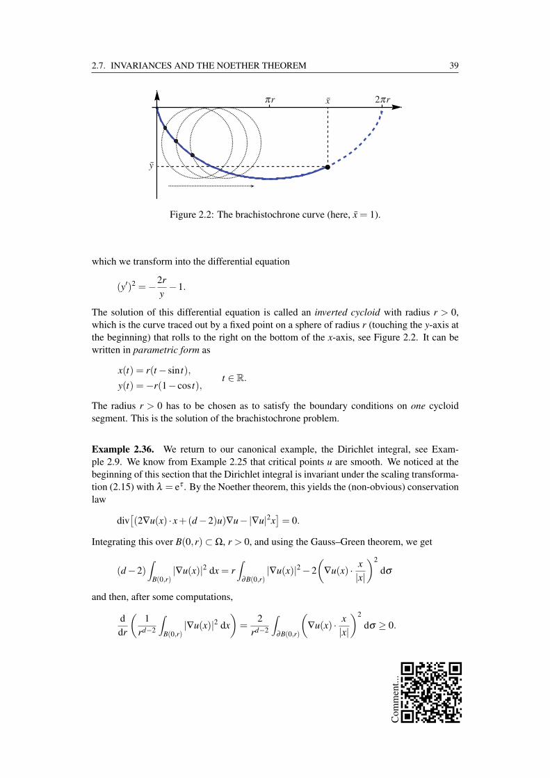
2.7. INVARIANCES AND THE NOETHER THEOREM 39
Figure 2.2: The brachistochrone curve (here, x = 1).
which we transform into the differential equation
(y′)2 =−2ry−1.
The solution of this differential equation is called an inverted cycloid with radius r > 0,which is the curve traced out by a fixed point on a sphere of radius r (touching the y-axis atthe beginning) that rolls to the right on the bottom of the x-axis, see Figure 2.2. It can bewritten in parametric form as
x(t) = r(t − sin t),
y(t) =−r(1− cos t),t ∈ R.
The radius r > 0 has to be chosen as to satisfy the boundary conditions on one cycloidsegment. This is the solution of the brachistochrone problem.
Example 2.36. We return to our canonical example, the Dirichlet integral, see Exam-ple 2.9. We know from Example 2.25 that critical points u are smooth. We noticed at thebeginning of this section that the Dirichlet integral is invariant under the scaling transforma-tion (2.15) with λ = eτ . By the Noether theorem, this yields the (non-obvious) conservationlaw
div[(2∇u(x) · x+(d −2)u)∇u−|∇u|2x
]= 0.
Integrating this over B(0,r)⊂ Ω, r > 0, and using the Gauss–Green theorem, we get
(d −2)∫
B(0,r)|∇u(x)|2 dx = r
∫∂B(0,r)
|∇u(x)|2 −2(
∇u(x) · x|x|
)2
dσ
and then, after some computations,
ddr
(1
rd−2
∫B(0,r)
|∇u(x)|2 dx)=
2rd−2
∫∂B(0,r)
(∇u(x) · x
|x|
)2
dσ ≥ 0.
Com
men
t...
40 CHAPTER 2. CONVEXITY
This monotonicity formula implies that
1rd−2
∫B(0,r)
|∇u(x)|2 dx is increasing in r > 0.
Any harmonic function (−∆u = 0) that is defined on all of Rd satisfies this monotonicityformula. For example, this allows us to draw the conclusion that if d ≥ 3, then u cannotbe compactly supported. The formula also shows that the growth around a singularity atzero (or anywhere else by translation) has to behave “more smoothly” than |x|−2 (in fact,we already know that solutions are C∞). While these are not particularly strong remarks,they serve to illustrate how Noether’s theorem restricts the candidates for solutions.
The last example exhibited a conservation law that was not obvious from the Euler–Lagrange equation. While in principle it could have been derived directly, the Noethertheorem gave us a systematic way to find this conservation law from an invariance.
2.8 Side constraints
In many minimization problems, the class of functions over which we minimize our func-tional may be restricted to include one or several side constraints. To establish existenceof a minimizer also in these cases, we first need to extend the Direct Method:
Theorem 2.37 (Direct Method with side constraint). Let X be a Banach space and letF ,G : X → R∪+∞. Assume the following:
(WH1) Weak Coercivity of F : For all Λ ∈ R, the sublevel set
u ∈ X : F [u]≤ Λ is sequentially weakly relatively compact,
that is, if F [u j] ≤ Λ for a sequence (u j) ⊂ X and some Λ ∈ R, then (u j) has aweakly convergent subsequence.
(WH2) Weak lower semicontinuity F : For all sequences (u j) ⊂ X with u j u (weakconvergence X) it holds that
F [u]≤ liminfj→∞
F [u j].
(WH3) Weak continuity of G : For all sequences (u j)⊂ X with u j x it holds that
G [u j]→ G [u].
Assume also that there exists at least one u0 ∈ X with G [u0] = 0. Then, the minimizationproblem
F [u]→ min over all u ∈ X with G [u] = α ∈ R,
has a solution.
Com
men
t...
2.8. SIDE CONSTRAINTS 41
Proof. The proof is almost exactly the same as the one for the standard Direct Method inTheorem 2.3. However, we need to select the u j for an infimizing sequence with G [u j] = α .Then, by (WH3), this property also holds for any weak limit u∗ of a subsequence of theu j’s.
A large class of side constraints can be treated using the following simple result:
Lemma 2.38. Let g : Ω×Rm → R be a Caratheodory integrand such that there existsM > 0 with
|g(x,v)| ≤ M(1+ |v|p), (x,v) ∈ Ω×Rm.
Then, G : W1,p(Ω;Rm)→ R defined through
G [u] :=∫
Ωg(x,u(x)) dx.
is weakly continuous.
Proof. Let u j u in W1,p, whereby after selecting a subsequence and employing theRellich–Kondrachov Theorem A.23 and Lemma A.4, u j → u in Lp (strongly) and almosteverywhere. By assumption we have
±g(x,v)+M(1+ |v|p)≥ 0.
Thus, applying Fatou’s Lemma separately to these two integrands, we get
liminfj→∞
(±G [u j]+
∫Ω
M(1+ |u j|p) dx)≥±G [u]+
∫Ω
M(1+ |u|p) dx.
Since ∥u j∥Lp → ∥u∥Lp , we can combine these two assertions to get G [u j] → G [u]. Sincethis holds for all subsequences, it also follows for our original sequence.
We will later see more complicated side constraints, in particular constraints involvingthe determinant of the gradient.
The following result is very important for the calculation of minimizers under sideconstraints. It effectively says that at a minimizer u∗ of F subject to the side constraintG [u∗] = 0, the derivatives of F and G have to be parallel, in analogy with the finite-dimensional situation.
Theorem 2.39 (Lagrange multipliers). Let f : Ω×Rm ×Rm×d →R, g : Ω×Rm →R beCaratheodory integrands and satisfy the growth bounds
| f (x,v,A)| ≤ M(1+ |v|p + |A|p),|g(x,v)| ≤ M(1+ |v|p), (x,v,A) ∈ Ω×Rm ×Rm×d,
Com
men
t...

42 CHAPTER 2. CONVEXITY
for some M > 0, 1 ≤ p < ∞, and let f ,g be continuously differentiable in v and A. Supposethat u∗ ∈ W1,p
g (Ω;Rm), where g ∈ W1−1/p,p(∂Ω;Rm), minimizes the functional
F [u] :=∫
Ωf (x,u(x),∇u(x)) dx, u ∈ W1,p
g (Ω;Rm),
under the side constraint
G [u] :=∫
Ωg(x,u(x)) dx = α ∈ R.
Assume furthermore that the consistency condition
δG [u∗][v] :=∫
ΩDvg(x,u∗(x)) · v(x) dx = 0 (2.20)
holds for at least one v ∈ W1,p0 (Ω;Rm). Then, there exists a Lagrange multiplier λ ∈ R
such that u∗ is a weak solution of the system of PDEs−div
[DA f (x,u,∇u)
]+Dv f (x,u,∇u) = λDvg(x,u) in Ω,
u = g on ∂Ω.(2.21)
Proof. The proof is structurally similar to its finite-dimensional analogue.Let u∗ ∈ W1,p
g (Ω;Rm) be a minimizer of F under the side constraint G [u∗] = 0. Fromthe consistency condition (2.20) we infer that there exists w ∈ W1,p
0 (Ω;Rm) such that
δG [u∗][w] =∫
ΩDvg(x,u∗) ·w dx = 1.
Now fix any variation v ∈ W1,p0 (Ω;Rm) and define for s, t ∈ R,
H(s, t) := G [u∗+ sv+ tw].
It is not difficult to see that H is continuously differentiable in both s and t (this uses thestrong continuity of the integral, see Theorem 2.31) and
∂sH(s, t) = δG [u∗+ sv+ tw][v],
∂tH(s, t) = δG [u∗+ sv+ tw][w].
Thus, by definition of w,
H(0,0) = α and ∂tH(0,0) = 1.
By the implicit function theorem, there exists a function τ : R→ R such that τ(0) = 0 and
H(s,τ(s)) = α for small |s|.
The chain rule yields for such s,
0 = ∂s[H(s,τ(s))] = ∂sH(s,τ(s))+∂tH(s,τ(s))τ ′(s),
Com
men
t...

2.8. SIDE CONSTRAINTS 43
whereby
τ ′(0) =−∂sH(0,0) =−∫
ΩDvg(x,u∗) · v dx. (2.22)
Now define for small |s| as above,
J(s) := F [u∗+ sv+ τ(s)w].
We have
G [u∗+ sv+ τ(s)w] = H(s,τ(s)) = α
and the continuously differentiable function J has a minimum at s = 0 by the minimiza-tion property of u∗. Thus, with the shorthand notations DA f = DA f (x,u∗,∇u∗) and Dv f =Dv f (x,u∗,∇u∗),
0 = J′(0) =∫
ΩDA f : (∇v+ τ ′(0)∇w)+Dv f · (v+ τ ′(0)w) dx.
Rearranging and using (2.22), we get∫Ω
DA f : ∇v+Dv f · v dx =−τ ′(0)∫
ΩDA f : ∇w+Dv f ·w dx
= λ∫
ΩDvg(x,u∗) · v dx, (2.23)
where we have defined
λ :=∫
ΩDA f : ∇w+Dv f ·w dx.
Since (2.23) shows that u∗ is a weak solution of (2.21), the proof is finished.
Example 2.40 (Stationary Schrodinger equation). When looking for ground states inquantum mechanics as in Section 1.3, we have to minimize
E [Ψ] :=∫RN
h2
2µ|∇Ψ|2 + 1
2V (x)|Ψ|2 dx
over all Ψ ∈ W1,2(RN ;C) under the side constraint
∥Ψ∥L2 = 1.
From Theorem 2.37 in conjunction with Lemma 2.38 (slightly extended to also apply tothe whole space Ω = RN) we see that this problem always has at least one solution. Theo-rem 2.39 (likewise extended) yields that this Ψ satisfies[
−h2
2µ∆ +V (x)
]Ψ(x) = EΨ(x), x ∈ Ω,
for some Lagrange multiplier E ∈ R, which is precisely the stationary Schrodinger equa-tion. One can also show that E > 0 is the smallest eigenvalue of the operator Ψ 7→ [−h2
2µ ∆ +
V (x)]Ψ.
Com
men
t...

44 CHAPTER 2. CONVEXITY
Notes and historical remarks
For the u-dependent variational integrals, the growth in the u-variable can be improved upto q-growth, where q < p/(p−d) (the Sobolev embedding exponent for W1,p). Moreover,we can work with the more general growth bounds | f (x,v,A)| ≤ M(g(x)+ |v|q+ |A|p), withg ∈ L1(Ω; [0,∞)) and q < p/(p − d). For reasons of simplicity, we have omitted thesegeneralization here.
The Fundamental Lemma of calculus of variations 2.21 is due to Du Bois-Raymond andis sometimes named after him.
Difference quotients were already considered by Newton, their application to regular-ity theory is due to Nirenberg in the 1940s and 1950s. Many of the fundamental resultsof regularity theory (albeit in a non-variational context) can be found in [48]. The bookby Giusti [49] contains theory relevant for variational questions. A nice framework forSchauder estimates is [98]. De Giorgi’s 1968 counterexample is from [32].
The Lavrentiev phenomenon was discovered in [68], our Example 2.32 is due to BasilioMania [70]. Tonelli’s Regularity Theorem [114] gives regularity for some integral function-als with superlinear growth; also see [52,53] for some recent developments in this direction.
Noether’s theorem has many ramifications and can be put into a very general form inHamiltonian systems and Lie-group theory. The idea is to study groups of symmetries andtheir actions. For an introduction into this diverse field see [93].
Example 2.36 about the monotonicity formula is from [42].Side constraints can also take the form of inequalities, which is often the case in Opti-
mization Theory or Mathematical Programming. This leads to Karush–Kuhn–Tucker con-ditions or obstacle problems.
A recent, very accesible introduction to the regularity for variational problems is in [13],also see the entertaining survey [77].
Com
men
t...
Chapter 3
Quasiconvexity
We saw in the last chapter that convexity of the integrand implies lower semicontinuity forintegral functionals. Moreover, we also mentioned in Proposition 2.11 that in the scalar cased = 1 or m = 1 convexity is also necessary for weak lower semicontinuity. In the vectorialcase (d,m> 1), however, it turns out that one can find weakly lower semicontinuous integralfunctionals whose integrand is non-convex. The following is the most prominent one: Letp ≥ d (Ω ⊂ Rd a bounded Lipschitz domain as usual) and define
F [u] :=∫
Ωdet∇u(x) dx, u ∈ W1,p
0 (Ω;Rd).
Then, we can argue using the Stokes theorem (this can also be computed in a more elemen-tary way, see Lemma 3.8 below):
F [u] =∫
Ωdet∇u dx =
∫Ω
du1 ∧·· ·∧dud =∫
∂Ωu1 ∧du2 ∧·· ·∧dud = 0,
because u ∈ W1,d0 (Ω;Rd) is zero near the boundary ∂Ω. Thus, F is in fact constant on
W1,p0 (Ω;Rd), hence trivially weakly lower semicontinuous. However, the determinant func-
tion is far from being convex if d ≥ 2; for instance we can easily convex-combine a matrixwith positive determinant from two singular ones. But we can also find examples not in-volving singular matrices: For
A :=(−1 −22 1
), B :=
(1 −22 −1
),
12
A+12
B =
(0 −22 0
),
we have det A = detB = 3, but det(A/2+B/2) = 4.Furthermore, convexity of the integrand is not compatible with one of the most funda-
mental principles of continuum mechanics: Assume that our integrand f = f (A) is frame-indifferent, that is,
f (RA) = f (A) for all A ∈ Rd×d , R ∈ SO(d),
Com
men
t...
46 CHAPTER 3. QUASICONVEXITY
where SO(d) is the set of (d × d)-orthogonal matrices with determinant 1, i.e. rotations.Furthermore, assume that every purely compressive or purely expansive deformation costsenergy, i.e.
f (α Id)> f (Id) for all α = 1, (3.1)
which is very reasonable in applications. Then, f cannot be convex: Let us for simplicityassume d = 2. Set, for a fixed γ ∈ (0,2π),
R :=(
cosγ −sinγsinγ cosγ
)∈ SO(2).
Then, if f was convex, for M := (R+RT )/2 = (cosγ) Id we would get
f ((cosγ) Id) = f (M)≤ 12(
f (R)+ f (RT ))= f (Id),
contradicting (3.1). Sharper arguments are available, but the essential conclusion is thesame: convexity is not suitable for many variational problems originating from continuummechanics.
3.1 Quasiconvexity
We are now ready to replace convexity with a more general notion, which has become oneof the cornerstones of the modern calculus of variations. This is the notion of quasicon-vexity, introduced by Charles B. Morrey in the 1950s: A locally bounded Borel-measurablefunction h : Rm×d → R is called quasiconvex if
h(A)≤ −∫
B(0,1)h(A+∇ψ(z)) dz (3.2)
for all A ∈ Rm×d and all ψ ∈ W1,∞0 (B(0,1);Rm). Here, −
∫B(0,1) := ω−1
d∫
B(0,1), where B(0,1)is the unit ball in Rd and its volume is ωd := |B(0,1)|.
Let us give a physical interpretation of quasiconvexity: Let d = m = 3 and assume that
F [y] :=∫
B(0,1)h(∇y(x)) dx, y ∈ W1,∞(B(0,1);R3),
models the physical energy of an elastically deformed body, whose deformation from thereference configuration is given as y : Ω = B(0,1)→ R3 (see Section 1.4 for more detailson this modeling). A special class of deformations are the affine ones, a(x) = y0 +Ax forsome y0 ∈ R3, A ∈ R3×3. Then, quasiconvexity of f entails that
F [a] =∫
B(0,1)h(A) dx ≤
∫B(0,1)
h(A+∇ψ(z)) dz = F [a+ψ]
for all ψ ∈ W1,∞0 (B(0,1);R3). This means that the affine deformation a is always ener-
getically favorable over the internally distorted deformation a + ψ; this is very often a
Com
men
t...
3.1. QUASICONVEXITY 47
reasonable assumption for real materials. This argument also holds on any other domain byLemma 3.2 below.
To justify its name, we also need to convince ourselves that quasiconvexity is indeed anotion of convexity: For A∈Rm×d and V ∈L1(B(0,1);Rm×d) with
∫B(0,1)V (x) dx= 0 define
the probability measure µ ∈ M1(Rm×d) via its action as follows (recall that M (Rm×d) ∼=C0(Rm×d)∗ by the Riesz Representation Theorem A.12):⟨
h,µ⟩
:= −∫
B(0,1)h(A+V (x)) dx for h ∈ C0(Rm×d).
This µ is easily seen to be an element of the dual space to C0(Rm×d), and in fact µ is aprobability measure: For the boundedness we observe |⟨h,µ⟩| ≤ ∥h∥∞, whereas the positiv-ity ⟨h,µ⟩ ≥ 0 for h ≥ 0 and the normalization ⟨1,µ⟩= 1 follow at once. The barycenter [µ]of µ is
[µ] := ⟨id,µ⟩= A+ −∫
B(0,1)V (x) dx = A.
Therefore, if h is convex, we get from then Jensen inequality, Lemma A.11,
h(A) = h([µ])≤⟨h,µ⟩= −∫
B(0,1)h(A+V (x)) dx.
In particular, (3.2) holds if we set V (x) := ∇ψ(x) for any ψ ∈ W1,∞0 (B(0,1);Rm). Thus, we
have shown:
Proposition 3.1. All convex functions h : Rm×d → R are quasiconvex.
Some basic properties of quasiconvexity are collected in the following lemma.
Lemma 3.2. (i) In the definition of quasiconvexity we can replace the domain B(0,1)by any bounded Lipschitz domain Ω′ ⊂ Rd .
(ii) If h has p-growth, i.e. |h(A)| ≤ M(1+ |A|p) for some 1 ≤ p < ∞, M > 0, then in thedefinition of quasiconvexity we can replace testing with all ψ ∈ W1,∞
0 by testing withall ψ ∈ W1,p
0 .
Proof. To see the first statement, we will prove the following claim: If ψ ∈ W1,p(Ω;Rm),where Ω ⊂ Rd is a bounded Lipschitz domain, satisfies ψ(x)|∂Ω = Ax for some A ∈ Rm×d
(in the sense of trace), then there exists ψ ∈ W1,p(Ω′;Rm) with ψ(x)|∂Ω′ = Ax and, if oneof the following integrals exists and is finite, then
−∫
Ωh(∇ψ) dx = −
∫Ω′
h(∇ψ) dy for all measurable h : Rm×d → R. (3.3)
In particular, ∥∇ψ∥Lp = ∥∇ψ∥Lp . Clearly, this implies that the definition of quasiconvexityis independent of the domain.
Com
men
t...
48 CHAPTER 3. QUASICONVEXITY
To see (3.3), take a Vitali cover of Ω′ with re-scaled versions of Ω, see Theorem A.10,
Ω′ = Z ∪N∪
k=1
Ω(ak,rk), |Z|= 0,
with ak ∈ Ω, rk > 0, Ω(ak,rk) := ak + rkΩ, where k = 1, . . . ,N ∈ N. Then let
ψ(y) :=
rkψ(
y−ak
rk
)+Aak if y ∈ Ω(ak,rk),
0 otherwise,y ∈ Ω′.
It holds that ψ ∈ W1,∞(Ω′;Rm). We compute for any measurable h : Rm×d → R,∫Ω′
h(∇ψ) dy = ∑k
∫Ω(ak,rk)
h(
∇ψ(
y−ak
rk
))dy
= ∑k
rdk
∫Ω
h(∇ψ) dx
=|Ω′||Ω|
∫Ω
h(∇ψ) dx
since ∑k rdk = |Ω′|/|Ω|. This shows (3.3).
The second assertion follows since W1,∞0 (B(0,1);Rm) is dense in W1,p
0 (B(0,1);Rm) andunder a p-growth assumption, the integral functional
ψ 7→ −∫
Ωh(∇ψ) dx, ψ ∈ W1,p
0 (B(0,1);Rm),
is well-defined and continuous, the latter for example by Pratt’s Theorem A.6, see the proofof Theorem 2.31 for a similar argument.
An even weaker notion of convexity is the following one: A locally bounded Borel-measurable function h : Rm×d → R is called rank-one convex if it is convex along anyrank-one line, that is,
h(θA+(1−θ)B
)≤ θh(A)+(1−θ)h(B)
for all A,B ∈ Rm×d with rank(A−B) ≤ 1 and all θ ∈ (0,1). In this context, recall that amatrix M ∈ Rm×d has rank one if and only if M = a⊗b = abT for some a ∈ Rm, b ∈ Rd .
Proposition 3.3. If h : Rm×d → R is quasiconvex, then it is rank-one convex.
Proof of Proposition 3.3. Let A,B ∈ Rm×d with B−A = a⊗n for a ∈ Rm and n ∈ Rd with|n|= 1. Denote by Qn a unit cube (|Qn|= 1) centered at the origin and with one face normaln. By Lemma 3.2 we can require h to satisfy
h(M)≤ −∫
Qn
h(∇ψ(z)) dz (3.4)
Com
men
t...
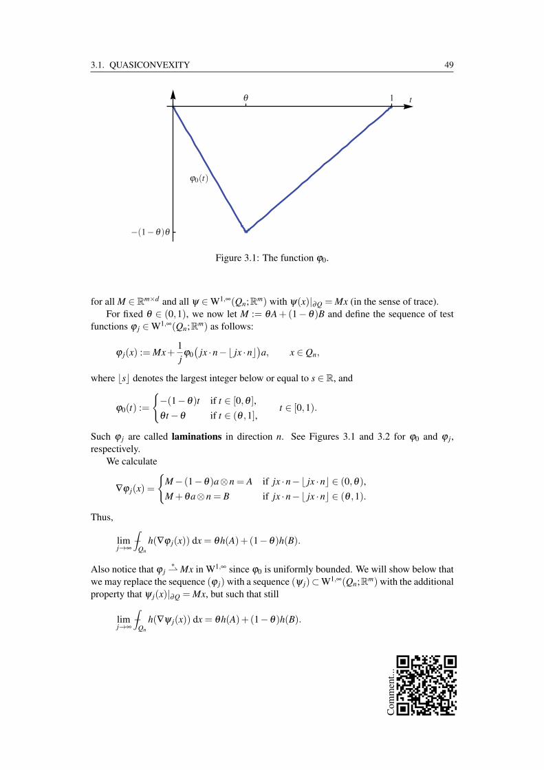
3.1. QUASICONVEXITY 49
Figure 3.1: The function φ0.
for all M ∈ Rm×d and all ψ ∈ W1,∞(Qn;Rm) with ψ(x)|∂Q = Mx (in the sense of trace).For fixed θ ∈ (0,1), we now let M := θA+(1− θ)B and define the sequence of test
functions φ j ∈ W1,∞(Qn;Rm) as follows:
φ j(x) := Mx+1jφ0(
jx ·n−⌊ jx ·n⌋)a, x ∈ Qn,
where ⌊s⌋ denotes the largest integer below or equal to s ∈ R, and
φ0(t) :=
−(1−θ)t if t ∈ [0,θ ],θ t −θ if t ∈ (θ ,1],
t ∈ [0,1).
Such φ j are called laminations in direction n. See Figures 3.1 and 3.2 for φ0 and φ j,respectively.
We calculate
∇φ j(x) =
M− (1−θ)a⊗n = A if jx ·n−⌊ jx ·n⌋ ∈ (0,θ),M+θa⊗n = B if jx ·n−⌊ jx ·n⌋ ∈ (θ ,1).
Thus,
limj→∞
−∫
Qn
h(∇φ j(x)) dx = θh(A)+(1−θ)h(B).
Also notice that φ j∗ Mx in W1,∞ since φ0 is uniformly bounded. We will show below that
we may replace the sequence (φ j) with a sequence (ψ j)⊂W1,∞(Qn;Rm) with the additionalproperty that ψ j(x)|∂Q = Mx, but such that still
limj→∞
−∫
Qn
h(∇ψ j(x)) dx = θh(A)+(1−θ)h(B).
Com
men
t...

50 CHAPTER 3. QUASICONVEXITY
Figure 3.2: The laminate φ j.
Combining this with (3.4) allows us to conclude
h(θA+(1−θ)B
)≤ θh(A)+(1−θ)h(B)
and h is indeed rank-one convex.It remains to construct the sequence (ψ j) from (φ j), for which we employ a standard
cut-off construction: Take a sequence (ρ j) ⊂ C∞c (Qn; [0,1]) of cut-off functions such that
for G j :=
x ∈ Ω : ρ j(x) = 1
it holds that |Qn \G j| → 0 as j → ∞. Set
ψ j,k(x) := ρ jφk(x)+(1−ρ j)Mx, x ∈ Ω,
which lies in W1,∞(Qn;Rm) and satisfies ψ j,k(x) = Mx near ∂Qn. Also,
∇ψ j,k = ρ j∇φk +(1−ρ j)M+(φk −a)⊗∇ρ j.
Since W1,∞(Qn;Rm) embeds compactly into L∞(Qn;Rm) by the Rellich-Kondrachov theo-rem (or the classical Arzela–Ascoli theorem), we have φk → Mx uniformly. Thus, in
∥∇ψ j,k∥L∞ ≤ ∥∇φk∥L∞ + |M|+∥(φk −a)⊗∇ρ j∥L∞
the last term vanishes as k → ∞. As the ∇φk furthermore are uniformly L∞-bounded, wecan for every j ∈N choose k( j) ∈N such that ∥∇ψ j,k( j)∥L∞ is bounded by a constant that isindependent of j. Then, as h is assumed to be locally bounded, this implies that there existsC > 0 (again independent of j) with
∥h(∇φ j)∥L∞ +∥h(∇ψ j,k( j))∥L∞ ≤C.
Com
men
t...

3.1. QUASICONVEXITY 51
Hence, for ψ j := ψ j,k( j), we may estimate
limj→∞
∫Qn
|h(∇φ j)−h(∇ψ j)| dx = limj→∞
∫Qn\G j
|h(∇φ j)|+ |h(∇ψ j,k( j))| dx
≤ limj→∞
C|Qn \G j|= 0.
This shows that above we may replace (φ j) by (ψ j).
Since for d = 1 or m = 1, rank-one convexity obviously is equivalent to convexity, wehave for the scalar case:
Corollary 3.4. If h : Rm×d → R is quasiconvex and d = 1 or m = 1, then h is convex.
However, quasiconvexity is weaker than classical convexity if d,m≥ 2. The determinantfunction and, more generally, minors are quasiconvex, as will be proved in the next section,but these minors (except for (1× 1)-minors) are not convex. The following is a standardexample of a quasiconvex function.
Example 3.5 (Alibert–Dacorogna–Marcellini). For d = m = 2 and γ ∈ R define
hγ(A) := |A|2(|A|2 −2γ det A
), A ∈ R2×2.
For this function it is known that
• hγ is convex if and only if |γ| ≤ 2√
23
≈ 0.94,
• hγ is rank-one convex if and only if |γ| ≤ 2√3≈ 1.15,
• hγ is quasiconvex if and only if |γ| ≤ γQC for some γQC ∈(
1,2√3
].
It is currently unknown whether γQC = 2/√
3. We do not prove these statements here, seeSection 5.3.8 in [29] for the details.
We end this section with the following regularity theorem for rank-one convex (andhence also for quasiconvex) functions:
Proposition 3.6. If h : Rm×d → R is rank-one convex, then it is locally Lipschitz continu-ous. If additionally h has p-growth, then
|h(A)−h(B)| ≤C(1+ |A|p−1 + |B|p−1)|A−B| for all A,B ∈ Rm×d (3.5)
and a dimensional constant C = C(d,m). In particular, a rank-one convex h with lineargrowth is (globally) Lipschitz continuous.
Com
men
t...

52 CHAPTER 3. QUASICONVEXITY
Proof. For any A0 ∈ Rm×d and r > 0, we will prove the stronger quantitative bound
lip(h;B(A0,r))≤√
min(d,m) · osc(h;B(A0,6r))3r
, (3.6)
where
lip(h;B(A0,r)) := supA,B∈B(A0,r)
|h(A)−h(B)||A−B|
is the Lipschitz constant of h on the ball B(A0,r)⊂ Rm×d , and
osc(h;B(A0,r)) := supA,B∈B(A0,r)
|h(A)−h(B)|
is the oscillation of h on B(A0,r). By the local boundedness of h, which is part of ourdefinition of rank-one convexity, the oscillation is bounded on every ball. Thus the Lipschitzconstant is locally finite.
To show (3.6), let A,B ∈ B(x0,r) and assume first that rank(A−B)≤ 1. Define the pointC ∈ Rm×d as the intersection of ∂B(A0,2r) with the ray starting at B and going through A.Then, because h is convex along this ray,
|h(A)−h(B)||A−B|
≤ |h(C)−h(B)||C−B|
≤ osc(h;B(A0,2r))r
=: α(2r). (3.7)
For general A,B ∈ B(A0,r), use the (real) singular value decomposition to write
B−A =min(d,m)
∑i=1
σiP(ei ⊗ ei)QT ,
where σi ≥ 0 is the i’th singular value, and P ∈ Rm×m, Q ∈ Rd×d are orthogonal matrices.Set
Ak := A+k−1
∑i=1
σiP(ei ⊗ ei)QT , k = 1, . . . ,min(d,m)+1,
for which we have A1 = A, Amin(d,m)+1 = B. We estimate (recall that we are employing the
Frobenius norm |M| :=√
∑ j,k(Mjk )
2 =√
∑i σi(M)2)
|Ak −A0| ≤ |A−A0|+
√k−1
∑i=1
σ 2i ≤ |A−A0|+ |B−A|< 3r
and
min(d,m)
∑k=1
|Ak −Ak+1|2 =min(d,m)
∑k=1
σ2i = |A−B|2.
Com
men
t...

3.2. NULL-LAGRANGIANS 53
Applying (3.7) to Ak,Ak+1 ∈ B(A0,3r), k = 1, . . . ,min(d,m), we get
|h(A)−h(B)| ≤min(d,m)
∑k=1
|h(Ak)−h(Ak+1)|
≤ α(6r)min(d,m)
∑k=1
|Ak −Ak+1|
≤ α(6r)√
min(d,m) ·
[min(d,m)
∑k=1
|Ak −Ak+1|2]1/2
= α(6r)√
min(d,m) · |A−B|.
This yields (3.6).If we additionally assume that h has p-growth, then
osc(h;B(0,r))≤C(1+ rp),
and so, with r := max|A|, |B|, the estimate (3.5) follows from (3.6).
Remark 3.7. An improved argument (see Lemma 2.2 in [11]), where one orders the sin-gular values in a favorable way, allows to establish the better estimate
lip(h;B(A0,r))≤√
min(d,m) · osc(h;B(A0,2r))r
.
3.2 Null-Lagrangians
The determinant is quasiconvex, but it is only one representative of a larger class of canon-ical examples of quasiconvex, but not convex, functions: In this section, we will investigatethe properties of minors (subdeterminants) as integrands. Let for r ∈ 1,2, . . . ,min(d,m),
I ∈ P(m,r) :=(i1, i2, . . . , ir) ∈ 1, . . . ,mr : i1 < i2 < · · ·< ir
and J ∈ P(d,r) be ordered multi-indices. Then, a (r× r)-minor M : Rm×d → R is a func-tion of the form
M(A) = MIJ(A) := det
(AI
J),
where AIJ is the (square) matrix consisting of the I-rows and J-columns of A. The number
r ∈ 1, . . . ,min(d,m) is called the rank of the minor M.The first result shows that all minors are null-Lagrangians, which by definition is the
class of integrands h : Rm×d such that∫
Ω h(∇u) dx only depends on the boundary values ofu.
Lemma 3.8. Let M : Rm×d → R be a (r × r)-minor, r ∈ 1, . . . ,min(d,m). If u,v ∈W1,p(Ω;Rm), p ≥ r, with u− v ∈ W1,p
0 (Ω;Rm), then∫Ω
M(∇u) dx =∫
ΩM(∇v) dx.
Com
men
t...
54 CHAPTER 3. QUASICONVEXITY
Proof. In all of the following, we will assume that u,v are smooth and supp(u− v) ⋐ Ω,which can be achieved by approximation and a cut-off procedure, see Theorem A.24. Wealso need that taking the minor M of the gradient commutes with strong convergence, i.e. thestrong continuity of u 7→ M(∇u) in W1,p for p ≥ r; this follows by Hadamard’s inequality|M(A)| ≤ |A|r and Pratt’s Theorem A.6 (see the proof of Lemma 2.38).
All first-order minors are just the entries of ∇u,∇v and the result follows from∫Ω
∇u dx =∫
∂Ωu ·n dσ =
∫∂Ω
v ·n dσ =∫
Ω∇v dx
since supp(u− v)⋐Ω.For higher-order minors, the crucial observation is that minors of gradients can be writ-
ten as divergences, which we will establish below. So, if M(∇u) = divG(u,∇u), then, sincesupp(u− v)⋐Ω,∫
ΩM(∇u) dx =
∫∂Ω
G(u,∇u) ·n dσ =∫
∂ΩG(v,∇v) ·n dσ =
∫Ω
M(∇v) dx
and the result follows.We first consider the physically most relevant cases d = m ∈ 2,3.For d = m = 2 and u = (u1,u2)T , the only second-order minor is the Jacobian determi-
nant and we easily see from the fact that second derivatives of smooth functions commutethat
det∇u = ∂1u1∂2u2 −∂2u1∂1u2
= ∂1(u1∂2u2)−∂2(u1∂1u2)
= div(u1∂2u2,−u1∂1u2).
For d = m = 3, consider a second-order minor M¬k¬l (A), i.e. the determinant of A after
deleting the k’th row and l’th column. Then, analogously to the situation in dimension two,we get, using cyclic indices k, l ∈ 1,2,3,
M¬k¬l (∇u) = (−1)k+l[∂l+1uk+1∂l+2uk+2 −∂l+2uk+1∂l+1uk+2]
= (−1)k+l[∂l+1(uk+1∂l+2uk+2)−∂l+2(uk+1∂l+1uk+2)]. (3.8)
For the three-dimensional Jacobian determinant, we will show
det∇u =3
∑l=1
∂l(u1(cof∇u)1
l), (3.9)
where we recall that (cofA)kl = (−1)k+lM¬k
¬l (A). To see this, use the Cramer formula(det A)I = A(cofA)T , which holds for any matrix A ∈ Rn×n, to get
det∇u =3
∑l=1
∂lu1 · (cof∇u)1l .
Com
men
t...

3.2. NULL-LAGRANGIANS 55
Then, our formula (3.9) follows from the Piola identity
divcof∇u = 0, (3.10)
which can be verified directly from the expression (3.8) for M¬k¬l (∇u). Hence, (3.9) holds.
For general dimensions d,m we use the notation of differential geometry to tame the multi-linear algebra involved in the proof. So, let M be a (r× r)-minor. Reordering x1, . . . ,xd andu1, . . . ,um, we can assume without loss of generality that M is a principal minor, i.e. M isthe determinant of the top-left (r× r)-submatrix. Then,
M(∇u)dx1 ∧·· ·∧dxd = du1 ∧·· ·∧dur ∧dxr+1 ∧·· ·∧dxd
= d(u1 ∧du2 ∧·· ·∧dur ∧dxr+1 ∧·· ·∧dxd).
Thus, the general Stokes theorem gives∫Ω
M(∇u)dx1 ∧·· ·∧dxd =∫
Ωd(u1 ∧du2 ∧·· ·∧dur ∧dxr+1 ∧·· ·∧dxd)
=∫
∂Ωu1 ∧du2 ∧·· ·∧dur ∧dxr+1 ∧·· ·∧dxd .
Therefore,∫
Ω M(∇u)dx1 ∧·· ·∧dxd only depends on the values of u around ∂Ω.
Consequently, we also have:
Corollary 3.9. All (r× r)-minors M : Rm×d →R are quasiaffine, that is, both M and −Mare quasiconvex.
We will later use this property to define a large and useful class of quasiconvex func-tions, namely the polyconvex ones; this is the topic of the next chapter.
Further, minors enjoy a surprising continuity property:
Lemma 3.10 (Weak continuity of minors). Let M : Rm×d → R be an (r× r)-minor, r ∈1, . . . ,min(d,m), and (u j)⊂ W1,p(Ω;Rm) where r < p ≤ ∞. If
u j u in W1,p (or u j∗ u in W1,∞).
then
M(∇u j) M(∇u) in Lp/r (or M(∇u j)∗ M(∇u) in W1,∞).
Proof. For d = m ∈ 2,3, we use the special structure of minors as divergences, as ex-hibited in the proof of Lemma 3.8. For a (2× 2)-minor M¬k
¬l in three dimensions (that is,deleting the k’th row and l’th column; in two dimensions there is only one (2× 2)-minor,the determinant, but we still use the same notation), we rely on (3.8) to observe that withcyclic indices k, l ∈ 1,2,3,∫
ΩM¬k
¬l (∇u j)ψ dx =−(−1)k+l∫
Ω(uk+1
j ∂l+2uk+2j )∂l+1ψ − (uk+1
j ∂l+1uk+2j )∂l+2ψ dx
Com
men
t...
56 CHAPTER 3. QUASICONVEXITY
for all ψ ∈ C∞c (Ω) and then by density also for all ψ ∈ Lp/r(Ω)∗ ∼= Lp/(p−r)(Ω). Since
u j u in W1,p, we have u j → u strongly in Lp. The above expression consists of productsof one Lp-weakly and one Lp-strongly convergent factor as well as a uniformly boundedfunction under the integral. Hence the integral is weakly continuous and as j →∞ convergesto ∫
ΩM¬k
¬l (∇u)ψ dx.
This finishes the proof for d = m = 2.For d = m = 3, we additionally need to consider the determinant. However, as a conse-
quence of the two-dimensional reasoning, cof∇u j cof∇u in Lp/2. Then, (3.9) implies
∫Ω
det∇u j ψ dx =−3
∑l=1
∫Ω
[u1
j(cof∇u j)1l]∂lψ dx
and by a similar reasoning as above, this converges to
−3
∑l=1
∫Ω
[u1(cof∇u)1
l]∂lψ dx =
∫Ω
det∇uψ dx.
In the general case, one proceeds by induction.
It can also be shown that any quasiaffine function can be written as an affine functionof all the minors of the argument. This characterization of quasiaffine functions is due toBall [4], a different proof (also including further characterizing statements) can be found inTheorem 5.20 of [29].
3.3 Young measures
We now introduce a very versatile tool for the study of minimization problems, the Youngmeasure, named after its inventor Laurence Chisholm Young. In this chapter, we will onlyuse it as a device to organize the proof of lower semicontinuity for quasiconvex integralfunctions, see Theorems 3.28, 3.33, but later it will also be important as an object in its ownright.
Let us motivate this device through the following central question: Assume that wehave a weakly convergent sequence v j v in L2(Ω), where Ω ⊂Rd is a bounded Lipschitzdomain, and an integral functional
F [v] :=∫
Ωf (x,v(x)) dx
with f : Ω×R→ R continuous and bounded, say. Then, we may want to know the limit ofF [v j] as j → ∞, for instance if (v j) is a minimizing sequence. In fact, this will be corner-stone of the proof of weak lower semicontinuity for integral functionals with quasiconvexintegrands.
Com
men
t...

3.3. YOUNG MEASURES 57
Equivalently, we could ask for the weak* limit in L∞ of the sequence of compoundfunctions g j(x) := f (x,v j(x)). It is easy to see that the weak* limit in general is not equalto x 7→ f (x,v(x)). For example, in Ω = (0,1), consider the sequence
v j(x) :=
a if jx−⌊ jx⌋ ≤ θ ,b otherwise,
x ∈ Ω,
where a,b ∈ R, θ ∈ (0,1), and ⌊s⌋ is the largest integer below or equal to s ∈ R. Then, iff (x,a) = α ∈ R and f (x,b) = β ∈ R (and smooth and bounded elsewhere), we see v j
∗
θa+(1−θ)b and
f (x,v j(x))∗ h(x) = θα +(1−θ)β .
The right-hand side, however, is not necessarily f (x,θa+ (1− θ)b). Instead, we couldwrite
h(x) =⟨
f (x, q),νx⟩=∫
f (x,v) dνx(v)
with a x-parametrized family of probability measures νx ∈ M1(R), namely
νx = θδα +(1−θ)δβ , x ∈ (0,1).
This family (νx)x∈Ω is the “Young measure generated by the sequence (v j)”.We start with the fundamental theorem of Young measure theory:
Theorem 3.11 (Young 1937). Let (Vj) ⊂ Lp(Ω;RN) be a bounded sequence, where 1 ≤p ≤ ∞. Then, there exists a subsequence (not relabeled) and a family (νx)x∈Ω ⊂ M1(RN)of probability measures, called the (Lp-)Young measure generated by the sequence (Vj),such that the following assertions are true:
(i) The family (νx) is weakly* measurable, i.e., for all Caratheodory integrands f : Ω×RN → R, the compound function
x 7→⟨
f (x, q),νx⟩=∫
f (x,A) dνx(A), x ∈ Ω,
is Lebesgue-measurable.
(ii) If 1 ≤ p < ∞, it holds that⟨⟨| q|p,ν⟩⟩ :=
∫Ω
∫|A|p dνx(A) dx < ∞,
or, if p = ∞, there exists a compact set K ⊂ RN such that
suppνx ⊂ K for a.e. x ∈ Ω.
Com
men
t...

58 CHAPTER 3. QUASICONVEXITY
(iii) For all Caratheodory integrands f : Ω×RN → R such that the family ( f (x,Vj(x))) j
is uniformly L1-bounded and equiintegrable, it holds that
f (x,Vj(x))
(x 7→
∫f (x,A) dνx(A)
)in L1(Ω). (3.11)
For parametrized measures ν = (νx)x∈Ω that satisfy (i) and (ii) above, we write ν =(νx) ∈ Yp(Ω;RN), the latter being called the set of Lp-Young measures. In symbols weexpress the generation of a Young measure ν by as sequence (Vj) as
VjY→ ν .
Furthermore, the convergence (3.11) can equivalently be expressed as (absorb a test functionfor weak convergence into f )∫
Ωf (x,Vj(x)) dx →
∫Ω
∫f (x,A) dνx(A) dx =:
⟨⟨f ,ν⟩⟩.
We call⟨⟨
f ,ν⟩⟩
the duality pairing between f and ν . In this context, recall from theDunford–Pettis Theorem A.17 that ( f (x,Vj(x))) j is equiintegrable if and only it is weaklyrelatively compact in L1(Ω).
Remark 3.12. Some assumptions in the fundamental theorem can be weakened: For theexistence of a Young measure, we only need to require
limK↑∞
sup j ||Vj| ≥ K|= 0,
which for example follows from sup j∫
Ω |Vj|r dx < ∞ for some r > 0. Of course, in thiscase (ii) needs to be suitably adapted.
Proof. We associate with each Vj an elementary Young measure δ [Vj] ∈ Yp(Ω;RN) asfollows:
(δ [Vj])x := δV j(x) for a.e. x ∈ Ω. (3.12)
Below we will show the following Young measure compactness principle:
Lemma 3.13. Let 1 ≤ p ≤ ∞ and let (ν( j)) j ⊂ Yp(Ω;RN) be a sequence of Lp-Youngmeasures such that, if 1 ≤ p < ∞,
sup j⟨⟨| q|p,ν( j)⟩⟩= sup j
∫Ω
∫|A|p dν( j)
x (A) dx < ∞ (3.13)
or, if p = ∞, suppν( j)x ⊂ K for all j ∈ N, almost every x ∈ Ω, and a compact set K ⊂ Rm×d .
Then, there exists a subsequence of the (ν j) (not relabeled) and ν ∈ Yp(Ω;RN) such that
limj→∞
⟨⟨f ,ν( j)⟩⟩= ⟨⟨ f ,ν
⟩⟩(3.14)
Com
men
t...

3.3. YOUNG MEASURES 59
for all Caratheodory f : Ω×RN →R for which the sequence of functions x 7→ ⟨ f (x, q),ν( j)x ⟩
is uniformly L1-bounded and the equiintegrability condition
sup j⟨⟨
f (x,A)1| f (x,A)|≥m,ν( j)⟩⟩→ 0 as m → ∞. (3.15)
holds. Moreover,⟨⟨| q|p,ν⟩⟩≤ liminf
j→∞
⟨⟨| q|p,ν( j)⟩⟩.
In the theorem, our assumption of Lp-boundedness of (Vj) corresponds to (3.13), so (i)–(III) follow immediately from the compactness principle applied to our sequence (δ [Vj]) j
of elementary Young measures from (3.12) above once we realize that for the sequence ofYoung measures (δ [Vj]) j the condition (3.15) corresponds precisely to the equiintegrabilityof ( f (x,Vj(x))) j.
Proof of Lemma 3.13. Define the measures
µ( j) := L dx Ω⊗ν( j)
x ,
which is just a shorthand notation for the Radon measures µ( j) ∈ M (Ω×RN) ∼= C0(Ω×RN)∗ defined through their action⟨
f ,µ( j)⟩= ∫Ω
∫f (x,A) dν( j)
x (A) dx for all f ∈ C0(Ω×RN).
So, for the ν( j) = δ [Vj] from (3.12), we recover the familiar form⟨f ,µ( j)⟩= ∫
Ωf (x,Vj(x)) dx for all f ∈ C0(Ω×RN),
but in the compactness principle we might be in a more general situation.Clearly, every so-defined µ( j) is a positive measure and∣∣⟨ f ,µ( j)⟩∣∣≤ |Ω| · ∥ f∥∞,
whereby the (µ( j)) constitute a uniformly bounded sequence in the dual space C0(Ω×RN)∗.Thus, by the Sequential Banach–Alaoglu Theorem A.16, we can select a (non-relabeled)subsequence such that with a µ ∈ C0(Ω×RN)∗ it holds that⟨
f ,µ( j)⟩→ ⟨f ,µ⟩
for all f ∈ C0(Ω×RN). (3.16)
Next we will show that µ can be written as µ = L dx Ω⊗νx for a weakly* measurable
parametrized family ν = (νx)x∈Ω ⊂ M1(RN) of probability measures.
Theorem 3.14 (Disintegration). Let µ ∈ M (Ω×RN) be a finite Radon measure. Then,there exists a weakly* measurable family (νx)x∈Ω ⊂ M1(RN) of probability measures suchthat with κ(A) := µ(A×RN),
µ = κ(dx)⊗νx,
that is,∫f dµ =
∫Ω
∫f (x,A) dνx(A) dκ(x) for all f ∈ C0(Ω×RN).
Com
men
t...
60 CHAPTER 3. QUASICONVEXITY
A proof of this measure-theoretic result can be found in Theorem 2.28 of [1].In our situation, we have for f (x,v) := φ(x) with arbitrary φ ∈ C0(Ω) that
∫φ dµ = lim
j→∞
∫φ dµ( j) =
∫Ω
φ(x) dx,
and so κ = L d Ω. Hence, the disintegration theorem immediately yields the weak* mea-surability of (νx) and thus lim j→∞ ⟨⟨ f ,ν( j)⟩⟩=
⟨⟨f ,ν⟩⟩
for f ∈ C0(Ω×RN), which is (3.14).Next, we show (3.14) for the case of f merely Caratheodory and bounded and such that
there exists a compact set K ⊂ RN with supp f ⊂ Ω×K. We invoke the Scorza DragoniTheorem 2.5 to get an increasing sequence of compact sets Sk ⋐Ω (k ∈N) with |Ω\Sk| ↓ 0such that f |Sk×RN is continuous. Let fk ∈ C(Ω×RN) be an extension of f |Sk×RN to all ofΩ×RN with the property that the fk are uniformly bounded. Indeed, since K is boundedand | fk(x,A)| ≤ M(1+ |A|p), f is bounded and hence we may require uniform boundednessof the fk.
Now, since fk ∈ C0(Ω×RN), (3.16) implies
⟨fk(x, q),ν( j)
x⟩
⟨
fk(x, q),νx⟩
in L1 (as functions of x) as j → ∞.
Thus, we also get
⟨f (x, q),ν( j)
x⟩
⟨
f (x, q),νx⟩
in L1(Sk) (as functions of x) as j → ∞.
On the other hand,
∫Ω
∣∣⟨ f (x, q),ν( j)x⟩−1Sk
⟨f (x, q),ν( j)
x⟩∣∣ dx ≤
∫Ω\Sk
∣∣⟨ f (x, q),ν( j)x⟩∣∣ dx
and this converges to zero as k → ∞, uniformly in j, by the uniform boundedness of fk; thesame estimate holds with ν in place of ν( j). Therefore, we may conclude
⟨f (x, q),ν( j)
x⟩
⟨
f (x, q),νx⟩
in L1(Ω) (as functions of x) as j → ∞,
which directly implies (3.14) (for f with supp f ⊂ Ω×K).Finally, to remove the restriction of compact support in A, we remark that it suffices
to show the assertion under the additional constraint that f ≥ 0 by considering the positiveand negative part separately. Then, in case f positive, choose for any m ∈ N a functionρm ∈ C∞
c (RN ; [0,1]) with ρm = 1 on B(0,m) and suppρm ⊂ B(0,2m). Set
f m(x,A) := ρm(|A|p/2)ρm( f (x,A)) f (x,A).
Com
men
t...
3.3. YOUNG MEASURES 61
Then,
E j,m :=∫
Ω
∫f (x, q)− f m(x, q) dν( j)
x dx
≤∫
Ω
∫ [1−ρm(|A|p/2)ρm( f (x,A))
]f (x,A) dν( j)
x (A) dx
≤∫∫
|A| ≥ m2/p or f (x,A)≥ mf (x,A) dν( j)
x (A) dx
≤ M∫
Ω
∫|A|≥m2/p
m dν( j)x (A) dx+
∫ f (x,A)≥m
f (x,A) dν( j)x (A) dx
≤ Mm
sup j⟨⟨|A|p,ν( j)⟩⟩+ sup j
⟨⟨f (x,A)1| f (x,A)|≥m,ν( j)⟩⟩.
Both of these terms converge to zero as m → ∞ by the assumption from the compactnessprinciple, in particular (3.13) and the equiintegrability condition (3.15).
As the Young measure convergence holds for f m by the previous proof step, we get
limsupj→∞
(⟨⟨f ,ν( j)⟩⟩−⟨⟨ f m,ν
⟩⟩)= limsup
j→∞
(⟨⟨f m,ν( j)⟩⟩−⟨⟨ f m,ν
⟩⟩)+E j,m
)≤ sup j E j,m.
Then, since f m ↑ f and sup j E j,m vanishes as m → ∞ and f ≥ 0, we get that indeed⟨⟨f ,ν( j)⟩⟩→ ⟨⟨
f ,ν⟩⟩
as j → ∞.
The last assertion to be shown in the compactness principle is, for 1 ≤ p < ∞,⟨⟨| q|p,ν⟩⟩≤ liminf
j→∞
⟨⟨| q|p,ν( j)⟩⟩.
For K ∈ N define |A|K := min|A|,K ≤ |A|. Then, by the Young measure representationfor equiintegrable integrands,
liminfj→∞
⟨⟨| q|p,ν( j)⟩⟩≥ lim
j→∞
⟨⟨| q|pK ,ν( j)⟩⟩= ⟨⟨| q|pK ,ν⟩⟩ for all K ∈ N.
We conclude by letting K ↑ ∞ and using the monotone convergence lemma.
Remark 3.15. The Fundamental Theorem can also be proved in a more functional analyticway as follows: Let L∞
w∗(Ω;M (RN)) be the set of essentially bounded weakly* measurablefunctions defined on Ω with values in the Radon measures M (RN). It turns out (see forexample [6] or [33, 34]) that L∞
w∗(Ω;M (RN)) is the dual space to L1(Ω;C0(RN)). One canshow that the maps ν( j) = (x 7→ ν( j)
x ) form a uniformly bounded set in L∞w∗(Ω;M (RN)) and
by the Sequential Banach–Alaoglu Theorem A.16 we can again conclude the existence of aweak* limit point ν of the ν( j)’s. The extended representation of limits for Caratheodory ffollows as before.
Com
men
t...

62 CHAPTER 3. QUASICONVEXITY
It is known that every weakly* measurable parametrized measure (νx)x∈Ω ⊂ M1(RN)with (x 7→ ⟨| q|p,νx⟩ ∈ L1(Ω) (1 ≤ p < ∞) can be generated by a sequence (u j)⊂ Lp(Ω;RN)(one starts first by approximating Dirac masses and then uses the approximation of a generalmeasure by linear combinations of Dirac masses, a spatial gluing argument completes thereasoning). Thus, in the definition of Yp(Ω;RN) we did not need to include (III) from theFundamental Theorem.
A Young measure ν = (νx) ∈ Yp(Ω;RN) is called homogeneous if νx is almost every-where constant in x ∈ Ω; we then simply write ν in place of νx.
Before we come to further properties of Young measures, let us consider a few exam-ples:
Example 3.16. In Ω := (0,1) define u := 1(0,1/2)−1(1/2,1) and extend this function peri-odically to all of R. Then, the functions u j(x) := u( jx) for j ∈ N (see Figure 3.3) generatethe homogeneous Young measure ν ∈ Y∞((0,1);R) with
ν =12
δ−1 +12
δ+1.
Indeed, for φ ⊗ h ∈ C0((0,1)×R) we have that φ is uniformly continuous, say |φ(x)−φ(y)| ≤ω(|x−y|) with a modulus of continuity ω : [0,∞)→ [0,∞) (that is, ω is continuous,increasing, and ω(0) = 0). Then,
limj→∞
∫ 1
0φ(x)h(u j(x)) dx
= limj→∞
j−1
∑k=0
(∫ (k+1)/ j
k/ jφ(k/ j)h(u j(x)) dx+
ω(1/ j)∥h∥∞
j
)= lim
j→∞
j−1
∑k=0
1jφ(k/ j)
∫ 1
0h(u(y)) dy
=∫ 1
0φ(x) dx ·
(12
h(−1)+12
h(+1))
since the Riemann sums converge to the integral of φ . The last line implies the assertion.
Example 3.17. Take Ω := (0,1) again and let u j(x)= sin(2π jx) for j ∈N (see Figure 3.4).The sequence (u j) generates the homogeneous Young measure ν ∈ Y∞((0,1);R) with
ν =1
π√
1− y2L 1
y (−1,1).
as should be plausible from the oscillating sequence (there is more mass close to the hori-zontal axis than farther away).
Com
men
t...
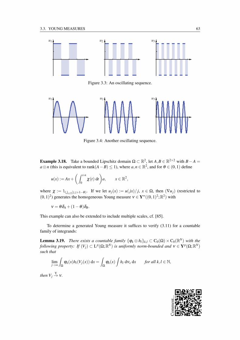
3.3. YOUNG MEASURES 63
Figure 3.3: An oscillating sequence.
Figure 3.4: Another oscillating sequence.
Example 3.18. Take a bounded Lipschitz domain Ω ⊂ R2, let A,B ∈ R2×2 with B−A =a⊗n (this is equivalent to rank(A−B)≤ 1), where a,n ∈ R2, and for θ ∈ (0,1) define
u(x) := Ax+(∫ x·n
0χ(t) dt
)a, x ∈ R2,
where χ := 1∪z∈Z[z,z+1−θ). If we let u j(x) := u( jx)/ j, x ∈ Ω, then (∇u j) (restricted to
(0,1)2) generates the homogeneous Young measure ν ∈ Y∞((0,1)2;R2) with
ν = θδA +(1−θ)δB.
This example can also be extended to include multiple scales, cf. [85].
To determine a generated Young measure it suffices to verify (3.11) for a countablefamily of integrands:
Lemma 3.19. There exists a countable family φk ⊗ hlk,l ⊂ C0(Ω)×C0(RN) with thefollowing property: If (Vj) ⊂ Lp(Ω;RN) is uniformly norm-bounded and ν ∈ Yp(Ω;RN)such that
limj→∞
∫Ω
φk(x)hl(Vj(x)) dx =∫
Ωφk(x)
∫hl dνx dx for all k, l ∈ N,
then VjY→ ν .
Com
men
t...
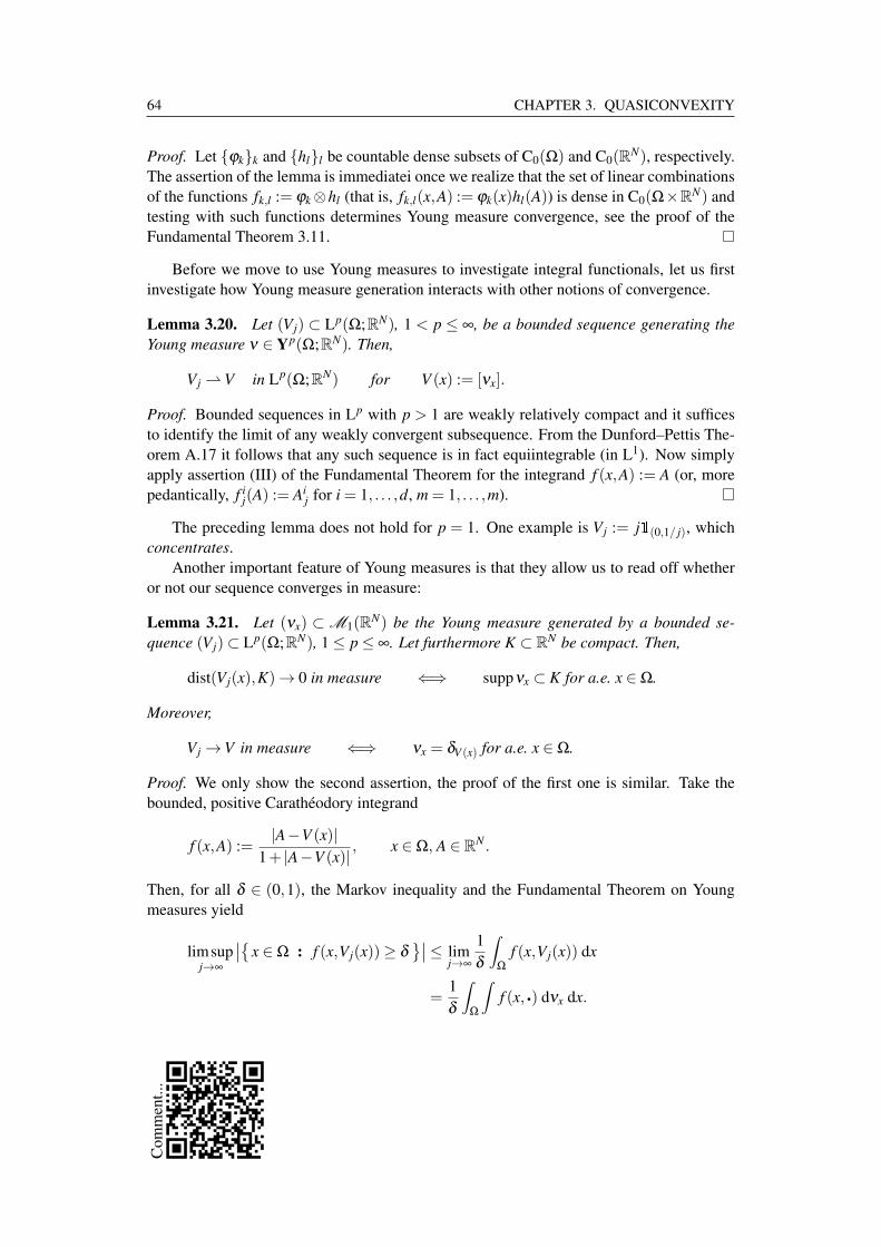
64 CHAPTER 3. QUASICONVEXITY
Proof. Let φkk and hll be countable dense subsets of C0(Ω) and C0(RN), respectively.The assertion of the lemma is immediatei once we realize that the set of linear combinationsof the functions fk,l := φk ⊗hl (that is, fk,l(x,A) := φk(x)hl(A)) is dense in C0(Ω×RN) andtesting with such functions determines Young measure convergence, see the proof of theFundamental Theorem 3.11.
Before we move to use Young measures to investigate integral functionals, let us firstinvestigate how Young measure generation interacts with other notions of convergence.
Lemma 3.20. Let (Vj) ⊂ Lp(Ω;RN), 1 < p ≤ ∞, be a bounded sequence generating theYoung measure ν ∈ Yp(Ω;RN). Then,
Vj V in Lp(Ω;RN) for V (x) := [νx].
Proof. Bounded sequences in Lp with p > 1 are weakly relatively compact and it sufficesto identify the limit of any weakly convergent subsequence. From the Dunford–Pettis The-orem A.17 it follows that any such sequence is in fact equiintegrable (in L1). Now simplyapply assertion (III) of the Fundamental Theorem for the integrand f (x,A) := A (or, morepedantically, f i
j(A) := Aij for i = 1, . . . ,d, m = 1, . . . ,m).
The preceding lemma does not hold for p = 1. One example is Vj := j1(0,1/ j), whichconcentrates.
Another important feature of Young measures is that they allow us to read off whetheror not our sequence converges in measure:
Lemma 3.21. Let (νx) ⊂ M1(RN) be the Young measure generated by a bounded se-quence (Vj)⊂ Lp(Ω;RN), 1 ≤ p ≤ ∞. Let furthermore K ⊂ RN be compact. Then,
dist(Vj(x),K)→ 0 in measure ⇐⇒ suppνx ⊂ K for a.e. x ∈ Ω.
Moreover,
Vj →V in measure ⇐⇒ νx = δV (x) for a.e. x ∈ Ω.
Proof. We only show the second assertion, the proof of the first one is similar. Take thebounded, positive Caratheodory integrand
f (x,A) :=|A−V (x)|
1+ |A−V (x)|, x ∈ Ω, A ∈ RN .
Then, for all δ ∈ (0,1), the Markov inequality and the Fundamental Theorem on Youngmeasures yield
limsupj→∞
∣∣x ∈ Ω : f (x,Vj(x))≥ δ∣∣≤ lim
j→∞
1δ
∫Ω
f (x,Vj(x)) dx
=1δ
∫Ω
∫f (x, q) dνx dx.
Com
men
t...

3.4. GRADIENT YOUNG MEASURES 65
On the other hand,∫Ω
∫f (x, q) dνx dx = lim
j→∞
∫Ω
f (x,Vj(x)) dx
≤ δ |Ω|+ limsupj→∞
∣∣x ∈ Ω : f (x,Vj(x))≥ δ∣∣.
The preceding estimates show that f (x,Vj(x)) converges to zero in measure if and onlyif ⟨ f (x, q),νx⟩ = 0 for L d-almost every x ∈ Ω, which is the case if and only if νx = δV (x)almost everywhere. We conclude by observing that f (x,Vj(x)) converges to zero in measureif and only if Vj converges to V in measure.
3.4 Gradient Young measures
The most important subclass of Young measures for our purposes is that of Young measuresthat can be generated by a sequence of gradients: Let ν ∈ Yp(Ω;Rm×d) (use RN = Rm×d
in the theory of the last section). We say that ν is a p-gradient Young measure, in sym-bols ν ∈ GYp(Ω;Rm×d), if there exists a bounded sequence (u j)⊂ W1,p(Ω;Rm) such that
∇u jY→ ν , i.e. the sequence (∇u j) generates ν . Note that it is not necessary that every se-
quence that generates ν is a sequence of gradients (which, in fact, is never the case). Wehave already considered examples of gradient Young measures in the previous section, seein particular Example 3.18.
Is it the case that every Young measure is a gradient Young measure? The answer isno, as can be easily seen: Let V ∈ (Lp ∩C∞)(Ω;Rm×d) with curlV (x) = 0 for some x ∈ Ω.Then, νx := δV (x) cannot be a gradient Young measure since for such measures it must hold
that [ν ] is a gradient itself: if there existed a sequence (u j) ⊂ W1,p(Ω;Rm) with ∇u jY→ ν ,
then ∇u j V by Lemma 3.20, and it would follow that curlV = 0. Consequently, for everyν ∈ GYp(Ω;Rm×d) there must exist u ∈ W1,p(Ω;Rm) with [ν ] = ∇u. In this case we callany such u an underlying deformation of ν .
We first show the following technical, but immensely useful, result about gradientYoung measures. Recall that we assume Ω to be open, bounded, and to have a Lipschitzboundary (to make the trace well-defined).
Lemma 3.22. Let ν ∈ GYp(Ω;Rm×d), 1 < p ≤ ∞, and let u ∈ W1,p(Ω;Rm) be an under-lying deformation of ν , i.e. [ν ] = ∇u. Then, there exists a sequence (u j) ⊂ W1,p(Ω;Rm)such that
u j|∂Ω = u|∂Ω and ∇u jY→ ν .
Furthermore, if 1 < p < ∞, in addition we can ensure that (∇u j) is p-equiintegrable.
Proof. Step 1. Since Ω is assumed to have a Lipschitz boundary, we can extend a generatingsequence (∇v j) for ν to all of Rd , so we assume (v j)⊂ W1,p(Rd ;Rm) with sup j ∥v j∥W1,p ≤C < ∞.
Com
men
t...

66 CHAPTER 3. QUASICONVEXITY
In the following, we need the maximal function M f : Rd → R∪ +∞ of f : Rd →R∪+∞, see Section A.5. With this tool at hand, consider the sequence
Vj := M(|v j|+ |∇v j|
), j ∈ N.
By Theorem A.29, (Vj) is uniformly bounded in Lp(Ω) and we may select a subsequence(not relabeled) such that Vj generates a Young measure µ ∈ Yp(Ω;Rm×d).
Next, define for h ∈ N the (nonlinear) truncation operator τh,
τhv :=
v if |v| ≤ h,h v|v| if |v|> h,
v ∈ R,
and let (φl)l ⊂ C∞(Ω) be a countable family that is dense in C(Ω).Step 2. Let 1< p<∞. Then, for fixed h∈N, the sequence (τhVj) j is uniformly bounded
in L∞(Ω) and so, by Young measure representation,
limh→∞
limj→∞
∫Ω
φl(x)|τhVj(x)|p dx = limh→∞
∫Ω
φl(x)∫
|τhv|p dµx(v) dx
=∫
Ωφl(x)
∫| q|p dµx dx,
where in the last step we used the monotone convergence lemma. Thus, for some diagonalsequence Wk := τkVj(k), we have that
limk→∞
∫Ω
φl(x) |Wk(x)|p dx =∫
Ωφl(x)
∫| q|p dµx dx for all l ∈ N.
Thus, |Wk|p converges weakly to x 7→ ⟨| q|p,µx⟩ in L1 and |Wk|pk is an equiintegrablefamily by the Dunford–Pettis Theorem. We can see also the equiintegrability in a moreelementary way as follows: For a Borel subset A ⊂ Ω take φ ∈ C∞(Ω) with 1A ≤ φ andestimate
limsupk→∞
∫A|Wk(x)|p dx ≤ lim
k→∞
∫Ω
φ(x) |Wk(x)|p dx =∫
Ωφ(x)
∫|v|p dµx(v) dx
by the L1-convergence of |Wk|p to x 7→ ⟨| q|p,µx⟩. The last integral tends to∫A
∫| q|p dµx dx
as φ ↓ 1A, which vanishes if |A| → 0. Thus the family Wkk is p-equiintegrable.Theorem A.29 implies that vk = v j(k) is Ck-Lipschitz on the set Gk := Wk ≤ k and by
the Kirszbraun Theorem A.27, we may extend vk to a function wk : Rd →Rm that is globallyLipschitz continuous with the same Lipschitz constant Ck and wk = vk in Gk. We have
|∇wk| ≤CWk in Ω
and thus |∇wk|k inherits the p-equiintegrable from Wkk.
Com
men
t...
3.5. HOMOGENEOUS GRADIENT YOUNG MEASURES 67
Moreover, by the Markov inequality,
|Ω\Gk| ≤∥Wk∥p
Lp
kp → 0 as k → ∞.
Therefore, for all φ ∈ C0(Ω) and h ∈ C0(Rm),∫Ω|φh(∇wk)−φh(∇vk)| dx ≤ ∥φ ⊗h∥∞ · |Ω\Gk| → 0.
Thus, since all such φ,h determine Young measure convergence (see the proof of the Fun-damental Theorem 3.11), we have shown that (∇wk) generates the same Young measure νas (∇v j) and additionally the family ∇wkk is p-equiintegrable.
Step 3. Since W1,p(Ω;Rm) embeds compactly into the space Lp(Ω;Rm) by the Rellich-Kondrachov Theorem A.23, we have wk → u in Lp. Let moreover (ρ j)⊂ C∞
c (Ω; [0,1]) be asequence of cut-off functions with the property that for the sets G j :=
x ∈ Ω : ρ j(x) = 1
it holds that |Ω\G j| → 0 as j → ∞. For
u j,k := ρ jwk +(1−ρ j)u ∈ W1,pu (Ω;Rm)
we observe ∇u j,k = ρ j∇wk +(1−ρ j)∇u+(wk −u)⊗∇ρ j.We only consider the case p < ∞ in the following; the proof for the case p = ∞ is in fact
easier. For every Caratheodory function f : Ω×Rm×d →R with | f (x,A)| ≤ M(1+ |A|p) wehave
limsupk→∞
∫Ω
∣∣ f (x,∇wk(x))− f (x,∇u j,k(x))∣∣ dx
≤ limsupk→∞
CM∫
Ω\G j
2+2|∇wk|p + |∇u|p + |wk −u|p · |∇ρ j|p dx
≤ limsupk→∞
CM∫
Ω\G j
2+2|∇wk|p + |∇u|p dx,
where C > 0 is a constant. However, by assumption, the last integrand is equiintegrable andhence
limj→∞
limsupk→∞
∫Ω
∣∣ f (x,∇wk(x))− f (x,∇u j,k(x))∣∣ dx = 0.
We can now select a diagonal sequence u j = u j,k( j) such that (∇u j) generates ν and satisfiesall requirements from the statement of the lemma. Note that the equiintegrability is notaffected by the cut-off procedure.
3.5 Homogeneous gradient Young measures
We next discuss some properties of homogeneous gradient Young measures, that is, ν ∈GYp(B(0,1);Rm×d) and νx is a.e. constant in x ∈ B(0,1). We simply write ν for any νx and[ν ] = [νx].
According to the following lemma the domain in the definition of homogeneous gradientYoung measures can be chosen as any bounded Lipschitz domain D ⊂ Rd (notice that forhomogeneous Young measures the averaged integral in (3.17) can be omitted).
Com
men
t...

68 CHAPTER 3. QUASICONVEXITY
Lemma 3.23 (Averaging). Let ν = (νx) ∈ GYp(Ω;Rm×d), where 1 ≤ p ≤ ∞, such that[ν ] = ∇u for some u ∈ W1,p(Ω;Rm) with affine boundary values. Then, for any boundedLipschitz domain D ⊂ Rd there exists a (unique) homogeneous gradient Young measureν ∈ GYp(D;Rm×d), i.e. ν = νy is constant in y ∈ D, such that∫
h dν = −∫
Ω
∫h dνx dx (3.17)
for all continuous h : Rm×d → R with p-growth (just continuity if p = ∞). This result re-mains valid if Ω = Qd = (−1/2,1/2)d , the d-dimensional unit cube and u has periodicboundary values.
Proof. We only explicitly treat the case that 1 ≤ p < ∞, the case p = ∞ is in fact easier.Let (u j) ⊂ W1,p(Ω;Rm) with u j(x)|∂Ω = Mx (in the sense of trace) for a fixed matrix
M ∈Rm×d such that ∇u jY→ ν , in particular sup j ∥∇u j∥Lp < ∞. Now choose for every j ∈N
a disjoint Vitali cover of D, see Theorem A.10,
D = Z ∪N( j)∪k=1
Ω(a( j)k ,r( j)
k ), |Z|= 0,
with a( j)k ∈ D, r( j)
k ≤ 1/ j (k = 1, . . . ,N( j)), and Ω(a,r) := a+ rΩ. Then define
v j(y) :=
r( j)k u j
(y−a( j)
k
r( j)k
)+Ma( j)
k if y ∈ Ω(a( j)k ,r( j)
k ),
0 otherwise,
y ∈ D.
We have v j ∈ W1,p(D;Rm) (it is easy to see that there are no jumps over the gluing bound-aries) and
∇v j(y) = ∇u j
(y−a( j)
k
r( j)k
)if y ∈ Ω(a( j)
k ,r( j)k ).
We can then use a change of variables to compute for all φ ∈ C0(D) and h ∈ C(Rm×d) withp-growth,∫
Dφ(y)h(∇v j(y)) dy =
N( j)
∑k=1
∫Ω(a( j)
k ,r( j)k )
φ(y)h(
∇u j
(y−a( j)
k
r( j)k
))dy
=N( j)
∑k=1
(r( j)k )dφ(a( j)
k )∫
Ωh(∇u j(x)) dx+O
(1j
)|D|
where we also used that φ is uniformly continuous. Letting j → ∞ and using that (Riemannsums)
limj→∞
N( j)
∑k=1
(r( j)k )dφ(a( j)
k ) =1|Ω|
∫D
φ(x) dx,
Com
men
t...
3.5. HOMOGENEOUS GRADIENT YOUNG MEASURES 69
we arrive at
limj→∞
∫D
φ(y)h(∇v j(y)) dy =∫
Dφ(x) dx · −
∫Ω
∫h(A) dνx dx. (3.18)
For φ = 1 and h(A) := |A|p, this gives
sup j ∥∇v j∥pLp = sup j ∥∇u j∥p
Lp < ∞.
Thus, there exists ν ∈ GYp(D;Rm) such that ∇v jY→ ν .
Using Lemma 3.22 we may moreover assume that (∇u j), and hence also (∇v j), is p-equiintegrable. Then, (3.18) implies∫
D
∫φ(y)h(A) dνy(A) dy =
∫D
φ(x) dx · −∫
Ω
∫h(A) dνx(A) dx
for all φ,h as above. This implies in particular that (νy) = ν is homogeneous. For φ = 1,we get (3.17).
The additional claim about Ω = Qd and an underlying deformation u with periodicboundary values follows analogously, since also in this case we can “glue” generating func-tions on a (special) covering.
Applying the preceding homogenization lemma to a gradient Young measure consistingonly of Dirac masses, we get the following result:
Lemma 3.24 (Riemann–Lebesgue lemma). Let u ∈ W1,p(Ω;Rm) have affine boundaryvalues, where 1 ≤ p ≤ ∞. Then, there exists a homogeneous gradient Young measureδ [∇u] ∈ GYp(Ω;Rm×d) (Ω ⊂ Rd any bounded Lipschitz domain) such that∫
h dδ [∇u] = −∫
Ωh(∇u(x)) dx (3.19)
for all continuous h : Rm×d → R with p-growth (just continuity if p = ∞). Furthermore,this result remains valid if Ω = Qd = (−1/2,1/2)d , the d-dimensional unit cube and u hasperiodic boundary values.
The following result is now easy to prove:
Lemma 3.25 (Jensen-type inequality). Let 1 < p ≤ ∞ and let ν ∈ GYp(Ω;Rm×d) be ahomogeneous gradient Young measure. Then, for all quasiconvex functions h : Rm×d → Rwith p-growth it holds that
h([ν ])≤∫
h dν . (3.20)
Notice that the conclusion of this lemma is trivial (and also holds for general Youngmeasures, not just the gradient ones) if h is convex. Thus (3.20) expresses the generalizedconvexity aspect of quasiconvexity.
Com
men
t...

70 CHAPTER 3. QUASICONVEXITY
Proof. Set A0 := [ν ] and let (u j) ⊂ W1,p(B(0,1);Rm) with ∇u jY→ ν , u j|∂B(0,1)(x) = A0x
for x ∈ ∂B(0,1) (in the sense of trace) and (∇u j) p-equiintegrable, the latter two conditionsbeing realizable by Lemma 3.22. Then, from the definition of quasiconvexity, we get
h(A0)≤ −∫
Ωh(∇u j) dx.
Passing to the Young measure limit as j → ∞ on the right-hand side, for which we note thath(∇u j) is equiintegrable by the growth assumption on h, we arrive at
h(A0)≤ −∫
Ω
∫h dν dx =
∫h dν ,
which already is the sought inequality.
The last result will be of crucial importance in proving weak lower semicontinuity inthe next section. It is remarkable that the converse also holds, i.e. the validity of (3.20)for all quasiconvex h with p-growth (no condition if p = ∞) precisely characterizes theclass of (homogeneous) gradient Young measures in the class of all (homogeneous) Youngmeasures; this is the content of the Kinderlehrer–Pedregal Theorem 5.12, which we willmeet in Chapter 5.
Corollary 3.26. Let 1 < p ≤ ∞ and let ν ∈ GYp(Ω;Rm×d) be a homogeneous gradientYoung measure. Then, for all quasiaffine functions h : Rm×d → R with p-growth it holdsthat
h([ν ]) =∫
h dν .
Proof. Apply the preceding lemma to h and −h.
In particular, the preceding corollary applies to the determinant and, more generally,minors, see Corollary 3.9.
3.6 Lower semicontinuity
After our detour through Young measure theory, we now return to the central subject of thischapter, namely to minimization problems of the formF [u] :=
∫Ω
f (x,∇u(x)) dx → min,
over all u ∈ W1,p(Ω;Rm) with u|∂Ω = g,
where Ω ⊂ Rd is a bounded Lipschitz domain, 1 < p < ∞, the integrand f : Ω×Rm ×Rm×d → R has p-growth,
| f (x,A)| ≤ M(1+ |A|p) for some M > 0,
Com
men
t...

3.6. LOWER SEMICONTINUITY 71
and g ∈ W1−1/p,p(∂Ω;Rm) specifies the boundary values. In Chapter 2 we solved this prob-lem via the Direct Method of the calculus of variations, a coercivity result, and, crucially,the Lower Semicontinuity Theorem 2.7. In this section, we recycle the Direct Method andthe coercivity result, but extend lower semicontinuity to quasiconvex integrands; some mo-tivation for this was given at the beginning of the chapter.
Let us first consider how we could approach the proof of lower semicontinuity (it shouldbe clear that the proof via Mazur’s Lemma that we used for the convex lower semicontinuitytheorem, does not extend). Assume we have a sequence (u j) ⊂ W1,p(Ω;Rm) such thatu j u in W1,p and we want to show lower semicontinuity of our functional F . If weassume that our (norm-bounded) sequence ∇u j also generates the gradient Young measureν ∈ GYp(Ω;Rm×d), which is true up to a subsequence, and that the sequence of integrands( f (x,∇u j(x))) j is equiintegrable, then we already have a limit:
F [u j]→∫
Ω
∫f (x,A) dνx(A) dx.
This is useful, because it now suffices to show the inequality∫f (x, q) dνx ≥ f (x,∇u(x)) dx
for almost every x ∈ Ω, to conclude lower semicontinuity. Now, this inequality is close tothe Jensen-type inequality (3.20) for gradient Young measures from Lemma 3.25, and wealready explained how this is related to (quasi)convexity. The only difference in comparisonto (3.20) is that here we need to “localize” in x ∈ Ω and make νx a gradient Young measurein its own right. This is accomplished via the fundamental blow-up technique (also called“localization”):
Lemma 3.27 (Blow-up technique). Let 1 ≤ p < ∞ and let ν = (νx) ∈ GYp(Ω;Rm×d) bea gradient Young measure. Then, for almost every x0 ∈ Ω, νx0 ∈ GYp(B(0,1);Rm×d) is ahomogeneous gradient Young measure in its own right.
Proof. Take a countable collection φk⊗hlk,l as in Lemma 3.19. Let x0 ∈Ω be a Lebesguepoint of all the functions x 7→ ⟨hl,νx⟩ (l ∈ N), that is,
limr↓0
∫B(0,1)
∣∣⟨hl,νx0+ry⟩−⟨hl,νx0
⟩∣∣ dy = 0.
By Theorem A.9, almost every x ∈ Ω has this property. Then, at such a Lebesgue point x0,set
v(r)j (y) :=u j(x0 + ry)− [u j]B(x0,r)
r, y ∈ B(0,1),
where [u]B(x0,r) := −∫
B(x0,r) u dx.For φk, hl we get∫
B(0,1)φk(y)hl(∇v(r)j (y)) dy =
∫B(0,1)
φk(y)hl(∇u j(x0 + ry)) dy
=1rd
∫B(x0,r)
φk
(x− x0
r
)hl(∇u j(x)) dx
Com
men
t...
72 CHAPTER 3. QUASICONVEXITY
after a change of variables. Letting j → ∞ and then r ↓ 0, we get
limr↓0
limj→∞
∫B(0,1)
φk(y)hl(∇v(r)j (y)) dy = limr↓0
1rd
∫B(x0,r)
φk
(x− x0
r
)⟨hl,νx
⟩dx
= limr↓0
∫B(0,1)
φk(y)⟨hl,νx0+ry
⟩dx
=∫
B(0,1)φk(y)
⟨hl,νx0
⟩dy,
the last convergence following from the Lebesgue point property of x0. Moreover,∫B(0,1)
|∇v(r)j |p dy =∫
B(0,1)|∇u j(x0 + ry)|p dy =
1rd
∫B(x0,r)
|∇u j(x)|p dx
and the last integral is uniformly bounded in j (for fixed r). Denote by λ ∈ M (Ω;Rm) theweak* limit of the measures |∇u j|pL d Ω, which exists after taking a subsequence. If werequire of x0 additionally that
limsupr↓0
λ (B(x0,r))rd < ∞,
which hold at L d-almost every x0 ∈ Ω, then
limsupr↓0
limj→∞
∫B(0,1)
|∇v(r)j |p dy < ∞.
Since also [v(r)j ]B(0,1) = 0, the Poincare inequality from Theorem A.21 yields that there exists
a diagonal sequence w j := vR( j)J( j) that is uniformly bounded in W1,p(B(0,1);Rm) and such
that for all k, l ∈ N,
limj→∞
∫B(0,1)
φk(y)hl(∇w j(y)) dy =∫
B(0,1)φk(y)
⟨hl,νx0
⟩dy.
Therefore, ∇w jY→ νx0 by Lemma 3.19, where we now understand νx0 as a homogeneous
(gradient) Young measure on B(0,1).
Our main weak lower semicontinuity is then a straightforward application of the theorydeveloped so far. The first result of this type is due to Morrey from 1952 (for integralfunctionals defined on W1,∞ and under additional technical assumptions), but our Youngmeasure approach allows us to prove a fairly general result, which was first established byAcerbi–Fusco (using different methods, however).
Theorem 3.28 (Acerbi–Fusco 1984). Let 1 < p < ∞ and let f : Ω×Rm×d → [0,∞) bea Caratheodory integrand with p-growth and such that f (x, q) is quasiconvex for everyfixed x ∈ Ω. Then, the corresponding functional F is weakly lower semicontinuous onW1,p(Ω;Rm).
Com
men
t...
3.6. LOWER SEMICONTINUITY 73
We first need the following result about Young measures:
Proposition 3.29. Let (Vj) ⊂ Lp(Ω;RN), 1 ≤ p ≤ ∞, be a bounded sequence generatingthe Young measure ν ∈ Yp(Ω;RN), and let f : Ω×RN → [0,∞) be any Caratheodory inte-grand (not necessarily satisfying the equiintegrability property in (iii) of the FundamentalTheorem). Then, it holds that
liminfj→∞
∫Ω
f (x,Vj(x)) dx ≥⟨⟨
f ,ν⟩⟩.
Proof of Theorem 3.28. For M ∈N define fM(x,A) :=min( f (x,A),M). Then, (III) from theFundamental Theorem is applicable with fM and we get∫
ΩfM(x,Vj(x)) dx →
⟨⟨fM,ν
⟩⟩=∫
Ω
∫fM(x,A) dνx(A) dx.
Since f ≥ fM , we have
liminfj→∞
∫Ω
f (x,Vj(x)) dx ≥⟨⟨
fM,ν⟩⟩.
We conclude by letting M ↑ ∞ and using the monotone convergence lemma.
Proof. Let (∇u j) ⊂ W1,p(Ω;Rm) with u j u in W1,p. Assume that (∇u j) generates thegradient Young measure ν = (νx) ∈ GYp(Ω;Rm×d), for which it holds that [ν ] = ∇u. Thisis only true up to a (non-relabeled) subsequence, but if we can establish the lower semi-continuity for every such subsequence it follows that the result also holds for the originalsequence.
From Proposition 3.29 we get
liminfj→∞
∫Ω
f (x,∇u j(x)) dx ≥⟨⟨
f ,ν⟩⟩=∫
Ω
∫f (x,A) dνx(A) dx.
Now, for almost every x ∈ Ω, we can consider νx as a homogeneous Young measure inGYp(B(0,1);Rm×d) by the Blow-up Lemma 3.27. Thus, the Jensen-type inequality fromLemma 3.25 reads∫
f (x,A) dνx(A)≥ f (x,∇u(x)) for a.e. x ∈ Ω.
Combining, we arrive at
liminfj→∞
F [u j]≥ F [u],
which is what we wanted to show.
At this point is is worthwhile to reflect on the role of Young measures in the proof ofthe preceding result, namely that they allowed us to split the argument into two parts: First,we passed to the limit in the functional via the Young measure. Second, we establisheda Jensen-type inequality, which then yielded the lower semicontinuity inequality. It is re-markable that the Young measure preserves exactly the “right” amount of information toserve as an intermediate object.
We can now sum up and prove existence to our minimization problem:
Com
men
t...

74 CHAPTER 3. QUASICONVEXITY
Theorem 3.30. Let f : Ω×Rm×d → [0,∞) be a Caratheodory integrand such that f hasp-growth, satisfies the p-coercivity estimate
µ|A|p −µ−1 ≤ f (x,A) for some µ > 0,
and is quasiconvex in its second argument. Then, the associated functional F has a mini-mizer over the space W1,p
g (Ω;Rm), where g ∈ W1−1/p,p(∂Ω;Rm).
Proof. This follows directly by combining the Direct Method from Theorem 2.3 with thecoercivity result in Proposition 2.6 and the Lower Semicontinuity Theorem 3.28.
The following result shows that quasiconvexity is also necessary for weak lower semi-continuity; we only state and show this for x-independent integrands, but we note that it alsoholds for x-dependent ones by a localization technique.
Proposition 3.31. Let f : Rm×d → R have p-growth. If the associated functional
F [u] :=∫
Ωf (∇u(x)) dx, u ∈ W1,p(Ω;Rm),
is weakly lower semicontinuous (with or without fixed boundary values), then f is quasi-convex.
Proof. We may assume that B(0,1)⋐Ω, otherwise we can translate and rescale the domain.Let A ∈ Rm×d and ψ ∈ W1,∞
0 (B(0,1);Rm). We need to show
h(A)≤ −∫
B(0,1)h(A+∇ψ(z)) dz.
Take for every j ∈ N a Vitali cover of B(0,1), see Theorem A.10,
B(0,1) = Z ∪N( j)∪k=1
B(a( j)k ,r( j)
k ), |Z|= 0,
with a( j)k ∈ B(0,1), r( j)
k ≤ 1/ j (k = 1, . . . ,N( j)), and fix a smooth function h : Ω\B(0,1)→Rm with h(x) = Ax for x ∈ ∂B(0,1) (and h|∂Ω equal to the prescribed boundary values ifthere are any). Define
u j(x) := Ax+ r( j)k ψ
(x−a( j)
k
r( j)k
)if x ∈ B(a( j)
k ,r( j)k ),
and u j := h on Ω\B(0,1). Then, it is not hard to see that u j u in W1,p for
u(x) =
Ax if x ∈ B(0,1),h(x) if x ∈ Ω\B(0,1),
x ∈ Ω.
Com
men
t...
3.7. INTEGRANDS WITH u-DEPENDENCE 75
Thus, the lower semicontinuity yields, after eliminating the constant part of the functionalon Ω\B(0,1),∫
B(0,1)f (A) dx ≤ liminf
j→∞
∫B(0,1)
f (∇u j(x)) dx
= liminfj→∞ ∑
k
∫B(a( j)
k ,r( j)k )
f(
A+∇ψ(
x−a( j)k
r( j)k
))dx
= liminfj→∞ ∑
kr( j)
k
∫B(0,1)
f (A+∇ψ(y)) dy
=∫
B(0,1)f (A+∇ψ(y)) dy
since ∑k r( j)k = 1. This is nothing else than quasiconvexity.
We note that also for quasiconvex integrands, our results about the Euler–Lagrangeequations hold just the same (if we assume the same growth conditions).
3.7 Integrands with u-dependence
One very useful feature of our Young measure approach is that it allows to derive a lowersemicontinuity result for u-dependent integrands with minimal additional effort. So con-sider F [u] :=
∫Ω
f (x,u(x),∇u(x)) dx → min,
over all u ∈ W1,p(Ω;Rm) with u|∂Ω = g,
where Ω ⊂ Rd is a bounded Lipschitz domain, 1 < p < ∞, and the Caratheodory integrandf : Ω×Rm ×Rm×d → R satisfies the p-growth bound
| f (x,v,A)| ≤ M(1+ |v|p + |A|p) for some M > 0, (3.21)
and g ∈ W1−1/p,p(∂Ω;Rm).The main idea of our approach is to consider Young measures generated by the pairs
(u j,∇u j) ∈ Rm+md . We have the following result:
Lemma 3.32. Let (u j) ⊂ Lp(Ω;RM) and (Vj) ⊂ Lp(Ω;RN) be norm-bounded sequencessuch that
u j → u pointwise a.e. and VjY→ ν = (νx) ∈ Yp(Ω;RN).
Then, (u j,Vj)Y→ µ = (µx) ∈ Yp(Ω;RM+N) with
µx = δu(x)⊗νx for a.e. x ∈ Ω,
Com
men
t...

76 CHAPTER 3. QUASICONVEXITY
that is,∫Ω
f (x,u j(x),Vj(x)) dx →∫
Ω
∫f (x,u(x),A) dνx(A) dx (3.22)
for all Caratheodory f : Ω×RM ×RN → R satisfying the p-growth bound (3.21).
Proof. By a similar density argument as in the proof of Lemma 3.27, it suffices to showthe convergence (3.22) for f (x,v,A) = φ(x)ψ(v)h(A), where φ ∈ C0(Ω), ψ ∈ C0(RM),h ∈ C0(RN). We already know by assumption
h(Vj)∗(x 7→
⟨h,νx
⟩)in L∞.
Furthermore, ψ(u j)→ ψ(u) almost everywhere and thus strongly in L1 since ψ is bounded.Thus, since the product of a L∞-weakly* converging sequence and a L1-strongly convergingsequence converges itself weakly* in the sense of measures,∫
Ωφ(x)ψ(u j(x))h(Vj(x)) dx →
∫Ω
φ(x)ψ(u(x))⟨h,νx
⟩dx,
which is (3.22) for our special f . This already finishes the proof.
The trick of the preceding lemma is that in our situation, where Vj = ∇u jY→ ν ∈
GYp(Ω;Rm×d), it allows us to “freeze” u(x) in the integrand. Then, we can apply theJensen-type inequality from Lemma 3.25 just as we did in Theorem 3.28 to get:
Theorem 3.33. Let f : Ω×Rm ×Rm×d → R be a Caratheodory integrand with p-growth(in v and A), i.e. | f (x,v,A)| ≤ M(1+ |v|p + |A|p) for some M > 0, 1 < p < ∞. Assumefurthermore that f (x,v, q) is quasiconvex for every fixed (x,v) ∈ Ω×Rm. Then, the corre-sponding functional F is weakly lower semicontinuous on W1,p(Ω;Rm).
Remark 3.34. It is not too hard to extend the previous theorem to integrands f satisfyingthe more general growth condition
| f (x,v,A)| ≤ M(1+ |v|q + |A|p)
for a 1 ≤ q < p/(d− p). By the Sobolev Embedding Theorem A.22, u j → u in Lq (strongly)for all such q and thus Lemma 3.32 and then Theorem 3.33 can be suitably generalized.
3.8 Regularity of minimizers
At the end of Section 2.5 we discussed the failure of regularity for vector-valued problems.In particular, we mentioned various counterexamples to regularity. Upon closer inspection,however, it turns out that in all counterexamples, the points where regularity fails form aclosed set. This is not a coincidence.
Another issue was that all regularity theorems discussed so far require (strong) con-vexity of the integrand and our discussion so far has shown that convexity is not a good
Com
men
t...

3.8. REGULARITY OF MINIMIZERS 77
notion for vector-valued problems (however, much of the early regularity theory for vector-valued problems focused on convex problems, we will not elaborate on this aspect here). Toremedy this, we need a new notion, which will take over from strong convexity in regular-ity theory: A locally bounded Borel-measurable function h : Rm×d → R is called strongly(2-)quasiconvex if there exists µ > 0 such that
A 7→ h(A)−µ|A|2 is quasiconvex.
Equivalently, we may require that
µ∫
B(0,1)|∇ψ(z)|2 dz ≤
∫B(0,1)
h(A+∇ψ(z))−h(A) dz
for all A ∈ Rm×d and all ψ ∈ W1,∞0 (B(0,1);Rm).
The most well-known regularity result in this situation is by Evans from 1986 (there issignificant overlap with work by Acerbi & Fusco in the same year):
Theorem 3.35 (Evans 1986). Let f : Rm×d →R be of class C2, strongly quasiconvex, andassume that there exists M > 0 such that
D2A f (A)[B,B]≤ M|B|2 for all A,B ∈ Rm×d .
Let u ∈ W1,2g (Ω;Rm) be a minimizer of F over W1,2
g (Ω;Rm) where g ∈ W1/2,2(∂Ω;Rm).Then, there exists a relatively closed singular set Σu ⊂ Ω with |Σu| = 0 and it holds thatu ∈ C1,α
loc (Ω\Σu) for all α ∈ (0,1).
The proof is long and builds on earlier work of Almgren and De Giorgi in GeometricMeasure Theory.
The result is called a “partial regularity” result because the regularity does not holdeverywhere. It should be noted that while the scalar regularity theory was essentially atheory for PDEs, and hence applies to all solutions of the Euler–Lagrange equations, thisis not the case for the present result: There is no regularity theory for critical points of theEuler–Lagrange equation for a quasiconvex or even polyconvex (see next chapter) integralfunctional. This was shown by Muller & Sverak in 2003 [87] (for the quasiconvex case) andSzekelyhidi Jr. in 2004 [107] (for the polyconvex case). We finally remark that sometimesbetter estimates on the “smallness” of Σu than merely |Σu| = 0 are available. In fact, forstrongly convex integrands it can be shown that the (Hausdorff-)dimension of the singularset is at most d − 2, this is actually within reach of our discussion in Section 2.5, becausewe showed W2,2
loc-regularity, and general properties of such functions imply the conclusion,see Chapter 2 of [49]. In the strongly quasiconvex case, much less is known, but at least forminimizers that happen to be W1,∞ it was established in 2007 by Kristensen & Mingionethat the dimension of the singular set is strictly less than d, see [66]. Many other questionsare open.
Com
men
t...

78 CHAPTER 3. QUASICONVEXITY
Notes and historical remarks
The notion of quasiconvexity was first introduced in Morrey’s fundamental paper [79] andlater refined by Meyers in [76]. The results about null-Lagrangians, in particular Lemma 3.8and Lemma 3.10, go back to Morrey [80], Reshetnyak [95] and Ball [4]. Our proof is basedon the idea that certain combinations of derivatives might have good convergence propertieseven if the individual derivatives do not. This is also pivotal for so-called compensatedcompactness, which originated in work of Tartar [109,110] and Murat [88,89], in particularin their celebrated Div–Curl Lemma, this is detailed in [41]. It is quite remarkable that onecan prove Brouwer’s fixed point theorem using the fact that minors are null-Lagrangians,see Theorem 8.1.3 in [42]. Proposition 3.6 is originally due to Morrey [80], we follow thepresentation in [11]. We also remark that if only r = p, then a weaker version of Lemma 3.10is true where we only have convergence of the minors in the sense of distributions, seeTheorem 8.20 in [29].
The convexity properties of the quadratic function A 7→ MA : A, where M is a fourth-order tensor (or, equivalently, a matrix in Rmd×md) has received considerable attention be-cause it corresponds to a linear Euler–Lagrange equation. In this case, quasiconvexity andrank-one convexity are the same. Moreover, even polyconvexity (see next chapter) is equiv-alent to quasiconvexity (and rank-one convexity) if d = 2 or m = 2, but this does not holdanymore for d,m≥ 3. These results together with pointers to the vast literature can be foundin Section 5.3.2 in [29].
A more general result on why convexity is inadmissible for realistic problems in non-linear elasticity can be found in Section 4.8 of [22].
The result that rank-one convex functions are locally Lipschitz continuous is well-known for convex functions, see for example Corollary 2.4 in [39] and an adapted versionfor rank-one convex (even separately convex) functions is in Theorem 2.31 in [29]. Ourproof with a quantitative bound is from Lemma 2.2 in [11].
The Fundamental Theorem of Young Measure Theory 3.11 has seen considerable evolu-tion since its original proof by Young in the 1930s and 1940s [115–117]. It was popularizedin the calculus of variations by Tartar [110] and Ball [6]. Further, much more general,versions have been contributed by Balder [3], also see [21] for probabilistic applications.
The Ball–James rigidity theorem 5.11 is from [9].Lemma 3.22 is an expression of the well-known decomposition lemma from [44], an-
other version is in [63]. The blow-up technique is related to the use of tangent measures inGeometric Measure Theory, see for example [72].
Many results in this chapter are formulated for Caratheodory integrands continue tohold for f : Ω×RN →R that are Borel measurable and lower semicontinuous in the secondargument, so called normal integrands, see [16] and [43].
It is possible to prove the Lower Semicontinuity Theorem 3.28 for quasiconvex inte-grands without the use of Young measures, see for instance Chapter 8 in [29] for such anapproach. However, many of the ideas are essentially the same, they are just carried out di-rectly without the intermediate steps of Young measures. However, Young measures allowone to very clearly organize and compartmentalize these ideas, which aids the understand-
Com
men
t...
3.8. REGULARITY OF MINIMIZERS 79
ing of the material. We will also use Young measures later for the relaxation of non-lowersemicontinuous functionals. More on lower semicontinuity and Young measures can befound in the book [94]. The first use of Young measures to investigate questions of lowersemicontinuity for quasiconvex integral functionals seems to be [58].
Kruzık [67] showed the curious property that for a quasiconvex h : Rm×d →R with m ≥3, d ≥ 2 the function A 7→ h(AT ) may not be quasiconvex. The proof is based on Sverak’sexample of a rank-one convex function that is not quasiconvex (for the same dimensions),which we will present in Example 5.15 in Chapter 5.
If the integrand has critical negative growth, then lower semicontinuity only holds ifthe boundary values are fixed along a sequence or if one imposes quasiconvexity at theboundary, see [14] for a recent survey article discussing this topic.
Laurence Chisholm Young originally introduced the objects that are now called Youngmeasures as “generalized curves/surfaces” in the late 1930s and early 1940s [115–117]to treat problems in the calculus of variations and optimal control theory that could not besolved using classical methods. His book [118] explains these objects and their applicationsin great detai (in particular, our “sailing against the wind” example from Section 1.7 is fromthere).
In Chapter 5 we will consider relaxation problems formulated using Young measures.Further, Young measures have provided a convenient framework to describe fine phase mix-tures in the theory of microstructure. A second avenue of development—somewhat differentfrom Young’s original intention—is to use Young measures as a technical tool only (that iswithout them appearing in the final statement of a result). This approach is in fact quite oldand was probably first adopted in a series of articles by McShane from the 1940s [73–75].There, the author first finds a generalized Young measure solution to a variational problem,then proves additional properties of the obtained Young measures, and finally concludesthat these properties entail that the generalized solution is in fact classical. This idea ex-hibits some parallels to the hugely successful approach of first proving existence of a weaksolution to a PDE and then showing that this weak solution has (in some cases) additionalregularity.
Several people contributed to Young measure theory from the 1970s onward, includ-ing Berliocchi & Lasry [16], Balder [3], Ball [6] and Kristensen [64], among many others.An important breakthrough in this respect was the characterization of the class of Youngmeasures generated by sequences of gradients in the early 1990s by Kinderlehrer and Pe-dregal [57, 59], see Theorem 5.12. Their result places gradient Young measures in dualitywith quasiconvex functions via Jensen-type inequalities (another work in this direction isSychev’s article [106]). Young measures can also be used to show regularity, see the recentwork by Dolzmann & Kristensen [37]. Carstensen & Roubıcek [20] considered numericalapproximations.
Another branch of Young measure theory started in the late 1970s and early 1980s, whenTartar [109,110,112] and Murat [88–90] developed the theory of compensated compactnessand were able to settle many open problems in the theory of hyperbolic conservation laws;another important contributor here was DiPerna, see for example [35]. A key point of thisstrategy is to use the good compactness properties of Young measures to pass to limits easily
Com
men
t...
80 CHAPTER 3. QUASICONVEXITY
in nonlinear quantities and then to deduce from pointwise and differential constraints on thegenerating sequences that the Young measure collapses to a point mass, corresponding toa classical function (so no oscillation phenomena occurred). Moreover, in this situationweak convergence improves to convergence in measure (or even in norm), hence the namecompensated compactness. Extensions of Young measures that allow to pass to the limit inquadratic expressions have been developed by Tartar [111] under the name “H-measures”and, independently, by Gerard [47], who called them “micro-local defect measures”, cf. thesurvey articles [45, 113].
The theory of Young measures is now very mature and there are several monographs [21,94, 96] that give overviews over the theory from different points of view.
Com
men
t...

Chapter 4
Polyconvexity
At the beginning of Chapter 3 we saw that convexity cannot hold concurrently with frame-indifference (and a mild positivity condition). Thus, we were lead to consider quasiconvexintegrands. However, while quasiconvexity is of huge importance in the theory of the cal-culus of variations, our Lower Semicontinuity Theorem 3.28 has one major drawback: weneeded to require the p-growth bound
| f (x,A)| ≤ M(1+ |A|p), x ∈ Ω, A ∈ Rd×d ,
for some M > 0 and 1< p<∞. Unfortunately, this is not a realistic assumption for nonlinearelasticity because it ignores the fact that infinite compressions should cost infinite energy.Indeed, realistic integrands have the property that
f (A)→+∞ as det A ↓ 0
and
f (A) = +∞ if det A ≤ 0.
For example, the family of matrices
Aα :=(
1 00 α
), α > 0,
satisfies det Aα ↓ 0 as α ↓ 0, but |Aα | remains uniformly bounded, so the above p-growthbound cannot hold.
The question whether the Lower Semicontinuity Theorem 3.28 for quasiconvex inte-grands can be extended to integrands with the above growth is currently a major unsolvedproblem, see [7]. For the time being, we have to confine ourself to a more restrictive notionof convexity if we want to allow for the above “elastic” growth. This type of convexity iscalled polyconvexity by John Ball in [4], who proved the corresponding existence theoremfor minimization problems and enabled a mature mathematical treatment of nonlinear elas-ticity theory, including the realistic Mooney–Rivlin and Ogden materials, see Section 1.4and Examples 4.3, 4.4.
Com
men
t...

82 CHAPTER 4. POLYCONVEXITY
We will only look at the three-dimensional theory because it is by far the most physi-cally important case and because this restriction eases the notational burden; however, otherdimensions can be treated as well, we refer to the comprehensive treatment in [29].
4.1 Polyconvexity
A continuous integrand h : R3×3 →R∪+∞ (now we allow the value +∞) is called poly-convex if it can be written in the form
h(A) = H(A,cofA,det A), A ∈ R3×3,
where H : R3×3×R3×3×R→R∪+∞ is convex. Here, cofA denotes the cofactor matrixas defined in Appendix A.1.
While convexity obviously implies polyconvexity, the converse is clearly false. How-ever, we have:
Proposition 4.1. A polyconvex h : R3×3 → R (not taking the value +∞) is quasiconvex.
Proof. Let h be as stated and let ψ ∈ W1,∞(B(0,1);R3) with ψ(x)|∂B(0,1) = Ax. Then, usingJensen’s inequality
−∫
B(0,1)h(∇ψ) dx = −
∫B(0,1)
H(∇ψ,cof∇ψ,det∇ψ) dx
≥ H(−∫
B(0,1)∇ψ dx,−
∫B(0,1)
cof∇ψ dx,−∫
B(0,1)det∇ψ dx
)= H(A,cofA,det A) = h(A),
where for the last line we used the fact that minors are null-Lagrangians as proved inLemma 3.8.
At this point we have seen all four major convexity conditions that play a role in themodern calculus of variations. They can be put into a linear order by implications:
convexity ⇒ polyconvexity ⇒ quasiconvexity ⇒ rank-one convexity
While in the scalar case (d = 1 or m = 1) all these notions are equivalent, in higher dimen-sions the reverse implications do not hold in general. Clearly, the determinant function ispolyconvex but not convex. However, the fact that the notions of polyconvexity, quasicon-vexity, and rank-one convexity are all different in higher dimensions, are non-trivial. Thefact that rank-one convexity does not imply quasiconvexity, at least for d ≥ 2, m ≥ 3, is thesubject of Sverak’s famous counterexample, see Example 5.15. The case d = m = 2 is stillopen and one of the major unsolved problems in the field. Here we discuss an example of aquasiconvex, but not polyconvex function:
Com
men
t...

4.2. EXISTENCE OF MINIMIZERS 83
Example 4.2 (Alibert–Dacorogna–Marcellini). Recall from Example 3.5 the Alibert–Dacorogna–Marcellini function
hγ(A) := |A|2(|A|2 −2γ det A
), A ∈ R2×2.
It can be shown that hγ is polyconvex if and only if |γ| ≤ 1. Since it is quasiconvex if andonly if |γ| ≤ γQC, where γQC > 1, we see that there are quasiconvex functions that are notpolyconvex. See again Section 5.3.8 in [29] for details.
Example 4.3 (Mooney–Rivlin materials). Functions W of the form
W (F) := a|F |2 +b|cofF |2 +Γ(detF),
with a,b > 0 and Γ(d) = αd2 −β logd for α,β > 0 are polyconvex. This is obvious oncewe realize that Γ is convex. Such energy functionals model Mooney–Rivlin materials or, ifb = 0 neo-Hookean materials.
Example 4.4 (Ogden materials). Functions W of the form
W (F) :=M
∑i=1
ai tr[(FT F)γi/2]+ N
∑j=1
b j tr cof[(FT F)δ j/2]+Γ(detF), F ∈ R3×3,
where ai > 0, γi ≥ 1, b j > 0, δ j ≥ 1, and Γ : R → R∪ +∞ is a convex function withΓ(d) → +∞ as d ↓ 0, Γ(d) = +∞ for s ≤ 0 and good enough growth from below, can beshown to be polyconvex. These stored energy functionals correspond to so-called Ogdenmaterials and occur in a wide range of elasticity applications, see [22] for details.
It can also be shown that in three dimensions convex functions of certain combinationsof the singular values of a matrix (the singular values of A are the square roots of the eigen-values of AT A) are polyconvex, see Section 5.3.3 in [29] for details.
4.2 Existence of minimizers
Let Ω ⊂ R3 be a connected bounded Lipschitz domain. In this section we will prove exis-tence of a minimizer of the variational problemF [u] :=
∫Ω
W (x,∇u(x))−b(x) ·u(x) dx → min,
over all u ∈ W1,p(Ω;R3) with det∇u > 0 a.e. and u|∂Ω = g,(4.1)
where W : Ω×R3×3 → R∪+∞ is Caratheodory and W (x, q) is polyconvex for almostevery x ∈ Ω. Thus,
W (x,A) =W(x,A,cofA,det A), (x,A) ∈ Ω×R3×3,
Com
men
t...
84 CHAPTER 4. POLYCONVEXITY
for W : Ω×R3×3 ×R3×3 ×R→ R∪+∞ with W(x, q, q, q) jointly convex and continuousfor almost every x ∈ Ω. As the only upper growth assumptions on W we impose
W (x,A)→+∞ as det A ↓ 0,
W (x,A) = +∞ if det A ≤ 0.
Furthermore, we assume as usual that g ∈ W1−1/p,p(∂Ω;R3) and that b ∈ Lq(Ω;R3) where1/p+ 1/q = 1. The exponent p > 1 will remain unspecified for now. Later, when weimpose conditions on the coercivity of W , we will also specify p.
The first lower semicontinuity result is relatively straightforward:
Theorem 4.5. If in addition to the above assumptions it holds that
µ|A|p −µ−1 ≤W (x,A) for some µ > 0 and p > 3, (4.2)
then the minimization problem (4.1) has at least one solution in the space
A :=
u ∈ W1,p(Ω;R3) : det∇u > 0 a.e. and u|∂Ω = g,
whenever this set is non-empty.
Proof. We apply the usual Direct Method. For a minimizing sequence (u j) ⊂ A withF [u j]→ min, we get from the coercivity estimate (4.2) in conjunction with the Poincare–Friedrichs inequality (and the fixed boundary values) that for any δ > 0,∫
ΩW (x,∇u j)−b(x) ·u j(x) dx
≥ µ∥∇u j∥pLp −µ−1|Ω|−∥b∥Lq · ∥u j∥Lp
≥ µC∥u j∥p
W1,p −µC∥g∥p
W1−1/p,p −|Ω|µ
− 1δq
∥b∥qLq −
δp∥u j∥p
W1,p .
Choosing δ = pµ/(2C), we arrive at
supj∈N
∥u j∥W1,p ≤C(
supj∈N
F [u j]+1).
Thus, we may select a subsequence (not relabeled) such that u j u in W1,p(Ω;R3).Now, by Lemma 3.10 and p > 3,
det∇u j det∇u in Lp/3 and
cof∇u j cof∇u in Lp/2.
Thus, an argument entirely analogous to the proof of Theorem 2.7 (note that in that theoremwe did not need any upper growth condition) yields that the hyperelastic part of F ,
u 7→∫
ΩW (x,∇u j) dx =
∫ΩW(x,∇u j,cof∇u j,det∇u j) dx
Com
men
t...
4.2. EXISTENCE OF MINIMIZERS 85
is weakly lower semicontinuous in W1,p. The second part of F is weakly continuous byLemma 2.38. Thus,
F [u]≤ liminfj→∞
F [u j] = infA
F .
In particular, det∇u > 0 almost everywhere and u|∂Ω = g by the weak continuity of thetrace. Hence u ∈ A and the proof is finished.
Unfortunately, the preceding theorem has a major drawback in that p > 3 has to beassumed. In applications in elasticity theory, however, a more realistic form of W is
W (A) =λ2(trE)2 +µ trE2 +O(|E|2), E =
12(AT A− I), (4.3)
where λ ,µ > 0 are the Lame constants. Except for the last term O(|E|2), which vanishesas |E| ↓ 0, this energy corresponds to a so-called St. Venant–Kirchhoff material. It wasshown by Ciarlet & Geymonat [23] (also see Theorem 4.10-2 in [22]) that for any suchLame constants, there exists a polyconvex function W of the form
W (A) = a|A|2 +b|cofA|2 + γ(det A)+ c,
where a,b,c > 0 and γ : R → [0,∞] is convex, such that the above expansion (4.3) holds.Clearly, such W has 2-growth in |A|. Thus, we need an existence theorem for functions withthese growth properties.
The core of the refined argument will be an improvement of Lemma 3.10:
Lemma 4.6. Let 1 ≤ p,q,r ≤ ∞ with
p ≥ 2,1p+
1q≤ 1, r ≥ 1,
and assume that the sequence (u j)⊂ W1,p(Ω;R3) satisfies for some H ∈ Lq(Ω;R3×3), d ∈Lr(Ω) that
u j u in W1,p,
cof∇u j H in Lq,
det∇u j d in Lr.
Then, H = cof∇u and d = det∇u.
Proof. The idea is to use distributional versions of the cofactor matrix and Jacobian deter-minant and to show that they agree with the usual definitions for sufficiently regular func-tions. To this aim we will use the representation of minors as divergences already employedin Lemmas 3.8, 3.10.
Step 1. From (3.8) we get that for all φ = (φ1,φ2,φ3) ∈ C1(Ω;R3),
(cof∇φ)kl = ∂l+1(φk+1∂l+2φk+2)−∂l+2(φk+1∂l+1φk+2),
Com
men
t...
86 CHAPTER 4. POLYCONVEXITY
where k, l ∈ 1,2,3 are cyclic indices. Thus, for all ψ ∈ C∞c (Ω),∫
Ω(cof∇φ)k
l ψ dx =−∫
Ω(φk+1∂l+2φk+2)∂l+1ψ − (φk+1∂l+1φk+2)∂l+2ψ dx
=:⟨(Cof∇φ)k
l ,ψ⟩
(4.4)
and we call the quantity “Cof∇φ” the distributional cofactors.To investigate the continuity properties of the distributional cofactors, we consider
G(φ) :=∫
Ω(φk∂lφm)∂nψ dx, φ ∈ W1,p(Ω;R3),
for some k, l,m,n ∈ 1,2,3 and fixed ψ ∈ C∞c (Ω). We can estimate this using the Holder
inequality as follows:
|G(φ)| ≤ ∥φ∥Ls∥∇φ∥Lp∥∇ψ∥∞
whenever
1s+
1p≤ 1. (4.5)
In particular this is true for s = p ≥ 2. Thus, since C1(Ω;R3) is dense in W1,p(Ω;R3), wehave that the equality (4.4) also holds for φ ∈ W1,p(Ω;R3) whenever p ≥ 2.
Moreover, the above arguments yield for a sequence (φ j)⊂ W1,p(Ω;R3) that
G(φ j)→ G(φ) if
φ j → φ in Ls,
∇φ j ∇φ in Lp.
The first convergence is automatically satisfied by the compact Rellich–Kondrachov Theo-rem A.23 if
s <
3p
3−p if p < 3,
∞ if p ≥ 3.(4.6)
We can always choose s such that it simultaneously satisfies (4.5) and (4.6), as a quickcalculation shows. Thus,⟨
Cof∇φ j,ψ⟩→⟨Cof∇φ,ψ
⟩if φ j φ in W1,p, p ≥ 2. (4.7)
Step 2. First, if φ = (φ1,φ2,φ3) ∈ C1(Ω;R3), then we know from (3.9) that
det∇φ =3
∑l=1
∂lφ1(cof∇φ)1l =
3
∑l=1
∂l(φ1(cof∇φ)1
l).
Thus, in this case, we have for all ψ ∈ C∞c (Ω) that∫
Ω(det∇φ)ψ dx =
3
∑l=1
∫Ω
∂lφ1(cof∇φ)1l ψ dx =−
3
∑l=1
∫Ω
(φ1(cof∇φ)1
l)∂lψ dx. (4.8)
Com
men
t...
4.2. EXISTENCE OF MINIMIZERS 87
The key idea now is that by Holder’s inequality this quantity makes sense if only φ ∈Lp(Ω;R3) and cof∇φ ∈ Lq(Ω;R3×3) with 1
p +1q ≤ 1. Analogously to the argument for the
cofactor matrix, this motivates us to define for
φ ∈ Lp(Ω;R3) with cof∇φ ∈ Lq(Ω;R3), where1p+
1q≤ 1,
the distributional determinant
⟨Det∇φ,ψ
⟩:=−
3
∑l=1
∫Ω
(φ1(cof∇φ)1
l)∂lψ dx, ψ ∈ C∞
c (Ω).
From (4.8) we see that if φ ∈ C1(Ω;R3), then “det = Det”, i.e.∫Ω(det∇φ)ψ dx =
⟨Det∇φ,ψ
⟩(4.9)
for all ψ ∈ C∞c (Ω). We want to show that this equality remains to hold if merely φ ∈
W1,p(Ω;R3) and cof∇φ ∈ Lq(Ω;R3×3) with p,q as in the statement of the lemma. For themoment fix ψ ∈ C∞
c (Ω) and define for φ ∈ C1(Ω;R3) and F ∈ C1(Ω;R3×3),
Z(φ,F) :=3
∑l=1
∫Ω
∂lφ1F1l ψ +φ1F1
l ∂lψ dx =3
∑l=1
∫Ω
F1l ∂l(φ1ψ) dx.
To establish (4.9), we need to show Z(φ ,cof∇φ) = 0.Recall the Piola identity (3.10),
divcof∇v = 0 if v ∈ C1(Ω;R3).
As a consequence,
Z(φ,cof∇v) = 0 for φ,v ∈ C1(Ω;R3).
Furthermore, we have the estimate
|Z(φ,F)| ≤ ∥∇φ∥Lp∥F∥Lq∥ψ∥∞ whenever1p+
1q≤ 1.
Thus, we get, via two approximation procedures (first in F = cof∇v, then in φ)
Z(φ,cof∇v) = 0 for φ ∈ W1,p(Ω;R3), cof∇v ∈ Lq(Ω;R3×3).
In particular,
Z(φ,cof∇φ) = 0 for φ ∈ W1,p(Ω;R3), cof∇φ ∈ Lq(Ω;R3×3).
Therefore, (4.9) holds also for φ = u as in the statement of the lemma.
Com
men
t...
88 CHAPTER 4. POLYCONVEXITY
Moreover, we see from the definition of the distributional determinant that for a se-quence (φ j)⊂ W1,p(Ω;R3) we have
⟨Det∇φ j,ψ
⟩→⟨Det∇φ ,ψ
⟩if
φ j → φ in Ls,
cof∇φ j cof∇φ in Lq.
whenever1s+
1q≤ 1. (4.10)
The first convergence follows, as before, from the Rellich–Kondrachov Theorem A.23 if
s <
3p
3−p if p < 3,
∞ if p ≥ 3.(4.11)
However, since we assumed1p+
1q≤ 1,
we can always choose s such that it satisfies (4.10) and (4.11) simultaneously, as can beseen by some elementary algebra. Thus,⟨
Det∇φ j,ψ⟩→⟨Det∇φ ,ψ
⟩if
φ j φ in W1,p,
cof∇φ j cof∇φ in Lq,(4.12)
where p,q satisfy the assumptions of the lemma.Step 3. Assume that, as in the statement of the lemma, we are given a sequence (u j)⊂
W1,p(Ω;R3) such that for H ∈ Lq(Ω;R3×3), d ∈ Lr(Ω) it holds thatu j u in W1,p,
cof∇u j H in Lq,
det∇u j d in Lr.
Then, (4.4), (4.9) imply that for all ψ ∈ C∞c (Ω),⟨
Cof∇u j,ψ⟩→⟨H,ψ
⟩and
⟨Det∇u j,ψ
⟩→⟨d,ψ
⟩.
On the other hand, from (4.7), (4.12),⟨Cof∇u j,ψ
⟩→⟨Cof∇u,ψ
⟩and
⟨Det∇u j,ψ
⟩→⟨Det∇u,ψ
⟩.
Thus, ∫Ω(Cof∇u−H)ψ dx = 0 and
∫Ω(Det∇u−d)ψ dx = 0
for all ψ ∈ C∞c (Ω). The Fundamental Lemma of the calculus of variations 2.21 then gives
immediately
H = cof∇u and d = det∇u.
This finishes the proof.
Com
men
t...
4.3. GLOBAL INJECTIVITY 89
With this tool at hand, we can now prove the improved existence result:
Theorem 4.7 (Ball 1976). Let 1 ≤ p,q,r < ∞
p ≥ 2,1p+
1q≤ 1, r > 1,
such that in addition to the assumptions at the beginning of this section, it holds that
W (x,A)≥ µ(|A|p + |cofA|q + |det A|r
)−µ−1 for some µ > 0. (4.13)
Then, the minimization problem (4.1) has at least one solution in the space
A :=
u ∈ W1,p(Ω;R3) : cof∇u ∈ Lq(Ω;R3×3), det∇u ∈ Lr(Ω),
det∇u > 0 a.e. and u|∂Ω = g,
whenever this set is non-empty.
Proof. This follows in a completely analogous way to the proof of Theorem 4.5, but nowwe select a subsequence of a minimizing sequence (u j) ⊂ A such that for some H ∈Lq(Ω;R3×3), d ∈ Lr(Ω) we have
u j u in W1,p,
cof∇u j H in Lq,
det∇u j d in Lr,
which is possible by the usual weak compactness results in conjunction with the coercivityassumption (4.13). Thus, Lemma 4.6 yields
u j u in W1,p,
cof∇u j cof∇u in Lq,
det∇u j det∇u in Lr,
and we may argue as in Theorem 4.5 to conclude that u is indeed a minimizer. The proofthat u ∈ A is the same as in Theorem 4.5.
4.3 Global injectivity
For reasons of physical admissibility, we need to additionally prove that we can find a min-imizer that is globally injective, at least almost everywhere (since we work with Sobolevfunctions). There are several approaches to this issue, for example via the topological de-gree. We here present a classical argument by Ciarlet & Necas [25]. It is important tonotice that on physical grounds it is only realistic to expect this injectivity for p > d. Forlower exponents, complex effects such as cavitation and (microscopic) fracture have to beconsidered. This is already expressed in the fact that Sobolev functions in W1,p for p ≤ dare not necessarily continuous.
We will prove the following basic theorem:
Com
men
t...
90 CHAPTER 4. POLYCONVEXITY
Theorem 4.8. In the situation of Theorem 4.5, in particular p > 3, the minimization prob-lem (4.1) has at least one solution in the space
A :=
u ∈ W1,p(Ω;Rd) : det∇u > 0 a.e., u is injective a.e., u|∂Ω = g,
whenever this set is non-empty.
Proof. Let (u j)⊂ A be a minimizing sequence. The proof is completely analogous to theone of Theorem 4.5, we only need to show in addition that u is injective almost everywhere.
For our choice p > 3, the space W1,p(Ω;R3) embeds continuously into C(Ω;R3), so wehave that
u j → u uniformly.
Let U ⊂ R3 be any relatively compact open set with u(Ω)⋐U (note that u(Ω) is relativelycompact). Then, u j(Ω)⊂U for j sufficiently large by the uniform convergence. Hence, forsuch j,
|u j(Ω)| ≤ |U |.
Furthermore, since det∇u j converges weakly to det∇u in Lp/3 by Lemma 3.10 and all u j
are injective almost everywhere by definition of the space A ,∫Ω
det∇u dx = limj→∞
∫Ω
det∇u j dx = limj→∞
|u j(Ω)| ≤ |U |.
Letting |U | ↓ |u(Ω)|, we get the Ciarlet–Necas non-interpenetration condition∫Ω
det∇u dx ≤ |u(Ω)|. (4.14)
It is known (see for example [71] or [17]) that even if only u ∈ W1,p(Ω;R3) it holds that∫Ω|det∇u| dx =
∫u(Ω)
H 0(u−1(x′)) dx′,
where we denote by H 0 the counting measure. We estimate
|u(Ω)| ≤∫
u(Ω)H 0(u−1(x′)) dx′ =
∫Ω
det∇u dx ≤ |u(Ω)|,
where we used that det∇u > 0 almost everywhere and (4.14). Thus,
H 0(u−1(x′)) = 1 for a.e. x′ ∈ u(Ω),
which is nothing else than the almost everywhere injectivity of u.
Injectivity almost everywhere still allows for self-contact, where different parts of aspecimen touch. Moreover, it still includes unphysical examples, where a countable denseset is mapped into the same point. Injectivity everywhere is a harder problem. A well-knownresult is the following:
Com
men
t...

4.3. GLOBAL INJECTIVITY 91
Theorem 4.9 (Ball 1981). In the situation of Theorem 4.5, assume furthermore that
µ(|A|p + |cofA|p
(detA)p−1
)−µ−1 ≤W (x,A) for some µ > 0 and p > 3,
and that there exists an injective u0 ∈ C(Ω;R3) such that u0(Ω) is also a bounded Lipschitzdomain. Then, the minimization problem (4.1) has at least one solution u∗ in the space
A :=
u ∈ W1,p(Ω;R3) : det∇u > 0 a.e. and u|∂Ω = u0|∂Ω
such that the following assertions hold:
(i) u∗ is a homeomorphism of Ω onto u∗(Ω);
(ii) u∗(Ω) = u0(Ω);
(iii) u−1 ∈ W1,p(u0(Ω);R3);
(iv) ∇u−1(v) = (∇u(x))−1 for v = u(x) and almost every x ∈ Ω.
Finer results are possible, but are best investigated within the context of more concreteapplications.
Notes and historical remarks
Theorem 4.7 is a refined version by Ball, Currie & Olver [8] of Ball’s original result in [4].Also see [9, 10] for further reading.
Many questions about polyconvex integral functionals remain open to this day: In par-ticular, the regularity of solutions and the validity of the Euler–Lagrange equations arelargely open in the general case. Note that the regularity theory from the previous chapter isnot in general applicable, at least if we do not assume the upper p-growth. These questionsare even open for the more restricted situation of nonlinear elasticity theory. See [7] for asurvey on the current state of the art and a collection of challenging open problems.
As for the almost injectivity (for p > 3), this is in fact sometimes automatic, as shownby Ball [5], but the arguments do not apply to all situations. Tang [108] extended this top > 2, but since then we have to deal with non-continuous functions, it is not even clearhow to define u(Ω). A study on the surprising (mis)behavior of the determinant for p < dcan be found in [61, 62].
Theorem 4.9 is from [5]. More general results can be found in [101]. The questions ofinjectivity, invertibility and regularity are intimately connected with cavitation and fracturephenomena, see for instance [86] and the recent [54], which also contains a large bibliogra-phy.
Let us also mention that uniqueness and regularity are difficult and partially unsolvedquestions for polyconvex functionals. There are counterexamples to uniqueness, see [99]for large boundary values, whereas for small boundary values uniqueness and regularityhave been announced to hold [19].
Com
men
t...

92 CHAPTER 4. POLYCONVEXITY
Finally, we also mention the alternative so-called intrinsic approach to elasticity, aspioneered by Ciarlet, see [24].
Com
men
t...
Chapter 5
Relaxation
When trying to minimize an integral functional over a Sobolev space, it it a very real pos-sibility that there is no minimizer if the integrand is not quasiconvex; of course, even func-tionals with non-quasiconvex integrands can have minimizers, but, generally speaking, weshould expect non-quasiconvexity to be correlated with the non-existence of minimizers.
For instance, consider the functional
F [u] :=∫ 1
0|u(x)|2 +
(|u′(x)|2 −1
)2 dx, u ∈ W1,40 (0,1).
The gradient part of the integrand, a 7→ (a2 − 1)2, is called a double-well potential, seeFigure 5.1. Approximate minimizers of F try to satisfy u′ ∈ −1,+1 as closely as pos-sible, while at the same time staying close to zero because of the first term under the in-tegral. These contradicting requirements lead to minimizing sequences that develop fasterand faster oscillations similar to the ones shown in Figure 3.2 on page 50. It should beintuitively clear that no classical function can be a minimizer of F .
In this situation, we have essentially two options: First, if we only care about the infimalvalue of F , we can compute the relaxation F∗ of F , which (by definition) will be lowersemicontinuous and then find its minimizer. This will give us the infimum of F over alladmissible functions, but the minimizer of F∗ says only very little about the minimizingsequence of our original F since all oscillations (and concentrations in some cases) havebeen “averaged out”.
Second, we can focus on the minimizing sequences themselves and try to find a gener-alized limit object to a minimizing sequence encapsulating “interesting” information aboutthe minimization. This limit object will be a Young measure and in fact this was the originalmotivation for introducing them. Effectively, Young measure theory allows one to replacea minimization problem over a Sobolev space by a generalized minimization problem over(gradient) Young measures that always has a solution. In applications, the emerging os-cillations correspond to microstructure, which is very important for example in materialscience. In this chapter we will consider both approaches in turn.
Com
men
t...

94 CHAPTER 5. RELAXATION
Figure 5.1: A double-well potential.
5.1 Quasiconvex envelopes
We have seen in Chapter 3 that integral functionals with quasiconvex integrands are weaklylower semicontinuous in W1,p, where the exponent 1 < p < ∞ is determined by growthproperties of the integrand. If the integrand is not quasiconvex, then we would like tocompute the functional’s relaxation, that for a generic functional F : X → R∪+∞ isdefined to be
F∗ := sup G : G ≤ F and G is lower semicontinuous .
We can expect that when passing from the original functional to the relaxed one, we shouldalso pass from the original integrand to a related but quasiconvex integrand. For this, we de-fine the quasiconvex envelope Qh : Rm×d →R∪−∞ of a locally bounded Borel-functionh : Rm×d → R as
Qh(A) := inf−∫
ωh(A+∇ψ(z)) dz : ψ ∈ W1,∞
0 (ω;Rm)
, A ∈ Rm×d , (5.1)
where ω ⊂ Rd is a bounded Lipschitz domain. Clearly, Qh ≤ h. By a similar argument asin Lemma 3.2, one can see that this formula is independent of the choice of ω . If h hasp-growth, we may replace the space W1,∞
0 (ω;Rm) in the above formula by W1,p0 (ω;Rm).
Finally, by a covering argument as for instance in Proposition 3.31, we may furthermorerestrict the class of ψ in the above infimum to those satisfying ∥ψ∥L∞ ≤ ε for any ε > 0.
It is known that for continuous h : Rm×d →R the quasiconvex envelope Qh : Rm×d →Ris equal to
Qh = sup
g : g quasiconvex and g ≤ h, (5.2)
see Section 6.3 in [29]. Note that the equality also holds if one (hence both) of the twoexpressions is −∞.
Com
men
t...

5.1. QUASICONVEX ENVELOPES 95
We first need the following lemma:
Lemma 5.1. For continuous h : Rm×d →R with p-growth, |h(A)| ≤ M(1+ |A|p), the qua-siconvex envelope Qh as defined in (5.1) is either identically −∞ or real-valued with p-growth, and quasiconvex.
Proof. Step 1. If Qh takes the value −∞, say Qh(B0) =−∞, then for all N ∈ N there existsψN ∈ W1,∞
0 (B(0,1/2);Rm) such that∫B(0,1/2)
h(A0 +∇ψN(z)) dz ≤−N.
For any A0 ∈ Rm×d pick ψ∗ ∈ W1,∞A0x(B(0,1);R
m) that has trace B0x on ∂B(0,1/2) and set
ψN(z) :=
ψN(z) if z ∈ B(0,1/2),ψ∗(z otherwise,
z ∈ B(0,1).
Hence,
Qh(A0)≤ −∫
B(0,1)h(∇ψN(z)) dz ≤ −N +C
B(0,1)
for some fixed C > 0 (depending on our choice of ψ∗). Letting N → ∞, we get Qh(A0) =−∞. Thus, Qh is identically −∞.
Step 2. For any ψ ∈ W1,∞0 (B(0,1);Rm) and any A0 ∈ Rm×d we need to show
−∫
B(0,1)Qh(A0 +∇ψ(z)) dz ≥ Qh(A0). (5.3)
It can be shown that also Qh has p-growth, see for instance Lemma 2.5 in [64]. Thus, we canuse an approximation argument in conjunction with Theorem 2.31 to prove that it suffices toshow the inequality (5.3) for piecewise affine ψ ∈ W1,∞
0 (B(0,1);Rm), say ψ(x) = vk +Akx(vk ∈Rm, Ak ∈Rm×d) for x ∈ Gk from a disjoint collection of Lipschitz subdomains Gk ⊂ Ω(k = 1, . . . ,N) with |Ω \
∪k Gk| = 0. Here we use the W1,p-density of piecewise affine
functions in W1,∞0 , which can be proved by mollification and an elementary approximation
of smooth functions by piecewise affine ones (e.g. employing finite elements).Fix ε > 0. By the definition of Qh, for every k we can find φk ∈ W1,∞
0 (Gk;Rm) such that
Qh(A0 +Ak)≥ −∫
Gk
f (A0 +Ak +∇φk(z)) dz− ε .
Then, ∫B(0,1)
Qh(A0 +∇ψ(z)) dz =N
∑k=1
|Gk|Qh(A0 +Ak)
≥N
∑k=1
∫Gk
h(A0 +Ak +∇φk(z)) dz− ε|Gk|
=∫
B(0,1)h(A0 +∇φ(z)) dz− ε |B(0,1)|
≥ |B(0,1)|(Qh(A0)− ε
),
Com
men
t...
96 CHAPTER 5. RELAXATION
where φ ∈ W1,∞0 (B(0,1);Rm) is defined as
φ(x) :=
vk +Akx+φk(x) if x ∈ Gk,0 otherwise,
x ∈ B(0,1),
and the last step follows from the definition of Qh. Letting ε ↓ 0, we have shown (5.3).
We can also use the notion of the quasiconvex envelope to introduce a class of non-trivial quasiconvex functions with p-growth, 1 < p < ∞ (the linear growth case is alsopossible using a refined technique).
Lemma 5.2. Let F ∈ R2×2 with rankF = 2 and let 1 < p < ∞. Define
h(A) := dist(A,−F,F)p, A ∈ R2×2.
Then, the quasiconvex envelope Qh of h is not convex (at zero). Moreover, Qh has p-growth.
Remark 5.3. The result remains true for p = 1.
Proof. We first show Qh(0) > 0. Assume to the contrary that Qh(0) = 0. Then, by (5.1)there exists a sequence (ψ j)⊂ W1,∞
0 (B(0,1);R2) with
−∫
B(0,1)h(∇ψ j) dz → 0. (5.4)
Let P : R2×2 → R2×2 be the projection onto the orthogonal complement of spanF. It isstraightforward to see that |P(A)|p ≤ h(A) for all A ∈ R2×2. Therefore,
P(∇ψ j)→ 0 in Lp(B(0,1);R2×2). (5.5)
We will prove below that we may “invert” P in the sense that if P(∇w) = R for somew ∈ W1,p(Rd;Rm), then
∇w(ξ ) = M(ξ )R(ξ ), ξ ∈ Rd , (5.6)
where M(ξ ) : R2×2 → R2×2 is linear and furthermore depends smoothly and positively0-homogeneously on ξ . Here, we identified P with its complexification (that is, P(A+ iB) =P(A)+ iP(B) for A,B ∈ Rm×d).
For p = 2, Parseval’s formula ∥g∥L2 = ∥g∥L2 together with (5.5), (5.6) then implies
∥∇ψ j∥L2 = ∥∇ψ j∥L2 = ∥M(ξ )P(ψ j(ξ )⊗ξ )∥L2
≤ ∥M∥∞∥P(ψ j(ξ )⊗ξ )∥L2 = ∥M∥∞∥P(∇ψ j)∥L2 → 0.
But then h(∇ψ j)→ |F | in L1, contradicting (5.4).For 1 < p < ∞, we may apply the Mihlin Multiplier Theorem A.28 to get analogously
to the case p = 2 that
∥∇ψ j∥Lp ≤ ∥M∥Cd∥P(∇ψ j)∥Lp → 0,
Com
men
t...

5.1. QUASICONVEX ENVELOPES 97
which is again at odds with (5.4). If Qh was convex at zero, we would have
Qh(0)≤ 12(Qh(F)+Qh(−F)
)≤ 1
2(h(F)+h(−F)
)= 0,
a contradiction.It remains to show that if P(∇w) = R, i.e.
P(∇w(ξ )) = R(ξ ), (5.7)
then (5.6) will follow. To see this, we first observe
∇w(ξ ) = (2πi) w(ξ )⊗ξ .
Notice that P(a⊗ξ ) = 0 for any a ∈Cm, ξ ∈Rd by the assumption that L does not containa rank-one line. Thus, for some constant C > 0 we have the ellipticity estimate
|a⊗ξ | ≤C|P(a⊗ξ )| for all a ∈ Cm, ξ ∈ Rd ,
The (complexification of) the projection P : Cm×d →Cm×d has kernel CL (the complex spanof L) and hence descends to the quotient
[P] : Cm×d/L → ranA,
and [P] is an invertible linear map. Take a basis V1, . . . ,Vk of L. For ξ ∈ Rd \0 then letV1, . . . ,Vk,e1 ⊗ξ , . . . ,ed ⊗ξ ,Gd+1(ξ ), . . . ,Gmd−k(ξ )
be a C-basis of Cm×d with the property that the matrices Gd+1(ξ ), . . . ,Gmd−k(ξ ) dependsmoothly on ξ and are positively 1-homogeneous in ξ . For all ξ ∈ Rd \ 0, denote byQ(ξ ) : Cm×d → Cm×d the (non-orthogonal) projection with
kerB(ξ ) = L,
ranB(ξ ) = span
e1 ⊗ξ , . . . ,ed ⊗ξ ,Gmd−k(ξ ), . . . ,Gmd−k(ξ ).
If we interpret e1 ⊗ ξ , . . . ,ed ⊗ ξ ,Gd+1(ξ ), . . . ,Gmd−1(ξ ) as vectors in Rmd , collect theminto the columns of the matrix X(ξ ) ∈ Rmd×(md−1), and if we further let Y ∈ Rmd×(md−k)
be a matrix whose columns comprise an orthonormal basis of L⊥, then B(ξ ) can be writtenexplicitly as (it is elementary to see that Y T X(ξ ) is invertible, see below)
B(ξ ) = X(ξ )(Y T X(ξ ))−1Y T .
This implies that B(ξ ) is positively 0-homogeneous and using Cramer’s Rule we also seethat B(ξ ) depends smoothly on ξ ∈ Rd \ 0. Indeed, if det(Y T X(ξ )) was not boundedaway from zero for ξ ∈ Sd−1, then by compactness there would exist ξ0 ∈ Sd−1 withdet(Y T X(ξ0)) = 0, a contradiction. Of course, also B(ξ ) descends to a quotient
[B(ξ )] : Cm×d/L → ranB(ξ ),
Com
men
t...

98 CHAPTER 5. RELAXATION
which is now invertible. It is not difficult to see that ξ 7→ [B(ξ )] is still positively 0-homogeneous and smooth in ξ = 0 (for example by utilizing the basis given above).
Since w(ξ )⊗ξ ∈ ranB(ξ ), we notice that [B(ξ )]−1(w(ξ )⊗ξ ) = [w(ξ )⊗ξ ], the equiv-alence class of w(ξ )⊗ξ in Cm×d/L. Thus, we may rewrite (5.7) as
(2πi) [A][B(ξ )]−1(w(ξ )⊗ξ ) = R(ξ ),
or equivalently as
∇w(ξ ) = (2πi) w(ξ )⊗ξ = [B(ξ )][A]−1R(ξ ).
The function M : Rd \ 0 → Rmd×md given by M(ξ ) := [B(ξ )][A]−1 is smooth and posi-tively 0-homogeneous, and we conclude the multiplier equation (5.6).
For the addition it suffices to notice that there exists a constant C > 0 such that
|A|p −C ≤ h(A)≤ |A|p +C for all A ∈ Rm×d .
This concludes the proof.
5.2 Relaxation of integral functionals
We first consider the abstract principles of relaxation before moving on to more concreteintegral functionals. Suppose we have a functional F : X →R∪+∞, where X is a reflex-ive Banach space. Assume furthermore that our F is not weakly lower semicontinuous1,i.e. there exists at least one sequence u j u in X with F [u]> liminf j→∞ F [u j]. Then, therelaxation F∗ : X → R∪−∞,+∞ of F is defined as
F∗[u] := inf
liminfj→∞
F [u j] : u j u in X.
Theorem 5.4 (Abstract relaxation theorem). Let X be a separable, reflexive Banachspace and let F : X → R∪+∞ be a functional. Assume furthermore:
(WH1) Weak Coercivity: For all Λ > 0, the sublevel set
u ∈ X : F [u]≤ Λ is sequentially weakly relatively compact.
Then, the relaxation F∗ of F is weakly lower semicontinuous and minX F∗ = infX F .
Proof. Since X∗ is also separable, we can find a countable set fll∈N ⊂ X∗ such that
u j u in X ⇐⇒ sup j ∥u j∥< ∞ and ⟨u j, fl⟩ → ⟨u, fl⟩ for all l ∈ N.
1In principle, if F nevertheless is weakly lower semicontinuous for a minimizing sequence, then no relax-ation is necessary. It is, however, very difficult to establish such a property without establishing general weaklower semicontinuity.
Com
men
t...

5.2. RELAXATION OF INTEGRAL FUNCTIONALS 99
Step 1. We first show weak lower semicontinuity of F∗: Let u j u in X such thatliminf j→∞ F∗[u j] < ∞ (if this is not satisfied, there is nothing to show). Selecting a (notrelabeled) subsequence if necessary, we may further assume that α := sup j F∗[u j]< ∞.
For every j ∈ N, there exists a sequence (u j,k)k ⊂ X such that u j,k u j in X as k → ∞and
liminfk→∞
F [u j,k]≤ F∗[u j]+1j.
Now select a v j := u j,k( j) such that
∣∣⟨v j, fl⟩−⟨u j, fl⟩∣∣≤ 1
jfor all l = 1, . . . , j,
and
F [v j]≤ F∗[u j]+2j≤ α +
2j.
Then, from the weak coercivity (WH1) we get sup j ∥v j∥ < ∞. Thus, it follows that theso-selected diagonal sequence (v j) satisfies v j u and
F∗[u]≤ liminfj→∞
F [v j]≤ liminfj→∞
F∗[u j]
and F∗ is shown to be weakly lower semicontinuous.Step 2. Next take a minimizing sequence (u j)⊂ X such that
limj→∞
F∗[u j] = infX
F∗.
Now, for every u j select a u j ∈ X such that
F [v j]≤ F∗[u j]+1j.
From the coercivity assumption (WH1) we get that we may select a weakly convergingsubsequence (not relabeled) v j v, where v ∈ X . Then, since F∗ is weakly lower semi-continuous and F∗ ≤ F ,
F∗[v]≤ liminfj→∞
F∗[v j]≤ liminfj→∞
F [v j]≤ limj→∞
F∗[u j] = infX
F∗,
so F∗[v] = minX F∗. Furthermore,
infX
F ≤ liminfj→∞
F [v j]≤ minX
F∗ ≤ infX
F .
Thus, minX F∗ = infX F , completing the proof.
Com
men
t...
100 CHAPTER 5. RELAXATION
As usual, we here are most interested in the concrete case of integral functionals
F [u] :=∫
Ωf (x,∇u(x)) dx, u ∈ W1,p(Ω;Rm),
where, as usual, f : Ω×Rm×d →R is a Caratheodory integrand satisfying the p-growth andcoercivity assumption
µ|A|p −µ−1 ≤ f (x,A)≤ M(1+ |A|p), (x,A) ∈ Ω×Rm×d , (5.8)
for some µ,M > 0, 1 < p < ∞, and Ω ⊂ Rd a bounded Lipschitz domain. The main resultof this section is:
Theorem 5.5 (Relaxation). Let F be as above and assume furthermore that there exists amodulus of continuity ω , that is, ω : [0,∞)→ [0,∞) is continuous, increasing, and ω(0) =0, such that
| f (x,A)− f (y,A)| ≤ ω(|x− y|)(1+ |A|p), x,y ∈ Ω, A ∈ Rm×d . (5.9)
Then, the relaxation F∗ of F is
F∗[u] =∫
ΩQ f (x,∇u(x)) dx, u ∈ W1,p(Ω;Rm),
where Q f (x, q) is the quasiconvex envelope of f (x, q) for all x ∈ Ω.
Proof. We define
G [u] :=∫
ΩQ f (x,∇u(x)) dx, u ∈ W1,p(Ω;Rm).
As Q f (x, q) is quasiconvex for all x ∈ Ω by Lemma 5.1, it is continuous by Proposition 3.6.We will see below that Q f is continuous in its first argument, so Q f is Caratheodory and Gis thus well-defined.
We will show in the following that (i) G ≤ F∗ and (ii) F∗ ≤ G .To see (i), it suffices to observe that G is weakly lower semicontinuous by Theorem 3.28
and that G ≤ F . Thus, from the definition of F∗ we immediately get G ≤ F∗.We will show (ii) in several steps.Step 1. Fix A ∈ Rm×d . For x ∈ Ω let ψx ∈ W1,p
0 (B(0,1);Rm) be such that
−∫
B(0,1)f (x,A+∇ψx(z)) dz ≤ Q f (x,A)+1.
Then we use (5.8) to observe
µ −∫
B(0,1)|A+∇ψx(z)|p dz−µ−1 ≤ Q f (x,A)+1 ≤ M(1+ |A|p)+1.
Com
men
t...
5.2. RELAXATION OF INTEGRAL FUNCTIONALS 101
Let now x,y ∈ Ω and estimate using (5.9) and the definition of Q f (x, q),Q f (y,A)−Q f (x,A)≤ −
∫B(0,1)
∣∣ f (y,A+∇ψx(z))− f (x,A+∇ψx(z))∣∣ dz+1
≤ ω(|x− y|)−∫
B(0,1)1+ |A+∇ψx(z)|p dz+1
≤Cω(|x− y|)(1+ |A|p),
where C =C(µ,M) is a constant. Exchanging the roles of x and y, we see∣∣Q f (x,A)−Q f (y,A)∣∣≤Cω(|x− y|)(1+ |A|p) (5.10)
for all x,y ∈ Ω and A ∈ Rm×d . In particular, Q f is continuous in x.Step 2. Next we show that it suffices to consider piecewise affine u. If u ∈ W1,p(Ω;Rm),
then there exists a sequence (v j) ⊂ W1,p(Ω;Rm) of piecewise affine functions such thatv j → u in W1,p. Since Q f is Caratheodory and has p-growth (as Q f ≤ f ), Theorem 2.31shows that G [v j] → G [u] and, by lower semicontinuity, F∗[u] ≤ liminf j→∞ F∗[v j]. Thus,if (ii) holds for all piecewise affine u, it also holds for all u ∈ W1,p(Ω;Rm).
Step 3. Fix ε > 0 and let u ∈ W1,p(Ω;Rm) be piecewise affine, say u(x) = vk +Akx(where vk ∈ Rm, Ak ∈ Rm×d) on the set Gk from a disjoint collection of open sets Gk ⊂ Ω(k = 1, . . . ,N) such that |Ω \
∪Nk=1 Gk| = 0. Fix such k and cover Gk up to a nullset with
countably many balls Bk,l := B(xk,l,rk,l) ⊂ Gk, where xk,l ∈ Gk, 0 < rk,l < ε (l ∈ N) suchthat ∣∣∣∣−∫
Bk,l
Q f (x,Ak) dx−Q f (xk,l,Ak)
∣∣∣∣≤Cω(ε)(1+ |Ak|p).
This is possible by the Vitali Covering Theorem A.10 in conjunction with (5.10).Now, from the definition of Q f and the independence of this definition from the domain,
we can find a function ψk,l ∈ W1,∞0 (Bk,l;Rm) with ∥ψk,l∥L∞ ≤ ε and∣∣∣∣Q f (xk,l,Ak)− −
∫Bk,l
f(xk,l,Ak +∇ψk,l(z)
)dz∣∣∣∣≤ ε.
Set
vε(x) := u(x)+
ψk,l(x) if x ∈ Bk,l ,0 otherwise,
x ∈ Ω.
In a similar way to Step 1 we can show that
µ −∫
Bk,l
|Ak +∇ψk,l(z)|p dz−µ−1 ≤ M(1+ |Ak|p)+ ε.
Thus, ∫Ω|∇vε |p dx = ∑
k,l
∫Bk,l
|Ak +∇ψk,l(x)|p dx
≤ Mµ
∫Ω
1+ |∇u(x)|p dx+|Ω|µ2 +
ε |Ω|µ
< ∞,
Com
men
t...
102 CHAPTER 5. RELAXATION
so, by the Poincare–Friedrichs inequality, (vε)ε>0 ∈ W1,p(Ω;Rm) is uniformly bounded inW1,p.
By the continuity assumption (5.9),∣∣∣∣−∫Bk,l
f (xk,l,∇vε(x)) dx− −∫
Bk,l
f (x,∇vε(x)) dx∣∣∣∣≤ ω(ε)−
∫Bk,l
1+ |∇vε(x)|p dx.
Then, we can combine all the above arguments to get∣∣∣∣−∫Bk,l
Q f (x,∇u(x)) dx− −∫
Bk,l
f (x,∇vε(x)) dx∣∣∣∣
≤Cω(ε)−∫
Bk,l
2+ |Ak|p + |∇vε(x)|p dx+ ε.
Multiplying this by |Bk,l| and summing over all k, l, we get∣∣G [u]−F [vε ]∣∣≤Cω(ε)
∫Ω
2+ |∇u(x)|p + |∇vε(x)|p dx+ ε |Ω|
and this vanishes as ε ↓ 0. For u j := v1/ j we can convince ourselves that u j u since (u j)is weakly relatively compact in W1,p and ∥u j −u∥L∞ ≤ 1/ j → 0. Hence,
G [u] = limj→∞
F [u j]≥ F∗[u],
which is (ii) for piecewise affine u.
5.3 Young measure relaxation
As discussed at the beginning of this chapter, the relaxation strategy as outlined in the pre-ceding section has one serious drawback: While it allows to find the infimal value, therelaxed functional does not tell us anything about the structure (e.g. oscillations) of mini-mizing sequences. Often, however, in applications this structure of minimizing sequences isdecisive as it represents the development of microstructure. For example, in material sci-ence, this microstructure can often be observed and greatly influences material properties.Therefore, in this section we implement the second strategy mentioned at the beginningof the chapter, that is, we extend the minimization problem to a larger space and look forsolutions there.
Let us first, in an abstract fashion, collect a few properties that our extension shouldsatisfy. Assume we are given a space X together with a notion of convergence “→” anda functional F : X → R∪+∞, which is not lower semicontinuous with respect to theconvergence “→” in X . Then, we need to extend X to a larger space X with a convergence“” and F to a functional F : X → R∪+∞, called the extension–relaxation such thatthe following conditions are satisfied:
(i) Extension property: X ⊂ X (in the sense of an embedding) and, using this embed-ding, F |X = F .
Com
men
t...
5.3. YOUNG MEASURE RELAXATION 103
(ii) Lower bound: If x j → x in X , then, up to a subsequence, there exists x ∈ X such thatx j x in X and
liminfj→∞
F [u j]≥ F [x].
(iii) Recovery sequence: For all x ∈ X there exists a recovery sequence (u j) ⊂ X withx j x in X and such that
limj→∞
F [u j] = F [x].
Intuitively, (ii) entails that we can solve our minimization problem for F by passing to theextended space; in particular, if (u j) ⊂ X is minimizing and relatively compact (which, upto a subsequence, implies x j → x in X), then (ii) tells us that x should be considered the“minimizer”. On the other hand, (iii) ensures that the minimization problems for F and forF are sufficiently related. In particular, it is easy to see that the infima agree and indeed Fattains its minimum (for this, we need to assume some coercivity of F ):
minX
F = infX
F .
If we consider integral functionals defined on X = W1,p(Ω;Rm), we have already seena very convenient extended space X , namely the space of gradient Lp-Young measures. Infact, these generalized variational problems are the original raison d’etre for Young mea-sures. In the following we will show how this fits into the above abstract framework. This,we return to our prototypical integral functional
F [u] :=∫
Ωf (x,∇u(x)) dx, u ∈ W1,p(Ω;Rm),
with f : Ω×Rm×d → R Caratheodory and
µ|A|p −µ−1 ≤ f (x,A)≤ M(1+ |A|p), (x,A) ∈ Ω×Rm×d , (5.11)
for some µ,M > 0, 1 < p < ∞, and Ω ⊂ Rd a bounded Lipschitz domain.Motivated by the considerations in Sections 3.3 and 3.4, we let for a gradient Young
measure ν = (νx) ∈ GYp(Ω;Rm×d) the extension–relaxation F : GYp(Ω;Rm×d)→ R bedefined as
F [ν ] :=⟨⟨
f ,ν⟩⟩=∫
Ω
∫f (x,A) dνx(A) dx.
Then, our relaxation result takes the following form:
Theorem 5.6 (Relaxation with Young measures). Let F ,F be as above.
Com
men
t...

104 CHAPTER 5. RELAXATION
(i) Extension property: For every u∈W1,p(Ω;Rm) define the elementary Young measure(δ∇u) ∈ GYp(Ω;Rm×d) as
(δ∇u)x := δ∇u(x) for a.e. x ∈ Ω.
Then, F [u] = F [δ∇u].
(ii) Lower bound: If u j u in W1,p(Ω;Rm), then, up to a subsequence, there exists a
Young measure ν ∈ GYp(Ω;Rm×d) such that ∇u jY→ ν (i.e. (∇u j) generates ν) with
[ν ] = ∇u a.e., and
liminfj→∞
F [u j]≥ F [ν ]. (5.12)
(iii) Recovery sequence: For all ν ∈ GYp(Ω;Rm×d) there exists a recovery generating
sequence (u j)⊂ W1,p(Ω;Rm) with ∇u jY→ ν and such that
limj→∞
F [u j] = F [ν ]. (5.13)
(iv) Equality of minima: F attains its minimum and
minGYp(Ω;Rm×d)
F = infW1,p(Ω;Rm)
F .
Furthermore, all these statements remain true if we prescribe boundary values. Fora Young measure we here prescribe the boundary values for an underlying deformation(which is only determined up to a translation, of course).
Proof. Ad (i). This follows directly from the definition of F .Ad (ii). The existence of ν follows from the Fundamental Theorem 3.11. The lower
bound (5.12) is a consequence of Proposition 3.29.Ad (iii). By virtue of Lemma 3.22 we may construct an (improved) sequence (u j) ⊂
W1,p(Ω;Rm) such that
(i) u j|∂Ω = u, where u∈W1,p(Ω;Rm) is an underlying deformation of ν , that is, ∇u= [ν ],
(ii) the family ∇u j j is p-equiintegrable, and
(iii) ∇u jY→ ν .
For this improved generating sequence we can now use the statement about representationof limits of integral functionals from the Fundamental Theorem 3.11 (here we need thep-equiintegrability) to get
F [u j]→⟨⟨
f ,ν⟩⟩= F [ν ],
which is nothing else than (5.13).Ad (IV). This is not hard to see using (ii), (III) and the coercivity assumption, that is, the
lower bound in (5.11).
Com
men
t...

5.3. YOUNG MEASURE RELAXATION 105
Figure 5.2: The double-well potential in the sailing example.
Example 5.7. In our sailing example from Section 1.7, we were tasked with solvingF [r] :=∫ T
0cos(4arctanr′(t))− vmax
(1− r2
R2
)dt → min,
r(0) = r(T ) = 0, |r(t)| ≤ R.
Here, because of the additional constraints we can work in any Lp-space that we want, evenL∞. Clearly, the integrand
W (r,a) := cos(4arctana)− vmax
(1− r2
R2
), |r(t)| ≤ R,
is not convex in a, see Figure 5.2. Technically, the preceding theorem is not applicable,since W depends on r and a and p = ∞, but it is obvious that we can simply extend it toconsider Young measures (δr(x)⊗νx)x ∈ Y∞(Ω;R×R) with ν ∈ GY∞(Ω;R) and [ν ] = r′ asin Section 3.7 (we omit the details for p = ∞). We collect all such product Young measuresin the set GY∞(Ω;R×R).
Then, we consider the extended–relaxed variational problemF [δr ⊗ν ] :=
⟨⟨W,δr ⊗ν
⟩⟩=∫ T
0W (r(t),a) dνx(a) dx → min,
δr ⊗ν = (δr(x)⊗νx)x ∈ GY∞(Ω;R×R),r(0) = r(T ) = 0, |r(t)| ≤ R.
Let us also construct a sequence of solutions that generate the optimal Young measuresolution. Some elementary analysis yields that g(a) := cos(4arctana) has two minima ina =±1, where g(a) =−1 (see Figure 5.2). Moreover, h(r) :=−vmax(1− r2/R2) attains itsminimum −vmax for r = 0. Thus,
W ≥−(1+ vmax
)=: Wmin.
Com
men
t...
106 CHAPTER 5. RELAXATION
We let
h(s) :=
s−1 if s ∈ [0,2],3− s if s ∈ (2,4],
s ∈ [0,4],
and consider h to be extended to all s ∈ R by periodicity. Then set
r j(t) :=T4 j
h(
4 jT
t +1).
It is easy to see that r′j ∈ −1,+1 and r j → 0 uniformly. Thus,
F [r j]→ T ·Wmin = infF .
By the Fundamental Theorem 3.11 on Young measures, we know that we may select asubsequence of j’s (not relabeled) such that (see Lemma 3.32)
(r j,r′j)Y→ δr ⊗ν = (δr(x)⊗νx)x ∈ GY∞(Ω;R×R).
From the construction of r j we see
δr ⊗ν = δ0 ⊗(
12
δ−1 +12
δ+1
).
Clearly, this δr ⊗ν is minimizing for F .
The following lemma creates a connection to the other relaxation approach from the lastsection:
Lemma 5.8. Let 1 < p < ∞ and let h : Rm×d → R be continuous and satisfy
µ|A|p −µ−1 ≤ h(A)≤ M(1+ |A|p) A ∈ Rm×d ,
for some µ,M > 0. Then, for all A ∈ Rm×d there exists a homogeneous gradient Youngmeasure νA ∈ GYp(B(0,1);Rm×d) with [νA] = A and such that
Qh(A) =∫
h dνA.
Proof. According to (5.1) and the remarks following it,
Qh(A) := inf−∫
B(0,1)h(A+∇ψ(z)) dz : ψ ∈ W1,p
0 (B(0,1);Rm)
.
Let now (ψ j) ⊂ W1,p(B(0,1);Rm) be a minimizing sequence in the above formula. Thisminimization problem is admissible in Theorem 5.6, which yields a Young measure mini-mizer ν ∈ GYp(B(0,1);Rm) such that
Qh(A) = −∫
B(0,1)
∫h dνx dx.
It only remains to show that we can replace (νx) by a homogeneous Young measure νA.This, however, follows directly from the Averaging Lemma 3.23.
Com
men
t...

5.3. YOUNG MEASURE RELAXATION 107
For the case p = ∞, we prove the following truncation result.
Lemma 5.9 (Zhang). Let ν ∈ GYp(Ω;Rm×d), 1 < p ≤ ∞ such that there exists a compactset K ⊂ Rm×d with suppνx ⊂ K for a.e. x ∈ Ω. Then, ν ∈ GY∞(Ω;Rm×d). More precisely,
there exists a sequence (u j)⊂ W1,∞(Ω;Rm) with ∇u jY→ ν and
∥∇u j∥L∞ ≤C|K|∞, where |K|∞ := sup|A| : A ∈ K
and C =C(d,m) is a dimensional constant.
Proof. We may without loss of generality assume that K is convex.Step 1. We assume first that there is (v j) ⊂ W1,p(Rd ;Rm) with v j 0 in W1,p and
∇v jY→ ν . Define, using the maximal function from Section A.5,
Vj := M(|v j|+ |∇v j|
), j ∈ N,
and
G j :=
x ∈ Ω : Vj(x)≤ λ, where λ := 8|K|∞.
Theorem A.29 implies that v j is Lipschitz continuous on G with Lipschitz constant Cλ .Hence, by the Kirszbraun Theorem A.27, we may extend v j|G to a Lipschitz function u j ∈W1,∞(Ω;Rm) without changing the Lipschitz constant.
By the weak-type estimate on the maximal function, see Theorem A.29, we get
|Ω\G j| ≤∣∣x ∈ Ω : |Mv j|> λ/2
∣∣+ ∣∣x ∈ Ω : |M(∇v j)|> λ/2∣∣
≤ Cλ
∫Ω|v j| dx+
Cλ
∫|∇v j|≥λ/4
|∇v j| dx
≤C∫
Ω|v j| dx+C
∫Ω
g(|∇v j|) dx, (5.14)
where g : [0,∞)→ [0,∞) is given as
g(s) :=
0 if s < |K|∞,2(s−|K|∞) if |K|∞ ≤ s < 2|K|∞,s if s ≥ 2|K|∞.
The first term in (5.14) goes to zero since v j → 0 in L1 by the compact embedding from W1,p
into L1, see the Rellich–Kondrachov Theorem A.23. By the Young measure representation(note that g(|∇v j|) is p-equiintegrable), the second term converges to∫
Ω
∫g(|A|) dνx(A) dx = 0
since suppνx ⊂ K. Therefore, for all φ ∈ C0(Ω) and h ∈ C0(Rm),∫Ω|φh(∇uk)−φh(∇vk)| dx ≤ ∥φ ⊗h∥∞ · |Ω\Gk| → 0
Com
men
t...
108 CHAPTER 5. RELAXATION
and we may conclude that also (∇u j) generates ν , which therefore lies in GY∞(Ω;Rm×d).Step 2. If [ν ] = ∇u = 0 for some u ∈ W1,∞(Ω;Rm) (since ∇u(x) ∈ K a.e.), we consider
the shifted Young measure ν = (νx)x ∈ Yp(Ω;Rm×d) defined via νx := νx ⋆δ−∇u(x), that is∫h dνx =
∫h(A−∇u(x)) dνx, for all h ∈ C0(Rm×d).
Then, since ∇u(x) ∈ K (since we assumed that K is convex) we have
supp νx ⊂ K −K :=
A−B : A,B ∈ K⊂ B(0,2|K|∞).
Thus, the first step applies to ν and yields a sequence (u j)⊂ W1,∞(Ω;Rm) with ∇u jY→ ν ∈
GY∞(Ω;Rm×d) and ∥∇u j∥L∞ ≤ 2C|K|∞. Thus, setting
u j := u j +u,
we get ∥∇u j∥L∞ ≤ (2C+1)|K|∞ and ∇u jY→ ν ∈ GY∞(Ω;Rm×d). This concludes the proof.
Remark 5.10. The result as stated here is far from being sharp. A refined version (with amore complicated proof) shows that in fact the constant C = C(d,m) can be chosen ar-bitrarily close to 1 and for the sequence (u j) constructed in the proof one can achievedist(∇u j,K)→ 0 in L∞. This is proved in [84].
5.4 Rigidity for gradients
Let us return to the question, raised in Chapter 3, whether every Young measure is a gra-dient Young measure, but now with the additional requirement that the Young measure inquestion is homogeneous. Then, the barycenter is constant and hence trivially a gradient, sothe simple reasoning from the beginning of the section no longer applies. Still, there are ho-mogeneous Young measures that are not gradients, but proving that no generating sequenceof gradients can be found is not so trivial. One possible way would be to show that there isa quasiconvex function h : Rm×d → R such that the Jensen-type inequality of Lemma 3.25fails; this is, however, not easy.
Let us demonstrate this assertion instead through the so-called (approximate) two-gradient problem: Let A,B ∈Rm×d , θ ∈ (0,1) and consider the homogeneous Young mea-sure
ν := θδA +(1−θ)δB ∈ Y∞(B(0,1);Rm×d). (5.15)
We know from Example 3.18 that for rank(A−B) ≤ 1, ν is a gradient Young measure.In any case, suppν = A,B and by Lemma 3.21 it follows that dist(Vj,A,B) → 0 in
measure for any generating sequence VjY→ ν .
The following is the first instance of so-called rigidity results, which play a prominentrole in the field:
Com
men
t...

5.4. RIGIDITY FOR GRADIENTS 109
Theorem 5.11 (Ball–James 1987). Let Ω ⊂ Rd be open and bounded. Also, let A,B ∈Rm×d .
(i) Let u ∈ W1,∞(Ω;Rm) satisfy the exact two-gradient inclusion
∇u ∈ A,B a.e. in Ω.
(a) If rank(A−B)≥ 2, then ∇u = A a.e. or ∇u = B a.e.
(b) If B−A = a⊗n (a ∈ Rm, n ∈ Rd \0) and Ω additionally is convex, then thereexists a Lipschitz function h : R → R with h′ ∈ 0,1 almost everywhere, and aconstant v0 ∈ Rm such that
u(x) = v0 +Ax+h(x ·n)a.
(ii) Let rank(A−B) ≥ 2 and assume that (u j) ⊂ W1,∞(Ω;Rm) is uniformly bounded andsatisfies the approximate two-gradient inclusion
dist(∇u j,A,B)→ 0 in measure.
If also (u j) converges weakly* to a limit in W1,∞, then
∇u j → A in measure or ∇u j → B in measure.
Proof. Ad (i) (a). Assume after a translation that B = 0 and thus rankA ≥ 2. Then, ∇u = Agfor a scalar function g : Ω → R. Mollifying u (i.e. working with uε := ρε ⋆ u instead of uand passing to the limit ε ↓ 0), we may assume that in fact g ∈ C1(Ω).
The idea of the proof is that the curl of ∇u vanishes, expressed as follows: for alli, j = 1, . . . ,d and k = 1, . . . ,m, it holds that
∂i(∇u)kj = ∂i juk = ∂ jiuk = ∂ j(∇u)k
i
where Mkj denotes the element in the k’th row and j’th column of the matrix M. For our
special ∇u = Ag, this reads as
Akj∂ig = Ak
i ∂ jg. (5.16)
Under the assumptions of (i) (a), we claim that ∇g = 0. If otherwise ξ (x) := ∇g(x) = 0 forsome x ∈ Ω, then with ak(x) := Ak
j/ξ j(x) (k = 1, . . . ,m) for any j such that ξ j(x) = 0, whereak(x) is well-defined by the relation (5.16), we have
Akj = ak(x)ξ j(x), i.e. A = a(x)⊗ξ (x).
This, however, is impossible if rankA ≥ 2. Hence, ∇g = 0 and u is an affine function. Thisproperty is also stable under mollification.
Com
men
t...
110 CHAPTER 5. RELAXATION
Ad (i) (b). As in (i) (a), we assume ∇u = Ag (B = 0) and A = a⊗ n. Pick any b ⊥ n.Then,
ddt
u(x+ tb)∣∣∣∣t=0
= ∇u(x)b = [anT b]g(x) = 0.
This implies that u is constant in direction b. As b ⊥ n was arbitrary and Ω is assumedconvex, u(x) can only depend on x ·n. This implies the claim.
Ad (ii). Assume once more that B = 0 and that there exists a (2× 2)-minor M withM(A) = 0. By assumption there are sets D j ⊂ Ω with
∇u j −A1D j → 0 in measure.
Let us also assume that we have selected a subsequence such that
u j∗ u in W1,∞ and 1D j
∗ χ in L∞.
In the following we use that under an assumption of uniform L∞-boundedness conver-gence in measure implies weak* convergence in L∞. Indeed, for any ψ ∈ L1(Ω) and anyε > 0 we have∫
Ω(∇u j −A1D j)ψ dx
≤∣∣x ∈ Ω : |∇u j(x)−A1D j(x)|> ε
∣∣ · ∥∇u j −A1D j∥L∞ · ∥ψ∥L1 + ε∥ψ∥L1
→ 0+ ε∥ψ∥L1
As ε > 0 is arbitrary, we have indeed ∇u j −A1D j
∗ 0 in L∞.
Now,
w*-limj→∞
M(∇u j) = w*-limj→∞
M(A1D j) = M(A) ·w*-limj→∞
1D j = M(A)χ .
By a similar argument, ∇u j∗ ∇u = Aχ , and so, by the weak* continuity of minors proved
in Lemma 3.10,
w*-limj→∞
M(∇u j) = M(∇u) = M(Aχ) = M(A)χ2.
Thus, χ = χ2 and we can conclude that there exists D ⊂ Ω such that χ = 1D and ∇u = A1D.Furthermore, combining the above convergence assertions,
∇u j → ∇u = A1D in measure.
Then, part (i) (a) implies that ∇u = A or ∇u = 0 = B a.e. in Ω. As we assumed weak*convergence of our original sequence (u j), the limit of the selected subsequence is uniqueand we did not have to pass to a subsequence in the first place.
With this result at hand it is easy to see that our example (5.15) cannot be a gradientYoung measure if rank(A−B)≥ 2: If there was a sequence of gradients ∇u j
Y→ ν , then bythe reasoning above we would have dist(∇u j,A,B)→ 0, but from (ii) of the Ball–Jamesrigidity theorem, we would get ∇u j → A or ∇u j → B in measure, either one of which yieldsa contradiction by Lemma 3.21.
Com
men
t...
5.5. CHARACTERIZATION OF GRADIENT YOUNG MEASURES 111
5.5 Characterization of gradient Young measures
In the previous section we replaced a minimization problem over a Sobolev space by itsextension–relaxation, defined on the space of gradient Young measures. Unfortunately, thissubset of the space of Young measures is so far defined only “extrinsically”, i.e. throughthe existence of a generating sequence of gradients. The question arises whether thereis also an “intrinsic” characterization of gradient Young measures. Intuitively, trying tounderstand gradient Young measures amounts to understanding the “structure” of sequencesof gradients, which is a useful endeavor.
Recall that in Lemma 3.25 we showed that a homogeneous gradient Young measureν ∈ GYp(Ω;Rm×d) satisfies the Jensen-type inequality
h([ν ])≤∫
h dν
for all quasiconvex functions h : Rm×d → R with p-growth. There, we interpreted this asan expression of the (generalized) convexity of h, in analogy with the classical Jensen-inequality.
However, we can also dualize the situation and see the validity of the above Jensen-type inequality for quasiconvex functions as a property of gradient Young measures. Thefollowing (perhaps surprising) result shows that this dual point of view is indeed valid andthe Jensen-type inequality (essentially) characterizes gradient Young measures, a result dueto Kinderlehrer and Pedregal from the early 1990s:
Theorem 5.12 (Kinderlehrer–Pedregal 1991 & 1994). Let ν ∈Yp(Ω;Rm×d), 1< p≤∞,be a Young measure such that [ν ] = ∇u for some u ∈ W1,p(Ω;Rm). Then, it holds thatν ∈ GYp(Ω;Rm×d), i.e. ν is a gradient Lp-Young measure, if and only if for almost everyx ∈ Ω the Jensen-type inequality
h(∇u(x))≤∫
h dνx (5.17)
holds for all quasiconvex h : Rm×d → R with p-growth (no condition if p = ∞).
The idea of the proof is to show that the set of gradient Young measures is convex andweakly* closed in the set of Young measures and the Jensen-type inequalities entail thatν cannot be separated from this set by a hyperplane (which turn out to be in one-to-onecorrespondence with integrands). Then, the Hahn–Banach Theorem implies that ν actuallylies in this set and is hence a gradient Young measure.
Lemma 5.13. The set GYp(Ω;Rm×d) is convex and weakly* closed in the topology ofC0(Rm×d)∗.
Proof. Step 1: Convexity. Recall that we may define homogeneous Young measures onany bounded Lipschitz domain, see Lemma 3.23; we will use this fact several times in thesequel. So, assume Ω = B(0,1). Let µ1,µ2 ∈ GYp(B(0,1);Rm×d) and θ ∈ (0,1). Let
Com
men
t...
112 CHAPTER 5. RELAXATION
D1 ⊂ B(0,1) be an open Lipschitz domain with
|D1|= θ |B(0,1)|
We assume that µ1 is a Young measure on D1 and µ2 is a Young measure on D2 := B(0,1)\D. Let (u j) ⊂ W1,p(D1;Rm), (v j) ⊂ W1,p(D2;Rm) with ∇u j
Y→ µ1, ∇v jY→ µ2. We define
(w j)⊂ W1,p(B(0,1);Rm) as
w j(x) :=
u j(x) if x ∈ D1,v j(x) if x ∈ D2
and we see that (w j)⊂ W1,p(B(0,1);Rm) is uniformly bounded. Thus, up to a subsequence,
we may assume that ∇w jY→ ν ∈ GYp(B(0,1);Rm). For all continuous h : Rm×d → R with
p-growth we find
−∫
B(0,1)
∫h dνx dx =
1|B(0,1)|
· limj→∞
[∫D1
h(∇u j(x)) dx+∫
D2
h(∇v j(y)) dy]
= θ∫
h dµ1 +(1−θ)∫
h dµ2.
for all h as before. Then use the averaging principle from Lemma 3.23 to get a homogeneousgradient Young measure ν ∈ GYp(B(0,1);Rm×d) with∫
h dν = −∫
B(0,1)
∫h dνx dx = θ
∫h dµ1 +(1−θ)
∫h dµ2
and the convexity of GYp(B(0,1);Rm×d) follows.Step 1: Weak*-closedness. Note that we need to show weak* topological closedness,
not just the sequential closedness.Take a countable collection φk ⊗ hlk,l as in Lemma 3.19. If ν ∈ Yp(B(0,1);Rm×d)
lies in the topological closure of GYp(B(0,1);Rm×d), then for all j ∈ N there exists ν j ∈GYp(B(0,1);Rm×d) with∣∣∣∣∫
B(0,1)φk(x)
∫hl(A) d[(ν j)x −νx](A) dx
∣∣∣∣≤ 1j
for all k, l ≤ j.
For every ν j we may find ∇u j ∈ W1,p(Ω;Rm) such that∣∣∣∣∫B(0,1)
φk(x)hl(∇u j(x)) dx−∫
B(0,1)φk(x)
∫hl dνx dx
∣∣∣∣≤ 1j
for all k, l ≤ j.
Moreover, we may assume, adding (φ0⊗h0)(x,A) := |A|p to our collection φk ⊗hlk,l andusing the Poincare–Friedrichs inequality, that the sequence (u j) is uniformly W1,p-bounded.Hence it generates a gradient Young measure ν ∈ GYp(B(0,1);Rm×d). By Lemma 3.19 wemust have ν = ν and the assertion follows.
Com
men
t...
5.5. CHARACTERIZATION OF GRADIENT YOUNG MEASURES 113
Proof of Theorem 5.12. By Lemma 3.25 only the sufficiency of (5.17) remains to be proved.Step 1. We first show the result for homogeneous Young measures, so assume that
µ = (µx) ∈ Yp(B(0,1);Rm×d)⊂ M (Rm×d) satisfies
h(A0)≤∫
h dµ, A0 := [µ]. (5.18)
Assume that µ is not a gradient Young measure. From the preceding lemma we knowthat GYp(B(0,1);Rm×d) is convex and weakly* closed in the topology of C0(Rm×d)∗.Then, applying the Hahn–Banach separation theorem in the version of Theorem A.19 (X :=C0(Rm×d), there is h ∈ C0(Rm×d) such that∫
h dµ < infν∈GYp(B(0,1);Rm×d)
∫h dν .
In particular, we may test with all ν := δA0+∇ψ for ψ ∈ W1,∞0 (B(0,1)) to see via (5.1) (also
cf. Lemma 5.8)∫h dµ < Qh(A0)≤ h(A0).
However, this contradicts (5.18).Step 2. We now treat the inhomogeneous case for 1 < p < ∞ and assuming that u = 0
almost everywhere. So let ν = (νx)∈Yp(Ω;Rm×d) with (5.17). Take a countable collectionφk ⊗hlk,l as in Lemma 3.19. By the first step we have that νx ∈ GYp(B(0,1);Rm×d) foralmost every x ∈ Ω. Moreover, almost every x ∈ Ω is a Lebesgue point of the functions
x 7→⟨hl,νx
⟩and x 7→
⟨| q|p,νx
⟩,
see Theorem A.9.Fix ε > 0 and cover Ω (removing the points x at which (5.17) does not hold) with a
countable collection of disjoint balls B(ak,rk), where ak ∈ Ω, rk > 0 (k ∈ N) such that
Ω = Z ∪N∪
k=1
B(ak,rk), |Z|= 0,
and ∣∣∣∣−∫B(ak,rk)
⟨hl,νy
⟩−⟨hl,νak
⟩∣∣∣∣+ ∣∣∣∣−∫B(ak,rk)
⟨| q|p,νy
⟩dy−
⟨| q|p,νak
⟩∣∣∣∣≤ ε. (5.19)
The last condition can be achieved by the Lebesgue point property and the fact that in theVitali cover we may choose every radius rk arbitrarily small (how small may depend on x).
For each k ∈N take a generating sequence (v(k)j )⊂ W1,p0 (B(0,1);Rm) with ∇v(k)j
Y→ νak ,cf. Lemma 3.23 and Lemma 3.22. Define for j ∈ N,
wεj(x) := rkv(k)j
(x−ak
rk
)if x ∈ B(ak,rk), x ∈ Ω.
Com
men
t...
114 CHAPTER 5. RELAXATION
We estimate∫Ω|∇wε
j |p dx = ∑k∈N
∫B(ak,rk)
∣∣∣∣∇v(k)j
(x−ak
rk
)∣∣∣∣p dx
= ∑k∈N
rdk
∫B(0,1)
|∇v(k)j |p dy
≤ ∑k∈N
|B(ak,rk)|⟨| q|p,νak
⟩+ |Ω|
≤ ∑k∈N
∫B(ak,rk)
⟨| q|p,νy
⟩dy+(1+ ε)|Ω|< ∞
where we discarded some leading elements of (v(k)j ) and also used (5.19). By the Poincare–Friedrich inequality from Theorem A.21, we thus get that (wε
j) is uniformly W1,p(Ω;Rm)-bounded and so, selecting a subsequence, we may assume that
∇wεj
Y→ νε ∈ GYp(Ω;Rm×d).
By a similar calculation as above and also using the uniform continuity of φk, and (5.19),we get⟨⟨
φk ⊗hl,νε⟩⟩= limj→∞
∫Ω
φk(x)hl(∇wεj(x)) dx
= limj→∞ ∑
k∈Nrd
k
[∫B(0,1)
φk(ak)h j(∇v(k)j (y)) dy+E(ε)]
= ∑k∈N
|B(ak,rd)| ·φk(ak) ·⟨h j,νak
⟩+E(ε)
= ∑k∈N
φk(ak)
∫B(ak,rk)
⟨h j,νy
⟩dy+E(ε)
=∫
Ωφ(y)
⟨h j,νy
⟩dy+E(ε)
Here, E(ε) is an error term that may change from line to line and vanishes as ε ↓ 0. Thus,as ε ↓ 0 we get that
νε → ν in Yp(Ω;Rm×d).
As all the νε are gradient Young measures, a diagonal argument yields that also ν is agradient Young measure.
Step 3. Let now 1 < p < ∞ and u not equal to zero. Then define the shifted Youngmeasure ν = (νx)x ∈ Yp(Ω;Rm×d) through νx := νx ⋆δ−∇u(x), that is∫
h dνx =∫
h(A−∇u(x)) dνx, for all h ∈ C0(Rm×d).
We have [ν ] = 0 and the Jensen-inequalities still hold for ν :
h([ν ]) = h(0) = h([ν ]−∇u(x))≤∫
h(A−∇u(x)) dνx(A) =∫
h dνx.
Com
men
t...
5.6. QUASICONVEXITY VERSUS RANK-ONE CONVEXITY 115
Thus, the previous step applies. Consequently, ν ∈ GYp(Ω;Rm×d) and there is (w j) ⊂W1,p(Ω;Rm) such that ∇w j
Y→ ν . Then,
u j(x) := w j(x)+u(x)
generates ν and so ν ∈ GYp(Ω;Rm×d). This finishes the proof for 1 < p < ∞.Step 4. For the sufficiency part of Theorem 5.12 in the case p = ∞, we simply apply the
result for any exponent 1 < q < ∞. This yields that ν ∈ GYq(Ω;Rm×d). On the other hand,since ν ∈ Y∞(Ω;Rm×d), there exists a compact set K ⊂ Rm×d with suppνx ⊂ K for almostevery x ∈ Ω. Thus, Zhang’s Lemma 5.9 yields that also ν ∈ GY∞(Ω;Rm×d).
The Kinderlehrer–Pedregal theorem is conceptually very important. It entails that ifwe could understand the class of quasiconvex functions, then we also could understandgradient Young measures and thus sequences of gradients. Unfortunately, our knowledge ofquasiconvex functions (and hence of gradient Young measures) is very limited at present.Most results are for specific situations only and much of it has an “ad-hoc” flavor.
5.6 Quasiconvexity versus rank-one convexity
We close this chapter with a result showing that quasiconvex functions are not easy to un-derstand. In Proposition 3.3 we proved that quasiconvexity implies rank-one convexityand Proposition 4.1 showed that polyconvexity implies quasiconvexity. Hence, in a sense,rank-one convexity is a lower bound and polyconvexity an upper bound on quasiconvexity.Moreover, the Alibert–Dacorogna–Marcellini function (see Examples 3.5, 4.2)
hγ(A) := |A|2(|A|2 −2γ det A
), A ∈ R2×2, γ ∈ R.
has the following convexity properties:
• hγ is convex if and only if |γ| ≤ 2√
23
≈ 0.94,
• hγ is rank-one convex if and only if |γ| ≤ 2√3≈ 1.15,
• hγ is quasiconvex if and only if |γ| ≤ γQC for some γQC ∈(
1,2√3
],
• hγ is polyconvex if and only if |γ| ≤ 1.
However, it is open whether γQC = 2√3
and so it could be that quasiconvexity and rank-oneconvexity are actually equivalent. This is one of the central questions of the field:
Conjecture 5.14 (Morrey 1952). Rank-one convexity does not imply quasiconvexity.
Com
men
t...
116 CHAPTER 5. RELAXATION
This question was completely open for a long time until Sverak’s 1992 counterexam-ple [103], which settled the question in the negative, at least for d ≥ 2, m ≥ 3, see below.The case d = m = 2 is still open and considered to be very important, also because ofits connection to other branches of mathematics (a partial result for diagonal matrices isin [83]).
Example 5.15 (Sverak). We will show the non-equivalence of quasiconvexity and rank-one convexity for m = 3, d = 2 only. Higher dimensions can be treated using an embeddingof R3×2 into Rm×d . To accomplish this, we construct h : R3×2 → R that is quasiconvex, butnot rank-one convex. Define a linear subspace L of R3×2 as follows:
L :=
x 0
0 yz z
: x,y,z ∈ R
.
We denote by P : R3×2 → L a linear projection onto L given as
P(A) :=
a 00 d
(e+ f )/2 (e+ f )/2
for A =
a bc de f
∈ R3×2.
Also define g : L → R to be
g
x 00 yz z
:=−xyz.
For α,β > 0, we let hα,β : R3×2 → R be given as
hα,β (A) := g(P(A))+α(|A|2 + |A|4
)+β |A−P(A)|2.
We show the following two properties of hα,β :
(i) For every α > 0 sufficiently small and all β > 0, the function hα,β is not quasiconvex.
(ii) For every α > 0, there exists β = β (α)> 0 such that hα,β is rank-one convex.
Ad (i): For A = 0, D = (0,1)2, and a periodic ψ ∈ W1,∞(D;R3) given as
ψ(x1,x2) :=1
2π
sin2πx1sin2πx2
sin2π(x1 + x2)
,
we have ∇ψ ∈ L and so P(∇ψ) = ∇ψ . Thus, we may compute (using the identity for thecosine of a sum and the fact that the sine is an odd function)∫
Dg(∇ψ) dx =−
∫ 1
0
∫ 1
0(cos2πx1)
2(cos2πx2)2 dx1 dx2 =−1
4< 0.
Com
men
t...
5.6. QUASICONVEXITY VERSUS RANK-ONE CONVEXITY 117
Then, for α > 0 sufficiently small and all β > 0,∫D
hα,β (∇ψ) dx < 0 = hα,β (0). (5.20)
It turns out that in the definition of quasiconvexity we may alternatively test with functionsthat have merely periodic boundary values on D (see Proposition 5.13 in [29]). Hence, (i)follows.
Ad (ii): Rank-one convexity is equivalent to the Legendre–Hadamard condition
D2hα,β (A)[B,B] :=d2
dt2 hα ,β (A+ tB)∣∣∣∣t=0
≥ 0 for all A,B ∈ R3×2, rankB ≤ 1.
Here, D2hα,β (A)[B,B] is the second (Gateaux-)derivative of hα,β at A in direction B.The function g is a homogeneous polynomial of degree three, whereby we can find c> 0
such that for all A,B ∈ R3×2 with rankB ≤ 1,
G(A,B) := D2(gP)(A)[B,B] :=d2
dt2 g(P(A+ tB))∣∣∣∣t=0
≥−c|A||B|2.
A computation then shows that
D2hα,β (A)[B,B] = G(A,B)+2α|B|2 +4α|A|2|B|2 +8α(A : B)2 +2β |B−P(B)|2
≥ (−c+4α|A|)|A||B|2.
where we used the Frobenius product A : B := ∑i, j AijB
ij. Thus, for |A| ≥ c/(4α), the
Legendre–Hadamard condition (and hence rank-one convexity) holds.We still need to prove the Legendre–Hadamard condition for |A|< c/(4α) and any fixed
α > 0. Since D2hα,β (A)[B,B] is homogeneous of degree two in B, we only need to considerA,B from the compact set
K :=(A,B) ∈ R3×2 ×R3×2 : |A| ≤ c
4α, |B|= 1, rankB = 1
.
From the estimate
D2hα,β (A)[B,B]≥ G(A,B)+2α|B|2 +2β |B−P(B)|2 =: κ(A,B,β )
it suffices to show that there exists β = β (α)> 0 such that κ(A,B,β )≥ 0 for all (A,B)∈ K.Assume that this is not the case. Then there exists β j → ∞ and (A j,B j) ∈ K with
0 > κ(A j,B j,β j) = G(A j,B j)+2α +2β |B j −P(B j)|2.
As K is compact, we may assume (A j,B j)→ (A,B) ∈ K, for which it holds that
G(A,B)+2α ≤ 0, P(B) = B, and rankB = 1.
However, since rankB= 1, we have g(P(A+tB))= 0 for all t ∈R. This implies in particularG(A,B)=D2(gP)(A)[B,B] = 0, yielding 2α ≤ 0, which contradicts our assumption α > 0.Thus, we have shown that for a suitable choice of α,β > 0 it indeed holds that hα,β is rank-one convex.
Com
men
t...

118 CHAPTER 5. RELAXATION
This also shows that the theory of elliptic systems of PDEs, for which traditionally theLegendre–Hadamard condition is the expression of “ellipticity”, is incomplete. In particu-lar, non-variational systems (i.e. systems of PDEs which do not arise as the Euler–Lagrangeequations to a variational problem) are only poorly understood.
Based on Sverak’s example, it has been shown that quasiconvexity is not a local con-dition. Let Q : C∞(Rm×d) → X m×d be a nonlinear operator, where Xm×d is the space offunctions from Rm×d to [−∞,+∞]. Call Q local if h = g in a neighborhood of A ∈ Rm×d
implies that also Q(h) = Q(g) in a neighborhood of A.
Theorem 5.16 (Kristensen 1997). Let d ≥ 2 and m ≥ 3. Then, there exists no localnonlinear operator Q : C∞(Rm×d)→ Xm×d such that
Q(h) = 0 ⇐⇒ h is quasiconvex (h ∈ C∞(Rm×d)).
This is of course in contrast to rank-one convexity, which is characterized by the localoperator
R(h)(A) := inf
D2h(A)[a⊗b,a⊗b] : a ∈ Rm, b ∈ Rd,
where h ∈ C∞(Rm×d) and A ∈ Rm×d .
Notes and historical remarks
Classically, one often defines the quasiconvex envelope through (5.2) and not as we havedone through (5.1). In this case, (5.1) is often called the Dacorogna formula, see Sec-tion 6.3 in [29] for further references.
The construction of Lemma 5.2 is based on a construction of Sverak [102] and someellipticity arguments similar to those in Lemma 2.7 of [85].
Further relaxation formulas can be found in Chapter 11 of the recent text [2]; histori-cally, Dacorogna’s lecture notes [28] were also influential.
The Kinderlehrer–Pedregal Theorem 5.12 also holds for p = ∞, which was in fact thefirst case to be established. The original works are [57, 59], also see [94].
A different proof of Proposition 5.2 can be found in Section 5.3.9 of [29].The conditions (i)–(iii) at the beginning of Section 5.3 are modeled on the concept
of Γ -convergence (introduced by De Giorgi) and are also the basis of the usual treatmentof parameter-dependent integral functionals. See [18] for an introduction and [30] for athorough treatise.
Com
men
t...

Appendix A
Prerequisites
This appendix recalls some facts that are needed throughout the course.
A.1 Linear algebra
First, recall the following version of the fundamental Young inequality
ab ≤ δ2
a2 +1
2δb2,
which holds for all a,b ≥ 0 and δ > 0.In this text, the matrix space Rm×d of (m×d)-matrices always comes equipped with the
the Frobenius matrix (inner) product
A : B := tr(AT B) = tr(ABT ) = ∑j,k
A jkB j
k, A,B ∈ Rm×d ,
which is just the Euclidean product if we identify such matrices with vectors in Rmd . Thisinner product induces the Frobenius matrix norm
|A| :=√
∑j,k(A j
k)2, A ∈ Rm×d.
Very often we will use the tensor product of vectors a ∈ Rm, b ∈ Rd ,
a⊗b := abT ∈ Rm×d .
The tensor product interacts well with the Frobenius norm,
|a⊗b|= |a| · |b|, a ∈ Rm, b ∈ Rd .
While all norms on the finite-dimensional space Rm×d are equivalent, some “finer” argu-ments require to specify a matrix norm; if nothing else is stated, we always use the Frobe-nius norm.
We recall the following elementary lemma:
Com
men
t...
120 APPENDIX A. PREREQUISITES
Lemma A.1. Let M ∈Rm×d be a matrix. Then, rankM ≤ 1 if and only if there exist vectorsa ∈ Rm, b ∈ Rd such that M = a⊗b.
It is proved in texts on matrix analysis, see for instance [56], that this Frobenius normcan also be expressed as
|A|=√
∑i
σi(A)2, A ∈ Rm×d ,
where σi(A)≥ 0 is the i’th singular value of A, where i = 1, . . . ,min(d,m). Recall that everymatrix A ∈ Rm×d has a (real) singular value decomposition
A = PΣQT
for orthogonal P ∈ Rm×m, Q ∈ Rd×d , and a diagonal Σ = diag(σ1, . . . ,σmin(d,m)) ∈ Rm×d
with only positive entries
σ1 ≥ σ2 ≥ . . .≥ σr > 0 = σr+1 = σr+2 = · · ·= σmin(d,m),
called the singular values of A, where r is the rank of A.For A ∈ Rd×d the cofactor matrix cofA ∈ Rd×d is the matrix whose ( j,k)’th entry is
(−1) j+kM¬ j¬k(A) with M¬ j
¬k (A) being the ( j,k)-minor of A, i.e. the determinant of the matrixthat originates from A by deleting the j’th row and k’th column. For
A =
(a bc d
)we have
cofA =
(d −c−b a
).
One important formula (and in fact another way to define the cofactor matrix) is
∂A[detA] = cofA.
Furthermore, Cramer’s rule entails that
A(cofA)T = (cofA)T A = detA · Id for all A ∈ Rd×d ,
where Id denotes the identity matrix as usual. In particular, if A is invertible,
A−1 =(cofA)T
detA. (A.1)
Sometimes, the matrix (cofA)T is called the adjugate matrix to A in the literature (we willnot use this terminology here, however).
Com
men
t...

A.1. LINEAR ALGEBRA 121
One particular consequence of this is Jacobi’s formula, which says that for a functionA(t) : R→ Rd×d it holds that
ddt
detA(t) = cofA(t) :dA(t)
dt= tr
[(cofA(t))T dA(t)
dt
].
In particular, if A(t) = A0 + tB, we have
ddt
det[A0 + tB] = tr[(cofA0)
T B+ t(cofB)T B]= (cofA0) : B+ td detB.
As a consequence, we derive that if ddt det[A0 + tB] is constant, then necessarily detB = 0.
The special orthogonal group SO(d) is defined as
SO(d) :=
Q ∈ Rd×d : Q invertible, Q−1 = QT , detQ = 1.
It has the following useful property, which can be verified via (A.1):
cofQ = Q for all Q ∈ SO(d).
Any Q ∈ SO(2)⊂ R2×2 (a rotation) has the following form
Q =
(cosθ −sinθsinθ cosθ
)for some θ ∈ [0,2π). For the convex hull SO(2)∗∗ of SO(2) we get
SO(2)∗∗ =
A =
(a −bb a
): a2 +b2 ≤ 1
.
Moreover, one can see from a Taylor expansion and the fact that the Lie-algebra of the Liegroup SO(2) is the vector space of all skew-symmetric matrices that
dist(Id+A,SO(2))≤ 12|A+AT |+C|A|2 (A.2)
for some C > 0.Any square matrix A ∈ Rd×d has a real polar decomposition
A = QS, where Q ∈ SO(d), S symmetric and positive definite.
A fundamental inequality involving the determinant is the Hadamard inequality: LetA ∈ Rd×d with columns A j ∈ Rn ( j = 1, . . . ,d). Then,
|detA| ≤d
∏j=1
|A j| ≤ |A|d .
Of course, an analogous formula holds with the rows of A.We recall a special case of the Jordan normal form theorem for real (2× 2)-matrices:
Let A ∈ R2×2. Then, there exists an invertible matrix S ∈ R2×2 such that
S−1AS =
(a b0 c
)or S−1AS =
(a b−b a
)with a,b,c ∈ R.
The reader is referred to [56] for advanced matrix analysis.
Com
men
t...
122 APPENDIX A. PREREQUISITES
A.2 Measure theory
We assume that the reader is familiar with the notion of Lebesgue- and Borel-measurability,nullsets, and Lp-spaces; a good introduction is [97]. For the d-dimensional Lebesgue mea-sure we write L d (or L d
x if we want to stress the integration variable), but the Lebesguemeasure of a Borel- or Lebesgue-measurable set A ⊂ Rd is simply |A|. The characteristicfunction of such an A is
1A(x) :=
1 if x ∈ A,0 otherwise,
x ∈ Rd .
In the following, we only recall some results that are needed elsewhere.
Lemma A.2 (Fatou). Let f j : RN → [0,+∞], j ∈N, be a sequence of Lebesgue-measurablefunctions. Then,
liminfj→∞
∫f j(x) dx ≥
∫liminf
j→∞f j(x) dx.
Lemma A.3 (Monotone convergence). Let f j : RN → [0,+∞], j ∈ N, be a sequence ofLebesgue-measurable functions with f j(x) ↑ f (x) for almost every x ∈ Ω. Then, f : RN →[0,+∞] is measurable and
limj→∞
∫f j(x) dx =
∫f (x) dx.
Lemma A.4. If f j → f strongly in L1(Rd), 1 ≤ p ≤ ∞, that is,
∥ f j − f∥Lp → 0 as j → ∞,
then there exists a subsequence (not relabeled1) such that f j → f almost everywhere.
Theorem A.5 (Lebesgue dominated convergence theorem). Let f j : RN → Rn, j ∈ N,be a sequence of Lebesgue-measurable functions such that there exists an Lp-integrablemajorant g ∈ Lp(RN), 1 ≤ p < ∞, that is,
| f j| ≤ g for all j ∈ N.
If f j → f pointwise almost everywhere, then also f j → f strongly in Lp.
The following strengthening of Lebesgue’s theorem is very convenient:
Theorem A.6 (Pratt). If f j → f pointwise almost everywhere and there exists a sequence(g j)⊂ L1(RN) with g j → g in L1 such that | f j| ≤ g j, then f j → f in L1.
The following convergence theorem is of fundamental significance:
1We do not choose different indices for subsequences if the original sequence is discarded.
Com
men
t...
A.2. MEASURE THEORY 123
Theorem A.7 (Vitali’s convergence theorem). Let Ω ⊂ Rd be bounded and let ( f j) ⊂Lp(Ω;Rm), 1 ≤ p < ∞. Assume furthermore that
(i) No oscillations: f j → f in measure, that is, for all ε > 0,
L d(x ∈ Ω : | f j − f |> ε)
→ 0 as j → ∞.
(ii) No concentrations: f j j is p-equiintegrable, i.e.
limK↑∞
sup j
∫| f j|>K
| f j|p dx = 0.
Then, f j → f strongly in Lp.
Theorem A.8 (Radon–Riesz). Let 1 < p < ∞ and assume that for (u j)⊂ Lp(Ω) it holdsthat u j u and ∥u j∥Lp →∥u∥Lp . Then, u j → u in Lp.
Lebesgue-integrable functions also have a very useful “continuity” property:
Theorem A.9. Let f ∈ L1(Rd ,µ), where µ ∈ M+(Rd) is a positive (local) Radon mea-sure. Then, µ-almost every x0 ∈ Rd is a Lebesgue point of f with respect to µ , i.e.
limr↓0
−∫
B(x0,r)| f (x)− f (x0)| dµ(x) = 0,
where B(x0,r)⊂Rd is the ball with center x0 and radius r > 0 and −∫
B(x0,r) := 1|B(x0,r)|
∫B(x0,r).
The following covering theorem is a handy tool for several constructions, see Theo-rems 2.19 and 5.51 in [1] for a proof:
Theorem A.10 (Vitali covering theorem). Let B ⊂ RN be a bounded Borel set and letK ⊂ Rd be compact. Then, there exist ak ∈ B, rk > 0, where k ∈ N, such that we may writeB as the disjoint union
B = Z ∪N∪
k=1
K(ak,rk), K(ak,rk) = ak + rkK,
with Z ⊂ B a Lebesgue-nullset. Moreover, if we are given for almost every x ∈ Ω a realnumber R(x)> 0, then we may additionally require of the cover that rk < R(ak).
We also need other measures than Lebesgue measure on subsets of RN (this could beeither Rd or a matrix space Rm×d , identified with Rmd). All of these abstract measures willbe Borel measures, that is, they are defined on the Borel σ -algebra B(RN) of RN . Inthis context, recall that the Borel-σ -algebra is the smallest σ -algebra that contains the opensets. All Borel measures defined on RN that do not take the value +∞ are collected in theset M (RN) of (finite) Radon measures, its subclass of probability measures is M1(RN).We also use M (Ω),M1(Ω) for the subset of measures that only charge Ω ⊂ RN . Besides
Com
men
t...

124 APPENDIX A. PREREQUISITES
the d-dimensional Lebesgue measure L d , we denote by H s the s-dimensional Hausdorffmeasure, 0 ≤ s < ∞. We denote by ωd the volume of the d-dimensional unit ball.
We define the duality pairing⟨h,µ⟩
:=∫
h(A) dµ(A)
for h : RN → R and µ ∈ M (RN), whenever this integral makes sense (we need at least hµ-measurable). The following notation is convenient for the barycenter of a finite Borelmeasure µ:
[µ] := ⟨id,µ⟩=∫
A dµ(A).
The restriction of a Borel measure µ ∈ M (Rd) a Borel set A is denoted by µ A anddefined via (µ A)(B) := µ(A∩B) for any Borel set B.
Probability measures and convex functions interact well:
Lemma A.11 (Jensen inequality). For all probability measures µ ∈ M1(RN) and allconvex h : RN → R it holds that
h([µ])≤∫
h(A) dµ(A).
There is an alternative, “dual”, view on finite measures, expressed in the followingimportant theorem:
Theorem A.12 (Riesz representation theorem). The space of Radon measures M (RN)is isometrically isomorphic to the dual space C0(RN)∗ via the duality pairing⟨
h,µ⟩=∫
h dµ.
As an easy, often convenient, consequence, we can define measures through their actionon C0(RN). Note, however, that we then need to check the boundedness |⟨h,µ⟩| ≤ ∥h∥∞.
If the element µ ∈ C0(RN)∗ is additionally positive, that is, ⟨h,µ⟩ ≥ 0 for h ≥ 0, andnormalized, that is, ⟨1,µ⟩ = 1 (here, 1 = 1 on the whole space), then µ from the Rieszrepresentation theorem is in fact a probability measure, µ ∈ M1(RN).
The following is an extension of Theorem A.10 to general measures:
Theorem A.13 (Vitali–Besicovitch covering theorem). Let µ ∈ M+(Rd), B ⊂ RN be abounded Borel set, and let K ⊂ Rd be compact. Then, there exist ak ∈ B, rk > 0, wherek ∈ N, such that we may write B as the disjoint union
B = Z ∪N∪
k=1
K(ak,rk), K(ak,rk) = ak + rkK,
with Z ⊂ B a µ-nullset. Moreover, if we are given for µ-almost every x ∈ Ω a real numberR(x)> 0, then we may additionally require of the cover that rk < R(ak).
Com
men
t...

A.2. MEASURE THEORY 125
We finally exhibit a few aspects of the theory of (Borel) vector measures (often justcalled “measures” in this text), which are σ -additive set function µ : B(Rd)→ Rm , whereB(Rd) denotes the Borel σ -algebra on Rd . All such measures µ are collected in the spaceM (Rd;RN); likewise define M (Ω;RN) and M (Ω;RN) for an open set Ω⊂Rd . We denotethe support of µ by
supp µ :=
x ∈ Rd : µ(B(x,r)) = 0 for all r > 0.
The total variation measure of a µ ∈ M (Rd ;RN) is the positive measure |µ| ∈ M+(Rd)defined as
|µ|(B) :=
∞
∑j=1
|µ(Bk)| : B =∞∪
j=1
Bk as a disjoint union of Borel sets
.
Of fundamental importance is the following theorem:
Theorem A.14 (Besicovitch differentiation theorem). Given a µ ∈M (Rd ;RN) and ν ∈M+(Rd), for ν-almost every x0 ∈ Rd in the support of ν , the limit
dµdν
(x0) := limr↓0
µ(B(x0,r))ν(B(x0,r))
exists in RN and is called the Radon–Nikodym derivative of µ with respect to ν , Moreover,the Lebesgue–Radon–Nikodym decomposition of µ is given as
µ =dµdν
ν +µs,
where µs = µ E and
E = (Rd \ supp µ)∪
x ∈ supp µ : limr↓0
|µ|(B(x,r))ν(B(x,r))
= ∞.
For a Borel measure µ ∈ M (Ω) and a Borel map φ : Ω → Ω′ ⊂ Rn, we define thepush-forward measure of µ under φ via
φ#µ := µ φ−1.
We have the following transformation formula for any g : Ω′ → Rm:∫Ω′
g d(φ#µ) =∫
Ωgφ dµ,
provided these integrals are defined.Finally, the weak* convergence of vector measures is defined exactly as for positive
measures. We also recall that if µ j∗ µ in M (Rd ;RN) and |µ j|
∗ Λ, then µ j(B)→ µ(B)
for all Borel sets B ⊂ RN with Λ(∂B) = 0.
Com
men
t...

126 APPENDIX A. PREREQUISITES
A.3 Functional analysis
We assume that the reader has a solid foundation in the basic notions of functional analysissuch as Banach spaces and their duals, weak/weak* convergence (and topology2), reflex-ivity, and weak/weak* compactness. The application of x∗ ∈ U∗ to u ∈ U is often writtenvia the duality pairing ⟨x,x∗⟩ = ⟨x∗,x⟩ := x∗(x). We write x j x for weak convergenceand x j
∗ x for weak* convergence. The weak* topology is metrizable on norm-bounded
sets in the dual to a separable Banach space. Likewise, in reflexive and separable Banachspaces also the weak topology is metrizable on norm-bounded sets. In this context recallthat in Banach spaces topological weak compactness is equivalent to sequential weak com-pactness, this is the Eberlein–Smulian Theorem. Also recall that the norm in a Banachspace is lower semicontinuous with respect to weak convergence: If u j u in U , then∥x∥ ≤ liminf j→∞ ∥x j∥. One very thorough reference for most of this material is [27]. Thefollowing are just reminders:
Theorem A.15 (Weak compactness). Let U be a reflexive Banach space. Then, norm-bounded sets in U are sequentially weakly relatively compact.
Theorem A.16 (Banach–Alaoglu). Let U be a separable Banach space. Then, norm-bounded sets in the dual space U∗ are weakly* sequentially relatively compact.
Theorem A.17 (Dunford–Pettis). Let Ω ⊂ Rd be bounded. A bounded family f j ⊂L1(Ω) ( j ∈ N) is equiintegrable if and only if it is weakly relatively (sequentially) compactin L1(Ω).
Weak convergence can be “improved” to strong convergence in the following way:
Lemma A.18 (Mazur). Let x j x in a Banach space U. Then, there exists a sequence(y j)⊂U of convex combinations,
y j =N( j)
∑n= j
θ j,nxn, θ j,n ∈ [0,1],N( j)
∑n= j
θ j,n = 1.
such that y j → x in U.
We also need the following version of the Hahn–Banach separation theorem:
Theorem A.19 (Hahn–Banach). Let U be a Banach space and let K ⊂U∗ be convex andcompact. Then, for every x∗0 ∈U∗ \K there is x0 ∈U such that
⟨x0,x∗0⟩< infx∗∈K
⟨x0,x∗⟩.
2However, we here really only need convergence of sequences.
Com
men
t...

A.4. SOBOLEV AND OTHER FUNCTION SPACES 127
A.4 Sobolev and other function spaces
We give a brief introduction to Sobolev spaces, see [69] or [42] for more detailed accountsand proofs.
Let Ω ⊂ Rd . As usual we denote by C(Ω) = C0(Ω),Ck(Ω), k = 1,2, . . ., the spaces ofcontinuous and k-times continuously differentiable functions. As norms in these spaces wehave
∥u∥Ck := ∑|α|≤k
∥∂ αu∥∞, u ∈ Ck(Ω), k = 0,1,2, . . . ,
where ∥ q∥∞ is the supremum norm. Here, the sum is over all multi-indices α ∈ (N∪0)d
with |α| := α1 + · · ·+αd ≤ k and
∂ α := ∂ α11 ∂ α2
2 · · ·∂ αdd
is the α-derivative operator. Similarly, we define C∞(Ω) of infinitely-often differentiablefunctions (but this is not a Banach space anymore). A subscript “c” indicates that all func-tions u in the respective function space (e.g. C∞
c (Ω)) must have their support
suppu := x ∈ Ω : u(x) = 0
compactly contained in Ω (so, suppu ⊂ Ω and suppu compact). For the compact contain-ment of a A in an open set B we write A ⋐ B, which means that A ⊂ B. In this way, theprevious condition could be written suppu⋐Ω.
For k ∈ N a positive integer and 1 ≤ p ≤ ∞, the Sobolev space Wk,p(Ω) is defined tocontain all functions u ∈ Lp(Ω) such that the weak derivative ∂ αu exists in Lp(Ω) for allmulti-indices α ∈ (N∪0)d with |α| ≤ k. This means that for each such α , there is a(unique) function vα ∈ Lp(Ω) satisfying∫
vα ·ψ dx = (−1)|α|∫
u ·∂ αψ dx for all ψ ∈ C∞c (Ω),
and we write ∂ αu for this vα . The uniqueness follows from the Fundamental Lemma of thecalculus of variations 2.21. Clearly, if u ∈ Ck(Ω), then the weak derivative is the classicalderivative. For u ∈ W1,p(Ω) we further define the weak gradient and weak divergence,
∇u := (∂1u,∂2u, . . . ,∂du), divu := ∂1u+∂2u+ · · ·+∂du.
As norm in Wk,p(Ω), 1 ≤ p < ∞, we use
∥u∥Wk,p :=
(∑
|α|≤k∥∂ αu∥p
Lp
)1/p
, u ∈ Wk,p(Ω).
For p = ∞, we set
∥u∥Wk,∞ := max|α|≤k
∥∂ αu∥L∞ , u ∈ Wk,∞(Ω).
Under these norms, the Wk,p(Ω) become Banach spaces.Concerning the boundary values of Sobolev functions, we have:
Com
men
t...
128 APPENDIX A. PREREQUISITES
Theorem A.20 (Trace theorem). For every domain Ω ⊂Rd with Lipschitz boundary andevery 1 ≤ p ≤ ∞, there exists a bounded linear trace operator trΩ : W1,p(Ω) → Lp(∂Ω)such that
trφ = φ|∂Ω if φ ∈ C(Ω).
We write trΩ u simply as u|∂Ω. Furthermore, trΩ is bounded and weakly continuous betweenW1,p(Ω) and Lp(∂Ω).
For 1 < p < ∞ denote the image of W1,p(Ω) under trΩ by W1−1/p,p(∂Ω), called thetrace space of W1,p(Ω). As a makeshift norm on W1−1/p,p(∂Ω) one can use the Lp(∂Ω)-norm, but W1−1/p,p(∂Ω) is not closed under this norm. This can be remedied by intro-ducing a more complicated norm involving “fractional” derivatives (hence the notation forW1−1/p,p(∂Ω)), under which this set becomes a Banach space.
For p = 1 the trace space of W1,1(Ω) is L1(∂Ω).We write W1,p
0 (Ω) for the linear subspace of W1,p(Ω) consisting of all W1,p-functionswith zero boundary values (in the sense of trace). More generally, we use W1,p
g (Ω) withg ∈ W1−1/p,p(∂Ω), for the affine subspace of all W1,p-functions with boundary trace g.
The following are some properties of Sobolev spaces, stated for simplicity only for thefirst-order space W1,p(Ω) with Ω ⊂ Rd a bounded Lipschitz domain.
Theorem A.21 (Poincare–Friedrichs inequality). Let u ∈ W1,p(Ω).
(i) If u|∂Ω = 0, then
∥u∥Lp ≤C∥∇u∥Lp ,
where C =C(Ω)> 0 is a constant. If 1 < p < ∞ and g ∈ W1−1/p,p(∂Ω), then
∥u∥Lp ≤C(∥∇u∥Lp +∥g∥W1−1/p,p
).
For p = 1 and g ∈ L1(∂Ω), it holds that
∥u∥L1 ≤C(∥∇u∥L1 +∥g∥L1
).
(ii) Setting [u]Ω := −∫
Ω u dx, it furthermore holds that
∥u− [u]Ω∥Lp ≤C∥∇u∥Lp ,
where C =C(Ω)> 0 is a constant.
Sobolev functions have higher integrability than originally assumed:
Theorem A.22 (Sobolev embedding). Let u ∈ W1,p(Ω).
(i) If p < d, then u ∈ Lp∗(Ω), where
p∗ =d p
d − p
and there is a constant C =C(Ω)> 0 such that ∥u∥Lp∗ ≤C∥u∥W1,p .
Com
men
t...
A.4. SOBOLEV AND OTHER FUNCTION SPACES 129
(ii) If p = d, then u ∈ Lq(Ω) for all 1 ≤ q < ∞ and ∥u∥Lq ≤Cq∥u∥W1,p .
(iii) If p > d, then u ∈ C(Ω) and ∥u∥∞ ≤C∥u∥W1,p .
The second part can in fact be made more precise by considering embeddings intoHolder spaces, see Section 5.6.3 in [42] for details.
Theorem A.23 (Rellich–Kondrachov). Let (u j)⊂ W1,p(Ω) with u j u in W1,p.
(i) If p < d, then u j → u in Lq(Ω;RN) (strongly) for any q < p∗ = d p/(d − p).
(ii) If p = d, then u j → u in Lq(Ω;RN) (strongly) for any q < ∞.
(iii) If p > d, then u j → u uniformly.
The following is a consequence of the Stone–Weierstrass Theorem:
Theorem A.24 (Density). For every 1 ≤ p < ∞, u ∈ W1,p(Ω), and all ε > 0 there existsv ∈ (W1,p ∩C∞)(Ω) with u− v ∈ W1,p
0 (Ω) and ∥u− v∥W1,p < ε .
Finally, we note that for 0 < γ ≤ 1 a function u : Ω → R is γ-Holder-continuous func-tion, in symbols u ∈ C0,γ(Ω), if
∥u∥C0,γ := ∥u∥∞ + supx,y∈Ωx =y
|u(x)−u(y)||x− y|γ
< ∞.
Functions in C0,1(Ω) are called Lipschitz-continuous. We construct higher-order spacesCk,γ(Ω) analogously.
Next, we define a family of mollifiers as follows: Let η ∈ C∞c (Rd) be radially symmet-
ric and positive. Then, the family (ηδ )δ>0 consists of the functions
ηδ (x) :=1
δ d η(
xδ d
), x ∈ Rd .
For u ∈ Wk,p(Rd), where k ∈ N∪0 and 1 ≤ p < ∞, we define the mollification uδ ∈Wk,p(Rd) as the convolution between u and ηδ , i.e.
uδ (x) := (ηδ ⋆u)(x) :=∫
ηδ (x− y)u(y) dy, x ∈ Rd .
Lemma A.25. If u ∈ Wk,p(Rd), then uδ → u strongly in Wk,p as δ ↓ 0.
Analogous results also hold for continuously differentiable functions.
Lemma A.26 (Young’s inequality for convolutions). Let u ∈ Lp(Rd), v ∈ Lq(Rd) and1 ≤ p,q,r ≤ ∞ such that
1r+1 =
1p+
1q.
Com
men
t...

130 APPENDIX A. PREREQUISITES
Then,
∥u⋆ v∥Lr ≤ ∥u∥Lp · ∥v∥Lq .
Finally, all the above notions and theorems continue to hold for vector-valued functionsu = (u1, . . . ,um)T : Ω → Rm and in this case we set
∇u :=
∂1u1 ∂2u1 · · · ∂du1
∂1u2 ∂2u2 · · · ∂du2
......
...∂1um ∂2um · · · ∂dum
∈ Rm×d .
We use the spaces C(Ω;Rm),Ck(Ω;Rm),Wk,p(Ω;Rm),Ck,γ(Ω;Rm) with analogous mean-ings.
We also use local versions of all spaces, namely Cloc(Ω),Ckloc(Ω),Wk,p
loc(Ω),Ck,γloc(Ω),
where the defining norm is only finite on every compact subset of Ω.Let us also quote the following classical result about extensions of Lipschitz functions:
Theorem A.27 (Kirszbraun). Let f : Ω → Rm be a Lipschitz continuous map. Then, fcan be extended to f : Rd → Rm with the same Lipschitz constant as f .
A.5 Harmonic analysis
The Fourier transform is an indispensable tool for every analyst, we here only need a fewbasics and a multiplier theorem. A thorough introduction can be found in [50, 51].
Define for u ∈ L1(Rd) (or vector-valued) the Fourier transform u = Fu ∈ L∞(Rd) asfollows:
u(ξ ) :=∫Rd
u(x)e−2πiξ ·x dx, ξ ∈ Rd .
We also define the inverse Fourier transform v = F−1v for v ∈ L1(Rd) to be
u(x) :=∫Rd
v(ξ )e2πiξ ·x dx, x ∈ Rd .
One can also define F ,F−1 on L2(Rd) and it turns out that they are isometries fromL2(Rd) to itself, this is known as Plancherel’s relation,
∥u∥L2 = ∥u∥L2 . (A.3)
Equivalently, we have Parseval’s relation∫u · v dx =
∫u · v dξ (A.4)
for all u,v ∈ L2(Rd); equivalent relations hold for CN-valued functions (with the Hermitiantranspose in the second function).
The following theorem is the classical result concerning the (Lp → Lp)-boundedness ofFourier multiplier operators, see for instance [50] and [15] (Theorem 6.1.6) for a proof.
Com
men
t...

A.5. HARMONIC ANALYSIS 131
Theorem A.28 (Mihlin multiplier theorem). Let m ∈ C⌊d/2⌋+1(Rd \0;C) satisfy
|∂ αm(ξ )| ≤ K|ξ |−|α|, ξ ∈ Rd \0,
for all multi-indices α ∈ Nd0 with |α| := |α1|+ · · ·+ |αd | ≤ ⌊d/2⌋+ 1 and some K > 0
(∂ α := ∂ α11 · · ·∂ αd
d ). Then,
Tu := F−1[m(ξ )u(ξ )],
which for u ∈ L2(Rd) is well-defined via Plancherel’s relation (A.3), extends to a boundedoperator T : Lp(Rd)→ Lp(Rd) for all 1 < p < ∞, which satisfies the estimate
∥T∥Lp→Lp ≤C max(p,(p−1)−1)K,
where C = C(d) > 0 is a dimensional constant. Furthermore, for p = 1 the weak-typeestimate
L d(x ∈ Rd : |(Tu)(x)| ≥ λ)
≤ CMλ
∥u∥L1
holds for all λ > 0 and a dimensional constant C =C(d)> 0.
As a special case, the conclusions of the preceding theorem hold for any positively0-homogeneous smooth multipliers m : Rd \0→ C.
Another result we need concerns the (Lp →Lp)-boundedness of the (centered) maximalfunction M f : Rd → R∪+∞ of f : Rd → R∪+∞, which is defined as
M f (x0) := supr>0
−∫
B(x0,r)| f (x)| dx, x0 ∈ Rd .
We quote the following result about the maximal function whose proofs can be found in [50,100]:
Theorem A.29. (i) If 1 < p ≤ ∞, then
∥M f∥Lp ≤C∥M f∥Lp ,
where C =C(d, p)> 0 is a constant.
(ii) If 1 ≤ p < ∞, then the weak-type estimate∣∣x ∈ Rd : |Mu| ≥ λ∣∣≤ C
λ p
∫|u|≥λ/2
|u|p dx ≤ Cλ p ∥u∥p
Lp .
holds for all λ > 0 and a constant C =C(d)> 0.
(iii) For every K > 0 and f ∈ W1,p(Rd ;Rm), the maximal function M f is Lipschitz on theset M(| f |+ |∇ f |) < K and its Lipschitz-constant is bounded by CK, where C =C(d,m, p) is a dimensional constant.
Com
men
t...

Bibliography
[1] L. Ambrosio, N. Fusco, and D. Pallara, Functions of Bounded Variation andFree-Discontinuity Problems, Oxford Mathematical Monographs, Oxford UniversityPress, 2000.
[2] H. Attouch, G. Buttazzo, and G. Michaille, Variational Analysis in Sobolev and BVSpaces – Applications to PDEs and Optimization, MPS-SIAM Series on Optimiza-tion, Society for Industrial and Applied Mathematics, 2006.
[3] E. J. Balder, A general approach to lower semicontinuity and lower closure in optimalcontrol theory, SIAM J. Control Optim. 22 (1984), 570–598.
[4] J. M. Ball, Convexity conditions and existence theorems in nonlinear elasticity, Arch.Ration. Mech. Anal. 63 (1976/77), 337–403.
[5] J. M. Ball, Global invertibility of Sobolev functions and the interpenetration of mat-ter, Proc. Roy. Soc. Edinburgh Sect. A 88 (1981), 315–328.
[6] , A version of the fundamental theorem for Young measures, PDEs and con-tinuum models of phase transitions (Nice, 1988), Lecture Notes in Physics, vol. 344,Springer, 1989, pp. 207–215.
[7] , Some open problems in elasticity, Geometry, mechanics, and dynamics,Springer, 2002, pp. 3–59.
[8] J. M. Ball, J. C. Currie, and P. J. Olver, Null Lagrangians, weak continuity, andvariational problems of arbitrary order, J. Funct. Anal. 41 (1981), 135–174.
[9] J. M. Ball and R. D. James, Fine phase mixtures as minimizers of energy, Arch.Ration. Mech. Anal. 100 (1987), 13–52.
[10] , Proposed experimental tests of a theory of fine microstructure and the two-well problem, Phil. Trans. R. Soc. Lond. A 338 (1992), 389–450.
[11] J. M. Ball, B. Kirchheim, and J. Kristensen, Regularity of quasiconvex envelopes,Calc. Var. Partial Differential Equations 11 (2000), 333–359.
Com
men
t...
134 BIBLIOGRAPHY
[12] J. M. Ball and V. J. Mizel, One-dimensional variational problems whose minimizersdo not satisfy the Euler-Lagrange equation, Arch. Ration. Mech. Anal. 90 (1985),325–388.
[13] Lisa Beck, Elliptic regularity theory. A first course, Lecture Notes of the UnioneMatematica Italiana, vol. 19, Springer, 2016.
[14] B. Benesova and M. Kruzık, Weak lower semicontinuity of integral functionals andapplications, arXiv:1601.00390.
[15] J. Bergh and J. Lofstrom, Interpolation Spaces, Grundlehren der mathematischenWissenschaften, vol. 223, Springer, 1976.
[16] H. Berliocchi and J.-M. Lasry, Integrandes normales et mesures parametrees en cal-cul des variations, Bull. Soc. Math. France 101 (1973), 129–184.
[17] B. Bojarski and T. Iwaniec, Analytical foundations of the theory of quasiconformalmappings in Rn, Ann. Acad. Sci. Fenn. Ser. A I Math. 8 (1983), 257–324.
[18] A. Braides, Γ-convergence for Beginners, Oxford Lecture Series in Mathematics andits Applications, vol. 22, Oxford University Press, 2002.
[19] J. Campos Cordero and J. Kristensen, Full regularity and uniqueness of minimizersin the quasiconvex case, forthcoming.
[20] C. Carstensen and T. Roubıcek, Numerical approximation of Young measures in non-convex variational problems, Numer. Math. 84 (2000), 395–415.
[21] C. Castaing, P. R. de Fitte, and M. Valadier, Young Measures on Topological Spaces:With Applications in Control Theory and Probability Theory, Mathematics and itsApplications, Kluwer, 2004.
[22] Ph. G. Ciarlet, Mathematical Elasticity, vol. 1: Three Dimensional Elasticity, North-Holland, 1988.
[23] Ph. G. Ciarlet and G. Geymonat, Sur les lois de comportement en elasticite nonlineaire compressible, C. R. Acad. Sci. Paris Ser. II Mec. Phys. Chim. Sci. UniversSci. Terre 295 (1982), 423–426.
[24] Ph. G. Ciarlet, L. Gratie, and C. Mardare, Intrinsic methods in elasticity: a mathe-matical survey, Discrete Contin. Dyn. Syst. 23 (2009), 133–164.
[25] Ph. G. Ciarlet and J. Necas, Injectivity and self-contact in nonlinear elasticity, Arch.Ration. Mech. Anal. 97 (1987), 171–188.
[26] S. Conti, G. Dolzmann, B. Kirchheim, and S. Muller, Sufficient conditions for thevalidity of the Cauchy-Born rule close to SO(n), J. Eur. Math. Soc. 8 (2006), 515–530.
Com
men
t...
BIBLIOGRAPHY 135
[27] J. B. Conway, A Course in Functional Analysis, 2nd ed., Graduate Texts in Mathe-matics, vol. 96, Springer, 1990.
[28] B. Dacorogna, Weak Continuity and Weak Lower Semicontinuity for Nonlinear Func-tionals, Lecture Notes in Mathematics, vol. 922, Springer, 1982.
[29] , Direct Methods in the Calculus of Variations, 2nd ed., Applied Mathemati-cal Sciences, vol. 78, Springer, 2008.
[30] G. Dal Maso, An Introduction to Γ-Convergence, Progress in Nonlinear DifferentialEquations and their Applications, vol. 8, Birkhauser, 1993.
[31] E. De Giorgi, Sulla differenziabilita e l’analiticita delle estremali degli integrali mul-tipli regolari, Mem. Accad. Sci. Torino. Cl. Sci. Fis. Mat. Nat. 3 (1957), 25–43.
[32] , Un esempio di estremali discontinue per un problema variazionale di tipoellittico, Boll. Un. Mat. Ital. 1 (1968), 135–137.
[33] J. Diestel and J. J. Uhl, Jr., Vector measures, Mathematical Surveys, vol. 15, Ameri-can Mathematical Society, 1977.
[34] N. Dinculeanu, Vector measures, International Series of Monographs in Pure andApplied Mathematics, vol. 95, Pergamon Press, 1967.
[35] R. J. DiPerna, Compensated compactness and general systems of conservation laws,Trans. Amer. Math. Soc. 292 (1985), 383–420.
[36] G. Dolzmann, Variational methods for crystalline microstructure—analysis and com-putation, Lecture Notes in Mathematics, vol. 1803, Springer, 2003.
[37] G. Dolzmann and J. Kristensen, Higher integrability of minimizing Young measures,Calc. Var. Partial Differential Equations 22 (2005), 283–301.
[38] W. E and P. Ming, Cauchy-Born rule and the stability of crystalline solids: staticproblems, Arch. Ration. Mech. Anal. 183 (2007), 241–297.
[39] I. Ekeland and R. Temam, Convex analysis and variational problems, North-Holland,1976.
[40] J. L. Ericksen, On the Cauchy-Born rule, Math. Mech. Solids 13 (2008), 199–220.
[41] L. C. Evans, Weak convergence methods for nonlinear partial differential equations,CBMS Regional Conference Series in Mathematics, vol. 74, Conference Board ofthe Mathematical Sciences, 1990.
[42] , Partial differential equations, 2nd ed., Graduate Studies in Mathematics,vol. 19, American Mathematical Society, 2010.
Com
men
t...

136 BIBLIOGRAPHY
[43] I. Fonseca and G. Leoni, Modern Methods in the Calculus of Variations: Lp Spaces,Springer, 2007.
[44] I. Fonseca, S. Muller, and P. Pedregal, Analysis of concentration and oscillation ef-fects generated by gradients, SIAM J. Math. Anal. 29 (1998), 736–756.
[45] G. A. Francfort, An introduction to H-measures and their applications, Variationalproblems in materials science (Trieste, 2004), Progress in Nonlinear DifferentialEquations and their Applications, vol. 68, Birkhauser, 2006, pp. 85–110.
[46] G. Friesecke and F. Theil, Validity and failure of the Cauchy-Born hypothesis in atwo-dimensional mass-spring lattice, J. Nonlinear Sci. 12 (2002), 445–478.
[47] P. Gerard, Microlocal defect measures, Comm. Partial Differential Equations 16(1991), 1761–1794.
[48] D. Gilbarg and N. S. Trudinger, Elliptic Partial Differential Equations of SecondOrder, Grundlehren der mathematischen Wissenschaften, vol. 224, Springer, 1998.
[49] E. Giusti, Direct methods in the calculus of variations, World Scientific, 2003.
[50] L. Grafakos, Classical Fourier Analysis, 3rd ed., Graduate Texts in Mathematics, vol.249, Springer, 2014.
[51] , Modern Fourier Analysis, 3rd ed., Graduate Texts in Mathematics, vol. 250,Springer, 2014.
[52] R. Gratwick, Singular sets and the Lavrentiev phenomenon, Proc. Roy. Soc. Edin-burgh Sect. A 145 (2015), 513–533.
[53] R. Gratwick and D. Preiss, A one-dimensional variational problem with continuousLagrangian and singular minimizer, Arch. Ration. Mech. Anal. 202 (2011), 177–211.
[54] D. Henao and C. Mora-Corral, Invertibility and weak continuity of the determinantfor the modelling of cavitation and fracture in nonlinear elasticity, Arch. Ration.Mech. Anal. 197 (2010), 619–655.
[55] D. Hilbert, Mathematische Probleme – Vortrag, gehalten auf dem internationalenMathematiker-Kongreß zu Paris 1900, Nachrichten von der Koniglichen Gesellschaftder Wissenschaften zu Gottingen, Mathematisch-Physikalische Klasse (1900), 253–297.
[56] R. A. Horn and C. R. Johnson, Matrix analysis, 2nd ed., Cambridge University Press,2013.
[57] D. Kinderlehrer and P. Pedregal, Characterizations of Young measures generated bygradients, Arch. Ration. Mech. Anal. 115 (1991), 329–365.
Com
men
t...

BIBLIOGRAPHY 137
[58] D. Kinderlehrer and P. Pedregal, Weak convergence of integrands and the Youngmeasure representation, SIAM J. Math. Anal. 23 (1992), 1–19.
[59] , Gradient Young measures generated by sequences in Sobolev spaces, J.Geom. Anal. 4 (1994), 59–90.
[60] B. Kirchheim, Rigidity and Geometry of Microstructures, Lecture notes 16, Max-Planck-Institut fur Mathematik in den Naturwissenschaften, Leipzig, 2003.
[61] K. Koumatos, F. Rindler, and E. Wiedemann, Differential inclusions and Young mea-sures involving prescribed Jacobians, SIAM J. Math. Anal. 47 (2015), 1169–1195,to appear.
[62] , Orientation-preserving Young measures, Q. J. Math. (2016).
[63] J. Kristensen, Lower semicontinuity of quasi-convex integrals in BV, Calc. Var. PartialDifferential Equations 7 (1998), no. 3, 249–261.
[64] , Lower semicontinuity in spaces of weakly differentiable functions, Math.Ann. 313 (1999), 653–710.
[65] J. Kristensen and C. Melcher, Regularity in oscillatory nonlinear elliptic systems,Math. Z. 260 (2008), 813–847.
[66] J. Kristensen and G. Mingione, The singular set of Lipschitzian minima of multipleintegrals, Arch. Ration. Mech. Anal. 184 (2007), 341–369.
[67] M. Kruzık, On the composition of quasiconvex functions and the transposition, J.Convex Anal. 6 (1999), 207–213.
[68] M. Lavrentiev, Sur quelques problemes du calcul des variations, Ann Mat Pura Appl4 (1926), 7–28.
[69] G. Leoni, A first course in Sobolev spaces, Graduate Studies in Mathematics, vol.105, American Mathematical Society, 2009.
[70] B. Mania, Sopra un essempio di lavrentieff, Boll. Un. Mat. Ital. 13 (1934), 147–153.
[71] M. Marcus and V. J. Mizel, Transformations by functions in Sobolev spaces andlower semicontinuity for parametric variational problems, Bull. Amer. Math. Soc.79 (1973), 790–795.
[72] P. Mattila, Geometry of Sets and Measures in Euclidean Spaces, Cambridge Studiesin Advanced Mathematics, vol. 44, Cambridge University Press, 1995.
[73] E. J. McShane, Generalized curves, Duke Math. J. 6 (1940), 513–536.
[74] , Necessary conditions in generalized-curve problems of the calculus of vari-ations, Duke Math. J. 7 (1940), 1–27.
Com
men
t...

138 BIBLIOGRAPHY
[75] , Sufficient conditions for a weak relative minimum in the problem of Bolza,Trans. Amer. Math. Soc. 52 (1942), 344–379.
[76] N. G. Meyers, Quasi-convexity and lower semi-continuity of multiple variational in-tegrals of any order, Trans. Amer. Math. Soc. 119 (1965), 125–149.
[77] Giuseppe Mingione, Regularity of minima: an invitation to the dark side of the cal-culus of variations, Appl. Math. 51 (2006), 355–426.
[78] C. B. Morrey, Jr., On the solutions of quasi-linear elliptic partial differential equa-tions, Trans. Amer. Math. Soc. 43 (1938), 126–166.
[79] C. B. Morrey, Jr., Quasi-convexity and the lower semicontinuity of multiple integrals,Pacific J. Math. 2 (1952), 25–53.
[80] , Multiple Integrals in the Calculus of Variations, Grundlehren der mathema-tischen Wissenschaften, vol. 130, Springer, 1966.
[81] J. Moser, A new proof of De Giorgi’s theorem concerning the regularity problem forelliptic differential equations, Comm. Pure Appl. Math. 13 (1960), 457–468.
[82] , On Harnack’s theorem for elliptic differential equations, Comm. Pure Appl.Math. 14 (1961), 577–591.
[83] S. Muller, Rank-one convexity implies quasiconvexity on diagonal matrices, Internat.Math. Res. Notices (1999), no. 20, 1087–1095.
[84] , A sharp version of Zhang’s theorem on truncating sequences of gradients,Trans. Amer. Math. Soc. 351 (1999), 4585–4597.
[85] S. Muller, Variational models for microstructure and phase transitions, Calculus ofvariations and geometric evolution problems (Cetraro, 1996), Lecture Notes in Math-ematics, vol. 1713, Springer, 1999, pp. 85–210.
[86] S. Muller and S. J. Spector, An existence theory for nonlinear elasticity that allowsfor cavitation, Arch. Ration. Mech. Anal. 131 (1995), 1–66.
[87] S. Muller and V. Sverak, Convex integration for Lipschitz mappings and counterex-amples to regularity, Ann. of Math. 157 (2003), 715–742.
[88] F. Murat, Compacite par compensation, Ann. Scuola Norm. Sup. Pisa Cl. Sci. 5(1978), 489–507.
[89] , Compacite par compensation. II, Proceedings of the International Meetingon Recent Methods in Nonlinear Analysis (Rome, 1978), Pitagora, 1979, pp. 245–256.
Com
men
t...
BIBLIOGRAPHY 139
[90] , Compacite par compensation: condition necessaire et suffisante de conti-nuite faible sous une hypothese de rang constant, Ann. Scuola Norm. Sup. Pisa Cl.Sci. 8 (1981), 69–102.
[91] J. Nash, Continuity of solutions of parabolic and elliptic equations, Amer. J. Math.80 (1958), 931–954.
[92] J. Necas, On regularity of solutions to nonlinear variational inequalities for second-order elliptic systems, Rend. Mat. 8 (1975), 481–498.
[93] P. J. Olver, Applications of Lie groups to differential equations, 2nd ed., GraduateTexts in Mathematics, vol. 107, Springer, 1993.
[94] P. Pedregal, Parametrized Measures and Variational Principles, Progress in Nonlin-ear Differential Equations and their Applications, vol. 30, Birkhauser, 1997.
[95] Y. G. Reshetnyak, On the stability of conformal mappings in multidimensionalspaces, Siberian Math. J. 8 (1967), 69–85.
[96] T. Roubıcek, Relaxation in Optimization Theory and Variational Calculus, DeGruyter Series in Nonlinear Analysis & Applications, vol. 4, De Gruyter, 1997.
[97] W. Rudin, Real and Complex Analysis, 3rd ed., McGraw–Hill, 1986.
[98] L. Simon, Schauder estimates by scaling, Calc. Var. Partial Differential Equations 5(1997), 391–407.
[99] E. N. Spadaro, Non-uniqueness of minimizers for strictly polyconvex functionals,Arch. Ration. Mech. Anal. 193 (2009), 659–678.
[100] E. M. Stein, Harmonic Analysis, Princeton University Press, 1993.
[101] V. Sverak, Regularity properties of deformations with finite energy, Arch. Ration.Mech. Anal. 100 (1988), 105–127.
[102] , Quasiconvex functions with subquadratic growth, Proc. Roy. Soc. LondonSer. A 433 (1991), 723–725.
[103] , Rank-one convexity does not imply quasiconvexity, Proc. Roy. Soc. Edin-burgh Sect. A 120 (1992), 185–189.
[104] V. Sverak and X. Yan, A singular minimizer of a smooth strongly convex functionalin three dimensions, Calc. Var. Partial Differential Equations 10 (2000), 213–221.
[105] , Non-Lipschitz minimizers of smooth uniformly convex functionals, Proc.Natl. Acad. Sci. USA 99 (2002), 15269–15276.
[106] M. A. Sychev, Characterization of homogeneous gradient Young measures in caseof arbitrary integrands, Ann. Scuola Norm. Sup. Pisa Cl. Sci. 29 (2000), 531–548.
Com
men
t...

140 BIBLIOGRAPHY
[107] L. Szekelyhidi, Jr., The regularity of critical points of polyconvex functionals, Arch.Ration. Mech. Anal. 172 (2004), 133–152.
[108] Q. Tang, Almost-everywhere injectivity in nonlinear elasticity, Proc. Roy. Soc. Edin-burgh Sect. A 109 (1988), 79–95.
[109] L. Tartar, Compensated compactness and applications to partial differential equa-tions, Nonlinear analysis and mechanics: Heriot-Watt Symposium, Vol. IV, Res.Notes in Math., vol. 39, Pitman, 1979, pp. 136–212.
[110] , The compensated compactness method applied to systems of conservationlaws, Systems of nonlinear partial differential equations (Oxford, 1982), NATO Adv.Sci. Inst. Ser. C Math. Phys. Sci., vol. 111, Reidel, 1983, pp. 263–285.
[111] , H-measures, a new approach for studying homogenisation, oscillations andconcentration effects in partial differential equations, Proc. Roy. Soc. EdinburghSect. A 115 (1990), 193–230.
[112] , On mathematical tools for studying partial differential equations of contin-uum physics: H-measures and Young measures, Developments in partial differentialequations and applications to mathematical physics (Ferrara, 1991), Plenum, 1992,pp. 201–217.
[113] , Beyond Young measures, Meccanica 30 (1995), 505–526.
[114] L. Tonelli, Sur un methode directe du calcul des variations, Rend. Circ. Mat. Palermo39 (1915), 233–264.
[115] L. C. Young, Generalized curves and the existence of an attained absolute minimumin the calculus of variations, C. R. Soc. Sci. Lett. Varsovie, Cl. III 30 (1937), 212–234.
[116] , Generalized surfaces in the calculus of variations, Ann. of Math. 43 (1942),84–103.
[117] , Generalized surfaces in the calculus of variations. II, Ann. of Math. 43(1942), 530–544.
[118] , Lectures on the calculus of variations and optimal control theory, 2nd ed.,Chelsea, 1980, (reprinted by AMS Chelsea Publishing 2000).
Com
men
t...
Index
action of a measure, 124adjugate matrix, 120averaging lemma, 68
Ball existence theorem, 89Ball invertibility theorem, 91Ball–James rigidity theorem, 109Banach–Alaoglu theorem, 126barycenter, 124Besicovitch differentiation theorem, 125blow-up technique, 71bootstrapping, 30Borel σ -algebra, 123Borel measure, 123brachistochrone curve, 2
Caccioppoli inequality, 27Caratheodory integrand, 13, 16characteristic function, 122Ciarlet–Necas non-interpenetration con-
dition, 90coercivity, 14
weak, 15cofactor matrix, 120compactness principle for Young mea-
sures, 58compensated compactness, 78continuum mechanics, 6convexity, 13
strong, 27convolution, 129Cramer’s rule, 120critical point, 23cubic phase, 9
cubic-to-orthorhombic phase transition, 9cut-off construction, 50
Dacorogna formula, 118De Giorgi regularity theorem, 31De Giorgi–Nash–Moser regularity theo-
rem, 31De Giorgi–Nash–Moser theory, 31density theorem for Sobolev spaces, 129difference quotient, 27differential inclusion, 9Direct Method, 14
for weak convergence, 15with side constraint, 40
directional derivative, 21Dirichlet integral, 5, 19, 36disintegration theorem, 59distributional cofactors, 86distributional determinant, 87domain, 6double-well potential, 11, 93duality pairing, 126duality pairing for Young measures, 58duality pairing, for measures, 124Dunford–Pettis theorem, 126
elasticity tensor, 8electric energy, 4electric potential, 4ellipticity, 23energy, 1entropy, 1Euler–Lagrange equation, 21Evans partial regularity theorem, 77
Com
men
t...

142 INDEX
extension–relaxation, 102, 103
Faraday law of induction, 4Fatou lemma, 122Fourier transform, 130frame-indifference, 45Frobenius matrix (inner) product, 119Frobenius matrix norm, 119Fundamental lemma of the calculus of
variations, 26fundamental theorem of Young measure
theory, 57
Gauss law, 4Green–St. Venant strain tensor, 6ground state in quantum mechanics, 5
Holder-continuity, 129Hadamard inequality, 121Hahn–Banach separation theorem, 126Hamiltonian, 5harmonic function, 22hyperelasticity, 6
invariance, 37
Jacobi’s formula, 121Jensen inequality, 124Jensen-type inequality, 69
Kinderlehrer–Pedregal theorem, 111Kirszbraun theorem, 130Korn inequality, 19Kristensen’s non-locality theorem, 118
Lagrange multiplier, 42Lame constants, 85lamination, 49Laplace equation, 22Laplace operator, 22Lavrentiev gap phenomenon, 34Lebesgue dominated convergence theo-
rem, 122Lebesgue point, 123Lebesgue–Radon–Nikodym decomposi-
tion, 125
Legendre–Hadamard condition, 117linearized strain tensor, 7Lipschitz domain, 13Lipschitz-continuity, 129local operator, 118localization of Young measures, 71lower semicontinuity, 14
Mania example, 34maximal function, 66, 131maximal function theorem, 131Mazur lemma, 126microstructure, 93, 102Mihlin multiplier theorem, 131minimizing sequence, 14minor, 53modulus of continuity, 100mollification, 129mollifier, 129Monotone convergence lemma, 122Mooney–Rivlin material, 7, 83Morrey’s conjecture, 115multi-index, 127
ordered, 53
neo–Hookean material, 83neo-Hookean material, 7Noether multipliers, 37Noether theorem, 37normal integrand, 78null-Lagrangian, 53
objective functional, 14Ogden material, 7, 83optimal beating problem, 12optimal saving problem, 11oscillation, 52
p-coercivity, 17p-coercivity estimate, 74p-growth, 13, 17, 33, 47Parseval’s relation, 130Piola identity, 55Plancherel’s relation, 130
Com
men
t...
INDEX 143
Poincare–Friedrichs inequality, 128Poisson equation, 4, 22polar decomposition, 121polyconvexity, 82Pratt theorem, 122probability measure, 123push-forward measure, 125
quasiaffine, 55quasiconvex envelope, 94quasiconvexity, 46
strong, 77quasiconvexity at the boundary, 79
Radon measure, 123Radon–Nikodym derivative, 125Radon–Riesz theorem, 123rank of a minor, 53rank-one convexity, 48recovery sequence, 103regular variational integral, 27relaxation, 94, 98relaxation theorem
abstract, 98for integral functionals, 100with Young measures, 103
Rellich–Kondrachov theorem, 129restriction of a measure, 124Riemann–Lebesgue lemma, 69Riesz representation theorem, 124rigid body motion, 6
scalar problem, 20Schauder estimate, 31Schrodinger equation, 5
stationary, 5, 43Scorza Dragoni theorem, 16self-contact, 90shape-memory effect, 10shift of a Young measure, 108side constraint, 40singular set, 77singular value, 120singular value decomposition, 120
Sobolev embedding theorem, 128Sobolev space, 127solution
classical, 25strong, 25weak, 21
special orthogonal group, 121St. Venant–Kirchhoff material, 85statistical mechanics, 1stiffness tensor, 8strong convergence
in Lp-spaces, 122support, 127support of a measure, 125symmetries of minimizers, 36
tensor product, 119total variation measure, 125trace operator, 128trace space, 128trace theorem, 128truncation operator, 66two-gradient inclusion
approximate, 109exact, 109
two-gradient problem, 108
underlying deformation, 65utility function, 10
variationfirst, 23
variational principle, 1vector measure, 125vectorial problem, 20Vitali covering theorem, 123Vitali’s convergence theorem, 123Vitali–Besicovitch covering theorem, 124
W2,2loc-regularity theorem, 27
wave equation, 24wave function, 5weak compactness in Banach spaces, 126weak continuity, 40
Com
men
t...

144 INDEX
weak continuity of minors, 55weak derivative, 127weak divergence, 127weak gradient, 127weak lower semicontinuity, 16weak* measurability, 57
Young inequality, 119
Young measure, 57elementary, 58gradient, 65gradient, homogeneous, 67homogeneous, 62set of ˜s, 58
Zhang’s lemma, 107
Com
men
t...


![Calculus of variations for GF · CALCULUS OF VARIATIONS FOR GF 3 Note that the work [23] already established the calculus of variations in the setting of Colombeau generalized functions](https://img.dokumen.tips/doc/110x75/5f1c576da117c914f6360421/calculus-of-variations-for-gf-calculus-of-variations-for-gf-3-note-that-the-work.jpg)