Introduction to the Calculus of Variations - Springer

Introduction to the Calculus of Variations 2

2.1 Introduction

In dealing with a function of a single variable, y ¼ f (x), in the ordinary calculus,

we often find it of use to determine the values of x for which the function y is a

local maximum or a local minimum. By a local maximum at position x1, we mean

that f at position x in the neighborhood of x1 is less than f (x1) (see Fig. 2.1).

Similarly for a local minimum of f to exist at position x2 (see Fig. 2.1) we requirethat f (x) be larger than f (x2) for all values of x in the neighborhood of x2. Thevalues of x in the neighborhood of x1or x2 may be called the admissible valuesof x relative to which x1 or x2 is a maximum or minimum position.

To establish the condition for a local extremum (maximum or minimum), let us

expand the function f as a Taylor series about a position x ¼ a. Thus assuming that

f (x) has continuous derivatives at position x ¼ a we have:

f ðxÞ ¼ f ðaÞ þ df

dx

� �x¼a

ðx� aÞ þ 1

2!

d2f

dx2

� �x¼a

ðx� aÞ2

þ 1

3!

d2f

dx3

� �x¼a

ðx� aÞ3 þ � � �

We next rearrange the series and rewrite it in the following more compact form:

f ðxÞ � f ðaÞ ¼ ½f 0ðaÞ�ðx� aÞ þ 1

2!½f 00ðaÞ�ðx� aÞ2

þ 1

3!½f 000ðaÞ�ðx� aÞ3 þ � � �

ð2:1Þ

For f (a) to be a minimum it is necessary that [f (x)� f (a)] be a positive number for

all values of x in the neighborhood of “a”. Since (x � a) can be positive or negativefor the admissible values of x, then clearly the term f 0(a) must then be zero to

prevent the dominant term in the series from yielding positive and negative values

C.L. Dym, I.H. Shames, Solid Mechanics, DOI 10.1007/978-1-4614-6034-3_2,# Springer Science+Business Media New York 2013

71

for the admissible values of x. That is, a necessary condition for a local minimum at

“a” is that f 0(a) ¼ 0. By similar reasoning we can conclude that the same condition

prevails for a local maximum at “a”. Considering the next term in the series, we see

that there will be a constancy in sign for admissible values of x and so the sign of f 00

(a) will determine whether we have a local minimum or a local maximum at

position “a”. Thus with f 0(a) ¼ 0, the sign of f 00(a) (assuming f 00(a) 6¼ 0) supplies

the information for establishing a local minimum or a local maximum at position

“a”.Suppose next that both f 0(a) and f 00(a) are zero but that f 00 (a) does not equal zero.

Then the third term of the series of Eq. (2.1) becomes the dominant term, and for

admissible values of x there must be a change in sign of [f(x) � f(a)] as we

move across point “a”. Such a point is called an inflection point and is shown in

Fig. 2.1 at position x3.Thus we see that point “a”, for which f 0(a) ¼ 0, may correspond to a local

minimum point, to a local maximum point, or to an inflection point. Such points as

a group are often of much physical interest1 and they are called extremal positionsof the function.

We have presented a view of elements of the theory of local extrema in order to

set the stage for the introduction of the calculus of variations2 which will be of

considerable use in the ensuing studies of elastic structures. In place of the function

of the preceding discussion we shall be concerned now with functionals which are,

plainly speaking, functions of functions. Specifically, a functional is an expression

that takes on a particular value which is dependent on the function used in

the functional. A form of functional that is employed in many areas of applied

mathematics is the integral of F(x,y,y0) between two points (x1, y1) and (x2, y2) intwo-dimensional space. Denoting this functional as I we have:

I ¼ðx2x1

Fðx; y; y0Þdx ð2:2Þ

Local maximum

Inflectionpoint

x2x1 x3x

Localminimum

y = f(x)Fig. 2.1

1See Courant: “Differential and Integral Calculus,” Interscience Press.2For a rigorous study of this subject refer to “Calculus of Variations” by Gelfand and

Fomin. Prentice-Hall Inc., or to “An Introduction to the Calculus of Variations,” by Fox, Oxford

University Press.

72 2 Introduction to the Calculus of Variations

Clearly, the value of I for a given set of end points x1 and x2 will depend

on the function y(x). Thus, just as f(x) depends on the value of x, so does the

value of I depend on the form of the function y(x). And, just as we were able

to set up necessary conditions for a local extreme of f at some point “a” by

considering admissible values of x (i.e., x in the neighborhood of “a”) so can we

find necessary conditions for extremizing I with respect to an admissible set offunctions y(x). Such a procedure, forming one of the cornerstones of the calculus of

variations, is considerably more complicated than the corresponding development

in the calculus of functions and we shall undertake this in a separate section.

In this text we shall only consider necessary conditions for establishing an

extreme. We usually know a priori whether this extreme is a maximum or a

minimum by physical arguments. Accordingly the complex arguments3 needed

in the calculus of variations for giving sufficiency conditions for maximum or

minimum states of I will be omitted.

We may generalize the functional I in the following ways:

(a) The functional may have many independent variables other than just x;(b) The functional may have many functions (dependent variables) of these inde-

pendent variables other than just y(x);(c) The functional may have higher-order derivatives other than just first-order.

We shall examine such generalizations in subsequent sections.

In the next section we set forth some very simple functionals.

2.2 Examples of Simple Functionals

Historically the calculus of variations became an independent discipline of mathe-

matics at the beginning of the eighteenth century. Much of the formulation of

this mathematics was developed by the Swiss mathematician Leonhard Euler

(1707–83). It is instructive here to consider three of the classic problems that led

to the growth of the calculus of variations.

(a) The BrachistochroneIn 1696 Johann Bernoulli posed the following problem. Suppose one were to

design a frictionless chute between two points (1) and (2) in a vertical plane

such that a body sliding under the action of its own weight goes from (1) to (2)

in the shortest interval of time. The time for the descent from (1) to (2) we

denote as I and it is given as follows

I ¼ðð2Þð1Þ

ds

V¼ðð2Þð1Þ

ffiffiffiffiffiffiffiffiffiffiffiffiffiffiffiffiffiffiffidx2 þ dy2

pV

¼ðx2x1

ffiffiffiffiffiffiffiffiffiffiffiffiffiffiffiffiffiffi1þ ðy0Þ2

qV

dx

3See the references cited earlier.

2.2 Examples of Simple Functionals 73

where V is the speed of the body and s is the distance along the chute. Now

employ the conservation of energy for the body. If V1 is the initial speed of the

body we have at any position y:

mV12

2þ mgy1 ¼ mV2

2þ mgy

therefore

V ¼ V12 � 2gðy� y1Þ

� �1=2We can then give I as follows:

I ¼ð21


qV1

2 � 2gðy� y1Þ� �1=2 dx ð2:3Þ

We shall later show that the chute (i.e., y(x)) should take the shape of a cycloid.4

(b) Geodesic ProblemThe problem here is to determine the curve on a given surface g(x,y,z) ¼ 0

having the shortest length between two points (1) and (2) on this surface. Such

curves are called geodesics. (For a spherical surface the geodesics are segments

of the so-called great circles.) The solution to this problem lies in determining

the extreme values of the integral.

I ¼ðð2Þð1Þ

ds ¼ðx2x1

ffiffiffiffiffiffiffiffiffiffiffiffiffiffiffiffiffiffiffiffiffiffiffiffiffiffiffiffiffiffiffiffi1þ ðy0Þ2 þ ðz0Þ2

qdx ð2:4Þ

We have here an example where we have two functions y and z in the functional,although only one independent variable, i.e., x. However, y and z are not

independent of each other but must have values satisfying the equation:

gðx; y; zÞ ¼ 0 ð2:5Þ

The extremizing process here is analogous to the constrained maxima or

minima problems of the calculus of functions and indeed Eq. (2.5) is called a

constraining equation in connection with the extremization problem.

If we are able to solve for z in terms of x and y, or for y in terms of z and x inEq. (2.5), we can reduce Eq. (2.4) so as to have only one function of x rather

than two. The extremization process with the one function of x is then no longerconstrained.

4This problem has been solved by both Johann and Jacob Bernoulli, Sir Isaac Newton, and the

French mathematician L’Hopital.


(c) Isoperimetric ProblemThe original isoperimetric problem is given as follows: of all the closed

non-intersecting plane curves having a given fixed length L, which curve

encloses the greatest area A?The area A is given from the calculus by the following line integral:

A ¼ 1

2

þðx dy� y dxÞ

Now suppose that we can express the variables x and y parametrically in terms

of τ. Then we can give the above integral as follows

A ¼ I ¼ 1

2

ðτ2τ1

xdy

dτ� y

dx

dτ

� �dτ ð2:6Þ

where τ1 and τ2 correspond to beginning and end of the closed loop. The

constraint on x and y is now given as follows:

L ¼þds ¼

þðdx2 þ dy2Þ1=2

Introducing the parametric representation we have:

L ¼ðτ2τ1

dx

dτ

� �2

þ dy

dτ

� �2" #1=2

dτ ð2:7Þ

We have thus one independent variable, τ, and two functions of τ, x and y,constrained this time by the integral relationship (2.7).

In the historical problems set forth here we have shown how functionals of the

form given by Eq. (2.2) may enter directly into problems of interest. Actually the

extremization of such functionals or their more generalized forms is equivalent

to solving certain corresponding differential equations, and so this approach may

give alternate viewpoints of various areas of mathematical physics. Thus in optics

the extremization of the time required for a beam of light to go from one point to

another in a vacuum relative to an admissible family of light paths is equivalent to

satisfying Maxwell’s equations for the radiation paths of light. This is the famous

Fermat principle. In the study of particle mechanics the extremization of the

difference between the kinetic energy and the potential energy (i.e., the Lagrangian)

integrated between two points over an admissible family of paths yields the correct

path as determined by Newton’s law. This is Hamilton’s principle.5 In the theory of

elasticity, which will be of primary concern to us in this text, we shall amongst other

5We shall consider Hamilton’s principle in detail in Chap. 7.

2.2 Examples of Simple Functionals 75

http://dx.doi.org/10.1007/272937_7

things extremize the so-called total potential energy of a body with respect to an

admissible family of displacement fields to satisfy the equations of equilibrium for

the body. We can note similar dualities in other areas of mathematical physics

and engineering science, notably electromagnetic theory and thermodynamics.

Thus we conclude that the extremization of functionals of the form of Eq. (2.2) or

their generalizations affords us a different view of many fields of study. We shall

have ample opportunity in this text to see this new viewpoint as it pertains to solid

mechanics. One important benefit derived by recasting the approach as a result

of variational considerations is that some very powerful approximate procedureswill be made available to us for the solution of problems of engineering interest.

Such considerations will form a significant part of this text.

It is to be further noted that the series of problems presented required

respectively: a fastest time of descent, a shortest distance between two points on

a surface, and a greatest area to be enclosed by a given length. These problems

are examples of what are called optimization problems.6

We now examine the extremization process for functionals of the type described

in this section.

2.3 The First Variation

Consider a functional of the form

I ¼ðx2x1

Fðx; y; y0Þ dx ð2:8Þ

where F is a known function, twice differentiable for the variables x, y, and y0.As discussed earlier, the value of I between points (x1, y1) and (x2, y2) will dependon the path chosen between these points, i.e., it will depend on the function y(x)used. We shall assume the existence of a path, which we shall henceforth denote as

y(x), having the property of extremizing I with respect to other neighboring paths

which we now denote collectively as ~y(x).7 We assume further that y(x) is twicedifferentiable. We shall for simplicity refer henceforth to y(x) as the extremizingpath or the extremizing function and to ~y(x) as the varied paths.

We will now introduce a single-parameter family of varied paths as follows

~yðxÞ ¼ yðxÞ þ εηðxÞ ð2:9Þ

6In seeking an optimal solution in a problem we strive to attain, subject to certain given constraints,

that solution, amongst other possible solutions, that satisfies or comes closest to satisfying a certain

criterion or certain criteria. Such a solution is then said to be optimal relative to this criterion or

criteria, and the process of arriving at this solution is called optimization.7Thus y(x) will correspond to “a” of the early extremization discussion of f(x) while ~y (x)corresponds to the values of x in the neighborhood of “a” of that discussion.


where ɛ is a small parameter and where η(x) is a differentiable function having

the requirement that:

ηðx1Þ ¼ ηðx2Þ ¼ 0

We see that an infinity of varied paths can be generated for a given function η(x) byadjusting the parameter ɛ. All these paths pass through points (x1, y1) and (x2, y2).Furthermore for any η(x) the varied path becomes coincident with the extremizing

path when we set ɛ ¼ 0.

With the agreement to denote y(x) as the extremizing function, then I in

Eq. (2.8) becomes the extreme value of the integral

ðx2x1

Fðx; ~y; ~y0Þ dx:

We can then say:

~I ¼ðx2x1

Fðx; ~y; ~y0Þ dx ¼ðx2x1

Fðx; yþ εη; y0 þ εη0Þ dx ð2:10Þ

By having employed y þ ɛη as the admissible functions we are able to use the

extremization criteria of simple function theory as presented earlier since ~I is now,for the desired extremal y(x), a function of the parameter ɛ and thus it can be

expanded as a power series in terms of this parameter. Thus

~I ¼ ð~IÞε¼0 þd~I

dε

� �ε¼0

εþ d2~I

dε2

� �ε¼0

ε2

2!þ � � �

Hence:

~I � I ¼ d~I

dε

� �ε¼0

εþ d2~I

dε2

� �ε¼0

ε2

2!þ � � �

For ~I to be extreme when ɛ ¼ 0 we know from our earlier discussion that

d~I

dε

� �ε¼0

¼ 0

is a necessary condition. This, in turn, means that

ðx2x1

@F

@~y

d~y

dεþ @ F

@ ~y0d~y0

dε

� �dx

� �ε¼0

¼ 0

2.3 The First Variation 77

Noting that d~y/dɛ ¼ η and that d~y0/dɛ ¼ η0, and realizing that deleting the tilde for ~yand ~y 0 in the derivatives of F is the same as setting ɛ ¼ 0 as required above,

we may rewrite the above equation as follows:

ðx2x1

@F

@yηþ @F

@y0η0

� �dx ¼ 0 ð2:11Þ

We now integrate the second term by parts as follows:

ðx2x1

@F

@y0η0 dx ¼ @F

@y0η

x2

x1

�ðx2x1

d

dx

@F

@y0

� � �η dx

Noting that η¼ 0 at the end points, we see that the first expression on the right side of the

above equation vanishes. We then get on substituting the above result into Eq. (2.11):

ðx2x1

@F

@y� d

dx

@F

@y0

� � �η dx ¼ 0 ð2:12Þ

With η(x) arbitrary between end points, a basic lemma of the calculus of variations8

indicates that the bracketed expression in the above integrand is zero. Thus:

d

dx

@F

@y0� @F

@y¼ 0 ð2:13Þ

This the famous Euler–Lagrange equation. It is the condition required for y(x)in the role we have assigned it of being the extremizing function. Substitution

of F(x,y,y0) will result in a second-order ordinary differential equation for the

unknown function y(x). In short, the variational procedure has resulted in an

ordinary differential equation for getting the function y(x) which we have “tagged”

and handled as the extremizing function.

We shall now illustrate the use of the Euler–Lagrange equation by considering

the brachistochrone problem presented earlier.

EXAMPLE 2.1. Brachistochrone problem we have from the earlier study of the

brachistochrone problem of Sect. 2.2 the requirement to extremize:

I ¼ð21


qV1

2 � 2gðy� y1Þ� �1=2 dx ðaÞ

8For a particular function E(x) continuous in the interval (x1, x2), ifÐ x2x1ϕðxÞηðxÞdx ¼ 0

for every continuously differentiable function η(x) for which η(x1) ¼ η(x2) ¼ 0, then ϕ � 0 for

x1 � x � x2.


If we take the special case where the body is released from rest at the origin the

above functional becomes:

I ¼ 1ffiffiffiffiffi2g

pð21


y

sdx ðbÞ

The function F can be identified as f½1þ ðy0Þ2�=yg1=2 . We go directly to the

Euler–Lagrange equation to substitute for F. After some algebraic manipulation

we obtain:

y00 ¼ � 1þ ðy0Þ22y

Now make the substitution u ¼ y0. Then we can say

udu

dy¼ � 1þ u2

2y

Separating variables and integrating we have:

yð1þ u2Þ ¼ C1

therefore

y½1þ ðy0Þ2� ¼ C1

We may arrange for another separation of variables and perform another

quadrature as follows:

x ¼ð ffiffiffi

ypffiffiffiffiffiffiffiffiffiffiffiffiffiffiC1 � y

p dyþ x0

Next make the substitution

y ¼ C1 sin2t

2

h iðcÞ

We then have:

x ¼ C1

ðsin2

t

2dtþ x0 ¼ C1

t� sin t

2

�þ x0 ðdÞ

2.3 The First Variation 79

Since at time t ¼ 0, we have x ¼ y ¼ 0 then x0 ¼ 0 in the above equation.

We then have as results

x ¼ C1

2ðt� sin tÞ ðdÞ

y ¼ C1

2ð1� cos tÞ ðeÞ

wherein we have used the double-angle formula to arrive at Eq. e from Eq. (c).These equations represent a cycloid which is a curve generated by the motion

of a point fixed to the circumference of a rolling wheel. The radius of the wheel

here is C1/2. ////

2.4 The Delta Operator

We now introduce an operator δ, termed the delta operator, in order to give

a certain formalism to the procedure of obtaining the first variation. We define

δ[y(x)] as follows:

δ½yðxÞ� ¼ ~yðxÞ � yðxÞ ð2:14Þ

Notice that the delta operator represents a small arbitrary change in the dependent

variable y for a fixed value of the independent variable x. Thus in Fig. 2.2 we have

shown extremizing path y(x) and some varied paths ~y(x). At the indicated position xany of the increments a–b, a–c or a–d may be considered as δy—i.e., as a variation

of y. Most important, note that we do not associate a δx with each δy. This is incontrast to the differentiation process wherein a dy is associated with a given dx. We

can thus say that δy is simply the vertical distance between points on different

curves at the same value of x whereas dy is the vertical distance between points on

the same curve at positions dx apart. This has been illustrated in Fig. 2.3.

We may generalize the delta operator to represent a small (usually infinitesimal)

change of a function wherein the independent variable is kept fixed. Thus we

may take the variation of the function dy/dx. We shall agree here, however, to

use as varied function the derivatives d~y/dx where the ~y are varied paths for y.We can then say:

δdy

dx

�¼ d~y

dx

� �� dy

dx

� �¼ d

dxð~y� yÞ ¼ dðδyÞ

dxð2:15Þ

As a consequence of this arrangement we conclude that the δ operator is commutativewith the differential operator. In a similar way, by agreeing that

Ð~y(x)dx is a varied

function forÐy(x) dx, we can conclude that the variation operator is commutative

with the integral operator.


Henceforth we shall make ample use of the δ operator and its associated notation.It will encourage the development of mechanical skill in carrying out the variational

process and will aid in developing “physical” feel in the handling of problems.

It will be well to go back now to Eq. (2.10) and re-examine the first variation

using the delta-operator notation. First note that for the one-parameter family of

varied functions, y þ ɛη, it is clear that

δy ¼ ~y� y ¼ εη ðaÞ

and that:

δy0 ¼ ~y0 � y0 ¼ εη0 ðbÞ ð2:16Þ

Accordingly we can give F along a varied path as follows using the δ notation:

Fðx; yþ δy; y0 þ δy0Þ

y(x)y(x)

y,y

dc

ba

x x

y(x)

˜

˜

˜

Fig. 2.2

dx

xx

y(x)

y(x)

dy

y,y

˜

δy

Fig. 2.3

2.4 The Delta Operator 81

Now at any position x we can expand F as a Taylor series about y and y0 inthe following manner

Fðx; yþ δy; y0 þ δy0Þ ¼ Fðx; y; y0Þ þ @F

@yδyþ @F

@y0δy0

�þ Oðδ2Þ

therefore

Fðx; yþ δy; y0 þ δy0Þ � Fðx; y; y0Þ þ @F

@yδyþ @F

@y0δy0

�þ Oðδ2Þ ð2:17Þ

where O(δ2) refers to terms containing (δy)2, (δy0)2, (δy)3, etc., which are of

negligibly higher order. We shall denote the left side of the equation as the

total variation of F and denote it as δ(T)F. The bracketed expression on the

right side of the equation with δ’s to the first power we call the first variation,δ(1)F. Thus:

δðTÞF ¼ Fðx; yþ δy; y0 þ δy0Þ � Fðx; y; y0Þ ðaÞ

δð1ÞF ¼ @F

@yδyþ @F

@y0δy0

�ðbÞ ð2:18Þ

On integrating Eq. (2.17) from x1 to x2 we get:

ðx2x1

Fðx; yþ δy; y0 þ δy0Þdx�ðx2x1

Fðx; y; y0Þ dx

¼ðx2x1

@F

@yδyþ @F

@y0δy0

�dxþ Oðδ2Þ

This may be written as:

~I � I ¼ðx2x1

@F

@yδyþ @F

@y0δy0

�dxþ Oðδ2Þ

We shall call ~I� I the total variation of I and denote it as δ(T)I, while as expected, thefirst expression on the right side of the equation is the first variation of I, δ(1)I.Hence:

δðTÞI ¼ ~I � I

δð1ÞI ¼ðx2x1

@F

@yδyþ @F

@y0δy0

� �dx


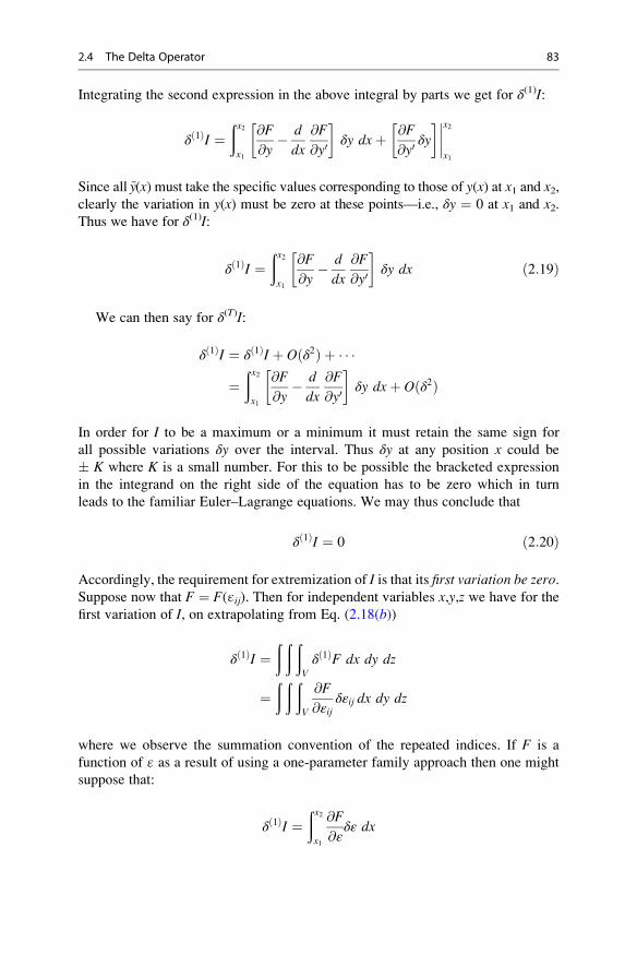
Integrating the second expression in the above integral by parts we get for δ(1)I:

δð1ÞI ¼ðx2x1

@F

@y� d

dx

@F

@y0

�δy dxþ @F

@y0δy

�x2

x1

Since all ~y(x) must take the specific values corresponding to those of y(x) at x1 and x2,clearly the variation in y(x) must be zero at these points—i.e., δy ¼ 0 at x1 and x2.Thus we have for δ(1)I:

δð1ÞI ¼ðx2x1

@F

@y� d

dx

@F

@y0

�δy dx ð2:19Þ

We can then say for δ(T)I:

δð1ÞI ¼ δð1ÞI þ Oðδ2Þ þ � � �

¼ðx2x1

@F

@y� d

dx

@F

@y0

�δy dxþ Oðδ2Þ

In order for I to be a maximum or a minimum it must retain the same sign for

all possible variations δy over the interval. Thus δy at any position x could be

� K where K is a small number. For this to be possible the bracketed expression

in the integrand on the right side of the equation has to be zero which in turn

leads to the familiar Euler–Lagrange equations. We may thus conclude that

δð1ÞI ¼ 0 ð2:20Þ

Accordingly, the requirement for extremization of I is that its first variation be zero.Suppose now that F ¼ F(ɛij). Then for independent variables x,y,z we have for thefirst variation of I, on extrapolating from Eq. (2.18(b))

δð1ÞI ¼ð ð ð

V

δð1ÞF dx dy dz

¼ð ð ð

V

@F

@εijδεij dx dy dz

where we observe the summation convention of the repeated indices. If F is a

function of ɛ as a result of using a one-parameter family approach then one might

suppose that:

δð1ÞI ¼ðx2x1

@F

@εδε dx

2.4 The Delta Operator 83

But the dependent variable represents the extremal function in the development,

and for the one-parameter development ɛ ¼ 0 corresponds to this condition.

Hence we must compute ∂F/∂ɛ at ɛ ¼ 0 in the above formulation and δɛ can

be taken as ɛ itself. Hence we get:

δð1ÞI ¼ðx1x2

@ ~F

@ε

� �ε¼0

ε dx ð2:21Þ

If we use a two-parameter family (as we soon shall) then it should be clear

for ɛ1 and ɛ2 as parameters that:

δð1ÞI ¼ðx2x1

@ ~F

@ε1

� �ε1 ¼ 0ε2 ¼ 0

ε1 þ @ ~F

@ε2

� �ε1 ¼ 0ε2 ¼ 0

ε2

24

35 dx ð2:22Þ

Now going back to Eq. (2.12) and its development we can say:

d~I

dε

� �ε¼0

¼ðx2x1

@F

@y� d

dx

@F

@y0

� � �η dx ð2:23Þ

Next rewriting Eq. (2.19) we have:

δð1ÞI ¼ðx2x1

@F

@y� d

dx

@F

@y0

� � �δy dx

Noting that δy ¼ ɛη for a single-parameter family approach we see by comparing

the right sides of the above equations that:

δð1ÞI � d~I

dε

� �ε ¼ 0

ε ð2:24Þ

Accordingly setting (d~I/dɛ)ɛ¼ 0 ¼ 0, as we have done for a single-parameter family

approach, is tantamount to setting the first variation of I equal to zero.9 We shall use

both approaches in this text for finding the extremal functions.

As a next step, we examine certain simple cases of the Euler–Lagrange equation

to ascertain first integrals.

9Note that for a two parameter family we have from Eq. (2.22) the result:

δð1ÞI ¼ @~I

@ε1

� �ε1 ¼ 0ε2 ¼ 0

ε1 þ @~I

@ε2

� �ε1 ¼ 0ε2 ¼ 0

ε2 ð2:25Þ


2.5 First Integrals of the Euler–Lagrange Equation

We now present four cases where we can make immediate statements concerning

first integrals of the Euler–Lagrange equation as presented thus far.

Case (a). F is not a function of y—i.e., F ¼ F(x, y0)In this case the Euler–Lagrange equation degenerates to the form:

d

dx

@F

@y0

� �¼ 0

Accordingly, we can say for a first integral that:

@F

@y0¼ Const: ð2:26Þ

Case (b). F is only a function of y0—i.e., F ¼ F(y0)Equation 2.26 still applies because of the lack of presence of the variable y.However, now we know that the left side must be a function only of y0. Sincethis function must equal a constant at all times we conclude that y0 ¼ const. is a

possible solution. This means that for this case an extremal path is simply that of

a straight line.

Case (c). F is independent of the independent variable x—i.e., F ¼ F(y, y0)For this case we begin by presenting an identity which you are urged to verify. Thus

noting that d/dx may be expressed here as

@

@xþ y0

@

@yþ y00

@

@y0

� �

we can say:

d

dxy0@F

@y0� F

� �¼ �y0

@F

@y� d

dx

@F

@y0

� � �� @F

@x

If F is not explicitly a function of x, we can drop the last term. A satisfaction of the

Euler–Lagrange equation now means that the right side of the equation is zero so

that we may conclude that

y0@F

@y0� F ¼ C1 ð2:27Þ

for the extremal function. We thus have next to solve a first-order differential

equation to determine the extremal function.

2.5 First Integrals of the Euler–Lagrange Equation 85

Case (d). Fis the total derivative of some functiong(x,y)—i.e., F ¼ dg/dxIt is easy to show that when F ¼ dg/dx, it must satisfy identically the

Euler–Lagrange equation. We first note that:

F ¼ @g

@xþ @g

@yy0 ð2:28Þ

Now substitute the above result into the Euler–Lagrange equation. We get:

@

@y

@g

@xþ @g

@yy0

� �� d

dx

@g

@y

� �¼ 0

Carry out the various differentiation processes:

@2g

@x @yþ @2g

@y2y0 � @2g

@x @y� @2g

@y2y0 ¼ 0

The left side is clearly identically zero and so we have shown that a suffi-cient condition for F to satisfy the Euler–Lagrange equation identically is that

F ¼ dg(x,y)/dx. It can also be shown that this is a necessary condition for the

identical satisfaction of the Euler–Lagrange equation. It is then obvious that we can

always add a term of the form dg/dx to the function F in I without changing

the Euler–Lagrange equations for the functional I. That is, for any Euler–Lagrange

equation there are an infinity of functionals differing from each other in theseintegrals by terms of the form dg/dx.

We shall have ample occasion to use these simple solutions. Now we consider

the geodesic problem, presented earlier, for the case of the sphere.

EXAMPLE 2.2. Consider a sphere of radius R having its center at the origin of

reference xyz. We wish to determine the shortest path between two points on

this sphere. Using spherical coordinates R, ϕ, E (see Fig. 2.4) a point P on the

sphere has the following coordinates:

x ¼ R sin θ cos ϕ

y ¼ R sin θ sin ϕ

z ¼ R cos θ

ðaÞ

The increment of distance ds on the sphere may be given as follows:

ds2 ¼ dx2 þ dy2 þ dz2 ¼ R2½dθ2 þ sin2θ dϕ2�

Hence the distance between point P and Q can be given as follows:

I ¼ðQP

ds ¼ðQP

R½dθ2 þ sin2 θ dϕ2�1=2 ðbÞ


With ϕ and θ as independent variables, the transformation equations (a) depicta sphere. If E is related to θ, i.e., it is a function of θ, then clearly x, y, and z inEq. (a) are functions of a single parameter θ and this must represent some curve on

the sphere. Accordingly, since we are seeking a curve on the sphere we shall assume

that ϕ is a function of θ in the above equation so that we can say:

I ¼ R

ðQP

1þ sin2θdϕ

dθ

� �2" #1=2

dθ ðcÞ

We have here a functional with θ as the independent variable and ϕ as the function,

with the derivative of ϕ appearing explicitly. With ϕ not appearing explicitly in the

integrand, we recognize this to be case (a) discussed earlier. We may then say,

using Eq. (2.26):

@

@ϕ0 ½1þ ðsin2θÞðϕ0Þ2�1=2 ¼ C1 ðdÞ

This becomes:

ðsin2θÞðϕ0Þ½1þ ðsin2θÞðϕ0Þ2�1=2

¼ C1

P

y

x

z

Rq

ø

Fig. 2.4

2.5 First Integrals of the Euler–Lagrange Equation 87

Solving for ϕ0 we get:

ϕ0 ¼ C1

sin θ½sin2θ � C12�1=2

Integrating we have:

ϕ ¼ C1

ðdθ

sin θ½sin2θ � C12�1=2

þ C2 ðeÞ

We make next the following substitution for θ:

θ ¼ tan�1 1

ηðf Þ

This gives us:

ϕ ¼ C1

ð 1

1þ η2dη

1

1þ η2

� �1=21

1þ η2� C2

1

�1=2 þ C2

¼ð

dη

1

C21

� 1

� �� η2

�1=2 þ C2

Denoting (1/C12 � 1)1/2 as 1/C3 we get on integrating:

ϕ ¼ sin�1ðC3ηÞ þ C2 ðgÞ

Replacing η from Eq. (f) we get:

ϕ ¼ sin�1 C3

1

tan θ

�þ C2

Hence we can say:

sinðϕ� C2Þ ¼ C3

tan θ

This equation may next be written as follows:

sin ϕ cos C2 � cos ϕ sin C2 ¼ C3

cos θ

sin θ


Hence:

sin ϕ sin θ cos C2 � sin θ cos ϕ sin C2 ¼ cos θ

Observing the transformation equations (a) we may express the above equation in

terms of Cartesian coordinates in the following manner:

y cos C2 � x sin C2 ¼ zC3 ðhÞ

wherein we have cancelled the term R. This is the equation of a plane surface goingthrough the origin. The intersection of this plane surface and the sphere then gives

the proper locus of points on the sphere that forms the desired extremal path.

Clearly this curve is the expected great circle. ////

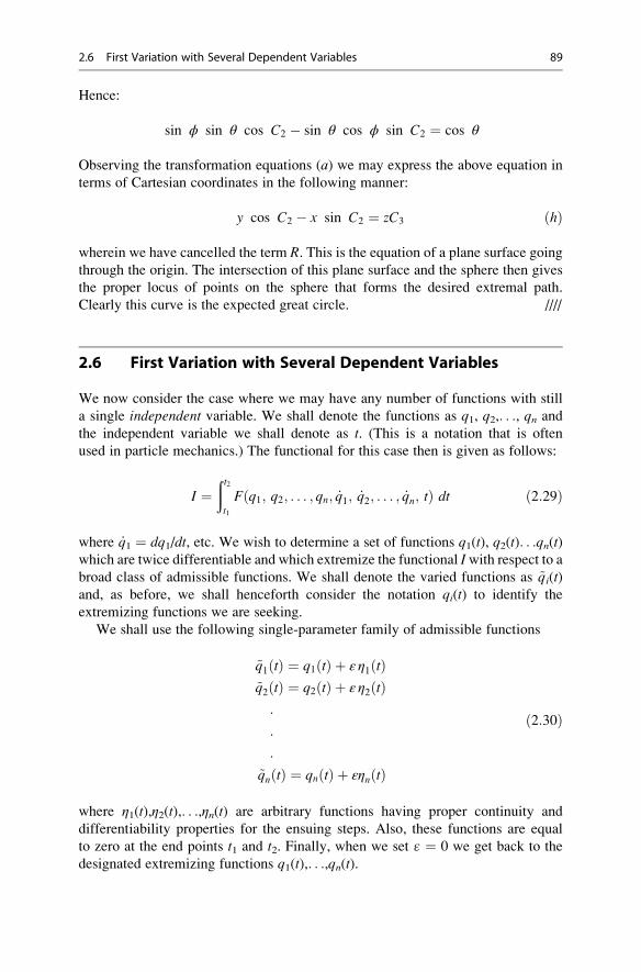
2.6 First Variation with Several Dependent Variables

We now consider the case where we may have any number of functions with still

a single independent variable. We shall denote the functions as q1, q2,. . ., qn andthe independent variable we shall denote as t. (This is a notation that is often

used in particle mechanics.) The functional for this case then is given as follows:

I ¼ðt2t1

Fðq1; q2; . . . ; qn; _q1; _q2; . . . ; _qn; tÞ dt ð2:29Þ

where _q1 ¼ dq1/dt, etc. We wish to determine a set of functions q1(t), q2(t). . .qn(t)which are twice differentiable and which extremize the functional Iwith respect to abroad class of admissible functions. We shall denote the varied functions as ~qi(t)and, as before, we shall henceforth consider the notation qi(t) to identify the

extremizing functions we are seeking.

We shall use the following single-parameter family of admissible functions

~q1ðtÞ ¼ q1ðtÞ þ ε η1ðtÞ~q2ðtÞ ¼ q2ðtÞ þ ε η2ðtÞ:

:

:

~qnðtÞ ¼ qnðtÞ þ εηnðtÞ

ð2:30Þ

where η1(t),η2(t),. . .,ηn(t) are arbitrary functions having proper continuity and

differentiability properties for the ensuing steps. Also, these functions are equal

to zero at the end points t1 and t2. Finally, when we set ɛ ¼ 0 we get back to the

designated extremizing functions q1(t),. . .,qn(t).

2.6 First Variation with Several Dependent Variables 89

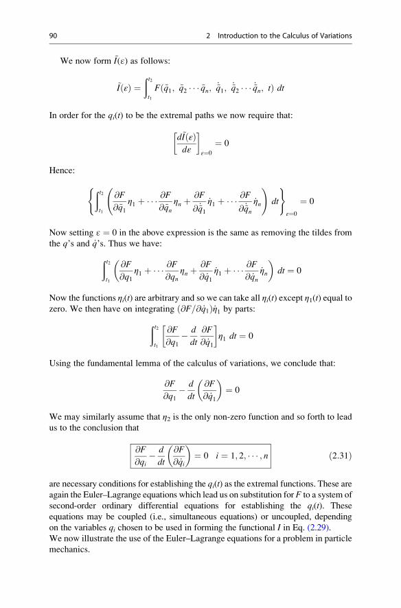
We now form ~I(ɛ) as follows:

~IðεÞ ¼ðt2t1

Fð~q1; ~q2 � � � ~qn; _~q1; _~q2 � � � _~qn; tÞ dt

In order for the qi(t) to be the extremal paths we now require that:

d~IðεÞdε

�ε¼0

¼ 0

Hence:

ðt2t1

@F

@~q1η1 þ � � � @F

@~qnηn þ

@F

@ _~q1_η1 þ � � � @F

@ _~qn_ηn

!dt

( )ε¼0

¼ 0

Now setting ɛ ¼ 0 in the above expression is the same as removing the tildes from

the q’s and _q’s. Thus we have:

ðt2t1

@F

@q1η1 þ � � � @F

@qnηn þ

@F

@ _q1_η1 þ � � � @F

@ _qn_ηn

� �dt ¼ 0

Now the functions ηi(t) are arbitrary and so we can take all ηi(t) except η1(t) equal tozero. We then have on integrating ð@F=@ _q1Þ _η1 by parts:

ðt2t1

@F

@q1� d

dt

@F

@ _q1

�η1 dt ¼ 0

Using the fundamental lemma of the calculus of variations, we conclude that:

@F

@q1� d

dt

@F

@ _q1

� �¼ 0

We may similarly assume that η2 is the only non-zero function and so forth to lead

us to the conclusion that

@F

@qi� d

dt

@F

@ _qi

� �¼ 0 i ¼ 1; 2; � � � ; n ð2:31Þ

are necessary conditions for establishing the qi(t) as the extremal functions. These are

again the Euler–Lagrange equations which lead us on substitution for F to a system of

second-order ordinary differential equations for establishing the qi(t). These

equations may be coupled (i.e., simultaneous equations) or uncoupled, depending

on the variables qi chosen to be used in forming the functional I in Eq. (2.29).

We now illustrate the use of the Euler–Lagrange equations for a problem in particle

mechanics.


EXAMPLE 2.3. We will present for use here the very important Hamilton principle

in order to illustrate the multi-function problem of this section. Later we shall take

the time to consider this principle in detail.

For a system of particles acted on by conservative forces, Hamilton’s principle

states that the proper paths taken from a configuration at time t1 to a configuration

at time t2 are those that extremize the following functional

I ¼ðt2t1

ðT � VÞ dt ðaÞ

where T is the kinetic energy of the system and therefore a function of velocity _xiof each particle while V is the potential energy of the system and therefore a

function of the coordinates xi of the particles. We thus have here a functional of

many dependent variables xi with the presence of a single independent variable, t.Consider two identical masses connected by three springs as has been shown in

Fig. 2.5. The masses can only move along a straight line as a result of frictionless

constraints. Two independent coordinates are needed to locate the system; they are

shown as x1 and x2. The springs are unstretched when x1 ¼ x2 ¼ 0.

From elementary mechanics we can say for the system:

T ¼ 1

2M _x1

2 þ 1

2M _x2

2

V ¼ 1

2K1x1

2 þ 1

2K2ðx2 � x1Þ2 þ 1

2K1x2

2 ðbÞ

Hence we have for I:

I ¼ðt2t1

1

2M _x1

2 þ _x22

� � 1

2K1x1

2 þ K2ðx2 � x1Þ2 þ K1x22

h i� �dt ðcÞ

x2x1

K1 K2 K1

MM

Fig. 2.5

2.6 First Variation with Several Dependent Variables 91

To extremize I we employ Eq. (2.31) as follows:

@F

@x1� d

dt

@F

@ _x1

� �¼ 0

@F

@x2� d

dt

@F

@ _x2

� �¼ 0 ðdÞ

Substituting we get:

� K1x1 þ K2ðx2 � x1Þ � d

dtðM _x1Þ ¼ 0

� K2x2 � K2ðx2 � x1Þ � d

dtðM _x2Þ ¼ 0 ðeÞ

Rearranging we then have:

M€x1 þ K1x1 � K2ðx2 � x1Þ ¼ 0

M€x2 þ K2x2 � K2ðx2 � x1Þ ¼ 0 ðf Þ

These are recognized immediately to be equations obtainable directly from

Newton’s laws. Thus the Euler–Lagrange equations lead to the basic equations of

motion for this case. We may integrate these equations and, using initial conditions

of _x1(0), _x2(0), x1(0) and x2(0), we may then fully establish the subsequent motion of

the system.

In this problem we could have more easily employed Newton’s law directly.

There are many problems, however, where it is easier to proceed by the variational

approach to arrive at the equations of motion. Also, as will be seen in the text, other

advantages accrue to the use of the variational method. ////

2.7 The Isoperimetric Problem

We now investigate the isoperimetric problem in its simplest form whereby we

wish to extremize the functional

I ¼ðx2x1

Fðx; y; y0Þ dx ð2:32Þ

subject to the restriction that y(x) have a form such that:

J ¼ðx2x1

Gðx; y; y0Þ dx¼ Const: ð2:33Þ

where G is a given function.

We proceed essentially as in Sec. 2.3. We take y(x) from here on to represent

the extremizing function for the functional of Eq. (2.32). We next introduce a


system of varied paths ~y(x) for computation of ~I. Our task is then to find conditions

required to be imposed on y(x) so as to extremize ~I with respect to the admissible

varied paths ~y (x) while satisfying the isoperimetric constraint of Eq. (2.33). To

facilitate the computations we shall require that the admissible varied paths also

satisfy Eq. (2.33). Thus we have:

~I ¼ðx2x1

Fðx; ~y; ~y0Þ dx ðaÞ

~J ¼ðx2x1

Gðx; ~y; ~y0Þ dx ¼ Const: ðbÞ

Because of this last condition on y(x) we shall no longer use the familiar single-

parameter family of admissible functions, since varying ɛ alone for a single

parameter family of functions may mean that the constraint for the corresponding

paths y(x) is not satisfied. To allow for enough flexibility to carry out extremization

while maintaining intact the constraining equations, we employ a two-parameter

family of admissible functions of the form,

~yðxÞ ¼ yðxÞ þ ε1η1ðxÞ þ ε2η2ðxÞ ð2:35Þ

where η1(x) and η2(x) are arbitrary functions which vanish at the end points x1, x2,and where ɛ1 and ɛ2 are two small parameters. Using this system of admissible

functions it is clear that ~I and ~J are functions of ɛ1 and ɛ2. Thus:

~I ε1; ε2ð Þ ¼ðx2x1

F x; ~y; ~y0ð Þ dx ðaÞ

~J ε1; ε2ð Þ ¼ðx2x1

G x; ~y; ~y0ð Þ dx ðbÞ

To extremize ~I when ~y ! y we require (see Eq. 2.25) that:

δð1Þ~I ¼ @~I

@ε1

� �ε1 ¼ 0ε2 ¼ 0

ε1 þ @~I

@ε2

� �ε1 ¼ 0ε2 ¼ 0

ε2 ¼ 0 ð2:37Þ

If ɛ1 and ɛ2 were independent of each other, we could then set each of the

partial derivatives in the above equation equal to zero separately to satisfy the

above equation. However, ɛ1 and ɛ2 are related by the requirement that ~J ( ɛ1, ɛ2)¼const. The first variation of ~Jmust be zero because of the constancy of its value and

we have the equation:

@ ~J

@ε1

� �ε1 ¼ 0ε2 ¼ 0

ε1 þ @ ~J

@ε2

� �ε1 ¼ 0ε2 ¼ 0

ε2 ¼ 0 ð2:38Þ

2.7 The Isoperimetric Problem 93

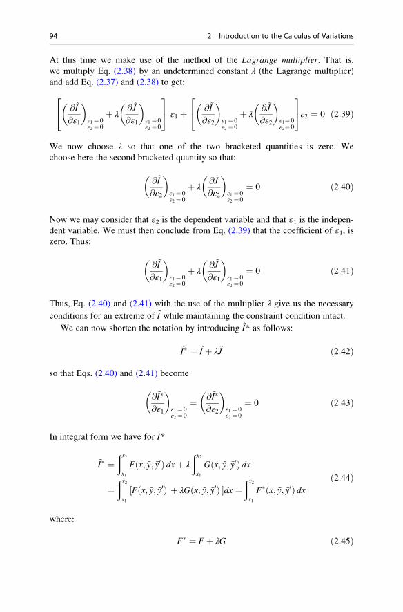
At this time we make use of the method of the Lagrange multiplier. That is,we multiply Eq. (2.38) by an undetermined constant λ (the Lagrange multiplier)

and add Eq. (2.37) and (2.38) to get:

@~I

@ε1

� �ε1 ¼ 0ε2 ¼ 0

þ λ@ ~J

@ε1

� �ε1 ¼ 0ε2 ¼ 0

24

35 ε1 þ @~I

@ε2

� �ε1 ¼ 0ε2 ¼ 0

þ λ@ ~J

@ε2

� �ε1¼ 0ε2¼ 0

24

35ε2 ¼ 0 ð2:39Þ

We now choose λ so that one of the two bracketed quantities is zero. We

choose here the second bracketed quantity so that:

@~I

@ε2

� �ε1 ¼ 0ε2 ¼ 0

þ λ@ ~J

@ε2

� �ε1 ¼ 0ε2 ¼ 0

¼ 0 ð2:40Þ

Now we may consider that ɛ2 is the dependent variable and that ɛ1 is the indepen-dent variable. We must then conclude from Eq. (2.39) that the coefficient of ɛ1, iszero. Thus:

@~I

@ε1

� �ε1 ¼ 0ε2 ¼ 0

þ λ@ ~J

@ε1

� �ε1 ¼ 0ε2 ¼ 0

¼ 0 ð2:41Þ

Thus, Eq. (2.40) and (2.41) with the use of the multiplier λ give us the necessary

conditions for an extreme of ~I while maintaining the constraint condition intact.

We can now shorten the notation by introducing ~I* as follows:

~I� ¼ ~I þ λ~J ð2:42Þ

so that Eqs. (2.40) and (2.41) become

@~I�

@ε1

� �ε1 ¼ 0ε2 ¼ 0

¼ @~I�

@ε2

� �ε1 ¼ 0ε2 ¼ 0

¼ 0 ð2:43Þ

In integral form we have for ~I*

~I� ¼ðx2x1

Fðx; ~y; ~y0Þ dxþ λ

ðx2x1

Gðx; ~y; ~y0Þ dx

¼ðx2x1

Fðx; ~y; ~y0Þ þ λGðx; ~y; ~y0Þ½ �dx ¼ðx2x1

F�ðx; ~y; ~y0Þ dxð2:44Þ

where:

F� ¼ Fþ λG ð2:45Þ


We now apply the conditions given by Eq. (2.43) using Eq. (2.44) to replace ~I*.

@~I�

@εi

� �ε1 ¼ 0ε2 ¼ 0

¼ðx2x1

@F�

@~yηi þ

@F�

@~y0η0i

� �dx

� �ε1 ¼ 0ε2 ¼ 0

¼ 0 i ¼ 1; 2 ð2:46Þ

We thus get a statement of the extremization process without the appearance of

the constraint and this now becomes the starting point of the extremization

process. Removing the tildes from ~y and ~y0 is equivalent to setting ɛi ¼ 0 and so

we may say:

@~I�

@εi

� �ε1 ¼ 0ε2 ¼ 0

¼ðx2x1

@F�

@yηi þ

@F�

@y0η0i

� �dx ¼ 0 i ¼ 1; 2 ð2:47Þ

Integrating the second expression in the integrand by parts and noting that ηi(x1) ¼ηi(x2) ¼ 0 we get:

ðx2x1

@F�

@y� d

dx

@F�

@y0

� �ηi dx ¼ 0 i ¼ 1; 2

Now using the fundamental lemma of the calculus of variations we conclude that:

@F�

@y� d

dx

@F�

@y0

� �¼ 0 ð2:48Þ

Thus the Euler–Lagrange equation is again a necessary condition for the desired

extremum, this time applied to F* and thus including the Lagrange multiplier.

This leads to a second-order differential equation for y(x), the extremizing function.

Integrating this equation then leaves us two constants of integration plus the

Lagrange multiplier. These are determined from the specified values of y at the

end points plus the constraint condition given by Eq. (2.33).

We have thus far considered only a single constraining integral. If we have “n”such integrals ðx2

x1

Gk x; y; y0ð Þdx ¼ Ck k ¼ 1; 2; � � � ; n

then by using an nþ 1 parameter family of varied paths ~y¼ yþ ɛ1η1þ ɛ2η2þ ··· ɛnþ1ηnþ 1 we can arrive as before at the following requirement for extremization:

@F�

@y� d

dt

@F�

@y0

� �¼ 0

2.7 The Isoperimetric Problem 95

where:

F� ¼ FþXnk¼1

λkGk

The λ’s are again the Lagrange multipliers. Finally, for p dependent variables, i.e.,

I ¼ðt2t1

F q1; q2; . . . ; qp; _q1; . . . ; _qp; t�

dt

with n constraints

ðt2t1

Gk q1; . . . ; qp; _q1; . . . ; _qp; t�

dt ¼ Ck k ¼ 1; 2; . . . ; n

the extremizing process yields

@F�

@qi� d

dt

@F�

@qi

� �¼ 0 i ¼ 1; . . . ; p ð2:49Þ

where

F� ¼ FþXn1

λkGk ð2:50Þ

We now illustrate the use of these equations by considering in detail the

isoperimetric problem presented earlier.

EXAMPLE 2.4. Recall from Sec. 2.2 that the isoperimetric problem asks us to find

the particular curve y(x) which for a given length L encloses the largest area A.Expressed parametrically we have a functional with two functions y and x; theindependent variable is τ. Thus:

I ¼ A ¼ 1

2

ðτ2τ1

xdy

dτ� y

dx

dτ

� �dτ ðaÞ

The constraint relation is:

L ¼ðτ2τ1

ffiffiffiffiffiffiffiffiffiffiffiffiffiffiffiffiffiffiffiffiffiffiffiffiffiffiffiffiffiffiffiffiffidx

dτ

� �2

þ dy

dτ

� �2s

dτ ðbÞ

We now form F* for this case. Thus:

F� ¼ 12ðx _y� y _xÞ þ λð _x2 þ _y2Þ1=2


where we use the dot superscript to represent (d/dτ). We now set forth the Euler–

Lagrange equations:

_y

2� d

dτ� y

2þ λ _x

_x2 þ _y2� 1=2

" #¼ 0 ðcÞ

� _x

2� d

dτ

x

2þ λ _y

_x2 þ _y2� 1=2

" #¼ 0 ðdÞ

We next integrate Eqs. (c) and (d) with respect to τ to get:

y� λ _x

_x2 þ _y2� 1=2 ¼ C1 ðeÞ

xþ λ _y

_x2 þ _y2� 1=2 ¼ C2 ðf Þ

After eliminating λ between the equations we will reach the following result:

x� C2ð Þ dxþ y� C1ð Þdy ¼ 0ðgÞ ðgÞ

The last equation is easily integrated to yield:

ðx� C2Þ22

þ ðy� C1Þ22

¼ C32 ðhÞ

where C3 is a constant of integration. Thus we get as the required curve a circle—a

result which should surprise no one. The radius of the circle isffiffiffi2

pC3 which you may

readily show (by eliminating C1 and C2 from Eq. (h) using Eqs. (e) and (f) andsolving for λ) is the value of the Lagrange multiplier10 λ. The constants C1 and C2

merely position the circle. ////

2.8 Functional Constraints

We now consider the functional

I ¼ðt2t1

F q1; q2; . . . ; qn; _q1; . . . ; _qn; tð Þ dt ð2:51Þ

with the following m constraints on the n functions qi:11

10The Lagrange multiplier is usually of physical significance.11In dynamics of particles, if the constraining equations do not have derivatives the constraints are

called holomonic.

2.8 Functional Constraints 97

G1 q1; . . . ; qn; _q1; . . . ; _qn; tð Þ ¼ 0

..

.

Gm q1; . . . ; qn; _q1; . . . ; _qn; tð Þ ¼ 0

ð2:52Þ

We assume m < n. To extremize the functional I we may proceed by employing none-parameter families of varied functions of the form

~qiðtÞ ¼ qiðtÞ þ εηiðtÞ i ¼ 1; . . . ; n ð2:53Þ

where ηi(t1) ¼ ηi(t2) ¼ 0. Furthermore we assume that the varied functions ~qisatisfy the constraining equation (2.52). That is,

Gj ~q1; . . . ; ~qn; _~q1; . . . ; _~qn; t� ¼ 0 j ¼ 1; . . .m ð2:54Þ

We now set the first variation of I equal to zero.

δ 1ð ÞI ¼ 0 ¼ @~I

@ε

� �ε¼0

ε

Setting (∂ ~I/∂ɛ)ɛ¼ 0 equal to zero we have:

ðt2t1

@F

@~q1η1 þ � � � þ @F

@~qnηn þ

@F

@ _~q1_η1 þ � � � þ @F

@ _~qn_ηn

" #dt

" #ε¼ 0

¼ 0

Dropping the tildes and subscript ɛ ¼ 0 we have:

ðt2t1

@F

@q1η1 þ � � � þ @F

@qnηn þ

@F

@ _q1_η1 þ � � � þ @F

@ _qn_ηn

� �dt ¼ 0 ð2:55Þ

Since the varied q’s satisfy the constraining equations, by assumption, we can

conclude since Gi ¼ 0 that:

δð1Þ Gið Þ ¼ 0 ¼ @G

@ε

� �ε ¼ 0

ε

Setting (∂Gi/∂ɛ)ɛ¼ 0 ¼ 0 here we have:

@Gi

@~q1η1 þ � � � þ @Gi

@ _~q1ηn þ

@Gi

@ _~q1_η1 þ � � � þ @Gi

@ _~qn_ηn

( )ε¼ 0

¼ 0

i ¼ 1; 2; . . . ;m


Dropping the tildes and ɛ ¼ 0 we then have:

@Gi

@q1η1 þ � � � þ @Gi

@qnηn þ

@Gi

@ _q1_η1 þ � � � þ @Gi

@ _qn_ηn ¼ 0 i ¼ 1; . . . ;m

We now multiply each of the above m equations by an arbitrary time function, λi(t),which we may call a Lagrange multiplier function. Adding the resulting equations

we have:

Xmi¼1

λi tð Þ @Gi

@q1η1 þ � � � þ @Gi

@qnηn þ

@Gi

@ _q1_η1 þ � � � þ @Gi

@ _qn_η

�¼ 0

Now integrate the above sum from t1 to t2 and then add the results to Eq. (2.55). We

then have:

ðt2t1

@F

@q1η1 þ � � � þ @F

@qnηn þ

@F

@ _q1_η1 þ � � � þ @F

@ _qn_ηn

�

þXmi¼ 1

λi@Gi

@q1η1 þ � � � þ @Gi

@qnηn þ

@Gi

@ _q1_η1 þ � � � þ @Gi

@ _qn_ηn

� �)dt ¼ 0

Integrating by parts the terms with _ηi and regrouping the results we then have:

ðt2t1

@F

@q1� d

dt

@F

@ _q1

� �þXmi¼1

λi@Gi

@q1� d

dtλi@Gi

@ _q1

� � �( )" #η1

þ � � � � � � � � � � � � � � � � � � � � � � � � � � � � � � � � � � � � � � � � � � � � � � � � �þ � � � � � � � � � � � � � � � � � � � � � � � � � � � � � � � � � � � � � � � � � � � � � � � � �

þ @F

@qn� d

dt

@F

@ _qn

� �þXmi¼ 1

λi@Gi

@qn� d

dtλi@Gi

@ _qn

� � �( )ηn

#dt ¼ 0 ð2:56Þ

Now introduce F* defined as:

F� ¼ FþXmi¼ 1

λi tð ÞGi ð2:57Þ

We can then rewrite Eq. (2.56) as follows:

ðt2t1

@F�

@q1� d

dt

@F�

@ _q1

� �η1 þ � � � þ @F�

@qn� d

dt

@F�

@ _qn

� �ηn

� �dt ¼ 0

2.8 Functional Constraints 99

Now the η’s are not independent (they are related through m equations (2.54))

and so we cannot set the coefficients of the bracketed expressions equal to zero

separately. However, we can say that (n � m) of the η’s are independent. For

the remaining m η’s we now assume that the time functions λi(t) are so chosen

that the coefficients of the η’s are zero. Then, since we are left with only

independent η’s, we can take the remaining coefficients equal to zero. In this

way we conclude that:

@F�

@qi� d

dt

@F�

@ _q1¼ 0 i ¼ 1; 2; � � � ; n

We thus arrive at the Euler–Lagrange equations once again. However, we have now

m unknown time functions λi to be determined with the aid of the original mconstraining equations.

We shall have ample opportunity of using the formulations of this section in

the following chapter when we consider the Reissner functional.

2.9 A Note on Boundary Conditions

In previous efforts at extremizing I we specified the end points (x1, y1) and (x2, y2)through which the extremizing function had to proceed. Thus, in Fig. 2.2 we asked

for the function y(x) going through (x1, y1) and (x2, y2) to make it extremize Irelative to neighboring varied paths also going through the aforestated end points.

The boundary conditions specifying y at x1 and at x2 are called the kinematic or

rigid boundary conditions of the problem.

We now pose a different query. Suppose only x1 and x2 are given as has been

shown in Fig. 2.6 and we ask what is the function y(x) that extremizes the functionalÐ x2x1F x; y; y0ð Þ dx between these limits. Thus, we do not specify y at x1 and x2 for the

extremizing function.

As before, we denote the extremizing function in the discussion as y(x) and we

have shown it so labeled at some position in Fig. 2.6. A system of nearby admissible

“paths” ~y(x) has also been shown. Some of these paths go through the endpoints of

the extremizing path while others do not. We shall extremize I with respect to such

a family of admissible functions to obtain certain necessary requirements for y(x) tomaintain the role of the extremizing function. Thus with the δ operator we arrive atthe following necessary condition using the same steps of earlier discussions and

noting that δy need no longer always be zero at the end points:

δð1ÞI ¼ 0 ¼ðx2x1

@F

@y� d

dx

@F

@y0

� � �δy dxþ @F

@y0δy

x¼x1

� @F

@y0δy

x¼x2

ð2:58Þ


There are admissible functions that go through the end points (x1, y1) and (x2, y2) ofthe designated extremizing function y(x). For such admissible functions δy1¼ δy2¼0 and we conclude that a necessary condition for an extremum is:

ðx2x1

@F

@y� d

dx

@F

@y0

� � �δy dx ¼ 0

Following the familiar procedures of previous computations we readily then arrive at

the Euler–Lagrange equations as a necessary condition for y(x) to be an extreme:

@F

@y� d

dx

@F

@y0

� �¼ 0

There are now, however, additional necessary requirements for extremizing I if δyis not zero at the end points of the extremizing function. Accordingly from

Eq. (2.58) we conclude that for such circumstances we require:

@F

@y0

x¼x1

¼ 0 að Þ

@F

@y0

x¼x2

¼ 0 bð Þ

The conditions (2.59) are termed the natural boundary conditions. They are the

boundary conditions that must be prescribed if both the values y(x1) and y(x2) arenot specified.12 However, it is also possible to assign one natural and one kinematic

boundary condition to satisfy the requirements for y(x) to fulfill its assigned role as

x1 x2

x

y

y1

y2

y

y

y

Fig. 2.6

12In problems of solid mechanics dealing with the total potential energy we will see that the

kinematic boundary conditions involve displacement conditions of the boundary while natural

boundary conditions involve force conditions at the boundary.

2.9 A Note on Boundary Conditions 101

extremizing function. In more general functionals I set forth earlier and those to be

considered in following sections, we find natural boundary conditions in much the

same way as set forth in this section. In essence we proceed with the variation

process without requiring the η functions (or by the same token the variations δy) tobe zero at the boundaries. Rather we set equal to zero all expressions established on

the boundary by the integration by parts procedures. The resulting conditions are

the natural boundary conditions.

Note that for all various possible boundary conditions, we work in any particular

case with the same differential equation. However, the extremal function will even-

tually depend on the particular permissible combination of boundary conditions

we choose to employ. Usually certain kinematic boundary conditions are imposed

by the constraints present in a particular problem. We must use these boundary

conditions or else our extremal functions will not correspond to the problem at

hand. The remaining boundary conditions then are natural ones that satisfy the

requirements for the extremizing process. We shall illustrate these remarks in

Example 2.5 after a discussion of higher-order derivatives.

2.10 Functionals Involving Higher-Order Derivatives

We have thus far considered only first-order derivatives in the functionals. At this

time we extend the work by finding extremal functions y(x) for functionals havinghigher-order derivatives. Accordingly we shall consider the following functional:

I ¼ðx2x1

F x; y; y0; y00; y000ð Þdx ð2:60Þ

The cases for lower or higher-order derivatives other than y000 are easily attainable

from the procedure that we shall follow. Using the familiar one-parameter family of

admissible functions for extremizing I we can then say:

d~I

dε

� �ε¼ 0

¼ d

dε

ðx2x1

F x; ~y; ~y0; ~y00; ~y000ð Þdx �

ε¼ 0

¼ 0

This becomes:

ðx2x1

@F

@~yηþ @F

@~y0η0 þ @F

@~y00η00 þ @F

@~y000η000

�dx

� �ε¼0

¼ 0

We may drop the subscript ɛ ¼ 0 along with the tildes as follows:

ðx2x1

@F

@yηþ @F

@y0η0 þ @F

@y00η00 þ @F

@y000η000

�dx ¼ 0


We now carry out the following series of integration by parts:

ðx2x1

@F

@y0η0dx ¼ @F

@y0η

x2

x1

�ðx2x1

d

dx

@F

@y0

�η dx

ðx2x1

@F

@y00η00dx ¼ @F

@y00η0x2

x1

�ðx2x1

d

dx

@F

@y00

�η0 dx

¼ @F

@y00η0x2

x1

� d

dx

@F

@y00

� �η

x2

x1

þðx2x1

d2

dx2@F

@y00

� �η dx

ðx2x1

@F

@y000η000dx ¼ @F

@y000η00x2

x1

�ðx2x1

d

dx

@F

@y000

�η00 dx

¼ @F

@y000η00x2

x1

� d

dx

@F

@y000

� �η0x2

x1

þðx2x1

d2

dx2@F

@y000

� �η0 dx

¼ @F

@y000η00x2

x1

� d

dx

@F

@y000

� �η0x2

x1

þ d2

dx2@F

@y000

� �η

x2

x1

�ðd3

dx3@F

@y000

� �η dx

Now combining the results we get:

�ðx2x1

d3

dx3@F

@y000

� �� d2

dx2@F

@y00

� �þ d

dx

@F

@y0

� �� @F

@y

�η dx

þ @F

@y000η00x2

x1

� d

dx

@F

@y000� @F

@y00

� �η0x2

x1

þ d2

dx2@F

@y000

� �� d

dx

@F

@y00

� �þ @F

@y0

� �η

x2

x1

¼ 0 ð2:61Þ

Since the function η having the properties such that η(x1) ¼ η0(x1) ¼ η00(x1) ¼η(x2) ¼ η0(x2) ¼ η00(x2) ¼ 0 are admissible no matter what the boundary conditions

may be, it is clear that a necessary condition for an extremum is:

ðx2x1

d3

dx3@F

@y000

� �� d2

dx2@F

@y00

� �þ d

dx

@F

@y0

� �� @F

@y

�η dx ¼ 0

And we can then arrive at the following Euler–Lagrange equation:

d3

dx3@F

@y000

� �� d2

dx2@F

@y00

� �þ d

dx

@F

@y0

� �� @F

@y¼ 0 ð2:62Þ

2.10 Functionals Involving Higher-Order Derivatives 103

If, specifically, the conditions y(x1), y(x2), y0(x1), y0(x2), y00(x1) and y00(x2) are

specified (these are the kinematic boundary conditions of this problem), the admis-

sible functions must have these prescribed values and these prescribed derivatives

at the end points. Then clearly we have for this case:

η x1ð Þ ¼ η x2ð Þ ¼ η0 x1ð Þ ¼ η0 x2ð Þ ¼ η00 x1ð Þ ¼ η00 x2ð Þ ¼ 0

Thus we see that giving the kinematic end conditions and satisfying the

Euler–Lagrange equations permits the resulting y(x) to be an extremal. If the

kinematic conditions are not specified then we may satisfy the natural boundaryconditions for this problem. Summarizing, we may use either of the following

overall sets of requirements (see Eq. (2.61)) at the end points:

Kinematic Natural

y00 specified or@F

@y000¼ 0 ðaÞ

y0 specified ord

dx

@F

@y000

� �� @F

@y00¼ 0 ðbÞ

y specified ord2

dx2@F

@y000

� �� d

dx

@F

@y00

� �þ @F

@y0¼ 0 ðcÞ ð2:63Þ

Clearly combinations of kinematic and natural boundary conditions are also

permissible.

It should be apparent that by disregarding the terms involving y000 we may use the

results for a functional whose highest-order derivative is second-order. And, by

disregarding both terms with y000 and with y00, we get back to the familiar

expressions used earlier where y0 was the highest-order term in the functional.

Furthermore the pattern of growth from first order derivatives on up is clearly

established by the results so that one can readily extrapolate the formulations for

orders higher than three. Finally we may directly extend the results of this

problem to include function I with more than one function y. We simply get

equations of the form (2.62) for each function. Thus for t as the independent

variable and q1, q2,. . ., qn as the functions in I we have for derivatives up to order

three for all functions:

d3

dt3@F

@q0001

� �� d2

dt2@F

@q001

� �þ d

dt

@F

@q01

� �� @F

@q1¼ 0

..

.

d3

dt3@F

@q000n

� �� d2

dt2@F

@q00n

� �þ d

dt

@F

@q0n

� �� @F

@qn¼ 0

Similarly for each q we have a set of conditions corresponding to Eq. (2.63).


EXAMPLE 2.5. We now consider the deflection w of the centerline of a simply-

supported beam having a rectangular cross section and loaded in the plane of

symmetry of the cross section (see Fig. 2.7). In Chap. 4 we will show through

the principal of minimum total potential energy that the following functional is to

be extremized in order to insure equilibrium:

I ¼ðL0

EI

2

d2w

dx2

� �2

� qw

" #dx ðaÞ

where I is the second moment of the cross section about the horizontal centroidal

axis, and q is the transverse loading function.

The Euler–Lagrange equation for this case may be formed from Eq. (2.62) as

follows:

� d2

dx2@F

@w00

� �þ d

dx

@F

@w0� �

� @F

@w¼ 0 ðbÞ

where

F ¼ EI

2ðw00Þ2 � qw ðcÞ

We then get for the Euler–Lagrange equation:

� d2

dx2EIw00ð Þ þ d

dxð0Þ þ q ¼ 0

w(x)

q(x)

x

L

w

Fig. 2.7

2.10 Functionals Involving Higher-Order Derivatives 105

http://dx.doi.org/10.1007/272937_4

therefore

EIwIV ¼ q ðdÞ

The possible boundary conditions needed for extremization of functional (a) can bereadily deduced from Eq. (2.63). Thus at the end points:

w0 specified or@F

@w00 ¼ 0 ðeÞ

w specified or� d

dx

@F

@w00

� �þ @F

@w0 ¼ 0 ðf Þ

It is clear from Fig. 2.7 that we must employ the kinematic boundary condition w¼0 at the ends. In order then to carry out the extremization process properly we must

require additionally that:

@F

@w00 ¼ 0 at ends ðgÞ

Substituting for F we get:

w00ð0Þ ¼ w00ðLÞ ¼ 0 ðhÞ

You may recall that this indicates that the bending moments are zero at the ends—a

condition needed for the frictionless pins there. We thus see here that the natural

boundary conditions have to do with forces in structural problems. ////

In the following section we consider the case where we have higher-order

derivatives involving more than one independent variable.

2.11 A Further Extension

As we shall demonstrate later, the total potential energy in a plate is generally

expressible as a double integral of the displacement function w and partial

derivatives of w in the following form:

I ¼ð ð

S

F x; y;w;@w

@x;@w

@y;@2w

@x2;@2w

@x @y;@2w

@y @x;@2w

@y2

� �dx dy ð2:65Þ

where S is the area over which the integration is carried out. Using the notation

∂w/∂x ¼ wx, ∂2w/∂x2 ¼ wxx, etc., the above functional may be given as follows:


I ¼ð ð

S

F x; y;w;wx;wy;wxy;wyx;wyy;wxx

� dx dy ð2:66Þ

We have here a functional with more than one independent variable. The

procedure for finding the extremizing function, which we consider now to be

represented as w(x,y) is very similar to what we have done in the past. We use

as admissible functions, ~w (x,y), a one parameter family of functions defined

as follows:

~wðx; yÞ ¼ wðx; yÞ þ ε ηðx; yÞ ð2:67Þ

Accordingly we have for the extremization process:

d~I

dε

� �ε¼0

¼ 0 ¼ð ð

S

@F

@ ~wη

�þ @F

@ ~wxηx þ

@F

@ ~wyηy þ

@F

@ ~wxxηxx þ

@F

@ ~wxyηxy

�

þ @F

@ ~wyxηyx þ

@F

@ ~wyyηyy

�dx dy

�ε¼ 0

We may remove the tildes and the subscript notation ɛ¼ 0 simultaneously to get the

following statement:

ð ðS

@F

@wηþ @F

@wxηx þ

@F

@wyηy þ

@F

@wxx

ηxx

þ @F

@wxyηxy þ

@F

@wyxηyx þ

@F

@wyyηyy

�dx dy ¼ 0 ð2:68Þ

The familiar integration by parts process can be carried out here by employing

Green’s theorem (see Appendix I) in two dimensions which is given as follows:

ð ðS

G@η

@xdx dy ¼ �

ð ðS

@G

@xη dx dyþ

þηG cos ðn; xÞ dl ð2:69Þ

Recall that n is the normal to the bounding curve C of the domain S. We apply the

above theorem once to the second and third terms in the integrand of Eq. (2.68) and

twice to the last four terms to get:

ð ðS

@F

@w� @

@x

@F

@wx

� �� @

@y

@F

@wy

� �þ @2

@x2@F

@wxx

� �

þ @2

@x @y

@F

@wxy

� �þ @2

@y @x

@F

@wyx

� �þ @2

@y2@F

@wyy

� ��η dx dy

þ System of Line Integrals ¼ 0

2.11 A Further Extension 107

We can conclude, as in earlier cases, that a necessary requirement is that:

@F

@w� @

@x

@F

@wx

� �� @

@y

@F

@wy

� �þ @2

@x2@F

@wxx

� �

þ @2

@y @x

@F

@wyx

� �þ @2

@x @y

@F

@wxy

� �þ @2

@y2@F

@wyy

� �¼ 0 ð2:70Þ

This is the Euler–Lagrange equation for this case. We may deduce the natural

boundary conditions from the line integrals. However, we shall exemplify this step

later when we study the particular problem of classical plate theory, since the

results require considerable discussion.

If we have several functions in F, we find that additional equations of the form

given by Eq. (2.70) then constitute additional Euler–Lagrange equations for the

problem.

2.12 Closure

We have set forth a brief introduction in this chapter into elements of the calculus of

variations. In short, we have considered certain classes of functionals with the view

toward establishing necessary conditions for finding functions that extremize the

functionals. The results were ordinary or partial differential equations for the

extremizing functions (the Euler–Lagrange equations) as well as the establishment

of the dualities of kinematic (or rigid) and natural boundary conditions. We will see

later that the natural boundary conditions are not easily established without the use

of the variational approach. And since these conditions are often important for

properly posing particular boundary value problems, we can then conclude that the

natural boundary conditions are valuable products of the variational approach.

We also note that by the nature of the assumption leading to Eq. (2.9) we have

been concerned with varied paths, ~y(x), which not only are close to the extremal y(x)but which have derivatives ~y 0(x) close to y0(x). Such variations are called weakvariations. There are, however, variations which do not require the closeness of thederivatives of the varied paths to that of the extremal function (see Fig. 2.8 showing

such a varied path). When this is the case we say that we have strong variations. Amore complex theory is then needed beyond the level of this text. The reader is

referred to more advanced books such as those given in the footnote on page 71.

In the remainder of the text we shall employ the formulations presented in this

chapter for Euler–Lagrange equations and boundary conditions when there is only a

single independent variable present. The equations, you should recall, are then

ordinary differential equations and the boundary conditions are prescriptions at end

points. For more than one independent variable, we shall work out the

Euler–Lagrange equations (now partial differential equations) as well as the bound-

ary conditions (now line or surface integrals) from first principles using the formu-

lation δ(1)(I) ¼ 0 or (∂ ~I/∂ ɛ)ɛ ¼ 0 ¼ 0 as the basis of evaluations.


It is to be pointed out that this chapter does not terminate the development of the

calculus of variations. In the later chapters we shall investigate the process of going

from a boundary value problem to a functional for which the differential equation

corresponds to the Euler–Lagrange equations. This is inverse to the process set forth

in this chapter and leads to the useful quadratic functional. In Chap. 7 we shall set

forth two basic theorems, namely the maximum theorem and the “mini-max”

theorem which form the basis for key approximation procedures used for estimating

eigenvalues needed in the study of vibrations and stability of elastic bodies.

Additionally, in Chap. 9 we shall examine the second variation. Clearly there will

be a continued development of the calculus of variations as we proceed.

Our immediate task in Chap. 3 is to set forth functionals whose Euler–Lagrange

equation and boundary conditions form important boundary value problems in solid

mechanics. We shall illustrate the use of such functionals for problems of simple

trusses; we thus launch the study of structural mechanics as a by-product. Additionally

we shall introduce certain valuable approximation techniques associated with the

variational process that form the cornerstone of much such work throughout the text.

It may be apparent from these remarks that Chap. 3 is one of the key chapters in

this text.

Problems

2.1 Given the functional:

I ¼ðx2x1

ð3x2 þ 2xðy0Þ2 þ 10xyÞdx

What is the Euler–Lagrange equation?

y(x)

y(x) y(x)

y' (x) ≅ y' (x)

x

y(x)

Strong varaiations

˜

˜

˜

Fig. 2.8

Problems 109

http://dx.doi.org/10.1007/272937_7

http://dx.doi.org/10.1007/272937_9

http://dx.doi.org/10.1007/272937_3

http://dx.doi.org/10.1007/272937_3

2.2 What is the first variation of F in the preceding problem? What is the first

variation of I in this problem?

2.3 What is the Euler–Lagrange equation for the functional

I ¼ðx2x1

ð3x2 þ 2xy0 þ 10Þdx

2.4 Justify the identity given at the outset of Case (c) in Sec. 2.5.

2.5 Consider the functional:

I ¼ðx2x1

3ðy0Þ2 þ 4xh i

dx

What is the extremal function? Take y ¼ 0 at the end points.

2.6 Fermat’s principle states that the path of light is such as to minimize the time

passage from one point to another. What is the proper path of light in a plane

medium from point (1) to point (2) (Fig. 2.9) wherein the speed of light is

given as: (a) v ¼ Cy (b) v ¼ C/y?2.7 Demonstrate that the shortest distance between two points in a plane is a

straight line.

2.8 Consider a body of revolution moving with speed V through rarefied gas

outside the earth’s atmosphere (Fig. 2.10). We wish to design the shape of

the body, i.e., get y(x), so as to minimize the drag. Assume that there is no

friction on the body at contact with the molecules of the gas. Then one can

readily show that the pressure on the body is given as:

p ¼ 2ρV2 sin2 θ

(This means that the molecules are reflected specularly.) Show that the drag

FD for a length L of the body is given as:

FD ¼ðL0

4πρV2ðsin3θÞy 1þ dy

dx

� �2" #1=2

dx

Assume now that dy/dx is small so that

sin θ ¼ dy=dx

½1þ ðdy=dxÞ2�1=2ffi dy

dx

� �

Show that

FD ¼ 4πρV2

ðL0

dy

dx

� �3

y dx


What is the Euler–Lagrange equation for y(x) in order to minimize the

drag?

2.9 Consider the problem wherein a curve is desired between points (x1, y1) and(x2, y2) (see Fig. 2.11) which upon rotation about the x axis produces a

surface of revolution having a minimum area. Show that the solution is of

the form:

y ¼ C1 cosh t; t ¼ xþ C2

C1

which is the parametric representation of a catenary.2.10 Use the δ operator on the functional given in the text to find the

Euler–Lagrange equation for the brachistochrone problem.

1

y

2

x

Fig. 2.9

V

L

y

x

q

Fig. 2.10

Problems 111

2.11 Using Hamilton’s principle find the equations of motion for the system shown

in Fig. 2.12 for small oscillations.

2.12 Using Hamilton’s principle show that

ðmR2ϕ sin2θÞ ¼ Const:

for the spherical pendulum shown in Fig. 2.13. Gravity acts in the �z direc-tion. Neglect friction and the weight of the connecting link R. Use spherical

coordinates θ and ϕ as shown in the diagram and take the lowest position of mas the datum for potential energy.

2.13 Use the δ operator on the functional given in the text to find the

Euler–Lagrange equations for the spring-mass system in Example 2.3

K1 K2

M2

M1

L

a

Fig. 2.12

y

x

x2, y2x1, y1

Fig. 2.11


2.14 Extend the results of Problem 2.7 to any two points in three-dimensional

space.

2.15 Consider the case of a rope hanging between two points (x1,y1) and (x2,y2) asshown in Fig. 2.14. Find the Euler–Lagrange equation for the rope by

minimizing the potential energy of the rope for a given length L. The rope

is perfectly flexible. Show that

y ¼ �λ

gwþ C1

wgcosh

ðxþ C2ÞC1

How are C1, C2, and λ obtained?

w mass per unit length

x1 x2

x

y2

y1

yFig. 2.14

z

y

x

q

R

f

f

M R sin q

R

q = Const planeperpendicular view

xxy plane

z

Fig. 2.13

Problems 113

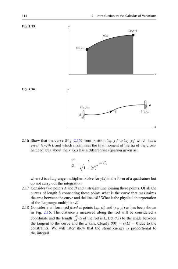
2.16 Show that the curve (Fig. 2.15) from position (x1, y1) to (x2, y2) which has agiven length L and which maximizes the first moment of inertia of the cross-

hatched area about the x axis has a differential equation given as:

y2

2þ λffiffiffiffiffiffiffiffiffiffiffiffiffiffiffiffiffiffi

1þ ðy0Þ2q ¼ C1

where λ is a Lagrange multiplier. Solve for y(x) in the form of a quadrature but

do not carry out the integration.

2.17 Consider two points A and B and a straight line joining these points. Of all the

curves of length L connecting these points what is the curve that maximizes

the area between the curve and the line AB?What is the physical interpretation

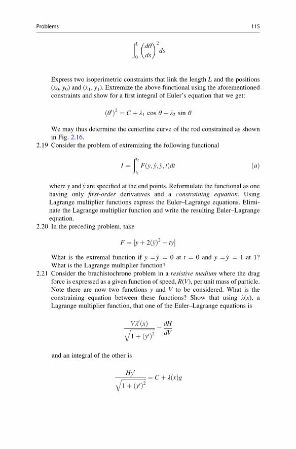
of the Lagrange multiplier λ?2.18 Consider a uniform rod fixed at points (x0, y0) and (x1, y1) as has been shown

in Fig. 2.16. The distance s measured along the rod will be considered a

coordinate and the lengthÐ BA ds of the rod is L. Let θ(s) be the angle between

the tangent to the curve and the x axis. Clearly θ(0) ¼ θ(L) ¼ 0 due to the

constraints. We will later show that the strain energy is proportional to

the integral.

y

AS

B

x

(x0 ,y0)(x1,y1)

Fig. 2.16

y

x

y(x)

(x1,y1)

(x2,y2)Fig. 2.15


ðL0

dθ

ds

� �2

ds

Express two isoperimetric constraints that link the length L and the positions

(x0, y0) and (x1, y1). Extremize the above functional using the aforementioned

constraints and show for a first integral of Euler’s equation that we get:

ðθ0Þ2 ¼ Cþ λ1 cos θ þ λ2 sin θ

We may thus determine the centerline curve of the rod constrained as shown

in Fig. 2.16.

2.19 Consider the problem of extremizing the following functional

I ¼ðt2t1

Fðy; _y; €y; tÞdt ðaÞ

where y and _y are specified at the end points. Reformulate the functional as one

having only first-order derivatives and a constraining equation. Using

Lagrange multiplier functions express the Euler–Lagrange equations. Elimi-

nate the Lagrange multiplier function and write the resulting Euler–Lagrange

equation.

2.20 In the preceding problem, take

F ¼ ½yþ 2ð€yÞ2 � ty�

What is the extremal function if y ¼ _y ¼ 0 at t ¼ 0 and y ¼ _y ¼ 1 at 1?

What is the Lagrange multiplier function?

2.21 Consider the brachistochrone problem in a resistive medium where the drag

force is expressed as a given function of speed, R(V), per unit mass of particle.

Note there are now two functions y and V to be considered. What is the

constraining equation between these functions? Show that using λ(x), a

Lagrange multiplier function, that one of the Euler–Lagrange equations is

Vλ0ðxÞffiffiffiffiffiffiffiffiffiffiffiffiffiffiffiffiffiffi1þ ðy0Þ2

q ¼ dH

dV

and an integral of the other is

Hy0ffiffiffiffiffiffiffiffiffiffiffiffiffiffiffiffiffiffi1þ ðy0Þ2

q ¼ Cþ λðxÞg

Problems 115

where C is a constant of integration, g is the acceleration of gravity, and H is

given as:

H ¼ 1

Vþ λðxÞRðVÞ

2.22 Derive the Euler–Lagrange equation and the natural boundary conditions for

the following functional:

I ¼ðx2x1

Fðx; d4y=dx4Þdx

2.23 Do Problem 2.19 using the given functional F (i.e., with second-order

derivative).

2.24 Derive the Euler–Lagrange equation and natural and geometric boundary

conditions of beam theory using the δ operator on the functional given in

the text (Example 2.5).

2.25 In our study of plates we will see (Chap. 6) that to find the equation of

equilibrium for a circular plate (see Fig. 2.17) loaded symmetrically by a

force per unit area q(r), and fixed at the edges, we must extremize the following

functional:

I ¼ Dπ

ða0

rd2w

dr2

� �2

þ 1

r

dw

dr

� �2

þ 2vdw

dr

d2w

dr2� 2q

Drw

" #dr

where D and v are elastic constants, and w is the deflection (in the z direction)of the center-plane of the plate. Show that the following is the proper

governing differential equation for w:

rd4w

dr4þ 2

d3w

dr3� 1

r

d2w

dr2þ 1

r2dw

dr¼ qr

D

x

y

w,z

q(r)

r

Fig. 2.17


http://dx.doi.org/10.1007/272937_6

http://www.springer.com/978-1-4614-6033-6

Documents

Introduction to the Calculus of Variations - Springer