Embed Size (px)
Citation preview

Introduction to Supersymmetry and Supergravity
Simon AlbinoII. Institute for Theoretical Physics at DESY, University of Hamburg
Every Wednesday and Thursday 8:30-10:00am, starting 3rd November,in room 2, building 2a, DESY
Lecture notes at www.desy.de/~simon/teaching/susy.html
Abstract
These lectures give a fairly formal developement of supersymmetry, beginning with some technical footing insymmetries (internal and external) in general in relativistic quantum mechanics, and a brief outline of the standardmodel and its GUT extensions. Following the Haag-Lopuszanski-Sohnius theorem, we allow for fermionic symmetrygenerators, and determine their properties and algebra using the restrictions of the Coleman-Mandula theorem. Asan illustration we construct the supersymmetric field theory Lagrangian for the chiral supermultiplet, then discussthe more formal approach to constructing general supersymmetric field theories using superfields in superspace,including the development of supersymmetric gauge theories. Spontaneous supersymmetry breaking is discussed insome detail. Using the superfield formalism, the minimally supersymmetric standard model is developed. Next wedevelop supergravity, firstly in the weak field case and then to all orders. Finally, the more advanced topics of higherdimensions, extended supersymmetry and duality are discussed. The lectures will mostly follow Volume III of S.Weinberg’s “The Quantum Theory of Fields”.

IMPORTANT
• Lecture notes are at www.desy.de/~simon/teaching/susy.html. They will change!
• If you get stuck, please email me at [email protected]
• If you find a mistake, please email me at [email protected]
• Please let me know by email that you will attend this course so I can put you on the mailing list(and thus notify you at the last minute of room changes, cancellations, help with problems etc.).
• Every second Thursday I will try to allocate time for you to ask more detailed questions,for you to work through and present derivations outlined in the lectures,and (if time) for you to present solutions to interesting problems.
• There is alot of algebra to deal with in SUSY...so please think about the ratio of algebraic explanations to material that you would like!
• My suggestion: Try to derive some results in detail at home, and present your derivations every second Thursday.
• I am setting up an online forum where you can ask / answer SUSY questions.
• Usually in the lecture notes, I give the result first and then outline the derivation in smaller font below.
• I use the Einstein summation convention, i.e. and e.g.∑3
i=0XµXµ → XµX
µ (and not just for spacetime indices).
• Any questions?

Contents
1 Quantum mechanics of particles 2
1.1 Basic principles . . . . . . . . . . . . . . . . . . . . . . . . . . . . . . . . . . . . . . . . . . . . . . . . . . . . . . . . . . . . . 2
1.2 Fermionic and bosonic particles . . . . . . . . . . . . . . . . . . . . . . . . . . . . . . . . . . . . . . . . . . . . . . 4
2 Symmetries in QM 6
2.1 Unitary operators . . . . . . . . . . . . . . . . . . . . . . . . . . . . . . . . . . . . . . . . . . . . . . . . . . . . . . . . . . . 6
2.2 (Matrix) Representations . . . . . . . . . . . . . . . . . . . . . . . . . . . . . . . . . . . . . . . . . . . . . . . . . . . . 10
2.3 External symmetries . . . . . . . . . . . . . . . . . . . . . . . . . . . . . . . . . . . . . . . . . . . . . . . . . . . . . . . . 16
2.3.1 Rotation group representations . . . . . . . . . . . . . . . . . . . . . . . . . . . . . . . . . . . . . . . . . . . . . . . 16
2.3.2 Poincare and Lorentz groups . . . . . . . . . . . . . . . . . . . . . . . . . . . . . . . . . . . . . . . . . . . . . . . . . 20
2.3.3 Relativistic quantum mechanical particles . . . . . . . . . . . . . . . . . . . . . . . . . . . . . . . . . . . . . . . 22
2.3.4 Quantum field theory . . . . . . . . . . . . . . . . . . . . . . . . . . . . . . . . . . . . . . . . . . . . . . . . . . . . . . 25
2.3.5 Causal field theory . . . . . . . . . . . . . . . . . . . . . . . . . . . . . . . . . . . . . . . . . . . . . . . . . . . . . . . . . 27
2.3.6 Antiparticles . . . . . . . . . . . . . . . . . . . . . . . . . . . . . . . . . . . . . . . . . . . . . . . . . . . . . . . . . . . . . 28

2.3.7 Spin in relativistic quantum mechanics . . . . . . . . . . . . . . . . . . . . . . . . . . . . . . . . . . . . . . . . . . 29
2.3.8 Irreducible representation for fields . . . . . . . . . . . . . . . . . . . . . . . . . . . . . . . . . . . . . . . . . . . . . 31
2.3.9 Massive particles . . . . . . . . . . . . . . . . . . . . . . . . . . . . . . . . . . . . . . . . . . . . . . . . . . . . . . . . . . 32
2.3.10 Massless particles . . . . . . . . . . . . . . . . . . . . . . . . . . . . . . . . . . . . . . . . . . . . . . . . . . . . . . . . . 33
2.3.11 Spin-statistics connection . . . . . . . . . . . . . . . . . . . . . . . . . . . . . . . . . . . . . . . . . . . . . . . . . . . . 35
2.4 External symmetries: fermions . . . . . . . . . . . . . . . . . . . . . . . . . . . . . . . . . . . . . . . . . . . . . . . 37
2.4.1 Spin 12 fields . . . . . . . . . . . . . . . . . . . . . . . . . . . . . . . . . . . . . . . . . . . . . . . . . . . . . . . . . . . . . 37
2.4.2 Spin 12 in general representations . . . . . . . . . . . . . . . . . . . . . . . . . . . . . . . . . . . . . . . . . . . . . . 44
2.4.3 The Dirac field . . . . . . . . . . . . . . . . . . . . . . . . . . . . . . . . . . . . . . . . . . . . . . . . . . . . . . . . . . . 49
2.4.4 The Dirac equation . . . . . . . . . . . . . . . . . . . . . . . . . . . . . . . . . . . . . . . . . . . . . . . . . . . . . . . . 51
2.4.5 Dirac field equal time anticommutation relations . . . . . . . . . . . . . . . . . . . . . . . . . . . . . . . . . . 52
2.5 External symmetries: bosons . . . . . . . . . . . . . . . . . . . . . . . . . . . . . . . . . . . . . . . . . . . . . . . . . 53
2.6 The Lagrangian Formalism . . . . . . . . . . . . . . . . . . . . . . . . . . . . . . . . . . . . . . . . . . . . . . . . . . 57
2.6.1 Generic quantum mechanics . . . . . . . . . . . . . . . . . . . . . . . . . . . . . . . . . . . . . . . . . . . . . . . . . . 57
2.6.2 Relativistic quantum mechanics . . . . . . . . . . . . . . . . . . . . . . . . . . . . . . . . . . . . . . . . . . . . . . . 58

2.7 Path-Integral Methods . . . . . . . . . . . . . . . . . . . . . . . . . . . . . . . . . . . . . . . . . . . . . . . . . . . . . . 61
2.8 Internal symmetries . . . . . . . . . . . . . . . . . . . . . . . . . . . . . . . . . . . . . . . . . . . . . . . . . . . . . . . . . 62
2.8.1 Abelian gauge invariance . . . . . . . . . . . . . . . . . . . . . . . . . . . . . . . . . . . . . . . . . . . . . . . . . . . . 64
2.8.2 Non-Abelian gauge invariance . . . . . . . . . . . . . . . . . . . . . . . . . . . . . . . . . . . . . . . . . . . . . . . . 66
2.9 The Standard Model . . . . . . . . . . . . . . . . . . . . . . . . . . . . . . . . . . . . . . . . . . . . . . . . . . . . . . . . 68
2.9.1 Higgs mechanism . . . . . . . . . . . . . . . . . . . . . . . . . . . . . . . . . . . . . . . . . . . . . . . . . . . . . . . . . . 70
2.9.2 Some remaining features . . . . . . . . . . . . . . . . . . . . . . . . . . . . . . . . . . . . . . . . . . . . . . . . . . . . 74
2.9.3 Grand unification . . . . . . . . . . . . . . . . . . . . . . . . . . . . . . . . . . . . . . . . . . . . . . . . . . . . . . . . . 76
2.9.4 Anomalies . . . . . . . . . . . . . . . . . . . . . . . . . . . . . . . . . . . . . . . . . . . . . . . . . . . . . . . . . . . . . . 78
3 Supersymmetry: development 79
3.1 Why SUSY? . . . . . . . . . . . . . . . . . . . . . . . . . . . . . . . . . . . . . . . . . . . . . . . . . . . . . . . . . . . . . . . 79
3.2 Haag-Lopuszanski-Sohnius theorem and SUSY algebra . . . . . . . . . . . . . . . . . . . . . . . . . . 83
3.3 Supermultiplets . . . . . . . . . . . . . . . . . . . . . . . . . . . . . . . . . . . . . . . . . . . . . . . . . . . . . . . . . . . . . 90
3.3.1 Field supermultiplets (the left-chiral supermultiplet) . . . . . . . . . . . . . . . . . . . . . . . . . . . . . . . . 95
3.4 Grassman variables . . . . . . . . . . . . . . . . . . . . . . . . . . . . . . . . . . . . . . . . . . . . . . . . . . . . . . . . . 100

3.5 Superfields and Superspace . . . . . . . . . . . . . . . . . . . . . . . . . . . . . . . . . . . . . . . . . . . . . . . . . . 101
3.5.1 Chiral superfield . . . . . . . . . . . . . . . . . . . . . . . . . . . . . . . . . . . . . . . . . . . . . . . . . . . . . . . . . . 106
3.5.2 Supersymmetric Actions . . . . . . . . . . . . . . . . . . . . . . . . . . . . . . . . . . . . . . . . . . . . . . . . . . . . 111
3.6 Superspace integration . . . . . . . . . . . . . . . . . . . . . . . . . . . . . . . . . . . . . . . . . . . . . . . . . . . . . . 116
3.7 Supergraphs . . . . . . . . . . . . . . . . . . . . . . . . . . . . . . . . . . . . . . . . . . . . . . . . . . . . . . . . . . . . . . . . 117
3.8 SUSY current . . . . . . . . . . . . . . . . . . . . . . . . . . . . . . . . . . . . . . . . . . . . . . . . . . . . . . . . . . . . . . 124
3.9 Spontaneous supersymmetry breaking . . . . . . . . . . . . . . . . . . . . . . . . . . . . . . . . . . . . . . . . . 128
3.9.1 O’Raifeartaigh Models . . . . . . . . . . . . . . . . . . . . . . . . . . . . . . . . . . . . . . . . . . . . . . . . . . . . . . 129
3.10 Supersymmetric gauge theories . . . . . . . . . . . . . . . . . . . . . . . . . . . . . . . . . . . . . . . . . . . . . . . 130
3.10.1 Gauge-invariant Lagrangians . . . . . . . . . . . . . . . . . . . . . . . . . . . . . . . . . . . . . . . . . . . . . . . . . 135
3.10.2 Spontaneous supersymmetry breaking in gauge theories . . . . . . . . . . . . . . . . . . . . . . . . . . . . . 139
4 The Minimally Supersymmetric Standard Model 143
4.1 Left-chiral superfields . . . . . . . . . . . . . . . . . . . . . . . . . . . . . . . . . . . . . . . . . . . . . . . . . . . . . . . 143
4.2 Supersymmetry and strong-electroweak unification . . . . . . . . . . . . . . . . . . . . . . . . . . . . . 147
4.3 Supersymmetry breaking in the MSSM . . . . . . . . . . . . . . . . . . . . . . . . . . . . . . . . . . . . . . . . 149

4.4 Electroweak symmetry breaking in the MSSM . . . . . . . . . . . . . . . . . . . . . . . . . . . . . . . . . 157
4.5 Sparticle mass eigenstates . . . . . . . . . . . . . . . . . . . . . . . . . . . . . . . . . . . . . . . . . . . . . . . . . . . 162
5 Supergravity 164
5.1 Spinors in curved spacetime . . . . . . . . . . . . . . . . . . . . . . . . . . . . . . . . . . . . . . . . . . . . . . . . . . 164
5.2 Weak field supergravity . . . . . . . . . . . . . . . . . . . . . . . . . . . . . . . . . . . . . . . . . . . . . . . . . . . . . . 168
5.3 Supergravity to all orders . . . . . . . . . . . . . . . . . . . . . . . . . . . . . . . . . . . . . . . . . . . . . . . . . . . . 176
5.4 Anomaly-mediated SUSY breaking . . . . . . . . . . . . . . . . . . . . . . . . . . . . . . . . . . . . . . . . . . . 183
5.5 Gravity-mediated SUSY breaking . . . . . . . . . . . . . . . . . . . . . . . . . . . . . . . . . . . . . . . . . . . . . 184
6 Higher dimensions 187
6.1 Spinors in higher dimensions . . . . . . . . . . . . . . . . . . . . . . . . . . . . . . . . . . . . . . . . . . . . . . . . . 187
6.2 Algebra . . . . . . . . . . . . . . . . . . . . . . . . . . . . . . . . . . . . . . . . . . . . . . . . . . . . . . . . . . . . . . . . . . . . 190
6.3 Massless multiplets . . . . . . . . . . . . . . . . . . . . . . . . . . . . . . . . . . . . . . . . . . . . . . . . . . . . . . . . . 194
6.4 p-branes . . . . . . . . . . . . . . . . . . . . . . . . . . . . . . . . . . . . . . . . . . . . . . . . . . . . . . . . . . . . . . . . . . . 197

7 Extended SUSY 198

[email protected] 21 Quantum mechanics of particles
1.1 Basic principles
Physical states represented by directions of vectors (rays) |i〉 in Hilbert space of universe.
Write conjugate transpose |i〉† as 〈i|, scalar product |j〉† · |i〉 as 〈j|i〉.
Physical observable represented by Hermitian operator A = A† such that 〈A〉i = 〈i|A|i〉.
Functions of observables represented by same functions of their operators, f(A).
Errors 〈i|A2|i〉 − 〈A〉2i etc. vanish when |i〉 = |a〉,
where A|a〉 = a|a〉 , i.e. |a〉 is A eigenstate, real eigenvalue a. |a〉 form complete basis.
If 2 observables A,B do not commute, [A,B] 6= 0, eigenstates of A do not coincide with those of B.
If basis |X(a, b)〉 are A,B eigenstates, any |i〉 =∑
X CiX |X〉 obeys [A,B]|i〉 = 0 =⇒ [A,B] = 0.
If A,B commute, their eigenstates coincide.
AB|a〉 = BA|a〉 = aB|a〉, so B|a〉 ∝ |a〉.

[email protected] 3Completeness relation:
∑a |a〉〈a| = 1 .
Expand |i〉 =∑
aWia|a〉 then act from left with 〈a′| −→ Wia′ = 〈a′|i〉, so |i〉 =∑
a |a〉〈a|i〉
Probability to observe system in eigenstate |a〉 of A to be in eigenstate |b〉 of B: Pa→b = |〈b|a〉|2.
Pa→b are the only physically meaningful quantities, thus |i〉 and eIα|i〉 for any α represent same state.
∑a Pb→a = 1 for some state |b〉 as expected. |b〉 =
∑a〈a|b〉|a〉. Act from left with 〈b| gives 1 =
∑a〈a|b〉〈b|a〉.
Principle of reversibility: Pa→b = Pb→a. 〈b|a〉 = 〈a|b〉∗
Time dependence: Time evolution of states: |i, t〉 = e−IHt|i〉, H is Hamiltonian with energy eigenstates.
Probability system in state |i〉 observed in state |j〉 time t later = |Mi→j|2, transition amplitude Mi→j = 〈j|e−IHt|i〉 .
Average value of observable Q evolves in time as 〈Q〉i(t) = 〈i|eIHtQe−IHt|i〉.
Q is conserved ⇐⇒ [Q,H ] = 0 (〈Q〉(t) independent of t).

[email protected] 41.2 Fermionic and bosonic particles
Particle’s eigenvalues = σ. Particle states |σ, σ′, ...〉 completely span Hilbert space. Vacuum is |0〉 = |〉.
|σ, σ′, ...〉 = ±|σ′, σ, ...〉 for bosons/fermions. Pauli exclusion principle: |σ, σ, σ′...〉 = 0 if σ fermionic.
|σ, σ′, ...〉 and |σ′, σ, ...〉 are same state, |σ, σ′, ...〉 = eIα|σ′, σ, ...〉 = e2Iα|σ, σ′, ...〉 =⇒ eIα = ±1.
Creation/annihilation operators: a†σ|σ′, σ′′, ...〉 = |σ, σ′, σ′′, ...〉, so |σ, σ′, ...〉 = a†σa†σ′ . . . |0〉 .
[a†σ, a†σ′]∓ = [aσ, aσ′]∓ = 0 (bosons/fermions).
|σ, σ′, ...〉 = a†σa†σ′| . . .〉 = ±|σ′, σ, ...〉 = ±a†σ′a†σ| . . .〉
aσ removes σ particle =⇒ aσ|0〉 = 0 .
E.g. (aσ|σ′, σ′′〉)† · |σ′′′〉 = 〈σ′, σ′′|(a†σ|σ′′′〉) = 0 unless σ = σ′, σ′′′ = σ′′ or σ = σ′′, σ′′′ = σ′. i.e. aσ|σ′, σ′′〉 = δσσ′′|σ′〉 ± δσσ′|σ′′〉.
[aσ, a†σ′]∓ = δσσ′ .
e.g. 2 fermions a†σ′′a†σ′′′|0〉: Operator a†σaσ′ replaces any σ′ with σ, must still vanish when σ′′ = σ′′′.
Check: (a†σaσ′)a†σ′′a†σ′′′|0〉 = −a†σa†σ′′aσ′a†σ′′′|0〉 + δσ′σ′′a†σa
†σ′′′|0〉 = −δσ′σ′′′a†σa
†σ′′|0〉 + δσ′σ′′a†σa
†σ′′′|0〉.

[email protected] 5Expansion of observables: Q =
∑∞N=0
∑∞M=0CNM ;σ′1...σ
′N ;σM ...σ1
a†σ′1. . . a†
σ′NaσM . . . aσ1.
Can always tune the CNM to give any values for 〈0|aσ′1. . . aσ′
LQa†σ1
. . . a†σK |0〉.
Commutations with additive observables: [Q, a†σ] = q(σ)a†σ (no sum) ,
where Q is an observable such that for |σ, σ′, . . .〉, total Q = q(σ) + q(σ′) + . . . and Q|0〉 = 0 (e.g. energy).
Check for each particle state: Qa†σ|0〉 = q(σ)a†σ|0〉 + a†σQ|0〉 = q(σ)a†σ|0〉,
Qa†σa†σ′|0〉 = a†σQa
†σ′|0〉 + q(σ)a†σa
†σ′|0〉 = a†σa
†σ′Q|0〉 + q(σ′)a†σa
†σ′|0〉 + q(σ)a†σa
†σ′|0〉 = (q(σ) + q(σ′))a†σa
†σ′|0〉 etc.
Note: Conjugate transpose is [Q, aσ] = −q(σ)aσ .
Number operator for particles with eigenvalues σ is a†σaσ (no sum). E.g. (a†σaσ)a†σa
†σa
†σ′|0〉 = 2a†σa
†σa
†σ′|0〉.
Additive observable: Q =∑
σ q(σ)a†σaσ . E.g. Q = H, (free) Hamiltonian, q(σ) = Eσ, energy eigenvalues.

[email protected] 62 Symmetries in QM
2.1 Unitary operators
Symmetry is powerful tool: e.g. relates different processes.
Symmetry transformation is change in our point of view (e.g. spatial rotation / translation),
does not change experimental results. i.e. all |i〉 −→ U |i〉 does not change any |〈j|i〉|2.
Continuous symmetry groups G require U unitary:
〈j|i〉 → 〈j|U †U |i〉 = 〈j|i〉, so U †U = UU † = 1 , includes U = 1.
Wigner + Weinberg: General physical symmetry groups require U unitary,
or antiunitary: 〈j|i〉 → 〈j|U †U |i〉 = 〈j|i〉∗ = 〈i|j〉, e.g. (discrete) time reversal.
〈A〉 unaffected (and 〈f(A)〉 in general), so must have A→ UAU † .
Transition amplitude Mi→j unaffected by symmetry transformation, i.e. 〈j|U †e−IHtU |i〉 = 〈j|e−IHt|i〉,
which requires [U,H ] = 0 if time translation and symmetry transformation commute .

[email protected] 7Parameterize unitary operators as U = U(α), αi real, i = 1, ..., d(G).
d(G) is dimension of G, minimum no. of paramenters required to distinguish elements.
Choose group identity at α = 0, i.e. U(0) = 1.
So for small αi, can write U(α) ≈ 1 + Itiαi .
ti are the linearly independent generators of G. Since U †U = 1, ti = t†i , i.e. ti are Hermitian .
[U,H ] = 0 =⇒ [ti, H ] = 0, so conserved observables are generators.
Can replace all ti → t′i = Mijtj if M invertible and real, because then α′i = αjM
−1ji real.
In general, U(α)U(β) = U(γ(α, β)) (up to possible phase eIρ, removable by enlarging group).

[email protected] 8U(α) = exp [Itiαi] if Abelian limit is obeyed: whenever βi ∝ αi, U(α)U(β) = U(α + β)
(usually true for physical symmetries, e.g. rotation about same line / translation in same direction).
Can write U(α) = [U(α/N)]N , then for N → ∞ is [1 + Itiαi/N +O(1/N 2)]N = exp [Itiαi] +O(
1N
).
Lie algebra: [ti, tj] = ICijktk , where Cijk are the structure constants
appearing in U(α)U(β) = U(α + β + 12ICαβ + cubic and higher)
(where (Cαβ)k = Cijkαiβj, and no O(α2) ensures U(α)U(0) = U(α), likewise no O(β2)).
LHS: eIαteIβt ≈[1 + Iαt− 1
2(αt)2]×[1 + Iβt− 1
2(βt)2]
≈ 1 + I(αt+ βt) − 12
[(αt)2 + (βt)2 + 2(αt)(βt)
]
RHS: eI(α+β+ 12ICαβ)t ≈ 1 + I(α + β + 1
2ICαβ)t− 12
[(α+ β + 1
2ICαβ)t]2
≈ 1 + I(αt+ βt+ 12ICαβt) − 1
2
[(αt)2 + (βt)2 + (αt)(βt) + (βt)(αt)
],
i.e. 12ICijkαiβjtk = 1
2 [αiti, βjtj].
Now take all αi, βj zero except e.g. α1 = β2 = ǫ → IC12ktk = [t1, t2] etc., gives Lie algebra.

[email protected] 9In fact, Lie algebra completely specifies group in non-small neighbourhood of identity.
This means that for U(α)U(β) = U(γ), γ = γ(α, β) can be found from Lie algebra.
We have shown this above in small neighbourhood of identity, i.e. to 2nd order in α, β, only.
Check to 3rd order: Write X = αiti, Y = βiti, can verify Baker-Hausdorff formula
exp[IX ] exp[IY ] = exp[I(X + Y ) − 1
2[X, Y ] +
I
12([X, [Y,X ]] + [Y, [X, Y ]]) + quadratic and higher
︸ ︷︷ ︸has the form Iγiti, γi real
].
Lie algebra implies: 1.Cijk = −Cjik (antisymmetric in i, j). Cijk can be chosen antisymmetric in i, j, k (see later).
2. Cijk real.
Conjugate of Lie Algebra is[t†j, t
†i
]= −IC∗
ijkt†k, which is negative of Lie Algebra because t†i = ti.
Thus C∗ijktk = Cijktk, but tk linearly independent so C∗
ijk = Cijk.
3. t2 = tjtj is invariant (commutes with all ti, so transforming gives eIαitit2e−Iαktk = t2).
[t2, ti] = tj[tj, ti] + [tj, ti]tj = ICjiktj, tk = 0 by (anti)symmetry in (j, i) j, k.
Examples: Rest mass, total angular momentum. tjtj doesn’t have to include all j, only subgroup.

[email protected] 102.2 (Matrix) Representations
Physically, matrix representation of any symmetry group G of nature formed by particles:
General transformation of a(†)σ : U(α)a†σU
†(α) = Dσσ′(α)a†σ′ , with invariant vacuum: U(α)|0〉 = |0〉 .
U(α)a†σ|0〉 is 1 particle state, so must be linear combination of a†σ′|0〉, i.e. U(α)a†σ|0〉 = Dσσ′(α)a†σ′|0〉.
Thus U(α)a†σa†σ′|0〉 = Dσσ′′(α)Dσ′σ′′′(α)a†σ′′a
†σ′′′|0〉 etc.
D(α) matrices furnish a representation of G , matrix generators (ti)σ′σ with same Lie algebra [ti, tj]σσ′ = ICijk(tk)σσ′.
Since U(α)U(β) = U(γ), must have Dσ′′σ′(α)Dσ′σ(β) = Dσ′′σ(γ).
If Abelian limit of page 8 is obeyed, Dσ′σ(α) =(eIαiti
)σ′σ.
Similarity transformation (ti)σσ′′′ → (t′i)σσ′′′ = Vσσ′(ti)σ′σ′′(V−1)σ′′σ′′′ also a representation.
Particle states require V unitary.
a†σ|0〉 → a′†σ |0〉 = Vσσ′a†σ′|0〉, then othogonality 〈0|a′σ′a′†σ |0〉 = δσ′σ requires V †V = 1.
But in general, representations don’t have to be unitary.

[email protected] 11In “reducible” cases, can similarity transform ti → V tiV
−1 such that ti is block-diagonal matrix,
each block furnishes a representation, e.g.:
(ti)σ′σ =
((ti)jk 0
0 (ti)αβ
)
σ′σ.
Particles of one block don’t mix with those of other — can be treated as 2 separate “species”.
Each block can have different t2, corresponds to different particle species.
Irreducible representation: Matrices (ti)σ′σ not block-diagonalizable by similarity transformation.
In this sense, these particles are elementary.
Size of matrix written as m(r) ×m(r), where r labels representation.
Corresponds to single species, single value of t2: t2 = C2(r)1 (consistent with [t2, ti] = 0).
C2(r) is quadratic Casimir operator of representation r.
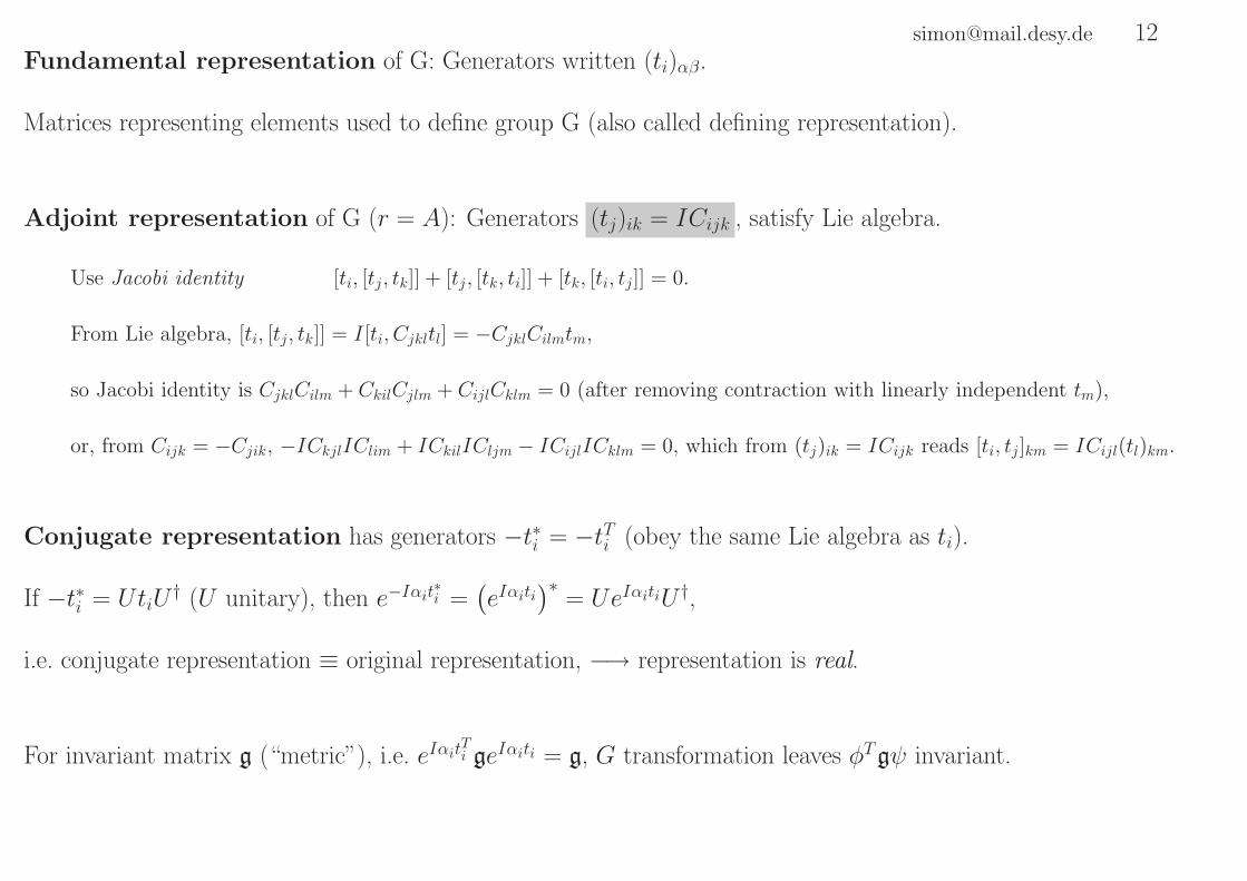
[email protected] 12Fundamental representation of G: Generators written (ti)αβ.
Matrices representing elements used to define group G (also called defining representation).
Adjoint representation of G (r = A): Generators (tj)ik = ICijk , satisfy Lie algebra.
Use Jacobi identity [ti, [tj, tk]] + [tj, [tk, ti]] + [tk, [ti, tj]] = 0.
From Lie algebra, [ti, [tj, tk]] = I[ti, Cjkltl] = −CjklCilmtm,
so Jacobi identity is CjklCilm + CkilCjlm + CijlCklm = 0 (after removing contraction with linearly independent tm),
or, from Cijk = −Cjik, −ICkjlIClim + ICkilICljm − ICijlICklm = 0, which from (tj)ik = ICijk reads [ti, tj]km = ICijl(tl)km.
Conjugate representation has generators −t∗i = −tTi (obey the same Lie algebra as ti).
If −t∗i = UtiU† (U unitary), then e−Iαit
∗i =
(eIαiti
)∗= UeIαitiU †,
i.e. conjugate representation ≡ original representation, −→ representation is real.
For invariant matrix g (“metric”), i.e. eIαitTi geIαiti = g, G transformation leaves φTgψ invariant.

[email protected] 13Semi-simple Lie algebra: no ti that commutes with all other generators (no U(1) subgroup).
Semi-simple group’s matrix generators must obey tr[ti] = 0.
Make all tr[ti] = 0 except one, tr[tK ], via t′i = Mijti (this is just rotation of vector with components tr[ti]).
Determinant of U(α)U(β) = U(γ) is eIαitr[ti]eIβitr[ti] = eIγitr[ti], i.e. (αi + βi − γi)tr[ti] = 0.
But only tr[tK ] 6= 0 (we assume), so αK + βK − γK = 0.
Must have CijKαiβj = 0 (recall γK ≃ αK + βK + CijKαiβj),
or CijK = CKij = 0 for all i, j, so from Lie group we have [tK , ti] = 0 for all i — not possible for semi-simple group.
So assumption was wrong, must have tr[tK ] = 0.

[email protected] 14Normalization of generators chosen as tr[titj] = C(r)δij .
Nij =tr[titj] becomes MikNkl(MT )lj after basis transformation ti →Mijtj.
Nij components of real symmetric matrix N , diagonalizable via MNMT when M real, orthogonal.
Also N is positive definite matrix αTNα = αitr[titj]αj =tr[αitiαjtj] =tr[(αiti)†αjtj] ≥ 0
(because for any matrix A, tr[A†A] = A†βαAαβ = A∗
αβAαβ =∑
αβ |Aαβ|2 ≥ 0).
After diagonalization, Nij = 0 for i 6= j and above implies Nii > 0 (no sum).
Then multiply each ti by real number ci, changes Nii → c2iNii > 0.
Choose ci such that each Nii (no sum over i) all equal to positive C(r).
Representation dependence of quadratic Casimir operator: C2(r)m(r) = C(r)d(G) .
Definition of quadratic Casimir operator gives tr[t2] = C2(r)m(r).
Normalization of generators tr[titj] = C(r)δij =⇒ tr[t2] = C(r)d(G).
Example: 2 and 3 component repesentations of rotation group have different spins (i.e. C2(r))12 and 1.

[email protected] 15Antisymmetric structure constants: Cijk = − I
C(r)tr[[ti, tj]tk] .
From Lie algebra, tr[[ti, tj]tl] = ICijktr[tktl] = ICijlC(r).
Structure constants obey CjkiClki = C(A)δjl .
In adjoint representation, quadratic Casimir operator on page 11 is (t2)jl = C2(A)δjl = −CjikCkil.
But C2(A) = C(A):
C2(A)m(A) = C(A)d(G) from representation dependence of quadratic Casimir operator on page 14,
and m(A) = d(G).

[email protected] 162.3 External symmetries
2.3.1 Rotation group representations
(Spatial) rotation of vector v → Rv preserves vTv, so R orthogonal (RTR = 1).
Rotation |θ| about θ: U(θ) = e−IJ ·θ .
Lie algebra is [Ji, Jj] = IǫijkJk for generators J1, J2, J3 (see later).
Or use J3 and raising/lowering operators J± = (J1 ± IJ2).

[email protected] 17Irreducible spin j representations:
(J(j)3 )m′m = mδm′m and (J
(j)± )m′m = [(j ∓m)(j ±m + 1)]δm′,m±1 , where m = −j,−j + 1, ..., j ,
spin j = 0, 12, 1, ... , number of components n.o.c.= 2j + 1 and J2 = j(j + 1) .
Let |m, j〉 be J3 = m and J2 = F (j) orthonormal eigenstates ([J3,J2] = 0).
J± changes m by ±1 because [J±, J3] = ∓J±, so J±|m, j〉 = C±(m, j)|m± 1, j〉.
C∓(m, j) =√F (j) −m2 ±m (states absorb complex phase):
|C∓(m, j)|2 = 〈m, j|J±J∓|m, j〉 (J †± = J∓) and J±J∓ = J2 − J2
3 ± J3.
Let j be largest m value for given F (j)
(m bounded because m2 = 〈m, j|J23 |m, j〉 = F (j) − 〈m, j|J2
1 + J22 |m, j〉 < F (j)).
F (j) = j(j + 1) because J+|j, j〉 = 0, so J−J+|j, j〉 = (F (j) − j2 − j)|j, j〉 = 0.
Let −j′ be smallest m: J−| − j′, j〉 = 0 =⇒ F (j) = j′(j′ + 1), so j′ = j (other possibility −j′ = j + 1 > j).
So m = −j,−j + 1, ..., j, i.e. n.o.c.= 2j + 1. Since n.o.c. is integer, j = 0, 12 , 1, ....

[email protected] 18Spin decomposition of tensors: e.g. 2nd rank tensor Cij (n.o.c.=9), representations are j = 0, 1, 2:
scalar (n.o.c.=1) + antisymmetric rank 2 tensor (n.o.c.=3) + symmetric traceless rank 2 (n.o.c.=5) components.
Cij = 13δijCkk + 1
2(Cij − Cji) + 12(Cij + Cji − 2
3δijCkk).
Component irreducible representations signified by 1 + 3 + 5.
Counting n.o.c. shows they are equivalent respectively to
the j = 0 (2j + 1 = 1), j = 1 (2j + 1 = 3) and j = 2 (2j + 1 = 5) representations:
13δijCkk → 1
3δijCkk is like scalar ≡ spin 0,
(12(Cjk − Ckj))|i6=k,j = 1
2ǫijkCjk → Ril12ǫljkCjk (because ǫR2 = Rǫ) is like vector ≡ spin 1,
12(Cij + Cji − 2
3δijCii) → RilRjm12(Clm + Cml − 2
3δlmCkk) is like rank 2 tensor ≡ spin 2.
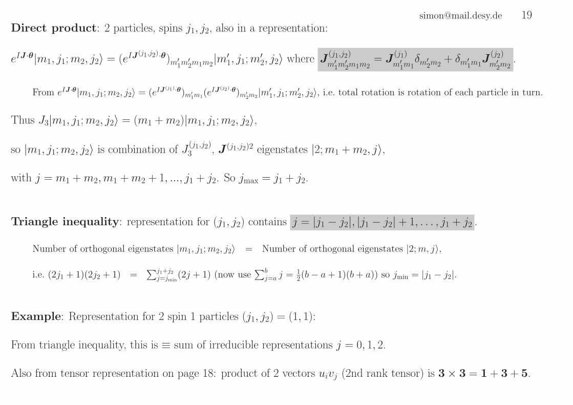
[email protected] 19Direct product: 2 particles, spins j1, j2, also in a representation:
eIJ ·θ|m1, j1;m2, j2〉 = (eIJ(j1,j2)·θ)m′
1m′2m1m2
|m′1, j1;m
′2, j2〉 where J
(j1,j2)
m′1m
′2m1m2
= J(j1)
m′1m1δm′
2m2+ δm′
1m1J
(j2)
m′2m2
.
From eIJ ·θ|m1, j1;m2, j2〉 = (eIJ(j1)·θ)m′
1m1(eIJ
(j2)·θ)m′2m2
|m′1, j1;m
′2, j2〉, i.e. total rotation is rotation of each particle in turn.
Thus J3|m1, j1;m2, j2〉 = (m1 +m2)|m1, j1;m2, j2〉,
so |m1, j1;m2, j2〉 is combination of J(j1,j2)3 , J (j1,j2)2 eigenstates |2;m1 +m2, j〉,
with j = m1 +m2,m1 +m2 + 1, ..., j1 + j2. So jmax = j1 + j2.
Triangle inequality: representation for (j1, j2) contains j = |j1 − j2|, |j1 − j2| + 1, . . . , j1 + j2 .
Number of orthogonal eigenstates |m1, j1;m2, j2〉 = Number of orthogonal eigenstates |2;m, j〉,
i.e. (2j1 + 1)(2j2 + 1) =∑j1+j2
j=jmin(2j + 1) (now use
∑bj=a j = 1
2(b− a+ 1)(b+ a)) so jmin = |j1 − j2|.
Example: Representation for 2 spin 1 particles (j1, j2) = (1, 1):
From triangle inequality, this is ≡ sum of irreducible representations j = 0, 1, 2.
Also from tensor representation on page 18: product of 2 vectors uivj (2nd rank tensor) is 3 × 3 = 1 + 3 + 5.

[email protected] 202.3.2 Poincare and Lorentz groups
Poincare (inhomogeneous Lorentz) group formed by coordinate transformations xµ → x′µ = Λµνx
ν + aµ,
preserving spacetime separation: gµνdxµdxν = gµνdx
′µdx′ν. Implies:
Transformation of metric tensor: gρσ = gµνΛµρΛ
νσ or (Λ−1)µν = Λ µ
ν .
Identity: Λµν = δµν, a
µ = 0 .
Poincare group defined by U(Λ, a)U(Λ, a) = U(ΛΛ,Λa + a) .
This is the double transformation x′′ = Λx′ + a = Λ(Λx+ a) + a.
Poincare group generators: Jµν and P µ , appearing in U(1 + ω, ǫ) ≃ 1 + 12IωµνJ
µν − IǫµPµ .
Obtained by going close to identity, Λµν = δµν + ωµν and aµ = ǫµ.
Choose Jµν = −Jνµ .
Allowed because ωρσ = −ωσρ: Transformation of metric tensor reads gρσ = gµν(δµρ + ωµρ)(δ
νσ + ωνσ) ≃ gσρ + ωρσ + ωσρ.

[email protected] 21Transformation properties of P µ, Jµν: U(Λ, a)P µU †(Λ, a) = Λ µ
ρ Pρ
and U(Λ, a)JµνU †(Λ, a) = Λ µρ Λ ν
σ (Jρσ − aρP σ + aσP ρ) .
Apply Poincare group to get U(Λ, a)U(1 + ω, ǫ)︸ ︷︷ ︸=U(Λ(1+ω),Λǫ+a)
U †(Λ, a)︸ ︷︷ ︸=U(Λ−1,−Λ−1a)
= U(1 + ΛωΛ−1,Λ(ǫ− ωΛ−1a)).
Expand both sides in ω, ǫ: U(Λ, a)(1 + 12IωJ − IǫP )U †(Λ, a) = 1 + 1
2IΛωΛ−1J − IΛ(ǫ− ωΛ−1a)P , equate coefficients of ω, ǫ.
So P µ transforms like 4-vector, Jij like angular momentum.
Poincare algebra: I [Jρσ, Jµν] = −gσνJρµ − gρµJσν + gσµJρν + gρνJσµ → (homogeneous) Lorentz group,
I [P µ, Jρσ] = gµρP σ − gµσP ρ , and [P µ, P ν] = 0 .
Obtained by taking Λµν = δµν + ωµν, aµ = ǫµ in transformation properties of P µ, Jµν, to first order in ω, ǫ gives
P µ − 12Iωρσ[P
µ, Jρσ] + Iǫν[Pµ, P ν] = P µ + 1
2ωρσgµσP ρ − 1
2ωρσgµρP σ, and
Jµν + 12Iωρσ[J
ρσ, Jµν] − Iǫρ[Pρ, Jµν] = Jµν − gρµǫρP
ν + gρνǫρPµ + 1
2ωρσ(gρνJσµ − gσνJρµ) + 1
2ωρσ(gσµJρν − gρµJσν).

[email protected] 222.3.3 Relativistic quantum mechanical particles
Identify H = P 0, spatial momentum P i, angular momentum Ji = 12ǫijkJ
jk (i.e. (J1, J2, J3) = (J23, J31, J12)).
[H,P ] = [H,J ] = 0 → P ,J conserved. Rotation group [Ji, Jj] = IǫijkJk is subgroup of Poincare group.
Also define boost generator K = (J10, J20, J30), obeys [Ji, Kj] = IǫijkKk and [Ki, Kj] = −IǫijkJk.
K not conserved: [Ki, H ] = IPi, because boost and time translation don’t commute.
Explicit form of Poincare elements:U(Λ, a) = e−IPµaµ︸ ︷︷ ︸
translate aµ
× e−IK·eβ︸ ︷︷ ︸boost along e by V=sinhβ
× eIJ ·θ︸︷︷︸rotate |θ| about θ
(V : magnitude of 4-velocity’s spatial part.)
Lorentz transformation of 4-vectors: (Ki)µν = I(δ0µδiν + δiµδ0ν) and (Ji)
µν = −Iǫ0iµν .
Then Aν → Aν − δωi(δiνA0 + δ0νAi) − δθiǫijνAj(1 − δ0ν) as required.
[e−IK·eβ]µ
ν=[1 − IKiei sinh β − (Kiei)
2 (cosh β − 1)]µν
and[eIJ ·θθ
]µν
=
[1 + IJiθi sin θ −
(Jiθi
)2
(1 − cos θ)
]µ
ν
.
Follows directly from (Kiei)3 = Kiei and (Jiθi)
3 = Jiθi.

[email protected] 23Particles: Use P µ, P 2 = m2 eigenstates. Distinguish momentum p from list σ, i.e. a†σ → a†σ(p).
Commutation relations for a(†)σ (p): [a†σ(p), a†σ′(p
′)]∓ = [aσ(p), aσ′(p′)]∓ = 0
and [aσ(p), a†σ′(p′)]∓ = δσσ′(2p
0)δ(3)(p − p′) .
As on page 4, but with different normalization (Lorentz invariant).
Application of general transformation of a(†)σ on page 10 to Lorentz transformation
complicated by mixing between σ and p.
Simplify by finding 2 transformations, one that mixes σ and one that mixes p, separately.
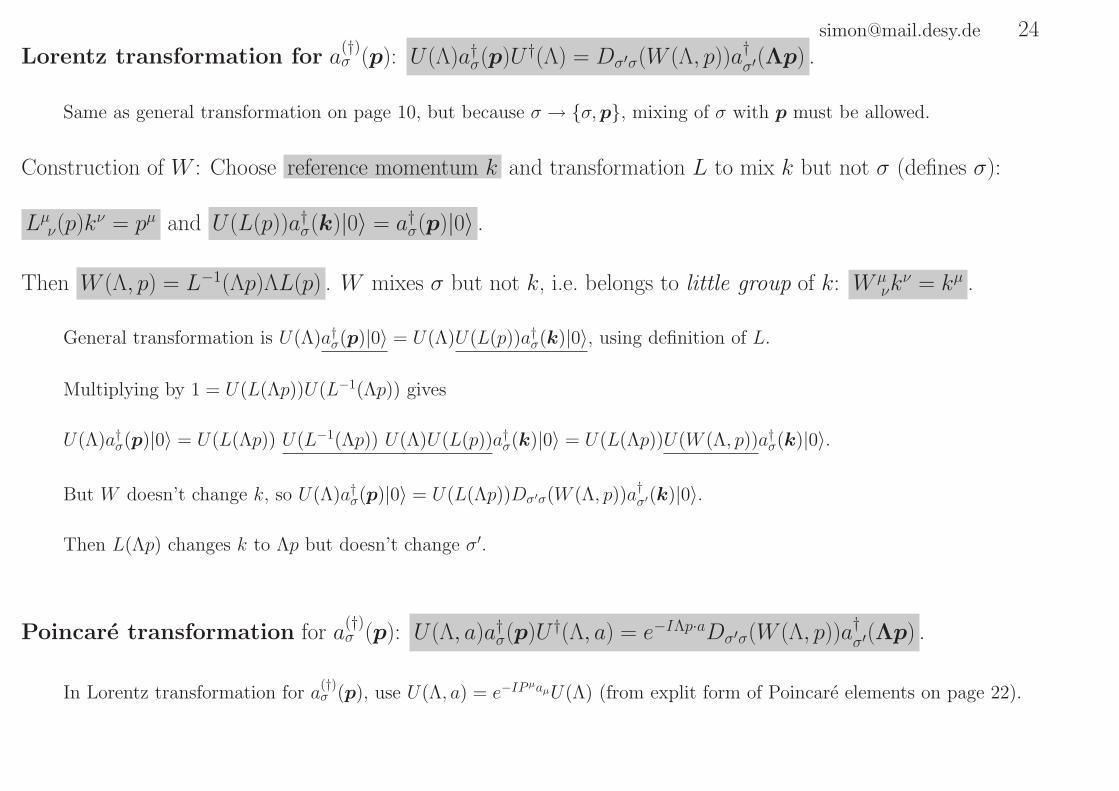
[email protected] 24Lorentz transformation for a
(†)σ (p): U(Λ)a†σ(p)U †(Λ) = Dσ′σ(W (Λ, p))a†σ′(Λp) .
Same as general transformation on page 10, but because σ → σ,p, mixing of σ with p must be allowed.
Construction of W : Choose reference momentum k and transformation L to mix k but not σ (defines σ):
Lµν(p)kν = pµ and U(L(p))a†σ(k)|0〉 = a†σ(p)|0〉 .
Then W (Λ, p) = L−1(Λp)ΛL(p) . W mixes σ but not k, i.e. belongs to little group of k: W µνk
ν = kµ .
General transformation is U(Λ)a†σ(p)|0〉 = U(Λ)U(L(p))a†σ(k)|0〉, using definition of L.
Multiplying by 1 = U(L(Λp))U(L−1(Λp)) gives
U(Λ)a†σ(p)|0〉 = U(L(Λp)) U(L−1(Λp)) U(Λ)U(L(p))a†σ(k)|0〉 = U(L(Λp))U(W (Λ, p))a†σ(k)|0〉.
But W doesn’t change k, so U(Λ)a†σ(p)|0〉 = U(L(Λp))Dσ′σ(W (Λ, p))a†σ′(k)|0〉.
Then L(Λp) changes k to Λp but doesn’t change σ′.
Poincare transformation for a(†)σ (p): U(Λ, a)a†σ(p)U †(Λ, a) = e−IΛp·aDσ′σ(W (Λ, p))a†σ′(Λp) .
In Lorentz transformation for a(†)σ (p), use U(Λ, a) = e−IP
µaµU(Λ) (from explit form of Poincare elements on page 22).
[email protected] 252.3.4 Quantum field theory
Lorentz invariant QM: H =∫d3xH (x) , scalar field H (x) (i.e. U(Λ, a)H (x)U †(Λ, a) = H (Λx + a) ),
obeys cluster decomposition principle (two processes with large spatial separation evolve independently).
Causality: [H (x),H (y)] = 0 when (x− y)2 ≥ 0 . Required for Lorentz invariance of S-matrix.
Intuitive reason: signal can’t propagate between 2 spacelike separated events.
In QM (general): H built from a(†)σ . In QFT: H built from H (x) built from products of
Fields ψ−cl (x) =
∫D3p vlσ(x; p)ac†σ (p) and ψ+
l (x) =∫D3p ulσ(x; p)aσ(p) .
Lorentz invariant momentum space volume D3p = d3p2p0 = d4pδ(p2 +m2)θ(p0) obeys D3Λp = D3p.
These fields should obey
Poincare transformation for fields: U(Λ, a)ψ(c)±l (x)U †(Λ, a) = Dll′(Λ
−1)ψ(c)±l′ (Λx + a) .
To calculate ulσ(x; p) and vlσ(x; p), take single particle species in representation labelled j, allow ac†σ (p) 6= a†σ(p).

[email protected] 26x dependence of u, v: ul σ(x; p) = eIp·xul σ(p) , vl σ(x; p) = e−Ip·xvl σ(p) .
Take Λ = 1 in Poincare transformation for fields and for a(†)σ (p) on page 25 and 24,
e.g. U(1, a)ψ+l (x)U †(1, a) =
∫D3p ulσ(x; p)U(1, a)aσ(p)U †(1, a) =
∫D3p eIp·aulσ(x; p)aσ(p)
= ψ+l (x+ a) =
∫D3p ulσ(x+ a; p)aσ(p), equate coefficients of aσ(p) (underlined), gives ul σ(x; p)eIp·a = ulσ(x+ a; p).
Klein-Gordon equation: (∂2 −m2)ψ±(c)l (x) = 0 .
Act on e.g. ψ−cl (x) =
∫D3p e−Ip·xvl σ(p)ac†σ (p) with (∂2 −m2), use p2 = −m2.
Transformation of u, v: Dll′(Λ)ul′σ(p) = D(j)σ′σ(W (Λ, p))ulσ′(Λp) , Dll′(Λ)vl′σ(p) = D
(j)σσ′(W
−1(Λ, p))vlσ′(Λp) .
E.g. consider v, use Poincare transformation for fields and for a(†)σ (p) on page 25 and 24.
LHS: U(Λ, a)ψ−cl (x)U †(Λ, a) =
∫D3p vlσ(x; p)U(Λ, a)ac†σ (p)U †(Λ, a) =
∫D3p e−IΛp·avlσ(x; p)D
(j)σ′σ(W (Λ, p))ac†σ′(Λp), and
RHS: Dll′(Λ−1)ψ−c
l′ (Λx+ a) =∫D3p Dll′(Λ
−1)vlσ(Λx+ a; p)ac†σ (p) =∫D3Λp Dll′(Λ
−1)vlσ(Λx+ a;Λp)ac†σ (Λp) (p→ Λp).
Use D3Λp = D3p, equate coefficient of ac†σ (Λp) (underlined), multiply by Dl′′l(Λ)D(j)σ′′σ(W
−1(Λ, p)).
p dependence of u, v: ulσ(p) = Dll′(L(p))ul′σ(k) . (p dependence of v is the same.)
In transformation of u, v, take p = k so L(p) = 1, Λ = L(q) so Λp = L(q)k = q, then W (Λ, p) = L−1(Λp)L(q) = 1.

[email protected] 272.3.5 Causal field theory
Since [ψ+l (x), ψ−c
l′ (x′)]∓ 6= 0, causality on page 25 only gauranteed by taking H (x) to be functional of
complete field ψl(x) = κψ+l (x) + λψ−c
l (x) (so representations Dll′(Λ−1) for ψ+
l (x) and ψ−cl (x) the same), with
Causality: [ψl(x), ψl′(y)]∓ = [ψl(x), ψ†l′(y)]∓ = 0 when (x− y)2 > 0 by suitable choice of κ, λ.
Now 〈0|H|0〉 = ∞, i.e. consistency with gravity not gauranteed by QFT.
In each term in H, last operator on right hand side is not always an annihilation operator.
Complete field: ψl(x) =∫D3p
[κeIp·xulσ(p)aσ(p) + λe−Ip·xvlσ(p)ac†σ (p)
].

[email protected] 282.3.6 Antiparticles
H (x) commutes with conserved additive Q: [Q,H (x)] = 0 .
Imposed in order to satisfy [Q,H] = 0.
This is achieved as follows:
Commutation of fields with conserved additive Q: [Q,ψl(x)] = −qlψl(x) , and
Field construction of H (x): H =∑ψL1l1ψL2l2. . . ψM1†
m1ψM2†m2
. . . with qL1l1
+ qL2l2
+ . . .− qM1m1
− qM2m2
− . . . = 0
(Mi, Lj label particle species).
Antiparticles: For every particle species there is another species with opposite conserved quantum numbers .
Commutation of fields with conserved additive Q implies [Q,ψ−cl (x)] = −qlψ−c
l (x) and [Q,ψ+l (x)] = −qlψ+
l (x),
but since [Q, ac†σ ] = qcσac†σ and [Q, aσ] = −qσaσ (no sum) from page 5, ql = qcσ and ql = −qσ, i.e. qcσ = −qσ.
[email protected] 292.3.7 Spin in relativistic quantum mechanics
Lorentz group algebra simplified by choosing generators Ai = 12(Ji − IKi) and Bi = 1
2(Ji + IKi) ,
behaves like 2 independent rotations: [Ai, Aj] = IǫijkAk , [Bi, Bj] = IǫijkBk and [Ai, Bj] = 0 ,
i.e. relativistic particle of type (A,B) (i.e. in eigenstate of A2 = A(A + 1), B2 = B(B + 1))
≡ 2 particles at rest, ordinary spins A, B (in representation sense).
In terms of degrees of freedom, (A,B) = (2A+1) × (2B+1).
Triangle inequality: ordinary spin J = A + B , so j = |A−B|, |A−B| + 1, ..., A +B .
Derived on page 19.
Can have eigenstates of A2 = A(A + 1), B2 = B(B + 1) and J2 = j(j + 1) simultaneously,
because [J2, Ai] = [J2, Bi] = 0 . Use J2 = (A + B)2 and A, B commutation relations.
Simultaneous eigenstate also with any K = I(A − B) or K2 not possible.

[email protected] 30Example: (A,B) = (1
2,12) is representation of 4-vector: (A3)
µν, (B3)
µν can have eigenvalues ±1
2 only.
From triangle inequality on page 29, j = 0, 1.
Also follows from tensor representation on page 18: 2 × 2 = 1 + 3.
More generally, rank N tensor is (12,
12)N =
∑N2A=0
∑N2B=0(A,B),
i.e. (12,
12)N =
(N2 ,
N2
)+lower spins, where
(N2 ,
N2
)≡ traceless symmetric rank N tensor, j = 0, ..., N .
(N, 0) and (0, N) are purely spin j = N .

[email protected] 312.3.8 Irreducible representation for fields
If particles created by a(c)†σ (p) have spin j (i.e. [J2, a
(c)†σ (p)] = j(j + 1)a
(c)†σ (p)),
must take field with same spin j but any (A,B) consistent with triangle inequality on page 29:
ψab(x) =∫D3p
[κ eIp·xuab σ(p)aσ(p) + λ e−Ip·xvab σ(p)ac†σ (p)
](l = ab, l′ = a′b′),
Lorentz transformation uses generators Aa′b′ab = J(A)a′a δb′b , Ba′b′ab = δa′aJ
(B)b′b
where a = −A,−A + 1, ..., A and b = −B,−B + 1, ..., B .

[email protected] 322.3.9 Massive particles
Choose k = (0, 0, 0,m) (momentum of particle at rest) Then W is an element of the spatial rotation group.
L(p) in terms of K: L(p) = exp[−Ip · Kβ] .
Then W (R, p) = R, i.e. rotation group apparatus of subsubsection 2.3.1 applies to relativistic particles too.
Conditions on u, v: J(j)σ′σuab σ′(0) = J
(A)aa′ ua′b σ(0) + J
(B)bb′ uab′ σ(0) , −J
(j)∗σ′σ vab σ′(0) = J
(A)aa′ va′b σ(0) + J
(B)bb′ vab′ σ(0) .
In transformation of u, v on page 26, take Λ = R and p = 0 (i.e. p = k)
(so p = k, Rp = p, L(p) = 1, W (R, p) = L−1(Rp)RL(p) = L−1(p)R = R), so e.g. Dll′(R)vl′σ(0) = D(j)σσ′(R−1)vlσ′(0),
and use D(j)σσ′(R−1) = D
(j)∗σ′σ (R) because irreducible representations of R are unitary (see form of (J
(j)i )σ′σ on page 17).
Take l = ab, so Daba′b′(R)va′b′σ(0) = D(j)∗σ′σ (R)vabσ′(0). Generators of D(j)∗(R), D(R) are respectively −J (j)∗, A + B.
u, v relation: vab σ(0) = (−1)j+σuab −σ(0) up to normalization.
Conditions on u, v with (no sum over σ, σ′) −J(j)∗σσ′ = (−1)σ−σ
′
J(j)−σ,−σ′ from page 17
gives vab σ(0) ∝ (−1)σuab −σ(0), absorb proportionality constant into u, v.
The p dependence of u, v are the same, so vab σ(p) = (−1)j+σuab −σ(p) .

[email protected] 332.3.10 Massless particles
Take reference vector k = (0, 0, 1, 1).
Little group transformation: W (θ, µ, ν) ≃ 1 + IθJ3 + IµM + IνN with M = J2 +K1, N = −J1 +K2 .
W has 3 degrees of freedom: For (ti)µνk
ν = 0, take ti = (J3,M,N), check with Lorentz transformation of 4-vectors on page 22.
Choice of states: (J3,M,N)|k, σ〉 = (σ, 0, 0)|k, σ〉 .
Since [M,N ] = 0, try eigenstates for which M |k,m, n〉 = m|k,m, n〉, N |k,m, n〉 = n|k,m, n〉.
Then m, n continuous degrees of freedom, unobserved: [J3,M ] = IN , so M(1 − IθJ3)|k,m, n〉 = (m− nθ)(1 − IθJ3)|k,m, n〉,
i.e. (1 − IθJ3)|k,m, n〉 is eigenvector of M , eigenvalue m− nθ.
Similarly, [J3, N ] = −IM , so (1 − IθJ3)|k,m, n〉 is eigenvector of N , eigenvalue n+mθ.
Avoid this problem by taking m = n = 0, so left with states J3|k, σ〉 = σ|k, σ〉.
Since J3 = J · k, σ is helicity, component of spin in direction of motion.
Representation for massless particles: Dσ′σ(W ) = eIθσδσ′σ .
U(W )|k, σ〉 = (1 + IθJ3 + IµM + IνN)|k, σ〉 = (1 + Iθσ)|k, σ〉. For finite θ, U(W )|k, σ〉 = eIθσ|k, σ〉.
[email protected] 34p dependence of u: ul σ(p) = Dll′(L(p))ul′ σ(k) . (p dependence of v is the same.) As on page 26.
Little group transformation of u, v: ul σ(k)eIθ(W,k)σ = Dll′(W )ul′ σ(k) , vl σ(k)e−Iθ(W,k)σ = Dll′(W )vl′ σ(k) .
Transformation of u, v on page 26 reads ul σ(Λp)eIθ(Λ,p)σ = Dll′(Λ)ul′ σ(p). Take Λ = W , p = k.
Rotation of u, v: (J3)ll′ul′ σ(k) = σul σ(k) , (J3)ll′vl′ σ(k) = −σvl σ(k) .
Take W to be just rotation about 3-axis (W (θ, µ, ν) ≃ 1 + IθJ3, i.e. µ = ν = 0) in little group transformation of u, v.
M , N transformation of u, v: Mll′ul′ σ(k) = Nll′ul′ σ(k) = 0 . Same for v.
Take W = (1 + IµM + IνN) in little group transformation of u, v.
u, v relation: vl σ(p) = u∗l σ(p) .
Implied (up to proportionality constant) by rotation (note (J3)ll′ is imaginary) and M , N transformation of u, v.
Allowed helicities for fields in given (A,B) representation: σ = ±(B − A) for particle/antiparticle .
J = A + B, and e.g. A3aba′b′ = aδaa′δbb′, so rotation of u is σuab σ(k) = (a+ b)uab σ(k).
M , N transformation of u is Maba′b′ua′b′ σ = Naba′b′ua′b′ σ = 0. Using M = IA− − IB+ and N = −A− −B+,
where A± = A1 ± IA2, B± = B1 ± IB2 are usual raising/lowering operators, (A−)aba′b′ua′b′ σ = (B+)aba′b′ua′b′ σ = 0,
i.e. must have a = −A, b = B or uab σ = 0. So σ = B − A. Similar for v, gives σ = A−B.

[email protected] 352.3.11 Spin-statistics connection
Determine which of ∓ for given j is possible for causality on page 27 to hold. Demand more general condition
[ψab(x), ψ†ab
(y)]∓ =∫D3p πab,ab(p)
[κκ∗eIp·(x−y) ∓ λλ∗e−Ip·(x−y)
]= 0 for (x− y)2 > 0,
where ψab, ψab for same particle species and πab,ab(p) = uab σ(p)u∗ab σ
(p) = vab σ(p)v∗ab σ
(p).
In field on page 31, use commutation relations for a(†)σ (p) on page 23.
uab σ(p)u∗ab σ
(p) = vab σ(p)v∗ab σ
(p) holds for massive particles from u, v relation on page 32.
(uab σ(p)u∗ab σ
(p) = [vab σ(p)v∗ab σ
(p)]∗ in massless case from u, v relation on page 34).
Relation between κ, λ of different massive fields: κκ∗ = ±(−1)2A+2Bλλ∗ .
Explicit calculation shows πab,ab(p) = Pab,ab(p) + 2√
p2 +m2Qab,ab(p),
where (P,Q)(p) are polynomial in p, obey (P,Q)(−p) = (−1)2A+2B(P,−Q)(p).
Take (x− y)2 > 0, use frame x0 = y0, write ∆+(x) =∫D3peIp·x:
[ψab, ψab]∓ =[κκ∗ ∓ (−1)2A+2Bλλ∗
]Pab,ab(−I∇)∆+(x − y, 0) +
[κκ∗ ± (−1)2A+2Bλλ∗
]Qab,ab(−I∇)δ(3)(x − y).
Commutator must vanish for x 6= y, so coefficient of P zero.

[email protected] 36Relations between κ, λ of single field: |κ|2 = |λ|2 and ±(−1)2A+2B = 1 .
For A = A, B = B, relation between κ, λ of different fields reads |κ|2 = ±(−1)2A+2B|λ|2.
Spin-statistics: Bosons (fermions) have even (odd) 2j and vice versa .
From triangle inequality on page 29,
j − (A+B) is integer, so ±(−1)2j = 1, i.e. in [ψab, ψab]∓, must have − (+) for even (odd) 2j.
Relation between κ, λ of single massive field: λ = (−1)2AeIcκ , c is the same for all fields.
Divide relation between κ, λ of different massive fields on page 35 by |κ|2 = |λ|2: κκ = ±(−1)2A+2B λ
λ= (−1)2A+2A λ
λ.
Absorb κ into field, eIc into ac†σ (p) (does not affect commutation relations on page 23).
(−1)2A can’t be absorbed into ac†σ (p) since this is independent of A,
nor absorbed into v since this is already chosen. So
Massive irreducible field: ψab(x) =∫D3p
[eIp·xuab σ(p)aσ(p) + (−1)2Ae−Ip·xvab σ(p)ac†σ (p)
],
or more fully as ψab(x) =∫D3p D
(j)aba′b′(L(p))
[eIp·xua′b′ σ(0)aσ(p) + (−1)2A+j+σe−Ip·xua′b′ −σ(0)ac†σ (p)
].
Use u, v relation on page 32.

[email protected] 372.4 External symmetries: fermions
2.4.1 Spin 12 fields
2j is odd −→ particles are fermions. j = 12 representations include (A,B) =
(12, 0)
and (A,B) =(0, 1
2
).
In each case, group element acts on 2 component spinor X(A,B) (X(A,B) is e.g. a field operator),
with 2 components X(A,B)ab :
X(12 ,0) ≡ XL =
(X
(12 ,0)
12 ,0
, X(1
2 ,0)−1
2 ,0
)(“left-handed”) and
X(0,12) ≡ XR =
(X
(0,12)0,12
, X(0,12)0,−1
2
)(“right-handed”).
“Handedness”/chirality refers to eigenstates of helicity for massless particles (see later).

[email protected] 38Lorentz transformation of spinors: U(Λ)XL/RU
†(Λ) = hL/R(Λ)XL/R (D acts on the 2 a, b components).
From explicit form of Lorentz group elements on page 22, hL/R(Λ) = eIJ(1
2 ,0)/(0,12)·θe−IK(1
2 ,0)/(0,12)·eβ, where
Lorentz group generators for spinors: J(1
2 ,0)i = 1
2σi, K(1
2 ,0)i = I 1
2σi , J(0,12)i = 1
2σi, K(0,12)i = −I 1
2σi ,
where σi are the Pauli σ matrices σ1 =
(0 1
1 0
), σ2 =
(0 −II 0
)and σ3 =
(1 0
0 −1
), which obey
Rotation group algebra:[
12σi,
12σj]
= Iǫijk12σk .
Follows from Ji = J(A)i + J
(B)i and Ki = I(J
(A)i − J
(B)i ) on page 29,
and J(0)i = 0 and J
(12)
i = 12σi from irreducible representation for spin j on page 17.
Explicit form of hL/R: hL/R = eI12σiθie∓
12σieiβ . Note σ matrices are Hermitian.
Product of σmatrices: σiσj = δij + Iǫijkσk . Follows by explicit calculation.
Direct calculation of hL/R: hL/R = (cos θ2 + Iσiθi sinθ2)(cosh β
2 ∓ σiei sinh β2 ) .
From product of σ matrices, T 2 = 1 where T = σiei (T = σiθi). Then exT = coshx+ T sinhx (eIxT = cosx+ IT sinx).

[email protected] 39Write hL = h and XL = X which has components Xa = (X1, X2) , which transforms as 1. X ′
a = h ba Xb .
Can also define spinor transforming with h∗: Use dotted indices for h∗, so 2. X ′†a = h∗ b
a X†b
.
Then hR = h∗−1T . From explicit form of hL/R on page 38.
Use upper indices for h−1, andXR has components X†a = (X†1, X†2) , Dotted indices because h∗ is used.
transformation is 4. X ′†a =(h∗−1T
)abX†b , where we define (hT )a b = h a
b .
Conjugate of this turns dotted indices into undotted indices, so 3. X ′a =(h−1T
)abXb .
Conjugate of spinors: (Xa)† = X†a , (Xa)† = X†
a . Definition of X†a in terms of Xa, X†a in terms of Xa.
Check that if Xa transforms as transformation 1., X†a transforms as transformation 2.: X ′†
a = (X ′a)
† = (h ba Xb)
† = h∗ba X†b.

Spinor metric: ǫab =
(0 1
−1 0
), ǫab = −ǫab. Note ǫabǫ
bc = δ ca . ǫ is unitary matrix.
Pseudo reality: ǫac(σi)dc ǫdb = −(σTi )ab .
Follows by explicit calculation. Since σ∗i = σTi , shows rotation group representation by σ matrices is real (see page 12).
X†a is
(0, 1
2
), i.e. right-handed, like X†a.
Pseudo reality above implies ǫach∗dc ǫdb = (h∗−1T )ab, i.e. h∗, hR same up to unitary similarity transformation.
For unitary representations, follows because A = B† from definition on page 29, so conjugation makes(
12 , 0)→(0, 1
2
).
This means dotted indices are for right-handed ((0, 1
2
)) fields.
(Similarly, undotted indices are for left-handed ((
12, 0)) fields.)
Metric condition: h∗ de ǫdb(h
∗T )bf
= ǫef .
Follows from ǫach∗dc ǫdb = (h∗−1T )ab
result above. Thus ǫ is the group’s invariant matrix g (“metric”) on page 12.

[email protected] 41Raising and lowering of spinor indices: Xa = ǫabXb . This is definition of Xa in terms of Xa.
Follows that Xa = ǫabXb . Same definition / behaviour for dotted indices.
Check that if Xa transforms as transformation 1. on page 39, Xa transforms as transformation 3.: X ′a = ǫabX ′b = ǫabh c
b Xc.
From pseudo reality, ǫabh cb ǫcd =
(h−1T
)ad, or ǫabh c
b =(h−1T
)abǫbc, so X ′a =
(h−1T
)abǫbcXc =
(h−1T
)abXb.
Right-handed from left-handed fields: X†a =(ǫabXb
)†.
So all fields can be expressed in terms of left-handed fields.
Scalar from 2 spinors: XY = XaYa = −YaXa = Y aXa = −XaYa = Y X .
Xa′Y ′a =
(h−1T
)acXch b
a Yb =(h−1) a
ch ba X
cYb. X, Y anticommute (spinor operators). XaYa = −XaYa because ǫabǫac = −δbc.
Hermitian conjugate of scalar: (XY )† = (XaYa)† = (Ya)
†(Xa)† = Y †aX
†a = Y †X† .

4-vector σ matrices σµab
: σiab
= (σi)ab, σ0ab
= (σ0)ab and σ0 =
(1 0
0 1
).
4-vector σ matrices with raised indices: σµ ab = ǫbcσµcdǫad , so σi ab = −(σi)
ab, σ0 ab = (σ0)ab .
Second result follows from definition by explicit calculation.
Inner product of 4-vector σ matrices: gρωσωefσρ ba = −2δ a
e δbf
.
Outer product of 4-vector σ matrices: σνabσρ ba = −2gνρ .
XaσµabY †b is a 4-vector .
Need to show X ′aσµabY ′†b = Λµ
νXaσν
abY †b. Since X ′aσµ
abY ′†b =
(h−1T
)acXcσµ
ab
(h∗−1T
)bdY †d,
need to show(h−1) c
aσµcd
(h∗−1T
)db= Λµ
νσνab
. Contracting with σρ ba and using outer product of 4-vector σ matrices
gives Λµρ = −12σ
ρ ba(h−1) c
aσµcd
(h∗−1T
)db= −1
2tr[σρh−1σµh∗−1T
], which is equivalent because σ matrices linearly independent
(or multiply this by gρωσωef
and use inner product of 4-vector σ matrices). Check group property:
ΛµνΛ
′νρ = 1
2tr[σµh−1(Λ)σνh∗−1T (Λ)
]12tr[σνh−1(Λ′)σρh∗−1T (Λ′)
]= 1
2σµijhjk(Λ)σµklh
†li(Λ)σνmnhnp(Λ
′)σρpqh†qm(Λ′). From
inner product of 4-vector σ matrices, σνmnσµkl = −2δmlδkn, so ΛµνΛ
′νρ = −1
2σµ ba
(h−1(Λ′)h−1(Λ)
) c
aσρcd
(h∗−1T (Λ)h∗−1T (Λ′)
)db

[email protected] 43Convenient to put left- (X) and right-handed (Z) fields together as 4 component spinor:
ψT =
(C1X
(12 ,0)
12 ,0
, C1X(1
2 ,0)−1
2 ,0, C2Z
(0,12)0,12
, C2Z(0,12)0,−1
2
), where C1, C2 scalar constants.
Lorentz group generators: Ji =
(12σi 0
0 12σi
)and Ki =
(I 1
2σi 0
0 −I 12σi
).
Follows from Lorentz group generators for spinors on page 38.
This is the chiral (Weyl) representation,
others representations from similarity transformation: J ′i = V JiV
−1, K ′i = V KiV
−1, X ′ = V X etc.
Preferable to express in terms of left-handed fields only:
ψ =
(Xa
(ǫbcYc)†
)=
(Xa
Y †b
), where Y = Z† is left-handed like X .

[email protected] 442.4.2 Spin 1
2 in general representations
Any 4×4 matrix can be constructed from sums/products of gamma matrices (next page):
Gamma matrices (chiral representation): γ0 = −I(
0 1
1 0
)and γi = −I
(0 σi
−σi 0
), or γµ = −I
(0 σµ
σµ 0
).
Gamma matrix in different representations related by similarity transformation γ′µ = V γµV −1 .
Anticommutation relations for γµ: γµ, γν = 2gµν . This is representation independent.
Check by explicit calculation in chiral representation, use rotation group algebra on page 38.
Define γ5 =
(1 0
0 −1
)= −Iγ0γ1γ2γ3. Check last representation-independent equality explicitly in chiral representation.
Then PL = 12(1 + γ5) =
(1 0
0 0
)projects out left-handed spinor: PL
(Xa
(ǫbcYc)†
)=
(Xa
0
),
similarly PR = 12(1 − γ5) =
(0 0
0 1
)projects out right-handed spinor: PR
(Xa
(ǫbcYc)†
)=
(0
(ǫbcYc)†
).
Note PL/R are projection operators: P 2L/R = PL/R, PL/RPR/L = 0.
[email protected] 45Any 4×4 matrix is linear combination of 1, γµ, [γµ, γν], γµγ5, γ5.
Because these are 16 non-zero linearly independent 4×4 matrices.
Non-zero because their squares, calculated from anticommutation relations on page 44, are non-zero.
Linearly independent because they are orthogonal if we define scalar product of any two to be trace of their matrix product:
tr[1γµ] = 0, because tr[γµ] = 0 in chiral representation, therefore in any other representation.
tr[1[γµ, γν]] = 0 by (anti)symmetry. From anticommutation relations, tr[1γµγ5] = −tr[γ5γµ] = −tr[γµγ5] = 0
and also tr[1γ5] =tr[γ5] = 0 by commuting γ0 from left to right.
Next, tr[γρ[γµ, γν]] = 0: From anticommutation relations, γ25 = −γ0γ1γ2γ3γ0γ1γ2γ3 = −γ0 2γ1 2γ2 2γ3 2 = 1.
So tr[γρ[γµ, γν]] =tr[γ25γ
ρ[γµ, γν]] = − tr[γ5γρ[γµ, γν]γ5] =tr[γ5γ
ρ[γµ, γν]γ5].
To show tr[γργµγ5] = 0, first consider case ρ = µ. Then γργµ = gρρ, and result is ∝tr[γ5] = 0.
If e.g. ρ = 1, µ = 2, tr[γργµγ5] = Itr[γ0γ3] = 0. tr[γµγ5] = 0 already shown.
tr[[γµ, γν]γργ5] = 0 from anticommutation relations. tr[[γµ, γν]γ5] = 0 because tr[γργµγ5] = 0. Finally tr[γµγ5γ5] =tr[γµ] = 0.
So all spinorial observables expressible as representation independent sums/products of gamma matrices.

[email protected] 46Lorentz group generators from γµ: Jµν = −I
4 [γµ, γν] .
Explicit calculation in chiral representation, Ji = 12ǫijkJjk, K = (J10, J20, J30),
Lorentz group generators on page 43, Gamma matrices on page 44.
Similarity transformation on page 43 equivalent to similarity transformation on page 44.
Infinitesimal Lorentz transformation of γµ: I [Jµν, γρ] = gνργµ − gµργν ,
Follows from anticommutation relations for γµ on page 44 and Lorentz group generators from γµ above.
Lorentz transformation of γµ: D(Λ)γµD−1(Λ) = Λ µν γ
ν , i.e. γµ transforms like a vector.
Agrees with infinitesimal Lorentz transformation of γµ, because for infinitesimal case,
LHS is (1 + 12IωρσJ
ρσ)γµ(1 − 12IωωηJ
ωη) = γµ − 12Iωρσ[γ
µ, Jρσ], and RHS is (δ µν + ωνσg
µσ)γν = γµ − 12ωρσ(g
µργσ − gµσγρ).
Lorentz transformation of vector: γµ(Λp)µ = D(Λ) γµpµ D−1(Λ) .
From Lorentz transformation of γµ above.
Reference boost:γµpµm = −D(L(p))γ0D−1(L(p)) . Equivalent of p = L(p)k on page 24, −γ0m = γµkµ.
In Lorentz transformation of vector, take p = k, Λ = L(q). Then γµqµ = D(L(q)) γµkµ D−1(L(q)) = −D(L(q)) γ0m D−1(L(q)).

Parity transformation matrix: β = Iγ0 =
(0 1
1 0
). Note β2 = 1.
Pseudo-unitarity of Lorentz transformation : Jµν† = βJµνβ , D† = βD−1β .
βγ0β = γ0 = −γ0† and βγiβ = −γi = −γi†, or βγµβ = −㵆. Then use Lorentz group generators from γµ on page 46.
Infinitesimal D† is 1 − 12IωmuνJ
µν† = β(1 − 12IωmuνJ
µν)β.
Adjoint spinor: X = X†β . Allows construction of scalars, vectors etc. from spinors:
Covariant products: XY is scalar , XγµY is vector .
First case: X ′Y ′ = X ′†βY ′ = X†D†βDY .
From pseudo-unitarity of Lorentz transformation, D†β = βD−1β2 = βD−1, so X ′Y ′ = X†βD−1DY = X†βY = XY .
Second case: X ′γµY ′ = X†D†βγµDY = X†βD−1γµDY . Lorentz transformation of γµ on page 46 can be rewritten
D−1γµD =(Λ−1
) µ
νγν = Λµ
νγν, so X ′γµY ′ = Λµ
νX†βγνY = Λµ
νXβγνY .
Vanishing products: ψR/LψL/R and ψL/RγµψL/R , where ψL/R = PL/Rψ (see page 44 for PL/R).
Using γ†5 = γ5 in chiral representation and PL/Rβ = βPR/L gives ψRψL = ψ†PLβPLψ = ψ†βPRPLψ = 0 (because PL/RPR/L = 0).
Similarly, using γµγ5 = −γ5γµ, one has ψLγ
µψL = ψ†PRβγµPLψ = ψ†βγµPRPLψ = 0.

[email protected] 48Problems 1
1: If the parameterization αi of group elements U(α), chosen such that U(0) = 1, can be chosen such that the Abelianlimit U(α)U(β) = U(α + β) is obeyed for βi = cαi, show that U(α) = exp [Itiαi]. Hint: Use the Abelian limit to write
U(α) =[U(
αN
)]N, take N → ∞, expand U
(αN
)= 1 + Iti
αiN + O
(1N2
)and use ex =
∑∞k=0
xk
k! and the binomial theorem
(x+ y)N =∑N
k=0N !
k!(N−k)!xkyN−k.
2: Show that the symmetry transformation U(α)a†σa†σ′ . . . |0〉 = Dσσ′′(α)Dσ′σ′′′(α)a†σ′′a
†σ′′′ . . . |0〉 and U(α)|0〉 = |0〉 is uniquely
satisfied by the condition U(α)a†σU†(α) = Dσσ′(α)a†σ′. Show that the matrices D furnish a representation of the group
defined by U (namely γ(α,β) in U(γ(α,β)) = U(α)U(β)).
3: Show that a semi-simple group’s matrix generators ti all obey tr[ti] = 0.
4: Use the Lorentz group algebra I[Jρσ, Jµν] = −gσνJρµ − gρµJσν + gσµJρν + gρνJσµ to derive the rotation group algebra[Ji, Jj] = IǫijkJk, where (J1, J2, J3) = (J23, J31, J12).
5: Using the explicit result for the generator of 4-vector boosts, namely (Ki)µν = I(δ0µδiν+δiµδ0ν), show that the explicit cal-
culation of a general boost is[e−IK·eβ]µ
ν=[1 − IKiei sinh β − (Kiei)
2 (cosh β − 1)]µν. Hint: Show by explicit calculation
the result (Kiei)3 = Kiei and then use it.
6: Define a field ψc−l (x) =∫D3p vlσ(x; p)ac†σ (p), where vlσ(x; p) is such that ψc−l (x) has the transformation property
U(Λ, a)ψc−l (x)U †(Λ, a) = Dll′(Λ−1)ψc−l′ (Λx + a). Show that Dll′(Λ)vl′σ(p) = D
(j)σσ′(W−1(Λ, p))vlσ′(Λp), where vlσ(p) =
vlσ(0; p). For a massive particle, for reference momentum k = (0, 0, 0, 1) and for L a pure boost, show that this implies
that −J(j)∗σ′σ vab σ′(0) = J
(A)aa′ va′b σ(0) + J
(B)bb′ vab′ σ(0). Hint: Take Λ = R and p = k.
7: Show that J(1
2 ,0)i = 1
2σi and K( 1
2 ,0)i = I 1
2σi. Hint: Use J = A+B and K = I(A−B), and the irreducible representationfor A = 1
2 and B = 0.
8: A left-handed 2-component spinor operator X transforms according to U(Λ)XU †(Λ) = h(Λ)X, where the 2 × 2 matrixh = eI
12σiθie−
12σieiβ. Show that h∗−1T = eI
12σiθie
12σieiβ (the equivalent matrix for right-handed spinors). Hint: The Pauli
matrices are Hermitian.
9: Show that γµ(Λp)µ = D(Λ) γµpµ D−1(Λ). Hint: Consider the infinitessimal case, which follows if I[Jµν, γρ] = gνργµ −
gµργν. To prove the latter, use Jµν = −I4 [γ
µ, γν] and γµ, γν = 2gµν.
10: Show that XγµY is a 4-vector, where X = X†β with β = Iγ0.

[email protected] 492.4.3 The Dirac field
Group 4 possibilities for u(A,B)ab σ together as 4 component spinor: uTσ =
(u(1
2 ,0)12 ,0,σ
, u(1
2 ,0)−1
2 ,0,σ, u
(0,12)0,12 ,σ
, u(0,12)0,−1
2 ,σ
).
Likewise, vTσ =
(−v(
12 ,0)
12 ,0,σ
,−v(12 ,0)
−12 ,0,σ
, v(0,12)0,12 ,σ
, v(0,12)0,−1
2 ,σ
).
First 2 v components multiplied by (−1)2A = −1 to remove it from massive irreducible field on page 36.
Dirac field: ψ(x) =
(Xa
(ǫbcYc)†
)=∫
d3p(2π)3
[eIp·xuσ(p)aσ(p) + e−Ip·xvσ(p)ac†σ (p)
].
(Note D3p→ d3p for convention.)
Anticommutation relations for spin 12: [aσ(p), a†σ′(p
′)]+ = (2π)3δσσ′δ(3)(p − p′) (i.e. no 2p0 factor).
p dependence of spin 12 u, v: uσ(p) =
√mp0D(L(p))uσ(0) and vσ(p) =
√mp0D(L(p))vσ(0) .
This is just the p dependence of u, v on page 26.

Condition on spin 12 u, v: −1
2σ∗i σ′σv
(0,12)0b σ′ (0) = 1
2σi bb′v(0,12)0b′ σ (0) , 1
2σi σ′σu(0,12)0b σ′ (0) = 1
2σi bb′u(0,12)0b′ σ (0) .
From conditions on u, v on page 32 and Lorentz group generators on page 43. Recall Ai = 12(Ji − IKi) and Bi = 1
2(Ji + IKi).
Spin 12 u, v relation: v1 or 2 σ(0) = −(−1)
12+σu1 or 2 −σ(0) and v3 or 4 σ(0) = (−1)
12+σu3 or 4 −σ(0) .
From u, v relation on page 32, v( 1
2 ,0)a0 σ (0) = (−1)
12+σu
( 12 ,0)
a0 −σ(0) and v(0, 12)0b σ (0) = (−1)
12+σu
(0, 12)0b −σ(0).
Then multiply v(1
2 ,0)a0 σ (0) by (−1)2A = −1 as discussed on page 49.
Form of u, v: uTσ=1
2(0) = 1√
2(1 0 1 0), uT
σ=−12(0) = 1√
2(0 1 0 1), vT
σ=12(0) = 1√
2(0 1 0 − 1), vT
σ=−12(0) = 1√
2(−1 0 1 0) .
Solution to condition on spin 12 v is v
(0, 12)0,− 1
2 ,12
= −v(0, 12)0, 12 ,− 1
2
and v(0, 12)0,12 ,
12
= v(0, 12)0,− 1
2 ,− 12
= 0. Components for u constrained similarly.
Use spin 12 u, v relation, and adjust normalizations of
(12 , 0)
and(0, 1
2
)parts individually.
Massless u, v: uTσ=1
2(0) = 1√
2(0 0 1 0), uT
σ=−12(0) = 1√
2(0 1 0 0), vT
σ=12(0) = 1√
2(0 1 0 0), vT
σ=−12(0) = 1√
2(0 0 1 0) .
From allowed helicities for fields in given (A,B) representation on page 34, e.g. for(
12 , 0)
field such as neutrino, only
allowed σ = 0 − 12 for particle and σ = 1
2 − 0 for antiparticle, i.e. ψL(x) =∫
d3p(2π)3
[eIp·xu
( 12 ,0)
− 12
(p)a− 12(p) + e−Ip·xv
(12 ,0)
12
(p)ac†12
(p)
].
Majorana particle = antiparticle: ac†σ (p) = a†σ(p) , so ψTM =(Xa, X
†b)
(i.e. Ya = Xa on page 49).

[email protected] 512.4.4 The Dirac equation
Representation independent definition of spin 12 u, v: (Iγµpµ +m)uσ(p) = 0 and (−Iγµpµ +m)vσ(p) = 0 .
For u and v, reference boost on page 46 gives −I γµpµm uσ(p) = D(L(p))βD−1(L(p))uσ(p) =
√mp0D(L(p))βuσ(0),
last step from p dependence of spin 12 u, v on page 49.
In the chiral representation, and therefore any other representation, βuσ(0) = uσ(0) and βvσ(0) = −vσ(0),
so −I γµpµm uσ(p) =
√mp0D(L(p))uσ(0) = uσ(p), last step from p dependence of spin 1
2 u, v again, likewise −I γµpµm vσ(p) = −vσ(p).
Dirac equation: (γµ∂µ +m)ψ±(c)l (x) = 0 .
Act on Dirac field on page 49 with (γµ∂µ +m), then use representation independent definition of spin 12 u, v.
Consistent with Klein-Gordon equation(∂2 −m2
)ψ±(c)(x) = 0.
From page 26. To check, act on Dirac equation from left with (γν∂ν −m): 0 = (γν∂ν −m) (γµ∂µ +m)ψ±(c)
=(γνγµ∂ν∂µ −m2
)ψ±(c) =
(12γν, γµ∂ν∂µ −m2
)ψ±(c) =
(gµν∂ν∂µ −m2
)ψ±(c)
using anticommutation relations for γµ on page 44.

[email protected] 522.4.5 Dirac field equal time anticommutation relations
Projection operators from u, v: ul σ(p)ul′ σ(p) = 12p0
(−Iγµpµ +m)ll′ , vl σ(p)vl′ σ(p) = 12p0
(−Iγµpµ −m)ll′ .
Define Nll′(p) = ul σ(p) ul′ σ(p) = mp0 [D(L(p))uσ(0)]l [u†σ(0)D†(L(p))β]l′ from p dependence of spin 1
2 u, v on page 49.
So from pseudo-unitarity of Lorentz transformation on page 47, N(p) = mp0D(L(p))N(0)D−1(L(p)).
Explicit calculation from the form of u, v on page 50 gives N(0) = 12 (β + 1) which is true in any representation.
So N(p) = 12p0D(L(p))
(Iγ0m+m
)D−1(L(p)), then use reference boost on page 46.
Equal time anticommutation relations: [ψl(x, t), ψ†l′(y, t)]+ = δll′δ
(3)(x − y) .
Define Rll′ = [ψl(x, t), ψ†l′(y, t)]+ =
∫d3p
(2π)3eIp·(x−y) [ul σ(p)[u(p)β]l′ σ + vl σ(−p)[v(−p)β]l′ σ],
using Dirac field and anticommutation relations for spin 12 on page 49. Then in“v” term, take p → −p.
From projection operators from u, v, R =∫
d3p(2π)32p0e
Ip·(x−y)[(Iγ0p0 − Iγ · p +m
)+(Iγ0p0 + Iγ · p −m
)]β = 1δ(3)(x − y).

[email protected] 532.5 External symmetries: bosons
Scalar boson field: ψ(x) =∫
d3p
(2π)32 (2p0)
12
[eIp·xa(p) + e−Ip·xac†(p)
].
From general form of irreducible field on page 36, where u(p) = u(0) and v(p) = u(p), absorb overall u(0) into field.
Vector boson field (12,
12), spin 1: ψµ(x) =
∫d3p
(2π)32 (2p0)
12
[eIp·xuµσ(p)aσ(p) + e−Ip·xvµσ(p)ac†σ (p)
], u0
σ(0) = v0σ(0) = 0 .
Conditions on u, v on page 32 (using A + B = J) give e.g. (J(j)k )σ′σu
µσ′ = (Jk)
µνu
νσ, so (J
(j)k J
(j)k )σ′σu
µσ′ = (JkJk)
µνu
νσ.
But (J(j)k J
(j)k )σ′σ = j(j + 1)δσ′σ and (JkJk)
ij = 2δij, (JkJk)
0µ = 0 from Lorentz transformation of 4-vectors on page 22,
so j(j + 1)uiσ(0) = 2uiσ(0), j(j + 1)u0σ(0) = 0, i.e. j = 0 and uiσ(0) = 0 or j = 1 and u0
σ(0) = 0.
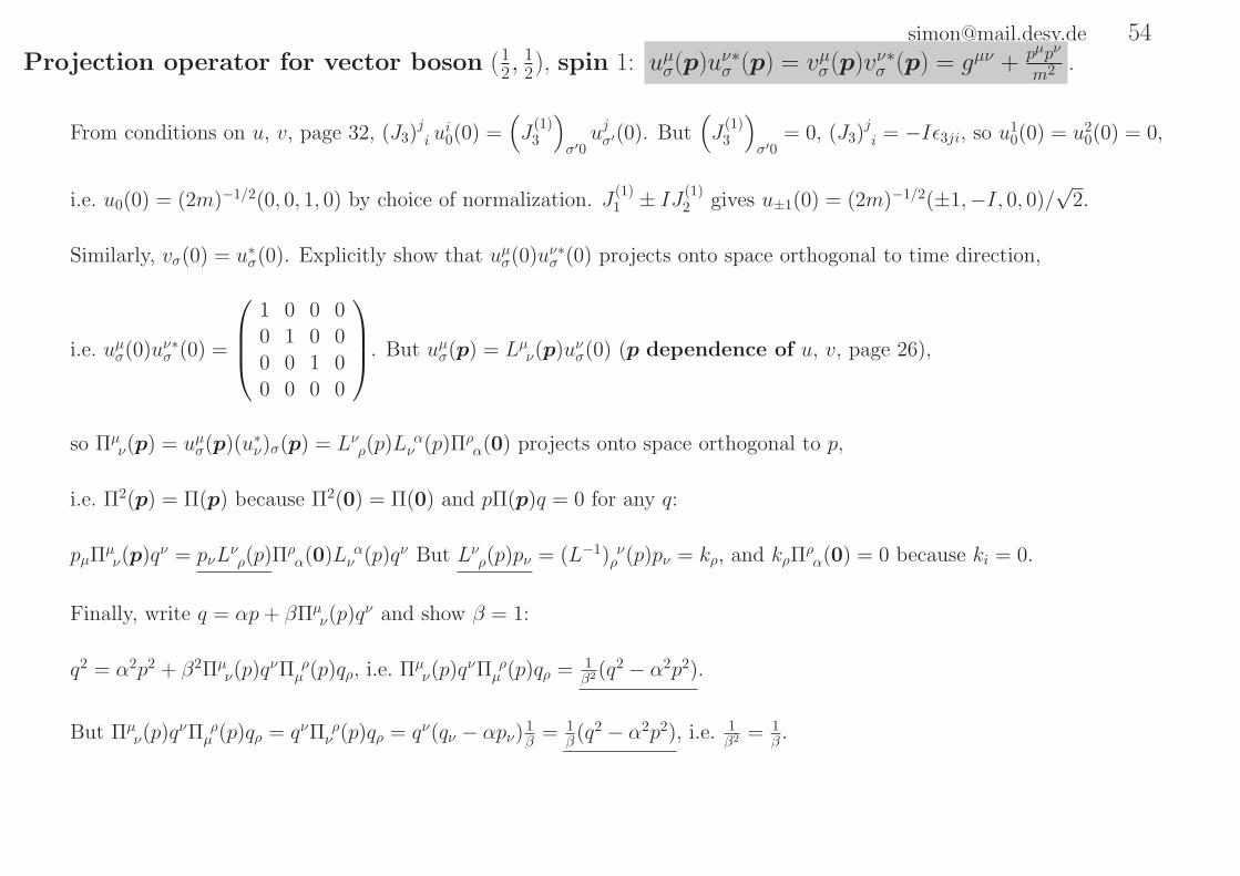
[email protected] 54Projection operator for vector boson (1
2,12), spin 1: uµσ(p)uν∗σ (p) = vµσ(p)vν∗σ (p) = gµν + pµpν
m2 .
From conditions on u, v, page 32, (J3)ji u
i0(0) =
(J
(1)3
)σ′0ujσ′(0). But
(J
(1)3
)σ′0
= 0, (J3)ji = −Iǫ3ji, so u1
0(0) = u20(0) = 0,
i.e. u0(0) = (2m)−1/2(0, 0, 1, 0) by choice of normalization. J(1)1 ± IJ
(1)2 gives u±1(0) = (2m)−1/2(±1,−I, 0, 0)/
√2.
Similarly, vσ(0) = u∗σ(0). Explicitly show that uµσ(0)uν∗σ (0) projects onto space orthogonal to time direction,
i.e. uµσ(0)uν∗σ (0) =
1 0 0 00 1 0 00 0 1 00 0 0 0
. But uµσ(p) = Lµν(p)uνσ(0) (p dependence of u, v, page 26),
so Πµν(p) = uµσ(p)(u∗ν)σ(p) = Lνρ(p)L
αν (p)Πρ
α(0) projects onto space orthogonal to p,
i.e. Π2(p) = Π(p) because Π2(0) = Π(0) and pΠ(p)q = 0 for any q:
pµΠµν(p)qν = pνL
νρ(p)Π
ρα(0)L α
ν (p)qν But Lνρ(p)pν = (L−1) νρ (p)pν = kρ, and kρΠ
ρα(0) = 0 because ki = 0.
Finally, write q = αp+ βΠµν(p)q
ν and show β = 1:
q2 = α2p2 + β2Πµν(p)q
νΠ ρµ (p)qρ, i.e. Πµ
ν(p)qνΠ ρ
µ (p)qρ = 1β2 (q
2 − α2p2).
But Πµν(p)q
νΠ ρµ (p)qρ = qνΠ ρ
ν (p)qρ = qν(qν − αpν)1β = 1
β (q2 − α2p2), i.e. 1
β2 = 1β .
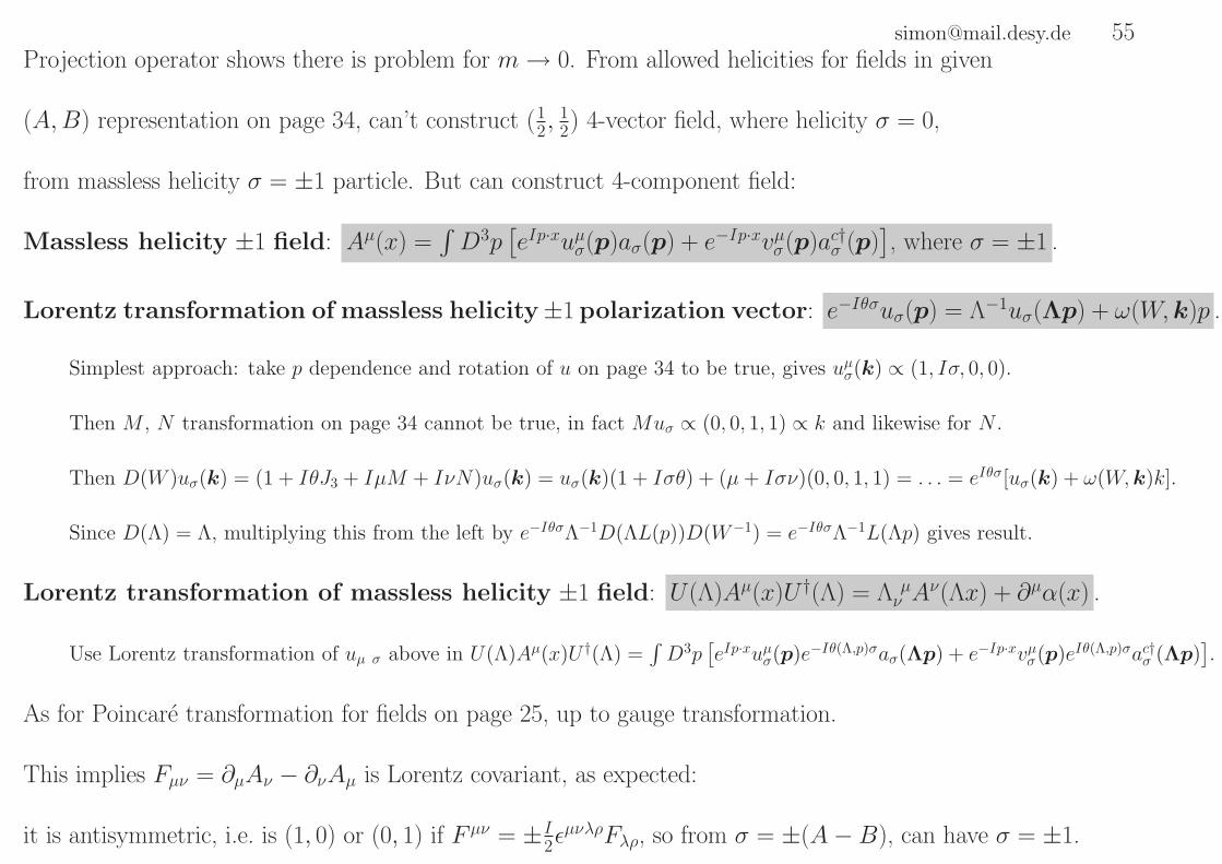
[email protected] 55Projection operator shows there is problem for m→ 0. From allowed helicities for fields in given
(A,B) representation on page 34, can’t construct (12,
12) 4-vector field, where helicity σ = 0,
from massless helicity σ = ±1 particle. But can construct 4-component field:
Massless helicity ±1 field: Aµ(x) =∫D3p
[eIp·xuµσ(p)aσ(p) + e−Ip·xvµσ(p)ac†σ (p)
], where σ = ±1 .
Lorentz transformation of massless helicity±1 polarization vector: e−Iθσuσ(p) = Λ−1uσ(Λp) + ω(W,k)p .
Simplest approach: take p dependence and rotation of u on page 34 to be true, gives uµσ(k) ∝ (1, Iσ, 0, 0).
Then M , N transformation on page 34 cannot be true, in fact Muσ ∝ (0, 0, 1, 1) ∝ k and likewise for N .
Then D(W )uσ(k) = (1 + IθJ3 + IµM + IνN)uσ(k) = uσ(k)(1 + Iσθ) + (µ+ Iσν)(0, 0, 1, 1) = . . . = eIθσ[uσ(k) + ω(W,k)k].
Since D(Λ) = Λ, multiplying this from the left by e−IθσΛ−1D(ΛL(p))D(W−1) = e−IθσΛ−1L(Λp) gives result.
Lorentz transformation of massless helicity ±1 field: U(Λ)Aµ(x)U †(Λ) = Λ µν A
ν(Λx) + ∂µα(x) .
Use Lorentz transformation of uµ σ above in U(Λ)Aµ(x)U †(Λ) =∫D3p
[eIp·xuµσ(p)e−Iθ(Λ,p)σaσ(Λp) + e−Ip·xvµσ(p)eIθ(Λ,p)σac†σ (Λp)
].
As for Poincare transformation for fields on page 25, up to gauge transformation.
This implies Fµν = ∂µAν − ∂νAµ is Lorentz covariant, as expected:
it is antisymmetric, i.e. is (1, 0) or (0, 1) if F µν = ±I2ǫµνλρFλρ, so from σ = ±(A−B), can have σ = ±1.

[email protected] 56Brehmstrahlung: Adding emission of massless helicity ±j boson with momentum q ≃ 0
to process with particles n with momenta pn modifies amplitude by factor ∝ uµ1µ2...µj σ(q)∑
n ηngnp
µ1n p
µ2n ...p
µjn
pn·q ,
where gn is coupling of these bosons to fermion n, and ηn = ±1 for outgoing / incoming particles.
Lorentz invariance condition: qµ1
∑n ηn
gnpµ1n p
µ2n ...p
µjn
pn·q = 0 .
Can show this for massless helicity ±1 boson: Lorentz transformation of polarization vector on page 55
implies amplitude not Lorentz invariant unless this is true.
Einstein’s principle of equivalence: Helicity ±2 bosons have identical coupling to all fermions .
For soft emssion of graviton from process involving multiple fermions of momentum pn,
Lorentz invariance condition reads∑
n ηngnpµ2n = 0. But momentum conservation is
∑n ηnp
µ2n = 0, so gn same for all particles.
Constraint on particle spins: Massless particles must have helicity ≤ 2 and ≥ −2 .
Lorentz invariance condition can be written∑
n ηngnpµ2n . . . p
µjn = 0.
For j > 2 this overconstrains 2 → 2 processes, since momentum conservation alone =⇒ it depends on scattering angle only.

[email protected] 572.6 The Lagrangian Formalism
2.6.1 Generic quantum mechanics
Lagrangian formalism is natural framework for QM implementation of symmetry principles.
Can be applied to canonical fields (e.g. Standard Model):
Fields ψl(x, t) behave as canonical coordinates, i.e. with conjugate momenta pl(x, t) such that
[ψl(x, t), pl′(y, t)]∓ = Iδ3(x − y)δll′ and [ψl(x, t), ψl′(y, t)]∓ = [pl(x, t), pl′(y, t)]∓ = 0 as usual in QM.
In practice, find suitable pl(x, t) by explicit calculation of [ψl(x), ψ†l′(y)]∓.
Lagrangian formalism: Define action A [ψ, ψ] =∫∞−∞ dtL[ψ(t), ψ(t)] , where L is Lagrangian.
Laws of physics obeyed when action is stationary, i.e. coordinates obey field equations ddt∂Ldψl
= ∂L∂ψl
.
Alternatively, define pl = δLδψl
and Hamiltonian H [ψ(t), p(t)] =∫d3x pl(x, t)ψl(x, t) − L[ψ(t), ψ(t)] .
Then action stationary when coordinates obey field equations pl = −δHδψl
.

[email protected] 582.6.2 Relativistic quantum mechanics
Take L[ψ(t), ψ(t)] =∫d3xL (ψ(x), ∂µψ(x)),
where Lagrangian density L (x) is scalar so A =∫d4xL (x) is Lorentz invariant.
In practice, determine L from classical field theory, e.g. electrodynamics,
then L (ψ(x), ∂µψ(x)) = pl(x)ψl(x) − H (ψ(x), p(x)) and pl from L : pl(x) = ∂L (x)
∂ψl(x).
Stationary A requirement gives field equations ∂µ∂L
∂(∂µψl)= ∂L
∂ψl(Euler-Lagrange equations),
e.g. Klein-Gordon equation for free spin 0 field, Dirac equation for free spin 12 field etc.
(some definition of derivative with respect to operator field ψl must be given here).
A must be real. Let A depend on N real fields. Stationary real and imaginary parts of A → 2N field equations.

[email protected] 59Noether’s theorem: Symmetries imply conservation:
A invariant under ψl(x) → ψl(x) + IαFl[ψ;x] → conserved current Jµ(x), ∂µJµ = 0, for stationary A .
If α made dependent on x, A no longer invariant. But change must be δA =∫d4xJµ∂µα
so that δA = 0 when α constant: Ignore l label, use discrete lattice in 1-D of N points so e.g. ψ(x) → ψi and δA =∑
i∂A∂ψiFiαi.
and write ∂A∂ψiFi = (Ji − Ji+1) (no sum) for i = 1, . . . , N − 1, and ∂A
∂ψNFN = (JN −K).
But symmetry of action gives∑
i∂A∂ψiFi = 0, so K = JN+1. (Indices are cyclical, i.e. XN+1 = X1, X0 = XN etc.)
Thus δA =∑
i∂A∂ψiFiαi =
∑i(Ji − Ji+1)αi =
∑i Ji(αi − αi−1). Returning to continuous case, δA =
∫dx δA
δψ(x)F (x) =∫dxJ(x)dαdx .
Thus δA = −∫d4xα∂µJ
µ. Now take A stationary: δA = 0 even though α depends on x, so ∂µJµ = 0.
Explicit result for Noether current when L is invariant: Jµ = ∂L∂∂µψl
Fl .
A =∫d4xL so, for x-dependent α, δA = I
∫d4x
[∂L∂ψl
Flα+ ∂L∂∂µψl
∂µ(Flα)]. But 0 = δL =
(∂L∂ψl
Fl +∂L∂∂µψl
∂µFl
)Iα,
so δA =∫d4xI ∂L
∂∂µψlFl∂µα, then compare with δA =
∫d4xJµ∂µα (from above).
Conserved charge: F =∫d3xJ0 obeys dF
dt = 0.
Use ∂µJµ = 0 and
∫d3x∇J = 0 because J vanishes at infinity.

[email protected] 60Scalar boson (0, 0): Lscalar = −1
2∂µψ∂µψ − 1
2m2ψ2 .
Scalar boson field on page 53 implies[ψ(x, t), ψ(y, t)
]−
= δ(3)(x − y), i.e. p = ψ, consistent with pl from L on page 58.
Field equations on page 58 give Klein-Gordon equation(∂2 −m2
)ψ = 0 as required. Note ψ is a single operator.
Dirac fermion (12, 0) + (0, 1
2): LDirac = −ψ (γµ∂µ +m)ψ .
Recall ψ is a column of 4 operators, and covariant quantities on page 47.
Recall equal time anticommutation relations on page 52, [ψl(x, t), ψ†l′(x, t)]+ = δll′δ
(3)(x − y), so p = ψ†,
consistent with pl from L on page 58. Field equations give Dirac equation (γµ∂µ +m)ψ = 0 as required.
Vector boson (12,
12), spin 1: Lspin 1 vector = −1
4FµνFµν − 1
2m2ψµψ
µ, where Fµν = ∂µψν − ∂νψµ .
From vector boson field and projection operator for vector boson (12 ,
12), spin 1, on pages 53 and 54,
[ψi(x, t), ψj(y, t) + ∂jψ
0(y, t)]−
= δijδ(3)(x − y), i.e. conjugate momentum to ψi is pi = ψi + ∂iψ
0 = F i0,
consistent with pl from L on page 58. ψ0 is auxilliary field because p0 = ∂L∂ψ0
= F00 = 0.
Also ∂µψµ = 0 and Klein-Gordon equation
(∂2 −m2
)ψµ = 0, which is found from field equations on page 58.

[email protected] 612.7 Path-Integral Methods
Follows from Lagrangian formalism. Assume H is quadratic in the pl.
Gives direct route from Lagrangian to calculations, all symmetries manifestly preserved along the way.
Can work in simpler classical limit then return to QM later.
Result is that bosons described by ordinary numbers, fermions by Grassmann variables.
LSZ reduction gives S-matrix from vacuum matrix elements of-time ordered product of functions of fields,
given by path integral as〈0, out|T
ψlA
(xA),ψlB(xB),...
|0, in〉
〈0, out|0, in〉 =∫ ∏
x,l dψl(x)ψlA(xA)ψlB
(xB)...eIA [ψ]
∫ ∏x,l dψl(x)e
IA [ψ] .
Contribution mostly from field configurations for which A is minimal, i.e. fluctuation around classical result.
Noether’s theorem again (see page 59): A invariant under ψl(x) → ψl(x) = ψl(x) + IαFl[ψ;x].
So if α dependent on x,∫ ∏
x,l dψl(x) exp[IA ] →∫ ∏
x,l dψl(x) exp[I(A −
∫d4x∂µJ
µ(x)α(x))]
assuming measure∏
x,l dψl(x) invariant. This is just change of variables, so 〈∂µJµ(x)〉 = 0.

[email protected] 622.8 Internal symmetries
Consider unitary group representations.
Unitary U(N): elements can be represented by N ×N unitary matrices U (U †U = 1).
Dimension d(U(N))= N 2.
2N 2 degrees of freedom in complex N ×N matrix, U †U = 1 is N 2 conditions
or N 2 Hermitian N ×N matrices: N diagonal reals, N 2 −N off-diagonal complexes but lower half conjugate to upper.
Special unitary SU(N): same as U(N) but U ’s have unit determinant (det(U) = 1).
Thus tr[ti] = 0, i.e. group is semi-simple.
d(SU(N))= N 2 − 1.
Fundamental representation denoted N .
Normalization of fundamental representation: tr[titj] = 12δij (i.e. C(N ) = 1
2).

[email protected] 63U(1) (Abelian group): elements can be represented by phase eIqα.
One generator: the real number q (the charge).
SU(2): Fundamental representation denoted 2, spin 12 representation of rotation group.
SU(2) is actually the universal covering group of rotation group. 3 generators ti = σi2 , [ti, tj] = Iǫijktk.
Adjoint representation denoted 3. C(3) = 2.
ǫjkiǫlki = (d(SU(2)) − 1)δjl = 2δjl.
2 representation is real, 2 = 2 (i.e. −σ∗i2 = U σi
2 U†, pseudoreal), and gαβ = ǫαβ and δαβ.
SU(3): 8 generators λi2 , structure constants fijk.
Fundamental representation 3: λi are 3 × 3 Gell-Mann matrices. Adjoint representation 8. C(8) = 3.
3 representation is complex, 3 6= 3.
Example: 3 × 3 = 8 + 1, i.e. quark and antiquark can be combined to behave like gluon or colour singlet.

[email protected] 642.8.1 Abelian gauge invariance
Global gauge invariance: Consider complex fermion / boson field ψl(x), arbitrary spin.
Each operator in Lfree is product of (∂µ)ψl with (∂µ)ψ†l ,
invariant under U(1) transformation ψl → eIqαψl (whence ∂µψl → eIqα∂µψl)
if α independent of spacetime coords.
Local gauge invariance: Find L invariant when α = α(x). Leads to renormalizable interacting theory.
In Lfree, ∂µψl → ∂µeIqαψl = eiqα
[∂µψl + Iq(∂µα)ψl
]6= eIqα∂µψl, ∴ replace ∂µ by 4-vector “derivative” Dµ,
such that Dµ gauge transformation Dµψl → eIqαDµψl . Then Dµψl(Dµψl)
† invariant.
Simplest choice: Dµ − ∂µ is 4-component field:
Covariant derivative: Dµ = ∂µ − IqAµ(x) .
Gauge transformation: Aµ → Aµ + ∂µα whenever ψl → eIqαψl .
Write transformation as Aµ → A′µ(α). Require Dµψl → D′
µeiqαψl = eiqαDµψl,
i.e. eIqα[∂µψl − Iq(∂µα)ψl − IqA′
µψl]
= eIqα [∂µψl − IqAµψl], so A′µ = Aµ + ∂µα.

[email protected] 65Use Dν to find invariant (free) Lagrangian for Aµ, quadratic in (∂ν)Aµ:
From Dµ gauge transformation, DµDν . . . ψl → eIqαDµDν . . . ψl. Products DµDν . . . contain spurious ∂ρs, but
Fµν from Dµ: qFµν = I [Dµ, Dν], where electromagnetic field strength Fµν = ∂µAν − ∂νAµ .
[Dµ, Dν]ψl =([∂µ, ∂ν]︸ ︷︷ ︸
=0
+Iq([∂µ, Aν] − [∂ν, Aµ]) − q2 [Aµ, Aν]︸ ︷︷ ︸=0
)ψl.
Fµν is gauge invariant.
Fµνψl → F ′µνe
Iqαψl = eIqαFµνψl, i.e. F ′µν = Fµν, or Fµν → Fµν. Also check explicitly from Fµν = ∂µAν − ∂νAµ.
Conversely, choose Aµ to be massless helicity ±1 field, whose Lorentz transformation on page 55
implies Lorentz invariant free Lagrangian for Aµ must be gauge invariant.
Fµν in representation of U(1): Since Fµν → Fµν, Fµν transforms in adjoint representation of U(1).
Example: QED Lagrangian for fermions: LDirac, QED = −ψ (γµDµ +m)ψ︸ ︷︷ ︸LDirac, free+Iqψγ
µAµψ
−14FµνF
µν.
Interactions due to IqψγµAµψ. Most general Lagrangian locally gauge invariant under U(1) (ψ → eIqαψ, Aµ → Aµ + ∂µα),
assuming P, T invariance and no mass dimension > 4 terms (Wilson: no contribution).

[email protected] 662.8.2 Non-Abelian gauge invariance
Global gauge invariance: Each term in Lfree proportional to (∂µ)ψl γ(∂µ)ψ†l′ γ, γ = 1, . . . , N .
Then Lfree invariant under ψl γ → Uγδψl δ , where U = exp[Iαiti] , αi spacetime independent.
So ψγ is in fundamental representation of group G =SU(N) formed by matrices Uγδ, i = 1, . . . , d(G).
Local gauge invariance: Spacetime derivatives in Lagrangian appear as
Covariant derivative: Dµ = ∂µ − IAµ(x) with Aµ = Aµi ti,
ti contain couplings, Aµi for i = 1, . . . , d(G) are (for) massless helicity ±1 gauge fields.
To achieve Dµψ → UDµψ, require
Transformation of covariant derivative: Dµ → UDµU† , which requires
Transformation of gauge fields: Aµ → UAµU† − I (∂µU)U † .

[email protected] 67Non-Abelian field strength: TiF
iµν =Fµν = I [Dµ, Dν] = ∂µAν − ∂νAµ − I [Aµ, Aν] .
Fµν in adjoint representation: Fµν → UFµνU† .
In infinitesimal case, F iti αβ → F i [(1 + Iαktk)ti(1 − Iαktk)]αβ = F i [ti + Iαk [tk, ti]]αβ
= F i [ti + Iαk(ICkij)tj]αβ = F i[ti αβ + Iαk(t
kji)tj αβ
]= F itj αβ
[δji + Iαk(t
kji)]
= F itj αβUji = UijFjti αβ, i.e. F i → UijFj.
Example: QCD Lagrangian for fermions:LDirac, QCD = −ψα (γµDαβ µ +m)ψβ − 14F
iµνF
i µν.
More general result is −14gijF
iµνF
j µν, but can always diagonalize and rescale so gij → δij.

[email protected] 682.9 The Standard Model
Symmetry of vacuum is G=SU(3)colour×U(1)e.m. gauge group.
SM: At today’s collider energies, some “hidden” (broken) symmetries become apparent:
G=SU(3)colour×SU(2)weak isospin×U(1)weak hypercharge.
Table 2.9.1: SM fermions and their SU(3)C×SU(2)L×U(1)Y representations, written as (SU(3)C rep.,SU(2)L rep.,U(1)Y hyper-charge = generator / [coupling ≡ Y ]). The SU(3)C charges (3 for quarks, none for leptons) are not shown but, since SU(2)Lis broken, particles differing only in T3 (component of weak isospin SU(2)L) are shown explicitly, namely uL / νe (T3 = 1/2)and dL / eL (T3 = −1/2). Recall ψL/R = 1
2(1 ± γ5)ψ. Note e.g. uL annihilates u−L and creates u+R, and νe is left-handed.
Names Label Representation under SU(3)C×SU(2)L×U(1)Y
Quarks QL = (uL, dL) (3,2, 1
6)
u†R (3,1,−2
3)
d†R (3,1, 1
3)
Leptons EL = (νe, eL) (1,2,−1
2)
e†R (1,1, 1)
Gauge fields are written as
SU(3): gµ = giµ gsλi2
SU(2): Aµ = Aiµ gσi2
U(1): Bµ = Bµ g′Y .

[email protected] 69We have only discussed the “1st generation” of fermions, in fact (EL, e
†R,QL, u
†R, d
†R)K , K = 1, 2, 3.
where (e1, e2, e3) = (e, µ, τ ), (ν1e , ν
2e , ν
3e ) = (νe, νµ, ντ ), (u1, u2, u3) = (u, c, t) and (d1, d2, d3) = (d, s, b).
Allow mixing between particles of different generations with same transformation properties.
From Table 2.9.1, can construct the full Lagrangian by including all renormalizable invariant (1,1, 0) terms.
These are all possible terms of form ψKγµDµψ
K :
Lquark = QK
L γµ[∂µ − I(gµ + Aµ + Bµ)]QK
L + uKRγµ[∂µ − I(gµ + Bµ)]u
KR + d
K
Rγµ[∂µ − I(gµ + Bµ)]d
KR .
Llepton = EK
L γµ[∂µ − I(Aµ + Bµ)]E K
L + eKRγµ[∂µ − IBµ]e
KR .
More general ψKγµDµR
KMψM for some constant matrix R not allowed, gives terms ψKγµ∂µψ
M for K 6= M .
Lspin 1 = −14F
iµν(g)F
i µν(g) − 14F
iµν(A)F i µν(A) − 1
4Fµν(B)F µν(B).
Recall only real part of L to be taken.

[email protected] 702.9.1 Higgs mechanism
Mass terms mψL/RψR/L are all (1,2,±12) → violate gauge symmetry and thus renormalizability.
Instead introduce Yukawa coupling λφHψL/RψR/L which is (1,1, 0), i.e. invariant (thus renormalizable),
so φH is (1,2 = 2, 12) scalar field, then hide (“break”) symmetry so that λ〈0|φH|0〉 = m.
LHiggs = Lpure Higgs + LHiggs−fermion .
Writing Dµ = ∂µ− I(Aµ+ Bµ) and SU(2)L components φTH = (φH 1, φH 2) = (φ+H , φ
0H), (ǫφ†H)T = (φ0†
H ,−φ+†H ),
Lpure Higgs = −12(DµφH)†DµφH − V (φH) , Higgs potential V (φH) =
m2H2 φ
†HφH + λ
4(φ†HφH)2
LHiggs−fermion = −GKMe E
K
L aφH aeMR −GKM
u QK
L a(ǫφH)†auMR −GKM
d QK
L aφH adMR .
All three terms are (1,1, 0), i.e. invariant. Consider e.g. second term: From table 2.9.1, Y = −16 − 1
2 + 23 = 0.
Write SU(2)L transformation of φH as φ′H a = UabφH b (U = eI12σiαi from page 63),
so (ǫφ′H)†a = (ǫφH)†bU−1∗ba from ǫacσcdǫ
Tdb = −σ∗ab. (Same transformation as φTH : φ′H a = φH bU
Tba = φH bU
−1∗ba .)
Also Q′L a = UabQL b, so Q′†
L a = U ∗acQ
†L c, so Q′†
L a(ǫφ′H)†a = Q†
L a(ǫφH)†a. Note uR is an SU(2)L singlet.

[email protected] 71m2H > 0: Stationary L (vacuum) occurs when all fields vanish.
Spontaneous symmetry breaking (SSB): m2H < 0: tree level vacuum obeys ∂V (φH)
∂φ
∣∣φH=φH0
= 0
=⇒ |φ2H0| = v2 =
|m2H |λ . From Higgs potential on page 70.
Infinite number of choices for φ0H = 〈0|φH |0〉. Take general φH = eIvξi(x)σi2
(0
v + η(x)
).
Vacuum taken as ξi = η = 0, no longer invariant under symmetry transformations.
Lgauge mass = −m2WW
†µW
µ − 12m
2ZZµZ
µ , where mZ = v2
√g2 + g′2 , mW = v
2g = mZ cos θW , cos θW = g√g2+g′2
,
Wµ = 1√2(A1 µ − IA2 µ) , Zµ = cos θWA3 µ − sin θWBµ .
From Lpure Higgs. Start with Lgauge mass = −12
∣∣∣∣(gAi µ
σi2 + g′Bµ
12
)( 0v
) ∣∣∣∣2
= −12
∣∣∣∣(g(A1 µ + IA2 µ)−gA3 µ + g′Bµ
)v2
∣∣∣∣2
.
Lgauge dynamic = −12|∂µW ν − ∂νW µ|2 − 1
4|∂µZν − ∂νZµ|2 − 14|∂µAν − ∂νAµ|2 ,
where Aµ = sin θWA3 µ + cos θWBµ must be massless photon.
From Lspin 1. Start with Lgauge dynamic = −14|∂µAν
i − ∂νAµi |2 − 1
4|∂µBν − ∂νBµ|2.

[email protected] 72In Lquark and Llepton on page 69, between left-handed fermions:
(Aµ + Bµ)L =
(e(
12 + Y
)Aµ +
(g2 cos θW − g′Y sin θW
)Zµ
g√2W †
µg√2Wµ e
(−1
2 + Y)Aµ +
(−g
2 cos θW − g′Y sin θW)Zµ
),
between right-handed: (Aµ + Bµ)R = eY Aµ + (−g′ sin θWY )Zµ , where e = g sin θW = g′ cos θW .
So charge/e is Q = T3 + Y , i.e. charge of uL, dL, νe, eL is 23, −1
3, 0, −1 and of uR, dR, eR is 23, −1
3, −1.

Lfermion mass = −eKLmKMe eMR − uKLm
KMu uMR − d
K
LmKMd dMR , where mKM
ψ = GKMψ v .
From LHiggs−fermion on page 70.
Can always transform uK′R = AKM
uRuMR , likewise for uL, dL, dR, νe, eL, eR.
A matrices must be unitary so that kinetic terms retain their previous forms, uK′R γ
µ∂µuK′R etc.
Choose A matrices such that new mass matrices m′u = AuLmuA
†uR
etc. diagonal, entries mK′u :
Lfermion mass =∑
K −eK′L m
Ke e
K′R − uK′
L mK′u u
K′R − d
K′L m
K′d d
K′R .
Then LW −fermion ∝ dK
L γµWµu
KL + eKL γ
µWµνKe = d
K′L γ
µWµ(V†)KNuN ′
L + eK′L γ
µWµνK′′e
(proportionality constant is − Ig√2), where CKM matrix V = AuLA
−1dL
.
Analogous leptonic matrix absorbed into νK′′e =
(AeLA
−1νe
)KNνN ′e .
(In contrast to uKL , any combination of νKe is mass eigenstate because mass matrix is zero.)

[email protected] 742.9.2 Some remaining features
Neutrino mass by adding to LHiggs−fermion a term −GνeEK
a (ǫφH)†aνeR → −νemνeνeR, where νeR is (1,1, 0).
Expect mνe ∼ v to be similar order of magnitude to quark and charged lepton masses.
Also allowed SM invariant term −12ν
TeRMRνeR, can only come from higher scale symmetry breaking,
so MR ≫ v ∼ mνe, i.e. no right handed neutrinos at low energy.
Gives Lneutrino mass = −12(νe νTeR)
(0 mνe
mνe MR
)(νTeνeR
)≃ −1
2(ν′e ν ′TeR)
(−m2
νeMR
0
0 MR
)(ν ′Teν ′eR
),
i.e. seesaw mechanism: massm2νe
MRof (almost) left handed ν ′e (i.e. mνe suppressed by
mνeMR
).

[email protected] 75Invariance with respect to parity P , charge conjugation C and time reversal T transformations.
CPT conserved, but CP -violation due to phases in CKM matrix.
CP and P violating terms θ64π2ǫ
κλρσF iκλF
iρσ allowed, but are total derivatives and therefore non-perturbative.
Current observation suggest θ consistent with zero (no CP violation in QCD).
Cancelled by (harmless) anomaly (subsubsection 2.9.4) of global symmetry ψf → eIγ5αfψf when∑αf = −1
2θ,
but this introduces unobserved CP violating phase e−Iθ on quark masses.
Peccei-Quinn mechanism: where (ǫφH)† in LHiggs−fermion on page 70 is replaced with second Higgs,
which transforms differently to first Higgs and can soak up this phase at least at some GUT scale.

[email protected] 762.9.3 Grand unification
Suppose SM unifies to single group G at scale MX , then tU(1)Y (diagonal), tSU(2)Li , t
SU(3)Cj are generators of G.
Tracelessness requires sum of Y values (=elements of tU(1)Y ) to vanish, which is the case from Table 2.9.1.
Normalization of generators as on page 14, so tr[tU(1)Y 2] =tr[tSU(2)L2i ] =tr[t
SU(3)c2j ], so
g2s(MX) = g2(MX) = 5
3g′2(MX) (after dividing by 2×no. generations). Implies sin2 θW (MX) = 3
8 from page 71.
Within couplings’ exp. errors, unification occurs (provided N = 1 SUSY is included) at MX = 2 × 10¹⁶ GeV.
To find simplest unification with no new particles, note SM particles are chiral, require complex representations:
In general, define all particles fL to be left-handed, then antiparticles fR = f †L are right-handed.
Then if fL in representation R of some group G, fR is in representation R.
If fL, fR equivalent (have same transformation properties), then R = R, i.e. pseudoreal representation.
SM particles fL = (EL, e†R,QL, u
†R, d
†R) require complex representation because fR = f †L inequivalent, e.g. 3 6= 3.
Pseudoreal representation possible if particle content enlarged to fL → FL so that FL, FR = F †L equivalent.
e.g. in SO(10), can fit 15 particles of each generation into real 16 representation, requires adding 1 νeR.

[email protected] 77SU(5) is simplest unification.
Since SU(3)×SU(2)×U(1) ⊂ SU(5), all internal symmetries accounted for by fermions ψα with α = 1, ..., 5.
Choose tSU(3)i = gs
0 0λi2 0 0
0 0
0 0 0 0 0
0 0 0 0 0
= tSU(3)Ci , i = 1, ..., 8, t
SU(2)i = g
0 0 0 0 0
0 0 0 0 0
0 0 0 0 0
0 0 0 σi20 0 0
= tSU(2)Li , i = 1, ..., 3.
U(1) generator must commute with generators above and be traceless. Tentatively take
tU(1) = 2g′
13 0 0 0 0
0 13 0 0 0
0 0 13 0 0
0 0 0 −12 0
0 0 0 0 −12
= 2tU(1)Y .
Then fermions form 5 (fundamental) and 10 representations of SU(5):
d1
R
d2
R
d3
R
eL−νeL
,
0 u3R −u2
R u1L d1
L
0 u1R u2
L d2L
0 u3L d3
L
—“0 eR
0
.
(Note: all particles left-handed, 1,2,3 superscripts are colour indices, 10 matrix is antisymmetric).
In SO(10), 1 generation fits into 16 = 1 + 5 + 10, and 1 is identified with right-handed neutrino.

[email protected] 782.9.4 Anomalies
Gauge anomalies modify symmetry relations (Ward identities), spoils renormalizability and maybe unitarity.
Anomaly occurs because A =∫d4xL respects symmetry, but not measure
∫ ∏x,l dψl(x) = d[ψ]d[ψ]d[A].
Relevant example: Let A be invariant under ψα = Uk αβψβ,
where Uk = exp[Iγ5αtk] is chiral symmetry (global) and each ψα is a Dirac field.
Problem: although A is invariant, measure is not: Resulting change in path-integral∫d[ψ]d[ψ]d[A] exp[IA ]
is “as if” L changes by αJk[A], where Jk = − 116π2ǫµνρσF
µνi F ρσ
j tr[ti, tjtk].
Noether’s theorem on page 61:∫d[ψ]d[ψ]d[A] exp[IA ] →
∫d[ψ]d[ψ]d[A] exp[I
(A +
∫d4xα(x) [Jk − ∂µJ
µk (x)]
)],
i.e. conservation violation: 〈∂µJµk (x)〉A = − 116π2ǫµνρσF
µνi F ρσ
j tr[ti, tjtk] (〈〉A means no A integration).
Anomalous (non-classical) triangle diagrams between Jµk , F µνi and F ρσ
j modify Ward identities.
Physical theories must be anomaly free (i.e. tr[ti, tjtk] cancel), e.g. real representations: tr[ti, tjtk] = 0.
tr[t∗i , t∗jt∗k] =tr[(−UtiU †), (−UtjU †)(−UtkU †)] = −tr[ti, tjtk]. But tr[t∗i , t∗jt∗k] =tr[tTi , tTj tTk ] =tr[ti, tjtk].
SM is anomaly free. SM in 10 + 5 of SU(5), in real representation 16 of SO(10) (thus tr[ti, tjtk]5 = −tr[ti, tjtk]10).

[email protected] 793 Supersymmetry: development
3.1 Why SUSY?
Attractive features of SUSY:
1. Eliminates fine tuning in Higgs mass.
2. Gauge coupling unification.
3. Radiative electroweak symmetry breaking: SUSY =⇒ Higgs potential on page 70 with m2H < 0.
4. Excess of matter over anti-matter (large CP violation, not in SM) possible from SUSY breaking terms.
5. Cold dark matter may be stable neutral lightest SUSY particle (LSP) = gravitino / lightest neutralino.
6. Gravity may be described by local SUSY = supergravity.

[email protected] 80SM is accurately verified but incomplete — e.g. does not + cannot contain gravity,
so must break down at / before energies around Planck scale MP = (8πG)−1/2 = 2.4 × 10¹⁸ GeV.
In fact, SM cannot hold without modification much above 1 TeV, otherwise we have
Gauge hierarchy problem: Since v = |〈0|φH |0〉| = 246GeV and λ = O(1), |mH | = |√λv| = O(100) GeV .
If ΛUV > O(1)TeV, fine tuning between
∆m2H from quantum loop corrections (Fig. 3.1) and tree level (bare) m2
H :
∆m2H =
λφ8π2Λ
2UV − 3︸︷︷︸
colour“3′′
|κt|28π2 Λ2
UV + ...︸︷︷︸smaller terms
.
φH
ψ
(a) Fermion field ψ, Lagrangian term −κψφHψψ, giving 1-loop contribution to
Higgs mass of − |κψ|2
8π2 Λ2UV.
φH
φ
(b) Boson field φ, Lagrangian term λφ|φH |2|φ|2, giving 1-loop contribution to
Higgs mass ofλφ8π2 Λ2
UV.
Figure 3.1: Fermion and boson contributions to Higgs mass parameter m2H .
(Largest from −λφ4 |φH|4 and top quark (κt ≃ 1 because mt ≃ v).)
No similar problem for fermion and gauge boson masses, but these masses affected by m2H .

[email protected] 81Avoid fine tuning by taking ΛUV ∼ 1 TeV, i.e. modify SM above this scale.
One solution: Higgs is composite of new fermions bound by new strong force at ΛUV ≃ 1 TeV → difficult.
Alternatively, forbid bare m2H|φH|2 term by some new symmetry δφH = ǫ × something.
Various choices for “something” bosonic (leads to “little Higgs” models, extra dimensions).
For a standard symmetry, “something” would be I [Qa, φH ], i.e. φH → eIǫQaφHe−IǫQa.
Try “fermionic” generator Qa, which must be a(
12, 0)
spinor (so ǫ a spinor of Grassmann variables).

[email protected] 82Relation with momentum: Qa, Q
†b = 2σµ
abPµ .
Qa, Q†b is
(12 , 0)×(0, 1
2
)=(
12 ,
12
)from triangle inequality. Only candidate is P µ (see Coleman-Mandula theorem later).
Lorentz invariance requires combination σµabPµ, factor 2 comes from suitable normalization of Qa.
Note Qa, Q†b 6= 0 because for any state |X〉,
〈X|Qa, (Qa)†|X〉 = 〈X|Qa (Qa)
† |X〉 + 〈X| (Qa)†Qa|X〉 =
∣∣ (Qa)† |X〉
∣∣2 +∣∣Qa|X〉
∣∣2 ≥ 0. If equality holds for all |X〉, Qa = 0.
At least one of Pµ non-zero on every state, so Qa affects every state, not just Higgs,
i.e. every particle has a superpartner with opposite statistics and spin difference of 1/2,
together called a supermultiplet. This fermion-boson symmetry is supersymmetry.
For every fermion field (component) ψf with −κfφHψfψf , introduce boson field φf with −λf |φH|2|φf |2.
From Fig. 3.1, contribution of this supermultiplet (component) to ∆m2H is ∆m2
H =λf8π2
Λ2UV
︸ ︷︷ ︸boson
−|κf |28π2
Λ2UV
︸ ︷︷ ︸fermion
.
Just requiring fermion-boson symmetry guarantees λf = |κf |2, and ∆m2H = 0 (+ finite terms) to all orders.

[email protected] 833.2 Haag-Lopuszanski-Sohnius theorem and SUSY algebra
Reconsider symmetries: So far assumed generators are bosonic. Now generalize to include fermionic ones.
Generalize additive observable on page 5 to Q = Qσσ′a†σaσ′.
(If Qσσ′ are components of Hermitian matrix, unitary transformation of particle states gives back original result.)
Since Q is bosonic, a†σ, a†σ′ both bosons or both fermions, i.e. Qσσ′ = 0 if a†σ bosonic, a†σ′ fermionic, or vice versa.
SUSY: Allow forQ’s containing fermionic parts to also be generators of symmetries that commute with S-matrix.
For convenience, distinguish between fermionic and bosonic parts of any Q.
Fermionic Q = Qσρa†σaρ +Rσρa
†ρaσ, where σ sums over bosonic particles, ρ over fermionic particles.
Such a generator converts bosons into fermions and vice versa.
E.g. action of Q on 1 fermion + 1 boson state using (anti) commutation relations on page 4 gives
Qa†ρ′a†σ′|0〉 = Qσρ′a
†σa
†σ′|0〉 +Rσ′ρa
†ρa
†ρ′|0〉.
But as a symmetry implies there are fermions and bosons with similar properties.

[email protected] 84Identify symmetry generators ti also with fermionic Q.
Graded parameters αi, βj obey αiβj = (−1)ηiηjβjαi, where grading ηi = 0(1) for complex (Grassmann) αi.
Graded generator tj obeys αitj = (−1)ηiηjtjαi, where ηi = 0(1) for bosonic (fermionic) generator ti.
For transformations O → eIαitiOe−Iαiti to preserve grading of any operator O , αi has same grading as ti.
Graded Lie algebra: [(−1)ηiηjtitj − tjti] = ICijktk .
Repeating steps in derivation of Lie algebra on page 8 gives
12ICijkαiβjtk = 1
2 [αitiβjtj − βjtjαiti] = 12 [(−1)ηiηjαiβjtitj − αiβjtjti].
Fermionic generators Qi: U(Λ)QiU†(Λ) = Cij(Λ)Qj, so Qi furnishes representation of Lorentz group.
Choose Qi = Q(A,B)ab in (A,B) representation: [A, Q
(A,B)ab ] = −J
(A)aa′ Q
(A,B)a′b and [B, Q
(A,B)ab ] = −J
(B)bb′ Q
(A,B)ab′ .
Anticommutators of fermionic generators can be used to build bosonic generators of various (A,B).
Coleman-Mandula theorem puts limits on allowed bosonic generators, and hence allowed (A,B) for the Q(A,B)ab .

[email protected] 85Coleman-Mandula theorem: Only bosonic generators are of internal + Poincare group symmetries.
Simple argument: Additional conserved additive rank ≥ 1 tensors constrain scattering amplitude too much.
Only 1 4-vector, P µ: Consider 2→2 scattering, c.m. frame.
Conservation of momentum and angular momentum → amplitude depends on scattering angle θ.
Second conserved additive 4-vector Rµ gives additional constraints unless Rµ ∝ P µ.
Only 1 2nd rank tensor, Jµν: Assume rank 2 conserved additive tensor Σµν.
Additive property means [Σµν, a†σ(p)] = Cµν σ(p)a†σ(p). Then Cµν(p, σ) = ασ(m
2)pµpν + βσ(m2)gµν.
Lorentz transformation of RHS is U(Λ)[Σµν, a†σ(p)]U †(Λ) = [U(Λ)ΣµνU
†(Λ), U(Λ)a†σ(p)U †(Λ)]
= [ΛρµΛ
δνΣρδ, Dσ′σ(W (Λ, p))a†σ′(Λp)] = Dσ′σ(W (Λ, p))Λρ
µΛδνCρδ(Λp, σ)a†σ′(Λp),
and of LHS is Cµν(p, σ)Dσ′σ(W (Λ, p))a†σ′(Λp), so Λ ρµ Λ δ
ν Cρδ(p, σ) = Cµν(Λp, σ). Only candidates are pµpν and gµν.
In 2→2 scattering, conservation of Σµν implies ασ1(m21)p
µ1p
ν1 + ασ2(m
22)p
µ2p
ν2 = ασ1(m
21)p
′µ1 p
′ν1 + ασ2(m
22)p
′µ2 p
′ν2 .
P µ conservation: pµ1+pµ2 = p′µ1 +p′µ2 =⇒ pµ1,2 = p′µ1,2, i.e. no scattering (allowed pµ1,2 = p′µ2,1 if ασ1(m21) = ασ2(m
22)).
No higher rank tensors: Generalize last argument to higher rank tensors.

[email protected] 86Allowed representations for fermionic generators Q
(A,B)ab : A +B = 1
2 , i.e.(
12, 0)
or(0, 1
2
), and j = 1
2.
Q(C,D)C,−D, Q
(C,D)†C,−D = X
(C+D,C+D)C+D,−C−D : Firstly, Q(C,D)† is of type (A,B) = (D,C) because B† = A.
Writing Q(C,D)†C,−D = Q
(D,C)a,b , we find b = −C because [B−, Q
(D,C)a,b ] = −[A+, Q
(C,D)C,−D]† = 0 using B− = A†
+. Similarly a = D.
Now Q(C,D)C,−D, Q
(C,D)†C,−D = Q(C,D)
C,−D, Q(D,C)D,−C, must have A3 = C +D and B3 = −C −D, i.e. A,B ≥ C +D.
But since A must be ≤ (C +D) (from triangle inequality), it must be = C +D. Similarly for B.
Since X(C+D,C+D) is bosonic, CM theorem means it must be P µ ((
12 ,
12
)), or internal symmetry generator ((0, 0)).
Latter implies C = D = 0, not possible by spin-statistics connection. Final result is relation with momentum on page 82.
Take Qa to be(
12, 0)
spinor, i.e. [A, Qa] = −12σabQb , [B, Qa] = 0 (Q†
a will be(0, 1
2
)).
Qa not ruled out by reasoning of CM theorem, because no similar conservation law:
Take |i〉, |j〉 to have definite particle number. 〈j|i〉 6= 0 =⇒ even difference in fermion numbers, so 〈j|Qa|i〉 = 0.
Can have multiple generators Qar, r = 1, ..., N −→ simple SUSY is N = 1, extended SUSY is N ≥ 2.
Summary:
CM theorem: only bosonic generators are (0, 0) (internal symmetry),(
12,
12
)(P µ), and (1, 0) and (0, 1) (Jµν).
HLS theorem: only fermionic generators are(
12, 0)
and(0, 1
2
)(Qar).

[email protected] 87Relation with momentum for any N : Qar, Q
†bs = 2δrsσ
µ
abPµ .
From allowed representations for fermionic generators on page 86, Qar, Q†bs = 2Nrsσ
µ
abPµ. Nrs is Hermitian,
because Qar, Q†bs† = Qbs, Q
†ar = 2N ∗
rsσµbaPµ, but Qbs, Q
†ar = 2Nsrσ
µbaPµ. So N diagonalized by unitary matrix W .
Writing Q′ar′ = Wr′rQar gives Q′
ar, Q′†bs = 2nrδrsσ
µ
abPµ (no sum over r on RHS), where nr are eigenvalues of Nrs.
Writing Qar = Q′ar/
√nr gives result if nr > 0 (otherwise we have a factor -1):
Taking Q′†bs
= (Q′ar)
† and operating from right and left with |X(p)〉 and 〈X(p)| where Q′ar|X(p)〉 6= 0 gives
on LHS: 〈X(p)|Q′ar, (Q
′ar)
†|X(p)〉 = | (Q′ar)
†|X(p)〉|2 + |Q′ar|X(p)〉|2 > 0, and
on RHS: 2nr(p0 ± p3), where ± for a = 1, 2. If p0 ≥ ∓p3, then nr > 0 as required.
SUSY implies 〈0|H|0〉 = 0 for supersymmetric vacuum (Qar|0〉 = Q†ar|0〉 = 0).
Commutation with momentum: [Qa, Pµ] = 0 .
[Qa, Pµ] is
(12 , 0)×(
12 ,
12
)=(1, 1
2
)+(0, 1
2
). No
(1, 1
2
)generator, but Q†a is
(0, 1
2
).
So [Qb, Pµ] = kσµbaQ
†a and therefore[Q†a, P
µ]
= −k∗Qbσµba, or, using ǫ matrix,[Q†a, P µ
]= k∗σµ abQb.
Jacobi identity: 0 = [[Qa, Pµ], P ν] + [[P µ, P ν], Qa] + [[P ν, Qa], P
µ] = kσµab
[Q†b, P ν] − kσνab
[Q†b, P µ] = |k|2[σµ, σν] ba Qb.
Since [σµ, σν] ba 6= 0 for all µ, ν, must have |k|2 = k = 0.

[email protected] 88Anticommuting generators: Qar, Qbs = ǫabZrs , with (0, 0) generators Zrs = −Zsr.
Qar, Qbs is (1, 0) + (0, 0). From CM theorem, only (1, 0) generator is Jµν. But [Qar, Qbs, P µ] = 0 (commutation with
momentum, page 87), while (linear combinations of) Jµν doesn’t commute with P µ (see Poincare algebra, page 21).
So only possibility is (0, 0) generators, which in general commute with P µ from CM theorem.
Lorentz invariance requires ǫab(= −ǫba), but whole expression symmetric under ar ↔ bs so Zrs = −Zsr.
Antisymmetry of Zrs → vanish for N = 1. Zrs are central charges due to following commutation relations:
Commutation with central charges: [Zrs, Qat] = [Zrs, Q†at] = 0 .
Jacobi identity 0 = [Qar, Qbs, Q†ct] + [Qbs, Q
†ct, Qar] + [Q†
ct, Qar, Qbs].
2nd, 3rd terms vanish from commutation with momentum on page 87. Thus [Zrs, Q†at] = 0.
Jacobi identity 0 = −[Zrs, Qat, Q†bu] + Q†
bu, [Zrs, Qat] − Qat, [Q
†bu, Zrs].
1st, 3rd terms vanish because Zrs commutes with P µ and Q†bu
.
Commutator in 2nd term must be [Zrs, Qat] = MrstvQav, so 0 = Q†bu, [Zrs, Qat] = 2Mrstuσ
µ
abPµ, i.e. Mrstu = 0 so [Zrs, Qat] = 0.
Commuting central charges: [Zrs, Ztu] = [Zrs, Z†tu] = 0 . [Zrs, Ztu] = [Q1r, Q2s, Ztu] = 0, etc.
R-symmetry: Zrs = 0 gives U(N) symmetry Qar → VrsQas (N = 1 case: Qa → eIφQa, always true).

[email protected] 89CM theorem: [ti, P
µ] = [ti, Jµν] = 0 for generators ti of group G.
Since ti is (0, 0), must have [ti, Q12r
] = −(ai)rsQ12s
. Matrices ai represent G .
Jacobi identity 0 = [[ti, tj], Q12r
] + [[Q12r, ti], tj] + [[tj, Q1
2r], ti] = ICijk[tk, Q1
2r] + (ai)rt[Q1
2 t, tj] − (aj)rt[Q1
2 t, ti]
= −ICijk(ak)rsQ12s
+ (ai)rt(aj)tsQ12s− (aj)rt(ai)tsQ1
2s, i.e. [ai, aj]rs = ICijk(ak)rs.
Simple SUSY and internal symmetry generators commute . If N=1, numbers ai cannot represent G unless ai = 0.
Commutation of central charges and internal symmetry generators: [ti, Zrs] = 0 .
From anticommuting generators on page 88, [ti, Zrs] = [ti, Q1r, Q2s] = −(ai)rr′Zrs − (ai)ss′Zrs′.
This has the form [ti, Zα] = AiαβZβ, i.e. Zα form invariant subalgebra of G if any Aiαβ 6= 0 or are U(1) if all Aiαβ = 0.
But from CM theorem, generators of invariant subalgebra not allowed, only U(1) generators. So all Aiαβ = 0.

[email protected] 903.3 Supermultiplets
Supermultiplets: Particles that mix under SUSY transformations, furnish representation of SUSY.
Irreducible representations of SUSY: doesn’t reduce to 2+ supermultiplets separately mixing under SUSY.
Action of Qar or Q†ar converts one particle into another of the same irreducible supermulitplet (superpartners).
Since [Qar, Pµ] = [Q†
ar, Pµ] = 0, all particles in supermultiplet have same P µ (and hence same mass P 2).
Equal number of bosonic and fermionic degrees of freedom in supermultiplet: nB = nF .
Convention:∑
X over supermultiplet states,∑
all X over complete basis. Choose given r for Qar ≡ Qa, Q†ar ≡ Q†
a below.
Supermultiplet’s states |X〉 have same pµ, and (−1)2s|X〉 = ±1|X〉 for spin s bosonic/fermionic |X〉,
so P ′µ ≡
∑X〈X|(−1)2sPµ|X〉 = pµ(nB − nF ). We show P ′
µ = 0: From relation with momentum for any N on page 87,
2σµabP ′µ =
∑X〈X|(−1)2sQaQ
†b|X〉 +
∑X〈X|(−1)2sQ†
bQa|X〉 =
∑X〈X|(−1)2sQaQ
†b|X〉 +
∑X,all Y 〈X|(−1)2sQ†
b|Y 〉〈Y |Qa|X〉.
Since Qa|X〉, |X〉 in same supermultiplet, limit∑
all Y →∑Y . Conversely, extend
∑X →∑
all X (so∑
all X |X〉〈X| = 1).
2σµabP ′µ = 〈X|(−1)2sQaQ
†b|X〉 +
∑all X,Y 〈Y |Qa|X〉〈X|(−1)2sQ†
b|Y 〉 =
∑X〈X|(−1)2sQaQ
†b|X〉 +
∑Y 〈Y |Qa(−1)2sQ†
b|Y 〉.
But Qa(−1)2s|Y 〉 = −(−1)2sQa|Y 〉, so 2σµabP ′µ =
∑X〈X|(−1)2sQaQ
†b|X〉 + −
∑Y 〈Y |(−1)2sQaQ
†b|Y 〉 = 0.
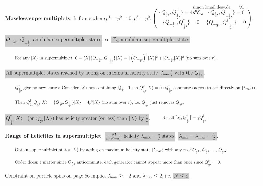
Massless supermultiplets: In frame where p1 = p2 = 0, p3 = p0,
Q12r, Q†
12s = 4p0δrs Q1
2r, Q†
− 12s = 0
Q−12r, Q†
12s = 0 Q−1
2r, Q†
− 12s = 0
.
Q−12r
, Q†− 1
2rannihilate supermultiplet states , so Zrs annihilate supermultiplet states .
For any |X〉 in supermultiplet, 0 = 〈X|Q− 12r, Q†
− 12r|X〉 = |
(Q− 1
2r
)†|X〉|2 + |Q− 1
2r|X〉|2 (no sum over r).
All supermultiplet states reached by acting on maximum helicity state |λmax〉 with the Q12r
.
Q†12r
give no new states: Consider |X〉 not containing Q 12r
. Then Q†12r|X〉 = 0 (Q†
12r
commutes across to act directly on |λmax〉).
Then Q†12rQ1
2r|X〉 = Q 1
2r, Q†
12r|X〉 = 4p0|X〉 (no sum over r), i.e. Q†
12r
just removes Q12r
.
Q†12r|X〉 (or Q1
2r|X〉) has helicity greater (or less) than |X〉 by 1
2 . Recall [J3, Q†12r
] = 12Q
†12r
.
Range of helicities in supermultiplet: N !n!(N−n)! helicity λmax − n
2 states , λmin = λmax − N2 .
Obtain supermultiplet states |X〉 by acting on maximum helicity state |λmax〉 with any n of Q 121, Q1
22, ..., Q12N
.
Order doesn’t matter since Q 12a
anticommute, each generator cannot appear more than once since Q212r
= 0.
Constraint on particle spins on page 56 implies λmin ≥ −2 and λmax ≤ 2, i.e. N ≤ 8 .

[email protected] 92SM particles probably belong to ∼ massless supermultiplets.
Superpartners (masses ∼M) of SM particles (∼ m) not seen, i.e. M ≫ m, so SUSY is broken, at energy < mSUSY.
SUSY restored at mSUSY ∴ mSUSY ≫M −m ∼M (superpartner has same mass) ∴ supermultiplets ∼ massless.
Most likely scenario is simple SUSY: quark, lepton (spin 12) superpartners are scalars (0): squarks, sleptons.
Higgs (0), gauge bosons (1), graviton (2) superpartners fermionic: Higgsino + gauginos (12), gravitino (3
2).
No alternatives: In simple SUSY, SM gauge bosons cannot be superpartners of SM fermions.
SM fermions, gauge bosons in different representations (recall simple SUSY and SM SU(3)×SU(2) commute from page 89).
Quarks, leptons cannot be in same supermultiplet as any beyond-SM vector (gauge) bosons.
Gauge bosons are in adjoint representation of a group. If e.g. helicity +12 fermion, +1 gauge boson in same supermultiplet,
fermion in adjoint = real representation. But SM is chiral, i.e. helicity +12 fermions belong to complex representations.
Superpartners of gauge bosons must be helicity ±12, not ±3
2, fermions.
Helicity ±32 particle couples only to Qa (principle of equivalence on page 56: ±2 only couples to P µ).
Extended SUSY probably cannot be realised in nature.
In extended SUSY, helicity ±12 fermions either in same supermultiplet as gauge bosons (N ≥ 3), or each other (N = 2).

[email protected] 93Massive supermultiplets: For particles with masses M ≫ mSUSY, e.g. heavy gauge bosons in SU(5).
In frame where p1 = p2 = p3 = 0, p0 = M ,
Q12r, Q†
12s = 2Mδrs Q1
2r, Q†
− 12s = 0
Q−12r, Q†
12s = 0 Q−1
2r, Q†
− 12s = 2Mδrs
,
so Q12r
, Q†− 1
2r(or Q−1
2r, Q†
12r
) lower (or raise) spin 3 component by 12.
aA(a,r) = 1√2MQar are fermionic annihilation / creation operators: aA, a†B = δAB, aA, aB = a†A, a
†B = 0.
Define Clifford “vacuum” |Ω〉: aA|Ω〉 = 0. |Ω〉 has given spin j, range of spin 3 is −j ≤ σ ≤ j.
Supermultiplet is all states a†A1. . . a†An|Ω〉, spins ranging from Max(j − N
2 , 0), . . ., j + N2 .
Simple SUSY: States with spin j ± 12, and 2 sets of states with spin j.
If j = 0, there are two bosonic spin 0 states and two fermionic states of spin 12 (i.e. spin 3 is ±1
2).
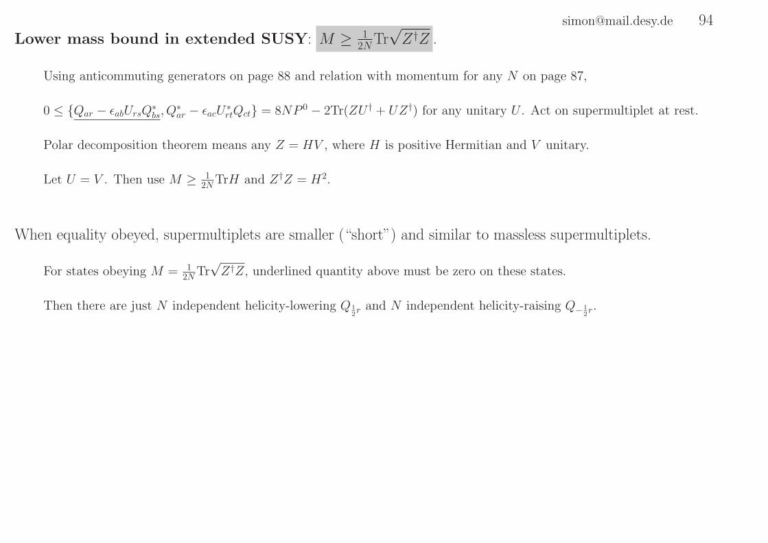
[email protected] 94Lower mass bound in extended SUSY: M ≥ 1
2NTr√Z†Z .
Using anticommuting generators on page 88 and relation with momentum for any N on page 87,
0 ≤ Qar − ǫabUrsQ∗bs, Q
∗ar − ǫacU
∗rtQct = 8NP 0 − 2Tr(ZU † + UZ†) for any unitary U . Act on supermultiplet at rest.
Polar decomposition theorem means any Z = HV , where H is positive Hermitian and V unitary.
Let U = V . Then use M ≥ 12NTrH and Z†Z = H2.
When equality obeyed, supermultiplets are smaller (“short”) and similar to massless supermultiplets.
For states obeying M = 12NTr
√Z†Z, underlined quantity above must be zero on these states.
Then there are just N independent helicity-lowering Q 12r
and N independent helicity-raising Q− 12r
.

[email protected] 953.3.1 Field supermultiplets (the left-chiral supermultiplet)
Simplest case: N = 1, scalar φ(x) obeying [Q†b, φ(x)] = 0 : Write [Qa, φ(x)] = −Iζa(x) , which is a
(12, 0)
field.
Q†a, ζb(x) = 2σµba∂µφ(x) . Thus [Q, φ] ∼ ζ and Q†, ζ ∼ φ, i.e. φ and ζ are each others’ superpartners.
Q†a,−Iζb = Q†
a, [Qb, φ] = [Q†a, Qb, φ] = 2σµba[Pµ, φ]. Poincare transformation for fields on page 25: [Pµ, φ] = I∂µφ.
Qa, ζb(x) = 2IǫabF (x) .
Qa,−Iζb = Qa, [Qb, φ] = −Qb, [Qa, φ] = −Qb, Iζa ∝ ǫab. F is (0, 0) in(
12 , 0)×(
12 , 0)
= (0, 0) + (1, 0).
[Qa,F (x)] = 0 . F has no superpartner, it is auxiliary field.
2Iǫab[Qc,F ] = [Qc, Qa, ζb] = −[Qa, Qc, ζb] = −2Iǫcb[Qa,F ]. For a = c 6= b, 2Iǫcb[Qc,F ] = −2Iǫcb[Qc,F ], so [Qc,F ] = 0.
[Q†a,F (x)] = −σµ ab∂µζb(x) .
2Iǫab[Q†c,F ] = [Q†
c, Qa, ζb] = [Q†c, Qa, ζb] − [Qa, Q†
c, ζb] = [2σµacPµ, ζb] − [Qa, 2σµbc∂µφ] = 2Iσµac∂µζb − 2Iσµbc∂µζa.
Then ǫdaǫab[Q†c,F ] = δdb[Q
†c,F ] = ǫdaσµac∂µζb − ǫdaσµbc∂µζa = ǫdaσµac∂µζb − σµbc∂µζ
d. Sum d = b: δdd[Q†c,F ] = 2[Q†
c,F ] = −2σµbc∂µζb.
Then [Q†a,F ] = ǫac[Q†c,F ] = −ǫacσµbcǫbdζd = −σµ adζd, using 4-vector σ matrices with raised indices on page 42.
Conjugation of everything above gives right-chiral supermulitplet.

To simplify algebra, use 4-component Majorana spinors, ψ =
(Xa
X†b
), with notation of page 43.
Majorana conjugation: ψ = ψTγ5E where E =
(ǫab 0
0 −ǫab(= ǫab)
). From ψ = ψ†β = (Xa, X†
b).
(Anti)commutation relations: Q,Q = −2IγµPµ and [Q,P µ] = 0 , where Majorana Q =
(Qa
Q†b = (ǫbcQc)†
).
Directly from relations on page 87.
Infinitesimal transformation of operator O : δO = [IαQ,O ] ,
where Grassmann spinor α =
(αaα†b
), so αQ = αaQa + α†
bQ†b . Implies δO† = [IαQ,O†] .
(δO)† = [IαQ,O]† = [IαQ,O†] = δ(O†), because, as for scalar from 2 spinors and Hermitian conjugate of scalar on page 41,
(αQ)† = (αaQa + α†bQ†b)† = (Q†
aα†a +Qbαb) = (−α†aQ†
a − αbQb) = (α†
aQ†a + αbQb) = αQ.
Product rule for δ: δ(AB) = (δA)B + AδB , where A, B can be fermionic / bosonic.
[IαQ,AB] = I(αQAB − ABαQ) = I(αQAB − AαQB + AαQB − ABαQ) = [IαQ,A]B + A[IαQ,B].
If Abelian limit on page 8 obeyed, finite transformation is O → eIαQOe−IαQ.
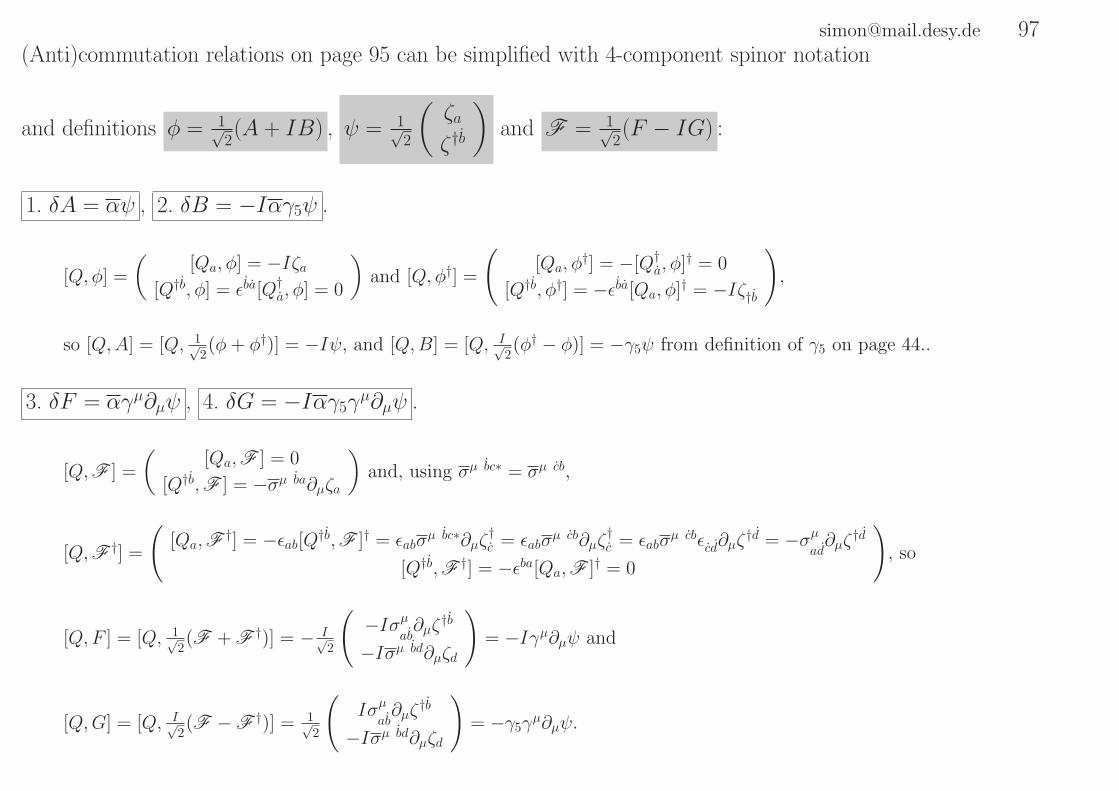
[email protected] 97(Anti)commutation relations on page 95 can be simplified with 4-component spinor notation
and definitions φ = 1√2(A + IB) , ψ = 1√
2
(ζaζ†b
)and F = 1√
2(F − IG) :
1. δA = αψ , 2. δB = −Iαγ5ψ .
[Q, φ] =
([Qa, φ] = −Iζa
[Q†b, φ] = ǫba[Q†a, φ] = 0
)and [Q, φ†] =
([Qa, φ
†] = −[Q†a, φ]† = 0
[Q†b, φ†] = −ǫba[Qa, φ]† = −Iζ†b
),
so [Q,A] = [Q, 1√2(φ+ φ†)] = −Iψ, and [Q,B] = [Q, I√
2(φ† − φ)] = −γ5ψ from definition of γ5 on page 44..
3. δF = αγµ∂µψ , 4. δG = −Iαγ5γµ∂µψ .
[Q,F ] =
([Qa,F ] = 0
[Q†b,F ] = −σµ ba∂µζa
)and, using σµ bc∗ = σµ cb,
[Q,F †] =
([Qa,F †] = −ǫab[Q†b,F ]† = ǫabσ
µ bc∗∂µζ†c = ǫabσ
µ cb∂µζ†c = ǫabσ
µ cbǫcd∂µζ†d = −σµ
ad∂µζ
†d
[Q†b,F †] = −ǫba[Qa,F ]† = 0
), so
[Q,F ] = [Q, 1√2(F + F †)] = − I√
2
(−Iσµ
ab∂µζ
†b
−Iσµ bd∂µζd
)= −Iγµ∂µψ and
[Q,G] = [Q, I√2(F − F †)] = 1√
2
(Iσµ
ab∂µζ
†b
−Iσµ bd∂µζd
)= −γ5γ
µ∂µψ.

[email protected] 985. δψ = ∂µ(A + Iγ5B)γµα + (F − Iγ5G)α .
[IαQ, ψ] = I√2
(αcQc, ζa + α†
dQ†d, ζa
αcQc, ζ†b + α†
dQ†d, ζ†b
)= I√
2
(αcQc, ζa + α†
dǫdcQ†
c, ζaαcQ†
c, ζd†ǫbd + α†dǫdcǫbaQc, ζa†
)
= I√2
(αc(2IǫcaF ) + α†
dǫdc(2σµac∂µφ)
ǫcaαa(2σµ
cd∂µφ
†)ǫbd − α†dǫdcǫba(2IǫcaF †)
)
= I√
2
( −αa(IF ) − α†c(σµac∂µφ)
−αa(σµ ba∂µφ†) − α†b(IF †)
)=
(αa(F − IG) − Iσµacα
†c∂µ(A+ IB)
α†b(F + IG) − Iσµ baαa∂µ(A− IB)
).
For L = −12∂µA∂
µA− 12∂µB∂
µB − 12ψγ
µ∂µψ + 12(F
2 +G2) +m(FA +GB − 12ψψ)
+g[F (A2 +B2) + 2GAB − ψ(A + Iγ5B)ψ] , above transformations 1 — 5 leave action A =∫d4xL invariant .
For example, for m = g = 0, δL = −∂µδA∂µA− ∂µδB∂µB − (δψ)γµ∂µψ + FδF +GδG.
We have replaced −12ψγ
µ∂µδψ → −12(δψ)γµ∂µψ, since difference with analogous term in hermitian conjugate (h.c.) of L
(must be added to make L real) is total derivative ∂µf which doesn’t contribute to A :
(Xγµ∂µZ)† = (X†βγµ∂µZ)† = (∂µZ†)㵆β†X = −(∂µZ
†)βγµX = −(∂µZ)γµX = Zγµ∂µX − ∂µ(ZγµX).
No derivatives of F , G (or F ) appear, so they are auxiliary fields,
i.e. can be expressed in terms of the other supermultiplet fields by solving equations of motion ∂L∂F = ∂L
∂G = 0.

[email protected] 99Problems 2
1: Derive the equal time anticommutation relations [ψl(x, t), ψ†l′(y, t)]+ = δll′δ
(3)(x − y) for a(
12 , 0)
+(0, 1
2
)field ψ(x) =∫
d3p(2π)3
[eIp·xuσ(p)aσ(p) + e−Ip·xvσ(p)ac†σ (p)
]where u and v obey the projection operator properties ul σ(p)ul′ σ(p) =
12p0 (−Iγµpµ +m)ll′ and vl σ(p)vl′ σ(p) = 1
2p0 (−Iγµpµ −m)ll′.
2: Show that the canonically conjugate momenta to the(
12 , 0)
+(0, 1
2
)field ψ(x) for the Lagrangian density LDirac =
−ψ (γµ∂µ +m)ψ is consistent with the equal time anticommutation relations [ψl(x, t), ψ†l′(y, t)]+ = δll′δ
(3)(x − y).
3: Under a local gauge transformation of a group G, the field strength Fµν = F iµνti transforms as Fµν → UFµνU
†, whereU and ti are respectively any element of G and the generators of G in any representation. By considering infinitessimaltransformations, show that this implies that Fµν transforms in the adjoint representation of G, i.e. F i → UijF
j, wherethe generators of Uij are tkji = ICkij.
4: How must the right-handed neutrino field νeR transform under the SM group in order for the Lagrangian term proportional
to EK
a (ǫφH)†aνeR to be invariant?
5: Suppose that there exists a two-component fermionic additive symmetry generator Qa which transforms in the(
12 , 0)
representation. Using the Coleman-Mandula theorem, show that Qa, Q†b = 2σµ
abPµ. What does this tell you about any
particle? (Note that, as an additive symmetry generator, Q = Qσρa†σaρ + Rσρa
†ρaσ, where σ sums over bosonic particles,
ρ over fermionic particles.)
6: For more than one spinor of such generators Qar distinguished by the label r, show that Qar, Q†bs = 2δrsσ
µ
abPµ.
7: How many different states are there in a massless supermultiplet for a given N? (Hint: working in a frame for which theparticles of a massless supermultiplet have a momentum proportional to p = (0, 0, 1, 1), show that the Q 1
2r, r = 1, . . . , N ,
are the only generators that convert the maximum helicity state |λmax〉 in this supermultiplet into any other state in thissupermultiplet, because the other fermionic generators either annihilate |λmax〉 or just remove any Q 1
2rgenerator.)
8: Starting with a field φ(x), the generators Qa and the constraint [Q†b, φ(x)] = 0, determine all the other fields in the same
supermulitplet as φ(x).
9: The adjoint of a(
12 , 0)
+(0, 1
2
)spinor ψ is defined as ψ = ψ†β. If ψ is a Majorana spinor, show that ψ = ψTγ5E. (Hint:
Write ψT =(Xa, X
†b = (ǫbcXc)†).)
10: Defining Q =(Qa, Q
†b), show that the anticommutation relations above read Q,Q = −2IγµPµ.

[email protected] 1003.4 Grassman variables
N independent Grassman variables θα are defined to obey θα, θβ = 0.
Thus θ2α = 0 (no sum), so for e.g. N = 3, any function f(θ) has the Grassman variable expansion
f(θ) = A +Bθ1 + Cθ2 +Dθ3 + Eθ1θ2 + Fθ2θ3 +Gθ3θ1 +Hθ1θ2θ3.
Define (no sums, β 6= α) ∂∂θαθα = 1, ∂
∂θαθβ = 0, ∂
∂θαθαθβ = θβ and ∂
∂θαθβθα = −θβ.
Note (β can be equal to α now) that
∂∂θα, ∂∂θβ
= 0 and
∂∂θα, θβ
= δαβ .
By anticommuting Grassman variables θα, θβ to the left, all terms in the Grassman variable expansion of any function f
will be of the form g, θαg, θβg and θαθβg, where g is independent of θα, θβ but can depend on the other θγ.
Then show
[∂∂θα
∂∂θβ
+ ∂∂θβ
∂∂θα
][
∂∂θαθβ + θβ
∂∂θα
](β 6= α)
g = 0θαg = 0θβg = 0θαθβg = 0
and (no sum, β 6= α)
[∂∂θαθα + θα
∂∂θα
]
g = g
θαg = θαg
θβg = θβgθαθβg = θαθβg
.
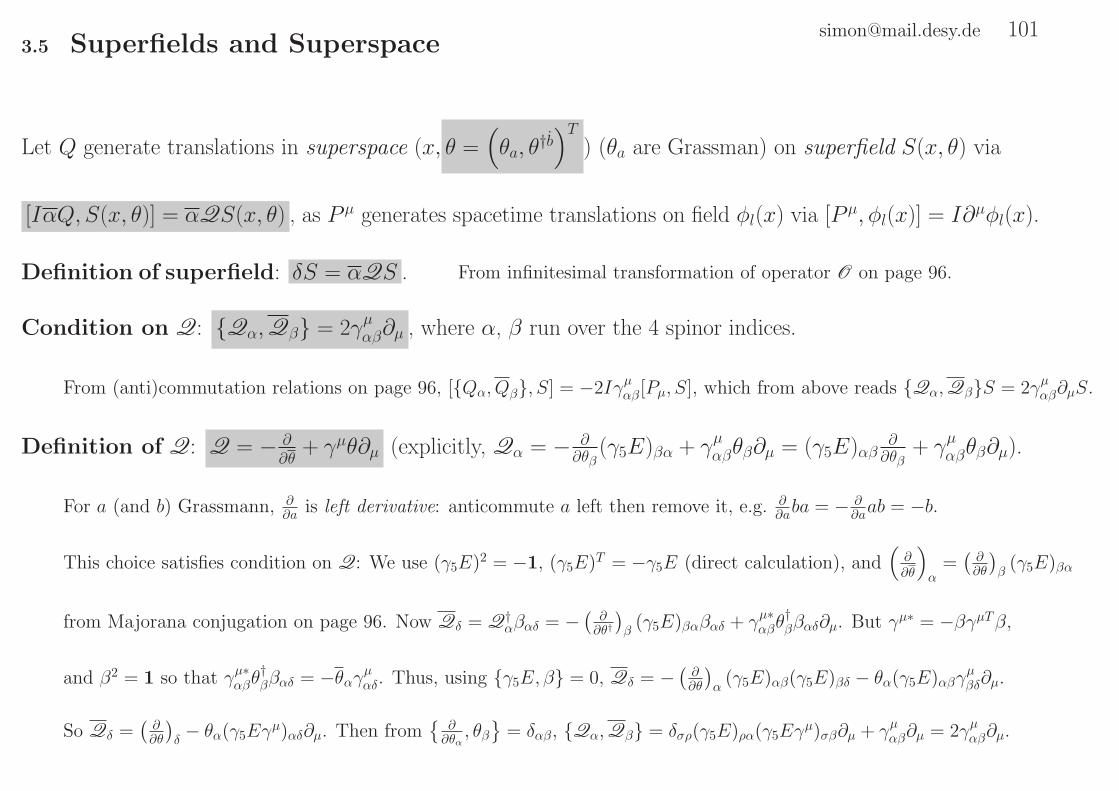
[email protected] 1013.5 Superfields and Superspace
Let Q generate translations in superspace (x, θ =(θa, θ
†b)T
) (θa are Grassman) on superfield S(x, θ) via
[IαQ, S(x, θ)] = αQS(x, θ) , as P µ generates spacetime translations on field φl(x) via [P µ, φl(x)] = I∂µφl(x).
Definition of superfield: δS = αQS . From infinitesimal transformation of operator O on page 96.
Condition on Q: Qα,Qβ = 2γµαβ∂µ , where α, β run over the 4 spinor indices.
From (anti)commutation relations on page 96, [Qα, Qβ, S] = −2Iγµαβ[Pµ, S], which from above reads Qα,QβS = 2γµαβ∂µS.
Definition of Q: Q = − ∂∂θ
+ γµθ∂µ (explicitly, Qα = − ∂∂θβ
(γ5E)βα + γµαβθβ∂µ = (γ5E)αβ∂∂θβ
+ γµαβθβ∂µ).
For a (and b) Grassmann, ∂∂a is left derivative: anticommute a left then remove it, e.g. ∂
∂aba = − ∂∂aab = −b.
This choice satisfies condition on Q: We use (γ5E)2 = −1, (γ5E)T = −γ5E (direct calculation), and(∂∂θ
)α
=(∂∂θ
)β(γ5E)βα
from Majorana conjugation on page 96. Now Qδ = Q†αβαδ = −
(∂∂θ†
)β(γ5E)βαβαδ + γµ∗αβθ
†ββαδ∂µ. But γµ∗ = −βγµTβ,
and β2 = 1 so that γµ∗αβθ†ββαδ = −θαγµαδ. Thus, using γ5E, β = 0, Qδ = −
(∂∂θ
)α(γ5E)αβ(γ5E)βδ − θα(γ5E)αβγ
µβδ∂µ.
So Qδ =(∂∂θ
)δ− θα(γ5Eγ
µ)αδ∂µ. Then from
∂∂θα, θβ
= δαβ, Qα,Qβ = δσρ(γ5E)ρα(γ5Eγµ)σβ∂µ + γµαβ∂µ = 2γµαβ∂µ.

[email protected] 102Superfields from superfields I: S = S1 + S2 , S = S1S2 , etc. are superfields when S1, S2 are superfields.
1st case clearly obeys SUSY transformation using Q above.
2nd case: From product rule for δ on page 96, δS1S2 = (δS1)S2 + S1δS2 = (αQS1)S2 + S1αQS2 = αQ(S1S2).
Superfields from superfields II: S ′ = DβS , S ′ = DβS ,
where superderivative D = − ∂∂θ
− γµθ∂µ obeys Dβ,Qγ = Dβ,Qγ = 0 .
First case: δS ′ = δDβS = [IαQ,DβS] = Dβ[IαQ, S] since αQ is a commuting object. Then δS ′ = DβαγQγS = −αγDβQγS
since αγ, Dβ anticommute. Then δS ′ = αγQγDβS = αQS ′. To show e.g. Dβ,Qγ = 0,
first obtain Dβ,Qγ =(γµαγθγ,(∂∂θ
)δ
(γ5E)δβ − α ↔ β
)∂µf and use (γµγ5E)T = γµγ5E.
Summary: Function of superfields and their superderivatives is a superfield.
R quantum number assignments for superspace: θL/R has R quantum number R = ±1 .
Recall definition of R-symmetry on page 88: Qa → eIRLφQa and Q†a → eIRRφQ†
a, where R = RL/R = ±1.
Assignments for superspace follow from definition of superfield (i.e. [Q,S(x, θ)] = −IQS(x, θ)) and definition of Q on page 101.
Note θR ∼ θ∗L.

[email protected] 103From now on, write e.g. Aµγ
µ = /A.
General form of superfield: S(x, θ) = C(x) − I [θγ5]ω(x) − I2
[θγ5θ
]M(x) − 1
2[θθ]N(x) + I2 [θγ5γµθ]V
µ(x)
−I [(θγ5θ)θ](λ(x) + 1
2/∂ω(x))− 1
4[θγ5θ]2(D(x) + 1
2∂2C(x)
),
4 (Pseudo)scalar fields: C, M , N , D, 2 Spinor fields: ω, λ, 1 Vector field: V µ
(i.e. 8 bosonic and 8 fermionic degrees of freedom).
This is most general Taylor series in θT = (θ1, θ2, θ3, θ4), or θ = θTγ5E = (−θ2, θ1, θ4,−θ3), in manifestly Lorentz invariant form:
2nd term −Iθγ5ω(x) most general quantity linear in θα.
Next 3 bilinears in θα is expansion for any bilinear B = B12θ1θ2 +B13θ1θ3 +B14θ1θ4 +B23θ2θ3 +B24θ2θ4 +B34θ3θ4:
θγ5(1Iγ0 or 1
Iγ3)θ = 2θ2θ3 ± 2θ4θ1, θγ5(1Iγ1 or 1
Iγ2)θ = 2θ2θ4 ± 2θ3θ1 (gamma matrices on page 44), θ(1 or γ5)θ = 2θ1θ2 ± 2θ4θ3.
6th term has all 4 possible cubics in θα: (θγ5θ)θ = 2(θ4θ3θ2,−θ4θ3θ1, θ1θ2θ4,−θ1θ2θ3). Last term ∝ [θγ5θ]2 = 8θ1θ2θ3θ4.
Any higher products of θα vanish, since θ2α = 0 (no sum). E.g. θ1θ2θ3θ4θ3 = −θ1θ2θ
23θ4 = 0.

[email protected] 104Superfield transformation: δS = Iαγ5ω + θ(−/∂C + Iγ5M +N − Iγ5 /V )α + I
2 [θγ5θ]α(λ + /∂ω)
−I2 [θθ]αγ5(λ + /∂ω) + I
2 [θγ5γµθ]αγµλ + I
2 [θγ5γνθ]α∂νω
+12[(θγ5θ)θ]
(I/∂M − γ5/∂N − I∂µ /V γµ + γ5(D + 1
2∂2C))α− I
4 [θγ5θ]2αγ5(/∂λ + 1
2∂2ω) .
From definition of superfield and of Q, on page 101, i.e. δS = α(− ∂∂θ
+ γµθ∂µ
)S.
Note for M = 1, M = γ5γµ and M = γ5, we have ∂∂θ
(θMθ) = 2Mθ. See also Weinberg III (hardback), page 63.
Component field transformations: δC = I(αγ5ω) , δω = (−Iγ5/∂C −M + Iγ5N + /V )α ,
δM = −α(λ + /∂ω) , δN = Iαγ5(λ + /∂ω) , δVµ = α(γµλ + ∂µω) ,
δλ = (12[∂µ /V, γµ] + Iγ5D)α and δD = Iαγ5/∂λ .
Compare superfield transformation above with general form of superfield on page 103.
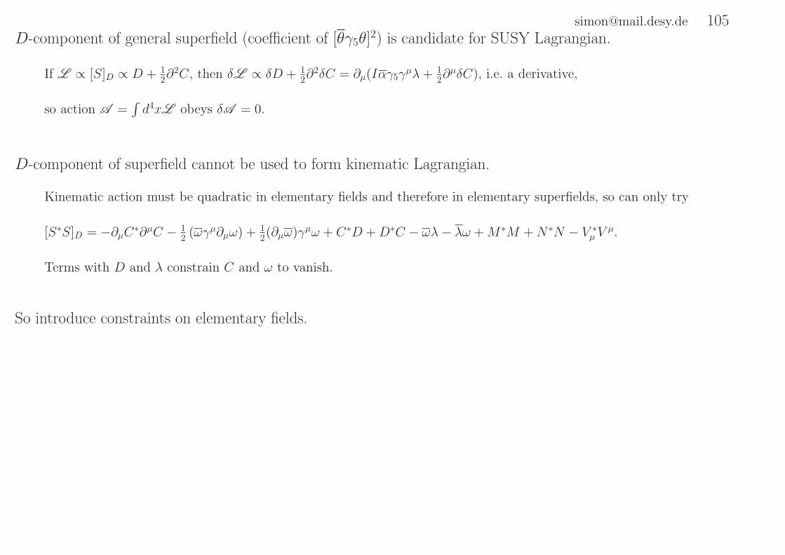
[email protected] 105D-component of general superfield (coefficient of [θγ5θ]
2) is candidate for SUSY Lagrangian.
If L ∝ [S]D ∝ D + 12∂
2C, then δL ∝ δD + 12∂
2δC = ∂µ(Iαγ5γµλ+ 1
2∂µδC), i.e. a derivative,
so action A =∫d4xL obeys δA = 0.
D-component of superfield cannot be used to form kinematic Lagrangian.
Kinematic action must be quadratic in elementary fields and therefore in elementary superfields, so can only try
[S∗S]D = −∂µC∗∂µC − 12 (ωγµ∂µω) + 1
2(∂µω)γµω + C∗D +D∗C − ωλ− λω +M ∗M +N ∗N − V ∗µ V
µ.
Terms with D and λ constrain C and ω to vanish.
So introduce constraints on elementary fields.

[email protected] 1063.5.1 Chiral superfield
Definition of chiral superfield X(x, θ): λ = D = 0 , Vµ = ∂µB , B is scalar field with δB = αω .
This is superfield because these conditions are preserved by SUSY transformations: δD = Iαγ5/∂λ = 0,
and δλ = (12 [∂µ /V, γµ] + Iγ5D)α = 1
2 [∂µ /V, γµ]α = 0 because Vµ = ∂µB: [∂µ /V, γµ] = ∂µ∂νB[γν, γµ] = 0.
Finally, δV µ = α(γµλ+ ∂µω) = ∂µαω, i.e. δB = αω, i.e. Vµ = ∂µB condition is preserved.
Chiral superfield decomposition: X(x, θ) = 1√2[Φ+(x, θ) + Φ−(x, θ)] with left / right-chiral superfields
Φ±(x, θ) = φ±(x) −√
2 θψL/R(x) + [θPL/Rθ]F±(x) ± 12[θγ5γµθ]∂
µφ±(x) ∓ 1√2(θγ5θ)θ/∂ψL/R(x) − 1
8[θγ5θ]2∂2φ±(x) ,
with ψL/R = PL/Rψ , φ± = 1√2(A± IB) , F± = 1√
2(F ∓ IG) .
To make contact with notation on page 97, write C = A, ω = −Iγ5ψ, M = G, N = −F , for later convenience
in general form of superfield on page 103, so X = A− θψ + 12θθF − I
2θγ5θG+ I2θγ5γµθ∂
µB + 12(θγ5θ)θγ5/∂ψ − 1
8 [θγ5θ]2∂2A.
Φ± is obtained from Φ± = A′ − θψ′ + 12θθF
′ − I2θγ5θG
′ + I2θγ5γµθ∂
µB′ + 12(θγ5θ)θγ5/∂ψ
′ − 18 [θγ5θ]
2∂2A′ with F ′ = ±G′,
B′ = ∓IA′, ψ′ =√
2ψL/R, i.e. by taking N = ±IM , B = ∓IC, ω = ± left/right-handed spinor in general form of superfield
on page 103, which is preserved under component field transformations on page 104.

[email protected] 107Left / right transformation: δψL/R =
√2(∂µφ±γµPR/L + F±PL/R)α , δF± =
√2 α/∂ψL/R , δφ± =
√2 αψL/R .
So left-chiral supermultiplet here = that on page 95 (ζa = ψL, φ = φ+, F = F+), right-chiral by conjugation.
Compact form: Φ±(x, θ) = φ±(x±) ∓√
2 θTL/RE ψL/R(x±) ± θTL/REθL/R F±(x±) ,
where θL/R = PL/Rθ , xµ± = xµ ± θTREγµθL .
Recall ψT = 1√2
(ζa, ζ
†b)
from page 97. This is left / right-chiral superfield on page 106, by Taylor expansion in θTREγµθL:
Make use of θT = −θγ5E (Majorana conjugation on page 96) and E2 = (γ5E)2 = −1. Also xµ± = xµ ± 12θγ5γ
µθ
(see alternative form for x± on page 108). Firstly, rewrite as Φ±(x, θ) = φ±(x±) −√
2 θPL/Rψ(x±) + θPL/RθF±(x±),
because θTL/REψL/R = −θγ5E12(1 ± γ5)E
12(1 ± γ5)ψ = −θ 1
2(−γ5 ∓ 1)12(1 ± γ5)ψ = ±θPL/Rψ.
1st term in underlined equation above: φ±(x±) = φ±(x) ± 12(θγ5γµθ)∂
µφ±(x) − 12(
12θγ5γ
µθ)(12θγ5γ
νθ)∂µ∂νφ±(x)
= φ±(x) ± 12(θγ5γµθ)∂
µφ±(x) − 12(
12θγ5θ)
2 12γµ, γν∂µ∂νφ±(x), then use 1
2γµ, γν = gµν.
2nd term: −√
2 θPL/Rψ(x±) = −√
2 θPL/Rψ(x) ∓ 1√2(θγ5γ
µθ)θ∂µPL/Rψ(x) = −√
2 θPL/Rψ(x) ∓ 1√2(θγ5θ)θγ
µ∂µPL/Rψ(x).
3rd term: θPL/RθF±(x±) = θPL/RθF±(x) ± 12θγ5γ
µθθPL/Rθ∂µF±(x) = θPL/RθF±(x) + [(θTREγµθL)(θ
TL/REθL/R)∂µF±(x)],
term in square brackets vanishes due to 3 occurences of “2-component” θL/R.

[email protected] 108Alternative form for x±: xµ± = xµ ± 1
2θγ5γµθ .
Recall xµ± = xµ ± θTREγµθL. Now 1
2θγ5γµθ = 1
2θTγ5Eγ5γ
µθ = −12θ
Tγ5Eγµγ5θ using γµ, γ5 = 0. But γ5 = PL − PR,
so 12θγ5γ
µθ = 12θ
T (PL − PR)Eγµ(PR − PL)θ = 12θ
TPLEγµPRθ + 1
2θTPREγ
µPLθ − 12θ
TPLEγµPLθ − 1
2θTPREγ
µPRθ.
3rd and 4th terms zero because PL/REγµPL/R = EPL/Rγ
µPL/R = EγµPR/LPL/R = 0.
2nd term is 12θ
TPREγµPLθ = −(1
2θTPREγ
µPLθ)T = −1
2θTPL(Eγ
µ)TPRθ (− sign because components of θ anticommute).
But (Eγµ)T = −Eγµ, so 2nd term = 1st term, i.e. 12θγ5γ
µθ = θTREγµθL.
Relations between superspace directions: x∗+ = x− .
I.e. show θREγµθL = θγ5γ
µθ is “imaginary”.
x∗+ = xµ + θ†REγµ∗θ∗L. But θTR = (0, θ†b), so θ†R = (0, θb) = θLEβ, and θL = (θa, 0)T so θ∗L = (θ†a, 0)T = EβθR,
and γµ∗ = −βγµTβ. These results together with β2 = −E2 = 1, βE = Eβ and ET = −E give θ†REγµ∗θ∗L = −θREγµθL.
Alternatively, use xµ± = xµ ± 12θγ5γ
µθ and show (θγ5γµθ)† = −θγ5γ
µθ:
(θγ5γµθ)† = (θ†βγ5γ
µθ)† = −θ†γ†µγ5βθ (− sign because components of θ anticommute).
Then inserting β2 = 1 in places, (θγ5γµθ)† = −(θ†β)(βㆵβ)(βγ5β)θ = θγµγ5θ = −θγ5γ
µθ.

[email protected] 109Compact form on page 107 is most general function of x± and θL/R.
So any function of left-chiral superfields is left-chiral superfield (likewise right).
Conjugate of right-chiral superfield is left-chiral superfield. Chiral superfield decomposition, page 106: Use (θγ5)∗ = −θγ5.
Superspace “direction” of chiral superfield: D∓Φ± = 0 , where superderivative D∓ = PR/LD .
Can be used to define left / right-chiral superfield.
Follows from D∓xµ± = 0, using D∓α = ∓Eαβ
∂∂θR/L β
− (γµθL/R)α∂∂xµ . D−f(x, θ) = 0 implies f(x, θ) = f ′(x+, θL), i.e. f is left-chiral:
Any function f(x, θ) = g(x+, θR, θL) =∑
a g(a)(x+)h(a)(θR, θL), where each h(a) is all possible products
of between 1 and 4 components of θ. Using first D−,αg(a)(x+) = 0 then D−,αh(a)(θR, θL) = −Eαβ∂
∂θR βh(a)(θR, θL),
we require EαβD−,βf =∑
a g(a)(x+) ∂
∂θR αh(a)(θR, θL) = 0. Therefore if h(a) contains θR α, g
(a)(x+) = 0.
Chiral superfield from superfield: For general superfield S, D±αD±βS (i.e. DT±ED±S) is left / right-chiral.
D±γ(D±αD±βS) = 0 because the D±α anticommute and there are only 2 of them.
F -component of chiral superfield (coefficient of θPLθ) is candidate for SUSY Lagrangian.
If L ∝ [Φ±]F = F±, then δL ∝ α/∂ψL/R, i.e. a derivative, so action A =∫d4xL obeys δA = 0.

[email protected] 110Any left/right-chiral superfield Φ± can be written Φ± = D2
R/LS respectively,
where S is a general superfield and D2R/L = EαβD∓,αD∓,β.
Expand S = f1(x+, θL) + f2(x+, θL)θR1 + f3(x+, θL)θR2 + f4(x+, θL)θR1θR2.
But D−,αf(x+, θL) = 0 because D−α = −Eαβ∂
∂θR β− (γµθL)α
∂∂xµ and D−αx+ = 0.
Thus D−αS = −Eαβ∂
∂θR βS, giving D2
R/LS = −2f4(x+, θL),
where f4(x+, θL) is any function of (x+, θL), i.e. a general lef-chiral superfield.

[email protected] 1113.5.2 Supersymmetric Actions
From now on, only work with left-chiral superfields, write Φ+ = Φ, φ+ = φ, F+ = F .
Supersymmetric action from chiral superfields: A =∫d4x[f ]F +
∫d4x[f ]∗F +
∫d4x1
2[K]D ,
where f is left-chiral, K is real superfield.
Superpotential f is polynomial in left-chiral superfields.
Recall from page 109 that function of left-chiral superfields (but not complex conjugates thereof) is left-chiral superfield.
Superderivatives (and therefore derivatives) of left-chiral superfield is not left-chiral. Let S be a general superfield.
If (a term in) f contains a left-chiral superfield of form D−αD−βS (see chiral superfield from superfield on page 109),
can write f = D2Rh where h is product of S with left-chiral superfields,
since D− annihilates all left-chiral superfields after differentiating with product rule.
But D2Rh ∝ coeff. of θTREθR in h (neglecting spacetime derivatives which don’t contribute to A from now on).
Then [D2Rh]F ∝ coeff. of (θTLEθL)(θ
TREθR) = (θγ5θ)
2 in h, i.e. [h]D, so∫d4x[D2
Rh]F ∝∫d4x[h]D,
i.e. D2RS terms not necessary in f , can be included in [K]D.
Kahler potential K depends on left / right-chiral superfields but is more general.

[email protected] 112R quantum number assignments for potentials f and K: Rf = 2 , RK = 0 .
First case: Want∫d4x[f ]F to have RF = 0. From chiral superfield decomposition on page 106, term in left-chiral superfield Φ
containing F component is θPLθF = ±θTLEθLF . Since RθTLEθL= 2 and want RF = 0, must have Rf = 2.
Second case: Want∫d4x[K]D to have RD = 0. From general form of superfield on page 103,
term containing D component is ∝ [θγ5θ]2(D + 1
2∂2C). But R[θγ5θ]2
= 0, so for RD = 0 must have RK = 0.
For renormalizable theory of chiral superfields:
Superpotential f is at most cubic in left-chiral superfields Φn.
Operators O in L must have mass dimension dM(O) ≤ 4 for renormalizability. From definition of D , dM(θ) = −12 .
So dM([S]F ) = dM(S) + 1, dM([S]D) = dM(S) + 2, so operators (represented by S here) in f (K) have dM(S) ≤ 3(2).
Since dM(Φ±) = dM(φ±) = 1, f can only be cubic polynomial in Φn.
General form of Kahler potential: K(Φ,Φ∗) =∑
mn gmnΦ∗mΦn , gmn Hermitian and positive-definite.
As noted above, operators in K have mass dimensionality ≤ 2. ΦmΦn terms (or conjugates thereof) don’t appear,
since they are left-chiral so have no D term. gmn positive-definite to get correct commutation relations for fields.

[email protected] 113Kahler potential part of L : 1
2[K(Φ,Φ∗)]D = −∂µφ∗n∂µφn + F ∗nFn − 1
2ψnLγµ∂µψnL + 1
2(∂µψnR)γµψnR .
Direct calculation gives 12 [K(Φ,Φ∗)]D = gmn
[−∂µφ∗m∂µφn + F ∗
mFn − 12ψmLγ
µ∂µψnL + 12(∂µψmR)γµψnR
].
Take Φ′m = NmnΦn, g
′mn = (N †gN)mn. Since gmn Hermitian, choose unitary N to diagonalize it.
Diagonal terms positive to get positive coefficient for −∂µφ′∗n ∂µφ′n, absorb them into φ′n then drop primes.
Superpotential part of L : [f(Φ)]F = −12∂2f(φ)∂φn∂φm
ψnRψmL + Fn∂f(φ)∂φn
. Similar for f ∗.
Use compact form on page 107 to write f(Φ) = f(φ+(x+) −√
2 θTLE ψL(x+) + θTLEθL F+(x+)).
Taylor expand this in −√
2 θTLE ψL(x+) + θTLEθL F+(x+). Note e.g. θLαθLβ = EαβθL1θL2 for α, β ≤ 1, 2, but = 0 otherwise.
Replace x+ with x because θTREγµθL gives zero when acting on expression with 2 θL factors.
L from chiral superfields: L = −∂µφ∗n∂µφn − 12ψnLγ
µ∂µψnL + 12(∂µψnR)γµψnR
−12∂2f(φ)∂φn∂φm
ψnRψmL − 12
(∂2f(φ)∂φn∂φm
)∗(ψnRψmL)∗ − V (φ) ,
where Fn = −(∂f(φ)∂φn
)∗and scalar field potential V (φ) =
∑n
∣∣∣∣∂f(φ)∂φn
∣∣∣∣2
.
Sum Kahler potential and superpotential parts (and conjugate) of L above, use field equations to get Fn = −(∂f(φ)∂φn
)∗.

Zeroth order φn0 = 〈0|φn|0〉 at minimum of V (φ). If ∂f(φ)∂φn
∣∣∣∣φ=φ0
= 0 possible, V (φ0) = 0 and SUSY unbroken.
Tree-level expansion of V : V (φ) = (M †M )mn∆φ†m∆φn ,
where ∆φn = φn − φn0 , bosonic mass matrix Mmn = ∂2f∂φm∂φn
∣∣φ=φ0
.
V =∑
n
∣∣∣∣∂f∂φn
∣∣∣∣2
≃∑n
∣∣∣∣∂2f
∂φm∂φn
∣∣φ=φ0
∆φm
∣∣∣∣2
= ∆φ†m(M †M )mn∆φn.
Matrix M is complex symmetric, so can be diagonalised by unitary matrix such that diagonal terms are real and positive.
From L from chiral superfields on page 113, fermionic mass term is −12MmnψnRψmL,
so fermions and bosons have same mass, as required in SUSY.
Free Lagrangian density: L0 =∑
n
[− ∂µ∆φ
∗n∂
µ∆φn −m2n∆φ
∗n∆φn
−12ψnLγ
µ∂µψnL + 12(∂µψnR)γµψnR − 1
2mnψnRψnL − 12mn(ψnRψnL)∗
].
L0 = −∂µ∆φ∗n∂µ∆φn − (M †M )mn∆φ∗m∆φn − 1
2ψnLγµ∂µψnL + 1
2(∂µψnR)γµψnR − 12MmnψnRψmL − 1
2M∗mn(ψnRψmL)
∗
from L from chiral superfields on page 113 and tree-level expansion of V above, then diagonalize M .

[email protected] 115Problems 3
1: By working in the chiral representation, show that ET = −E, (γ5E)2 = −1, (γ5E)T = −γ5E, γµ∗ = −βγµTβ, β2 = 1,γ5E, β = 0, [E, β] = 0 and (Eγµ)T = −Eγµ.
2: Show that (ψT) = −ψγ5E and γµψ = −ψγµ, where ψ is a Majorana spinor.
3: Using Qα = (γ5E)αβ∂∂θβ
+ γµαβθβ∂µ and Qδ =(∂∂θ
)δ− θα(γ5Eγ
µ)αδ∂µ, show that Qα,Qβ = 2γµαβ∂µ.
4: Show that Dβ,Qγ = 0, where Dα = (γ5E)αβ∂∂θβ
− γµαβθβ∂µ.
5: Show that the result obtained by setting λ = D = 0 and Vµ = ∂µB, where B is scalar field, in a superfield is anothersuperfield, called the chiral superfield. (Hint: show that these constraints are preserved under SUSY transformations.)
6: Show that the chiral superfield is the sum of two chiral superfields, called left- and right-handed chiral superfieldsrespectively, for which N = ±IM , B = ∓IC, ω = ± left/right-handed spinor. (Hint: show that these constraints arepreserved under SUSY transformations. Be careful not to confuse the component fields N , M , . . . of the three differentsuperfields.)
7: Show that D∓Φ± = 0, where D∓α = ∓Eαβ∂
∂θR/L β− (γµθL/R)α
∂∂xµ and xµ± = xµ ± θTREγ
µθL.
8: Show that (θREγµθL)
∗ = θREγµθL.
9: For a general superfield S, calculate DT−ED−S and show that the result is the coefficient of θTREθR in S up to spacetime
derivatives.
10: Show that the D term of ΦΦ′ vanishes, where Φ and Φ′ are left-chiral superfields.

[email protected] 1163.6 Superspace integration
Define integration over Grassman variables θα as (no sum over α 6= β 6= γ)∫dθαθα = 1,
∫dθα = 0,
more generally e.g.∫dθβdθαθαθβθγ = θγ.
Because (θγ5θ)2 = 8θ1θ2θ3θ4, then
∫d4x[S]D = −1
2
∫d4x
∫d4θS(x, θ) .
Because θTLEθL = 2θ1θ2 in compact form on page 107, then∫d4x[Φ]F = 1
2
∫d4x
∫d2θLΦ(x, θ) .
Define δ(4)(θ′ − θ) via∫d4θ′δ(4)(θ′ − θ)f(θ′) = f(θ).
Solution is δ(4)(θ′−θ) = (θ′1−θ1)(θ′2−θ2)(θ
′3−θ3)(θ
′4−θ4) = 1
4
[(θ′L − θL)T E (θ′L − θL)
] [(θ′R − θR)T E (θ′R − θR)
].
Note e.g.∫dθ1
∂∂θ1f = 0, Try f = 1 amd f = θ1.
and∫dθ1f
∂∂θ1g =
∫dθ1
(∂∂θ1f)g. Both sides zero for (f, g) = (1, 1) and (1, θ1), both sides 1 for (θ1, θ1).

[email protected] 1173.7 Supergraphs
(Super)graphs allow for preservation of Lorentz group symmetry (and SUSY) throughout calculations.
In e.g. theory of left-chiral superfields Φ∗n(x, θ) and their complex conjugates,
VEV of time-ordered product of component fields from
VEV of time-ordered product of superfields:
〈0|TΦn1(x1, θ1),Φn2(x2, θ2) . . .
|0〉 =
∫ [∏n,x,θ dΦn(x, θ)
]eIA [Φ]Φn1(x1, θ1)Φn2(x2, θ2) . . . , where
Action from spacetime integration: A [Φ] = 12
∫d4x [Φ∗
n(x, θ)Φn(x, θ)]D + 2Re∫d4x [f(Φ)]F .

To get supergraph Feynman rules, first write A [Φ] in form A =∫d4x∫d4θ × something.
Introduce superfields Sn such that Φn = D2RSn . No loss of generality - see page 110.
Action from superspace integration: A [D2RS] =
∫d4x
∫d4θ(−1
4S∗nD
2LD
2RSn − Re[f(D2
RS, S)])
,
where f defined by f(D2RS) = D2
Rf (D2RS, S). In f , all superfields acted on by D2
R except one.
Recall D2RSn is left-chiral because DRαDRβDRγ = 0.
So Φ∗n(x, θ)Φn(x, θ) = (D2
LS∗n)D
2RSn = S∗
nD2LD
2RSn + EαβDLα((DLβS
∗n)D
2RSn + S∗
nDLβD2RSn).
Now for any superfield T , [DL/RT ]D = 0, so [Φ∗n(x, θ)Φn(x, θ)]D = [S∗
nD2LD
2RSn]D.
Because e.g. (D2RT )n = D2
R(T (D2RT )n−1) (follows from (D2
R)2 = 0) then f(D2RS) = D2
Rf(D2RS, S).
From page 111,∫d4x[DT
−ED−h]F ∝∫d4x[h]D, i.e.
∫d4x[D2
Rf(D2RS, S)]F =
∫d4x[f(D2
RS, S)]D.
So A =∫d4x
(12
[S∗nD
2LD
2RSn
]D
+ 2Re[f(D2
RS, S)]D
). Then use
∫d4x[S]D = −1
2
∫d4x
∫d4θS(x, θ) from page 116.

[email protected] 119Also we can replace
∏n,x,θ dΦn(x, θ) →
∏n,x,θ dSn(x, θ) in path-integral.
Consider lattice of N points, fields φi −→ ψi = φi+1 − φi = Cijφj. Then dNψ = det(C)dNφ = dNφ because det(C) = 1.
Thus VEV of time-ordered product of superfields on page 117 becomes
〈0|TΦn1(x1, θ1),Φn2(x2, θ2) . . .
|0〉 = D2
1RD22R . . .
∫ [∏n,x,θ dSn(x, θ)
]eIA [D2
RS]Sn1(x1, θ1)Sn2(x2, θ2) . . .
= D21RD2
2R . . . 〈0|TSn1(x1, θ1), Sn2(x2, θ2) . . .
|0〉.
Action invariant under Sn → Sn + DRXn, where Xn is any superfield.
In A [D2RS], D2
RS → D2RS + D2
RDRXn but D2RDR = 0.
Propagator for left-chiral superfields: ∆Φnm = 1
4D2RD ′2
L ∆F (x− y)δ(4)(θ − θ′)δnm .
Propagator for S is ∆Snm = 1
4∆F (x− y)δ(4)(θ − θ′)δnm + DR-terms (see page 120).
∆Snm is superpropagator for line created by superfield S∗
m(x′, θ′) and destroyed by Sn(x, θ),
and Φ∗m(x′, θ′) = D ′2
L S∗m(x′, θ′) and Φn(x, θ) = D2
RSn(x, θ), so ∆Φnm = D2
RD ′2L∆S
nm.

[email protected] 120Superpropagator: ∆S
nm = 14∆F (x− y)δ(4)(θ − θ′)δnm + DR-terms .
Propagator usually comes from quadratic terms in action. If i labels spacetime position (on lattice) as well as spin etc.,
so Aquad[φ] = −Dijφ∗iφj where D is Hermitian, then ∆ = D−1. But D not invertible if Aquad[φ] invariant under
φi → φi + ξi, i.e. Dijξj = 0. Let uν be remaining eigenvectors of D, i.e. (no sum over ν unless explicitly indicated)
Dijuνj = dνuνi, u∗νiuν′i = δνν′, u
∗νiξi = 0. In path integral Pa...b... =
∫ ∏i dφidφ
∗i e
Aquad[φ]φa . . . φ∗b . . ., transform from φi
to φ′(ν) with Jacobian J , where φi = φ′ξi +∑
ν φ′νuνi: With C = J
∫dφ′dφ′∗ and, up to terms with 1+ factors of ξ,
Pa...b... = C∫ ∏
ν dφ′νdφ
′∗ν e
−I∑ν dν |φ′ν |2 [∑
ν φ′νuνa] . . . [
∑ν φ
′νuνb]
∗ . . .+ ξ−terms =∑
pairings[−I∆ab] + ξ−terms,
where propagator ∆ab =∑
νuνau
∗νb
dν. Replacing Aquad with full gauge-invariant A , ξ-terms vanish
because φi contracted with objects Ji obeying Jiξi = 0. So, alternatively, solve Dac∆cb = Πab to get ∆ab,
where projection operator Πab =∑
ν uνau∗νb obeys Π2 = Π and Πξ = 0, because solution for ∆ab unique
up to these irrelevant ξ-terms. From action from superspace integration on page 118,
14D
2LD
2R∆S
nm(x, θ; x′, θ′) = Pδ(4)(x− x′)δ(4)(θ − θ′)δnm, where P obeys P2 = P and PDRXn = 0.
Solution for P is P = − 116
−1D2LD
2R, because D2
RD2LD
2R = −16D2
R and D2RDR = 0,
so solution for ∆Snm is ∆S
nm = 14∆F (x− y)δ(4)(θ − θ′)δnm + DR-terms.

[email protected] 121Generating functional: Z[J,A ] =
∫ ∏x,l dφl(x)eIA [φ]+I
∫d4xφl(x)Jl(x) . Contains all S-matrix elements.
From page 61,〈0, out|T
φlA(xA),φlB (xB),...
|0, in〉
〈0, out|0, in〉 = 1Z[J,A ]
(−I δ
δJlA(xA)
)(−I δ
δJlB (xA)
). . . Z[J,A ]
∣∣∣∣J=0
.
Z[J,A ] = tree-level part of Z[J,Γ], where
Quantum effective action: Γ[φ] = −∫d4xφl(x)Jφl(x) − I lnZ[Jφ,A ] , Jφ is solution of φl = δ(−I lnZ[J,A ])
δJl(x)
∣∣∣∣J=Jφ
.
Define Z[J,Γ, g] =∫ ∏
x,l dφl(x)eg−1[IΓ[φ]+I
∫d4xφl(x)Jl(x)], i.e. Z[J,Γ, 1] = Z[J,Γ]. Propagator for Z[J,Γ, g] is ∝ g,
because it is inverse of coefficient of term in g−1Γ[φ] which is quadratic in φl. Each vertex is ∝ g−1.
So for L = number of loops, Z[J,Γ, g] =∑∞
L=0 gL−1Z(L)[J,Γ]. Now take g → 0, so integration in Z[J,Γ, g] is dominated
by φ-configurations that give stationary phase, i.e. Z[J,Γ, g] ∝ eg−1[IΓ[φJ ]+I
∫d4xφJl(x)Jl(x)] where φJ such that
δδφl(y)
[IΓ[φ] + I
∫d4xφl(x)Jl(x)
]φ=φJ
= 0, or δδφl(x)
Γ[φ]
∣∣∣∣φ=φJ
= −Jl(x). Thus JφJ = J because, from definition of Γ[φ] and Jφ,
δδφl(x)
Γ[φ] = −∫d4yφk(y)
δJφk(y)δφl(x)
− Jφl(x) +∫d4y δ(−I lnZ[J ])
δJk(y)
∣∣∣∣J=Jφ
δJφk(y)δφl(x)
= Jφl(x). Proportionality constant in underlined equation
begins at O(g0) so, taking logs, coefficient of g−1 is −I lnZ(0)[J,Γ] = Γ[φJ ] +∫d4xφJl(x)Jl(x) = −I lnZ[JφJ ,A ] = −I lnZ[J,A ].
Coefficients of products of fields in Γ[φ] from corresponding connected 1 particle irreducible (1PI) graphs.

[email protected] 122Γ[S, S∗] is local in fermionic coordinates.
Each incoming (outgoing) external line is attached to vertex labelled (x, θ), gives a factor Sn(x, θ) (S∗n(x, θ)).
Each vertex gives factor equal to coefficient of corresponding product of fields in f(D2RS, S).
Each propagator from vertex (x, θ) to vertex (x′, θ′) gives −I4δ
(4)(θ − θ′)∆F (x− x′).
Recall from page 118 that in f all superfields acted on by D2R except one.
So a D2R (D2
L) acts on all lines but one that come into (go out of) a vertex.
But Γ[S, S∗] obtained by restricting to 1PI graphs and integrating over all xs and θs.
So use integration by parts to move all D2R (D2
L) on propagators to external line factors Sn(x, θ) (S∗n(x, θ)).
Integrate out all δ(4)(θ − θ′) so that Γ[S, S∗] is integral over single 4-D θ.
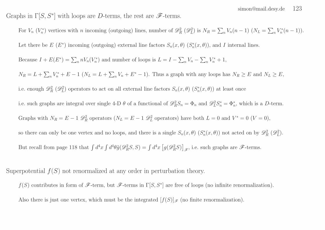
[email protected] 123Graphs in Γ[S, S∗] with loops are D-terms, the rest are F -terms.
For Vn (V ∗n ) vertices with n incoming (outgoing) lines, number of D2
R (D2L) is NR =
∑n Vn(n− 1) (NL =
∑n V
∗n (n− 1)).
Let there be E (E∗) incoming (outgoing) external line factors Sn(x, θ) (S∗n(x, θ)), and I internal lines.
Because I + E(E∗) =∑
n nVn(V∗n ) and number of loops is L = I −
∑n Vn −
∑n V
∗n + 1,
NR = L+∑
n V∗n + E − 1 (NL = L+
∑n Vn + E∗ − 1). Thus a graph with any loops has NR ≥ E and NL ≥ E,
i.e. enough D2R (D2
L) operators to act on all external line factors Sn(x, θ) (S∗n(x, θ)) at least once
i.e. such graphs are integral over single 4-D θ of a functional of D2RSn = Φn and D2
LS∗n = Φ∗
n, which is a D-term.
Graphs with NR = E − 1 D2R operators (NL = E − 1 D2
L operators) have both L = 0 and V ∗ = 0 (V = 0),
so there can only be one vertex and no loops, and there is a single Sn(x, θ) (S∗n(x, θ)) not acted on by D2
R (D2L).
But recall from page 118 that∫d4x
∫d4θg(D2
RS, S) =∫d4x
[g(D2
RS)]F
, i.e. such graphs are F -terms.
Superpotential f(S) not renormalized at any order in perturbation theory.
f(S) contributes in form of F -term, but F -terms in Γ[S, S∗] are free of loops (no infinite renormalization).
Also there is just one vertex, which must be the integrated [f(S)]F (no finite renormalization).

[email protected] 1243.8 SUSY current
SUSY current: Sµ = Jµ +Kµ (4-vector of Majorana spinors), where Kµ appears in δL = α∂µKµ ,
J is the Noether current in explicit result for Noether current when L is invariant on page 59: −αJµ = ∂RL∂(∂µχl)
δχl .
But L is bot invariant under SUSY, so add Kµ to definition of SUSY current. Then
Conservation of SUSY current: ∂µSµ = 0 .
(Following argument is general.) From definition of Jµ above, α∂µJµ = −
(∂µ
∂RL∂(∂µχl)
)δχl − ∂RL
∂(∂µχl)δ∂µχ
l.
Using Euler-Lagrange equations on page 58, α∂µJµ = −∂RL
∂χlδχl − ∂RL
∂(∂µχl)δ∂µχ
l = −δL ,
cancels δL = α∂µKµ.

[email protected] 125Generator of SUSY transformations:
[∫d3xαS0, χl
]= Iδχl .
(Following argument is general.) Let L = L(q, q), δq = δq(q, q), canonical coordinates q are all fields χl at all spacetime points.
Recall L =∫d3xL , so δL =
∫d3xα∂µK
µ =∫d3xαdK
0
dt or ∂L∂qnδq
n + ∂L∂qnδq
n = dFdt , where F =
∫d3xαK0.
But ∂L∂qn = d
dt∂L∂qn , so underlined equation is Q = 0 where conserved charge Q = − ∂L
∂qnδqn + F .
So Q =∫d3xαS0, because − ∂L
∂qnδqn =
∫d3xαJ0 from the definition of the Noether current. Must show [Q,χl] = Iδχl:
Now [Q, qm] = −[∂L∂qn , q
m]δqn − ∂L
∂qn [δqn, qm] + [F, qm]. In 1st term, use QM result[∂L∂qn , q
m]
= −Iδmn (assuming no constraints).
For 2nd and 3rd terms consider general [f(q, q), qm]. We may write f =∑∞
k=0An1...nk(q)qn1. . . qnk . Using QM result [qn, qm] = 0,
we find [f(q, q), qm] =∑∞
k=0An1...nk(q)∑k
r=1 qn1. . . qnr−1
[qnr , qm]qnr+1. . . qnk = ∂f
∂qn[qn, qm]
(in last expression, insert [qn, qm] in correct position among q products). Then [Q, qm] = Iδqm +(∂F∂qn − ∂L
∂ql∂δql
∂qn
)[qn, qm].
But ∂F∂qn = ∂L
∂ql∂δql
∂qn : In underlined equation above, replace X, where X = δqn on LHS and X = dFdt on RHS,
with chain rule X = ql ∂X∂ql
+ ql ∂X∂ql
. Then ∂L∂qnδq
n + ql ∂L∂qn∂δqn
∂ql+ ql ∂L∂qn
∂δqn
∂ql= qn ∂F∂qn + qn ∂F∂qn .
Match coefficients of qn, which does not appear implicitly in any term.
Thus [Q, qm] = Iδqm. Taking the time derivative also gives [Q, qm] = Iδqm. Can be extended to cases with constraints.

SUSY current for chiral supermultiplet: Sµ =√
2[(/∂φn)γ
µψnR + ∂f∂φnγµψnL + (φn → φ∗n, ψnR ↔ ψnL)
].
Noether current: Jµ = 1√2[2(∂µφ∗n)ψnL + 2(∂µφn)ψnR + (/∂φn)γ
µψnR + (/∂φ∗n)γµψnL − Fnγ
µψnR − F ∗nγ
µψnL]:
Use explicit result for Noether current when L is invariant on page 59, where L from chiral superfields on page 113 is
L = −∂µφ∗n∂µφn − 12ψnLγ
µ∂µψnL + 12(∂µψnR)γµψnR + non-spacetime-derivative terms,
change in fields from left / right transformation on page 107 (excluding δF±).
Next, Kµ = 1√2γµ[−(/∂φn)ψnR − (/∂φ∗n)ψnL + F ∗
nψnL + FnψnR + 2 ∂f∂φn
ψnL + 2(∂f∂φn
)∗ψnR
]:
Recall δL = α∂µKµ from page 125. In supersymmetric action from chiral superfields on page 111,
use (from left / right transformation on page 107) δ[f ]F =√
2 α/∂[f ]ψL,
and (from component field transformations on page 104) δ[K]D = Iαγ5/∂[K]λ.

Alternative SUSY current: Sµ = Kµ + Jµ +√
23 [γµ, γν]∂ν (φnψnR + φ∗nψnL) .
Can always add ∂νAµν to Sµ (Aµν is some antisymmetric tensor of spinors), because 1. it is conserved (∂µ∂νA
µν = 0),
2. generator of SUSY transformations on page 125 unchanged because∫d3xα∂νA
0ν =∫d3xα∂iA
0i = 0.
This gives
Measure of scale invariance violation: γµSµ = −2
√2(φm
∂2f∂φn∂φm
− 2 ∂f∂φn
)ψnL + (L→ R, φ→ φ∗) .
From L from chiral superfields on page 113, Dirac equations are /∂ψmL = −(
∂2f∂φm∂φn
)∗ψnR
and same with L↔ R and φ→ φ∗. Use SUSY current for chiral supermultiplet on page 126 (= Kµ + Jµ)
and alternative SUSY current above.
because γµSµ vanishes when f is 3rd order homogeneous polynomial (f = Cmnpφmφnφp),
in which case coupling (Cmnp) is dimensionless.
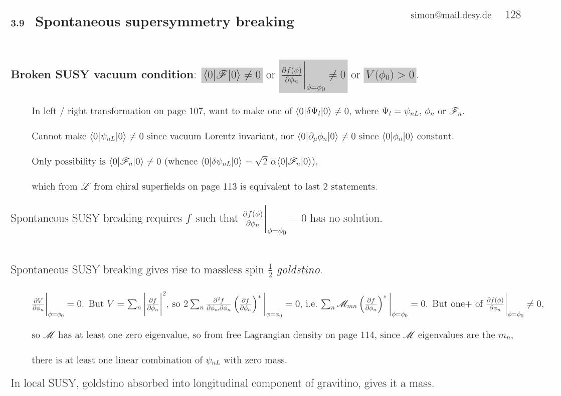
[email protected] 1283.9 Spontaneous supersymmetry breaking
Broken SUSY vacuum condition: 〈0|F |0〉 6= 0 or ∂f(φ)∂φn
∣∣∣∣φ=φ0
6= 0 or V (φ0) > 0 .
In left / right transformation on page 107, want to make one of 〈0|δΨl|0〉 6= 0, where Ψl = ψnL, φn or Fn.
Cannot make 〈0|ψnL|0〉 6= 0 since vacuum Lorentz invariant, nor 〈0|∂µφn|0〉 6= 0 since 〈0|φn|0〉 constant.
Only possibility is 〈0|Fn|0〉 6= 0 (whence 〈0|δψnL|0〉 =√
2 α〈0|Fn|0〉),
which from L from chiral superfields on page 113 is equivalent to last 2 statements.
Spontaneous SUSY breaking requires f such that ∂f(φ)∂φn
∣∣∣∣φ=φ0
= 0 has no solution.
Spontaneous SUSY breaking gives rise to massless spin 12 goldstino.
∂V∂φn
∣∣∣∣φ=φ0
= 0. But V =∑
n
∣∣∣∣∂f∂φn
∣∣∣∣2
, so 2∑
n∂2f
∂φm∂φn
(∂f∂φn
)∗ ∣∣∣∣φ=φ0
= 0, i.e.∑
n Mmn
(∂f∂φn
)∗ ∣∣∣∣φ=φ0
= 0. But one+ of ∂f(φ)∂φn
∣∣∣∣φ=φ0
6= 0,
so M has at least one zero eigenvalue, so from free Lagrangian density on page 114, since M eigenvalues are the mn,
there is at least one linear combination of ψnL with zero mass.
In local SUSY, goldstino absorbed into longitudinal component of gravitino, gives it a mass.

[email protected] 1293.9.1 O’Raifeartaigh Models
Theories in which left-chiral fieldsXn, Yi have R = 0, 2. Most general superpotential is f(X, Y ) =∑
i Yifi(X) .
From R quantum number assignments for potentials f and K on page 112, i.e. Rf = 2 (X∗, Y ∗ not allowed since f left-chiral).
SUSY broken when no. fields X < no. fields Y .
Write scalar components of X, Y as x, y. Condition ∂f(x,y)∂yi
= 0 implies fi(x) = 0, i.e. more conditions than fields Xi,
only possible to satisfy by careful choice of the fi(x).
Scalar field potential: V =∑
i |fi(x)|2 +∑
n
∣∣∣∣∑
i yi∂fi(x)∂xn
∣∣∣∣2
.
From general superpotential above and definition of scalar field potential in L from chiral superfields on page 113.
Simplest (renormalizable) model: Fields X , Y1, Y2.
Then choice f1(X) = X − a, f2(X) = X2 is general, for which V = |x|4 + |x− a|2 + |y1 + 2xy2|2.
Renormalizability allows fi to be quadratic only. Then take linear combinations of Yi and shift and rescale X.
∂f∂X = ∂f
∂Y1= ∂f
∂Y2= 0 only possible if we can make f1 = f2 = 0, only possible if a = 0.

[email protected] 1303.10 Supersymmetric gauge theories
Gauge transformation of left-chiral supermultiplet: (φ, ψL,F )n(x) →(exp[ItAΛA(x)]
)nm
(φ, ψL,F )m(x) .
Fields in same supermultiplet have same transformation properties under internal symmetry transformation U :
Since [Q, a(†)B/F ]∓ ∼ a
(†)F/B, where a
(†)B/F are annihilation (creation) operators for bosonic and fermionic superpartners,
general transformation of a(†)σ on page 10 is same for a
(†)B , a
(†)F because [U,Q] = 0 from page 89.
So from complete field on page 27, transformation same for all fields in supermultiplet.
Gauge transformation of left-chiral superfields: Φ(x, θ) → exp[ItAΛA(x+)]Φ(x, θ) (column vector Φ).
Implied by gauge transformation of left-chiral supermultiplet above and compact form on page 107.
Gauge transformation of right-chiral superfields: Φ†(x, θ) → Φ†(x, θ) exp[−ItAΛA(x−)] .
From conjugate of gauge transformation of left-chiral superfields above. Note ΛA(x) is real function of x and x∗+ = x−.
Global gauge invariance =⇒ local for∫d4x[f(Φ)]F but not for
∫d4x[K(Φ,Φ†)]D.
No derivatives / conjugates of Φ in f , so argument y of ΛA(y) irrelevant. But K also contains Φ†,
so e.g. Φ†nΦn not invariant under gauge transformation of left and right-chiral superfield above because ΛA(x+) 6= ΛA(x−).

[email protected] 131Define gauge connection Γ(x, θ), with transformation property
Gauge transformation of gauge connection: Γ(x, θ) → exp[ItAΛA(x−)]Γ(x, θ) exp[−ItAΛA(x+)] ,
then “new” right-chiral superfield Φ†(x, θ)Γ(x, θ) has transformation property
Gauge transformation of new right-chiral superfield: Φ†(x, θ)Γ(x, θ) → Φ†(x, θ)Γ(x, θ) exp[−ItAΛA(x+)] .
Global gauge invariance =⇒ local for∫d4x[K(Φ,Φ†Γ)]D. Also implies invariance under
Extended gauge transformations: Φ(x, θ) → exp[ItAΩA(x, θ)]Φ(x, θ) ,
Γ(x, θ) → exp[ItAΩA†(x, θ)]Γ(x, θ) exp[−ItAΩA(x, θ)] with any left-chiral superfields ΩA(x, θ).
We are extending ΛA(x+) to ΩA(x, θ) = ΛA(x+) −√
2 θTLE ψΛL(x+) + θTLEθL FΛ+(x+) in compact form on page 107.
Φ(x, θ) is left-chiral (depends on x+, θL only), so cannot introduce x− or θR in ΩA(x, θ).
Hermitian connection: Γ(x, θ) = Γ†(x, θ) . Take Γ → 12(Γ + Γ†) or 1
2I (Γ − Γ†), note Γ, Γ† have same transformation.
Connection from gauge superfields: Γ(x, θ) = exp[−2tAVA(x, θ)] , with real gauge superfields VA.
Form preserved by gauge transformation of gauge connection above, new V A independent of tA representation.
See Baker-Hausdorff formula on page 9.
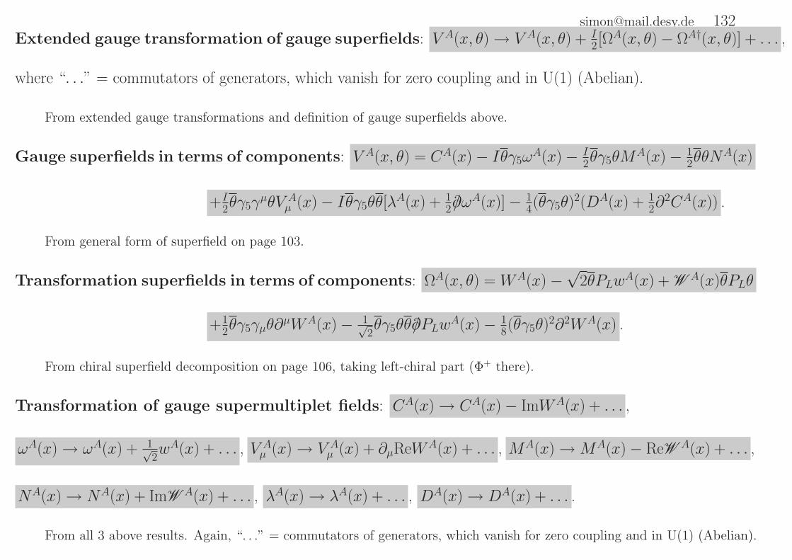
[email protected] 132Extended gauge transformation of gauge superfields: V A(x, θ) → V A(x, θ) + I
2 [ΩA(x, θ) − ΩA†(x, θ)] + . . . ,
where “. . .” = commutators of generators, which vanish for zero coupling and in U(1) (Abelian).
From extended gauge transformations and definition of gauge superfields above.
Gauge superfields in terms of components: V A(x, θ) = CA(x) − Iθγ5ωA(x) − I
2θγ5θMA(x) − 1
2θθNA(x)
+I2θγ5γ
µθV Aµ (x) − Iθγ5θθ[λ
A(x) + 12/∂ωA(x)] − 1
4(θγ5θ)2(DA(x) + 1
2∂2CA(x)) .
From general form of superfield on page 103.
Transformation superfields in terms of components: ΩA(x, θ) = WA(x) −√
2θPLwA(x) + W A(x)θPLθ
+12θγ5γµθ∂
µWA(x) − 1√2θγ5θθ/∂PLw
A(x) − 18(θγ5θ)
2∂2WA(x) .
From chiral superfield decomposition on page 106, taking left-chiral part (Φ+ there).
Transformation of gauge supermultiplet fields: CA(x) → CA(x) − ImWA(x) + . . . ,
ωA(x) → ωA(x) + 1√2wA(x) + . . . , V A
µ (x) → V Aµ (x) + ∂µReWA(x) + . . . , MA(x) →MA(x) − ReW A(x) + . . . ,
NA(x) → NA(x) + ImW A(x) + . . . , λA(x) → λA(x) + . . . , DA(x) → DA(x) + . . . .
From all 3 above results. Again, “. . .” = commutators of generators, which vanish for zero coupling and in U(1) (Abelian).

[email protected] 133Wess-Zumino gauge: CA, ωA,MA, NA = 0 → V A(x, θ) = I
2θγ5γµθV A
µ (x) − Iθγ5θθλA(x) − 1
4(θγ5θ)2DA(x) .
Transformation of supermultiplet fields on page 132: take ImWA(x) = CA(x), wA(x) = −√
2ωA(x), W A(x) = MA(x) − INA(x).
Sufficient for Abelian case because “. . .” = 0. For non-Abelian case, add nth order (in gauge couplings) terms
to ImWA(x), wA(x), W A(x) to cancel nth order terms from commutators of m ≤ n− 1th order terms.
Wess-Zumino gauge is not supersymmetric.
Ensuring δCA, δωA, δMA, δNA = 0 in component field transformations on page 104, requires also having V Aµ , λ
A = 0,
which requires δV Aµ , δλ
A = 0. δV Aµ = 0 satisfied, but δλA = 0 requires DA = 0, i.e. V A = 0.
Gauge invariant L for chiral supermultiplet: 12[Φ
†ΓΦ]D = −12(Dµφ)†Dµφ− 1
2ψLγµDµψL + 1
2F†F
+I√
2ψLtAλAφ− 1
2DAφ†tAφ + h.c. , where covariant derivative Dµ = ∂µ − ItAV
Aµ
(gauge transformation for gauge superfield derived next on page 134).
In Wess-Zumino gauge, Γ(x, θ) = 1 − Iθγ5γµθtAVAµ (x) − 1
2θγ5γµθθγ5γ
νθtAtBVAµ (x)V B
ν (x) + 2Iθγ5θtAθλA(x) + 1
2(θγ5θ)2tAD
A(x).
Then use left-chiral superfield in chiral superfield decomposition on page 106.
Note D term is coefficient of −14(θγ5θ)
2 minus 12∂
2× first “φ” term.

[email protected] 134Gauge transformation of gauge supermultiplet fields: δgaugeV
Aµ (x) = CABCV
Bµ (x)ΛC(x) + ∂µΛ
A(x)
(which is infinitesimal version of transformation of gauge fields on page 66), and
δgaugeλA(x) = CABCλ
B(x)ΛC(x) , δgaugeDA(x) = CABCD
B(x)ΛC(x) (i.e. λA, DA in adjoint representation).
Firstly ΛA(x+) = ΛA(x) + 12(θγ5γµθ)∂
µΛA(x) − 18(θγ5θ)
2∂2ΛA(x). Then gauge transformation of gauge connection on page 131
(using connection from gauge superfields) reads exp[−2tAVA′(x, θ)] = exp[ItAΛA†(x+)] exp[−2tAV
A(x, θ)] exp[−ItAΛA(x+)].
Write as exp[−2tAVA′(x, θ)] = eaeXeb where X = −2tAV
A(x, θ) = −2tA[I2θγ5γµθVAµ (x) − Iθγ5θθλ
A(x) − 14(θγ5θ)
2DA(x)] , and
small quantities b+ a = 2tAImΛA(x+) = −Iθγ5γµθtA∂µΛA(x) , b− a = −2ItAReΛA(x+) = −2ItA[ΛA(x) − 1
8(θγ5θ)2∂2ΛA(x)] .
To first order in a, b, −2tAVA′(x, θ) = X + 1
2 [X, b− a] + b+ a+ . . . and “. . .” means higher order in a, b,
as well as terms of O(Xn)O(b− a) with integer n ≥ 2 which vanish:
since (1, γ5) = PL ± PR, X ∼ θLθR(× further θ factors), while b+ a ∼ θLθR, so O(X2)O(b− a) ∼ θ3Lθ
3R(× . . .) = 0.
So V A′(x, θ) = V A(x, θ) + CABCVB(x, θ)ΛC(x) + I
2θγ5γµθ∂µΛA(x),
compare superfield expansion in Wess-Zumino gauge on page 133.
Wess-Zumino gauge is gauge invariant under ordinary gauge transformations.
Last underlined equation above shows that δCA = δωA = δMA = δNA = 0.
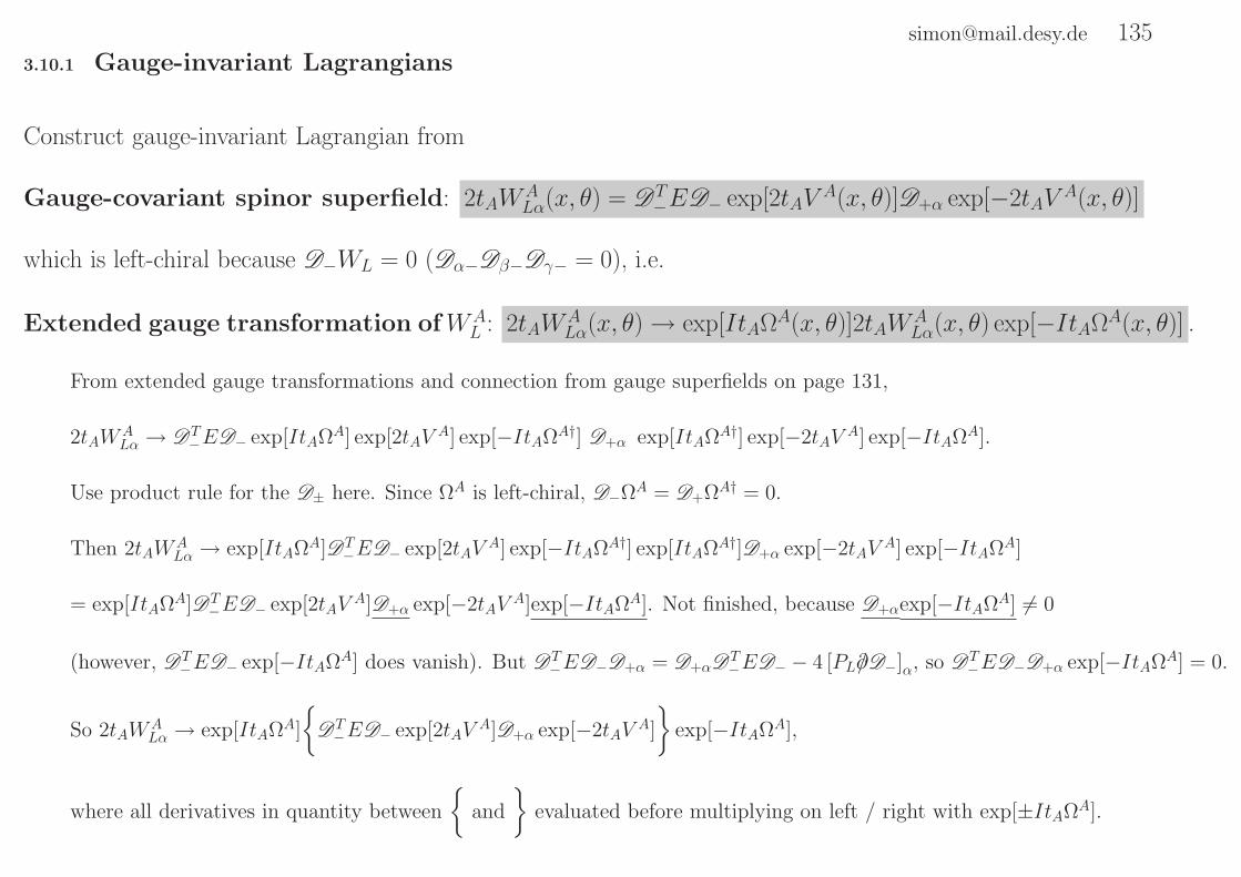
[email protected] 1353.10.1 Gauge-invariant Lagrangians
Construct gauge-invariant Lagrangian from
Gauge-covariant spinor superfield: 2tAWALα(x, θ) = DT
−ED− exp[2tAVA(x, θ)]D+α exp[−2tAV
A(x, θ)]
which is left-chiral because D−WL = 0 (Dα−Dβ−Dγ− = 0), i.e.
Extended gauge transformation ofWAL : 2tAW
ALα(x, θ) → exp[ItAΩA(x, θ)]2tAW
ALα(x, θ) exp[−ItAΩA(x, θ)] .
From extended gauge transformations and connection from gauge superfields on page 131,
2tAWALα → DT
−ED− exp[ItAΩA] exp[2tAVA] exp[−ItAΩA†] D+α exp[ItAΩA†] exp[−2tAV
A] exp[−ItAΩA].
Use product rule for the D± here. Since ΩA is left-chiral, D−ΩA = D+ΩA† = 0.
Then 2tAWALα → exp[ItAΩA]DT
−ED− exp[2tAVA] exp[−ItAΩA†] exp[ItAΩA†]D+α exp[−2tAV
A] exp[−ItAΩA]
= exp[ItAΩA]DT−ED− exp[2tAV
A]D+α exp[−2tAVA]exp[−ItAΩA]. Not finished, because D+αexp[−ItAΩA] 6= 0
(however, DT−ED− exp[−ItAΩA] does vanish). But DT
−ED−D+α = D+αDT−ED− − 4 [PL/∂D−]α, so DT
−ED−D+α exp[−ItAΩA] = 0.
So 2tAWALα → exp[ItAΩA]
DT
−ED− exp[2tAVA]D+α exp[−2tAV
A]
exp[−ItAΩA],
where all derivatives in quantity between
and
evaluated before multiplying on left / right with exp[±ItAΩA].

[email protected] 136Form of WA
L : WAL (x, θ) = λAL(x+) + 1
2γµγνθLF
Aµν(x+) + θTLEθL /DλAR(x+) − IθLD
A(x+) .
Note exp[−2tAVA(x, θ)] = 1 − Iθγ5γµθtAV
Aµ (x) − 1
2θγ5γµθθγ5γ
νθtAtBVAµ (x)V B
ν (x) + 2Iθγ5θtAθλA(x) + 1
2(θγ5θ)2tAD
A(x).
After performing all D± in gauge-covariant spinor superfield on page 135, choose gauge where V Aµ (X) = 0 at given x = X,
gives WAL (X, θ) = λAL(X+) + 1
2γµγνθL(∂µV
Aν (X+) − ∂νV
Aµ (X+)) + θTLEθL/∂λAR(X+) − IθLD
A(X+). Then convert to
gauge covariant form consistent with this, i.e. ∂µVAν − ∂νV
Aµ → FA
µν (the non-Abelian field strength of page 67) and /∂ → /D.
Alternative form of WAL : D+EW
AL = D−EWA
R with /D → /∂, ǫµνρσ∂ρfµν = 0.
Note WAR from WA
L via x+ → x−, R ↔ L, E → −E. Implies form of WAL above, by direct calculation.
Gauge supermultiplet Lagrangian: Lgauge = −12Re([WAT
L EWAL ]F ) = −1
4FAµνF
Aµν − 12λ
A( /Dλ)A + 1
2DADA .
From form of WAL above.
Additional non perturbative part: Lθ = − g2θ16π2Im
([WAT
L EWAL ]F
)= − g2θ
16π2
(Iλ
A/Dγ5λ
A − 14ǫµνρσF
AµνFAρσ)
,
where g is coupling appearing in tA.
Fayet-Iliopolis term: LFI = ξD , where ξ is arbitrary constant, D is for Abelian supermultiplet..
Corresponding action is supersymmetric, because δD = Iαγ5/∂λ is derivative.

[email protected] 137Explicit check that action from gauge supermultiplet Lagrangian Lgauge on page 136 is supersymmetric.
In V Aµ (X) = 0 gauge, component field transformations on page 104 at x = X: δV A
µ = αγµλA, δDA = Iαγ5/∂λ
A, and
δλA = (14F
Aµν[γ
ν, γµ] + Iγ5DA)α where FA
µν = ∂µVAν − ∂νV
Aµ + CABCV
Bµ V
Cν is non-Abelian field strength of page 67.
Then using δ(FAµνF
Aµν) = 2FAµνδF
Aµν etc., δ(FAµνF
Aµν) = 2FAµνα(γν∂µ − γµ∂ν)λA, δ(DADA) = 2IDAαγ5/∂λ
A
and δ(λA
/DABλB) = (δλ
A) /DABλ
B + λA
/DABδλB + λ
A(δ /DAB)λB = 2α[14F
Aµν[γ
µ, γν] + Iγ5D]/∂λA + CABCλAδ( /V B)λC
(we will show CABCλAδ( /V B)λC = 0 later). For this last expression, use [γµ, γν]γρ = −2gµργν + 2gνργµ − 2Iǫµνρσγσγ
5
(expand in 16 matrices on page 45, Lorentz and space inversion invariance limits this to these three terms.
1st coefficient by taking µνρ = 121: [γ1, γ2]γ1 = −2g11γ2, correct because from anticommutation relations for γµ on page 44,
γ1γ2 = −γ2γ1 and γ1 2 = 2. Similarly for µνρ = 211 to get 2nd coefficient. 3rd coefficient from µνρ = 123:
[γ1, γ2]γ3 = −2Iǫ1230γ0γ5, LHS is 2γ1γ2γ3 = −2γ0γ0γ1γ2γ3 = −2Iγ0γ5).
So δ(λA/∂λA) = −FAµνα(γν∂µ − γµ∂ν)λ
A − IǫµνρσFAµναγσγ5∂ρλ
A + 2IDAαγ5/∂λA. 2nd term replaceable, after integration by parts,
by Iǫµνρσ(∂ρFAµν)αγσγ5λ
A, which vanishes since e.g. ǫµνρσ∂ρ∂µVAν = 0, 1st and 3rd terms cancel with δ(FA
µνFAµν) and δ(DADA).
Thus we are left with CABCλAδ( /V B)λC = CABCλ
Aγµλ
CαγµλB = 0,
where antisymmetry of CABC used in 1st step. Last step requires explicit calculation.

[email protected] 138Lagrangian for chiral and gauge supermultiplet fields:
L = −(Dµφ)†n(Dµφ)n − 1
2ψnLγµ(DµψL)n + 1
2DµψnLγµψnL − 1
2∂2f
∂φn∂φmψTnLEψmL − 1
2
(∂2f
∂φn∂φm
)∗ (ψTnLEψmL
)∗
−V (φ) + I√
2ψnL(tA)nmλAφm − I
√2φ†nλ
A(tA)nmψmL − 1
4FAµνF
Aµν − 12λ
A( /Dλ)A + g2θ
64π2ǫµνρσFAµνFAρσ ,
where potential V (φ) = ∂f(φ)∂φn
(∂f(φ)∂φn
)∗+ 1
2
(ξA + φ∗n(tA)nmφm
) (ξA + φ∗k(tA)klφl
).
Sum of gauge invariant L for chiral supermultiplet on page 133, superpotential part of L on page 113 and 3 Lagrangians
on page 136 gives L = 12
[Φ† exp
(−2tAV
A)Φ]D
+ 2Re[f(Φ)]F − 12Re
(WAT
L EWAL
)F− ξADA − g2θ
16π2 Im(WATL EWA
L )F ,
or explicitly (using Majorana conjugation on page 96, e.g. ψR = ψ†PRβ = ψPL = ψTEγ5PL = ψTPLEγ5 = ψTLEγ5)
L = −(Dµφ)†n(Dµφ)n − 1
2ψnγµ(Dµψ)n + F †
nFn − Re ∂2f∂φn∂φm
ψTnEψm + 2Re∂f(φ)∂φn
Fn − 2√
2Im(tA)nmψnLλAφm
+2√
2Im(tA)mnψnRλAφ†m − φ†n(tA)nmφmD
A − ξADA + 12D
ADA − 14F
AµνF
Aµν − 12λ
A( /Dλ)A + g2θ
64π2 ǫµνρσFAµνFAρσ.
Then use field equations for auxiliary fields: Fn = −(∂f(φ)∂φn
)†and DA = ξA + φ∗n(tA)nmφm.

[email protected] 1393.10.2 Spontaneous supersymmetry breaking in gauge theories
Unbroken SUSY vacuum: Fn0 = −[∂f(φ)∂φn
]φ=φ0
= 0 , DA0 = ξA + φ∗n0(tA)nmφm0 = 0 ⇐⇒ V (φ) = 0.
Can write V = F ∗nFn +DADA > 0, so V = 0 (if allowed) is a minimum. In this case, Fn0 = DA
0 = 0.
From left / right transformation on page 107 and component field transformations on page 104,
〈0|δψL = δF = δφ = δλ|0〉 = 0. Argument holds in reverse.
Note: no overconstraining on M φ components: Fn0 = DA0 = 0 is M conditions,
not M +D, where D is dimensionality of group, i.e. A = 1, . . . , D,
because only M −D conditions needed to satisfy Fn0 = ∂f(φ)∂φ
∣∣∣∣φ=φ0
= 0: f(Φ) invariant under extended gauge transformations
on page 131, ∂f(Φ)∂ΩA = 0 = ∂f(Φ)
∂Φn
∂([eItBΩB ]nmΦm)∂ΩA
∣∣ΩC=0
= ∂f(Φ)∂Φn
(ItAΦ)n, i.e. ∂f(φ)∂φn
(tAφ)n = 0, which is already D conditions.

[email protected] 140Existence of any supersymmetric field configuration =⇒ unbroken SUSY vacuum.
From above, SUSY field configuration has V = 0, which is absolute minimum so lower than V for non SUSY field configuration.
(Now let ξA = 0.) To check vacuum is unbroken SUSY, enough to check that ∂f(φ)∂φn
= 0 can be satisfied.
f(φ) has no φ†, so invariant under φ→ eIΛAtAφ with ΛA complex. If ∂f(φ)
∂φn= 0 true for φ, true for φΛ = eIΛ
AtAφ.
Choose ΛA such that φΛ†φΛ minimum (which exists because it is real and positive), i.e. ∂∂ΛA (φΛ†φΛ) ∝ φΛ†
n (tA)nmφΛm = 0,
i.e. there exists a field configuration such that DA = 0, so unbroken SUSY vacuum condition obeyed.

[email protected] 141So break SUSY by
1. Making ∂f∂φ = 0 impossible (already considered on page 128)
or
2. Fayet-Iliopoulos term ξD. Simple example:
2 left-chiral Φ± with U(1) quantum numbers ±e,
so spinor components are left-handed parts of electron / positron.
Then only possibility is f(Φ) = mΦ+Φ−,
so from V defined on page 138, V (φ+, φ−) = m2|φ+|2 +m2|φ−|2 + (ξ + e2|φ+|2 − e2|φ−|2)2,
which cannot vanish for ξ 6= 0, so SUSY broken.
Note U(1) symmetry intact for |ξ| < m2
2e2, since minimum at φ+ = φ− = 0.

[email protected] 142Tree-level mass sum rule: C = 0 , where C =
∑fermionsm
2 −∑bosonsm2. For unbroken/broken SUSY.
Take new scalar fields ∆φn = φn − φn0. Then quadratic part of V defined on page 138 in unitarity gauge φ†(tAφ0) = 0 is
Vquad = 12
(∆φ∆φ∗
)†M 2
0
(∆φ∆φ∗
), where M 2
0 =
(M ∗M + (tAφ0)(tAφ0)
† +DA0 tA . . .
. . . MM ∗ + ((tAφ0)(tAφ0)†)∗ +DA
0 tTA
)
(M defined in tree-level expansion of V on page 114). From Lagrangian for chiral and gauge supermultiplet fields
on page 138, terms bilinear in fermion fields are L1/2 = −12
(ψLλ
)TM
(ψLλ
), where M =
(M I
√2(tAφ0)
∗
I√
2(tAφ0)∗ 0
),
so M †M =
(M †M + 2(tAφ0)(tAφ0)
† . . .
. . . 2φ†0tBtAφ0
). For gauge fields, LV = −V A
µ (M 2V )ABV
Bµ where (M 2V )AB = φ†0tB, tAφ0.
Underlined results above give TrM 20 = 2Tr(M ∗M )+TrM 2
V + 2DA0 TrtA and Tr(M †M) =Tr(M ∗M ) + 2TrM 2
V .
Eliminate Tr(M ∗M ) to get TrM 20 − 2Tr(M †M) + 3TrM 2
V = 2DA0 TrtA.
But trace =∑
eigenvalues, so∑
spin 0 mass2 − 2∑
spin 12mass2 + 3
∑spin 1 mass2 = 2DA
0 TrtA.
1 spin-3 component for scalar boson, 2 for spin-12 fermion, 3 for spin-1 gauge boson,
i.e.∑
fermionsm2 −
∑bosonsm
2 = 2DA0 TrtA
In non-Abelian theories, TrtA = 0. Can have TrtA 6= 0 for U(1) but gives graviton-graviton-U(1) anomaly.
C is coefficient of quadratic divergence in vacuum energy, i.e. breaking SUSY does not affect UV structure.
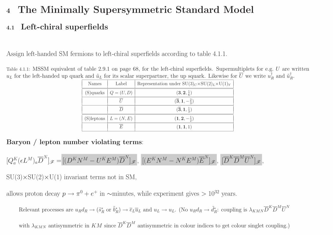
4 The Minimally Supersymmetric Standard Model
4.1 Left-chiral superfields
Assign left-handed SM fermions to left-chiral superfields according to table 4.1.1.
Table 4.1.1: MSSM equivalent of table 2.9.1 on page 68, for the left-chiral superfields. Supermultiplets for e.g. U are writtenuL for the left-handed up quark and uL for its scalar superpartner, the up squark. Likewise for U we write u†R and u†R.
Names Label Representation under SU(3)C×SU(2)L×U(1)Y
(S)quarks Q = (U,D) (3,2, 1
6)
U (3,1,−2
3)
D (3,1, 1
3)
(S)leptons L = (N,E) (1,2,−1
2)
E (1,1, 1)
Baryon / lepton number violating terms:
[QKa (ǫLM)aD
N]F = [(DKNM − UKEM)D
N]F , [(EKNM −NKEM)E
N]F , [D
KDMUN
]F ,
SU(3)×SU(2)×U(1) invariant terms not in SM,
allows proton decay p→ π0 + e+ in ∼minutes, while experiment gives > 1032 years.
Relevant processes are uRdR → (s∗R or b∗R) → eLuL and uL → uL. (No uRdR → d∗R: coupling is λKMNDKDMUN
with λKMN antisymmetric in KM since DKDM
antisymmetric in colour indices to get colour singlet coupling.)

[email protected] 144Rule out some / all baryon lepton number violating terms on page 143 by symmetry, e.g.:
1.) Rule out all by baryon number (B) and lepton number (L) assignments
BU,U = BD,D = ±13, LU,U = LD,D = 0, BN,N = BE,E = 0, LN,N = LE,E = ±1, BθL = BθR = LθL/R = 0.
Or rule out some by requiring only conservation of linear combination, e.g. L, B, B − L etc.
2.) Rule out [DKDMUN
]F by LN = LE = 0, LU = LD = LU = LD = −1, LE = −2.
“Conventional” L for quarks, leptons by taking LθL/R = ±1. L for squarks, sleptons is then unconventional.
But continuous global symmetries are dubious in string theories.
3.) Rule out all by R parity, a discrete global symmetry, = 1 for SM particles and = −1 for their superpartners,
i.e. ΠR = (−1)2s(−1)3(B−L) . Lightest SUSY particle (LSP) (lightest particle with ΠR = −1) completely stable.
Cannot decay into other ΠR = −1 particles (heavier), or into ΠR = 1 particles only (violates R-parity conservation).
Colliders: sparticles produced in pairs.
Non-zero vacuum expectation values for scalar components of NK → charged lepton, charge −e3 quark masses
via 1st, 2nd terms in baryon / lepton number violating terms on page 143, but charge 2e3 quarks remain massless.

[email protected] 145Spontaneous breakdown of SU(2)×U(1) for massive quarks, leptons, W±, Z by Higgs superfields in table 4.1.2:
Table 4.1.2: Required Higgs superfields in the MSSM.
Names Label Representation under SU(3)C×SU(2)L×U(1)Y
Higgs(ino) H1 = (H01 , H
−1 ) (1,2,−1
2)
H2 = (H+
2 , H02 ) (1,2, 1
2)
Higgs-chiral superfield couplings in superpotential [f(Φ)]F : (K,M = generation)
hDKM [(DKH01 − UKH−
1 )DM
]F , hEKM [(EKH01 −NKH−
1 )EM
]F , hUKM [(DKH+2 − UKH0
2)UM
]F .
E.g. last term is just Qa(ǫH2)aU , leads to −GKMu Q
K
L a(ǫφH)†auMR term in LHiggs−fermion on page 70.
Note second Higgs H2 needed for last term, because we need a (1,2, 12) left-chiral superfield. (H†
1 is (1,2, 12), but is right-chiral.)
〈0|φH01|0〉 6= 0 gives mass to d-type quarks and charged leptons, 〈0|φH0
2|0〉 6= 0 gives mass to u-type quarks.
In superpotential part of L on page 113, fermions get mass from first term −12∂2f(φ)∂φn∂φm
ψnRψmL.
So from e.g. first term of Higgs-chiral superfield couplings in superpotential [f(Φ)]F above,
mass term for dK from ∂2f(φ)
∂dKL ∂dK∗R
dK
RdKL = φH0
1dK
RdKL .
For more Higgs superfields, number of H1 and H2 type superfields must be equal.
Higgsinos produce SU(2)-SU(2)-U(1) anomalies: For H1, anomaly ∝∑t23y =
(12g)2 (1
2g′)+
(−1
2g)2 (1
2g′) = 1
2g2g′,
for H2, anomaly ∝∑t23y =
(12g)2 (−1
2g′)+
(−1
2g)2 (−1
2g′) = −1
2g2g′. No anomalies from gauginos, in adjoint representation.

[email protected] 146Most general renormalizable Lagrangian for a gauge theory with R parity or B − L conserved consists of
1. sum of [Φ∗ exp(−V )Φ]D terms for quark, lepton and Higgs chiral superfields,
2. sum of [ǫαβWαWβ]F for gauge superfields,
3. sum of Higgs-chiral superfield couplings in superpotential [f(Φ)]F on page 145, and
4. µ term: Lµ = µ[HT
1 ǫH2
]F
= µ[H+
2 H−1 −H0
2H01
]F
.
µ has no radiative corrections due to perturbative non-renormalization theorem for F term on page 123.
Gauge hierarchy problem on page 80 explicitly solved as follows:
Unbroken SUSY: 1-loop correction to Higgs mass from any particle cancelled by that particle’s superpartner.
For broken SUSY, replace Λ2UV with ∼ ∆mass2 of supermultiplet,
so 1-loop correction to Higgs mass from top is |κt|28π2 ∆m2
s, where ∆m2s is mass splitting between top and stop.
No fine-tuning if this is . 1 TeV, so since |κt|2 ∼ 1, stop mass is <√
8π2 ∼ 10 TeV.
Flavour changing processes suppressed to below experimental bounds if squark masses ∼ equal,
so if gauge hierarchy problem solved by SUSY, all squark masses < 10 TeV.

[email protected] 1474.2 Supersymmetry and strong-electroweak unification
Mentioned in grand unification subsubsection, page 76. Assume SUSY unbroken in most of range < MX .
1-loop modifications to SM βi(gi(µr)) = µrddµrgi(µr) from new SUSY particles, with ns Higgs chiral superfields:
β1 =5ngg
′3
36π2 → g′34π2
(5ng6 + ns
8
)=⇒ 1
g′2(µr)= 1
g′2(MX)+ 1
2π2
(5ng6 + ns
8
)ln(MXµr
)
β2 = g3
4π2
(−11
6 +ng3
)→ g3
4π2
(−9
6 +ng2 + ns
8
)=⇒ 1
g2(µr)= 1
g2(MX)+ 1
2π2
(−3
2 +ng2 + ns
8
)ln(MXµr
)
β3 = g3s4π2
(−11
4 +ng3
)→ g3s
4π2
(−9
4 +ng2
)=⇒ 1
g2s(µr)= 1
g2s(MX)+ 1
2π2
(−9
4 +ng2
)ln(MXµr
).
Take µr = mZ , set√
53g
′(MX) = g(MX) = gs(MX), solution (where e defined on page 72, sin2 θW on page 71)
1. sin2 θW (mZ) =18+3ns+
e2(mZ )
g2s(mZ )(60−2ns)
108+6ns
2. ln(MXmZ
)= 8π2
e2(mZ)
1−8e2(mZ )
3g2s (mZ )
18+ns.
For measured values sin2 θW = 0.231, e2(mZ)4π = (128)−1, g
2s(mZ)4π = 0.118, mZ = 91.2GeV,
equation 1. above gives ns = 2, then equation 2. above gives MX = 2 × 10¹⁶GeV.

2 4 6 8 10 12 14 16 18Log10(Q/1 GeV)
0
10
20
30
40
50
60
α−1
α1
−1
α2
−1
α3
−1
Figure 4.1: 2-loop RG evolution of inverse of αi =g2
i
4πin the SM (dashed) and MSSM (solid). α3(mZ) is varied between 0.113 and 0.123, sparticle mass
thresholds between 250 GeV and 1 TeV.

[email protected] 1494.3 Supersymmetry breaking in the MSSM
In effective MSSM Lagrangian, SUSY must be broken.
SUSY breaking terms must not reintroduce hierarchy problem.
Terms with coupling’s mass dimension ≤ 0 → |κψ|2 − λφ = O(ln ΛUV ) (see page 80), so δm2H ∼ Λ2
UV ln ΛUV .
Superrenormalizable terms (coupling’s mass dimension > 0, ∼ power of some M) → δm2H ∼M 2 ln ΛUV ,
OK provided M ∼ mSUSY . 10 TeV. So SUSY breaking terms must be superrenormalizable, called soft terms.

[email protected] 150Soft SUSY breaking R parity / B − L conserving SM invariant terms:
(Sum over SU(2), SU(3) indices and generations K,M)
1. LSR ⊃∑
S −MS2KMφ
K†S φMS , where S = Q,U,D,L,E superfields and φS their component scalars ,
2. LSR ⊃∑X λXmXλX , where X = gluino, wino, bino ,
3. Trilinear terms: LSR ⊃ −ADKMh
DKM(φKQ )T ǫφH1φ
MD− CD
KMhDKM(φKQ )Tφ∗H2
φMD
−AEKMh
EKM(φKL )T ǫφH1φ
ME− CE
KMhEKM(φKL )Tφ∗H2
φME
−AUKMh
UKM(φKQ )T ǫφH2φ
MU− CU
KMhUKM(φKQ )Tφ∗H1
φMU
where hD,E,UKM defined in Higgs-chiral superfield couplings in superpotential [f(Φ)]F on page 145,
4. LSR ⊃ −12Bµφ
TH2ǫφH1 − 1
2m2H1φ†H1
φH1 − 12m
2H2φ†H2
φH2 where µ defined in µ term on page 146.
Recall Hermitian conjugate is added to L . So LSR ⊃ −ReBµφTH2
ǫφH1
−m2
H1φ†H1
φH1 −m2H2φ†H2
φH2.
Choose H1, H2 superfields’ phases so Bµ real, positive: LSR ⊃ −BµReφTH2
ǫφH1
−m2
H1φ†H1
φH1−m2H2φ†H2
φH2

[email protected] 151To respect approximate symmetries, choose AS
KM , B ∼ 1:
ASKM for chiral symmetry: Reflected by small Yukawa coupling of light quarks.
B for Peccei-Quinn symmetry: Reflected by small µ term on page 146.
CSKM terms involve scalar components of left- and right-chiral superfields,
→ quadratic divergences =⇒ fine-tuning and hierarchy problems.
In fact these divergences from scalar tadpole graphs which disappear into vacuum,
cannot occur since no SM invariant scalars.
Note SM superpartners acquire mass even if no electroweak symmetry breaking (i.e. if SM particles massless).
ASKM , B, CS
KM are arbitrary and complex → > 100 parameters even without CSKM terms.
But expect soft terms to arise from some underlying principle.

[email protected] 152SUSY breaking at tree-level for 3 generations ruled out.
Tree-level mass sum rule on page 142 holds for each set of colour and charge values.
Gives e.g. 2(m2d +m2
s +m2b) ≃ 2(5 GeV)2 =
∑of all masses for bosonic degrees of freedom with charge −e/3.
So each squark mass is <√
2 5 GeV ≃ 7 GeV.
Predicts squark mass(es) too small, would have effect in accurately measured e+e− → hadrons.
This is good, otherwise get fine-tuning: tree-level SUSY breaking would require mass parameterM in Lagrangian.
Would affect all SM masses, so M must coincidentally be ∼ electroweak symmetry breaking scale v = 246 GeV.
No SUSY breaking at tree-level implies no SUSY breaking at all orders.

[email protected] 153SUSY breaking at tree-level for ≥3 generations ruled out.
General argument against tree-level SUSY breaking: Consider first underlined equation on page 142.
To conserve colour and charge, only allowed non-zero DA0 terms are for y of U(1) (D1) and t3 of SU(2) (D2).
Squarks are colour triplets, so have zero vacuum expectation values. So for (uL, uR),
M 20U =
(M ∗
UMU − g′ 16D1 + g 12D2 . . .
. . . MUM ∗U + 2
3g′D1
). For (dL, dR), M 2
0D =
(M ∗
DMD − g′ 16D1 − g 12D2 . . .
. . . MDM ∗D − 1
3g′D1
).
Second underlined equation on page 142 gives mass-squared matrix M ∗UMU for charge 2e
3 quarks
and M ∗DMD for charge −e
3 quarks. Let vx, x = u, d be unit eigenvector for quark of lowest mass, i.e. M ∗XMXvx = m2
xvx.
Then mass2 of lightest charge 2e3 squark <
(0vu∗
)†M 2
0U
(0vu∗
)= m2
u + 23g
′D1,
mass2 of lightest charge −e3 squark <
(0vd∗
)†M 2
0D
(0vd∗
)= m2
d − 13g
′D1 ,
so regardless of value / sign of D1 there is at least one squark lighter than u or d quark.
In fact, since D1 ∼ m2SUSY, get squark with negative mass which breaks colour and charge conservation.
Possible solution is new U(1) gauge superfield, so mass2 of lightest charge (2e3 ,−e
3) squark < (m2u + 2
3g′D1,m
2d − 1
3g′D1) + gD.
[email protected] 154Alternative breaking: Introduce new strong-force-like gauge field, asymptotically free coupling G 2(µr)
8π2 ≃ blnµr/mSUSY
,
so µr ≫ mSUSY gives G (µr) ≪ 1 (SUSY unbroken), µr ∼ mSUSY gives G (µr) ∼ 1 (SUSY broken).
Allows for mSUSY ≪MX without introducing MX into theory as new mass scale.
SUSY broken either non-perturbatively or by scalar field potential with non-zero vacuum expectation value.
To get mSUSY ∼ 10TeV ≪MX , G (MX) does not have to be very small (no fine-tuning).
New force clearly does not interact with SM particles,
so SUSY breaking occurs via 〈0|Fhidden|0〉 6= 0 in hidden sector of particles that interact via new force,
communicated to observed particles by interactions felt by both hidden and observed particles,
namely gravity (gravity-mediated SUSY breaking) or SM interactions (gauge-mediated SUSY breaking):

[email protected] 1551. Gravity-mediated SUSY breaking: mSUSY ∼ 〈0|Fhidden|0〉
MP=⇒
√〈0|Fhidden|0〉 ∼ 1011 GeV. (NoCS
KM terms.)
From dimensional analysis, subject to “no SUSY breaking conditions” mSUSY → 0 as 〈0|Fhidden|0〉 → 0 or MP → ∞.
2. Gauge-mediated SUSY breaking: Messenger particle of mass Mmessenger couples to 〈0|Fhidden|0〉
and to MSSM particles via SM interactions (loops). Then mSUSY ∼ αi4π
〈0|Fhidden|0〉Mmessenger
.
For√
〈0|Fhidden|0〉 ∼Mmessenger, =⇒√
〈0|Fhidden|0〉 ∼ 105 GeV. (Very small CSKM terms.)
Flavour blindness of above SUSY breaking mechanisms simplifies soft terms in Lagrangian at µr = MX .
E.g. in minimal supergravity (mSUGRA), K on page 112, which appears in supergravity Lagrangian,
is diagonal for hidden and observed sectors, i.e. K =∑
i=observed, hidden |Φi|2.
Gives organising principle (for mSUGRA) (recall S = Q,D,U, L,E)
MS2KM = m2
0δKM , m2H1
= m2H2
= m20, mgluino = mwino = mbino = m1/2, AS
KM = A0δKM , CSKM = 0.
This or similar principle expected: small experimental upper bounds on flavour changing, CP violating processes.

[email protected] 156Flavour changing processes allowed because squark, slepton mass matrices not necessarily diagonalised
in same basis as quark, lepton mass matrices.
Most stringent limits for quarks are on K0 −K0
transitions involving dL → gluino + dKL , dKL → gluino + sL,
most stringent limits for leptons are on µ→ eγ decays.
CP violating processes allowed due to many new phases in MSSM, can have large effect at low SM energies.
Upper bound on electric dipole moments of neutron and atoms and molecules
requires CP violating phases . 10−2 or some superpartner masses & 1 TeV.

[email protected] 1574.4 Electroweak symmetry breaking in the MSSM
Consider Higgs H1 and H2 superfields’ scalar components φH1 = (φH01, φH−
1)T and φH2 = (φH+
2, φH0
2)T .
Scalar Higgs potential: V = g2
2
∣∣∣∣φ†H1φH2
∣∣∣∣2
+ g2+g′28
(φ†H1
φH1 − φ†H2φH2
)2
+(m2H1
+ |µ|2)φ†H1φH1 + (m2
H2+ |µ|2)φ†H2
φH2 +BµRe(φTH1ǫφH2) .
From potential in Lagrangian for chiral and gauge supermultiplet fields page 138,
with ξA = 0 and f(H1, H2) = µHT1 ǫH2 (the µ term on page 146),
together with part 4. of LSR in soft SUSY breaking terms on page 150.
V bounded from below: 2|µ|2 +m2H1
+m2H2
≥ Bµ .
Terms in V which are quartic in φH1and φH2
are positive or zero. When positive, V has a minimum.
However, quartic terms vanish when φH1= (φ, 0)T and φH2
= (0, φ)T , and then V = (2|µ|2 +m2H1
+m2H2
)|φ|2 −BµRe(φ2),
which must not go to −∞ as |φ| → ∞.

[email protected] 158Definition of vacuum: 〈0|φH+
2|0〉 = 〈0|φH−
1|0〉 = 0 , 〈0|φH0
i|0〉 = vi real ,
so (m2H1
+ |µ|2)v1 + g2+g′24 (v2
1 − v22)v1 − 1
2Bµv2 = 0 and 1 ↔ 2 . Around vacuum, φH0i
= vi + φi .
Define V neutral = V when charged φH−1
= φH+2
= 0.
Choose minimum φH+2
= 0 by SU(2) rotation. ∂V∂φ
H+2
= 0 =⇒ φH−1
= 0 (or Bµ = −g2
2 φ†H0
1φ†H0
2, but then vi = 0).
Then V = V neutral, where V neutral = g2+g′2
8
(|φH0
1|2 − |φH0
2|2)2
+ (m2H1
+ |µ|2)|φH01|2 + (m2
H2+ |µ|2)|φH0
2|2 −BµRe(φH0
1φH0
2).
Let stationary point of V neutral be at φH0i
= vi, i.e. for φH0i
= vi + φi, must have ∂V neutral
∂φi
∣∣∣∣φi=0
= 0,
i.e. coefficient of term ∝ φi vanishes. Gives (m2H1
+ |µ|2)v∗1 + g2+g′2
4 (v21 − v2
2)v∗1 − 1
2Bµv2 = 0 and 1 ↔ 2.
Last result implies v2 real if v1 real. Adjust relative phase between φH01
and φH02
so that v1 is real.
Parameter relations with v1 and v2: Bµ = m2A sin 2β where tan β = v2
v1, m2
A = 2|µ|2 +m2H1
+m2H2
, and
m2H1
+ |µ|2 = 12m
2A − 1
2(m2A +m2
Z) cos 2β , m2H2
+ |µ|2 = 12m
2A + 1
2(m2A +m2
Z) cos 2β with m2Z = 1
2(g2 + g′2)(v2
1 + v22) .
From definition of vacuum above. Compare mZ here with mZ on page 71.
Limit on β: 0 ≤ β ≤ π2 . Bµ = m2
A sin 2β above, but V bounded from below on page 157 is m2A ≥ Bµ, so 0 ≤ sin 2β ≤ 1.

[email protected] 159Quadratic (mass) terms in V neutral: V neutral
quad = 12m
2Z cos 2β
(|φ1|2 − |φ2|2
)+m2
Z (Re(cos βφ1 − sin βφ2))2
+12m
2A(|φ1|2 + |φ2|2) − 1
2(m2A +m2
Z) cos 2β(|φ1|2 − |φ2|2) −m2A sin 2βRe(φ1φ2) .
Neutral Higgs particle masses: m2A , 0 , m2
H = 12
(m2A +m2
Z +√
(m2A −m2
Z)2 + 4m2Am
2Z sin2 2β
),
m2h = 1
2
(m2A +m2
Z −√
(m2A −m2
Z)2 + 4m2Am
2Z sin2 2β
)(zero mass particle is Goldstone boson).
Real, imaginary parts of φi decouple in V neutralquad (no terms like e.g. Re(φ1)Im(φ2)).
First two masses associated with Im(φ) = (Im(φ1), Im(φ2)): Write Im(φ) dependence of V neutralquad as Im(φ)TM 2
Im(φ)Im(φ),
then M 2Im(φ) =
(12m
2A(1 − cos 2β) 1
2m2A sin 2β
12m
2A sin 2β 1
2m2A(1 + cos 2β)
). Eigenvalues are m2
A and 0, corresponding eigenstates C odd.
So m2A must be positive to ensure φi = 0 is local minimum, i.e. that eigenvalues of ∂2V
∂φi∂φjpositive. Similarly,
last two masses are eigenvalues of M 2Re(φ) =
(12m
2A(1 − cos 2β) + 1
2m2Z(1 + cos 2β) −1
2(m2A +m2
Z) sin 2β−1
2(m2A +m2
Z) sin 2β 12m
2A(1 + cos 2β) + 1
2m2Z(1 − cos 2β)
).
Heaviest neutral scalar: m2H > m2
A,m2Z . Lightest neutral scalar: m2
h < m2A,m
2Z .
Large top to bottom quark mass ratio suggests large tanβ = v2v1
→ m2H ≃ Max(m2
A,m2Z), m2
h ≃ Min(m2A,m
2Z).

[email protected] 160Define V charged = V when φ1 = φ2 = 0.
Quadratic (mass) terms in V charged:
V chargedquad = 1
2(m2W +m2
A)(|φH−
1|2(1 − cos 2β) + |φH+
2|2(1 + cos 2β) + 2 sin 2βRe(φH−
1φH+
2))
, with m2W = 1
2g2(v2
1 + v22) .
Compare mW here with mW on page 71.
Charged Higgs particle masses: 0 , m2C = m2
W +m2A .
V chargedquad = (φH−
1, φH+
2)M 2
C(φ∗H−
1, φ∗
H+2)T , where M 2
C = 12(m
2W +m2
A)
(1 − cos 2β sin 2β
sin 2β 1 + cos 2β
).
Above masses are eigenvalues of M 2C .
Results for neutral and charged scalar fields modified most significantly by radiative corrections from top quark,
which has largest Yukawa couplings to Higgs. Most significant modification to above results are the increases
m2H = 1
2
(m2A +m2
Z + ∆t +√
((m2A −m2
Z) cos 2β + ∆t)2 + (m2A +m2
Z)2 sin2 2β
)
m2h = 1
2
(m2A +m2
Z + ∆t −√
((m2A −m2
Z) cos 2β + ∆t)2 + (m2A +m2
Z)2 sin2 2β
), where ∆t =
3√
2m4tGF
2π2 sin2 βln
M2st
m2t.
By taking stop mass Mst > 300 GeV, tan β > 10, get mh > mZ .
[email protected] 161Condition which leads to electroweak symmetry breaking: 4(m2
H1+ |µ|2)(m2
H2+ |µ|2) ≤ (Bµ)2 .
From parameter relations with v1 and v2 on page 158, 4(m2H1
+ |µ|2)(m2H2
+ |µ|2) = m4A sin2 2β −m2
Z(m2Z + 2m2
A) cos2 2β.
But Bµ = m2A sin 2β, so 4(m2
H1+ |µ|2)(m2
H2+ |µ|2) = (Bµ)2 −m2
Z(m2Z + 2m2
A) cos2 2β, so inequality follows.
These inequalities mean that second derivative matrix of V has negative eigenvalue at SU(2) respecting point φH1= φH2
= 0,
i.e. V unstable (not minimum) there: Quadratic part of scalar Higgs potential on page 157 can be written as four terms
φTM 2φφ, where φ is separately the imainary and real parts of (φH−
1, φH+
2) and (φH0
1, φH0
2), and M 2
φ =
(m2H1
+ |µ|2 ±12Bµ
±12Bµ m2
H2+ |µ|2
).
So mass eigenvalues m2 obey (m2H1
+ |µ|2 −m2)(m2H2
+ |µ|2 −m2) − 14(Bµ)2 = 0,
solutions are 2m2 = 2|µ|2 +m2H1
+m2H2
±√
(2|µ|2 +m2H1
+m2H2
)2 + (Bµ)2 − 4(m2H1
+ |µ|2)(m2H2
+ |µ|2).
Inequality above implies one of these solutions is negative.
Example: For tanβ = ∞ (β = π2), parameter relations with v1 and v2 on page 158
imply m2H1
+ |µ|2 > 0 and m2H2
+ |µ|2 < 0, so electroweak symmetry broken.
Alternatively, radiative corrections give dd lnµr
m2H2
= x hU33 + . . . (hU33 is top quark Yukawa coupling), x > 0.
(Similarly for stop masses, smaller x.) So although m2H2> 0 at µr = MX , may have m2
H2< (≪)0 at µr = v.

[email protected] 1624.5 Sparticle mass eigenstates
Consider gauginos and higgsinos. Particles with different SU(2)×U(1)
but same U(1)e.m. transformation properties can mix after electroweak symmetry breaking.
Neutralinos: 4 neutral fermionic mass eigenstates χ0i , i = 1(lightest), ..., 4,
mixtures of bino, neutral wino, neutral higgsinos.
Bilinear terms in these fields appearing in Lagrangian can be written −12(λ
0)TMχ0λ0, where λ0 = (λbino, λneutralwino, λH01, λH0
2),
Mχ0 =
mbino 0 −cβsWmZ sβsWmZ
0 mwino cβcWmZ −sβsWmZ
−cβsWmZ cβcWmZ 0 −µsβsWmZ −sβcWmZ −µ 0
(sβ = sin β etc.). µ dependent part from µ term on page 146.
mZ dependent part from 1. for Φ = Hi and V = SU(2)×U(1) fields after electroweak symmetry breaking on page 146.
mbino, mwino dependent terms from SUSY breaking terms for gauginos from 2. on page 150.
Mχ0 symmetric, diagonalized by unitary matrix.
χ01 can be LSP, and therefore candidate for cold dark matter.

[email protected] 163Charginos: 4 charged fermionic mass eigenstates χ±
i , i = 1, 2, mixtures of charged winos and charged higgsinos.
Bilinear terms in these fields appearing in Lagrangian can be written −12(λ
+)TMχcλ−,
where λ+ = (λ+charged wino, λH+
2), λ− = (λ−charged wino, λH−
1), Mχc =
(mwino I
√2mWsβ
I√
2mW cβ µ
).
Define λc = (λ+, λ−)T , Mχc =
(0 M †
χc
Mχc 0
), so contribution to Lagrangian including hermitian conjugate
is −12(λ
c)TMχcλc. Squared mass eigenvalues can be obtained from diagonalization of M 2
χc =
(M †
χcMχc 0
0 MχcM†χc
),
gives m2χ+
1,2= m2
χ−1,2
= 12
(m2
wino + 2m2W + |µ|2 ±
√(m2
wino − |µ|2)2 + 4m4W cos2 2β + 4m2
W (m2wino + |µ|2 − 2mwinoRe(µ sin 2β))
).
Slepton, squark mass matrix: m2squark =
(m2Lsquark mT2
LRsquark
m2LRsquark m2
Rsquark
),
where m2L/Rsquark,KM = M
Q/U 2KM + (m2
quark,K +m2Z(T3 −Q sin2 θW ) cos 2β)δKM (no K sum),
MS2KM from 1. on page 150, mquark from unbroken SUSY condition msquark,KK = mquark,K (no K sum),
and term proportional to m2Z from Higgs-chiral superfield couplings in superpotential [f(Φ)]F on page 145.
m2LRsquark,KM = (AU
KM − δKMmquarkµ tan β)mquark . First term from 3. on page 150, second term from∣∣ ∂f∂φH0
1
∣∣2.

Further reading
Stephen P. Martin, hep-ph/9709356 Very topical (not much basics)
— helps you understand what people are talking about
Ian J. R. Aitchison, hep-ph/0505105 Complete derivations up to and including the MSSM
Michael E. Peskin, 0801.1928 [hep-ph] Recent, readable
Steven Weinberg, The Quantum Theory Of Fields III Very complete derivations, quite formal but clear

[email protected] 1645 Supergravity
5.1 Spinors in curved spacetime
Gravity formulated in terms of integer rank matter tensors
and the metric tensor gµν for coordinates xµ over whole of curved spacetime.
Supergravity also involves matter spinors, not generalizable to arbitrary coordinate systems.
So, describe spinor at point X using locally inertial coordinates yaX(x), a = 0, 1, 2, 3,
which transform as ya → y′a = Λab(x)yb (Lorentz transformation)
and have “flat” metric tensor ηab = diag(1, 1, 1,−1).
[email protected] 165Principle of equivalence =⇒ action can be expressed in terms of
1. matter spinors, 2. integer rank matter tensors in yaX(x),
and 3. transformation between locally inertial and general coordinates, described by vierbein:
Vierbein: eaµ(X) =∂yaX(x)
∂xµ
∣∣∣∣x=X
.
Vierbein-metric tensor relation: gµν(x) = ηabeaµ(x)ebν(x) .
Curved space transformation of vierbein: e′aµ(x′) = ∂xν
∂x′µeaµ(x) .
Lorentz transformation of vierbein: eaµ(x) → Λab(x)ebµ(x) .

[email protected] 166A vector may be described by quantities V a(x)
transforming as a vector under local Lorentz transformations (V a(x) → Λab(x)V b(x))
and as a scalar under general coordinate transformations,
or quantities vµ which transform vice versa.
Two types of quantities related by V a = eaµvµ.
Generalize to integer rank tensors.
A spinor may be described by quantities ψα(x)
transforming as a spinor under local Lorentz transformations (ψα(x) → Dαβ(Λ(x))ψβ(x))
but necessarily as a scalar under general coordinate transformations.

[email protected] 167Define covariant derivative of object ψ with a spinor index, Dµψ, to obey
Transformation of covariant derivative: Dµψ → D(Λ)Dµψ under local Lorentz transformations,
Dµψ → ∂xν
∂x′µDνψ under general coordinate transformations.
Achieve this by writing
Covariant derivative of object ψ with a spinor index: Dµψ = ψ;µ + Ωµψ ,
where [Ωµ]αβ(x) = 12I [Jab]αβω
abµ (x),
with Jab the matrix generators of the Lorentz group and ωabµ (x) the spin connection.
and using
Choice of spin connection: ωabµ = gνλeaνebλ;µ . Results in the transformation of covariant derivative above.

[email protected] 1685.2 Weak field supergravity
Work in weak field limit, i.e. eaµ(x) ≃ δaµ, then a→ µ etc.
Weak field representation: eµν(x) = ηµν + 2κφµν , i.e. gµν(x) = ηµν + 2κ(φµν + φνµ) , where κ =√
8πG .
Infinitesimal curved space transformation: xµ → xµ + ξµ(x) .
Infinitesimal Lorentz transformation: Λab(x) = δab + ωab(x) .
Particle content of supergravity: spin-2 graviton hµν = φµν + φνµ and spin-32 gravitino ψµ.
Graviton transformation: φµν(x) → φµν(x) + 12κ
[−∂ξµ(x)
∂xν+ ωµν(x)
]so hµν(x) → hµν(x) + 1
κ
[−∂ξµ(x)
∂xν
].
Follows from performing infinitessimal curved space and Lorentz transformations above.
Gravitino transformation: ψµ(x) → ψµ(x) + ∂µψ(x) .
Required for low energy interactions, similar to requirement of invariance under Aµ(x) → Aµ(x) + ∂µα(x) found on page 55.
Goal: Put φµν, ψµ into one superfield, ξµ, ψ into another.

[email protected] 169Graviton, gravitino as functions of supermultiplet components of
Metric superfield: Hµ(x, θ) = CHµ (x) − I [θγ5]ω
Hµ (x) − I
2
[θγ5θ
]MH
µ (x) − 12[θθ]N
Hµ (x) + I
2 [θγ5γνθ]VH νµ (x)
−I [(θγ5θ)θ](λHµ (x) + 1
2/∂ωHµ (x))− 1
4[θγ5θ]2(DHµ (x) + 1
2∂2CH
µ (x))
,
This is general form of superfield on page 103, but with extra spacetime index µ.
Specifically,
Graviton, gravitino components of metric superfield Hµ: φµν(x) = V Hµν (x) − 1
3ηµνVHλλ (x) ,
12ψµ(x) = λHµ − 1
3γµγρλHρ (x) − 1
3γµ∂ρωHρ (x) .
Graviton, gravitino transformations on page 168 equivalent to
Transformation of metric superfield: Hµ(x, θ) → Hµ(x, θ) + ∆µ(x, θ) , where
Transformation superfield:
∆µ(x, θ) = C∆µ (x) − I [θγ5]ω
∆µ (x) − I
2
[θγ5θ
]M∆
µ (x) − 12[θθ]N
∆µ (x) + I
2 [θγ5γνθ]V∆ νµ (x)
−I [(θγ5θ)θ](λ∆µ (x) + 1
2/∂ω∆µ (x)
)− 1
4[θγ5θ]2(D∆µ (x) + 1
2∂2C∆
µ (x))
.
See later for dependence of these fields on ψ, ξµ of graviton, gravitino transformations on page 168.

[email protected] 170Gravity-matter coupling: Aint = 2κ
∫d4x [HµΘ
µ]D , where
Supercurrent from left-chiral superfields: Θµ = I12
[4Φ†
n∂µΦn − 4Φn∂µΦ†n + (DΦ†
n)γµ(DΦn)].
Supercurrent is a superfield, contains conserved current and energy momentum tensor:
Supercurrent conservation law: γµDΘµ = D 23Im
[M ∂f(Φ)
∂M
]. Use the field equations
(DLDL
)Φn = −4
(∂f(Φ)∂Φn
)∗.
M here defined as follows: Each coupling constant λi in f is written λi = MdM (λi)λi, where λi dimensionless.
SUSY current from supercurrent components: Sµ = −2ωΘµ + 2γµγνωΘν .
Note Sµ is alternative SUSY current on page 127.
Energy-momentum tensor from supercurrent components: Tµν = −12V
Θµν − 1
2VΘνµ + ηµνV
Θλλ , obeys
Energy-momentum tensor conservation law: ∂µTµν = 0 . Follows from supercurrent conservation law above.
Relation between energy-momentum tensor and momentum:∫d3xT 0ν = P ν .
Follows from SUSY transformation of ωΘµ , take time component and integrate over x: I
∫d3xS0, Q
= 2γν
∫d3xT 0ν.
But∫d3xS0 = Q (as in bosonic generator case), then use relation with momentum for any N on page 87.

[email protected] 171Constraint on transformation superfield ∆µ: ∆µ = DγµΞ , where Ξ obeys (DD)(DΞ) = 0 .
Ensures Aint in gravity-matter coupling on page 170 is invariant under transformation of metric superfield on page 169,
follows from supercurrent conservation law on page 170: Let X = 23Im
[M ∂f(Φ)
∂M
].
Then δAint =∫d4x
[Θµ(DγµΞ
)]D
= −∫d4x
[(DΘµ)γµΞ
]D
= −∫ [
(DX)Ξ]D.
But X is a chiral superfield, can be written X = (DD)Ω where Ω is a general superfield.
So δAint =∫d4x
[Ω(DD)(DΞ)
]D
= 0.

[email protected] 172Recall transformation parameters ξµ, ψ in graviton, gravitino transformations on page 168.
Transformation parameter components of transformation superfield:
V ∆µν + V ∆
νµ = − 12κ
[∂ξµ∂xν
+ ∂ξν∂xµ
− 2ηµν∂ξλ
∂xλ
], λ∆
µ − 13γµγ
ρλ∆ρ − 1
3γµ∂ρω∆
ρ = 12∂µψ .
From constraint on transformation superfield ∆µ on page 171, and graviton, gravitino transformations on page 168.
Further constraints on components of transformation superfield: −12ǫνµκσ∂κV
∆νµ = D∆σ + ∂σ∂ρC∆
ρ ,
∂µM∆µ = ∂µN∆
µ = 0 .
Again, from constraint on transformation superfield ∆µ on page 171.
Auxiliary fields: bσ = DHσ + 12ǫνµκσ∂κV
Hνµ + ∂σ∂ρCH
ρ , s = ∂µMHµ , p = ∂µNH
µ , invariant.
From further constraints on components of transformation superfield above.
Choose CHµ = V H
µν − V Hνµ = φµν − φνµ = ωHν = 0 . Then hµν = 2φµν .
Can be done by suitable choice of C∆µ , V ∆
µν − V ∆νµ, ω
∆ν in transformation of metric superfield on page 169.
To summarize, components of superfields are:
Θµ ∋ T κσ, Sσ, Rσ, M , N , Hµ ∋ hκσ, ψσ, bσ, s, p, where Rµ = 2CΘµ , MΘ
µ = ∂µM , NΘµ = ∂µN .
Gravity-matter coupling in terms of components: Aint = κ∫d4x[T κσhκσ + 1
2Sσψσ + Rσb
σ − 2M s− 2N p] .

[email protected] 173For dynamic part of gravitational action, use:
Einstein superfield Eµ: CEµ = bµ , ωEµ = 3
2Lµ − 12γµγ
νLν , MEµ = ∂µs , NE
µ = ∂µp ,
V Eµν = −3
2Eµν + 12ηµνE
ρρ + 1
2ǫνµσρ∂σbρ , λEµ = ∂µγ
νωEν − /∂ωEµ , DEµ = ∂µ∂
νbν − ∂2bµ , where Lν = Iǫνµκργ5γµ∂κψρ ,
and linearized Einstein tensor Eµν = 12
(∂µ∂νh
λλ + ∂2hµν − ∂µ∂
λhλν − ∂ν∂λhλµ − ηµν∂
2hλλ + ηµν∂λ∂ρhλρ
)
= 12κ
(Rµν − 1
2gµνR)
.
Dynamic part of gravitational Lagrangian: LE = 43[EµH
µ]D = Eµνhµν − 1
2ψµLµ − 4
3(s2 + p2 − bµb
µ) .
Invariant under transformation of metric superfield on page 169.
Now put together matter Lagrangian LM , and LE and integrand of Aint above and eliminate auxiliary fields:
Lagrangian of nature: L = LM + Eµνhµν − 1
2ψµLµ + κ[T κσhκσ + 1
2Sσψσ] +3
4κ2(M 2 + N 2 − 1
4RµRµ)
.
Field equations give s = −6κM /8, p = −6κN /8, bµ = −6κRµ/16.
Everything except LM is of order κ2.

[email protected] 174Vacuum energy density: ρVAC = −LVAC = −LM VAC − 3
4κ2(M 2 + N 2).
Only s and p can acquire vacuum expectation values.
Solution to Einstein field equations (ρVAC uniform) for ρVAC ≷ 0 is de Sitter / anti de Sitter space:
spacetime embedded in 5-D space with x25 ± ηµνx
µxν = R2 and ds2 = ηµνdxµdxν ± dx2
5 for ρVAC ≷ 0.
ρVAC < 0 corresponds to O(3,2), which includes N = 1 SUSY,
but ρVAC > 0 corresponds to O(4,1), which excludes unbroken N = 1 SUSY.
In unbroken SUSY, LM VAC = 0 so from vacuum energy density above, ρVAC < 0.
ρVAC < 0 is unstable. However, anti de Sitter space cannot form
since positive energy S1 > |ρVAC| is needed for its surface tension.

[email protected] 175Local supersymmetry: α in definition of superfield on page 101 becomes dependent on x.
Only change is to matter action: δ∫d4xLM = −
∫d4xS
µ(x)∂µα(x) (usual definition of current).
Cancelled by term κ∫d4x1
2Sσψσ in gravity-matter coupling in terms of components on page 172
if SUSY transformation of gravitino modified to: δψµ → δψµ + 2κ∂µα.
But ψµ → ψµ + 2κ∂µα is of same form as gravitino transformation on page 168,
i.e. leaves term −12ψµL
µ in dynamic part of gravitational Lagrangian LE on page 173 unchanged.
So supersymmetric gravity is locally supersymmetric.

[email protected] 1765.3 Supergravity to all orders
Lagrangian of nature (page 173) not supersymmetric at O(κ) (from matter - gravity supermultiplet interaction).
Solution: keep adding terms of higher order in κ to SUSY transformations
until SUSY, local Lorentz and general coordinate transformations form closed algebra,
then keep adding terms to action till it is invariant under all these transformations.
Define Dµ = ∂µ + 18[γa, γb]ω
abµ , ωabµ = eaλe
bν;µg
λν + κ2
4
[ebν(ψµγ
aψν)
+ eaνebρ
(ψνγµψ
ρ)− eaν
(ψµγ
bψν)]
,
This is the covariant derivative on page 167, with a gravitino-dependent term added to the spin connection,
and we have used [Jab]αβ = −I4 [γa, γb]. in the Dirac representation.
γµ = eaµγa , e =√
Detg , Lµ = Iγ5γνDρψσǫµνρσ .

[email protected] 177Then for the metric superfield
Local SUSY transformation of gravity: δψµ = 2κDµα + 2Iγ5(bµ − 1
3γµγρbρ)α + 2
3γµ(s− Iγ5p)α ,
δs = 14e (αγµL
µ) + κ2 (α[Iγ5b
ν − sγν − Ipγ5γν]ψν) , δp = − I
4e (αγ5γµLµ) + κ
2 (α[bν + Isγ5γν − pγν]ψν) ,
δbµ = 3I4e
(αγ5(Lµ − 1
3γµγρLρ))
+ κ2bν (αγνψµ) + Iκ
2
(ψµγ5(s− Iγ5p)α
)− Iκ
4 ǫµνκσbν (αγ5γ
κψσ) , δeaµ = κ (αγaψµ) .
Action for pure supergravity: ISUGRA =∫d4x
[− e
2κ2R− 12ψµL
µ − 4e3
(s2 + p2 − bµb
µ)]
.
s = p = bµ = 0 gives action in absence of matter.
Vierbein curvature tensor from spin connection: Rabµν = ωabµ,ν − ωabν,µ + ωacν ω
bµc − ωacµ ω
bνc .
Vierbein and Riemann-Christoffel curvature tensors: Rabµν = eaκe
bλR
κλµν .

[email protected] 178For matter superfields, first consider general scalar superfield:
First we define
Covariant derivatives: DaC = e µa
[∂µC − Iκ
2
(ψµγ5ω
)],
Daω = e µa
[∂µω + 1
8ωcbµ [γc, γb]ω − Iκbµγ5ω − κ
2 ( /V − Iγ5/∂C −M + Iγ5N)ψµ],
Daλ = e µa
[∂µλ + 1
8ωcbµ [γc, γb]λ + Iκbµγ5λ + κ
8 [γb, γc]ψµFbc − Iκ2 γ5Dψµ
],
Fab = e µa e
νb
[∂µVν + κ
2∂µ(ψνω
)− κ
2
(ψµγνλ
)]− a↔ b ,
then
Local SUSY transformation of scalar supermultiplet:
δC = I (αγ5ω) , δω = [−Iγ5 /DC −M + Iγ5N + /V ]α ,
δM = − (α[λ + /Dω]) + 2κ3 (α[s− Iγ5p + Iγ5b/]ω) , δN = I (αγ5[λ + /Dω]) + 2Iκ
3 (α[s− Iγ5p + Iγ5b/]γ5ω) ,
δVa = (αγaλ) + (αDaω) + κ3 (α[s− Iγ5p + Iγ5b/]γaω) , δλ = −1
4[γa, γb]αFab + IDγ5α , δD = I (αγ5 /Dλ) .

[email protected] 179Chiral superfield: λ = D = 0 , Vν + 1
2κ(ψνω
)= ∂νZ .
Compare with definition of chiral superfield on page 106.
From local SUSY transformation of scalar supermultiplet on page 178, Fab = 0 so δλ = 0, and Daλ = 0 so δD = 0.
Finally δ[Vν + 1
2κ(ψνω
)]= ∂ν (αω).
Otherwise, define left-chiral supermultiplet as on page 106.
Local SUSY transformation of left-chiral supermultiplet: δφ =√
2 (αψL) ,
δψL =√
2(/∂φ)αR − κγµ(ψµψL
)αR +
√2FαL , δF =
√2 (α /DψL) − 2κ
3 (α [s− Ip− Ib/]ψL)
From local SUSY transformation of scalar supermultiplet on page 178.
Recall ω = −Iγ5ψ so /DψL from /Dω from covariant derivatives on page 178.

[email protected] 180D and F terms not locally supersymmetric.
Instead use
Modified D-term: [S]modified D = e
[DS − Iκ
2
(ψµγµγ5λ
S)
+ 4κ3 [−sNS + pMS − bµV S
µ ]
−Iκ3
(ωSγ5 /L
)− κ2
4 ǫµρστV S
σ
(ψργτψµ
)κ2
8 ǫµρστ
(ωSψσ
) (ψργτψµ
) ]− 2κ2
3 CSLSUGRA
and
Modified F -term: [X ]modified F = e[FX + κ√
2
(ψµRγ
µψXL)
+ κ2
4
(ψµR[γµ, γν]ψνR
)φX + 2κ(s− Ip)φX
].
Then
Local SUSY Lagrangian with matter: L = LSUGRA + 12[K(Φ,Φ∗)]modified D + 2Re[f(Φ)]modified F .
Compare with supersymmetric Lagrangian from chiral superfields on page 111.

[email protected] 181Consider other possibilities to add to the Lagrangian.
Supermultiplet I with C = 1, all other fields zero: [I]modified D = −2κ2
3 LSUGRA, i.e. nothing new.
Left-chiral supermultiplet I with φ = 1, all other fields zero: Re([I]modified F ) = e[κ2
4
(ψµ[γ
µ, γν]ψν)
+ 4κs].
Gives gravitino mass mg = cκ2 and
Vacuum energy density: −3κ2c2 .
Add c∫d4xRe([I]modified F ) to action for pure supergravity on page 177, minimize with respect to s, p, bµ.
Then s = 3cκ/2, p = bµ = 0, so c∫d4xRe([I]modified F ) = 3κ2c2
∫d4xe.
Can be used to cancel positive vacuum energy density ρVAC due to SUSY breaking,
making vacuum Lorentz-invariant,
which fixes the relation between gravitino mass mg and ρVAC to mg =√
8πGρVAC/3.

[email protected] 182Let gµν = (1 − κ2K/3)gµν (called a Weyl transformation).
Let Rµν be the curvature tensor calculated using metric gµν, e =√
Detg.
We define the modified Kahler potential d via 1 − κ2
3 d = exp(−κ2d
3
), then define gnm = ∂2d
∂φn∂φ∗m, Lm = ∂f
∂φm+ κ2f ∂d
∂φm
and the potential V = exp(κ2d)[(g−1)nmLmL
∗n − 3κ2|f |2
].
Bosonic part of local SUSY Lagrangian with matter: Lbosonic/e = − 12κ2R
µµ − gnmDµφnD
µφ∗m − V .
From local SUSY Lagrangian with matter on page 180, but with gauge fields included.
Modification with gauge fields: V → V + 12Re(f−1)AB
∂d∂φntAnmφm
(∂d∂φktBklφl
)∗
and Lbosonic/e→ Lbosonic/e− 14Re(fABF
AµνF
Bµν) − 18Im(fABF
AµνF
Bρσǫ
µνρσ) .
Terms quadratic in gaugino fields: L(2)gaugino/e = −1
2RefABλA /DλB + 12 exp(κ2d)Re(g−1)nmLm
(∂fAB∂φn
)∗λAλB .

[email protected] 1835.4 Anomaly-mediated SUSY breaking
O(κ) effect only, results in gaugino masses and Aij and B.
Generalize X defined on page 171 to include gauge superfields W , i.e. X = 23Im
[M ∂f(Φ,W )
∂M
].
Applies also to dimensionless couplings with scale dependence coming from quantum mechanical anomaly.
In gravity-matter coupling in terms of components on page 172, give non-zero expectation values to s and p, so
1st order SUSY-breaking interaction: Lint = −43κRe[(〈s〉 + I〈p〉)M ∂f(φ,λL)
∂M ] .
AX and BX are A- and B- components of X defined in chiral superfield decomposition on page 106.
Then use supercurrent conservation law on page 170 to get M = BX and N = −AX .
Then Lint = 2κIm[(〈s〉 + I〈p〉)AX + IBX ]. Use AX + IBX = φX = X|θ=0 = 2M3I
∂f(φ,λL)∂M .
Gaugino-mass term: Lgaugino mass = Re[mgauginoλ
ALEλ
AL
], where mgaugino = −β(g)
g2κ3 (〈s〉 + I〈p〉) .
Use gauge supermultiplet Lagrangian on page 136 and 1st order SUSY-breaking interaction above.

[email protected] 1845.5 Gravity-mediated SUSY breaking
Includes squark and slepton squared masses, which are of O(κ2).
Assume a new strong force, group G, with scale mW ≪ Λ ≪ mPl,
weak at scale mPl, but strong at scale << mPl.
Φr: includes MSSM superfields, invariant under G,
Zk: hidden sector superfields neutral under SM gauge group, not under G.
In any term in the superpotential, must be at least two of φr or Zk for invariance under the groups,
so form of superpotential (cubic in superfields) must be f(Φ) + f (Z).
[email protected] 185SUSY breaking 1: Scalar fields in Zk of O(Λ), makes φr = O(κΛ2).
Cancellation of large vacuum energy requires some fine-tuning in f at minimum.
Superpotential contains soft SUSY breaking terms, with B = O(1) and A,C small.
Leading non-renormalizable term of O(κΦ2Z2), gives µ-term on page 146 with µ = O(κΛ2).
For κΛ2 = O(1)TeV (MSSM scale),
Λ = O(1011) GeV in range of scales for Peccei-Quinn symmetry breaking
allowed by astronomical observations to resolve the strong CP problem.

[email protected] 186SUSY breaking 2: Hidden sector gauge couplings gives non-perturbative superpotential
for scalar fields y of modular superfields Y ,
which could be e.g. low energy (≪ O(κ−1)) parameters describing compactified extra dimensions of radius O(κ).
After imposing various symmetries f(Φ, Y, Z) = frst(κY )ΦrΦsΦt + fklm(κY )ZkZlZm+ higher powers in Φ, Z.
Gives negligible CD,E,UKM in trilinear terms on page 150.
For Λ = O(1013) GeV (almost OK), gives desired µ = O(κ2Λ3).
Gaugino masses similar to slepton and squark masses.
However, gauge-mediated SUSY breaking yields generation-independent squark and slepton masses.

[email protected] 1876 Higher dimensions
6.1 Spinors in higher dimensions
Lie algebra of O(d− 1, 1): I [Jρσ, Jµν] = −gσνJρµ − gρµJσν + gσµJρν + gρνJσµ .
(Homogeneous) Lorentz group on page 21.
Fundamental spinor representation of O(d− 1, 1): Jµν = −I4 [γµ, γν] ,
where γµ obey Clifford algebra γµ, γν = 2gµν .
This choice obeys Lie algebra of O(d− 1, 1) above.

[email protected] 188d = 2n
Creation/annihilation matrices from γµ: au = 12(γ2u−1 + Iγ2u) , u = 1, 2, . . . , n.
We are defining γ2n = −Iγ0. Creation/annihilation properties au, a†v = δuv and au, av = a†u, a†v = 0
follow from Clifford algebra of the γµ. au and a†u form alternative basis to γµ.
Dimensionality of Clifford algebra space: γµ are 2n × 2n matrices.
Define vectors |0〉 such that a†u|0〉 = 0 and |s1, s2, . . . sn〉 = as11 as22 . . . a
snn |0〉.
Because a2u = 0, si = 0 and 1 only, so there are 2n independent vectors.
Jµν are reducible, sum of 2 irreducible representations Jµν± = Jµν(
1±γ2n+12
).
Define γ2n+1 = Inγ1γ2 . . . γ2n (generalization of γ5 in d = 4).
γ22n+1 = 1 so use representation in which states have with eigenvalues ±1 of γ2n+1.
Using γ2n+1, γµ = 0 for µ = 1, 2, . . . , 2n− 1, 0 (from Clifford algebra), [γ2n+1, Jµν] = 0,
i.e. no mixing between γ2n+1 = ±1 states when acting with Jµν.
In this representation we have block diagonal Jµν = Jµν+ ⊕ Jµν− .

[email protected] 189d = 2n + 1
Exactly as for d = 2n, and now Lorentz generators furnish irreducible representation of Lorentz group.
Everything is as before: Jµν, γµ are the same 2n × 2n matrices as for d = 2n with µ, ν = 1, 2, . . . , 2n− 1, 0, 2n+ 1
and again γ2n+1 = Inγ1γ2 . . . γ2n.
Now the “γ5” matrix γ1γ2 . . . γ2nγ2n+1 = In, i.e. no non-trivial matrix that commutes with Jµν.

[email protected] 1906.2 Algebra
In d dimensions, work in Euclidean space (set xd = Ix0), group is O(d) with unitary representations.
Then for µ(1)ν(1) = d1, µ(2)ν(2) = 23, µ(3)ν(3) = 45, . . ., we have [Jµ(α)ν(α), Jµ(β)ν(β)] = 0.
See Poincare algebra on page 21.
Take any subset Qn of the fermionic generators that form complete representation of Lorentz group.
Can combine Qn so that [Jµ(α)ν(α), Q] = −σµ(α)ν(α)Q (Q is each of the Qn) with σµ(α)ν(α) real numbers.
Q belongs to Qn, where Qn forms complete representation of Lorentz group,
so [Jd1, Qi] = −σd1ij Qj, [J23, Qi] = −σ23ij Qj, . . ., where matrices σAB are Hermitian. Then [J23, [Jd1, Qi]] = σd1ij σ
23jkQk.
Because [Jd1, J23] = 0, this is equal to [Jd1, [J23, Qi]] = σ23ij σ
d1jkQk, i.e. σ23σd1 = σd1σ23.
Diagonalize σd1 with unitary matrix U , i.e. U †σd1U = Λ, where Λij = λiδij (no sum).
Then σ23UΛU † = UΛU †σ23 or ΛΛ = ΛΛ where Λ = U †σ23U , or λiΛij = λjΛij (no sum).
If λi 6= λj, Λij = 0, i.e. Λij is also diagonal.

[email protected] 191Fermionic symmetry generator Q is in fundamental spinor representation of Lorentz group.
Let operator O be of weight w when [Jd1, O] = −wO. So from underlined equation on page 190, Q has w = σd1.
In Minkowski space (J01 = IJd1), [J01, O] = −IwO. Because J †01 = J01, −[J01, O
†] = IwO†, i.e. O† also has weight w.
So Q,Q† has weight 2σd1. From CM theorem, Q,Q† is linear combination of scalars, Pµ and Jµν.
But w(scalars) = 0, and from Poincare algebra on page 21 (with i, j such that 2 ≤ i, j ≤ d− 1),
w(P0 ± P1) = w(J0i ± J1i) = ±1, w(Pi) = w(Jij) = w(J10) = 0,
so 2σd1 = ±1 (not zero, which is excluded by spin-statistics), i.e. σd1 = ±1/2.
In Euclidean formalism, rotational invariance applied to underlined equation above implies all σµ(α)ν(α) = σd1.
So Q must belong to (direct sum of) fundamental spinor representation(s).

[email protected] 192Commutation with momentum: [Q,P µ] = 0 .
[P0 ± P1, [P0 ± P1, Q]] = 0 because |w| = 3/2 or 5/2. So with Q± = [P0 ± P1, Q], [P0 ± P1, [P0 ± P1, Q,Q†]] = −2Q±, Q†±.
But Q,Q† is linear combination of the scalars, Pµ and Jµν, and P0 ± P1 commutes with the scalars and Pµ,
while [P0 ± P1, Jµν] forms linear combinations of Pµ which commutes with the other P0 ± P1 in the underlined equation,
so Q±, Q†± = 0 so Q± = 0, i.e. all Q commute with P0, P1 and by Lorentz invariance all Pµ.
General anticommutation relations: Qn, Qm = ΓµnmPµ + Znm .
[Pµ, Qn, Qm] = 0. But [Jµν, Pρ] 6= 0 so Qn, Qm contains no linear combinations of Jµν.

[email protected] 193Znm are the central charges, conserved scalar generators that commute with everything.
Znm are scalars, so commute with Pµ and Jµν. From general anticommutation relations (page 192), Poincare algebra (page 21),
[Jd1, Qn, Qm] is −(w(Qn) + w(Qm))Qn, Qm = Γ0nmP1 − Γ1nmP0, or −(w(Qn) + w(Qm))[ΓµnmPµ + Znm] = Γ0nmP1 − Γ1nmP0.
Terms in last expression of weight w = 0 give −(w(Qn) + w(Qm))[Znm +∑d−1
i=2 ΓinmPi] = 0.
Spatial rotation of last expression gives −(w(Qn) + w(Qm))Znm = 0. So to allow Znm 6= 0, must have w(Qn) = −w(Qm).
Now let |w(Ql)| 6= |w(Qn(m))| (Ql exists in each irreducible representation for d ≥ 4).
From super-Jacobi identity [Ql, Qm, Qn] + [Qm, Qn, Ql] + [Qn, Ql, Qm] = 0.
Last 2 terms vanish because Qn(m), Ql have some σ 6= 0, i.e. are linear combinations of P ’s but not Z’s,
and P ’s commute with Q’s. So [Ql, Qm, Qn] = [Ql, Zmn] = 0.
But Zmn is a Lorentz scalar, so must commute with all Q’s in the irreducible representation.
So from general anticommutation relations the Z’s commute with each other.
Commutation of central charges and internal symmetry generators: [ti, Zrs] = 0 .
Same derivation as for commutation of central charges and internal symmetry generators on page 89.

[email protected] 1946.3 Massless multiplets
[Q,P µ] = 0, so use eigenstates of P µ. Define little group (pages 24, 33) to leave k = (0, . . . , 0, 1, 1) invariant.
“spin” j is maximum value of any Jµν. Impose condition j ≤ 2 (as on page 56), and one j = 2 particle.
In Hilbert space of little group, only need SUSY generators of weight σd1 = 1/2.
Any SUSY generator Q has weight ±1/2, so Q,Q† has weight ±1 (Q† has same weight as Q from page 191),
i.e. Q,Q† ∝ P 0 ± P 1. But in this Hilbert space P 0 − P 1 = 0.
Further divide generators into two classes with σ23 = ±1/2.
Anticommutation of generators of the same σ23: Qσ23=±1/2, Q′σ23=±1/2 = 0 .
Since all Q for the little group have σd1 = 1/2 and P 0 + P 1 has σd1 = 1, Qσ23=±1/2, Q′σ23=±1/2 ∝ P 0 + P 1.
But P 0 + P 1 has σ23 = 0.

[email protected] 195Limit on number of fermionic generators: N ≤ 32 .
Consider state |λ〉 of spin j and eigenvalue λ > 0 of J23. Let state be annihilated by SUSY generators of σ23 = −1/2
(e.g., but not i.e., when λ = j). States with J23 = λ− k/2 formed by acting on |λ〉 with k SUSY generators of σ23 = 1/2.
(None of these states vanish because acting on them with the adjoints of the k SUSY generators gives back |λ〉.)
There are N /4 SUSY generators with σ23(= σd1) = 1/2 which all anticommute
(see anticommutation of generators of the same σ23 on page 194).
Minimum J23 is then λ− N /8 (for k = N /4). Then impose j ≤ 2 and j − N /8 ≥ −2.
Limit on spacetime dimensionality: d ≤ 11 .
In d = 2n or 2n+ 1 dimensions, a fundamental spinor representation like (a subset of) the SUSY generators has 2n components.
For 2n ≤ 32, need n ≤ 5.

[email protected] 196For d = 11, must have N = 1.
Construct massless multiplet by acting on state with J23 eigenvalue of 2, count number of degrees of freedom.
Gives one graviton and one gravitino. This may be the low energy limit of M -theory.
For d = 10, get massless particle spectrum of 3 kinds of superstring:
Type IIA: 16 generators of each chirality (N = 32)
Type IIB: 32 generators of same chirality (N = 32)
Heterotic: 16 generators of same chirality (N = 16)

[email protected] 1976.4 p-branes
Rank 1 gauge vector fields couple to particles,
but in general rank p+ 1 forms (antisymmetric tensors) couple to extended objects of spatial dimensionality p.
These p + 1 forms are conserved bosonic quantities other than those allowed by CM theorem
so they can appear on the RHS of the SUSY anticommutations.
But SUSY generators still belong to the fundamental spinor representations of the Lorentz group.
Let A... be a p+ 1 form. We now show that the weights of its components are 0 or ±1.
Lorentz transform of A...1... (“1” can only appear once in A... because it is antisymmetric)
is [J1d, A...1...] = (. . .+ (J1d)µ1 + . . .)A...µ.... But (J1d)µν = ±1 when µν = 1d or d1, otherwise (J1d)µν = 0.
So [J1d, A...1...] = A...d.... Likewise [J1d, A...d...] = −A...1.... Thus A...d... ± A...1... has weight ±1.
Also [J1d, A...1...d...] = 0 so A...1...d... has weight 0.
If “. . .” in A... does not contain “1” or “d”, then it has weight 0 because [J1d, A...] = 0,
Then as before the SUSY generators have weight ±1/2.

[email protected] 1987 Extended SUSY
N = 2 global SUSY, massless supermultiplets (or massive “short” supermultiplets discussed on page 94):
Contains supermultiplets (and their CPT-conjugates (helicities reversed)):
• 1 gauge boson of helicity +1, 2 fermions of +1/2 as doublet under SU(2) R-symmetry, 1 boson of 0
and hypermultiplets (and their CPT-conjugates):
• 2 fermions of each helicity ±1/2, 2 bosons of 0 as doublet under SU(2) R-symmetry
Supermultiplet mass limit for N = 2: M ≥ |Z12|/2.
Follows from lower mass bound in extended SUSY on page 94.
We will only consider “short” supermultiplets, so N = 2 supermultiplet mass: M = |Z12|/2 exactly.
See discussion at end of page 94. Equality holds exactly because corrections cannot turn short multiplets into full multiplets.

[email protected] 199Gauge Lagrangian for N = 2: Start with general N = 1 Lagrangian with fields of N = 2 gauge supermultiplet.
An N = 2 theory must have N = 1 SUSY, i.e. N = 2 is a special case of N = 1.
To make this N = 1 Lagrangian become N = 2, impose 2nd SUSY as discrete R-symmetry. We choose
R-symmetry for N = 2 generators: Q1 → Q2 , Q2 → −Q1 .
Leaves result for anticommuting generators on page 88 invariant.
N = 2 supermultiplet ≡ an N = 1 chiral superfield Φ(φ, ψ,F ) + an N = 1 gauge superfield V (V µ, λ,D).
R-symmetry for N = 2 generators above becomes
R-symmetry for N = 2 fields: ψ → λ , λ→ −ψ .
No superpotential is allowed.
Superpotential would depend only on Φ, not V ,
so would give mass and interaction terms for ψ but not λ, not allowed by R-symmetry.

[email protected] 200Define (DµX)A = ∂µXA + CABCVBµXC for X = ψ, λ, φ, and fAµν = ∂µVAν − ∂νVAµ + CABCVBµVCν.
Gauge-invariant Lagrangian for N = 2: L = (Dµφ)∗A(Dµφ)A − 12ψA( /Dψ)A − 1
2λA( /Dλ)A − 14fAµνf
µνA
+√
2CABCψB12(1 − γ5)λAφC −
√2CABCλA
12(1 + γ5)ψCφ
∗B − V (φ, φ∗) + g2θ
64π2ǫµνρσfµνA f ρσA ,
where V (φ, φ∗) = 2CABCReφBImφCCADEReφDImφE is real and positive.
Use N = 1 Lagrangian for chiral and gauge supermultiplet fields on page 138,
combine each chiral and gauge supermultiplet into N = 2 supermultiplet with R-symmetry imposed (i.e. f = 0).
Then set auxiliary fields such that Lagrangian is stationary: FA = 0 and, with ξA = 0, DA = −ICABCφ∗BφC .
N = 2 SUSY has 2 N = 1 SUSYs:
Lagrangian can be seen as N = 1 SUSY with multiplets (φ, ψ,F ) and (V µ, λ,D),
or as N = 1 SUSY with multiplets (φ, λ,F ) and (V µ,−ψ,D).
Use R-symmetry for N = 2 fields on page 199.
Minimum at V = 0 when φA such that CABCReφBImφC = 0 (not only φA = 0).
Such values of φ not equivalent (e.g. give different masses to gauge bosons on breaking gauge symmetries).

[email protected] 201Example: SU(2) gauge theory, CABC = ǫABC . Then
Lagrangian: 1e2
[−(Dµφ)∗A(Dµφ)A − 1
2ψA( /Dψ)A − 2√
2ReǫABCλTALǫψCLφ
∗B − 1
2λA( /Dλ)A]
+ θ64π2ǫµνρσf
µνa f ρσA − V (φ, φ∗) , where V = 2ǫABCReφBImφCǫADEReφDImφE .
From gauge-invariant Lagrangian for N = 2 on page 200, with e absorbed into fields.
For V = 0, consider φ1 = φ2 = 0, φ3 = a. Particles with index 1 and 2 have mass 2|a|, index 3 is massless.
Naively removing massive fields, and dropping the index “3” from now on,
Massless Lagrangian: L = 1e2
[−(∂µa)
∗(∂µa) − 12ψ(/∂ψ) − 1
4fµνfµν − 1
2λ/∂λ]
+ θ64π2ǫµνρσf
µνf ρσ .
Note this is a free field theory, because N = 2 does not allow a superpotential, and there is now just one supermultiplet.
Properly integrating out massive degrees of freedom gives non-renormalizable terms, dominant contributions
at tree-level from interactions of smallest number of fermions, auxilliary fields and derivatives in interaction:
Non-renormalizable low-energy Lagrangian: L = 12 [K(Φ,Φ∗)]D − 1
2Re[T (Φ)(W T
L ǫWL)]F
.
Gauge-covariant spinor superfield on page 135 relates WL to V , and Φ = Φ(a, ψ,F ), V = V (Vµ, λ,D). Count
Feynman diagrams’ energy powers with general L = 12
[K(Φ,Φ†e−2tAVA
)]D
+ 2Re[f(Φ)]F − 12Re
[HAB(Φ)(W T
ALǫWBL)]F
.

Low-energy Lagrangian: L = ∂2K(a,a∗)∂a∂a∗
[−1
2ψ/∂ψ + |F |2 − ∂µa∂µa∗]− Re
(∂3K(a,a∗)∂2a∂a∗ ψψLF
∗)
−12Re
(∂3K(a,a∗)∂2a∂a∗ ψγ
µγ5ψ∂µa)
+ 14∂4K(a,a∗)∂2a∂2a∗ ψψLψψR + 1
4Re(λλLψψL
d2T (a)da2
)− 1
2Re(λλLF
dT (a)da
)
+Re(T (a)
[−1
2λ/∂(1 − γ5)λ− 14fµνf
µν + 18Iǫµνρσf
µνf ρσ + 12D
2])
+√
24 Re
(dT (a)da
[−λγµγνψLfµν + 2IλψLD
]).
Component field expansion of non-renormalizable low-energy Lagrangian on page 201.
N = 2 conditions: (a, ψ,F ) → (a, λ,F ∗) , (Vµ, λ,D) → (Vµ,−ψ,−D) invariance, T = 14πI
dhda , K = Im
(a∗h4π
).
Begin with requirement of invariance under (ψ, λ) → (λ,−ψ). So for coefficients of ψ/∂ψ and λ/∂λ to be equal,
require ∂2K(a,a∗)∂a∂a∗ = Re (T (a)), which is equivalent to expressions above for T (a), K(a, a∗) in terms of some function h(a).
Also insures equality of coefficients of ψγµγ5ψ and λγµγ5λ (the latter appears after integration by parts of 12Re(T (a)λ/∂γ5λ)).
Low-energy Lagrangian in h: L = 14πIm
dhda
[− 1
2ψ/∂(1 − γ5)ψ − 12λ/∂(1 − γ5)λ− ∂µa∂
µa∗ + |F |2
+12D
2 − 14fµνf
µν + 18Iǫµνρσf
µνf ρσ]
+ d2hda2
[−1
2ψψLF∗ − 1
2λλLF + 1√2IλψLD −
√2
4 λγµγνψLfµν
]+ 1
4d3hda3λλLψψL
.
Tree-level h: h =[
4πIe2
+ θ2π
]a . Compare low-energy Lagrangian in h, page 202, with massless Lagrangian, page 201.

[email protected] 203Low-energy action in h: I = 1
8π
∫d4xIm
([Φ∗h(Φ)]D −
[h′(Φ)W T
L ǫWL
]F
).
From non-renormalizable low-energy Lagrangian, page 201, and results for T , K from h in N = 2 conditions, page 202.
Term for SUSY Maxwell equations: ∆I = 18π
∫d4xV Re
([DTLEWL
]D
), V is real superfield.
Gives SUSY Maxwell equations Re(DLEW
AL
)= 0, which is the alternative form of WA
L on page 136.
Full effective action: I = 18π
∫d4xIm
([1
h′(Φ)(WTLEWL)
]F
+ [Φ∗h(Φ)]D
).
Integrate ∆I above by parts, gives ∆I = − 14π
∫d4xIm
([(W T
LEWL)]
F
), where WL = I
4(DTREDR)DLV .
Add to low-energy action in h above, integrate over WL which amounts to setting WL = − WL
h′(Φ) .
Duality: N = 2 effective field theory with scalar field value a and h function h(a)
is physically equivalent to one with scalar field value aD = h(a) and h function h(aD) = −a.
Full effective action above can also be written I = 18π
∫d4xIm
([h′(Φ)(W T
LEWL)]
F+ [Φ∗h(Φ)]D
),
where Φ = h(Φ), h(Φ) = −Φ.
Tree-level dual h: h(aD) = − 1[4πIe2
+ θ2π
]aD . From tree-level h on page 202.


![Lecture notes Introduction to Supersymmetry and Supergravityjlouis/Vorlesungen/SUSY_15/susysugra_15.pdf · 1Textbooks of supersymmetry and supergravity include [1{5]. For review lectures](https://img.dokumen.tips/doc/110x75/5f4932eb921ae62f740d2bba/lecture-notes-introduction-to-supersymmetry-and-supergravity-jlouisvorlesungensusy15susysugra15pdf.jpg)


![Introduction to supergravity - arXiv · supersymmetry, but supergravity is introduced as well. The supergravity review [3] is still, 30 years later, a very good introduction. The](https://img.dokumen.tips/doc/110x75/5ec7a9f876d4fe3f047ef2a9/introduction-to-supergravity-arxiv-supersymmetry-but-supergravity-is-introduced.jpg)


![[Wess Bagger]Supersymmetry and Supergravity](https://img.dokumen.tips/doc/110x75/55cf8eb6550346703b94d652/wess-baggersupersymmetry-and-supergravity.jpg)