Embed Size (px)
Citation preview

Supersymmetry
Lecture in SS 2009 at the KFU Graz
Axel Maas

2

Contents
1 Introduction 1
1.1 Preliminaries . . . . . . . . . . . . . . . . . . . . . . . . . . . . . . . . . . 1
1.2 Why more than the standard model? . . . . . . . . . . . . . . . . . . . . . 2
1.3 A first encounter with supersymmetry . . . . . . . . . . . . . . . . . . . . 2
2 Supersymmetric quantum mechanics 7
2.1 Generators of supersymmetry . . . . . . . . . . . . . . . . . . . . . . . . . 7
2.2 Spectrum of supersymmetric Hamilton operators . . . . . . . . . . . . . . . 10
2.3 Breaking supersymmetry and the Witten index . . . . . . . . . . . . . . . 11
2.4 Interactions and the superpotential . . . . . . . . . . . . . . . . . . . . . . 12
2.5 A specific example: The infinite-well case . . . . . . . . . . . . . . . . . . . 15
3 Grassmann and super mathematics 18
3.1 Grassmann numbers . . . . . . . . . . . . . . . . . . . . . . . . . . . . . . 18
3.2 Superspace . . . . . . . . . . . . . . . . . . . . . . . . . . . . . . . . . . . . 20
3.2.1 Linear algebra . . . . . . . . . . . . . . . . . . . . . . . . . . . . . . 20
3.2.2 Analysis . . . . . . . . . . . . . . . . . . . . . . . . . . . . . . . . . 23
4 Non-interacting supersymmetric quantum field theories 26
4.1 Fermions . . . . . . . . . . . . . . . . . . . . . . . . . . . . . . . . . . . . . 26
4.1.1 Fermions, spinors, and Lorentz invariance . . . . . . . . . . . . . . 27
4.2 The simplest supersymmetric theory . . . . . . . . . . . . . . . . . . . . . 32
4.3 Supersymmetry algebra . . . . . . . . . . . . . . . . . . . . . . . . . . . . . 34
4.3.1 Constructing an algebra from a symmetry transformation . . . . . . 34
4.3.2 The superalgebra . . . . . . . . . . . . . . . . . . . . . . . . . . . . 36
4.3.3 Supermultiplets . . . . . . . . . . . . . . . . . . . . . . . . . . . . . 40
4.3.4 Off-shell supersymmetry . . . . . . . . . . . . . . . . . . . . . . . . 42
i

ii CONTENTS
5 Interacting supersymmetric quantum field theories 46
5.1 The Wess-Zumino model . . . . . . . . . . . . . . . . . . . . . . . . . . . . 46
5.1.1 Majorana form . . . . . . . . . . . . . . . . . . . . . . . . . . . . . 50
5.2 Feynman rules for the Wess-Zumino model . . . . . . . . . . . . . . . . . . 51
5.3 The scalar self-energy to one loop . . . . . . . . . . . . . . . . . . . . . . . 54
6 Superspace formulation 58
6.1 Super translations . . . . . . . . . . . . . . . . . . . . . . . . . . . . . . . . 58
6.2 Coordinate representation of super charges . . . . . . . . . . . . . . . . . . 61
6.2.1 Differentiating and integrating spinors . . . . . . . . . . . . . . . . 61
6.2.2 Coordinate representation . . . . . . . . . . . . . . . . . . . . . . . 62
6.3 Supermultiplets . . . . . . . . . . . . . . . . . . . . . . . . . . . . . . . . . 63
6.4 Other representations . . . . . . . . . . . . . . . . . . . . . . . . . . . . . . 65
6.5 Constructing interactions from supermultiplets . . . . . . . . . . . . . . . . 66
7 Supersymmetric gauge theories 69
7.1 An interlude: Non-supersymmetric gauge theories . . . . . . . . . . . . . . 69
7.1.1 Abelian gauge theories . . . . . . . . . . . . . . . . . . . . . . . . . 69
7.1.2 Non-Abelian gauge theories: Yang-Mills theory . . . . . . . . . . . 71
7.2 Supersymmetric Abelian gauge theory . . . . . . . . . . . . . . . . . . . . 72
7.3 Supersymmetric Yang-Mills theory . . . . . . . . . . . . . . . . . . . . . . 74
7.4 Supersymmetric QED . . . . . . . . . . . . . . . . . . . . . . . . . . . . . 77
7.5 Supersymmetric QCD . . . . . . . . . . . . . . . . . . . . . . . . . . . . . 81
8 Supersymmetry breaking 84
8.1 Dynamical breaking . . . . . . . . . . . . . . . . . . . . . . . . . . . . . . . 85
8.1.1 The O’Raifeartaigh model . . . . . . . . . . . . . . . . . . . . . . . 86
8.1.2 Spontaneous breaking of supersymmetry in gauge theories . . . . . 89
8.2 Explicit breaking . . . . . . . . . . . . . . . . . . . . . . . . . . . . . . . . 91
9 A primer on the minimal supersymmetric standard model 94
9.1 The supersymmetric minimal supersymmetric standard model . . . . . . . 94
9.2 Breaking the supersymmetry in the minimal supersymmetric standard model100
9.3 MSSM phenomenology . . . . . . . . . . . . . . . . . . . . . . . . . . . . . 102
9.3.1 Coupling unification and running parameters . . . . . . . . . . . . . 102
9.3.2 The electroweak sector . . . . . . . . . . . . . . . . . . . . . . . . . 107
9.3.3 Mass spectrum . . . . . . . . . . . . . . . . . . . . . . . . . . . . . 114

Chapter 1
Introduction
1.1 Preliminaries
The prerequisites for this courses are quantum mechanics and quantum field theory. The
necessary basics can also be obtained in parallel in the lectures by H. Gausterer on rel-
ativistic quantum mechanics and quantum field theory and the one of B.-J. Schafer on
theoretical elementary particles to some extent.
There are quite a number of good books on supersymmetry. This lecture is largely
based on
• Supersymmetrie by H. Kalka and G. Soff (Teubner)
• Supersymmetry in particle physics by I. Aitchison (Cambridge)
• The quantum theory of fields III (as well as I and II) by S. Weinberg (Cambridge)
• Fields by W. Siegel (available for free from arxiv.org/abs/hep-th/9912205)
• Supersymmetry and supergravity by J. Wess and J. Bagger (Princeton)
There are also a number of reviews on the topic available on the arXiv and in journals.
Particular recommendable are
• A Supersymmetry primer by S. Martin (arxiv.org/abs/hep-ph/9709356)
• TASI 2002 lectures: Nonperturbative supersymmetry by J. Terning (arxiv.org/abs/hep-
th/0306119)
• The Search for Supersymmetry: Probing Physics Beyond the Standard Model by H.
Haber and G. Kane (Phys.Rept.117:75-263,1985)
1
2 CHAPTER 1. INTRODUCTION
• Supersymmetry, Supergravity and Particle Physics by H. Niles (Phys.Rept.110:1-
162,1984)
which, however go significantly beyond the scope of this lecture.
1.2 Why more than the standard model?
During the last couple of years a number of experimental observations have been made,
which cannot be explained in the framework of the standard model, even when augmented
with classical general relativity. Among these are the fact that the universe is currently
accelerated expanding, as has been deduced from several observables. Furthermore its
density is essential the critical one and thus it will expand eternally. The simplest ex-
planation in both cases would be the existence of additional particles and fields. Also
the period of inflation at very early times would be easiest to understand if particles and
interactions beyond the standard model would be present.
It should be noted that the mass of neutrinos does not require any conceptual new
contribution to the standard model other than some additional parameters.
Finally, the standard model itself is not a mathematical consistent theory for all energy
scales. At some scale it breaks down, an artifact of which is the necessity of renormaliza-
tion. Also, the inclusion of gravity at short distances is not achieved yet.
Hence, there are quite enough reasons to suspect that there is more than the standard
model. One of the hottest candidate for the close vicinity in terms of accessible energy
scales are theories embodying (broken) supersymmetry. The aim of this lecture is to
introduce the concepts necessary for this type of extension.
1.3 A first encounter with supersymmetry
Supersymmetry is a symmetry which links the two basic types of fields one encounters
in the standard model: bosons and fermions. In particular, it is possible to introduce
operators which change a boson into a fermion and vice versa. Supersymmetric theories are
then theories which are invariant under these transformations. This entails, of course, that
such theories necessarily include both, bosons and fermions. In fact, it turns out that the
same number of bosonic and fermionic degrees are necessary to obtain a supersymmetric
theory. Hence to each particle there should exist a super-partner. Superpartners of bosons
are usually denoted by the ending ino, so for a bosonic gluon the fermionic superpartner is
called gluino. For the superpartners of fermions an s is put in front, so the super-partner
of the fermionic top quark is the bosonic stop (and for quarks in general squarks).

1.3. A FIRST ENCOUNTER WITH SUPERSYMMETRY 3
Besides the conceptual interest in supersymmetric theories there is a number of phe-
nomenological consequences which make these theories highly attractive. The most in-
teresting of these is that quite a number of divergences, which have to be removed in
ordinary quantum field theories by a complicated process called renormalization, drop out
automatically. A simple example for this concept is given by an infinite chain of harmonic
oscillators. The Hamilton function for a harmonic oscillator is given by1
HB =p2
2m+m
2x2, (1.1)
where energies and frequencies are measure in units of the mass. It is useful to replace the
operators p and x with the bosonic creation and annihilation operators a and a+
a+ =
√
m
2
(
x− ip
m
)
a =
√
m
2
(
x+ ip
m
)
These operator fulfill the commutation relations
[a, a+] = aa+ − a+a = 1 (1.2)
[a, a] = [a+, a+] = 0.
which follow directly from the canonic commutation relations
[x, p] = i.
Replacing p and x in (1.1) with these new operators yields
HB =1
2
(
a+a+ aa+)
(1.3)
Using the commutation relation (1.2) yields the bosonic harmonic oscillator
HB = a+a+1
2
A noninteracting chain of these operators is therefore described by the sum
HB =
N∑
n=1
(
a+a +1
2
)
.
If the number of chain elements N is sent to infinity, the contribution from the vacuum
term diverges. Of course, in this simple example it would be possible to measure everything
1Everything will be in natural units, i. e., ~ = c = kB = 1.
4 CHAPTER 1. INTRODUCTION
with respect to the vacuum energy, and just drop the diverging constant. However, imagine
one adds a harmonic oscillator, which has fermionic quanta instead of bosonic ones. Such
an oscillator is most easily obtained by replacing in the result (1.3) with
HF =1
2(b+b− bb+)
and the bosonic creation and annihilation operators by their fermionic counterparts b+
and b. This form can be motivated by introducing fermionic coordinates, but this will not
be done here. These satisfy anti-commutation relations
{b, b+} = bb+ + b+b = 1 (1.4)
{b, b} = {b+, b+} = 0.
Using these relations, the Hamiltonian is given by
HF =M∑
n=1
(
b+b− 1
2
)
In this case the vacuum energy is negative. Now, adding both systems with the same
number of degrees of freedom, N = M , the resulting total Hamiltonian
H = HB +HF =
N∑
n=1
(
a+a+ b+b)
(1.5)
has no longer a diverging vacuum energy. Actually, the Hamilton operator (1.5) is one of
the simplest supersymmetric systems. Supersymmetry here means that if one exchanges
bosons for fermions the Hamilton operator is left invariant. This will be discussed in
detail below. The mechanism to cancel the vacuum energy is a consequence of supersym-
metry, and this mechanism is one of the reasons which make supersymmetric theories very
interesting.
From this cancellation it is also possible to obtain a ’natural’ explanation why scalar
particles should be of about the same mass as the other particles in a theory, as will be
discussed in detail much later.
There are some other reasons why supersymmetric theories should be interesting:
• There exists a theorem that without supersymmetry it is not possible to embed the
standard model (Lie groups) and general relativity (Poincare group) into a non-
trivial (i.e. any other than a direct product) common structure (Coleman-Mandula
theorem)
• Supersymmetric theories arise necessarily in the context of string theories

1.3. A FIRST ENCOUNTER WITH SUPERSYMMETRY 5
• Supersymmetry provides a simple possibility to extend the standard model
• Supersymmetry can be upgraded to include also gravity
• Supersymmetry predicts relations between coupling constants which seem without
relation without supersymmetry
• Supersymmetry provides such stringent constraints that many results can be shown
exactly
In particular, it is widely expected that supersymmetry should be manifest at the 1-10
TeV scale, as this is the most likely range for the simplest extension of the standard model
such that one ends up with the known particles with the right properties.
However, there are also several reasons which make supersymmetry rather suspect.
The most important one is that supersymmetry is not realized in nature. Otherwise the
unambiguous prediction of supersymmetry would be that for every bosonic field (e. g. the
photon) an object with the same mass, but different statistic (for the photon the spin-1/2
photino) should exist, which is not observed. The common explanation for this is that
supersymmetry in nature has to be broken either explicitly or spontaneously. However,
how such a breaking could proceed such that the know standard model emerges is not
known. It is only possible to parametrize this breaking, yielding a enormous amount of
free constants and coupling constants, for the standard model more than a hundred, while
the standard model has only about thirty.
In the following chapter 2, the first encounter will be with supersymmetry in quantum
mechanics. After this, a short preparation in Grassmann mathematics will be made in
chapter 3, which will be necessary at many places. Then, things will turn to the first and
simpelst supersymmetric theory, a non-interacting one in chapter 4. Interactions in the
simpelst interacting case, the Wess-Zumino model, will be introduced in chapter 5. After
this first encounter with supersymmetric field theories the concept of superspace will be
introduced in chapter 6, which is very useful in constructing supersymmetric theories. To
be able to discuss supersymmetric extensions of the standard model, the introduction of
supersymmetric gauge theories is necessary, which will be done in chapter 7. Also necessary
to extend the standard model is supersymmetry breaking, which will be discussed in
chapter 8. This is then enough to introduce the minimal supersymmetric standard model
in chapter 9.
As a last remark of this introductory chapter it should be mentioned that supersym-
metry offers also technical methods which can be used even if the underlying theory itself
is not supersymmetric (which is done, e. g., in nuclear physics). So the use of supersym-

6 CHAPTER 1. INTRODUCTION
metric concepts extends far beyond just possible extensions of the standard model. An
example for this will also be discussed in the next chapter.

Chapter 2
Supersymmetric quantum mechanics
Supersymmetry is not a concept which requires either a field theory nor does it require
special relativity. Its most simple form it takes in nonrelativistic quantum mechanics.
However, as fermions are involved, quantum effects are necessary. Such things as spin
1/2-objects, and thus fermions, cannot be described in the context of a classical theory.
2.1 Generators of supersymmetry
To be able to discuss a supersymmetric theory, it is of course necessary to have a Hilbert
space which includes both bosons and fermions. One example would be the Hilbert space
of the harmonic oscillator with only one element, the simplification of (1.5),
H = a+a + b+b. (2.1)
The Hilbert space of this Hamilton operator is given by
|nBnF > (2.2)
where nB is the number of bosons and nF is the number of fermions. Note that no
interaction between bosons and fermions occur. Such an interaction is not necessary to
obtain supersymmetry. However, supersymmetry imposes very rigid constraints on any
interactions appearing in a supersymmetric theory, as will be seen later. Furthermore, the
number of degrees of freedom is the same: one bosonic and one fermionic oscillator.
The conventional bosonic creation and annihilation operators a+ and a now act as
a+|nBnF > =√nB + 1|nB + 1nF >
a|nBnF > =√nB|nB − 1nF >
a|0nF > = 0.
7

8 CHAPTER 2. SUPERSYMMETRIC QUANTUM MECHANICS
The number of bosonic quanta in the system therefore ranges from 0 to infinity. Due to
the Pauli principle the action of the fermionic creation and annihilation operators b+ and
b is much more limited. The only possibilities are
b+|nB0 > = |nB1 >
b|nB1 > = |nB0 >
b+|nB1 > = b|nB0 >= 0.
Thus, there can be only either zero or one fermionic quanta in this system. This also
delivers the complete spectrum of the theory, which is given by
H|nBnF >= nB + nF .
Now, supersymmetry is based on a relation between fermions and bosons. Therefore,
it will be necessary to introduce operators which can change a boson into a fermion. Such
operators can be defined by their action on the states as
Q+|nBnF > ∼ |nB − 1nF + 1 > (2.3)
Q−|nBnF > ∼ |nB + 1nF − 1 > .
Note that since the maximum number of fermionic quanta is 1, Q+ annihilates the state
with one fermionic quanta, just as does the fermionic creation operator. Furthermore,
the operator Q− annihilates the fermionic vacuum, and Q+ the bosonic vacuum, where
vacuum is the state with zero quantas.
Now Q+ and Q− form symmetry transformation operators. However, for a theory
to be supersymmetric, its Hamilton operator must be invariant under supersymmetry
transformations, i. e.,
[H,Q±] = 0. (2.4)
To be able to check this, it is necessary to deduce the commutation relations of the bosonic
and fermionic annihilation operators with Q±. For this an explicit form of Q± in terms of
a and b is necessary. Based on the action on the base state (2.3) it can be directly inferred
that
Q+ = ab+ (2.5)
Q− = a+b.
is adequate. From this also follows that Q+± = Q∓, and both operators are adjoint to each
other. Testing now the condition (2.4) yields for Q+
[a+a+ b+b, ab+] = a+aab+ − ab+a+a+ b+bab+ − ab+b+b. (2.6)

2.1. GENERATORS OF SUPERSYMMETRY 9
Since to consecutive fermionic creation or annihilation operators always annihilate any
state, it follows that
b+b+ = bb = 0.
This property of operators is called nilpotency, the operators are nilpotent. This is a very
important concept, and will appear throughout this lecture. However, currently this only
implies that the last term in (2.6) is zero. Using the brackets (1.2) and (1.4), it then
follows
b+a+aa− b+a− b+a+aa + ab+ − ab+b+b = b+a− ab+ = 0. (2.7)
Here, once more nilpotency was used, and the fact that bosonic and fermionic creation and
annihilation operators commute. The same can be repeated for Q+. Hence the combined
oscillator (2.1) is supersymmetric, and is called the supersymmetric oscillator. In fact this
could be seen easier, as it is possible to rewrite (2.1) in terms of Q± as
H = a+a+ b+b+ a+ab+b− b+ba+a
= aa+b+b+ a+abb+
= {ab+, a+b} = {Q+, Q−}.
From this it follows directly that
[H,Q+] = [Q+Q−, Q+] + [Q−Q+, Q+]
= Q+Q−Q+ −Q+Q+Q− +Q−Q+Q+ −Q+Q−Q+ = 0
This vanishes, as the operators Q± inherit the property of nilpotency directly from the
fermionic operators. This can be repeated for Q−, yielding the same result. As a conse-
quence, any system which is described by the Hamilton operator {Q+, Q−}, where these
can now be a more complex operator, is automatically supersymmetric.
The only now not manifest property is the hermiticity of the Hamilton operator. Defin-
ing the hermitian operators
Q1 = Q+ +Q−
Q2 = i(Q− −Q+)
this can be remedied. By explicit calculation it follows that
H = Q21 = Q2
2. (2.8)
Note that the hermitian operators Q1 and Q2 are no longer nilpotent. Also, since energy
eigenstates are not changed by the Hamiltonian this implies that performing twice the su-
persymmetry transformation Q1 or Q2 will return the system to its original state. Finally,
this implies that the supercharge of a system is an observable quantity.

10 CHAPTER 2. SUPERSYMMETRIC QUANTUM MECHANICS
Furthermore, it can be directly inferred that
{Q1, Q2} = 0.
It is then possible to formulate the supersymmetric algebra of the theory as
[H,Qi] = 0 (2.9)
{Qi, Qj} = 2Hδij.
This algebra is always available when the Hamilton operator takes the form (2.8), which
will be the case in the following. These algebras are often labelled with the number N of
linearly independent generators of supersymmetric transformations. In the present case
this number is N = 2.
2.2 Spectrum of supersymmetric Hamilton operators
There are quite general consequences which can be deduced just from the algebra (2.9),
which implies the form (2.8) of the Hamilton operator. Note that the only properties
which have been used in the calculations previously of the supersymmetric operators were
their nilpotency in the form of Q±, and so they are not restricted to simple harmonic
oscillators.
The first general consequence is that the spectrum is non-negative. This follows trivially
from the fact that (2.8) can be written as the square of a hermitian operator, which has
real eigenvalues. Given , e. g., that |q > is an eigenstate with eigenvalue q to the operator
Q1, it follows immediately that
H|q >= Q21|q >= Q1q|q >= q2|q >
and thus |q > is an energy eigenstate with energy q2, which is positive or zero by the
hermiticity of Q1. Furthermore, let Q2 act on |q >, yielding
Q2|q >= |p > .
This state is in general not an eigenstate of Q1, although it is necessarily by virtue of (2.8)
an eigenstate of Q21. However, acting with Q1 on |p > yields
Q1|p >= Q1Q2|q >= −Q2Q1|q >= −qQ2|q >= −q|p > . (2.10)
Here, it was assumed that q is not zero. Therefore, it is in fact an eigenstate, but to the
eigenvalue −q, |p >= |− q >, so it is different from the original state |q >. Therefore, this
state is also an eigenstate of the Hamilton operator to the same eigenvalue. Hence, for all
non-zero energies the spectrum of the Hamilton operator is doubly degenerate.

2.3. BREAKING SUPERSYMMETRY AND THE WITTEN INDEX 11
2.3 Breaking supersymmetry and the Witten index
If a symmetry is exact, its generator G not only commutes with the Hamilton operator
[H,G] = 0, (2.11)
but the generator must also annihilate the vacuum, i. e., the vacuum |0 > may not be
charged with respect to the generator,
G|0 >= 0.
Otherwise, the commutator relation (2.11) would fail when applied to the vacuum1
[H,G]|0 >= HG|0 > −GH|0 >= HG|0 > .
If the vacuum would be invariant under G, the only other alternative to maintain the
commutator relation, is that it also has to leave all other states invariant, and that it is a
symmetry of the system. It then follows that supersymmetry is exact if
Q1|0 >= 0 or Q2|0 >= 0.
This furthermore implies that if supersymmetry is unbroken the ground state has in fact
energy zero. It will be shown below that this state has to be unique. It should be noted
that there is a peculiarity associated with the fact that the Hamilton operator is just the
square of the generator of the symmetry. Since if supersymmetry is broken
Qi|0 > 6= 0 ⇒ Q2i |0 > 6= 0 (2.12)
the ground state can no longer have energy zero, but must have a non-zero energy. There-
fore it is also doubly degenerate. Hence, the fact whether the ground state is degenerate
or not is therefore indicative of whether supersymmetry is broken or not. This is described
by the Witten index
∆ = tr(−1)NF .
NF is the particle number operator of fermions
NF = b+b.
Therefore, this counts the difference in total number of bosonic and fermionic states
∆ =∑
(
< nF = 0|(−1)NF |nF = 0 > + < nF = 1|(−1)NF |nF = 1 >)
= nB − nF
1It is assumed that the energy is normalized such that the vacuum has energy zero.

12 CHAPTER 2. SUPERSYMMETRIC QUANTUM MECHANICS
where nB is the total number of bosonic states and nF is the total number of fermionic
states. All states appear doubly generate except at zero energy. Furthermore, these
degenerate states are related by a supersymmetry transformation, and thus have differing
fermion number. Hence, the Witten index is reduced to the difference in number of states
at zero energy,
∆ = nB(0) − nF (0).
It is therefore only nonzero if supersymmetry is intact, and zero if not.
2.4 Interactions and the superpotential
To obtain a non-trivial theory, it is necessary to modify the theory. To preserve the
previous results, and obtain a supersymmetric theory, it will be necessary to keep the
operator Q± nilpotent and fermionic. This can be obtained by replacing the definition
(2.5) by
Q+ = Ab+
Q− = A+b,
where the operators A and A+ are arbitrary bosonic functions of the original operators
a and a+. In principle, they may also depend on bosonic quantities formed from b and
b+, like b+b. These would not spoil the nilpotency. For simplicity, this possibility will be
ignored here.
In this case NB is in general no longer a good quantum number, but NF is trivially.
So all states can be split into states with either NF = 0 or NF = 1, and can furthermore
be labelled by their energy,
H|EnF > = E|EnF >
NF |EnF > = nF |EnF > .
It is therefore useful to rewrite the states as
|EnF >=
(
|E0 >
|E1 >
)
.
In this basis, fermion operator act as matrices,
b+ =
(
0 0
1 0
)
b =
(
0 1
0 0
)
,

2.4. INTERACTIONS AND THE SUPERPOTENTIAL 13
which act as, e. g.,
b+
(
|x >0
)
=
(
0
|x >
)
.
As a consequence the Hamilton operator takes the form
H =
(
A+A 0
0 AA+
)
=1
2{A,A+} − 1
2[A,A+]σ3, (2.13)
where σ3 is the third of the Pauli matrices.
Non-trivial contributions in quantum theories usually only involve the coordinates,
and not the momenta. The simplest way to obtain a non-trivial supersymmetric model is
therefore to replace the definition of the bosonic creation and annihilation operators
a+ =
√
m
2
(
q − ip
m
)
a =
√
m
2
(
q + ip
m
)
with more general ones
A+ =
√
1
2
(
W (q) − ip√m
)
A =
√
1
2
(
W (q) + ip√m
)
.
The quantity W (q) is called the super-potential, although it is not a potential in the strict
sense, e. g. its dimension is not that of energy.
Using the relation (2.13) it is directly possible to calculate the corresponding Hamilton
operator. The anticommutator yields
{A,A+} =1
2
((
W − ip√m
)(
W + ip√m
)
+
(
W + ip√m
)(
W − ip√m
))
= W 2 +p2
m.
For the commutator the general relation
[p, F (q)] = −idFdq
and the antisymmetry of the commutator is sufficient to immediately read off
[A,A+] = i
[
p√m,W
]
=1√m
dW
dq.

14 CHAPTER 2. SUPERSYMMETRIC QUANTUM MECHANICS
The general supersymmetric Hamilton operator therefore takes the form
H =1
2
(
p2
m+W 2
)
− σ3
2√m
dW
dp.
It is actual possible to deduce from the asymptotic shape of the superpotential whether
supersymmetry is intact or broken. To see this, use the fact that the Hamilton operator
can be written as
H =
(
A+A 0
0 AA+
)
=
(
H1 0
0 H2
)
. (2.14)
Acting on the ground state wave function (|00 >, |01 >) this implies
H1|00 > = A+A|00 >= 0
H2|01 > = AA+|01 >= 0.
Because A+ is adjoint to A and therefore
0 =< 00|A+A|00 >= (< 00|A)(A|00 >) (2.15)
and analogue for the second state, this implies
A|00 >= 0 and A+|01 >= 0.
It is therefore sufficient to solve the x-space differential equations
(
1√m
d
dx±W
)
⟨
x∣
∣00
1
⟩
= 0.
This can be solved by direct integration, yielding
⟨
x∣
∣00
1
⟩
∼ exp
∓√m
x∫
0
W (y)dy
.
Since the wave functions must be normalizable they have to vanish when x → ±∞. Due
to the appearance of the exponential this implies that
∓√m
±∞∫
0
W (y)dy → −∞ (2.16)
For the corresponding wave function to vanish sufficiently fast. This is only possible for
only one of the states. Thus, there exists at most only one ground state, as was discussed
before. Furthermore, there may exist none at all, if the condition (2.16) cannot be fulfilled
2.5. A SPECIFIC EXAMPLE: THE INFINITE-WELL CASE 15
at all for a given potential. In particular, the condition (2.16) can only be fulfilled if the
superpotential at infinity has a different sign for x going either to positive or negative
infinity. For the same sign, the condition cannot be fulfilled. Therefore, it is simple to
deduce for a given superpotential whether supersymmetry is exact or broken. Note that,
since the superpotential is not the potential it is not possible to shift it arbitrarily, nor
does it have an interpretation as a potential.
It is an interesting consequence that in the unbroken case it is possible to determine
the superpotential from the ground-state wave function. For this, it is only necessary to
investigate the upper component Schrodinger equation, the one with fermion number zero.
It takes the form
H1 < x|00 >= A+A < x|00 >= − 1
2m
d2
dx2< x|00 > +
1
2
(
W 2 − 1√m
dW
dx
)
< x|00 >= 0.
Since the ground-state wave function does not have any nodes, it is possible to divide by
it, obtaining
mW 2 −√mdW
dx=
1
< x|00 >
d2
dx2< x|00 >
=
(
1
< x|00 >
d
dx< x|00 >
)2
+d
dx
(
1
< x|00 >
d
dx< x|00 >
)
From this it can be read off an equation for the superpotential in terms of the ground-state
wave function
W = − 1√m
d
dxln (< x|00 >) (2.17)
2.5 A specific example: The infinite-well case
Given the relation (2.17), it is possible to construct for all quantum mechanical systems
a supersymmetric version. This will be exemplified by the infinite well potential. The
potential is given by
V1 =
{
− π2
2mL2 for 0 ≤ x ≤ L
∞ otherwise
}
.
The normalization of the potential is chosen such that the ground-state energy is zero.
The eigenvalues and eigenstates for this potential is
< x|En > =
√
2
Lsin
(
(n+ 1)πx
L
)
En =π2
2mL2(n + 1)2 − π2
2mL2. (2.18)
16 CHAPTER 2. SUPERSYMMETRIC QUANTUM MECHANICS
To generate a supersymmetric system which has for states with fermion number zero
exactly these properties is now straightforward. The superpotential can be constructed
using the prescription (2.17). By direct calculation it becomes
W = − 1√m
d
dxln (< x|00 >) = − 1√
m
1
< x|00 >
d
dx< x|00 >= − π
L√m
cot(πx
L
)
.
By construction, the Hamilton operator H1 is just the ordinary one. The second operator
looks much different,
H2 =p2
m+
1
2
(
W 2 +1√m
dW
dx
)
=p2
m+
1
2m
(
π2
L2cot2
(πx
L
)
+π2
L2csc2
(πx
L
)
)
=p2
m+
π2
2mL2
(
2
sin2(
πxL
) − 1
)
.
Although this potential is rather complicated, it is possible to write down the eigenspec-
trum immediately. By construction, there is no zero-mode, as this one is already contained
in the spectrum of H1. Furthermore, since the system is supersymmetric, the spectrum
must be doubly degenerate. Since the conventional infinite-well potential is not degener-
ate, the operator H2 must have the same spectrum for non-vanishing energy. This also
exemplifies the possibilities supersymmetric methods may have outside supersymmetric
theories. If it is possible to find a simple superpartner for a complicated potential, it is
simple to determine the eigenspectrum of the original operator. Thus, the potential term
in H2 is also called partnerpotential.
Also the eigenstates can now be constructed directly using the operator A+ and A. To
obtain the ground-state of H2, it is possible to start with the first excited state of H1 and
act with A on it. This can be seen as follows by virtue of (2.14)
H2(A|n >) = AA+A|n >= A(A+A|n >) = En(A|n >).
Here, it has been used that the Hamilton operator H1 is given by A+A. A similar relation
can also be deduced for the eigenstates of H1. Hence acting with A on an eigenstate of H1
makes out of an eigenstate of H1 an eigenstate of H2 with the same energy. This yields
2.5. A SPECIFIC EXAMPLE: THE INFINITE-WELL CASE 17
for the ground-state of H2 with the first excited state |1 > of H1
< x|A|1 > = − 1√2m
(
π
Lcot(πx
L
)
− d
dx
)
√
2
Lsin
(
2πx
L
)
= − 1√2m
(√
2π2
L3
2
cot(πx
L
)
sin
(
2πx
L
)
−√
8π2
L3
2
cos
(
2πx
L
)
)
=
√
4π2
mL3
2
sin2
(
2πx
L
)
.
Which has no nodes, and therefore is in fact the ground state. Note that the result needs
still to be normalized. In this way, it is possible to generate the whole set of eigenstates
of the second operator. Given these, the states
(
|n0 >
0
)
and
(
0
|n1 >
)
represent eigenstates of the full supersymmetric Hamilton operator with zero and one
fermionic quanta, respectively, and energy (2.18). |n0 > is eigenstate of H1 with energy
En, and H2 is eigenstate of H2 with energy En.
This concludes the introduction of supersymmetry in conventional quantum mechanics.
Chapter 3
Grassmann and super mathematics
Before introducing supersymmetry in field theory, it is necessary to discuss the properties
of Grassmann and super numbers and the associated calculus. This will be necessary to
introduce fermionic fields and also to introduce later the so-called superspace formalism
which permits to write many quantities in supersymmetry in a very compact way. How-
ever, the superspace formalism is at times, due to its compactness, not simple to follow,
and many basic mechanisms are somewhat obscured. Therefore, both formalisms will be
introduced in parallel.
3.1 Grassmann numbers
Bosonic operators and fields of the same type commute,
[a, a] = 0.
They can therefore be described with ordinary (complex) numbers. However, fermionic
operators and fields anticommute,
{b, b} = 0.
Hence a natural description should be by means of anticommuting numbers. These num-
bers, αa, are defined by this property
{αa, αb} = 0
where the indices a and b serve to distinguish the numbers. In particular, all these number
all nilpotent,
(αa)2 = 0.
18

3.1. GRASSMANN NUMBERS 19
Hence, the set S of independent Grassmann numbers with a = 1, ..., N base numbers are
S = {1, αa, αa1αa2 , ..., αa1 × ...× αaN},
where all ai are different. This set contains therefore only 2N elements. Of course, each
element of S can be multiplied by ordinary complex numbers c, and can be added. This
is very much like the case of ordinary complex numbers. Such combinations z are called
supernumbers, and take the general form
z = c0 + caαa +
1
2!cabα
aαb + ... +1
N !ca1...aN
αa1 × ...× αaN . (3.1)
Here, the factorials have been included for later simplicity, and the coefficient matrices
can be taken to be antisymmetric in all indices, as the product of αas are antisymmetric.
For N = 2 the most general supernumber is therefore
z = c0 + c1α1 + c2α
2 + c12α1α2,
where the antisymmetry has already been used. Sometimes the term c0 is also called body
and the remaining part soul. It is also common to split the supernumber in its odd and
even (fermionic and bosonic) part. Since any product of an even number of Grassmann
numbers commutes with other Grassmann numbers, this association is adequate. For
N = 2, e. g., the odd or fermionic contribution is
c1α1 + c2α
2,
while the even or bosonic contribution is
c0 + c12α1α2.
Since the prefactors can be complex, it is possible to complex conjugate a super-number.
The conjugate of a product of Grassmann-numbers is defined as
(αa...αb)∗ = αb...αa (3.2)
Note that the Grassmann variable is different from the so-called Clifford algebra
{βa, βb} = 2δab
which is obeyed, e. g., by the γ-matrices appearing in the Dirac-equation, and therefore
also in the context of the description of fermionic fields.

20 CHAPTER 3. GRASSMANN AND SUPER MATHEMATICS
3.2 Superspace
3.2.1 Linear algebra
In superspace, each coordinate is a supernumber instead of an ordinary number. Alter-
natively, this can be regarded as a product space of an ordinary vector space times a
vector space of supernumbers without body. This is very much like the case of a complex
vector space, which can be considered as a real vector space and one consisting only of the
imaginary parts of the original complex vector space.
A more practical splitting is the one in bosonic and fermionic coordinates. In bosonic
coordinates only even products (including none at all) of Grassmann numbers appear, while
in the fermionic case there is always an odd number of Grassmann numbers. Denoting
bosonic coordinates by β and fermionic ones by φ, vectors take the form
(
βi
φj
)
.
In terms of the coefficients of a super-number in a space with two fermionic and two
bosonic coordinates, based on the supernumber (3.1), this takes the form
c0
c12
c1
c2
.
Of course, this permits immediately to construct tensors of higher rank, in particular
matrices. To have the same rules for matrix multiplication, it follows that a (L+K)-matrix
must have the composition
(
A = bosonic L× L B = fermionic K × L
C = fermionic L×K D = bosonic K ×K
)
where bosonic and fermionic refers to the fact whether the entries are bosonic or fermionic
(or even and odd, respectively). However, these matrices do have a number of properties
which make them different from ordinary ones. Also, operations like trace have to be
modified.
First of all, the transposition operation is different. Given the subproduct of two
fermionic sub-matrices B and C,
(BC)ik = BijCjk = −CjkBij = −(CTBT )ki = (BC)Tki

3.2. SUPERSPACE 21
Therefore, there appears an additional minus-sign when transposing products of B- and
C-type matrices,(
A B
C D
)T
=
(
AT −CT
−BT DT
)
.
There is no possibility to invert a Grassmann number, but products of an even number of
Grassmann numbers are ordinary numbers and can therefore be inverted. Therefore, the
inverse matrix is rather complicated,
M−1 =
(
(A− BD−1C)−1 −A−1B(D − CA−1B)−1
−D−1C(A− BD−1C)−1 (D − CA−1B)−1
)
.
This can be checked by explicit calculation
MM−1 =
(
1 0
0 1
)
=
(
A(A− BD−1C)−1 − BD−1C(A− BD−1C)−1 −B(D − CA−1B)−1 +B(D − CA−1B)−1
C(A−BD−1C)−1 − C(A−BD−1C)−1 D(D − CA−1B)−1 − CA−1B(D − CA−1B)−1
)
,
and accordingly for M−1M .
Also the standard operations of trace and determinant get modified. The trace changes
to the supertrace
strM = trA− trD. (3.3)
The minus sign is necessary to preserve the cyclicity of the trace
strM1M2 = tr(A1A2 +B1C2) − tr(C1B2 +D1D2)
= (A1)ij(A2)ji + (B1)ij(C2)ji − (C1)ij(B2)ji + (D1)ij(D2)ji.
The products of A and D matrices are ordinary matrices, and therefore are cyclic. However,
the products of the fermionic matrices acquire an additional minus sign when permuting
the factors, and renaming the indices,
(A2)ij(A1)ji + (B2)ij(C1)ji − (C2)ij(B1)ji + (D2)ij(D1)ji
= tr(A2A1 +B2C1) − tr(C2B1 +D2D1) = strM2M1.
For the definition of the determinant the most important feature is to preserve the fact
that the determinant of a product of matrices is a product of the respective determinants.
This can be ensured when generalizing the identity
detA = exp (tr lnA)
22 CHAPTER 3. GRASSMANN AND SUPER MATHEMATICS
of conventional matrices for the definition of the super-determinant
sdetM = exp (str lnM)
This can be proven by the fact that the determinant should be the product of all eigenval-
ues. Since the trace is the sum of all eigenvalues λi, and these are also for a supermatrix
bosonic, it follows
exp (str lnM) = exp
(
∑
iεA
lnλi −∑
iεD
lnλi
)
= exp ln
(
ΠiεAλi
ΠiεDλi
)
=ΠiεAλi
ΠiεDλi
. (3.4)
The product rule for diagonizable matrices follows then immediately. To prove that the
super-determinant of the product of two matrices is indeed the product of the respective
super-determinants requires the Baker-Campbell-Hausdorff formula
expF expG = exp
(
F +G+1
2[F,G] +
1
12([[F,G], G] + [F, [F,G]]) + ...
)
.
Set F = lnM1, and G = lnM2. Then it follows that
str ln(M1M2) = str ln (expF expG) = str (F +G) = str(lnM1 + lnM2).
Here, it was invested that the trace of any commutator of two matrices vanishes due to
the cyclicity of the trace. It then follows immediately that
sdet(M1M2) = exp (str ln(M1M2)) = exp str (lnM1 + lnM2) = sdetM1sdetM2 (3.5)
where the last step was possible as the super-trace are ordinary complex numbers.
To evaluate the superdeterminant explicitly, it is useful to rewrite a super-matrix as
M =
(
A B
C D
)
=
(
A 0
C 1
)(
1 A−1B
0 D − CA−1B
)
.
It then follows immediately by the product rule for determinants that
sdetM = sdetAsdet(
D − CA−1B)
.
Likewise, it can be shown that
sdetM = sdetDsdet(
D − CA−1B)
.
Since in both cases both factors are purely bosonic, they can be evaluated, and yield a
bosonic super-determinant, as anticipated from a product of bosonic eigenvalues.

3.2. SUPERSPACE 23
3.2.2 Analysis
To do analysis, it is necessary to define functions on supernumbers. First, start with
analytic functions. This is rather simple, due to the nilpotency of supernumbers. Hence,
for a function of one supervariable
z = b+ f
only, with b bosonic and f fermionic, the most general function is
F (z) = F (b) +dF (b)
dbf.
Any higher term in the Taylor series will vanish, since f 2 = 0. Since Grassmann numbers
have no inverse, all Laurent series in f are equivalent to a Taylor series. For a function of
two variables, it is
F (z1, z2) = f(b1, b2) +∂F (b1, b2)
∂b1f1 +
∂F (b1, b2)
∂b2f2 +
∂2F (b1, b2)
∂b1∂b2f1f2.
There are no other terms, as any other term would have at least a square of the Grassmann
variables, which therefore vanishes.
This can therefore be extended to more general functions, which are no longer analytical
in their arguments,
F (b, f) = F0(b) + F1(b)f (3.6)
and correspondingly of more variables
F (b1, b2, f1, f2) = F0(b1, b2) + Fi(b1, b2)fi + F12(b1, b2)f1f2.
The next step is to differentiate such functions. Differentiating with respect to the
bosonic variables occurs as with ordinary functions. For the differentiation with respect
to fermionic numbers, it is necessary to define a new differential operator by its action on
fermionic variables. As these can appear at most linear, it is sufficient to define
∂
∂fi1 = 0
∂
∂fifj = δij (3.7)
Since the result should be the same when f1f2 is differentiated with respect to f1 irrespec-
tive of whether f1 and f2 are exchanged before derivation or not, it is necessary to declare
that the derivative anticommutes with Grassmann numbers:
∂
∂f1
f2f1 = −f2∂
∂f1
f1 = −f2 =∂
∂f1
(−f1f2) =∂
∂f1
f2f1.

24 CHAPTER 3. GRASSMANN AND SUPER MATHEMATICS
Alternatively, it is possible to introduce left and right derivatives. This will not be done
here. As a consequence, the product (or Leibnitz) rule reads
∂
∂fi(fjfk) = (
∂
∂fifj)fk − fj
∂
∂fifk.
Likewise, the integration needs to be constructed differently. In fact, it is not possible
to define integration (and also differentiation) as a limiting process, since it is not possible
to divide by infinitesimal Grassmann numbers. Hence it is necessary to define integration.
As a motivation for how to define integration the requirement of translational invariance
is often used. This requires then∫
df = 0∫
fdf = 1 (3.8)
Translational invariance follows then immediately as∫
F (b, f1 + f2)df1 =
∫
(h(b) + g(b)(f1 + f2))df1 =
∫
(h(b) + g(b)f1)df1 =
∫
F (b, f1)df1
where the second definition of (3.8) has been used. Note that also the differential anti-
commutes with Grassmann numbers. Hence, this integration defintion applies for fdf . If
there is another reordering of Grassmann variables, it has to be brought into this order.
In fact, performing the remainder of the integral using (3.8) yields g(b). Hence, this defi-
nition provides translational invariance. It is an interesting consequence that integration
and differentiation thus are the same operations for Grassmann variables, as can be seen
from the comparison of (3.7) and (3.8).
A further consequence, which will be useful later on, is that multiple integration al-
ways projects out the coefficient of a superfunction with the same number of Grassmann
variables as integration variables, provided the same set appears. In particular,∫
(g0(b1, b2) + g1(b1, b2)f1 + g2(b1, b2)f2 + g12(b1, b2)f1f2)df1df2
=
∫
(g2(b1, b2)f2 + g12(b1, b2)f2)df1 = g12(b1, b2)
These integral relations will be useful to introduce in chapter 6 the so-called superspace
formulation of supersymmetric field theories later in such a way that supersymmetry is
directly manifest.
It is useful that also the Dirac-δ function can be expressed for Grassmann variables.
It also takes a very simple form,
δ(f1 − f2) = f1 − f2.

3.2. SUPERSPACE 25
This can be proven by direct application,
∫
F (f1)δ(f1−f2)df1 =
∫
((g0(b1)+g1(b1)f1)f1−(g0(b1)+g1(b1)f1)f2)df1 = g0(b1)+g1(b1)f2 = F (f2).
Here, it was necessary to use the anticommutation relation for Grassmann variables on
the last term to bring this into the form for which the definition applies.
Chapter 4
Non-interacting supersymmetric
quantum field theories
Supersymmetric quantum mechanics is a rather nice playground to introduce the con-
cept of supersymmetry. Also, it is a helpful technical tool for various problems. E. g.,
when studying the infinite-well problem it was useful to solve a very complicated Hamil-
ton operator in the form of the partner problem. However, its real power as a physical
concept is only unfolded in a field theoretical context. In this case, no longer bosonic
and fermionic operators are the quantities affected by supersymmetric transformation,
but particles themselves, bosons and fermions.
4.1 Fermions
While bosons can be incorporated in supersymmetric theories rather straightforwardly, a
little more is needed in case of fermions. As has been seen in the quantum mechanical case,
supersymmetry requires the same number of bosonic and fermionic operators to appear
in the theory. The translation to field theory will be that there is the same number of
bosons and fermions in the theory. Now, in general fermions are encountered in the form
of electrons, which are described by Dirac spinors. These spinors include not only the
electron, but also its antiparticle. As both have the possibility to have spin up or down,
these are four degrees of freedom. This would require at least four bosons to build a
supersymmetric theory. This is already quite a number of particles. However, it is also
possible to construct fermions which are their own antiparticles. Therefore the number of
degrees of freedom is halved. These are called Majorana-fermions. Since these work quite a
little differently than ordinary fermions, these will be introduced in this section. However,
as yet this is a purely theoretical concept. No Majorana fermions have been observed in
26
4.1. FERMIONS 27
nature so far, although there are speculations that neutrinos, which are usually described
by ordinary fermions, may be Majorana fermions, but there is no clear experimental
evidence for this. These Majorana fermions, with identical particle and anti-particle, can
mathematically also described as only one particle. These are the so-called Weyl-fermion
formulation. It is this formulation, which will be used here, predominantly. However, also
the Majorana formulation is useful, and will be introduced briefly.
Note that fermions always have to have at least spin 1/2 as a consequence of the
so-called CPT-theorem (or, equivalently, Lorentz invariance). These are two degrees of
freedom. Hence, it is not possible to construct a supersymmetric theory with less than
two fermionic and two bosonic degrees of freedom.
As the spinors describing fermions are actually complex, and only by virtue of the
equations of motion are reduced to effectively two degrees of freedom, in principle also four
bosonic degrees of freedom are needed off-shell, that is without imposing the equations of
motions. This will be ignored for now, and will only be taken up later, when it becomes
necessary to take this distinction into account.
4.1.1 Fermions, spinors, and Lorentz invariance
Supersymmetry transformations δξ will relate bosons φ and fermions ψ, i. e. in infinitesimal
form
δξφ ∼ ξψ (4.1)
which is for an infinitesimal parameter ξ. There is a number of observations to be made
from this seemingly innocent relation. First of all, the quantity on the left-hand side is
Grassmann-even, it is an ordinary (complex) number. The spinor ψ, describing a fermion,
however, is Grassmann-odd, it is a fermionic number. Hence, also the parameter of the
supersymmetry transformation ξ must be Grassmann-odd, such that the combination
can give a Grassmann-even number. Secondly, a bosonic field, once more by virtue of
the CPT-theorem, can have only integer spin. But since the fermion has non-integer
spin, both sides would transform differently under Lorentz transformations. Since Lorentz
symmetry should certainly not be broken by introducing supersymmetry (actually, this
was the reason to introduce it at all), the parameter ξ can also not transform trivially under
Lorentz transformations. It must also be a spinor of some kind, as is the fermion field. To
be able to exactly identify which type, a detour on spinors and Lorentz transformations
will be necessary.
28CHAPTER 4. NON-INTERACTING SUPERSYMMETRIC QUANTUM FIELD THEORIES
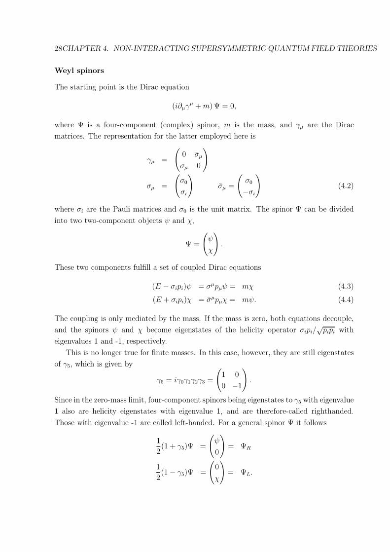
Weyl spinors
The starting point is the Dirac equation
(i∂µγµ +m) Ψ = 0,
where Ψ is a four-component (complex) spinor, m is the mass, and γµ are the Dirac
matrices. The representation for the latter employed here is
γµ =
(
0 σµ
σµ 0
)
σµ =
(
σ0
σi
)
σµ =
(
σ0
−σi
)
(4.2)
where σi are the Pauli matrices and σ0 is the unit matrix. The spinor Ψ can be divided
into two two-component objects ψ and χ,
Ψ =
(
ψ
χ
)
.
These two components fulfill a set of coupled Dirac equations
(E − σipi)ψ = σµpµψ = mχ (4.3)
(E + σipi)χ = σµpµχ = mψ. (4.4)
The coupling is only mediated by the mass. If the mass is zero, both equations decouple,
and the spinors ψ and χ become eigenstates of the helicity operator σipi/√pipi with
eigenvalues 1 and -1, respectively.
This is no longer true for finite masses. In this case, however, they are still eigenstates
of γ5, which is given by
γ5 = iγ0γ1γ2γ3 =
(
1 0
0 −1
)
.
Since in the zero-mass limit, four-component spinors being eigenstates to γ5 with eigenvalue
1 also are helicity eigenstates with eigenvalue 1, and are therefore-called righthanded.
Those with eigenvalue -1 are called left-handed. For a general spinor Ψ it follows
1
2(1 + γ5)Ψ =
(
ψ
0
)
= ΨR
1
2(1 − γ5)Ψ =
(
0
χ
)
= ΨL.

4.1. FERMIONS 29
The importance of the subspinors ψ and χ is that they have a definite behavior under
Lorentz transformations. These are therefore called Weyl spinors. To see this, take an
infinitesimal Lorentz transformation
E → E ′ = E − ηipi
p→ p′ = p− ǫ× p− ηE,
where ǫ parametrize a rotation and η a boost. With the general transformation behavior
of Dirac spinors under Lorentz transformations
Ψ′ = Ψ +i
2
(
ǫiσi − ηiσi 0
0 ǫiσi + ηiσi
)
Ψ (4.5)
the transformation rules
ψ → ψ′ = ψ + (iǫiσi/2 − ηiσi/2)ψ
χ→ χ′ = χ+ (iǫiσi/2 + ηiσi/2)χ
results. The important observation is that both transform the same under rotations, as
spin 1/2 particles, but differently under boosts. Defining
V = 1 + iǫiσi/2 − ηiσi/2
The transformation rules then simplify to
ψ′ = V ψ
χ′ = V −1+χ = (1 + iǫiσi/2 − ηiσi/2)−1+χ
= (1 − iǫiσi/2 + ηiσi/2)+χ = (1 + iǫiσi/2 + ηiσi/2)χ.
Furthermore, from equations (4.3) and (4.4) it follows then that a multiplication with σµpµ
exchanges (up to a factor m) a ψ- and a χ-type-spinor, and thus changes the respective
transformation properties under Lorentz transformations.
This is already important: Because the aim is to construct a Lorentz scalar for the
supersymmetry transformation (4.1) and to do this with only two degrees of freedom, it
is necessary to form a scalar out of Weyl spinors. For a Dirac spinor this is simple,
Ψ+γ0Ψ =(
ψ+ χ+)
(
0 1
1 0
)(
ψ
χ
)
= ψ+χ+ χ+ψ,
and thus scalars are products of ψ- and χ-type spinors. So there is already one possibility
to construct a ψ from a χ, but this involves the Dirac equation and a momentum. A more
general possibility is
σ2ψ∗′ = σ2V
∗ψ∗ = σ2(1 − iǫiσi∗/2 − ηiσ
i∗/2)ψ∗ = (1 + iǫiσi/2 + ηiσ
i/2)σ2χ = V −1+σ2ψ∗,
30CHAPTER 4. NON-INTERACTING SUPERSYMMETRIC QUANTUM FIELD THEORIES
where in the last step it was used that σ2 anti-commutes with the real σ1 and σ3 matrices,
but commutes with itself and is itself purely imaginary. Hence σ2cc →, which may be
recognized as the charge-conjugation operator, turns the Weyl-spinor ψ into one of χ-
type, with the corresponding changed Lorentz-transformation. Hence, e. g., the quantity
(−iσ2ψ∗)+ψ = (−iσ2ψ)Tψ = ψT (iσ2)ψ
is a scalar, just as desired. Similar iσ2χ∗ transforms like a ψ, and so on. Hence transfor-
mations rules can be introduced, and corresponding translations.
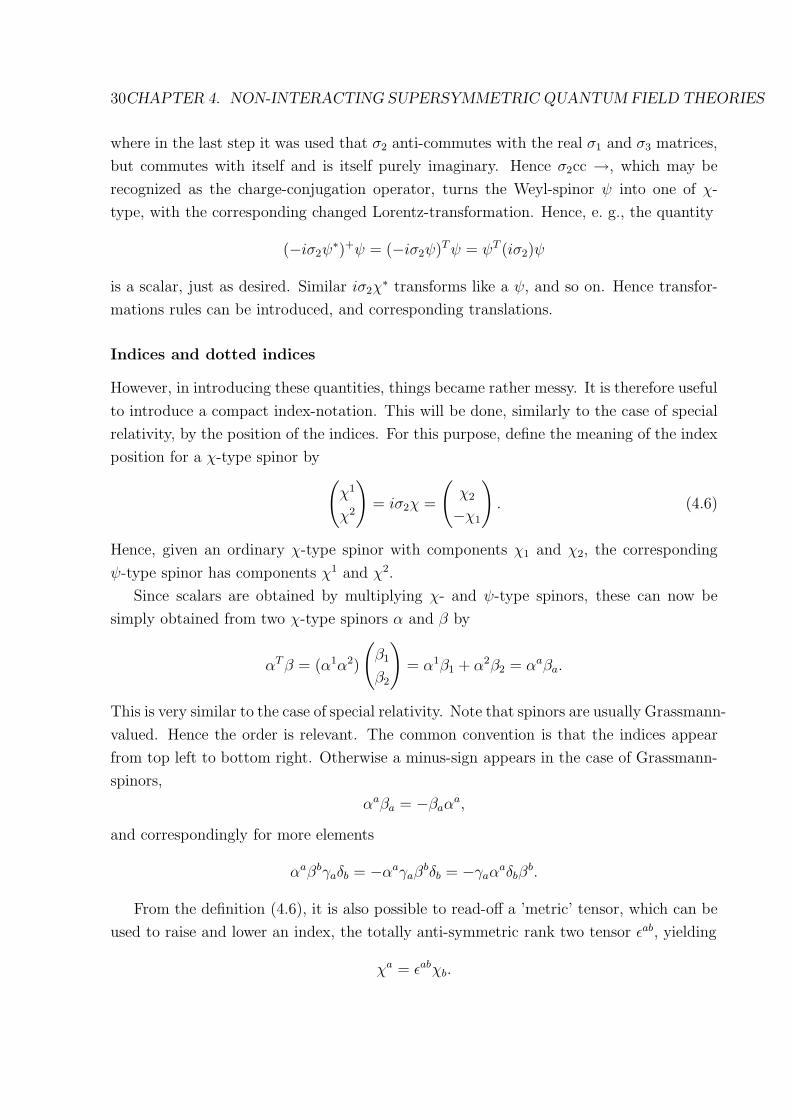
Indices and dotted indices
However, in introducing these quantities, things became rather messy. It is therefore useful
to introduce a compact index-notation. This will be done, similarly to the case of special
relativity, by the position of the indices. For this purpose, define the meaning of the index
position for a χ-type spinor by(
χ1
χ2
)
= iσ2χ =
(
χ2
−χ1
)
. (4.6)
Hence, given an ordinary χ-type spinor with components χ1 and χ2, the corresponding
ψ-type spinor has components χ1 and χ2.
Since scalars are obtained by multiplying χ- and ψ-type spinors, these can now be
simply obtained from two χ-type spinors α and β by
αTβ = (α1α2)
(
β1
β2
)
= α1β1 + α2β2 = αaβa.
This is very similar to the case of special relativity. Note that spinors are usually Grassmann-
valued. Hence the order is relevant. The common convention is that the indices appear
from top left to bottom right. Otherwise a minus-sign appears in the case of Grassmann-
spinors,
αaβa = −βaαa,
and correspondingly for more elements
αaβbγaδb = −αaγaβbδb = −γaα
aδbβb.
From the definition (4.6), it is also possible to read-off a ’metric’ tensor, which can be
used to raise and lower an index, the totally anti-symmetric rank two tensor ǫab, yielding
χa = ǫabχb.
4.1. FERMIONS 31
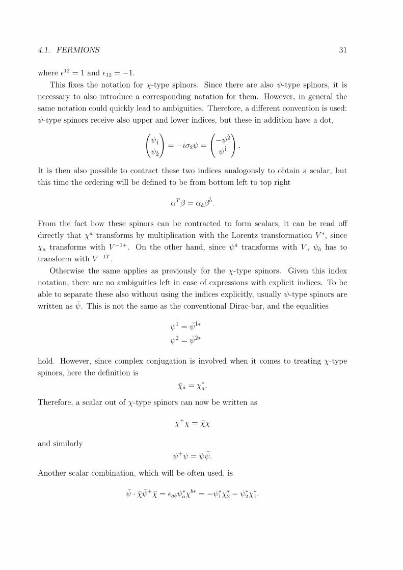
where ǫ12 = 1 and ǫ12 = −1.
This fixes the notation for χ-type spinors. Since there are also ψ-type spinors, it is
necessary to also introduce a corresponding notation for them. However, in general the
same notation could quickly lead to ambiguities. Therefore, a different convention is used:
ψ-type spinors receive also upper and lower indices, but these in addition have a dot,
(
ψ1
ψ2
)
= −iσ2ψ =
(
−ψ2
ψ1
)
.
It is then also possible to contract these two indices analogously to obtain a scalar, but
this time the ordering will be defined to be from bottom left to top right
αTβ = αaβb.
From the fact how these spinors can be contracted to form scalars, it can be read off
directly that χa transforms by multiplication with the Lorentz transformation V ∗, since
χa transforms with V −1+. On the other hand, since ψa transforms with V , ψa has to
transform with V −1T .
Otherwise the same applies as previously for the χ-type spinors. Given this index
notation, there are no ambiguities left in case of expressions with explicit indices. To be
able to separate these also without using the indices explicitly, usually ψ-type spinors are
written as ψ. This is not the same as the conventional Dirac-bar, and the equalities
ψ1 = ψ1∗
ψ2 = ψ2∗
hold. However, since complex conjugation is involved when it comes to treating χ-type
spinors, here the definition is
χa = χ∗a.
Therefore, a scalar out of χ-type spinors can now be written as
χ+χ = χχ
and similarly
ψ+ψ = ψψ.
Another scalar combination, which will be often used, is
ψ · χψ+χ = ǫabψ∗aχ
b∗ = −ψ∗1χ
∗2 − ψ∗
2χ∗1.

32CHAPTER 4. NON-INTERACTING SUPERSYMMETRIC QUANTUM FIELD THEORIES
Having now available a transformation which makes from an electron-type half spinor
a positron-like half-spinor, it is natural to investigate what happens if both are combined
into one single 4-component spinor, i. e., combining two Weyl spinor. To obtain the correct
transformation properties under Lorentz transformation, this object is
Ψ =
ψ1
ψ2
−ψ2∗
ψ1∗
.
Since there are only two independent degrees of freedom, the spinor Ψ cannot describe, e.
g., an electron. Its physical content is made manifest by performing a charge conjugation
CΨ =
(
0 iσ2
−iσ2 0
)(
ψ∗
−iσ2ψ
)
=
(
ψ
−iσ2ψ∗
)
= Ψ,
i. e., it is invariant under charge conjugation and thus describes a particle which is its own
antiparticle, like the photon. Spin 1/2-particles with this property are called Majorana
fermions.
4.2 The simplest supersymmetric theory
This is sufficient to set the scene for a first supersymmetric quantum field theory.
As discussed previously, it will be necessary to have the same number of fermionic
and bosonic degrees of freedom. This requires at least two degrees of freedom, since it
is not possible to construct a fermion with only one. Consequently, two scalar degrees of
freedom are necessary. The simplest system with this number of degrees of freedom is a
non-interacting system of a complex scalar field φ and a free Weyl fermion χ, which will
be described by the undotted spinor. The corresponding Lagrangian is given by
L = ∂µφ+∂µφ+ iχ+σµ∂µχ. (4.7)
Note that here already with the fully quantized theory will be dealt. From this the
corresponding action is constructed as
S =
∫
Ld4x.
The corresponding physics will be invariant under a supersymmetry transformation
if the action is invariant1. Since it is assumed that the fields vanish at infinity this re-
1Actually, only up to anomalies. This possibility will be disregarded here, and is no problem for the
cases presented.

4.2. THE SIMPLEST SUPERSYMMETRIC THEORY 33
quires invariance of the Lagrangian under the supersymmetry transformation up to a total
derivative.
The according supersymmetry transformation can be constructed by trial and error.
Here, they will be introduced with hindsight of the results, and afterwards their properties
will be analyzed. The transformation
A′ = A+ δA
takes for the scalar field the form
δφ = ξaχa = (−iσ2ξ)Tχ. (4.8)
Herein, ξ is a constant, Grassmann-valued spinor. It thus anticommutes with χa. This is
necessary in order to form a scalar, complex number from χ. By dimensional analysis, ξ
has units of 1/√
mass. The corresponding transformation law for the spinor is
δχ = −iσµξ∂µφ = σµσ2ξ∗∂µφ. (4.9)
The pre-factor is fixed by the requirement that the Lagrangian is invariant under the
transformation. The combination of ξ with σµ guarantees the correct transformation
behavior of the expression under Lorentz transformation in spinor space. The derivative,
which appears then, is then necessary to construct a scalar under Lorentz transformation
in space-time, and to obtain the correct mass-dimension. It is the only object which can be
used for this purposes, as it is the only one which appears in the Lagrangian (4.7), besides
the scalar field. The general structure is therefore fixed by the transformation properties
under Lorentz transformation. That the pre-factors are in fact also correct can be shown
by explicit calculation,
δL = ∂µ((δφ)+)∂µφ+ ∂µφ+∂µ(δφ) + (δχ)+iσµ∂µχ+ χ+iσµ∂µ(δχ)
= i∂µχ+σ2ξ
∗∂µφ+ iχ+σνσµσ2ξ∗∂ν∂µφ− i∂µφ
+∂µ(ξTσ2χ) − iξTσ2σµσνχ∂ν∂µφ
+(4.10)
Herein partial integrations have been performed, as necessary to obtain this form. There
are two linearly independent terms, one proportional to ξ∗ and one to ξ in this expression.
Both have therefore to either individually vanish or be total derivatives. To show this, it
is helpful to note that
σν∂νσµ∂µ = (∂0 − σj∂j)(∂
0 + σi∂i) = ∂0∂
0 − ∂i∂i = ∂µ∂µ, (4.11)
where it has been used that σ2i = 1. Taking now only the terms proportional to ξ∗ yields
i∂µχ+σ2ξ
∗∂µφ+ iχ+σ2ξ∗∂µ∂
µφ = ∂µ(χ+iσ2ξ∗∂µφ). (4.12)
34CHAPTER 4. NON-INTERACTING SUPERSYMMETRIC QUANTUM FIELD THEORIES
This term is therefore indeed a total derivative. Likewise, also the term proportional ξT
can be manipulated to yield a pure total derivative. However, this is somewhat more
complicated, as the combination (4.11) is not appearing. The last term can be rewritten
as
−iξTσ2σµσνχ∂ν∂µφ
+ = ∂µ(φ+iξTσ2σµσν∂νχ) + φ+iξTσ2σ
µσν∂µ∂νχ
It is then possible to use (4.11) on the last term to obtain
∂µ(φ+iξTσ2σν σµ∂νχ) + φ+iξTσ2∂µ∂µχ.
The first term is already a total derivative. The second term combines with the second-to-
last term of (4.10) to a total derivative. Hence, the total transformation of the Lagrangian
reads
δL = ∂µ(χ+iσ2ξ∗∂µφ+ φ+iξTσ2σ
ν σµ∂νχ+ φ+iξTσ2∂µχ)
which is a total derivative.
Therefore, this theory is indeed supersymmetric. The set of fields φ and χ is called a
super-multiplet. To be more precise, it is a left chiral super-multiplet, because the spinor
has been taken to be of χ-type. The χ-type spinor could be replaced with a ψ-type spinor,
yielding a right chiral multiplet, without changing the supersymmetry of theory, although,
of course, the transformation is modified.
There should be a note of caution here. Unfortunately, it will turn out that this
demonstration is insufficient to show supersymmetry of the quantized theory, and it will
be necessary to modify the Lagrangian (4.7). This problem will become apparent when
discussing the supersymmetry algebra. However, most of the calculations performed so
far can be used unchanged.
4.3 Supersymmetry algebra
It turns out that the supersymmetry transformations (4.8) and (4.9) will form an alge-
bra, similar to the algebra (2.9) of the quantum mechanical case. This algebra can be
used to systematically construct supermultiplets, and is useful for many other purposes.
Therefore, this algebra will be constructed here, based first on the simplest examples of
supersymmetry transformations (4.8) and (4.9) and will be generalized thereafter.
4.3.1 Constructing an algebra from a symmetry transformation
Such an algebra has already been encountered in the quantum mechanical case, and was
given by (2.9). To obtain this algebra, it is necessary to construct the supersymmetry

4.3. SUPERSYMMETRY ALGEBRA 35
charges, which in turn generate the transformation. This is constructed as follows. In
general, any symmetry transformation is an unitary transformation to preserve observ-
ables. Thus for any field f , in general a transformation can be written as
f ′ = UfU+ (4.13)
with U an unitary operator. Any unitary operator can be written as
U = exp(iξQ)
with Q hermitian, Q = Q+. If the transformation parameter ξ becomes infinitesimal, the
relation (4.13) can be expanded to yield
f ′ = (1 + iξQ)f(1 − iξQ) = f + [iξQ, f ].
δf = [iξQ, f ].
In a quantum field theory, Q must be again a function of the f . To construct it, it is nec-
essary to analyze the transformation properties of the Lagrangian under the infinitesimal
transformation, which is given by
δL = ∂µKµ (4.14)
The terms on the right-hand side are total derivatives, which may appear. For simplicity,
it will be assumed that the transformation U is not inducing such terms, but it will be
necessary to include them below when returning to supersymmetry transformations, as
there such terms are present, see (4.12). If then ∂K is dropped, the variation can be
written as
0 = δL =∂L∂f
δf +∂L∂∂µf
∂µ(δf).
This can be simplified using the equation of motion for f ,
∂L∂f
= ∂µ
(
∂L∂∂µf
)
to yield
0 =
(
∂µ
(
∂L∂∂µf
))
δf +∂L∂∂µf
∂µ(δf) = ∂µ
(
∂L∂∂µf
δf
)
= ∂µjµ. (4.15)
The current which has been thus defined is the symmetry current, and it is conserved. If
a total derivative ∂µKµ exists, the definition of the symmetry current becomes
jµ =∂L∂∂µf
δf −Kµ (4.16)

36CHAPTER 4. NON-INTERACTING SUPERSYMMETRIC QUANTUM FIELD THEORIES
Therefore, the charge defined as
q =
∫
ddxj0(x)
is also conserved. This derivation is also known as Noethers theorem, stating that for any
symmetry there exists a conserved charge. Note that this charge is an operator, build from
the field variables. It can be identified with the charge Q, which in general can be shown
by an expansion of its constituents in power-series in f and ∂µf (ensuring the invariance
of L) and the usage of the commutation relations of f . This will not been done here, but
below an explicit examples for the case of supersymmetry will be discussed.
This completed, and thus with an explicit expression for generators of the transfor-
mation Q at hand, it is possible to construct the corresponding algebra by evaluating the
(anti-)commutators of Q.
4.3.2 The superalgebra
The conserved supercurrent jµ can be constructed using (4.14) and (4.15). Noting that
∂µχ+ is not appearing in the Lagrange density, only three derivatives plus the boundary
term remain to yield
jµ = −Kµ +∂L∂∂µφ
δφ+∂L
∂∂µφ+δφ+ +
∂L∂∂µχ
δχ
= −χ+iσ2ξ∗∂µφ+ ∂νφ
+iξTσ2σν σµχ + φ−iξTσ2∂µχ
−∂µφ+ξT iσ2χ+ χ+iσ2ξ∗∂µφ+ χ+σµσνiσ2ξ
∗∂νφ
Here, and in the following, the necessary contribution from the hermitiean conjugate
contribution are not marked explicitly. This can be directly reduced, since some terms
cancel, to
jµ = χ+σµσνiσ2ξ∗∂νφ− ∂νφ
+iξTσ2σν σµχ
= ξT (−iσ2)Jµ + ξ∗iσ2J
µ∗
Jµ = σν σµχ∂νφ+.
Jµ is the so-called super-current, which forms the conserved current by a hermitian combi-
nation, similar to the probability current in ordinary quantum mechanics, iψ+∂iψ+iψ∂iψ+.
To write the complex-conjugate part of the current, it has been used that
σ2σν σµ = σν σµσ2

4.3. SUPERSYMMETRY ALGEBRA 37
which follows by the anti-commutation rules for the Pauli matrices. This permits to
construct the supercharge
Q =
∫
d3xσνχ∂νφ+.
These indeed generate the transformation for the fields φ and χ. To show this, the canon-
ical commutation relations
[φ(x, t), ∂tφ(y, t)] = iδ(x− y)
{χa(x, t), χ+b (y, t)} = δabδ(x− y), (4.17)
and all other (anti-)commutators vanishing, are necessary.
For the bosonic fields this follows as
i[ξQ, φ(x)] = i
∫
dy[ξ(σνχ(y))∂νφ+(y), φ(x)]
= i
∫
dyξσνχ(y)[∂νφ+(y), φ(x)] (4.18)
Since the commutator of all spatial derivatives with the field itself vanishes, only the
component ν = 0 remains,
i
∫
dyξχ(y)[∂0φ+(y), φ(x)] =
∫
dyξχ(y)δ(x− y) = ξχ
which is exactly the form (4.8). The calculation for the transformation of φ+ has to be
performed with ξQ, and yields the transformation rule for χ. Consequently, the transfor-
mation law for χ is obtained from
i[ξQ+ ξQ, χ(x)] = −iσµ(iσ2ξ∗)∂µφ,
and correspondingly for χ+ from the complex conjugate version. To explicitly show this,
it is necessary to note that
[ξaχ+a, χb] = ξaχ
+aχb − χbξaχa = ξaχ
+aχb + ξaχbχa = ξa{χ+a, χb},
since Grassmann fields and variables anticommute.
Now it is possible to construct the algebra.
First of all, the (anti-)commutators
[Q, Q] = 0 [Q,Q] = 0 {Q,Q} = 0 {Q, Q} = 0
all vanish, since in all cases all appearing fields (anti-)commute. There are thus, at first
sight, one non-trivial commutator and one non-trivial anti-commutator.
38CHAPTER 4. NON-INTERACTING SUPERSYMMETRIC QUANTUM FIELD THEORIES
For the non-vanishing cases, it is more simply to evaluate two consecutive applications
of SUSY transformations. To perform this, note first that
[q, [p, f ]] + [p, [f, q]] + [f, [q, p]] = 0.
This can be shown by direct expansion. It can be rearranged to yield
[[q, p], f ] = [q, [p, f ]] − [p, [q, f ]].
If q and p are taken to be ξQ and ηQ, and f taken to be φ, this implies that the commutator
of two charges can be obtained by determining the result from two consecutive applications
of the SUSY transformations. Using (4.8) and (4.9), it is first possible to obtain the result
for this double application. It takes the form
[ξQ+ ξQ, [ηQ+ ηQ, φ]] = −i[ξQ+ ξQ, ηT (−iσ2)χ] = iηT (−iσ2)σµ(−iσ2ξ
∗)∂µφ. (4.19)
Subtracting both possible orders of application yields then the action of the commutator
[[ξQ+ ξQ, ηQ+ ηQ], φ] = i(ξT (−iσ2)σµ(−iσ2η
∗) − ηT (−iσ2)σµ(−iσ2ξ
∗))∂µφ.
Here it has been used that Q is commuting with φ, as it does not depend on φ+.
Aside from a lengthy expression, which gives the composition rule for the parameters,
there is one remarkable result: The appearance of −i∂µφ, which is the action of Pµ on φ,
the momentum or generator of translations. Hence, the commutator is given by
[ξQ+ ξQ, ηQ+ ηQ, φ] = f(η, ξ)Pµ. (4.20)
In fact, this is not all, due to aforementioned subtlety involving the fermions. This will be
postponed to later. The appearance of the momentum operator seems at first surprising.
However, in quantum mechanics it has been seen that the super-charges are something like
the squareroot of the Hamilton operator, which is also applying, in the free case, to the
momentum operator. This relation is hence less exotic than might be anticipated. Still,
this implies that the supercharges are also something like the squareroot of the momen-
tum operator, which lead to the notion of the supercharge being translation operators in
fermionic dimensions. This idea will be taken up later when the superspace formulation
will be discussed. Another important sideremark is that this result implies that making
supersymmetry a local gauge symmetry this connection yields automatically a connection
to general relativity, the so-called supergravity theories. This is, unfortunately, far beyond
the scope of the current lecture.
Hence, the algebra for the SUSY-charges will not only contain the charges themselves,
but necessarily also the momentum operator. However, the relations are rather simple, as
4.3. SUPERSYMMETRY ALGEBRA 39
the supercharges do not depend on space-time and thus (anti-)commute with the momen-
tum operator, as does the latter with itself.
Thus, the remaining item is the anticommutator of Q with Q. For this, again the
commutator is useful, as it can be expanded as
[ηQ, ξQ+] = η1ξ∗1(Q2Q
+2 +Q+
2 Q2) − η1ξ∗2(Q2Q
+1 +Q+
1 Q2)
−η2ξ∗1(Q1Q
+2 +Q+
2 Q1) + η2ξ∗2(Q1Q
+1 +Q+
1 Q1)
Thus, all possible anticommutators appear in this expression. The explicit expansion of
(4.20) is
(η2ξ∗2(σµ)11 − η2ξ
∗1(σµ)12 − η1ξ
∗2(σµ)21 + η1ξ
∗1(σµ)22)P
µ.
Thus, by coefficient comparison the anticommutator is directly obtained as
{Qa, Q+b } = (σµ)abPµ. (4.21)
This completes the algebra for the supercharges, which is in the field-theoretical case
somewhat more complicated by the appearance of the generator of translations, but also
much richer.
There are two remarks in order.
First, again, a subtlety will require to return to these results shortly.
Secondly, this results looks somewhat different from the quantum mechanical case (2.9),
where there have been two supercharges, instead of one, which then did not anticommute
as is the case here. Also in field theories this may happen, if there are more than one
supercharge. Since in the case of multiple supercharges there is still only one momentum
operator, the corresponding superalgebras are coupled. In genereal, this requires the
introduction of another factor δAB, where A and B count the supercharges. It appears
in the (anti-)commutator of QA with QB. The more drastic change is, however, that the
anticommutator becomes modified to
{QAa , Q
Bb } = ǫabZ
AB,
and correspondingly for QA and QB. The symbol ǫab is anti-symmetric, and thus this
anticommutator couples the algebra of different supercharges. Furthermore, the ZAB are
called the central charges, and are also anti-symmetric, but not an operator. The number
of independent supercharges is labeled by N . The theory with only one supercharge is
thus an N = 1 theory. In four dimensions, there are also N = 2 and N = 4 theories. The
additional charges provide more constraints, so theories with more supercharges become
easier to handle. However, currently there seems to exist no hint that any other than

40CHAPTER 4. NON-INTERACTING SUPERSYMMETRIC QUANTUM FIELD THEORIES
N = 1-theories could be realized at energy scales accessible in the foreseeable future.
Thus, here only this case will be treated, and the remaining theories are beyond the scope
of this lecture.
4.3.3 Supermultiplets
A supermultiplet is a collection of fields which transform into each other under supersym-
metry transformations. The naming convention is that a fermionic superpartner of a field a
is called a-ino,and a bosonic superpartner s-a. Here, the structure of these supermultiplets
will be analyzed.
One result of the algebra obtained in the previous subsection was that the momentum
operator (anti-)commutes with all supercharges. Consequently, also P 2 (anti-)commutes
with all supercharges,
[Qa, P2] = [Q, P 2] = {Q,P 2} = {Q, P 2} = 0.
Since the application of P 2 just yields the mass of a pure state, the masses of a particle s
and its superpartner ss must be degenerate, symbolically
P 2|s > = m2|s >P 2|ss > = P 2Q|s >= QP 2|s >= Qm2|s >= m2Q|s >= m2|ss > .
This is very similar to the degenerate energy levels, which were encountered in the quantum
mechanical case.
Further insight can be gained from considering the general pattern of the angular
momentum in a supermultiplet. So far, it is only clear that in a supermultiplet bosons
and fermions must be present, but not necessarily their spin. In the example, one was a
spin-0 particle and one a spin-1/2 particle. This pattern of a difference in spin of 1/2 is
general.
This can be seen by considering the commutation relations of the supercharges under
rotation. Since the supercharges are spinors, they must behave under a rotation δǫ as
δǫQ = −iǫσ2Q = iǫ[J,Q],
where J is the generator of rotations. In particular, for the third component follows
[J3, Q] = −1
2σ3Q
and thus
[J3, Q1] = −1
2Q1 [J3, Q2] =
1
2Q2 (4.22)
4.3. SUPERSYMMETRY ALGEBRA 41
for both components of the spinor Q. It then follows directly that the superpartner of
a state with total angular momentum j and third component m has third component
m± 1/2, depending on the transformed spinor component. This can be seen as
J3Q1|jm >= (Q1J3 − [Q1, J3])|jm >=
(
Q1m− 1
2Q1
)
|jm >= Q1
(
m− 1
2
)
|jm > .
Likewise, the other spinor component of Q yields the other sign, and thus raises instead of
lowers the third component. Of course, this applies vice-versa for the hermitian conjugates.
To also determine the value of j, assume a massless state with momentum (p,0,0,p).
The massive case is analogous, but more tedious. Start with the lowest state with m = −j.Then, of course, the state is annihilated by Q1 and Q+
2 , as they would lower m further.
Also Q+1 annihilates the state, which is a more subtle result. The anticommutator
yields the result
Q+1 Q1 +Q1Q
+1 = (σµ)11P
µ = P 0 − P 3,
where the minus-sign in the second term appears due to the metric. Thus
< pj − j|Q+1 Q1 +Q1Q
+1 |pj − j >= p0 − p3 = p− p = 0 (4.23)
but also
< pj − j|Q+1 = (Q1|pj − j >)+ = 0,
as discussed above. Hence the first term in (4.23) vanishes, and leaves
< pj − j|Q1Q+1 |pj − j >= 0.
But this is just the norm of Q+1 |pj − j >. A zero-norm state is however not appropriate
to represent a particle state2, and thus Q+1 has to annihilate the state as well, the only
alternative to obtain the same result.
This leaves only Q2|pj − j > as a non-zero state. This state has to be proportional to
a state of type |pj− j+ 1/2 >. Since Q2 is Grassmann-valued, and therefore nil-potent, a
second application of Q2 yields again zero. Furthermore, since Q1 and Q2 anticommute,
its application also yields zero,
Q1Q2|pj − j >= −Q2Q1|pj − j >= 0.
The application of Q+1 can be calculated as in the case of (4.23). But the appearing
momentum combination is P1+P2, being zero for the state. This leaves only Q+2 . Applying
it yields
Q+2 Q2|pj − j >= ((σµ)22P
µ −Q2Q+2 )|pj − j >= (p0 + p3 + 0)|pj − j >= 2p|pj − j > .
2In gauge theories, this statement has to be refined.

42CHAPTER 4. NON-INTERACTING SUPERSYMMETRIC QUANTUM FIELD THEORIES
Hence, this return the original state. Thus, the value of j in a supermultiplet can differ
only by two, and there are only two (times the number of internal quantum number) states
in each supermultiplet. It does not specify the value of j, so it would be possible to have
a supermultiplet with j = 0 and j = 1/2, as in the example above. Note that only the
states m = 0 and m = −1/2, but not m = +1/2, the anti-particle state are contained in
the supermultiplet. This is called a chiral multiplet. Alternatively, it would be possible to
have j = 1/2 and j = 1, the vectormultiplet, or j = 1 and j = 3/2, the gravity multiplet
appearing in supergravity.
However, any quantum field theory has the CPT-symmetry, thus for any supermultiplet
also its CPT-transformed supermultiplet, and thus the corresponding antiparticles, have
also to appear in the theory as well. By this, the missing m = 1/2 state above is introduced
into the theory.
Note that here the absence of central charges was important, since the anticommutator
of the fields has been used. In theories with more supercharges, the supermultiplets become
larger. E.g. in N = 2 SUSY, the supermultiplet contains two states with j = 0 and two
with m = ±1/2. This is also the reason why theories with N 6= 1 seem to be no good
candidates for an extension of the standard model: SUSY, as will be seen below, requires
that all superpartners transform the same under other transformations, like e. g. gauge
transformations. In an N = 2 theory, there would be a left-handed and a right-handed
electron, both transforming under all symmetries in the same way. But in the standard
model, the weak interactions couple differently to left-handed and right-handed electrons,
and thus it is not compatible with N > 1 SUSY. For N = 1 SUSY, however, independent
chiral multiplets (and, thus, more particles) can be introduced solving this problem. Since
also the quarks (and the superpartners of the gauge-bosons therefore should also) are
coupled differently in the weak interactions, this applies to all matter-fields, and thus it is
not possible to enhance some particles with N = 1 and others with N > 1 SUSY.
4.3.4 Off-shell supersymmetry
Now, it turns out that the results so far are not complete. If in (4.19) instead of φ the
superpartner χ is used, it turns out that complications arise. Thus, something has to be
modified.
To see this inconsistency, start by first performing two supersymmetry transformation
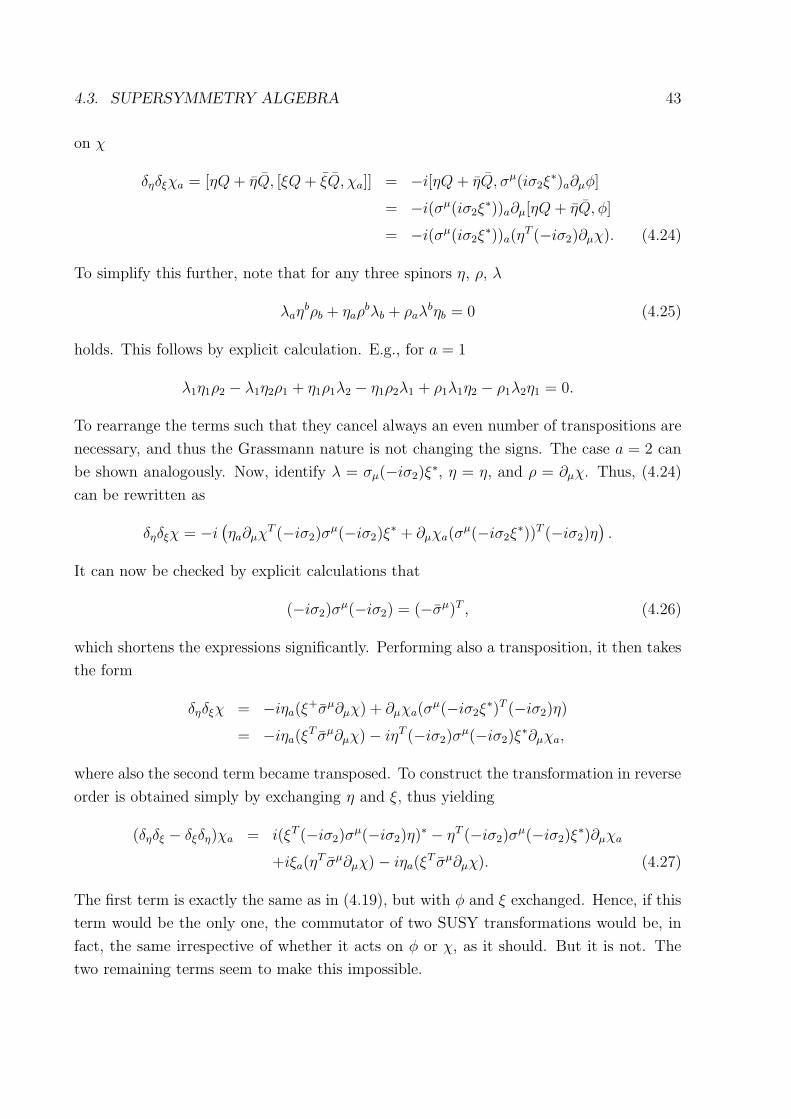
4.3. SUPERSYMMETRY ALGEBRA 43
on χ
δηδξχa = [ηQ+ ηQ, [ξQ+ ξQ, χa]] = −i[ηQ+ ηQ, σµ(iσ2ξ∗)a∂µφ]
= −i(σµ(iσ2ξ∗))a∂µ[ηQ+ ηQ, φ]
= −i(σµ(iσ2ξ∗))a(η
T (−iσ2)∂µχ). (4.24)
To simplify this further, note that for any three spinors η, ρ, λ
λaηbρb + ηaρ
bλb + ρaλbηb = 0 (4.25)
holds. This follows by explicit calculation. E.g., for a = 1
λ1η1ρ2 − λ1η2ρ1 + η1ρ1λ2 − η1ρ2λ1 + ρ1λ1η2 − ρ1λ2η1 = 0.
To rearrange the terms such that they cancel always an even number of transpositions are
necessary, and thus the Grassmann nature is not changing the signs. The case a = 2 can
be shown analogously. Now, identify λ = σµ(−iσ2)ξ∗, η = η, and ρ = ∂µχ. Thus, (4.24)
can be rewritten as
δηδξχ = −i(
ηa∂µχT (−iσ2)σ
µ(−iσ2)ξ∗ + ∂µχa(σ
µ(−iσ2ξ∗))T (−iσ2)η
)
.
It can now be checked by explicit calculations that
(−iσ2)σµ(−iσ2) = (−σµ)T , (4.26)
which shortens the expressions significantly. Performing also a transposition, it then takes
the form
δηδξχ = −iηa(ξ+σµ∂µχ) + ∂µχa(σ
µ(−iσ2ξ∗)T (−iσ2)η)
= −iηa(ξT σµ∂µχ) − iηT (−iσ2)σ
µ(−iσ2)ξ∗∂µχa,
where also the second term became transposed. To construct the transformation in reverse
order is obtained simply by exchanging η and ξ, thus yielding
(δηδξ − δξδη)χa = i(ξT (−iσ2)σµ(−iσ2)η)
∗ − ηT (−iσ2)σµ(−iσ2)ξ
∗)∂µχa
+iξa(ηT σµ∂µχ) − iηa(ξ
T σµ∂µχ). (4.27)
The first term is exactly the same as in (4.19), but with φ and ξ exchanged. Hence, if this
term would be the only one, the commutator of two SUSY transformations would be, in
fact, the same irrespective of whether it acts on φ or χ, as it should. But it is not. The
two remaining terms seem to make this impossible.

44CHAPTER 4. NON-INTERACTING SUPERSYMMETRIC QUANTUM FIELD THEORIES
However, on closer inspection it becomes apparent that in both terms the expression
σµ∂µχ exists. This is precisely the equation of motion for the field χ, the Weyl equation.
Thus the two terms vanish, if the field satisfies its equation of motion. In a classical
theory, this would be sufficient. However, in a quantum theory exist virtual particles, i. e.,
particles which not only not fulfill the energy conservation, but also not their equations of
motions. Hence such particles, which are called off (mass-)shell are necessary. Thus the
algebra so far is said to close only on-shell. Hence, although the theory described by the
Lagrangian (4.7) is classically supersymmetric, but not so quantum-mechanical. Quantum
effects break the supersymmetry of this model.
Hence, it is necessary to modify (4.7), to change the theory, to obtain one which is also
supersymmetric on the quantum level. Actually, this result is already an indication of how
this can be done. Off-shell, the number of degrees of freedom for a Weyl-fermion is four,
and not two, as there are two complex functions, one for each spinor component. Thus,
the theory cannot be supersymmetric off-shell, as the scalar field has only two degrees of
freedom. To make the theory thus supersymmetric also off-shell, more (scalar) degrees of
freedom are necessary, which, however, do not contribute at the classical level.
This can be done by the introduction of an auxiliary scalar field, which has to be
complex to provide two degrees of freedom. It is called auxiliary, as it has no consequence
for the classical theory. The later can be most simply achieved by giving no kinetic term
to this field. Thus, the modified Lagrangian takes the form
L = ∂µφ+∂µφ+ χ+iσµ∂µχ+ F+F. (4.28)
It should be noted that this field has mass-dimension two, instead of one as the other
scalar field φ. The equation of motions for this additional field is
∂µδLδ∂µF
− δLδF
= F+ = 0(= F ).
Thus, indeed, at the classical level it does not contribute.
Of course, if it should contribute at the quantum level, it cannot be invariant under a
SUSY transformation. The simplest (and correct) guess is that this transformation should
only be relevant off-shell. As it must make a connection to χ, the ansatz is
δξF = −iξ+σµ∂µχ
δξF+ = i∂µχ
+σµξ,
where ξ has been inserted as its transpose to obtain a scalar. The appearance of the
derivative is also enforced to obtain a dimensionally consistent equation.
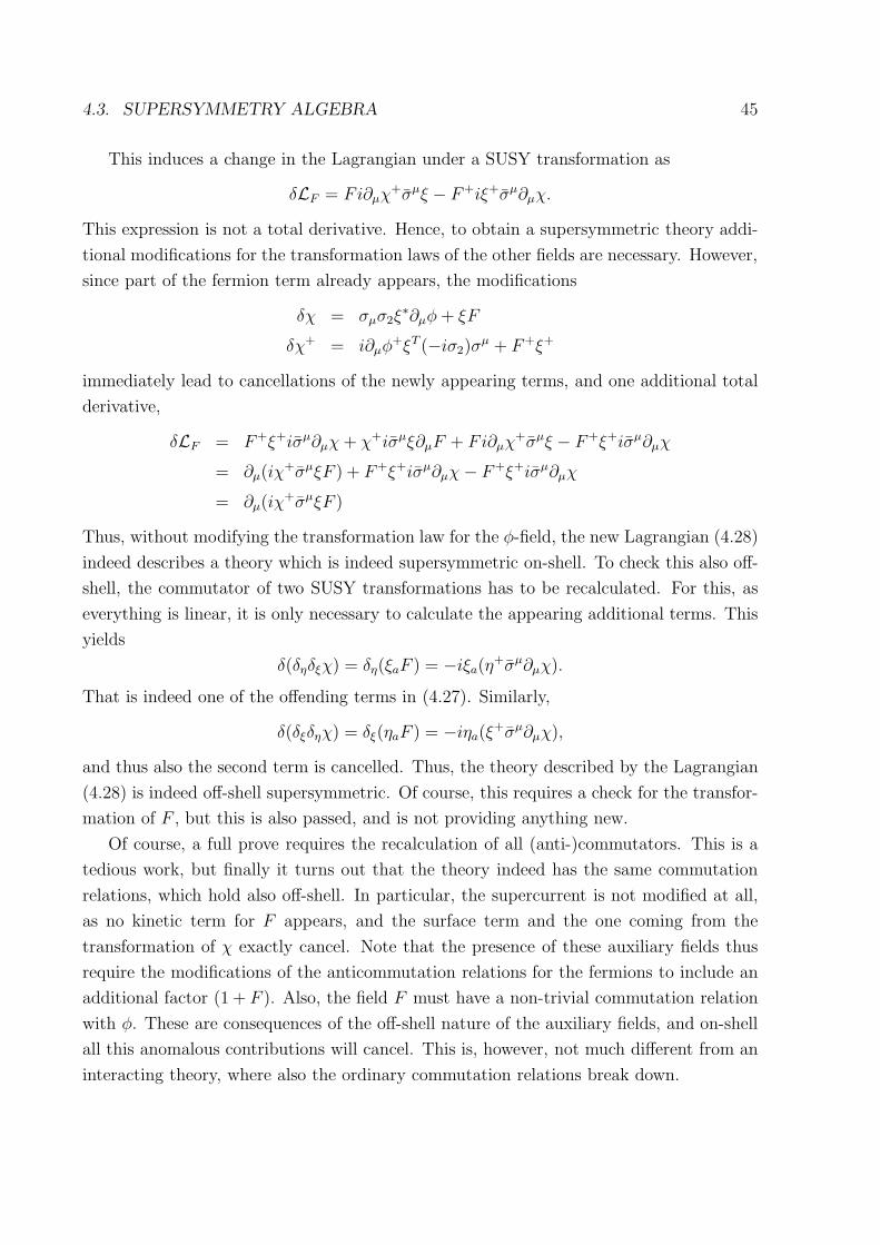
4.3. SUPERSYMMETRY ALGEBRA 45
This induces a change in the Lagrangian under a SUSY transformation as
δLF = Fi∂µχ+σµξ − F+iξ+σµ∂µχ.
This expression is not a total derivative. Hence, to obtain a supersymmetric theory addi-
tional modifications for the transformation laws of the other fields are necessary. However,
since part of the fermion term already appears, the modifications
δχ = σµσ2ξ∗∂µφ+ ξF
δχ+ = i∂µφ+ξT (−iσ2)σ
µ + F+ξ+
immediately lead to cancellations of the newly appearing terms, and one additional total
derivative,
δLF = F+ξ+iσµ∂µχ+ χ+iσµξ∂µF + Fi∂µχ+σµξ − F+ξ+iσµ∂µχ
= ∂µ(iχ+σµξF ) + F+ξ+iσµ∂µχ− F+ξ+iσµ∂µχ
= ∂µ(iχ+σµξF )
Thus, without modifying the transformation law for the φ-field, the new Lagrangian (4.28)
indeed describes a theory which is indeed supersymmetric on-shell. To check this also off-
shell, the commutator of two SUSY transformations has to be recalculated. For this, as
everything is linear, it is only necessary to calculate the appearing additional terms. This
yields
δ(δηδξχ) = δη(ξaF ) = −iξa(η+σµ∂µχ).
That is indeed one of the offending terms in (4.27). Similarly,
δ(δξδηχ) = δξ(ηaF ) = −iηa(ξ+σµ∂µχ),
and thus also the second term is cancelled. Thus, the theory described by the Lagrangian
(4.28) is indeed off-shell supersymmetric. Of course, this requires a check for the transfor-
mation of F , but this is also passed, and is not providing anything new.
Of course, a full prove requires the recalculation of all (anti-)commutators. This is a
tedious work, but finally it turns out that the theory indeed has the same commutation
relations, which hold also off-shell. In particular, the supercurrent is not modified at all,
as no kinetic term for F appears, and the surface term and the one coming from the
transformation of χ exactly cancel. Note that the presence of these auxiliary fields thus
require the modifications of the anticommutation relations for the fermions to include an
additional factor (1 + F ). Also, the field F must have a non-trivial commutation relation
with φ. These are consequences of the off-shell nature of the auxiliary fields, and on-shell
all this anomalous contributions will cancel. This is, however, not much different from an
interacting theory, where also the ordinary commutation relations break down.
Chapter 5
Interacting supersymmetric quantum
field theories
5.1 The Wess-Zumino model
The theory treated so far was non-interacting and, after integrating out F with use of its
equations of motions, had a very simple particle content. Of course, any relevant theory
should be interacting. The construction of the simplest interacting supersymmetric theory
will again be based on the Lagrangian
L = ∂µφ+∂µφ+ χ+iσµ∂µχ+ F+F + Li(φ, φ
+, χ, χ+, F, F+) + L+i .
The second term is just the hermitiean conjugate of the first term, necessary to make
the Lagrangian real. It is now necessary to find an interaction Lagrangian Li such that
supersymmetry is preserved.
Since the theory should be renormalizable, the maximum dimension (for the relevant
case of 3+1 dimensions) of the interaction terms is 4. The highest dimensional fields are
F and χ. Furthermore, the interaction terms should be scalars. Thus the possible form is
restricted to
Li = U(φ, φ+)F − 1
2V (φ, φ+)χaχa.
The −1/2 is introduced for later convenience. On dimensional grounds, with F having
dimension E2 and χ E3
2 , no other terms involving these fields are possible. In principle it
would appear possible to also have a term Z(φ, φ+), depending only on the scalar fields.
However, such a term could not include derivative terms. Under a SUSY transformation
φ is changed into χ. Hence, the SUSY transformation will yield a term with three φ
fields and one χ field for dimensional reasons, and no derivatives or F fields. However,
46
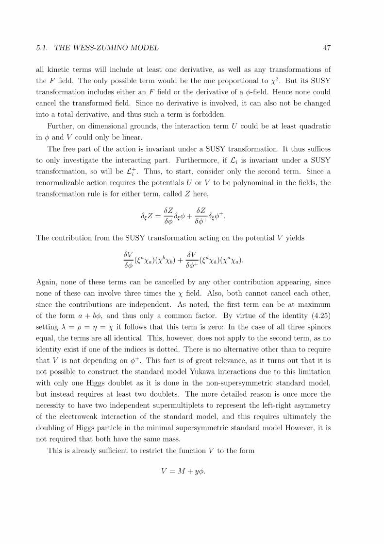
5.1. THE WESS-ZUMINO MODEL 47
all kinetic terms will include at least one derivative, as well as any transformations of
the F field. The only possible term would be the one proportional to χ2. But its SUSY
transformation includes either an F field or the derivative of a φ-field. Hence none could
cancel the transformed field. Since no derivative is involved, it can also not be changed
into a total derivative, and thus such a term is forbidden.
Further, on dimensional grounds, the interaction term U could be at least quadratic
in φ and V could only be linear.
The free part of the action is invariant under a SUSY transformation. It thus suffices
to only investigate the interacting part. Furthermore, if Li is invariant under a SUSY
transformation, so will be L+i . Thus, to start, consider only the second term. Since a
renormalizable action requires the potentials U or V to be polynominal in the fields, the
transformation rule is for either term, called Z here,
δξZ =δZ
δφδξφ+
δZ
δφ+δξφ
+.
The contribution from the SUSY transformation acting on the potential V yields
δV
δφ(ξaχa)(χ
bχb) +δV
δφ+(ξaχa)(χ
aχa).
Again, none of these terms can be cancelled by any other contribution appearing, since
none of these can involve three times the χ field. Also, both cannot cancel each other,
since the contributions are independent. As noted, the first term can be at maximum
of the form a + bφ, and thus only a common factor. By virtue of the identity (4.25)
setting λ = ρ = η = χ it follows that this term is zero: In the case of all three spinors
equal, the terms are all identical. This, however, does not apply to the second term, as no
identity exist if one of the indices is dotted. There is no alternative other than to require
that V is not depending on φ+. This fact is of great relevance, as it turns out that it is
not possible to construct the standard model Yukawa interactions due to this limitation
with only one Higgs doublet as it is done in the non-supersymmetric standard model,
but instead requires at least two doublets. The more detailed reason is once more the
necessity to have two independent supermultiplets to represent the left-right asymmetry
of the electroweak interaction of the standard model, and this requires ultimately the
doubling of Higgs particle in the minimal supersymmetric standard model However, it is
not required that both have the same mass.
This is already sufficient to restrict the function V to the form
V = M + yφ.

48CHAPTER 5. INTERACTING SUPERSYMMETRIC QUANTUM FIELD THEORIES
The first term gives a mass to the fermionic fields, and the second term provides a Yukawa
interaction. It is convenient, as will be shown latter, to write a generating functional for
this term V as
V =δW
δφδφ
with
W = B + Aφ+1
2Mφ2 +
1
6yφ3. (5.1)
This function W is called the superpotential for historically reasons, and will play a central
role, as will be seen later. The linear term is not playing a role here, but can be important
for the breaking of SUSY, as will be discussed later. The constant is essentially always
irrelevant.
The next step is to consider all terms which produce a derivative term upon a SUSY
transformation. These are
−iUξ+σµ∂µχ + i1
2V χTσ2σ
µσ2ξ∗∂µφ− i
1
2V ξ+σ2σ
µTσ2χ∂µφ
= −iUξ+σµ∂µχ− i1
2V ξ+σ2σ
µTσ2χ∂µφ− i1
2V ξ+σ2σ
µTσ2χ∂µφ
= −iUξ+σµ∂µχ− i1
2V ξ+σµχ∂µφ− i
1
2V ξ+σµχ∂µφ
= −iUξ+σµ∂µχ− iV ξ+σµχ∂µφ,
where (4.26) was used twice. The combination of derivatives of φ and χ cannot be produced
by any other contribution, since all other terms will not yield derivatives. Since neither
U nor V are vectors, there are also no possibilities for a direct cancellation of both terms.
The only alternative is thus that both terms could be combined to a total derivative. This
is possible, if
U =δW
δφ
as can be seen as follows
−iξ+σµ (U∂µχ+ χV ∂µφ)
= −iξ+σµ
(
U∂µχ+ χ∂µδW
δφ
)
= −iξ+σµ
(
δW
δφ∂µχ + χ∂µ
δW
δφ
)
= −iξ+σµ∂µ
(
δW
δφχ
)
.
This is indeed a total derivative. Hence, by virtue of the form of the superpotential (5.1)
U =δW
δφ= A+Mφ +
1
2yφ2.

5.1. THE WESS-ZUMINO MODEL 49
This fixes the interaction completely. It remains to check that also all the remaining terms
of the SUSY transformation cancel or form total derivatives. These terms are
δU
δφFξaχa −
1
2V (ξaχaF + χaξaF )
=δ2W
δφδφFξaχa −
1
2
δ2W
δφδφ(ξaχaF + ξaχaF ) = 0,
and hence the theory is, in fact, supersymmetric. Here it has been used how spinor scalar-
products of Grassmann number can be interchanged, giving twice a minus-sign in the
second term.
This permits to write down the full, supersymmetric Lagrangian of the Wess-Zumino
model. It takes the form
L = ∂µφ+∂µφ+ χ+iσµ∂µχ + F+F + MφF − 1
2Mχχ +
1
2yφ2F − 1
2yφχχ (5.2)
+ Mφ+F+ − 1
2M(χχ)+ +
1
2yφ+2F+ − 1
2yφ+(χχ)+,
where linear and constant terms have been dropped, and which is now the full, supersym-
metric theory.
The appearance of three fields makes this theory already somewhat involved. However,
the field F is only appearing quadratically, and without derivatives in the Lagrangian, just
as
LF = F+F +δW
δφF +
δW+
δφ+F+.
Thus, it is directly possible to select F such that it satisfies its equation of motion at the
operator level, which read
δLF
δF+= F +
δW+
δφ+= 0
δLF
δF= F +
δW+
δφ+= 0
Now, this can be used to replace F in the original Lagrangian. This replaces the appearance
FδW/δφ by δW/δφδW+/δφ+, and make the term thus equal to its hermitiean conjugate.
The total result is therefore
L = ∂µφ+∂µφ+ χ+iσµ∂µχ−MM∗φ+φ− 1
2MχT (−iσ2)χ− 1
2M∗χ+(iσ2)χ
+T
−y2(Mφφ+2 +M∗φ+φ2) − yy∗φ2φ+2 − 1
2(yφχaχa + y∗φ+χa+χ+
a ) (5.3)
There are a number of interesting observations to be made in this Lagrangian. First of all,
at tree-level it is explicit that the fermionic and the bosonic field have the same mass. Of

50CHAPTER 5. INTERACTING SUPERSYMMETRIC QUANTUM FIELD THEORIES
course, SUSY guarantees this also beyond tree-level. Secondly, the interaction-structure
is now surprisingly the one which was originally claimed to be inconsistent with SUSY.
The reason for this is that of course also in the SUSY transformations the equations of
motions for F and F+ have to be used. As a consequence, these transformations are no
longer linear, thus making such an interaction possible. Finally, although two masses and
three interactions terms do appear, there are only two independent coupling constants,
M and y. That couplings for different interactions are connected in such a non-trivial
way is typical for SUSY. It was one of the reasons for hoping that SUSY would unify
the more than thirty independent masses and couplings appearing in the standard model.
Unfortunately, as will be discussed below, the necessity to break SUSY jeopardizes this,
leading, in fact, for the least complex theories to many more independent couplings and
masses, about three-four times as much.
Before discussing further implications of these results, it should be remarked that this
results generalizes directly to an arbitrary number of internal degrees of freedom of φ and
χ (and, of course, F ), such as flavor or gauge indices, as long as for each boson there is
also a fermion with the same index. Of course, also the coupling constants will then carry
indices. The superpotential takes the form
W = B + Aiφi +1
2Mijφiφj +
1
6yijkφiφjφk
and thus the general Lagrangian then takes the form
L = ∂µφ+i ∂
µφi + χ+i iσ
µ∂µχi −MijM∗ikφ
+j φk −
1
2Mijχ
Ti (−iσ2)χj −
1
2M∗
ijχ+i (iσ2)χ
+Tj
−yijk
2(Milφlφ
+j φ
+k +M∗
ilφ+l φjφk) − yijkyilmφjφkφ
+l φ
+m − 1
2(yijkφiχ
ajχka + y∗ijkφ
+i χ
a+j χ+
ak),
and all transformation rules change also accordingly.
5.1.1 Majorana form
For many actual calculations the form (5.3) of the Wess-Zumino model is actually some-
what inconvenient. It is often more useful to reexpress it in terms of Majorana fermions
Ψ =
(
(iσ2)χ∗
χ
)
,
and the bosonic fields
A =1√2(φ+ φ+)
B =1√2(φ− φ+).

5.2. FEYNMAN RULES FOR THE WESS-ZUMINO MODEL 51
It can then be verified by direct expansion that the new Lagrangian in terms of these fields
for a single flavor becomes
L =1
2Ψ(iγµ∂µ −M)Ψ +
1
2∂µA∂µA− 1
2M2A2 +
1
2∂µB∂µB − 1
2M2B2
−MgA(A2 +B2) +1
2g2(A2 +B2)2 − g(AΨΨ + iBΨγ5Ψ)
where M and g = y have been chosen real for simplicity. In this representation, A and B
do no longer appear on equal footing, and A is a scalar field while B is necessarily pseu-
doscalar, due to its coupling to the fermions. Therefore, it can also only appear quadratic
and not linear in the three-scalar term, explaining the absence of a BA2 term. Still, despite
these differences, this is a standard Lagrangian for which the Feynman rules are known.
It will now be used to demonstrate the convenient behavior of a supersymmetric theory
when it comes to renormalization.
5.2 Feynman rules for the Wess-Zumino model
For the explicit demonstration that supersymmetric theories have in fact better renormal-
ization properties than ordinary quantum field theories, it is useful to make an explicit
example calculation at the one-loop level. For this purpose, of course, the Feynman rules
are useful. The Feynman rules give a construction principle to extract perturbative results
for a given theory. The general Feynman rules for any theory are
• Draw for the process in question all topological inequivalent diagrams, up to a given
number of each type of vertex, which are both connected (no graph may consists of
separate subgraphs without connection) and 1-particle irreducible (no graph may be
separated in unconnected subgraphs by cutting at most one line).
• Each diagram can be translated into a mathematical expression by the following
rules
– Follow an external line. For each vertex encountered, write the corresponding
mathematical form of the vertex, with indices connected to the corresponding
lines attached to the vertex. For each line connecting two vertices, write a prop-
agator between the two vertices. Its momentum is determined by momentum
conservation at the vertices. Its indices are joined to the vertex its emerges
from to the vertex where it ends.
– Any loop in the graph will produce by this one momentum which is not external.
Integrate over this (and divided by appropriate factors of 2π, depending on
convention, here (2π)4 in four dimensions).

52CHAPTER 5. INTERACTING SUPERSYMMETRIC QUANTUM FIELD THEORIES
– Multiply for each closed loop of fermions with −1.
– Divide by a symmetry factor which counts all equivalent ways of drawing the
diagram.
• Add all the diagrams belonging to a process, and evaluate the expression.
There are two mathematical quantities which are needed for the calculations. These are
the propagators and the vertices. Given a Lagrangian, these can be calculated simply by
functional derivatives. For the propagator D of a field A, this is obtained by
(DAA(p)−1 + iǫ)δ(p− q) = −i∫
dydzeipy−iqz
(
δ2
δA(y)δA(z)i
∫
d4xL)
A=B=χ=χ+=0
.
For the moment, it is sufficient for the working of functional derivatives that for fields
A(x) and B(x) the equations
δA(x)
δB(y)= 0
δA(x)
δA(y)= δ(x− y)
apply, and that they only commute with ordinary derivatives if the variable for which
to derive in the ordinary derivative is different from the one appearing in the field with
respect to which the functional derivative applies.
This is rather straightforward for the propagators. Since the remaining fields are set to
zero in the end, it is sufficient to keep in a perturbative calculation only the term quadratic
in A. This yields
∫
dydzeipy−iqz δ2
δA(y)A(z)
∫
dx
(
1
2A(x)∂2A(x) +
1
2M2A(x)2
)
=
∫
dydzeipy−iqz δ
δA(y)
∫
dx(
δ(x− z)(
∂2A(x) +M2A(x)))
=
∫
dydzeipy−iqz δ
δA(y)
(
∂2A(z) +M2A(z))
=
∫
dydzeipy−iqz(
∂2δ(y − z) +M2δ(y − z))
=
∫
dydzeipy−iqz(
−q2 +M2)
δ(y − z)
=
∫
dyei(p−q)y(
−q2 +M2)
= δ(p− q)(−p2 +M2).
5.2. FEYNMAN RULES FOR THE WESS-ZUMINO MODEL 53
By comparison, the propagator for the A-field is thus
DAA(p) =i
p2 −M2 + iǫ.
Since the quadratic term for the B has the same form, the same propagator appears
DBB(p) =i
p2 −M2 + iǫ.
The calculation for the fermionic field is more complicated, since it is necessary to invert
the matrix-valued kinetic term. The result is, however, just the same as for any other
fermion, delivering
Dχχ(p) =i(γµp
µ +M)
p2 −M2 + iǫ.
This concludes the list of propagators.
The calculation of the vertices is somewhat simpler as no inversion is included. Thus
for three-point vertices the formula is
ΓAAA(p, q, k = −p− q)δ(p+ q + k)
= −i(
∫
dydzdweipy+iqz+ikw
(
δ3
δA(y)δA(z)δA(w)i
∫
d4xL)
A=B=χ=χ+0
)
,
and correspondingly for four-point vertices
ΓAAAA(p, q, k, l = −p− q − k)δ(p+ q + k + l)
= −i(
∫
dydzdwdveipy+iqz+ikw+ivl
(
δ4
δA(y)δA(z)δA(w)δA(v)i
∫
d4xL)
A=B=χ=χ+0
)
.
All in all, there are four three-point vertices and two four-point vertices in the Wess-
Zumino model. The first three-point vertex couples three A-fields. Again, since the fields
are set to zero in the end, it is sufficient to only take the term in the Lagrangian being
proportional to three A fields into account. This yields
−Mg
∫
dydzdweipy+iqz+ikw δ3
δA(y)δA(z)δA(w)i
∫
d4xA(x)3
= −3Mg
∫
dydzdweipy+iqz+ikw δ2
δA(y)δA(z)A(w)2
= −6Mg
∫
dydzdweipy+iqz+ikw δ
δA(y)A(w)δ(w − z)
= −6Mg
∫
dydzdweipy+iqz+ikwδ(w − z)δ(w − y)
= −6Mg
∫
dweiy(p+q+k)
= −6Mgδ(p + q + k) = ΓAAAδ(p+ q + k).

54CHAPTER 5. INTERACTING SUPERSYMMETRIC QUANTUM FIELD THEORIES
Correspondingly, the other three-point vertices can be read off the Lagrangian as well,
yielding
ΓABB = −2Mg
ΓAχ+χ = ig
ΓBχ+χ = igγ5.
Also the four-point vertices can be read off directly, yielding
ΓAAAA = 12ig2
ΓBBBB = 12ig2
ΓAABB = 4ig2.
This completes the list of the vertices, and thus the Feynman rules.
5.3 The scalar self-energy to one loop
Also in a field theory the vacuum energy in a supersymmetric theory is cancelled very
much like in supersymmetric quantum mechanics. However, the corresponding explicit
calculations are cumbersome. Therefore, the explicit calculations will be postponed until
a more general result than just a perturbative leading-order calculations can be obtained.
Another benefit of supersymmetric theories is that they solve the so-called naturalness
problem. What this explicitly means, and how it is solved, will be discussed here.
The naturalness problem is simply the observation that the Higgs particle is likely
rather light, although the theory would easily permit it to be much heavier, of the order
of almost the Planck scale, without loosing its internal consistency. The reason for this
is the unconstrained nature of quantum fluctuations. Supersymmetric theories make it
much harder for the Higgs to be very heavy, in fact, its mass becomes exponentially
reduced compared to a non-supersymmetric theory. To see this explicitly, it is simplest
to perform a perturbative one-loop calculation of the scalar self-energy in a theory with
a very similar structure as the Wess-Zumino model, but with a fermion-boson coupling
which is instead chosen to be h for the moment. This can be regarded as a simple mock-up
of the electroweak sector of the standard model, dropping the gauge fields.
At leading order, there are three classes of diagrams appearing in the one-particle
irreducible set of Feynman diagrams. The first is a set of tadpole diagrams, the second
a set of one-loop graphs with internal bosonic particles, and the third the same, but
with fermionic particles. These will be calculated in turn here. The calculation will be

5.3. THE SCALAR SELF-ENERGY TO ONE LOOP 55
performed for the case of the A boson. It is similar, but a little more tedious, for the B
boson.
The mathematically most simple ones are the tadpole diagrams. There are two of them,
one with an A boson attached, and one with a B boson attached. Their contribution Πt
to the self-energy is
Πt = −12
2g2
∫
d4p
(2π)4
1
p2 −M2 + iǫ− 4
2g2
∫
d4p
(2π)4
1
p2 −M2 + iǫ, (5.4)
where the first term stems from the A-tadpole and the second one from the B-tadpole,
and the factors 1/2 are symmetry factors. The integration over p0 can be performed first
by contour-integration and using the Cauchy theorem, since
Πt = −8g2
∫
d3~p
(2π)4
∫
dp01
p20 − ~p2 −M2 + iǫ
= −8g2
∫
d3p
(2π)4
∞∫
−∞
dp01
(p0 +√
~p2 +M2)(p0 −√
~p2 +M2) + iǫ
This has a pole in the upper half-plane, and vanishes sufficiently fast on a half-circle
at infinity. The residue at the simple poles p0 = ±√
~p2 +M2 is 1/(p0 ∓√
~p2 +M2),
dropping the small contribution of iǫ, which only served to not have the pole on the axis.
The Cauchy theorem then yields, using polar coordinates in the final expression,
Πt =ig2
π2
∫
~p2d|~p| 1√
~p2 +M2.
This integral is divergent. Regularizing it by a cut-off Λ2 turns it finite. This expression
can then be calculated explicitly to yield
Πt =ig2
π2
Λ2
√
1 +M2
Λ2−M2 ln
Λ + Λ√
1 + M2
Λ2
M
≈ ig2
π2
(
Λ2 −M2 ln
(
Λ
M
)
+ O(1)
)
. (5.5)
This result already shows all the structures which will also appear in the more complicated
diagrams below. First of all, the result is not finite as the cutoff is removed, i.e., by sending
Λ to infinity. In fact, it is quadratically divergent. In genereal, thus, this expression
would be needed to be renormalized to make it meaningful. Since the leading term is
momentum-independent, this will require a renormalization of the mass, which is thus
quadratically divergent. This is then the origin of the naturalness problem: In the process
56CHAPTER 5. INTERACTING SUPERSYMMETRIC QUANTUM FIELD THEORIES
of renormalization, the first term will be subtracted by a term −Λ2 + δm2, where the
first term will cancel the infinity, and the second term will shift the mass to its physical
value. However, even a slight change in Λ or g2 would cover even a large change in δm,
if the final physical mass is small. There is no reason why it should be small therefore,
and thus the mass is not protected. If, e.g., the first would not be present, but only the
logarithmic second one, the cancellation would be of type M2 ln(
ΛM
)
+ δm2. Now, even
large changes in Λ will have only little effect, and thus there is no fine-tuning involved to
obtain a small physical mass. This will be exactly what will happen in a supersymmetric
theory: The quadratic term will drop out in contrast to a non-supersymmetric one, and
thus will provide a possibility to obtain a small physical mass without fine tuning of g, Λ
and M .
The next contribution stems from the loop graphs involving a boson splitting in two.
With an incoming A boson, it can split in either two As, two Bs, or two χs. The contri-
bution from the bosonic loops are once more identical, up to a different prefactor due to
the different coupling. Their contribution is
−1
2((6Mg)2 + (2Mg)2)
∫
d4p
(2π)4
1
p2 −M2 + iǫ
1
(p− q)2 −M2 + iǫ,
where the factor 1/2 is a symmetry factor and q is the external momentum of the A
particle. An explicit evaluation of this expression is possible, and discussed in many texts
on perturbation theory. This is, in particular when using a cutoff-regularization, a rather
lengthy exercise. However, to explicitly show how the naturalness problem is solved, it is
only interesting to keep the quadratically divergent piece of the contribution. However,
the integrand scales as 1/p4 for large momenta. Thus, the integral is only logarithmically
divergent, and will thus only contribute at order M2 ln(Λ/M), instead of at Λ2. For the
purpose at hand, this contribution may therefore be dropped.
This leaves the contribution with a fermion loop. It reads
−2h2
∫
d4p
(2π)4
tr((γµpµ +M)(γν(p
ν − qν) +M))
(p2 −M2 + iǫ)((p− q)2 −M2 + iǫ).
The factor of 2 in front stems from the fact that for a Majorana fermion particle and
anti-particle are the same. Thus, compared to an ordinary fermion, which can only split
into particle and anti-particle to conserve fermion number, the Majorana fermion can split
into two particles, two anti-particles, or in two ways one particle and an anti-particle, in
total providing a factor four. This cancels the symmetry factor 1/2 and lets even a factor
of 2 standing. Using the trace identities tr1 = 4, trγµ=0, and trγµγν = 4gµν this simplifies
to
−8h2
∫
d4p
(2π)4
p(p− q) +M2
(p2 −M2 + iǫ)((p− q)2 −M2 + iǫ).

5.3. THE SCALAR SELF-ENERGY TO ONE LOOP 57
Since the numerator scales with p2, the integral is quadratically divergent. Again, it
suffices to isolate this quadratic piece. Suppressing the iǫ, and rewriting the expression by
introducing a zero as
−4h2
∫
d4p
(2π)4
(p2 −M2) + ((p− q)2) −M2) − q2 + 4M2
(p2 −M2)((p− q)2 −M2)
= −4h2
∫
d4p
(2π)4
(
1
(p− q)2 −M2+
1
p2 −M2+
4M2 − q2
(p2 −M2)((p− q)2 −M2)
)
= −4h2
∫
d4p
(2π)4
(
1
p2 −M2+
1
p2 −M2+
4M2 − q2
(p2 −M2)((p− q)2 −M2)
)
,
where in the first term a change of variables p→ p+ q was made1. The last term is only
logarithmically divergent, and thus irrelevant for the present purpose. The first two terms
are identical, and of the same type as (5.4). Thus, they can be integrated in the same
manner, yielding
−ih2
π2Λ2 + O
(
M2 lnΛ2
M2
)
.
This cannot cancel the previous contribution, unless g = h. However, for a supersymmetric
theory, supersymmetry dictates g = h. But then this is just the negative of (5.5), and thus
cancels exactly this contribution. Thus, all quadratic divergencies appearing have canceled
exactly, and only the logarithmic divergence remains. As has been allured to earlier, this
implies a solution of the naturalness problem. In fact, it can be shown that this result also
holds in higher order perturbation theory, and only logarithmically divergencies appear,
thus lower than just the superficial degree of divergencies. In fact, if the auxiliary field F
is not integrated out, it can even be shown that all except one of the divergencies cancel,
and only a single wave-function renormalization constant is necessary to renormalize the
complete theory.
This feature of cancelling quadratic divergencies is no accident, but is a general feature
of supersymmetric theories. Since fermions and bosons contribute with opposite sign, the
fact that supersymmetry requires a precise match between both species leads always to
cancellations which lower the degree of divergencies. This is one of the most striking
benefits of supersymmetric theories.
1This requires some precautions, but is permitted in this case.
Chapter 6
Superspace formulation
6.1 Super translations
After now having a first working example of a supersymmetric theory and seen its benefits,
it is necessary to understand a bit more of the formal properties of supersymmetry. The
possible most striking feature is the somewhat mysterious relation (4.21). It is still not
very clear what the appearance of the momentum operator in the SUSY algebra signifies.
It will turn out that this connection is not accidental, and lies at the heart of a very
powerful, though somewhat formal, formulation of supersymmetric theories in the form
of the superspace formulation. This formulation will permit a more direct understanding
of why the supermultiplet is as it is, and will greatly aid in the construction of more
supersymmetric theories. For that reason, it has become the preferred formulation used
throughout the literature.
To start with the construction of the superspace formulation, note that the supercharge
Q is a hermitiean operator. Thus, it is possible to construct an unitary transformation
from it by exponentiating it, taking the form1
U(θ, θ∗) = exp(iθQ) exp(iθQ).
Note that the expressions in the exponents are of course appropriate scalar products, and
that θ and θ∗ are independent, constant spinors.
Acting with U on any operator φ yields thus a new operator φ dependent on θ and θ∗
U(θ, θ∗)φU(θ, θ∗)−1 = φ(θ, θ∗)
by definition. This is reminiscent of ordinary translations. Given the momentum operator
Pµ, and the translation operator V (x) = exp(ixP ), a field φ at some point, say 0, acquires
1The order of Q and Q is purely conventional, see below.
58
6.1. SUPER TRANSLATIONS 59
a position dependence
V (x)φ(0)V (x)+ = φ(x).
Thus, in a sense, the operator U provides a field with an additional fermionic coordinate.
Of course, this interpretation is done with hindsight, as any unitary operator is providing
to a field acted on an additional degree of freedom.
That this interpretation actually makes sense can be most easily seen by applying the
operator U twice. To evaluate the operator
U(ξ, ξ∗)U(θ, θ∗) = exp(iξQ) exp(iξQ) exp(iθQ) exp(iθQ)
it is most convenient to use the Baker-Campbell-Hausdorff formula
exp(A) exp(B) = exp
(
A+B +1
2[A,B] +
1
6[[A,B], B] + ...
)
.
The commutator of ξQ and ξQ for the first two factors can be reduced to the known
commutation relation (4.21) in the following way
[iξQ, iξQ] = i2[ξaQa,−ξb∗Q+b ]
= i2(−ξaQaξb∗Q+
b + ξb∗Q+b ξ
aQa)
= i2ξaξb∗(QaQ+b +Q+
b Qa)
= i2ξaξb∗{Qa, Q+b }
= i2ξaξb∗(σµ)abPµ,
where (4.21) has already been used in the end. This is an interesting result. First of all, it
is practical. Since Pµ commutes with both Q and Q+ all of the higher terms in the Baker-
Campbell-Hausdorff formula vanish. Secondly, the appearance of the momentum operator,
though not unexpected, lends some support to the idea of interpreting the parameters θ
and ξ as fermionic coordinates and U as a translation operator in this fermionic space.
But to make this statement more definite, the rest of the product has to be analyzed as
well. Note that since all of the formulation has been covariant throughout the expression
iξaξb∗(σµ)ab, though looking a bit odd at first sight, has actually to be a four vector to
form again a Lorentz invariant together with Pµ. Of course, this quantity, as a product
of two Grassmann numbers, is an ordinary number, so this is also fine. Note further that
since P commutes with Q, this part can be moved freely

60 CHAPTER 6. SUPERSPACE FORMULATION
Combining the next term is now rather straight-forward,
U(ξ, ξ∗)U(θ, θ∗) = exp(i2ξaξb∗(σµ)abPµ) exp(i(ξQ+ ξQ)) exp(iθQ) exp(iθQ)
= exp(i2ξaξb∗(σµ)abPµ) ×
× exp
(
i
(
ξQ+ ξQ+ θQ− 1
2[ξQ+ ξQ, θQ]
))
exp(iθQ)
= exp(i2(ξaξb∗ + ξaθb∗)(σµ)abPµ) exp(i(ξQ+ ξQ+ θQ)) exp(iθQ)
where it has been used that Q commutes with itself. Also, an additional factor of i2 has
been introduced. The next step is rather indirect,
exp(i2(ξaξb∗ + ξaθb∗)(σµ)abPµ) exp(i((ξ + θ)Q+ ξQ)) exp(iθQ) (6.1)
= exp(i2(ξaξb∗ + ξaθb∗)(σµ)abPµ) exp(i(ξ + θ)Q) ×× exp(iξQ) exp(−i(ξaξb∗)(σµ)abPµ) exp(iθQ)
= exp(i2ξaθb∗(σµ)abPµ) exp(i(ξ + θ)Q) exp(i(ξ + θ)Q).
In the second-to-last step, the identity exp i(A + B) = exp iA exp iB exp([A,B]/2) has
been used, which follows from the Baker-Campbell-Hausdorff formula in this particular
case by moving the commutator term on the other side. Also, it has been used that Q
commutes with itself to combine the last two factors.
Hence, in total two consecutive operations amount to
U(ξ, ξ∗)U(θ, θ∗) = exp(i2ξaθb∗(σµ)abPµ) exp(i(ξ + θ)Q) exp(i(ξ + θ)Q).
This result is not of the form U(f(ξ, ξ∗), g(θ, θ∗)), and thus these transformation do not
form a group. This not surprising, as the algebra requires that also the momentum operator
must be involved. A better ansatz is thus
U(aµ, ξ, ξ∗) = exp(iPa) exp(iξQ) exp(iξQ).
Since the momentum operator commutes with both Q and Q, it follows directly that
U(aµ, ξ, ξ∗)U(bµ, θ, θ
∗) = exp(i(aµ + bµ + iξaθb∗(σµ)ab)Pµ) exp(i(ξ + θ)Q) exp(i(ξ + θ)Q)
= U(aµ + bµ + iξaθb∗(σµ)ab, ξ + θ, ξ∗ + θ∗),
and consequently
U(xµ, ξ, ξ∗)U(aµ, θ, θ
∗)φ(0)U(xµ, ξ, ξ∗)−1U(aµ, θ, θ
∗)−1 = φ(xµ+aµ+iξaθb∗(σµ)ab, ξ+θ, ξ∗+θ∗).
This then forms a group, as it should be, the group of super translations. The group is
not Abelian, as a minus sign appears if θ and ξ are exchanged in the parameter for the

6.2. COORDINATE REPRESENTATION OF SUPER CHARGES 61
momentum operator. However, the translations form an Abelian subgroup of this group
of super translations. It is now also clear why there is a similarity to ordinary translations,
compared to other unitary transformations: The latter only form a simple product group
with ordinary translations, which is not so in case of the super translations. This also
justifies to call the parameters ξ and ξ∗ super coordinates in an abstract super space.
The construction of these super-translations, and by this the definition of fermionic
super coordinates and thus an abstract super space, will now serve as a starting point for
the construction of supersymmetric theories using this formalism.
6.2 Coordinate representation of super charges
6.2.1 Differentiating and integrating spinors
Before proceeding, it is necessary to discuss how to differentiate and integrate various
scalar products of spinors. A typical derivative, which will appear throughout, is
∂
∂θ1(θbθb) =
∂
∂θ1(−ǫbcθbθc) =
∂
∂θ1(−θ1θ2 + θ2θ1) =
∂
∂θ1(−2θ1θ2) = −2θ2 = 2θ1,
where it has been used that θa = ǫabθb. Similarly
∂
∂θ2(θbθb) = 2θ1 = 2θ2.
Combining both expressions yields
∂
∂θa(θbθb) = 2θa.
Using that χa = χ∗a, it is possible to obtain a similar expression for a derivative of χχ with
respect to χa,
∂
∂χa(χbχ
b) =∂
∂χ∗a
(χb∗χ∗b) =
∂
∂χ∗a
(ǫbcχ∗bχ
∗c) = ǫbc(δabχ∗
c − δacχ∗c) = 2ǫacχ∗
c = 2χa∗.
Therefore, a derivative with respect to θa acts like a χa spinor, in the language of section
4.1, and a derivative with respect to θ∗a like a θa-type spinor.
Integrating is very much similar to this, as integration and differentiation is the same for
Grassmann variables. Denoting d2θ = dθ1dθ2 and d2θ = dθ2dθ1 and finally d4θ = d2θd2θ,
where the order must be kept, it is simple to integrate scalar products:∫
d2θ1
2θaθa =
1
2
∫
dθ1dθ2(−θ1θ2 + θ2θ1) =1
2
∫
dθ1(θ1 + θ1) = 1,
and analogously for the θ integral.

62 CHAPTER 6. SUPERSPACE FORMULATION
6.2.2 Coordinate representation
Ordinary, infinitesimal translations U(ǫµ) can be written in terms of a derivative
U(ǫµ) = exp(−iǫµP µ) ≈ 1 − iǫµPµ = 1 + ǫµ∂µ. (6.2)
If the correspondence of θ and θ∗ should be taken seriously, such a differential representa-
tion for super translations should be possible. Hence for
U(ǫµ, ξ, ξ∗)φ(xµ, θ, θ
∗)U(ǫµ, ξ, ξ∗)−1 = φ(xµ, θ, θ
∗) + δφ
with ǫµ and ξ and ξ∗ all infinitesimal it should be possible to write for δφ
δφ = (ǫµ − iθaξb∗(σµ)ab)∂µφ+ ξa ∂φ
∂θa+ ξ∗a
∂φ
∂θ∗a.
In analogy to (6.2), this implies that in the expression
δφ = ((ǫµ∂µ − iθaξb∗(σµ)ab)∂µ − iξaQa − iξ∗aQa+)φ
it is necessary to identify
Qa = i∂
∂θa(6.3)
Qa+ = i∂
∂µθ∗a+ θb(σµ)ba∂µ. (6.4)
To form the second part of the Q+ part, it is necessary to note that ξ∗aQa+ = −ξa∗Q+
a ,
giving the overall sign.
This representation of Q and Q+ is only making sense, if these operators fulfill the
corresponding algebra. In particular, Q and Q+ must commute with themselves. That
is trivial in case of Q. Since θ and θ∗ are independent variables, this is also the case for
Q+. Furthermore, the anticommutation relation (4.21) has to be fulfilled2. This can be
checked explicitly
{Qa, Q+b } = {i ∂
∂θa, i
∂
∂µθ∗b+ θc(σµ)cb∂µ}
= {i ∂∂θa
, i∂
∂µθ∗b} + {i ∂
∂θa, θc(σµ)cb∂µ}
= {i ∂∂θa
, θc}i(σµ)cb∂µ
= i(σµ)ab∂µ = (σµ)abPµ.
2This is sufficient, as the commutator can be constructed from the anti-commutator, as has been done
backwards in section 4.3.2.
6.3. SUPERMULTIPLETS 63
where the fact that derivatives with respect to Grassmann variables anticommute has been
used in going from the second to the third line and furthermore that
∂θa(θbφ) + θb∂θaφ = (∂θaθb)φ+ (∂θaφ)θb + θb∂θaφ = δabφ+ (∂θaφ)θb − (∂θaφ)θb,
using the anticommutativity of Grassmann numbers. Hence, the operators (6.3) and (6.4)
are in fact a possible representation of the supersymmetry algebra, and there indeed exists
a derivative formulation for these operators. This again emphasizes the strong similarity
of the supersymmetry algebra and the translation algebra, once for fermionic and once for
bosonic coordinates in the super space.
6.3 Supermultiplets
Now, given this superspace, the first question is what the vectors in this superspace repre-
sent. The simplest vector will have only components along one of the coordinates, which
will be taken to be θ for now. Furthermore, these vectors are still functions. But their
dependence on the Grassman variables is by virtue of the properties of Grassman numbers
rather simple. Thus such a vector Φ(x, θ) can be written as
Φ(x, θ) = φ(x) + θχ(x) +1
2θθF (x).
The θ-variables are still spinors, and the appearing products are still scalar products. The
names for the component fields have been selected suggestively, but at the moment just
represent arbitrary functions. Not withstanding, the set of the field (φ, χ, F ) is called a
chiral supermultiplet3.
To justify the notation, it is sufficient to have a look on the infinitesimal transformation
properties of Φ under U(0, ξ, ξ∗). Of course, a non-zero translation parameter would just
shift the x-arguments of the multiplet, and is thus only a notational complication. The
change in the field is thus, as usual, given by
δΦ = (−iξaQa − iξ∗aQa+)Φ = (−iξaQa + iξa∗Q+
a )Φ
= (ξa ∂
∂θa+ ξa∗ ∂
∂θa∗+ iξa∗θb(σµ)ba∂µ)(φ(x) + θcχc +
1
2θcθcF )
= δξφ+ θaδξχa +1
2θaθaδξF,
where the last line is by definition the change in the individual components of the super-
field. Since Φ is not depending on θa∗, the derivative with respect to this variable can be
dropped. It thus only remains to order the result by powers in θ.
3Actually a left one, as only the left-type spinor χ appears.

64 CHAPTER 6. SUPERSPACE FORMULATION
At order zero, a contribution can only come from the action of the θ-derivative on the
χ term. This yields
δξφ = ξχ
for the transformation rule of the φ-field.
At order one appears
δξχa = ξaF − iξb∗(σµ)ab∂µφ = ξaF − i(iσ2ξ∗)b(σ
µ)ab∂µφ,
giving the transformation for the χ-field.
Finally, because θa are Grassmann variables, order two is the highest possible order,
yielding
1
2θθδξF = iξb∗θa(σµ)abθ
c∂µχc = −1
2θθǫaciξb∗(σµ)ab∂µχc
= −1
2θθiξa∗(σTµ)abǫ
bc∂µχc
= −1
2θθi(iσ2ξ
∗)a(σTµ)ǫbc∂µχc
= −1
2θθiξ∗d(iσ2)da(σ
Tµ)ab(iσ2)bc∂µχc
=1
2θθ(−i)ξ∗d(σµ)dc∂µχc
=1
2θθ(−i)ξ+(σµ)∂µχ
where it has been used that
θaθb = −1
2ǫabθcθc. (6.5)
This can be shown simply by explicit calculation, keeping in mind that θa2 = 0 and
ǫ12 = 1 = −ǫ12, as well as (iσ2)cd = ǫcd and σµ = iσ2σTµiσ2.
Thus, the transformation rules for the field components are
δξφ = ξχ
δξχa = ξaF − i(iσ2ξ∗)b(σ
µ)ab∂µφ
δξF = −iξ+(σµ)∂µχ. (6.6)
These are exactly the transformation rules obtained in section (4.3.4). Thus, a chiral
supermultiplet under a super translation transforms in exactly the same way as the field
content of a free (or interacting, in case of the Wess-Zumino model) supersymmetric theory.
This result already indicates that supersymmetric theories can possibly be formed by using
scalars with respect to super-translation in much the same way as ordinary theories are
built from scalars with respect to Lorentz transformations. The following will show that
this is indeed the case. Actually, this is not exactly the way it turns out, but the idea is
similar.

6.4. OTHER REPRESENTATIONS 65
6.4 Other representations
All of this can be repeated essentially unchanged for a right chiral multiplet, where the
dependence on θ is replaced by the one on θ∗. Including both, θ and θ∗ actually do not
provide something new, but just lead to a reducible representation. That is most easily
seen by considering the condition
∂
∂θ∗aΦ(x, θ, θ∗) = 0.
If this condition applies to the field Φ then so it does to the transformed field δΦ, since in
the latter expression
∂
∂θ∗aδΦ =
∂
∂θ∗a
(
−iθa(σµ)abξb∗∂µΦ + ξa ∂Φ
∂θa+ ξ∗a
∂Φ
∂θ∗a
)
(6.7)
at no point an additional dependence on θ∗ is introduced. Hence, the fields Φ(x, θ) form an
invariant subgroup of the SUSY transformation, and likewise do Φ(x, θ∗). Any represen-
tation including a dependence on θ and θ∗ can thus be only a reducible one. Nonetheless,
this representation is useful, as it will permit to construct a free supersymmetric theory.
Before investigating this possibility, one question might arise. To introduce the super-
vectors Φ, the particular super translation operator
UI(x, θ, θ∗) = exp(ixP ) exp(iθQ) exp(iθQ),
called type I, has been used. Would it not also have been possible to use the operators
UII(x, θ, θ∗) = exp(ixP ) exp(iθQ) exp(iθQ)
Ur(x, θ, θ∗) = exp(ixP ) exp(iθQ+ iθQ)?
The answer to this question is, in fact, yes. Both alternatives could have been used. And
these would have generated different translations in the field. In fact, when using the
expression Φi = UiΦ(0, 0, 0)Ui to generate alternative superfields the relations
Φr(x, θ, θ∗) = ΦI
(
xµ − 1
2iθaσµ
abθb∗, θ, θ∗
)
= ΦII
(
xµ +1
2iθaσµ
abθb∗, θ, θ∗
)
(6.8)
would have been found. An explicit expression, e. g. in case of the left supermultiplet
would be
Φr(x, θ, θ∗) = φ+θχ+
1
2θθF− 1
2iθaσµ
abθb∗∂µφ+
1
4i(θθ)(∂µχ
aσµabθ
b∗)− 1
16(θθ)(θθ)∂2φ, (6.9)
which is obtained by the Taylor-expansion in θ from the equality (6.8).

66 CHAPTER 6. SUPERSPACE FORMULATION
I. e., the different supertranslations lead to unitarily equivalent supervectors, which
can be transformed into each other by a conventional translation, and thus an unitary
transformation. This already suggests that these are just unitarily equivalent representa-
tions of the same algebra. This can be confirmed: For each possibility it is possible to find
a representation in terms of derivatives which always fulfill the SUSY algebra. Hence, all
of these representations are equivalent, and one can choose freely the most appropriate
one, which will in the next section be, e. g., the type-I version.
6.5 Constructing interactions from supermultiplets
For now, lets return to the (left-) chiral superfield, and the type-I transformations.
Inspecting the transformation rules under a super-translation of a general superfield
one thing is of particular importance: The transformation of the F -component of the
superfield, (6.6), corresponds to a total derivative. As a super translation is nothing else
than a SUSY transformation this implies that any term which is constructed from the
F -component of a superfield will leave the action invariant under a SUSY transformation.
Hence, the questions arises how to isolate this F -term, and can any action be constructed
out of it.
The first question is already answered: This can be done by twofold integration. Due
to the rules for analysis of Grassmann variables, it follows that∫
dθ1
∫
dθ2Φ =
∫
dθ1
∫
dθ2
(
φ+ θaχa +1
2θaθaF
)
=
∫
dθ1(χ2 + θ1F ) = F.
Thus twofold integration is isolating exactly this part.
The second question is less obvious. A single superfield will only contribute a field F .
That is not producing a non-trivial theory. However, motivated by the construction of
Lorentz invariance by building scalar products, the simplest idea is to consider a product
of two superfields. This yields
ΦΦ =
(
φ+ θχ+1
2θθF
)2
= φ2 + 2φθχ+ θθφF + (θχ)(θχ),
and all other contribution vanish, as they would be of higher order in θ. Using (6.5), the
last term can be rearranged to yield
θaχaθbχb = −θaθbχaχb =
1
2θθǫabχaχb = −1
2θθχaχa =
1
2(θθ)(χχ), (6.10)
and thus
ΦΦ = φ2 + 2φθχ+1
2θθ(2Fφ− χχ).

6.5. CONSTRUCTING INTERACTIONS FROM SUPERMULTIPLETS 67
Isolating the F -term and multiplying with a constant M/2, which is not changing the
property of being a total derivative under SUSY transformations, yields
W2 = MφF − M
2χχ.
However, this is a well-known quantity, it is exactly the term quadratic in the fields in
the Lagrangian (5.2) which are not part of the free Lagrangian, and to which one has to
add, of course, also the hermitiean conjugate to obtain a real action, even though both
are separately SUSY invariant.
The fact that only terms of order two in the fields could have been obtained is clear,
as only a square was evaluated. However, it is surprising at first sight that in fact all
terms quadratic to this order have been obtained. However, in the construction of the
Wess-Zumino Lagrangian the minimal set has been searched for, and this here is then the
minimal set. Note then that this implies that when stopping at this point, the Lagrangian
for a massive, but otherwise free, supersymmetric theory has been obtained, as can be
easily checked by integrating out F . Note that to obtain the free part of the Lagrangian,
or a massless supersymmetric theory, can be also be performed by the present methods,
but requires some technical complications.
Now, this suggests that it should be possible to obtain the full interaction part of
the Wess-Zumino model by also inspecting the product of three superfields, as this is the
highest power in fields appearing in (5.2). And in fact, evaluating the F -component of
such a product yields∫
d2θΦ3 = 3φ2F − φχχ+ 2φ
∫
d2θ(θχ)(θχ)
= 3φ2F − φχχ+ 2φ
∫
d2θ(−1
2θθ)(χχ) = 3φ2F − 3φχχ.
Multiplying this with 1/6y exactly produces the terms which is cubic in the fields in the
Wess-Zumino Lagrangian (5.2). Thus, this Lagrangian could equally well be written as
L = ∂µφ∂µφ+ + χ+iσµ∂µχ+ F+F +
∫
d2θ(W +W+)
with
W =M
2ΦΦ +
y
6ΦΦΦ,
being the superpotential. In contrast to the one introduced in section 5.1 this superpoten-
tial now includes all interactions of the theory, not only the ones involving the φ terms.
Thus, it was indeed possible to construct the supersymmetric theory just by usage of prod-
ucts of superfields. This construction principle carries over to more complex situation, and
can be considered as the construction principle for supersymmetric theories.
68 CHAPTER 6. SUPERSPACE FORMULATION
The generalization to fields with an internal degree of freedom, like flavor or charge, is
straightforward, yielding a superpotential of type
W =Mij
2ΦiΦj +
yijk
6ΦiΦjΦk,
just as in the case of the original treatment of the Wess-Zumino model.
Also the free part can be constructed in a similar manner. However, it turns out to
be, surprisingly, more complicated. While so far, only the field ΦI(x, θ, 0) has been used,
for the free part it will be necessary to use in addition the quantity Φr(x, θ, θ∗). In fact, it
can be obtained from (6.9) by the expression
∫
d4θΦr(x, θ, θ∗)+Φr(x, θ, θ
∗) = −1
4φ+∂2φ− 1
4∂2φφ+ + F+F
+
∫
d4θ1
4((i(χθ)(θθ)∂µχ
+σµabθ
b∗ − iθaσµab∂µχ
b(θθ)(θχ)
+∂µφ+θaσµ
abθb∗θcσν
cdθd∗∂νφ)
Since the only interest is in the action, partial integrations are permitted. Thus φ+∂2φ =
−∂φ+∂φ. Furthermore, applying (6.10) twice yields the relation
(θχ)(θχ) = −1
2(θθ)(χχ),
which, of course holds similarly for unbarred quantities. This can be used to reformulate
the second line to isolate products of θ2θ2, and also for the third line. These manipulations
together yield
∫
d4θΦr(x, θ, θ∗)+Φr(x, θ, θ
∗) =1
2∂µφ
+∂µφ+ F+F + iχσµ∂µχ+1
2∂µφ
+∂µφ
= ∂µφ+∂µφ+ iχσµ∂µχ + F+F,
which is exactly the Lagrangian of the free supersymmetric theory, or, more precisely, the
integration kernel of the action. Hence, the complete Wess-Zumino model Lagrangian can
be written as
L =
∫
d4θΦ+r Φr +
∫
d2θ
(
M
2ΦIΦI +
y
6ΦIΦIΦI
)
,
which is in fact now an expression where supersymmetry is manifest.

Chapter 7
Supersymmetric gauge theories
7.1 An interlude: Non-supersymmetric gauge theo-
ries
All relevant theories in particle physics are actually not of the simple type consisting only
out of scalar and fermions, but are gauge theories. Therefore, to construct the standard
model, which is a gauge theory, it is necessary to work with supersymmetric gauge theories.
Before this can be done, it is of course necessary to introduce ordinary gauge theories. The
following will give a short reminder, or a crash course, in gauge theories, and is by no means
in any respect complete.
Furthermore, in the following the superspace formalism is actually less useful, so it will
not be used.
7.1.1 Abelian gauge theories
The simplest possible gauge theory is the quantum field theoretical generealization of
electrodynamics. In classical electrodynamics, it was possible to transform the gauge
potential Aµ by a gauge transformation
Aµ → Aµ + ∂µω,
where ω is an arbitrary function. A defining property of such gauge transformations is
the fact that they do not alter any measurable quantities. In particular, the electric and
magnetic fields ~E and ~B, which are obtained from the gauge potentials by
~Ei = − ∂
∂tAi − ∂iA0
~Bi = (~∇× ~A)i,
69

70 CHAPTER 7. SUPERSYMMETRIC GAUGE THEORIES
are invariant under such transformations. From the vector potential, it is possible to form
the field strength tensor
Fµν = ∂µAν − ∂νAµ,
which is also invariant under gauge transformations. The Maxwell equations can then be
written in the compact form
∂µFµν = jν
∂µF νρ + ∂νF ρµ + ∂ρF µν = 0,
where jµ is the matter current. These are the equations of motions of the classical La-
grangian
L = −1
4FµνF
µν − jµAµ.
Consistently quantizing this theory is actually highly non-trivial, and far beyond the scope
of this lecture. However, for the purpose of the lecture it is only interesting how the
Lagrangian of the quantized version of this theory looks. It turns out that the first term
proportional to FµνFµν is already the Lagrangian of the quantized electromagnetic field.
It then remains to construct the electric current. If an electron is represented by a spinor
ψ, this spinor is actually no longer invariant under a gauge transformation. However, as
in quantum mechanics, only the phase can be affected by a gauge transformation, as the
amplitude is still roughly connected to a probability (or electric) current, and thus may
not be affected. Therefore, under a gauge transformation the spinors change as
ψ → exp(−ieω)ψ,
where the same function ω appears as for the vector potential, which is now representing
the field of the photon, and is called gauge field. Since ω is a function, the kinetic term for
an electron is no longer invariant under a gauge transformation, and has to be replaced by
iψ(γµ(∂µ + ieAµ))ψ.
This replacement
∂µ → ∂µ + ieAµ = Dµ
is called minimal coupling, and Dµ the covariant derivative. This is now gauge invariant,
as a calculation shows,
iψ′(γµ(∂µ + ieA′µ))ψ′ = iψ exp(ieω)γµ(∂µ(exp(−ieω)ψ) + exp(−ieω)(ieAµψ + ie∂µωψ))
= iψ exp(ieω)γµ(exp(−ieω)(∂µψ − ie∂µωψ) + exp(ieω)(ieAµψ + ie∂µωψ))
= iψ(γµ(∂µ + ieAµ))ψ.
7.1. AN INTERLUDE: NON-SUPERSYMMETRIC GAUGE THEORIES 71
Thus, the (gauge-invariant) Lagrangian of QED is given by
L = −1
4FµνF
µν + ψ(iγµDµ −m)ψ,
where a mass term has been added, which is trivially gauge-invariant. The second term is
thus the quantum version of the jµAµ term at the classical level.
This type of gauge theories is called Abelian, as the phase factor exp(iω) with which
the gauge transformation is performed for the fermions is an element of the U(1) group.
Thus, U(1) is called the gauge group of the theory. It can furthermore be shown that the
vector potential, or gauge field, is forming an algebra of the corresponding u(1) algebra.
7.1.2 Non-Abelian gauge theories: Yang-Mills theory
Although U(1) gauge theory already provides an enormous host of interesting physical
effects, e. g. solid state physics, its complexity is not sufficient to describe all the phenomena
encountered in the standard model, e. g. nuclear physics. A sufficiently complex theory
is obtained when the Abelian gauge algebra u(1) is replaced by the non-Abelian gauge
algebra su(N), where N is referred to often as the number of colors. In case of the strong
interactions N is 3, and for the weak interactions it is 2.
In this case, all fields carry an additional index, a, which indicates the charge with
respect to this gauge group. E. g., the gluon index runs from 1 to 8, while the quark
index runs from 1 to 3, because the former have charges corresponding to the adjoint
representation of SU(3), and the latter to the fundamental one.
In particular, a gauge field can now be written as Aµ = Aaµτa, with τa the generators
of the algebra of the gauge group and Aaµ are the component fields of the gauge field for
each charge. The gauge transformation of a fermion field is thus
ψ → gψ
g = exp(iτaωa),
with ωa arbitrary functions and a takes the same values as for the gauge fields. The
corresponding covariant derivative is thus
Dµ = ∂µ + ieAaµτa,
with the τa in the fundamental representation of the gauge group. The corresponding
gauge transformation for the gauge fields has then to take the inhomogeneous form
Aµ → gAµg−1 + g∂µg
−1.

72 CHAPTER 7. SUPERSYMMETRIC GAUGE THEORIES
The expression for Fµν is then also no longer gauge invariant, and has to be generalized to
Fµν = F aµντa = ∂µAν − ∂νAµ − ie[Aµ, Aν ].
This quantity is still not gauge invariant, and thus neitehr are magnetic nor electric fields.
However, the expression
tr(FµνFµν)
is. Hence, the Lagrangian for a non-Abelian version of QED reads
L = −1
4tr(FµνF
µν) + ψ(iγµDµ −m)ψ, (7.1)
which at first looks simple, but just because the explicit form has been defined into appro-
priate quantities, and Fµν and Dµ are now matrix-valued in the group space of the gauge
group.
7.2 Supersymmetric Abelian gauge theory
The simplest gauge theory to construct is a supersymmetric version of the Abelian one.
The photon is a boson with spin 1. Hence its superpartner, the photino, has to be a
fermion. The photon has on-shell two degrees of freedom, so the photino has to be a Weyl
fermion. Off-shell, however, the photon has three degrees of freedom, corresponding to the
three different magnetic quantum numbers possible. So another bosonic degree of freedom
is necessary to cancel all fermionic degrees of freedom. This other off-shell bosonic degree
of freedom will be the so-called D field. This shows again the condition on the exact
equality of the number of fermionic and bosonic degrees of freedom in a supersymmetric
theory on-shell and off-shell.
Will this be a flavor of quantum electron dynamics then, just with the Dirac electron
replaced by a Weyl one and one field added? The answer to this is a strict no. Since
the supersymmetry transformation just acts on the statistical nature of particles it cannot
change an uncharged photon into a charged photino. Thus, the photino has also to have
zero charge, as does the D boson. The free supersymmetric Abelian gauge theory is thus
a rather simple theory, as there are no interactions. Its form has thus to be of the type
L = −1
4FµνF
µν + iλ+σµ∂µλ+1
2D2. (7.2)
Note that the absence of charge also implies that no covariant derivative can appear.
Hence, the photino λ has to be invariant under a gauge transformation, as has to be D.
Thus the gauge dynamics is completely contained in the photon field.

7.2. SUPERSYMMETRIC ABELIAN GAUGE THEORY 73
To construct the SUSY transformation for Aµ, it is necessary that is has to be real,
as Aµ is a real field. Furthermore, it has to be a Lorentz vector. Finally, since it is an
infinitesimal transformation it has to be at most linear in the transformation parameter
ξ. The simplest quantity fullfilling these properties is
δξAµ = ξ+σµλ+ λ+σµξ.
As noted, the photino is a gauge scalar. It can therefore not be directly transformed with
the field Aµ, but a gauge-invariant combination of Aµ is necessary. The simplest such
quantity is Fµν . To absorb the two indices, and at the same time provide the correct
transformation properties under Lorentz transformation, the SUSY transformations
δξλ =i
2σµσνξFµν + ξD
δξλ+ = − i
2ξ+σνσµFµν + ξ+D,
where the pre-factor has been chosen with hindsight. In principle, it could also be deter-
mined a-posterior, provided that otherwise these simplest forms work. The terms contain-
ing the D field have been added in analogy with the Wess-Zumino model. Finally, the
SUSY transformation for the D-boson has to vanish on-shell, and thus should be propor-
tional to the equations of motion of the other fields. Furthermore, it is a real field, and
thus its transformation rule has to respect this, similarly as for the photon. In principle,
its transformation could depend on the equations of motions of both the photon and the
photino. However, inspired by the properties of the F boson in the Wess-Zumino model
the ansatz is one depending only on the equations of motion of the photino, which is indeed
sufficient. The transformation rule such constructed is
δξD = −i(ξ+σµ∂µλ− ∂µλ+σµξ),
which has all of the required properties.
It remains to demonstrate that these are the correct transformation rules and that the
theory is supersymmetric. Since ξ is taken to be infinitesimal, it is sufficient to evaluate
the transformations once more only up to an order linear in ξ.
The transformation of the photon term yields
−1
4δξ(FµνF
µν) = −1
4((δξFµν)F
µν + Fµν(δξFµν)) = −1
2FµνδξF
µν
= −1
2F µν(∂µδξAν − ∂νδξAµ) = −Fµν∂
µδξAν = −Fµν∂
µ(ξ+σνλ+ λ+σνξ),
where the antisymmetry of Fµν has been used. The only term which can cancel this
is the one part from the transformation of the spinors being proportional to Fµν . This
74 CHAPTER 7. SUPERSYMMETRIC GAUGE THEORIES
contribution is
δFµν
ξ (iλ+σµ∂µλ) = i(δξλ+)σµ∂µλ+ iλ+σµ∂µ(δξλ)
=1
2
(
ξ+σνσµFµν σρ∂ρλ+ (∂ρλ
+)σρσµσνξFµν
)
.
The structure of this term is already quite similar, but the product of three σs is different.
However, since the σ are Pauli matrices, it is always possible to rewrite them in terms of
single ones,
σµσν σρ = gµν σρ − gµρσν + gνρσµ − iǫµνρσσσ, (7.3)
where ǫ is totally antisymmetric. This simplifies the expression at lot. The contraction
gµνFµν vanishes, since g is symmetric and Fµν is antisymmetric. Because
Fµν∂ρλ = −λ(∂ρ∂µAν − ∂ρ∂νAµ),
this expression is symmetric in two indices. Thus any contraction with the ǫ-tensor also
vanishes. Thus, the expression reduces to
ξ+Fµν(−gνρσµ + gµρσν)∂ρλ+ (∂ρλ+)(gµρσν − gνρσµ)ξFµν
= −2Fµνξ+σµ∂νλ+ 2(∂µλ+)σνFµν = 2Fµν(ξ
+σν∂µλ+ ∂µλ+σνξ).
This precisely cancels the contribution from the photon transformation, when combined
with the factor 1/2.
The expressions involving D are simpler. The contribution from the photino term are
δDξ (iλ+σµ∂µλ) = iDξ+σµ∂µλ− i∂µλ
+σµξD,
which cancels against the contribution from the D term
δξ1
2D2 = DδξD = −iD(ξ+σµ∂µλ− ∂µλ
+σµξ).
Thus the Lagrangian (7.2) describes indeed a supersymmetric theory, consisting of the
non-interacting photon, the photino, and the D-boson.
It would, of course, be once more possible to construct the theory just from the D-
component of a super-vector. This will not be done here.
7.3 Supersymmetric Yang-Mills theory
A much more interesting theory will be the supersymmetric version of the non-Abelian
gauge theory. The first thing to do is to count again degrees of freedom. The gauge field
7.3. SUPERSYMMETRIC YANG-MILLS THEORY 75
is in the adjoint representation. For SU(N) as a gauge group there are therefore N2 − 1
independent gauge fields. On-shell, this has to be cancelled by exactly the same number
of fermionic degrees of freedom, so the same number of fermions, called gaugino. Quarks
or electrons, like in the Lagrangian of the non-supersymmetric Yang-Mills theory (7.1),
are however in the fundamental representation of the gauge group, and thus there are a
different number, e. g. for SU(N) N . This can not match, and the superpartners of the
gauge fields, the gauginos, have therefore to be also in the adjoint representation of the
gauge group. Therefore, they are completely different from ordinary matter fields like
quarks or leptons. Hence, for each field in the standard model below it will be necessary
to introduce an independent superpartner.
Of course, to close the SUSY algebra also off-shell, it will again be necessary to in-
troduce another scalar. However, also this has to be in the adjoint representation of the
gauge group. In this case, it is useful to write the Lagrangian explicitly in the index form.
This yields the Lagrangian
L = −1
4F a
µνFµνa + iλ+
a σµDab
µ λb +1
2DaDa
F aµν = ∂µA
aν − ∂νA
aµ − efabcAb
µAcν
Dabµ = δab∂µ + efabcAc
µ, (7.4)
where fabc are the structure constants of the gauge group. Dabµ is the covariant derivative in
the adjoint representation. The gauge bosons transform in the usual way, but the gaugino
and the D-boson transform under gauge transformations in the adjoint representation. I.
e., they transform like the gauge field, except without the inhomogeneous term as gλg−1,
when written as algebra elements. Thus, even the D2 term is gauge invariant, as no
derivatives are involved.
Making the ansatz
δξAaµ = ξ+σµλ
a + λa+σµξ
δξλa =
i
2σµσνξF a
µν + ξDa
δξλa+ = − i
2ξ+σνσµF a
µν + ξ+Da
δξDa = −i(ξ+σµDab
µ λb −Dab
µ λ+σµξ)
as the most simple generalization of the Abelian case is actually working. The reason for
this is simple: After expressing everything in components, all quantities (anti-)commute.
Furthermore, under partial integration
Dabµ λ
bF µνa = (∂µλa + efabcAc
µλb)F µνa = −λa∂µF
µνa − ef bacAcµλ
bF µνa
= −λa∂µFµνa − efabcAc
µλaF µνb = −λaDab
µ Fµνb. (7.5)
76 CHAPTER 7. SUPERSYMMETRIC GAUGE THEORIES
Thus, all manipulations performed in section 7.2 can be performed equally well in case
of the non-Abelian theory. Therefore, only those terms which appear in addition to the
Abelian case have to be checked.
The most simple is the modification of the D-term by the appearance of the covariant
derivative. These terms trivially cancel with the corresponding gaugino term just as in
the Abelian case, as there also a covariant derivative appears
δDξ (iλ+
a σµDab
µ λb) = iDaξ+σµDab
µ µλb − iDabµ λ
+a σ
µξDb
δξ1
2D2 = DaδξD
a = −iDa(ξ+σµDab
µ λb −Dabµ λ
+b σ
µξ).
The next contribution stems from the appearance of the covariant derivative in the gaugino
term. The contribution form the gauge boson-gaugino coupling cancels with the contribu-
tion from the self-coupling of the gauge bosons. This contribution alone gives
−1
2F a
µνδAAξ F µν
a + δλξ (iλ+
a σµefabcAµ
cλc)
=efabc
2F a
µν((ξ+σµλb + λ+
b σµξ)Ac
ν + Abµ(ξ+σνλc + λ+
c σνξ))
+efabc
2F ρσ
a (ξ+σρσσσµAµcλb − λ+
b σµσρσσξAµc ) (7.6)
The last expression can be reformulated using (7.3). Since the following proceeds identi-
cally for the contributions proportional to λ and λ+, only the former will be investigated
explicitly. Applying therefore (7.3) to the third contribution yields
efabc
2F ρσ
a ξ+(gρσσµ − gρµσσ + gσµσρ − iǫρσµδ σδ)λbAµc .
The first term yields zero, as the trace of F vanishes. The contribution with the ǫ-tensor
vanishes, as the contribution fabcF ρσa Aµ
c is symmetric in the three Lorentz indices, and
therefore also vanishes upon contraction with the ǫ-tensor, as an explicit calculation shows.
The remaining two terms than exactly cancel the two terms from the transformation of
F aµν , just by relabelling the Lorentz indices, and shifting them appropriately up and down.
Therefore, also this contribution is not contributing.
Then, only the term from the transformation of the gauge boson in the covariant
derivative coupling to the gauginos remains. Its transformation is
δAξ (iλ+
a σµefabcAµ
cλc) = iefabcλ+a σ
µ(ξ+σµλc + λ+c σµξ)λb.
This contribution contains λ cubed, and can therefore not be cancelled by any other
contribution. However, rewriting the first term in explicit index notation yields
iefabcλ∗iaσµijλbjλ
∗ckσµklξl.

7.4. SUPERSYMMETRIC QED 77
The expression σµij σµkl is symmetric in the first and third index for each term individually,
and the expression λ∗iaλ∗ck is antisymmetric in exact these two indices. Therefore, this
contribution drops out, and similarly for the second contribution.
Thus, all in all, it is also supersymmetric, this supersymmetric generalization of Yang-
Mills theory.
7.4 Supersymmetric QED
The Abelian gauge theory contained only an uncharged fermion, the photino. To obtain a
supersymmetric version of QED a U(1)-charged fermion is necessary. Since this cannot be
introduced into the vector supermultiplet of the photon, the most direct way to introduce
it is by the addition of a chiral supermultiplet which will be coupled covariantly to the
vector supermultiplet. Of course, this introduces only a Majorana electron, but this will
be sufficient for the beginning.
The minimally coupled version is
L = (Dµφ)+Dµφ+ iχ+σµDµχ+ F+F − 1
4FµνF
µν + iλ+σµ∂µλ+1
2D2. (7.7)
This theory contains now the photon, its superpartner the photino, the (Majorana) elec-
tron, its superpartner the selectron, and the auxiliary bosons F and D. In essence, this
Lagrangian is the sum of the non-interacting Wess-Zumino model and the supersymmetric
Abelian gauge theory, where in the former the derivatives have been replaced by gauge
covariant derivatives. This implies that all newly added fields, φ, χ, and F , are charged,
and transform under gauge transformations. Only the photino and the D-boson remain
uncharged.
Of course, also the derivatives appearing in the supersymmetry transformations of
electron, the selectron, and the F -boson have to be replaced by their covariant counter-
parts. Thus the minimal set of rules for this theory reads
δξφ = ξχ
δξχ = σµσ2ξ∗Dµφ+ ξF
δξF = −iξ+σµDµχ
while those for the gauge part are left unchanged
δθAµ = θ+σµλ+ λ+σµθ
δθλ =i
2σµσνθFµν + θD
δθD = −i(θ+σµ∂µλ− ∂µλ+σµθ)

78 CHAPTER 7. SUPERSYMMETRIC GAUGE THEORIES
In fact, even with (7.5), it can then be shown that this theory is not supersymmetric. The
reason is that supersymmetry requires additional interactions as will be discussed below.
The Lagrangian (7.7) is indeed, in contrast to ordinary QED, not the most general1 one
which can be written with this field content and which is supersymmetric, gauge-invariant,
and renormalizable. It is possible to add additional interactions which do have all of these
properties. However, this will require not only a fixed constant of proportionality between
ξ and θ, but also a minor change in the transformation of the F field.
In fact, it is possible to add further interactions between the matter and the gauge
sector to (7.7). These have to be, of course, gauge-invariant, and will also be chosen to
be renormalizable. These two requirements already limit the number of possible terms
severely to the interaction terms φ+χλ, λ+χ+φ, and φ+φD. All other terms are either
not gauge-invariant, not Lorentz-invariant or not at the same time (superficially) renor-
malizable, like terms involving F . Additional interaction terms within each sector, like in
the case of the Wess-Zumino model, will not be included here, for simplicity. Hence the
interaction Lagrangian takes the form
A(φ+χλ+ λ+χ+φ) +Bφ+φD.
Checking all terms for their invariance under supersymmetry transformations is a long
and tedious exercise, which will not be performed here. Only those elements will be
presented, which influence either the values of A and B, or modify the supersymmetry
transformations themselves.
The first step is to check all contributions from the supersymmetry transformed part
of the interaction Lagrangian which are linear in the D-field. These will occur either from
transformations of the photino λ or from the term proportional to B when either of the
other fields are transformed. This yields
A(φ+χθD + θ+χ+Dφ) +B(χ+ξ+φD + φ+ξχD).
No other contribution in the Lagrangian will produce such terms which couple the matter
fields to the D-boson. Thus, these have to cancel by themselves. This is only possible if
Aθ = −Bξ, (7.8)
yielding already a constraint for the transformation parameters. Thus, in contrast to the
case when two gauge sectors are coupled, coupling two supersymmetric sectors cannot be
1Here, and in the following, Wess-Zumino-like couplings, which are in fact gauge-inavraint and super-
symmetric, will be ignored.

7.4. SUPERSYMMETRIC QED 79
done independently. The reason is again that both supersymmetry transformations are
tied to the momentum transformation, thus not permitting to leave them independent.
The transformation of the φ-fields in the A-term will yield terms having only fermionic
degrees of freedom,
A((χ+ξ+)(χλ) + (λ+χ+)(ξχ)).
The only other term which can generate such a combination of the electron and the photino
field stems from the photon-electron coupling term, which reads
−qχ+σµχ(δθAµ) = −qχ+σµχ(θ+σµλ+ λ+σµθ).
This has the same field content as the previous contribution, when the relation between ξ
and θ is used, but not the same Lorentz structure. To recast the expression, the identity
(χ+σµχ)(λ+σµθ) = χ∗aσ
µabχbλ
∗c σµcdθd
= χ∗aχbλ
∗cθdσ
µabσµcd = −2χ∗
aχbλ∗cθdδacδbd = 2(χ+λ+)(χθ),
where the involved identity for the σ-matrices follows from direct evaluation, can be used.
Evaluating the previous expression yields
−2qθ((χ+θ+)(χλ) + (χ+λ+)(χθ)).
This implies the relation
Aξ = 2qθ. (7.9)
Together with the condition (7.8) this implies that A and B, and θ and ξ have to be pro-
portional to each other, the constant of proportionality involving also the charge. However,
a relative factor is still permitted, and is required to be fixed. As the covariant derivative
already provided one constraint, it is not surprising that the selectron-photon coupling
term provides another one. Taking the supersymmetry transformation of the interaction
term between two selectrons and one photon yields, when taking only the transformation
of the photon field,
−iq(φ+(∂µφ)δθAµ − (∂µφ)+φδθA
µ)
= iq((∂µφ+)φ(θ+σµλ+ λ+σµθ) − φ+(∂µφ)(θ+σµλ+ λ+σµθ)). (7.10)
Terms with such a contribution can also be generated by both interactions terms, if in the
A case the electron and in the B case the D-boson is transformed. Specifically,
Ai(φ+(σµσ2ξ∗∂µφ)λ+ λ+(∂µφ
+)ξTσ2σµφ) − iB(φ+φ(θ+σµ∂µλ− (∂µλ
+)σµθ)).

80 CHAPTER 7. SUPERSYMMETRIC GAUGE THEORIES
To simplify this expression, the relation (4.26) can be used in both A-terms, yielding
Ai(φ+(∂µφ)ξ+σµλ− (∂µφ+)φλ+σµξ) − iB(φ+φ(θ+σµ∂µλ− (∂µλ
+)σµθ)).
Integrating further in the B-term by parts yields
Ai(φ+(∂µφ)ξ+σµλ− (∂µφ+)φλ+σµξ) − iB(((∂µφ
+)φ+ φ+(∂µφ))θ+σµλ
−((∂µφ+)φ+ φ+(∂µφ))λ+σµθ). (7.11)
Now, in both contributions, (7.10) and (7.11), terms appear proportional to λ and to λ+
of the same structure. So both will be vanishing independently, if the pre-factors combine
in the same way. The prefactor of λ is
iq((∂µφ+)φ− φ+∂µφ)θa + Aiφ+(∂µφ)ξa + iB((∂µφ
+)φ+ φ+∂µφ)θa.
This will vanish, if the conditions
qθa +Bθa = 0
−qθa + Aξa +Bθa = 0
are met. Together with the condition (7.8) and (7.9), this yields the result
A = −√
2q
B = −qθ = − 1√
2ξ.
Actually, this result is not unique, and it would be possible to replace A by −A and θ by
−θ, without problems. So this can be freely chosen, and the conventional choice is the
one adopted here.
With these choices, all variations performed will be either total derivatives or will cancel
each other. However, one contribution is not working out, which is the one involving the
F -contribution from the variation of the electron in the A-term. It yields
−√
2q(φ+ξλF + λ+ξ+F+φ) (7.12)
Since there is no other term available which contains both the selectron and the photino,
it is not possible to cancel this contribution. The only possibility is to modify the trans-
formation rule for the F -boson as
δξF = −iξ+σµDµχ +√
2qλ+ξ+φ.

7.5. SUPERSYMMETRIC QCD 81
The only consequence of this modification is that the FF+ term transforms, restricted to
the photino contributions, as
δλξ (FF+) =
√2q(φ+ξλF + λ+ξ+F+φ),
cancelling exactly the offending contribution.
Thus, finally the Lagrangian for supersymmetric QED reads
L = (Dµφ)+Dµφ+ iχ+σµDµχ+ F+F − 1
4FµνF
µν + iλ+σµ∂µλ+1
2D2
−√
2q((φ+χ)λ+ λ+(χ+φ) − qφ+φD.
A number of remarks are in order. First, though two essentially independent sectors have
been coupled, this lead not to a product structure with two independent supersymmetry
transformations, but only to one common transformation. The deeper reason for this is
the appearance of the momentum operator in both supersymmetry algebras, inevitably
coupling both. The second is that the combination of gauge symmetry and supersymmetry
required the introduction of interaction terms between both sectors to yield a supersym-
metric theory. This interaction is so strongly constrained that its structure is essentially
unique, and besides no new coupling constants appear compared to the two original theo-
ries. Again, supersymmetry is tightly constraining. Third, the equation of motion for the
D-boson yields D = qφ+φ. As a consequence, integrating out the D-boson lets a quadratic
interaction term −q2/2(φ+φ)2 appear. This is a necessary ingredient for the possibility
of a Higgs effect, driven by a selectron condensation. Thus, even the simplest non-trivial
supersymmetric gauge-theory provides much more possibilities than ordinary QED.
7.5 Supersymmetric QCD
Again, having the standard model in mind, it is necessary to generalize supersymmetric
QED to a non-Abelian version, the simplest of which is supersymmetric QCD. However,
in the following the gauge group will not be made explicit, and thus the results are valid
for any (semi-)simple Lie group as gauge group.
Since in QCD, and in the standard model in general, the fermions are in the fundamen-
tal representation, while the gauge fields are in the adjoint representation, it is not possible
to promote somehow the matter fields to the super partners of the gauge bosons, despite
these being charged in the supersymmetric version of Yang-Mills theory. It is therefore
again necessary to introduce the matter fields as independent fields, together with their
superpartners, and couple them minimally to the gauge fields. Therefore, besides the

82 CHAPTER 7. SUPERSYMMETRIC GAUGE THEORIES
gauge-fields, the gluons, their super-partner, the gluinos, the D-bosons, there will be the
quarks, their superpartners, the squarks, and the F -bosons.
Fortunately, the results of supersymmetric QED, together with those for supersym-
metric Yang-Mills theory, can be generalized immediately. It is thus possible to write
down the transformation rules and the Lagrangian immediately. The only item which
requires some more investigation are couplings between the fundamental and the adjoint
sector. This applies in particular to the appearing quark-photino-squark couplings. In
general, uncontracted indices would imply a gauge-variant term, which may not appear in
the Lagrangian. To obtain appropriate contractions, it is, e. g., necessary to write instead
of φ+φD the terms
φ+Dφ = φ+ταDαφ = φ+i (ταDα)ijφj,
where the index i takes values in the fundamental representation, while the index α takes
values in the adjoint representation. Such combinations are gauge-invariant, when traced.
Of course, this has also to be applied to the coupling term appearing in the transformation
rule for the F -boson. Taking thus the non-Abelian versions of the transformation rules as
δξφi = ξχi
δξχi = σµσ2ξ
∗Dijµ φ
j + ξF i
δξFi = −iξ+σµDij
µ χj −
√2qφiταλα+ξ+
δξAαµ = − 1√
2
(
ξ+σµλα + λα+σµξ
)
δξλα = − i
2√
2
(
σµσνξF αµν + ξDα
)
δξDα =
i√2
(
ξ+σµDαβµ λβ −Dαβ
µ λβ+σµξ)
it is possible to show that the non-Abelian generalization can be constructed just by
covariantizing all derivatives, and replacing coupling terms by gauge-invariant ones. This
yields
L = −1
4F α
µνFαµν + iλα+σµDαβ
µ λβ +1
2DαDα
+Dijµ φjD
µikφ
+k + χ+
i iσµDij
µ χj + F+i Fi
+MφiFi −1
2Mχiχi +
1
2yijkφiφjFk −
1
2yijkφiχjχk + h.c.
−√
2e(φ+χλ+ λ+χ+φ) − gφ+φD,
where it should be noted that inter-representation couplings equal, e. g.,
φ+χλ = φ+ταχλα = φ+i τ
αijχ
ajλ
αa
φ+φD = φ+ταφDα = φ+i τ
αijφjD
α.

7.5. SUPERSYMMETRIC QCD 83
Note that the coupling constants y acquired gauge indices in the fundamental represen-
tation. Similar to the Higgs-fermion coupling in the standard model, relations between
the different elements of y ensure gauge invariance of these couplings, and these could be
determined by explicit evaluation. Note that the interaction between the matter sector in
the fundamental representation and the gauge-sector in the adjoint representation is com-
pletely fixed by gauge symmetry and supersymmetry, and there is no room left for any
other interaction. In particular, despite the fact that six fields interact with altogether 11
interaction vertices, there are only three independent parameters, the mass parameter M ,
the Yukawa coupling y, which is constrained by gauge symmetry, and the gauge-coupling
e. Note that the mixed term appearing from the supersymmetry transformation of F
coupling in the Yukawa term vanishes due to the antisymmetry of the y-matrix, which is
necessary to ensure gauge invariance.
It is worthwhile to evaluate the terms including a D explicitly after using its equation
of motion, which readsδLδD+
α
= Dα − eφ+ταφ = 0.
This yields the total self-interaction (or potential V ) of the φ field, after integrating out
F as
V = |Mφ+φ|2 +1
2e2(φ+ταφ)2 − yijky
∗lmkφiφjφiφjφ
+l φ
+m.
This potential is positive definite, and all of the couplings are uniquely defined. Thus,
in contrast to the case of the standard model, the Higgs-potential, as this is the role
the squark plays, is completely determined due to supersymmetry. This puts, at least
perturbatively, strong constraints on the Higgs mass in the supersymmetric version of the
standard model.

Chapter 8
Supersymmetry breaking
All of the theories explicitly demonstrated so far have manifest supersymmetry. As a
consequence, as it was shown generally, the masses of the particles and the sparticles have
to be degenerate. This is not what is observed in nature, as will be discussed in the next
chapter about the minimal supersymmetric standard model. It is therefore necessary to
break supersymmetry in some way.
For the breaking of symmetries two mechanisms are available in quantum field theories.
A breaking can either be by explicit breaking or by spontaneous breaking.
Explicit breaking refers to the case when some term is added to the Lagrangian which
spoils the symmetry of the theory present without this term. A tree-level mass term for
quarks in QCD is such a case, where chiral symmetry is destroyed by this. If the term is
superrenormalizable, like a mass-term, this is not affecting the high-energy properties of
an asymptotically free theory, and the breaking is said to be soft. However, low-energy
properties may be qualitatively different. If the offending term is small compared to all
other scales of the theory, its effect is possibly weak, and the symmetry is said to be broken
mildly only. Relations due to the original symmetry may therefore be still approximately
valid. However, since interacting quantum field theories are non-linear by nature, there is
no guarantee for this.
Spontaneous breaking appears when the Lagrangian is invariant under a symmetry
transformation, but the ground-state is not. E. g., the magnetization of a ferromagnet
with no external magnetic field is an example of such a case. In field theory, QCD with
massless fermions is another example. Also there, the chiral symmetry is spontaneously
broken, yielding (approximately) the known masses of the hadrons.
Unfortunately, adding an explicit breaking is not always possible. An example is the
so-called breaking of electroweak gauge symmetry in the standard model. In this case, any
84
8.1. DYNAMICAL BREAKING 85
explicit breaking term will spoil renormalizability1. Also, explicit breaking terms have in
general less attractive properties, varying from theory to theory. Therefore, spontaneous
breakings are more desirable. However, any spontaneous mechanism for supersymmetry
known so far is not consistent with the requirements of experiments. Therfore, it is required
to introduce explicit breaking of supersymmetry. Unfortunately, no simple possibility is
known to obtain acceptable results, and therefore many of the attractive properties of
supersymmetry are lost. In particular, almost a hundred additional coupling constants
and parameters will be necessary. This will be detailed in the next chapter. In this
chapter, only the underlying mechanisms will be discussed.
8.1 Dynamical breaking
As has already been described in the quantum-mechanical case, it is necessary for a spon-
taneous breaking of supersymmetry that some quantity ω′, which is not invariant under
supersymmetry transformations, δω′ 6= 0, must develop a vacuum expectation value,
< 0|ω′|0 > 6= 0.
Since this implies that ω′ belongs to a supermultiplet of some kind, there exists a field ω
such that
ω′ = i[Q,ω].
As in the case of quantum mechanics, this implies
< 0|ω′|0 >=< 0|i[Q,ω]]|0 >=< 0|iQω − iωQ|0 > 6= 0.
Since Q is hermitiean, this implies that Q|0 > 6= 0, as otherwise this expectation value
would be vanishing. Conversely, this implies that if supersymmetry is unbroken, the
vacuum state is uncharged with respect to supersymmetry, Q|0 >= 0. It can be shown
that this exhausts all possibilities.
The implications of this can be obtained when noting that, as in quantum mechanics,
there exist a connection between supersymmetry generators and the Hamiltonian, and
thus the energy. The commutation relations for the Qa yield
{Q1, Q+1 } = (σµ)11Pµ = P0 + P3
{Q2, Q+2 } = (σµ)22Pµ = P0 − P3.
1Actually, not superficially, but still.
86 CHAPTER 8. SUPERSYMMETRY BREAKING
Thus the Hamiltonian H = P0 is given by
H =1
2
(
Q1Q+1 +Q+
1 Q1 +Q2Q+2 +Q+
2 Q2
)
.
Taking the expectation value of H yields
< 0|H|0 >=1
2
∑
a
(
(Qa|0 >)2 +(
Q+a |0 >
)2)
.
Hence, the ground-state energy for the case of unbroken supersymmetry is zero, as none
of the right-hand terms can be different from zero, as announced earlier. Since the right-
hand side is a sum of squares it also follows that in case of spontaneous supersymmetry
breaking the vacuum energy is not zero, but is larger than zero.
To perform operative breaking, it is necessary to specify the object ω′, which breaks the
supersymmetry. In principle, this can also be a composite operator. Such mechanisms are
known, e. g., in Technicolor models of the electroweak supersymmetry breaking, where the
Higgs is a composite object of two adjoint fermions. Here, it will be restricted to the case
where ω′ is an elementary field. It should be kept in mind that despite this limitation, no
method of convenient spontaneous supersymmetry breaking has been found. The situation
in the non-gauge and the gauge case is proceeding a little differently, and will be treated
in turn.
8.1.1 The O’Raifeartaigh model
To study the possible elementary fields for developing a vacuum expectation value, as <
0|ω|0 > is exactly this, it is helpful to reconsider the transformations under supersymmetry
δξφ = i[ξQ, φ] = ξχ
δξχ = i[ξQ, χ] = −iσµiσ2ξ∗∂µφ+ ξF
δξF = i[ξQ, F ] = −iξ+σµ∂µχ.
Since the world around us respects Lorentz-symmetry, any condensate may not break this
symmetry. This rules out already χ, ∂µχ and ∂µφ, as all of these have a definite direction.
Hence, the only field remaining is the scalar F field. The value of F is fixed by its equation
of motion as
F = −δW+
δφ+= −
(
Mφ +1
2yφ2
)+
. (8.1)
The contribution of F to the Hamiltonian, and thus the interaction energy, is given by
FF+. This is a positive definite contribution. Its lowest value is achieved, as can be seen
from (8.1), exactly when all φ-fields vanish. In this case, the contribution of F to the

8.1. DYNAMICAL BREAKING 87
ground-state energy is zero, and is thus not able to break supersymmetry. It is necessary
to force F to a value different from zero. For this purpose, it is actually insufficient to
just add a constant term to (8.1). Though this formally shift F to a value different from
zero for φ = 0, it is always possible to shift it back if φ is replaced by a non-zero, constant
value. A non-zero, constant value for all the fields will not produce kinetic energy. So, the
only other contribution could come from the Yukawa coupling to the fermions. However,
it is still permitted to set these to zero. Thus, the ground state energy becomes once more
zero, and supersymmetry is intact, despite the non-vanishing value of F and φ. This is in
fact not a contradiction: The shift in the φ-field can then be taken to be a renormalization
of the field, and the resulting theory is in fact supersymmetric.
It thus requires a more complicated approach. However, including a linear term
is already a good possibility, but it turns out to be impossible with just one flavor.
O’Raifeartaigh showed that it is possible, if there are at least three flavors. The parameters
of the superpotential are then chosen as
Ai = −gM2δi2
Mij =m
2(δi1δj3 + δi3δj1)
yijk =1
3(δi2δj3δk3 + δi3δj2δk3 + δi3δj3δk2),
with g, m, and M real and positive, yielding a superpotential
W = mφ1φ3 + gφ2(φ23 −M2).
As the Wess-Zumino-Lagrangian is supersymmetric for any form of the superpotential, this
choice is not breaking supersymmetry. However, even at tree-level the minimum energy is
non-zero, thus supersymmetry is spontaneously broken. This can be seen as follows. The
equations of motion for the three F+ fields take the form
F+1 = −mφ3
F+2 = −g(φ2
3 −M2)
F+3 = −mφ1 − 2gφ2φ3,
and correspondingly for F . From these equations of motion it is obvious that, at least
at tree-level, either the field F1 or the field F2 will have a vacuum expectation value.
This cannot be shifted away by a wave-function renormalization of φ3, since anything
shifting F1 to zero will shift F2 to a non-zero value. Putting it differently, these equations
of motions force F1 and F2 to have different values. Since the contribution of F to the

88 CHAPTER 8. SUPERSYMMETRY BREAKING
vacuum energy is a sum of squares of type FiF+i , at least the contribution from one flavor
is always non-zero.
The contribution of the Yukawa term may at first seem to be a tempting possibility
to change the situation. However, this would require that the field χ acquires a vacuum
expectation value. This would require that the vacuum has to have a non-zero spinor
component, as then < 0|χi|0 > would be non-zero. This would clearly break Lorentz
invariance, and is thus not admissible.
It therefore remains to minimize the potential energy with respect to the fields φi and
Fi. Writing the potential explicitly yields
V =∑
i
FiF+i = m2|φ3|2 + g2|φ2
3 −M2|2 + |mφ1 + 2gφ2φ3|2. (8.2)
This has to be minimal for the vacuum state. Since φ1 can always be chosen such that
the third term vanishes, it remains to check the first two terms. Rewriting the expression
in terms of the real part A and the imaginary part B of φ3 yields the expression
V = g2M4 + (m2 − 2g2M2)A2 + (m2 + 2g2M2)B2 + g4(A2 +B2)2.
If the first expression is positive, i. e. m2 ≥ 2g2M2, the lowest values of V is achieved for
A = B = 0. Otherwise, a solution with A and B non-zero exists. This provides little
qualitative new results for the present purpose, and so only the first case will be treated.
In this case, φ3 = 0, and consequently thus φ1 = 0. The value of φ2 is not constrained
at all, and φ2 could take, in principle, any value. Therefore, it is called a flat direction of
the potential. Under certain circumstances, this may pose a problem in the form of an
instability, but this is of no interest here.
With this results, F2 acquires a vacuum expectation value of size gM2, and the vacuum
energy is the positive value g2M4. Since M has the dimension of mass, this vacuum energy
at the same time gives the scale of supersymmetry breaking. If g would be of order one,
M = 1 TeV would, e. g., signal ab breaking of supersymmetry at the scale 1 TeV, which
would be accessible at the LHC.
It is notewhorty that
0 6=< 0|[Q,χ]|0 >=∑
n
(< 0|Q|n >< n|χ|0 > − < 0|χ|n >< n|Q|0 >).
Since Q and χ are both fermionic, this implies that there exists a state |n >, which must
also be fermionic, which couples to the vacuum by the generator Q such that < 0|Q|n > is
non-zero. Since it couples in such a way to the vacuum, it can be shown that it is massless.
This is the SUSY version of the Goldstone theorem, which differs by the appearance of
8.1. DYNAMICAL BREAKING 89
a massless fermionic mode from the conventional one. That is, of course, due to the fact
that the supercharge is fermionic.
Since the mass-matrix of the super-potential has only entries in the (13)-submatrix,
this implies that the flavor 2 fermion is massless, and can take this role. Due to the relation
to the Goldstone theorem, it is called goldstino, though there is no Goldstone boson in the
theory. Consequently, also the boson φ2 is not having a mass. This correlates to the fact
that φ2 is the flat direction in the superpotential: Moving in this direction is not costing
any energy, similar to Goldstone excitation in conventional theories.
That supersymmetry is indeed broken can also be seen explicitly by the masses of the
remaining two flavors. By diagonalizing the mass-term for the other two fermion flavors,
it is directly obtained that there exists two linear combinations, both with masses m. The
mass-terms for the scalars are obtained by taking the quadratic terms of the potential
(8.2), yielding
m2φ3φ+3 + gM2(φ2
3 + φ+23 ) +m2φ1φ
+1 .
This confirms the masslessness of the φ2 boson. Furthermore, real and imaginary part of
the flavor 1 have mass m2. The flavor 3 has real and imaginary part with different masses,
actually, with m2 ± gM2. This already implies that the supermultiplets are no longer
mass-degenerate, and supersymmetry is indeed broken.
However, when summing up everything, it turns out that the relation∑
scalars
m2s = 0+0+m2 +m2 +m2 +gM2 +m2−gM2 = 2
∑
fermions
m2f = 2(0+m2 +m2) (8.3)
holds. Note that the complex scalars correspond to two scalar particles, while each Weyl
fermion represents only particle with two different spin orientation. It turns out that
this relations holds generally for this (F -type) spontaneous breaking of supersymmetry.
However, this implies that the masses of the particles and their superpartners have to be
quite similar. As a consequence, such a mechanism is not suitable for the standard model,
since otherwise already superpartners would have been observed. More fundamentally,
when constructing the minimal supersymmetric standard model, it will turn out that
there is no gauge-invariant scalar field which could play the role of the second flavor in
this model, which is called the O’Raifertaigh model. Since the superpotential has to be
gauge-invariant term-by-term, it is thus not possible to have a linear term in that case in
the superpotential, and this type of spontaneous supersymmetry breaking is not permitted.
8.1.2 Spontaneous breaking of supersymmetry in gauge theories
Interactions are necessary for a spontaneous breaking of supersymmetry. The simplest
non-trivial case is that of supersymmetric QED. In the matter sector, the breaking of

90 CHAPTER 8. SUPERSYMMETRY BREAKING
supersymmetry can only proceed once more due to a Wess-Zumino-like interaction, which
is not present in supersymmetric QED. Therefore, the field F cannot develop a vacuum
expectation value, and neither the electron nor the selectron are possible candidates, due
to the arguments in the preceeding section. Inspecting the remaining transformation rules
i[ξQ,Aµ] = − 1√2(ξ+σµλ+ λ+σµξ)
i[ξQ, λ] = − i
2√
2σµσνFµνξ +
1√2ξD
i[ξ,D] =i√2(ξ+σµ∂µλ− (∂µλ)+σµξ),
then, by the same reasoning as before, the only field which can provide a scalar condensate
is the D-field. However, the contribution of the D-boson to the potential is just eDφ+φ,
and the equation of motion is only D = eφ+φ. Thus, there is no sum of terms, as in
the Wess-Zumino case, which can be exploited to construct a potential which offers the
possibility for supersymmetry breaking.
However, there is another possibility, the addition of the so-called Fayet-Iliopoulos
term. In this case, the D-sector of the Lagrangian is replaced by
LD = M2D +1
2D2 − gDφ+φ.
The D-field is gauge-invariant, thus this Lagrangian is also still gauge-invariant. Further-
more, the SUSY transformation of D is a total derivative, and thus any linear term in
D is also not spoiling supersymmetry, and this Lagrangian is therefore a perfectly valid
extension of supersymmetric QED. The new equation of motion for D is then
D = −M2 + gφφ,
yielding the contribution1
2(−M2 + gφ+φ)2 (8.4)
to the Hamiltonians potential energy. The sign of g can be selected freely. If g is greater
than zero, then a minimum of this potential energy2 is obtained at φ = M/√g. In this
case, the potential energy contribution is zero, and supersymmetry is unbroken. However,
the scalar condensate is equivalent to a Higgs-effect, giving the bosons a mass. However, if
g < 0, then the minimum is obtained for < φ >= 0, but the potential energy contribution
2Note that the arguments on which fields can acquire such a vacuum expectation values are no longer
valid anymore, since instead of the supersymmetry transformations for this case the gauge transformation
have to be investigated.
8.2. EXPLICIT BREAKING 91
is still non-zero, but M4/2. Thus, supersymmetry is broken in this case, and the D field
acquires the expectation value −M2.
As a consequence, the selectron field acquires a mass by its interaction with the D-
field, but the other fields remain massless, in particular the photon, the photino, and
the electron. Thus, the degeneration in the mass spectrum of the matter fields is indeed
broken, signaling consistently the breakdown of supersymmetry. Note that the sum-rule
(8.3) cannot be applied here, as this supersymmetry breaking proceeds by a different
mechanism.
Unfortunately, this mechanism cannot be extended to non-Abelian gauge groups, as
in this case the D field is no longer gauge-invariant, and neither is its supersymmetry
transformation anymore a total derivative. Thus, in the non-Abelian case, supersymmetry
breaking by the Fayet-Iliopoulos mechanism is prohibited.
Also the QED sector is not an option: In the standard model the single φ+φ in (8.4)
is replaced with a sum over all fields carrying electric charge, and with their respective
positive and negative charges. Thus, the corresponding minimum would be obtained
by some of the squark and slepton fields developing a vacuum expectation value, and
some not. As a consequence, in the standard model case, the breaking of supersymmetry
with a Fayet-Iliopoulos term would imply the breaking of the electromagnetic and color
gauge symmetries, which is not compatible with experiment. Therefore, also this second
mechanism of spontaneous breaking of supersymmetry is not viable for the standard model,
and it is necessary to turn to explicit breaking.
The only alternative would be if there would exist another, yet unknown, additional
interaction, coupling weakly to the standard model. This could be used to obtain su-
persymmetry breaking by this mechanism. However, this requires a model which goes
significantly beyond the minimal supersymmetric standard model discussed below.
8.2 Explicit breaking
Thus, at the present time, no satisfactory mechanism exists for the breaking of super-
symmetry. Therefore, it is necessary to parametrize this lack of knowledge in the form
of explicitly supersymmetry breaking terms3. However, if some of the specific properties
of supersymmetric theories, in particular the better renormalization properties and the
protection of the scalar masses, should be retained, it is not possible to add arbitrary
terms to the Lagrangian.
To ensure the survival, or at least only minor modification, of these properties, it is
3Of course, it cannot be excluded that supersymmetry in nature is in fact explicitly broken.
92 CHAPTER 8. SUPERSYMMETRY BREAKING
necessary to restrict the explicit supersymmetry breaking contributions to soft contribu-
tions. Soft contributions are such contributions which become less and less relevant with
increasing energy in an asymptotically free theory. This ensures that supersymmetry be-
comes effectively restored at large energies. To ensure such a property, it is necessary that
the terms contain coupling constants which have a positive energy dimensions. In case of
the theories discussed so far, these can appear in the form of two types of terms.
One type of such terms are clearly masses which do not emerge from a superpotential.
In particular, such terms are allowed even without integrating out the F -bosons. Such
masses are possible for both, the bosonic and the fermionic fields, but not for the auxiliary
fields, as their mass dimensions are not permitting renormalizable mass terms. However,
these cannot appear for gauge bosons, as in standard gauge theories. Thus, e. g., in the
supersymmetric QCD, such terms would be of type
−1
2
(
mλλλ+mχχχ +m+λ λ
+λ+ +m+χχ
+χ+ + 2m2φφ
+φ)
Note that all mass terms are gauge-invariant. Also, since this is an effective parametriza-
tion, all masses, mλ, mχ, and mφ, are independent parameters. Furthermore, these masses
may be complex. When the F -field would be integrated out, the additional mass terms
for the electrons and the selectrons would mix with those introduced above. Not only is
such a Lagrangian not explicitly supersymmetric anymore, but, since the superpartners
are no longer mass-degenerate, also the spectrum is manifestly no longer supersymmetric.
Furthermore, an additional possibility are three-boson couplings. These couplings
would be of type
aijkφiφjφk + bijkφ+i φjφk + cijkφ
+i φ
+j φk + dijkφ
+i φ
+j φ
+k ,
where, of course, not all couplings are independent, but are constrained by gauge-invariance.
That such couplings break supersymmetry is evident, as they not include the particles and
their superpartners equally.
All in all, to the three independent parameters of the supersymmetric QCD, the gauge
coupling, and the two Wess-Zumino parameters g and M , four more have emerged, three
masses, and at least one three-boson coupling. All of these additions are in fact super-
symmetry breaking. Inside such a model, there is no possibility to predict the values of
the additional coupling constants. However, in cases where the (broken) supersymmetric
theory is just the low-energy limit of a unified theory at some higher scale, this underly-
ing theory can provide such predictions, at least partially. E. g., in the cases above, the
expectation values of fields have been obtained in terms of the masses and the coupling
constants of the fields, or vice versa.
8.2. EXPLICIT BREAKING 93
This already closes the list of possible soft supersymmetry breaking terms, although
for specific models much more possibilities may exist.
Chapter 9
A primer on the minimal
supersymmetric standard model
9.1 The supersymmetric minimal supersymmetric stan-
dard model
From the previous examples of simple theories it is clear that a supersymmetric transfor-
mation cannot change any quantum number of a field other than the spin. In the standard
model, however, none of the bosons has the same quantum numbers as any of the fermions.
Hence, to obtain a supersymmetric version of the standard model, it will be necessary to
construct for each particle in the standard model a new superpartner. Of course, addi-
tional fields need also be included, like appropriate F -bosons and D-bosons. Here, the
supersymmetric version of the standard model with the least number of additional fields
will be introduced, the so-called minimal supersymmetric standard model (MSSM). This
requires the following new particles
• The photon is uncharged. Therefore, its superpartner has also to be uncharged, and
to be a Weyl fermion, to provide two degrees of freedom. It is called the photino
• The eight gluons carry adjoint color charges. This requires eight Weyl fermions
carrying adjoint color charges as well, and are called gluinos. This type of matter
fields is quite peculiar, and is even outside the scope of the MSSM an active field of
research
• Though massive, the same is true for the weak bosons, leading to the charged super-
partners of the W-bosons, the wino, and of the Z-boson, the zino, together the binos.
94

9.1. THE SUPERSYMMETRIC MINIMAL SUPERSYMMETRIC STANDARD MODEL95
Except for the photino all gauginos, the gluinos and the binos, interact through co-
variant derivatives with the original gauge-fields
• Assuming that all neutrinos are massive, and not just two as the minimum num-
ber currently required by experiment, no distinction between left- and right-handed
fermions would be necessary, but the weak interactions violates still parity, requiring
a differentiation. However, no new interactions should be introduced due to the su-
perpartners, and hence the superpartners cannot be spin-1 bosons, which would be
needed to be gauged. Therefore these superpartners are taken to be scalars, called
the sneutrinos, the selectron, the smuon, and the stau
• The same applies to quarks, requiring the fundamentally charged squarks
• The Higgs requires a fermionic superpartner, the higgsino. However, requiring super-
symmetry forbids that the Higgs has the same type of coupling to all the standard
model fields. Therefore, a second set of Higgs particles is necessary, with their cor-
responding superpartners. These are the only new particles required
• Of course, a phletora of auxilliary D and F bosons will be necessary
It is necessary to discuss the formulation of these fields, and the resulting Lagrangian,
in more in detail.
The electroweak interactions acts differently on left- and right-handed fermions. It
thus fits naturally to use independent left- and right-handed chiral multiplets to represent
the leptons and the quarks, together with their bosonic superpartners, the squarks and
sleptons. However, both Weyl-spinors can be combined into a single Dirac-spinor, as the
total number of degrees of freedom match. The electroweak interaction can then couple by
means of the usual 1±γ5 coupling asymmetrically to both components. In this context, it
is often useful to use the fact that a charge-conjugated right-handed spinor is equivalent to
a left-handed one, as discussed previously, permitting to use exclusively left-handed chiral
multiplets, where appropriate charge-conjugations are included.
Furthermore, for each flavor it is necessary to introduced two chiral multiplets, giving
a total of 12 supermultiplets for the quarks and the leptons each. The mixing of quark
and lepton flavors proceeds in the same way as in the standard model. This requires thus
already the same number of parameters for two CKM-matrices as in the standard model.
The gauge-bosons are much simpler to introduce. Again, a gauge-multiplet is needed
for the eight gluons. As electroweak symmetry breaking is not yet implemented, and
actually cannot without breaking supersymmetry as well as noted below, there is actually
a SU(2) gauge multiplet and an U(1) gauge multiplet, which do not yet represent the weak
96CHAPTER 9. A PRIMER ON THE MINIMAL SUPERSYMMETRIC STANDARD MODEL
gauge bosons and the photon. Instead, before mixing, these are called W± and W 0, and
B. Only after mixing, the W 0 and the B combine to the Z and the conventional photon.
Concerning interactions, there are, of course, the three independent gauge couplings
of the strong, weak, and electromagnetic forces, to be denoted by g, g′ and e. After elec-
troweak symmetry breaking, g′ and e will mix, just as in the standard model. Note that
the coupling of the gauge multiplets and the chiral multiplets will induce additional inter-
actions, as in case of supersymmetric QED and QCD. However, no additional parameters
are introduced by this.
It remains to choose the superpotential for the 24 chiral multiplets, and to introduce
the Higgs field. The parity violating weak interactions implies that a mass-term, the com-
ponent of the superpotential proportional to χχ, is not gauge-invariant, since a product of
two Weyl-spinors of the type χχ is not, if only the left-hand-type component is transformed
under such a gauge transformation. This is just as in the standard model. Therefore, it
is not possible, also in the MSSM, to introduce masses for the fermions by a tree-level
term. Again, the only possibility will be one generated dynamically by the coupling to the
Higgs field1. There, however, a problem occurs. In the standard model this is mediated
by a Yukawa-type coupling of the Higgs field to the fermions. However, it is necessary,
for the sake of gauge-invariance, to couple the two weak charge states of the fermions
differently, one to the Higgs field, and one to its complex conjugate. This is not possible
in a supersymmetric theory, as the superpotential can only depend on the field, and not
its complex conjugate. It is therefore necessary to couple both weak charge states to dif-
ferent Higgs fields. This makes it possible to provide a gauge-invariant Yukawa-coupling
for both states, but requires that there are two instead of one complex Higgs doublets in
the MSSM. Furthermore, also these fields need to be part of a chiral supermultiplets, and
therefore their partners, the higssinos, are introduced as Weyl fermions. However, for the
Higgs bosons, which have no chirality, the limitations on a mass-term do not apply, and
one can therefore be included in the superpotential.
Before writing down the superpotential explicitly, it is necessary to fix the notation.
Left-handed Quark fields will be denoted by u, d, ..., and squark fields by Q = u, d, ....
Note that always a u and d-type quark form a doublet with respect to the weak inter-
action, and equivalently the squarks. Right-handed quarks are denoted as u, d, ... and
the corresponding squarks as q = ˜u, ˜d, .... These form singlets with respect to the weak
interactions. This notation corresponds to left-handed fields, which are obtained from the
original right handed fields, to be denoted by, e. g., uR by charge conjugation. The index
1Actually, a gaugino condensation would also be possible, if a way would be known how to trigger it
and reconcile the result with the known phenomenology of the standard model.

9.1. THE SUPERSYMMETRIC MINIMAL SUPERSYMMETRIC STANDARD MODEL97
L for left-handed will always be suppressed. Likewise, the left-handed leptonic doublets,
including an electron-type and a neutrino-type fermion, are denoted as ν, e, ..., and the
corresponding sleptons as L = ν, e, .... Consequently, the right-handed leptons are denoted
as ν, e, ... and the singlet sleptons as l = ˜ν, ˜e, .... The two Higgs doublets are denoted by
Hu and Hd, denoting to which type of particle they couple. The corresponding higgsinos
are denoted by Hu and Hd. In contradistinction to the quarks, where the doublet consists
out of a component of u and d-quarks, the doublets for the Higgs are formed in the form
H+u and H0
u, and H0d and H−
d . The reason for this is that after giving a vacuum expectation
value to the Higgs-field and expanding all terms of the potentials, effective mass-terms for
the u-type quarks will then finally couple only to Hu-type Higgs fields, and so on. The
remaining fields are the gluons g with superpartner gluinos g, the gauge W -bosons W with
superpartner winos W , and the gauge field B with its superpartner bino B. After mixing,
the usual W -bosons W± with superpartner winos W±, the Z-boson with superpartner
zino Z and the photon γ with the photino γ will be obtained.
With this notation, it is possible to write down the superpotential for the MSSM as
W = yiju
˜uiQjHu − yijd
˜diQjHd + yijν¯eiLjHu − yij
e˜eiLjHd + µHuHd, (9.1)
where gauge-indices have been left implicit on both, the couplings and the fields, and the
auxiliary fields have already been integrated out. The appearing Yukawa-couplings y are
the same as in the standard model. In particular, vanishing neutrino masses would be
implemented by yijν = 0. If only the masses of the heaviest particles, the top, bottom, and
the τ should be retained, this requires that all y-components would be zero, except for
y33u = yb, y
33d = yt and y33
e = yτ , leaving gauge indices implicit. The choice of this potential
is not unique, but the one for which the MSSM is most similar to the standard model.
In principle, it would also be possible to add contributions like
λijke LiLj ˜ek + λijk
L LiQj˜dk + µi
LLiHu (9.2)
and
λijkB
˜ui˜dj
˜dk. (9.3)
In all cases, these are couplings of squarks and/or sleptons. Since these carry the same
charges as their counterparts, they will also carry the same lepton and baryon numbers.
As a consequence, the squarks Q from the multiplets including the particle-like left-handed
quarks carry baryon number B = 1/3, while those from the anti-particle-like right-handed
chiral multiplets carry baryon number −1/3. Similarly, the fields L carry lepton number
L = 1 and e -1. Thus the interaction vertices in (9.2) violate lepton number conservation
and the ones of (9.3) baryon number conservation. On principal grounds, there is nothing
98CHAPTER 9. A PRIMER ON THE MINIMAL SUPERSYMMETRIC STANDARD MODEL
wrong with this, as both quantities are violated by non-perturbative effects also in the
standard model. However, these violations are very tiny, even below nowadays experi-
mental detection limit. Interaction vertices like (9.2) and (9.3), on the other hand, would
provide very strong, and experimentally excluded, violations of both numbers, as long as
the coupling constants λi and µL would not be tuned to extremely small values. Such a
fine-tuning is undesirable.
However, such direct terms could be excluded, if all particles in the MSSM would carry
an additional multiplicatively conserved quantity, called R-parity, which is defined as
R = (−1)3B+L+2s,
with s the spin. Such a quantum number would be violated by interaction terms like
(9.2) and (9.3), and these are therefore forbidden2. The contribution 2s in the definition
of R implies that particles and their superpartners always carry opposite R-parity. This
has some profund consequences. One is that the lightest superparticle cannot decay into
ordinary particles. It is thus stable. This is actually an unexpected bonus: If this particle
would be electromagnetically uncharged, it is a natural dark matter candidate. However,
it has also to be uncharged with respect to strong interactions, as otherwise it would be
bound in nuclei. This is not observed, at least as long as its mass is not extremely high,
which would be undesirable, as then all superparticles would be very massive, preventing
a solution of the naturalness problem by supersymmetry. Therefore, it interacts only very
weakly, and is thus hard to detect. Not surprisingly, it has not be detected so far, if it
exists.
Summarizing, the assumption of R-parity restricts the superpotential to the form (9.1),
and thus fixes the MSSM completely.
Returning then to this remaining possible superpotential (9.1), the parameter µ char-
acterizes the masses of the Higgs and higgsinos. In contrast to the standard model, this
is the only new parameter entering the theory when including the Higgs sector. The self-
interaction of the Higgs field will be entirely determined, due to supersymmetry, just by
the already included parameter, thus having potentially less parameters than in case of
the standard model.
Unfortunately, there is a catch. Writing all gauge components explicitly, the mass term
for the Higgs takes the form
µHuHd = µabHauH
bd = µǫabH
auH
bd,
2A non-perturbative violation of R-parity notwithstanding, as for baryon and lepton number in the
standard model.
9.1. THE SUPERSYMMETRIC MINIMAL SUPERSYMMETRIC STANDARD MODEL99
where the index structure of the parameter µ is dictated by gauge invariance. The corre-
sponding interaction terms in the Lagrangian are then of the form
δW
δHiF i + h.c. = µ(H1
uF2d +H2
dF1u −H2
uF1d −H1
dF2u ) + h.c..
Integrating out all F -bosons in the Higgs sector yields the mass term for the Higgs, just
as in the Wess-Zumino model. This produces
|µ|2(H iuH
i+u +H i
dHi+d ).
This implies firstly that both Higgs doublets are mass-degenerate. More seriously, it
implies that this common mass is positive. In the conventional treatment of electro-
weak symmetry, however, a negative mass is mandatory to obtain a perturbatively valid
description of electroweak symmetry. Since the appearance of the positive mass is a direct
consequence of supersymmetry, as was seen in case of the Wess-Zumino model, there seems
to be no possibility to have at the same time perturbative symmetry breaking and intact
supersymmetry. One alternative would be non-perturbative effects, which has not been
excluded so far. However, it seems somewhat more likely that it is not possible to have
unbroken supersymmetry but so-called broken gauge symmetry simultaneously, and this
has lead to a search for a common origin of both phenomena.
After analyzing the features which make the MSSM different from the standard model,
it is instructive to see how the standard-model-type interactions are still present.
This is very simple in the case of the gauge-boson self-interactions, as these are au-
tomatically included in the non-Abelian field-strength tensors appearing already in the
supersymmetric version of Yang-Mills theory, (7.4). It is more interesting to investigate
how the usual Dirac-type quarks and gluons and their coupling to the strong and weak
interactions are recovered.
The simpler case is the parity-preserving strong interactions. Due to the gauge-
covariant derivative, the coupling of a quark-type left-handed Weyl-fermion is
−1
2gχ+
q σµAµχq = −1
2gχ+
qiσµAµijχqj, (9.4)
where in the second expression the gauge indices are made explicit, keeping in mind that
Aµ = ταAαµ is matrix-valued. The right-handed contribution can be rewritten as a left-
handed Weyl fermion by virtue of charge conjugation,
ψu = χcq = iσ2χ
∗q .
χq = −iσ2χc∗q

100CHAPTER 9. A PRIMER ON THE MINIMAL SUPERSYMMETRIC STANDARD MODEL
The original coupling of the right-handed fermion, which will be the anti-particle, is
1
2gχ+
q σµA∗
µχq =1
2g(−iσ2χ
c∗q )+σµA∗
µ(−iσ2χc∗q )
= −1
2gχcT
q σ2σµσ2A∗µχ
c∗q = −1
2gχc+
q σµAµχcq. (9.5)
In the last step, it has been used that σ2σµσ2 = −σµT , and that A∗
µ = ATµ , since the Aµ are
hermitiean. The remaining step is just rewriting everything in indices and rearranging.
Combining (9.4) and (9.5) yields
−1
2g(χc+
q σµAµχcq + χ+
q σµAµχq) = −1
2gΨγµAµΨ
with ΨT = (χcqχ). This is precisely the way an ordinary Dirac quark Ψ would couple
covariantly to gluon. Hence, by combining two chiral multiplets and one gauge multiplet,
it is possible to recover the couplings of the standard model strong interactions.
The electromagnetic interaction, which is also parity-preserving, emerges in the same
way, just that the photon field is not matrix-valued.
The weak interaction violates parity maximally by just coupling to the left-handed
components. In the standard model, its coupling is given by
−1
2g′Ψe
1 − γ5
2γµWµ
1 − γ5
2Ψ.
However, the action of (1 − γ5)/2 on any spinor is to yield
1 − γ5
2
(
χe
χe
)
=
(
0
χe
)
,
and thus reduces the Dirac-spinor to its left-handed component. Thus, only the coupling
−1
2gχ+
e σµWµχe
remains. This is precisely the coupling of a left-handed chiral multiplet to a gauge multi-
plet. It is therefore sufficient just to gauge the left-handed chiral multiplets with the weak
interactions to obtain the standard-model-type coupling. In addition also inter-generation
mixing has to be included, but this proceeds in the same way as in the the standard-model,
and is therefore not treated explicitly. This concludes the list of standard model couplings.
9.2 Breaking the supersymmetry in the minimal su-
persymmetric standard model
This concludes the list of additional particles and interactions required for the MSSM.
As discussed previously, unbroken supersymmetry requires the particles and their super-
partners to have the same mass. This implies that the superpartners should have been
9.2. BREAKING THE SUPERSYMMETRY IN THE MINIMAL SUPERSYMMETRIC STANDARD MODEL
observed if this is the case, as the selectron should also have only a mass of about 511
keV, as the electron, and must couple in the same way to electromagnetic interactions.
Therefore, it would have to be produced at the same rate in, e. g., electromagnetic pion
decays as electrons. This is not the case, and therefore supersymmetry must be (com-
pletely) broken. Explicit searches in particle physics experiments actually imply that the
superpartners are much heavier than their partners of the standard model, as non has
been discovered so far. Hence, supersymmetry is necessarily strongly broken in nature.
This also removes F -term breaking as a possibility in the standard model.
Since no mechanism is yet known how to generate supersymmetry breaking in a way
which would be in a accordance with all observations, and without internal contradictions,
this breaking is only parametrized in the MSSM, and requires a large number of additional
free parameters. Together with the original about 30 parameters of the standard model,
these are then more than a 130 free parameters in the MSSM. Exactly, there are 105
additional parameters in the MSSM, not counting contributions from massive neutrinos.
These parameters include masses for all the non-standard model superpartners, that
is squarks and sleptons, as well as photinos, gluinos, winos, and binos. Only for the Hig-
gsinos it is not possible to construct a gauge-invariant additional mass-term, due to the
chirality of the weak interactions, in much the same way as for quarks and leptons in the
standard model. One advantage is, however, offered by the introduction of these free mass
parameters: It is possible to introduce a negative mass for the Higgs particles, reinstanti-
ating the same way to describe the breaking of electroweak symmetry as in the standard
model. That again highlights how electroweak symmetry breaking and supersymmetry
breaking may be connected. These masses also permit to shift all superpartners to such
scales as they are in accordance with the observed limits so far. However, if the masses
would be much larger than the scale of electroweak symmetry breaking, i. e., 250 GeV,
it would again be very hard to obtain results in agreement with the observations without
fine-tuning. However, such mass-matrices should not have large off-diagonal elements, i.
e., the corresponding CKM-matrices should be almost diagonal. Otherwise, mixing would
produce flavor mixing also for the standard model particles exceeding significantly the
observed amount.
In addition, it is possible to introduce triple-scalar couplings. These can couple at will
the squarks, sleptons, and the Higgs bosons in any gauge-invariant way. Again, obser-
vational limits restrict the magnitude of these couplings. Furthermore, some couplings,
in particular certain inter-family couplings, are very unlikely to emerge in any kind of
proposed supersymmetry breaking mechanism, and therefore are usually omitted.
Finally, the mass-matrices in the Higgs sector may have off-diagonal elements, without

102CHAPTER 9. A PRIMER ON THE MINIMAL SUPERSYMMETRIC STANDARD MODEL
introducing mixing in the quark sector. This are then contributions of the type
b(H1uH
2d −H2
uH1d) + h.c.,
where the mass parameter b may also be complex.
The arbitrariness of these enormous amount of coupling constants can be reduced, if
some model of underlying supersymmetry breaking is assumed. One, rather often, invoked
one is that the minimal supersymmetric standard model is the low-energy limit of a super-
gravity theory. In this case, it is, e. g., predicted, that the masses of the superpartners of
the gauge-boson superpartners should be degenerate,
Mg = MW = MB = m1/2, (9.6)
and also the masses of the squarks and sleptons should be without mixing and degenerate
m2Q
= m2q = m2
L= m2
l= m2
01, (9.7)
and these masses also with the ones of the Higgs particles,
m2H = m2
0.
Furthermore, all trilinear bosonic couplings would be degenerate, with the same value A0.
If the phase of all three parameters, A0, m1/2, and m0 would be the same, also CP violation
would not differ from the one of the standard model, an important constraint.
Of course, as the theory interacts, all of these parameters are only degenerate in such a
way at the scale where supersymmetry breaks. Since the various flavors couple differently
in the standard model, and thus in the minimal supersymmetric standard model, the
parameters will again differ in general at the electroweak scale, or any lower scale than
the supersymmetry breaking scale.
9.3 MSSM phenomenology
9.3.1 Coupling unification and running parameters
In the electroweak theory it is found that at some energy scale the electromagnetic and the
weak coupling become both of the same value. This is known as electroweak unification.
Of course, if also the strong coupling would become of the same value at the same energy,
this would strongly indicate that all three couplings originate from one coupling at this
unification scale, and become different at low energies because the gauge group to which
the unified coupling corresponds becomes broken at this unification scale. This is also
9.3. MSSM PHENOMENOLOGY 103
the idea behind so-called grand-unified theories that at large energies there exists one
gauge-group, say SU(5), which becomes broken by a Higgs effect, similar to that one in
the standard model, to yield the product gauge group SU(3)×SU(2)×U(1) of the standard
model at the unification scale.
To check, whether such a unification actually occurs, it is necessary to determine the
running of the effective coupling constants with the energy (renormalization) scale. There
are three couplings, the strong one g, the weak one g′, and the electromagnetic one. It
is always possible to write the electromagnetic one as e/ sin θW . The angle θW is known
as the Weinberg angle. In the standard model its value originates from the electroweak
symmetry breaking. Its measured value is 28.7. The relevant couplings are then
α1(Q) = g(Q)2
4π=Q=mZ
0.119 (9.8)
α2(Q) = g′(Q)2
4π=Q=mZ
0.0338 (9.9)
α3(Q) = 53
e(Q)2
4π cos2 θW=Q=mZ
0.0169 (9.10)
In this case the appropriate mixed combination for the electromagnetic coupling has been
used. The factor 5/3 appears as in an Abelian gauge theory there is a certain freedom in
redefining the charge and the generator of gauge transformation not present in non-Abelian
gauge theories. It has been set here to a conventional value, which would be expected if
the standard model product gauge groups would indeed originate from a common one at
large energies.
To one-loop order, all coupling constants evolve according to the renormalization group
equationdαi
d lnQ= − βi
2πα2
i , (9.11)
where βi is the so-called β-function for the coupling i. For a non-Abelian coupling its
value is given by
βi =11
3CA − 2
3CAn
af − 1
3nf − 1
6ns,
where CA is the adjoint or second Casimir of the gauge group with value N for a SU(N)
group. The numbers naf , nf , and ns are the number of adjoint fermionic chirality states,
fundamental fermionic chirality states and the number of complex scalars charged under
this coupling, respectively. In the Abelian case, the value of βi is given by
βi = −2
3
∑
f
Y 2f − 1
3
∑
s
Y 2s ,
with Yf and Ys the charge of fermions and scalars with respect to the interaction. This
stems from the fact that the charge for matter minimally coupled to an Abelian gauge-field
104CHAPTER 9. A PRIMER ON THE MINIMAL SUPERSYMMETRIC STANDARD MODEL
can be chosen freely, while this is not the case for a non-Abelian case. The fact that the Yf
and Ys are rational numbers in the standard model is another indication for the U(1) part
of the standard model to be emerged from some other gauge group by symmetry breaking.
As the β-functions do not depend on the couplings themselves, the differential equation
(9.11) is readily integrated to yield
αi(Q)−1 = αi(Q0)−1 +
βi
2πln
Q
Q0,
where αi(Q0) is the initial condition, the value of the coupling at some reference scale Q0.
As already indicated in (9.8-9.10), this reference scale will be the Z-boson mass, as all
three couplings have been measured with rather good precision at this scale at LEP and
LEP2.
The question to be posed is now whether the three couplings αi(Q) have at some energy
Q the same value. To obtain a condition, it is most simple to use the linear system of
equations to eliminate Q and αi(Q) in favor of the known measured values. This yields
the condition equation
Bx =α3(mZ)−1 − α2(mZ)−1
α2(mZ)−1 − α1(mZ)−1=β2 − β3
β1 − β2
= Bt.
With the values given in (9.8-9.10) the left-hand side is readily evaluated to be Bx = 0.72.
The right-hand side depends only on the β-functions, and therefore to this order only on
the particle content of the theory.
In the standard model, there are no scalars charged under the N = 3 strong interac-
tions, but 12 chirality states of fermions, yielding β1 = 7. The positive value indicates
that the strong sector is describing an asymptotically free theory. For the N = 2 weak
interactions, there are 12 left-handed chiral states (6 quarks and 6 leptons), and one
Higgs field, yielding β2 = 19/6. Taking all electromagnetically charged particles, and the
normalization factor 3/5, into account, β3 = −41/10. Note that also the Higgs field is
electromagnetically charged. Evaluating thus Bt yields 115/218 ≈ 0.528. Thus, in the
standard model, to this order the couplings will not match. This is also not changed in
higher orders of perturbation theory, though a non-perturbative effect from a potentially
strong self-coupling of a very massive Higgs boson cannot be excluded with the presently
available experimental data.
The situation changes in the MSSM. For β1, there are now in addition the gluinos,
given one species of adjoint fermionic chiralities, and 12 squarks, yielding β1 = 3. The
same applies to the weak case with one species of adjoint winos and zinos, 12 sleptons
and squarks, two higgsinos and one additional Higgs doublet. Alltogether this yields

9.3. MSSM PHENOMENOLOGY 105
β2 = −1. The change of sign is remarkably, indicating that the supersymmetric weak
sector is no longer asymptotically free, as is the case in the standard model. The anti-
screening contributed from the additional degrees of freedom is sufficient to change the
behavior of the theory qualitatively. The case of β3 finally changes to −33/5, after all
bookkeeping is done. Together, this yields Bt = 5/7 = 0.714. This is much closer to
the desired value of 0.72, yielding support for the fact that the MSSM emerges from
an unifed theory. Taking this result to obtain the unification scale, it turns out to be
QU ≈ 2.2 × 10¹⁶ GeV, which is an enormously large scale, though still significantly below
the Planck scale of 1019 GeV. This result is not changing qualitatively, if the calculation
is performed to higher order nor if the effects from supersymmetry breaking and breaking
of the presumed unifying gauge group is taken into account. Thus the MSSM, without
adding any constraint, seems a natural candidate for a theory emerging from a grand
unified one, being one reason for its popularity and of supersymmetry in general.
These results suggest to also examine the running of other parameters as well. In
particular, the parameters appearing due to the soft breaking of supersymmetry are par-
ticularly interesting, as their behavior will be the effect which obscures supersymmetry in
nature, if it exists.
The first interesting quantity is the mass of the gauge-bosons superpartners, the gaug-
inos. The running is given by a very similar expression as for the coupling constants,
dMi
d lnQ= − βi
2παiMi.
The β-function is here in principle unknown, in particular when higher-loop or even non-
perturbative effects become important. Therefore, it can be eliminated by the equation
for the running of the coupling (9.11). This yields the equation
0 =1
αi
dMi
d lnQ− Mi
α2i
dαi
d lnQ=
d
d lnQ
Mi
αi.
This implies immediately that the ratio of the gaugino mass for the gauge group i divided
by the corresponding gauge coupling is not running, i. e., it is renormalization group-
invariant.
If there exists a scale mU at which the theory unifies, like suggested by the running of
the couplings, then also the masses of the gauginos should be equal. As discussed previ-
ously, this would be the case in supergravity as the origin of the minimal supersymmetric
standard model. This would yield
Mi(mU)
αi(mU)=
m1/2
αU(mU),
106CHAPTER 9. A PRIMER ON THE MINIMAL SUPERSYMMETRIC STANDARD MODEL
and since the ratios are renormalization-group invariant it follows that
M1(Q)
α1(Q)=M2(Q)
α2(Q)=M2(Q)
α2(Q).
Since the αi are known, e. g., at Q = mZ , it is possible to deduce the ratio of the gaugino
masses at the Z-mass, yielding
M3(mZ) = α3(mZ )α2(mZ )
M2(mZ) ≈ 1
2M2 (9.12)
M1(mZ) = α1(mZ )α2(mZ )
M2(mZ) ≈ 7
2M2.
This implies that the masses of the gluinos to the winos to the bino behave as 7 : 2 : 1.
This implies that the gluino is the heaviest of the gauginos. Note that the masses are not
necessarily the masses of the original gauge bosons in the electroweak sector. The bino and
the winos will together with the higgsinos form the final mass eigenstates. Therefore, the
running of the parameters will provide already guiding predictions on how supersymmetry
breaking is provided in nature, if the observed mass pattern of these particles matches
this prediction, provided once more that higher-order and non-perturbative corrections
are small.
An even more phenomenologically relevant result is obtained by the investigation of
the scalar masses, i. e., the masses of the Higgs, the squarks, and the sleptons. Retaining
only the top-quark Yukawa coupling yt, which dominates all other Yukawa couplings at
one loop, and a unified three-scalar coupling A0 the corresponding third-generation and
Higgs evolution equations are given by
dm2Hu
d lnQ=
1
4π
(
3Xt
4π− 6α2M
22 − 6
5α3M
23
)
(9.13)
dm2Hd
d lnQ=
1
4π
(
−6α2M22 − 6
5α3M
23
)
dm2tL
d lnQ=
1
4π
(
Xt
4π− 32
3α1M
21 − 6α2M
22 − 2
15α3M
23
)
(9.14)
dm2tR
d lnQ=
1
4π
(
2Xt
4π− 32
3α1M
21 − 32
15α3M
23
)
(9.15)
Xt = 2|yt|2(
m2Hu
+m2tl
+m2tr
+ A20
)
.
A number of remarks are in order. The quantity Xt emerges from the Yukawa couplings to
the top quark. Therefore, the down-type Higgs doublet will, to leading order, not couple,
and therefore its evolution equation will not depend on this strictly positive quantity.
Furthermore, the Higgs fields couple to leading order not to the strong interaction, while

9.3. MSSM PHENOMENOLOGY 107
the squarks of course do. Hence the former have no term depending on α1, while the
latter do. Similarly, only squarks from the left-handed chiral multiplet couple directly
to the weak interactions, and therefore receive contributions from the weak interaction
proportional to α2. Still, all of these particles couple electromagnetically, and therefore
receive contributions proportional to α3.
Since all couplings αi are strictly positive, the values of the masses can only decrease
by the top-quark contribution Xt when lowering the scale Q. In particular, this implies
that the mass of Hd will, at this order, only increase or at best stay constant. The
strongest decrease will be observed for the Hu contribution, as the factor three in front
of Xt magnifies the effect. Furthermore, the largest counteracting contribution (72 = 49
and 22 = 4 and the largest α1!) due to the gluino term is absent for the Higgs fields.
Therefore, the mass of the Hu will decreases fastest from its unification value√
µ2 +m20
at the unification scale. In fact, this decrease may be sufficiently strong to drive the mass
parameter negative at the electroweak scale. This would trigger electroweak symmetry
breaking by the same mechanism as in the ordinary standard model. Using parameters
which prevent the squark masses from becoming negative, and thus preserving vitally
the color gauge symmetry, this indeed happens. Again, explicitly broken, but unified,
supersymmetry provides the correct low-energy phenomenology of the standard model.
9.3.2 The electroweak sector
One of the most interesting questions in contemporary standard model physics is the mass
of the Higgs boson. In the standard model, this is an essentially independent parameter.
However, in the minimal supersymmetric extension of the standard model, this parameter
is less arbitrary, due to the absence of the hierarchy problem, and the fact that part of the
Higgs couplings are determined by supersymmetry, like the four-Higgs coupling.
To determine the Higgs mass, it is first necessary to determine the electroweak symme-
try breaking pattern. To do this, the first step is an investigation of the Higgs potential.
This is more complicated than in the standard model case, due to the presence of a second
Higgs doublet.
At tree-level, the quadratic term for the Higgs fields is determined by the contribution
from the supersymmetric invariant term, and the two contributions from explicit breaking,
yielding together
V1 = (|µ|2+m2Hu
)(H+u H
++u +H0
uH0+u )+(|µ|2+m2
Hd)(H0
dH0+d +H−
d H−+u )+b(H+
u H−d −H0
uH0d)+h.c.,
where the Higgs fields are labelled by their electric instead of the hypercharge. The
parameters m2Hi
can have, despite their appearance, both signs.

108CHAPTER 9. A PRIMER ON THE MINIMAL SUPERSYMMETRIC STANDARD MODEL
The quadratic part of the potential originates from two contributions. Both are from
the D and F couplings for the both groups under which the Higgs fields are charged,
the weak isospin group SU(2) and the hypercharge group U(1). Since these contributions
are four-point vertices, there are no contributions from explicit supersymmetry breaking.
Thus, the quartic part of the potential takes the form
V2 =e2 + g′2
8(H+
u H++u +H0
uH0+u −H0
dH0+d −H−
d H−+d ) +
g′2
8|H+
u H0+d +H0
uH−+d |2,
where g′ is the gauge coupling of the weak isospin gauge group and e the one of the weak
hypercharge group.
To obtain the experimentally measured electroweak phenomenology, this potential has
to have a non-trivial minimum, even if all other fields vanish. The latter also implies that
the cubic coupling appearing in the Lagrangian due to the supersymmetry breaking are
not relevant for this question, as they always involve at least one other field.
It is possible to simplify this question. The expressions are invariant under a local gauge
transformation, as is the complete Lagrangian. If therefore any of the fields has a non-
vanishing value at the minimum, it is always possible to perform a gauge transformation
such that a specific component has this, and the other ones vanish. Choosing then H+u to
be zero, the potential must be extremal at this value of H+u , thus
d(V1 + V2)
dH+u
|H+u =0 = 0.
Performing this derivative yields the condition
bH−d +
g2
2H0+
d H0+u H−
d = 0,
which can be fulfilled by either H−d = 0 or a condition on the neutral component. Already
from the fact that the electric symmetry may not be broken, it follows that the first
possibility is adequate. However, the second alternative would in fact also not lead to a
satisfactory formation of an extremum. Therefore, only the electrically neutral components
of the both Higgs doublets matter.
In this case, the potential simplifies to
V = (|µ|2+m2Hu
)|H0u|2+(|µ|2+m2
Hd)|H0
d |2−(bH0uH
0d +b∗H0+
u H0+d )+
e2 + g′2
8(|H0
u|2−|H0d |2)2.
(9.16)
In contrast to the standard model the four-Higgs coupling is fixed, and rather small,
about 0.065. The latter is already indicative for a rather light Higgs boson, as will be seen
below. The phase of b can be included in the Higgs fields, making itself real. Furthermore,
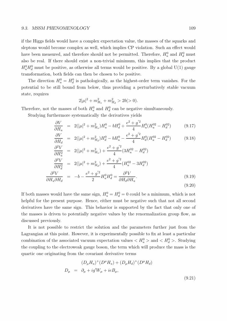
9.3. MSSM PHENOMENOLOGY 109
if the Higgs fields would have a complex expectation value, the masses of the squarks and
sleptons would become complex as well, which implies CP violation. Such an effect would
have been measured, and therefore should not be permitted. Therefore, H0u and H0
d must
also be real. If there should exist a non-trivial minimum, this implies that the product
H0uH
0d must be positive, as otherwise all terms would be positive. By a global U(1) gauge
transformation, both fields can then be chosen to be positive.
The direction H0u = H0
d is pathologically, as the highest-order term vanishes. For the
potential to be still bound from below, thus providing a perturbatively stable vacuum
state, requires
2|µ|2 +m2Hu
+m2Hd> 2b(> 0).
Therefore, not the masses of both H0u and H0
d can be negative simultaneously.
Studying furthermore systematically the derivatives yields
∂V
∂Hu
= 2(|µ|2 +m2Hu
)H0u − bH0
d +e2 + g
′2
4H0
u(H02u −H02
d ) (9.17)
∂V
∂Hd
= 2(|µ|2 +m2Hd
)H0d − bH0
u − e2 + g′2
4H0
d(H02u −H02
d ) (9.18)
∂2V
∂H2u
= 2(|µ|2 +m2Hu
) +e2 + g
′2
4(3H02
u −H02d )
∂2V
∂H2d
= 2(|µ|2 +m2Hd
) +e2 + g
′2
4(H02
u − 3H02d )
∂2V
∂Hu∂Hd
= −b − e2 + g′2
2H0
uH0d =
∂2V
∂Hd∂Hu
. (9.19)
(9.20)
If both masses would have the same sign, H0u = H0
d = 0 could be a minimum, which is not
helpful for the present purpose. Hence, either must be negative such that not all second
derivatives have the same sign. This behavior is supported by the fact that only one of
the masses is driven to potentially negative values by the renormalization group flow, as
discussed previously.
It is not possible to restrict the solution and the parameters further just from the
Lagrangian at this point. However, it is experimentally possible to fix at least a particular
combination of the associated vacuum expectation values < H0u > and < H0
d >. Studying
the coupling to the electroweak gauge boson, the term which will produce the mass is the
quartic one originating from the covariant derivative terms
(DµHu)+(DµHu) + (DµHd)
+(DµHd)
Dµ = ∂µ + ig′Wµ + ieBµ,
(9.21)

110CHAPTER 9. A PRIMER ON THE MINIMAL SUPERSYMMETRIC STANDARD MODEL
where the coupling matrices have been included into the gauge fields. This yields the
quartic contributions
(ig′Wµ + ieBµ)Hu(ig′W µ + ieBµ)Hu + (ig′Wµ + ieBµ)Hd(ig
′W µ + ieBµ)Hd.
Introducing the combination W±µ = W 1
µ ± W 2µ , Zµ = (−e′Bµ + gW µ
3 )/(e2 + g′2) (and
correspondingly the photon γµ = (e′Bµ + gW µ3 )/(e2 + g
′2)), performing the algebra, and
setting the Higgs fields to their vacuum expectation values yields3
(1
2(e2 + g
′2)ZµZµ +
1
2g2(W+
µ Wµ+ +W−
µ Wµ−))(< H0
u >2 + < H0
d >2). (9.22)
Thus, this yields the tree-level masses for the electroweak gauge bosons. The value for the
combined condensate is therefore, according to experiment, (174GeV)2.
It is furthermore possible to determine mass-bounds for the Higgs4. This is a bit more
complicated than in the standard model case, as both Higgs fields will mix. Is is therefore
useful to discuss this first for the example of two scalar fields φ1,2, which both condense
with vacuum expectation values v1,2, and which interact through some potential V (φ1, φ2).
The corresponding Lagrangian is then
L = ∂µφ1∂µφ1 + ∂µφ2∂
µφ2 − V (φ1, φ2).
Since the setting is perturbative, it is possible to expand V around the minima φi = vi to
obtain the masses and keeping only terms quadratic, yielding
L2 = ∂µφ1∂µφ1 + ∂µφ2∂
µφ2 −1
2
∂2V
∂φ21
(φ1 − v1)2
−1
2
∂2V
∂φ22
(φ2 − v2)2 − ∂2V
∂φ1∂φ2(φ1 − v1)(φ2 − v2). (9.23)
This can be simplified by setting
Φi =√
2(φi − vi)
as
L2 = −1
2ΦT∂2Φ − ΦTMΦ
3Which should be again understood to choosing a particular gauge.4It should be noted that in the following implicitly unitary gauge has been chosen. For the calculations
performed, this is not relevant, expect that it permits to expand Hu and Hd around their vacuum expec-
tation value. However, the results are therefore not necessarily gauge-invariant, and should be interpreted
with caution.

9.3. MSSM PHENOMENOLOGY 111
with
M =1
2
(
∂2V∂φ2
1
∂2V∂φ1∂φ2
∂2V∂φ1∂φ2
∂2V∂φ2
2
)
.
Since the mass-matrix M is real and symmetric, it can be diagonalized by some orthogonal
matrix
U =
(
cosα − sinα
sinα cosα
)
,
which can be used to change the basis for the fields as
(
φ+
φ−
)
= UΦ.
If the eigenvalues of M are given by m2±, the resulting Lagrangian takes the form
L2 = −1
2(φ+∂
2φ+ + φ−∂2φ− +m2
+φ2+ +m2
−φ2−),
thus making the masses for the newly defined fields explicit. It should be noted that the
matrix M has to be evaluated at φi = vi.
Returning to the Higgs fields in the minimal supersymmetric standard model, there
are eight instead of two fields, but only two out of the eight have a non-vanishing vacuum
expectation value. Examples of the relevant derivatives are given in (9.17-9.19). Using
furthermore that the vanishing of the first derivatives implies certain relations for the
values of < Hu > and < Hd >, it possible to simplify the ensuing expressions algebraically.
Finally, defining
tanβ =< Hu >
< Hd >,
the resulting expressions become relatively simple. It is furthermore useful that the mass-
matrix assumes a block-diagonal form, so that it is possible to reduce the complexity
further by studying only doublets at each time.
The first doublet to be studied are the (non-condensing) imaginary parts of H0u and
H0d . The corresponding mass-matrix takes the form
Mi0 =
(
b cot β b
b b tan β
)
,
which has eigenvalues m2+ = 0 and m2
− = 2b/ sin(2β). The massless mode, as it is un-
charged, will become effectively the longitudinal component of the Z0. The combination
√2(cosβℑ(H0
u) + sin βℑ(H0D))
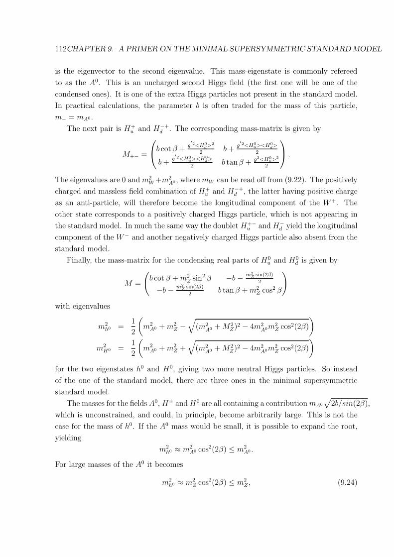
112CHAPTER 9. A PRIMER ON THE MINIMAL SUPERSYMMETRIC STANDARD MODEL
is the eigenvector to the second eigenvalue. This mass-eigenstate is commonly refereed
to as the A0. This is an uncharged second Higgs field (the first one will be one of the
condensed ones). It is one of the extra Higgs particles not present in the standard model.
In practical calculations, the parameter b is often traded for the mass of this particle,
m− = mA0 .
The next pair is H+u and H−+
d . The corresponding mass-matrix is given by
M+− =
b cot β +g′2<H0
d>2
2b+
g′2<H0
u><H0d>
2
b+g′2<H0
u><H0d>
2b tanβ + g2<H0
u>2
2
.
The eigenvalues are 0 andm2W +m2
A0 , where mW can be read off from (9.22). The positively
charged and massless field combination of H+u and H−+
d , the latter having positive charge
as an anti-particle, will therefore become the longitudinal component of the W+. The
other state corresponds to a positively charged Higgs particle, which is not appearing in
the standard model. In much the same way the doublet H+−u andH−
d yield the longitudinal
component of the W− and another negatively charged Higgs particle also absent from the
standard model.
Finally, the mass-matrix for the condensing real parts of H0u and H0
d is given by
M =
(
b cot β +m2Z sin2 β −b− m2
Zsin(2β)
2
−b− m2Z
sin(2β)
2b tanβ +m2
Z cos2 β
)
with eigenvalues
m2h0 =
1
2
(
m2A0 +m2
Z −√
(m2A0 +M2
Z)2 − 4m2A0m2
Z cos2(2β)
)
m2H0 =
1
2
(
m2A0 +m2
Z +√
(m2A0 +M2
Z)2 − 4m2A0m2
Z cos2(2β)
)
for the two eigenstates h0 and H0, giving two more neutral Higgs particles. So instead
of the one of the standard model, there are three ones in the minimal supersymmetric
standard model.
The masses for the fields A0,H± andH0 are all containing a contributionmA0
√
2b/sin(2β),
which is unconstrained, and could, in principle, become arbitrarily large. This is not the
case for the mass of h0. If the A0 mass would be small, it is possible to expand the root,
yielding
m2h0 ≈ m2
A0 cos2(2β) ≤ m2A0 .
For large masses of the A0 it becomes
m2h0 ≈ m2
Z cos2(2β) ≤ m2Z , (9.24)
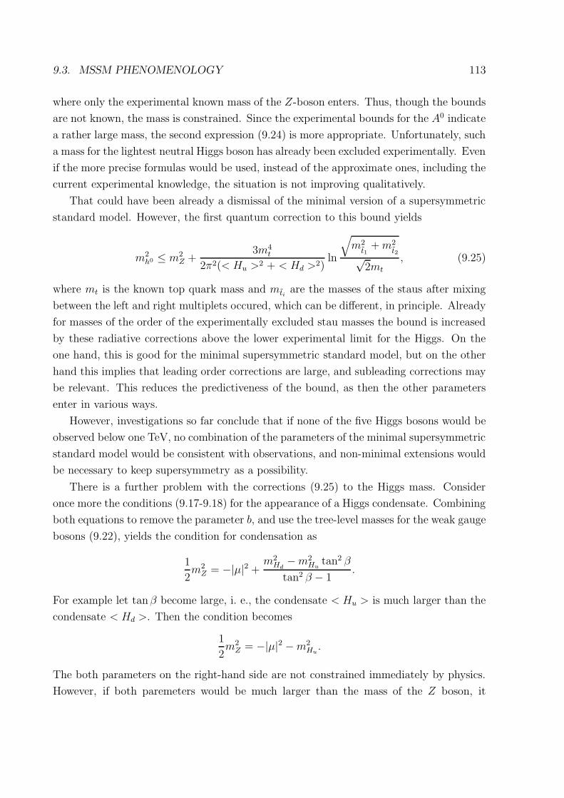
9.3. MSSM PHENOMENOLOGY 113
where only the experimental known mass of the Z-boson enters. Thus, though the bounds
are not known, the mass is constrained. Since the experimental bounds for the A0 indicate
a rather large mass, the second expression (9.24) is more appropriate. Unfortunately, such
a mass for the lightest neutral Higgs boson has already been excluded experimentally. Even
if the more precise formulas would be used, instead of the approximate ones, including the
current experimental knowledge, the situation is not improving qualitatively.
That could have been already a dismissal of the minimal version of a supersymmetric
standard model. However, the first quantum correction to this bound yields
m2h0 ≤ m2
Z +3m4
t
2π2(< Hu >2 + < Hd >2)ln
√
m2t1
+m2t2√
2mt
, (9.25)
where mt is the known top quark mass and mti are the masses of the staus after mixing
between the left and right multiplets occured, which can be different, in principle. Already
for masses of the order of the experimentally excluded stau masses the bound is increased
by these radiative corrections above the lower experimental limit for the Higgs. On the
one hand, this is good for the minimal supersymmetric standard model, but on the other
hand this implies that leading order corrections are large, and subleading corrections may
be relevant. This reduces the predictiveness of the bound, as then the other parameters
enter in various ways.
However, investigations so far conclude that if none of the five Higgs bosons would be
observed below one TeV, no combination of the parameters of the minimal supersymmetric
standard model would be consistent with observations, and non-minimal extensions would
be necessary to keep supersymmetry as a possibility.
There is a further problem with the corrections (9.25) to the Higgs mass. Consider
once more the conditions (9.17-9.18) for the appearance of a Higgs condensate. Combining
both equations to remove the parameter b, and use the tree-level masses for the weak gauge
bosons (9.22), yields the condition for condensation as
1
2m2
Z = −|µ|2 +m2
Hd−m2
Hutan2 β
tan2 β − 1.
For example let tanβ become large, i. e., the condensate < Hu > is much larger than the
condensate < Hd >. Then the condition becomes
1
2m2
Z = −|µ|2 −m2Hu.
The both parameters on the right-hand side are not constrained immediately by physics.
However, if both paremeters would be much larger than the mass of the Z boson, it

114CHAPTER 9. A PRIMER ON THE MINIMAL SUPERSYMMETRIC STANDARD MODEL
would be necessary for them to cancel almost exactly. If this would be the case, it would
immediately raise the same questions as in the original fine-tuning problem of the standard
model if the Higgs mass would be much larger than the ones of the weak bosons. This is
therefore also called the little fine-tuning or hierarchy problem.
That this is indeed somewhat of a problem becomes apparent when considering the
renormalization constant for the mass of the Higgs boson, which is given by the integral
of (9.13) approximately by
δm2Hu
≈ −3y2t
8π2(m2
t1+m2
t2) log
√2ΛU
√
m2t1
+m2t2
, (9.26)
where it was assumed that the stau masses give the dominant contributions, due to the
condition (9.25). The value of the unification scale is still of the order of 1015 GeV. If there-
fore the mass shift due to the leading quantum corrections should be small, this yields
approximately that the geometric average of the stau masses should not be larger than
about 150 GeV. Otherwise the quantum corrections alone would produce a fine-tuning
problem. This condition is, however, in violation of the bound of 500 GeV necessary
to shift the h0 Higgs boson out of the current experimental reach. Therefore, it cannot
be permitted. Shifting then the stau masses to the required value yields a mass correc-
tion large compared to the Z-mass, actually, it becomes exponentially worse due to the
logarithmic dependence. Thus a fine-tuning problem arises. Whether this constitutes a
problem, or just an aesthetic displeasure, is not only a question of personal taste. It also is
a challenge to understand whether nature prefers for what reasons theories with or without
fine tuning.
9.3.3 Mass spectrum
So far, the masses of the Higgs bosons and the electroweak bosons have been calculated.
The gluons also remain massless, in accordance with observation. The remaining mass
spectrum for the minimal supersymmetric standard model at tree-level will be discussed
in the following.
The first particles are the remaining ones from the standard model. These have to
acquire, of course, their observed masses. Due to the parity violating nature of the weak
interactions, these masses can effectively arise only due to the Yukawa interaction with the
Higgs particles. In unitary gauge, these couplings can be split into a contribution which
contains only the Higgs vacuum expectation values
yχχH = yχχ < H > +yχχ(H− < h >)

9.3. MSSM PHENOMENOLOGY 115
and behave therefore as mass terms. Thus, the masses are given by
muct = yuct < Hu >= yuct
√2mW sin β
g′
mdsb = ydsb < Hd >= ydsb
√2mW cosβ
g′
meµτ = yeµτ < Hd >= yeµτ
√2mW cosβ
g′
mνeνµντ= yνeνµντ
< Hu >= yνeνµντ
√2mW sin β
g′.
The twelve Yukawa couplings are all free parameters of the minimal supersymmetric stan-
dard model. As is visible, it strongly depends on the value of β, whether these couplings
are strong, preventing perturbative descriptions, or weak enough that at sufficiently high
energies perturbation theory is adequate.
The situation for the gluinos is actually even simpler. Since the color symmetry is
unbroken, no other fermions exist with the quantum numbers of the gluinos, and they do
not couple to the parity violating weak interactions, the only contribution comes from the
explicit supersymmetry breaking term
−1
2M1gg −
1
2M∗
1 g+g+.
The mass parameter can be complex in general, but the corresponding tree-level mass will
just be its absolute value. Therefore, the value of the mass of the gluinos is unconstrained
in the minimal supersymmetric standard model, but by virtue of relation (9.12) it is tied
to the masses of the other gauginos in case of unification.
The situation becomes more complicated for the so-called neutralinos, the superpart-
ners of W 0 and B, the wino W 0 and the bino B. These fermions are electrically uncharged,
and can both mix, similar to their standard-model versions. Furthermore, the neutral su-
perpartners of the two Higgs fields, the higgsinos H0d and H0
u are both also fermionic
and uncharged. Hence, these can mix with the binos and the winos as well. The gauge
eigenstate is therefore
G0T = (B, W 0, H0d , H
0u).
The most direct mixing is due to the interaction mediate by the weak F -boson in the
Wess-Zumino-like contribution to the superpotential, which leads to the contributions
1
2µ(H0
uH0d + H0
dH0u) +
1
2µ∗(H0+
u H0+d + H0+
d H0+u ).
Furthermore, the weak gauge symmetry and supersymmetry demand the existence of
couplings of the generic type
−√
2g′HuHuW = −√
2g′(Hu+ < Hu >)HuW (9.27)
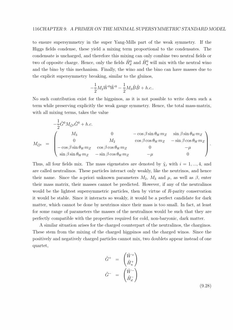
116CHAPTER 9. A PRIMER ON THE MINIMAL SUPERSYMMETRIC STANDARD MODEL
to ensure supersymmetry in the super Yang-Mills part of the weak symmetry. If the
Higgs fields condense, these yield a mixing term proportional to the condensates. The
condensate is uncharged, and therefore this mixing can only combine two neutral fields or
two of opposite charge. Hence, only the fields H0d and H0
u will mix with the neutral wino
and the bino by this mechanism. Finally, the wino and the bino can have masses due to
the explicit supersymmetry breaking, similar to the gluinos,
−1
2M2W
0W 0 − 1
2M3BB + h.c..
No such contribution exist for the higgsinos, as it is not possible to write down such a
term while preserving explicitly the weak gauge symmetry. Hence, the total mass-matrix,
with all mixing terms, takes the value
−1
2G0MG0G0 + h.c.
MG0 =
M3 0 − cosβ sin θWmZ sin β sin θWmZ
0 M2 cosβ cos θWmZ − sin β cos θWmZ
− cosβ sin θWmZ cosβ cos θWmZ 0 −µsin β sin θWmZ − sin β cos θWmZ −µ 0
.
Thus, all four fields mix. The mass eigenstates are denoted by χi with i = 1, ..., 4, and
are called neutralinos. These particles interact only weakly, like the neutrinos, and hence
their name. Since the a-priori unknown parameters M2, M3 and µ, as well as β, enter
their mass matrix, their masses cannot be predicted. However, if any of the neutralinos
would be the lightest supersymmetric particles, then by virtue of R-parity conservation
it would be stable. Since it interacts so weakly, it would be a perfect candidate for dark
matter, which cannot be done by neutrinos since their mass is too small. In fact, at least
for some range of parameters the masses of the neutralinos would be such that they are
perfectly compatible with the properties required for cold, non-baryonic, dark matter.
A similar situation arises for the charged counterpart of the neutralinos, the charginos.
These stem from the mixing of the charged higgsinos and the charged winos. Since the
positively and negatively charged particles cannot mix, two doublets appear instead of one
quartet,
G+ =
(
W+
H+u
)
G− =
(
W−
H−d
)
(9.28)

9.3. MSSM PHENOMENOLOGY 117
where the charged winos are linear combinations W 1 ± iW 2 of the off-diagonal winos.
Similar as in the case of the neutralinos, there is a contribution from the weak F -term
and the condensation of the neutral Higgs fields from the super Yang-Mills action, which
mixes both components of each doublet. Finally, there is again the explicit supersymmetry
breaking mass of the winos. All in all, the corresponding mass term is
−1
2(G+TMT
G±G− + G−TMG±G+) + h.c. (9.29)
MG± =
(
M2
√2 sin βmW√
2 cosβmW µ
)
.
The structure of the mass term is dictated by the (hypercharge) gauge symmetry. To
obtain the masses, it is necessary to diagonalize the mass-matrix, and identify the ac-
tual masses. The unitary matrices V and U are taken to transform the charged gauge
eigenstates into the chargino mass eigenstates
χ+ = V G+
χ− = UG−.
To obtain the mass eigenstates, U and V will be chosen such that U∗MG±V −1 is diagonal,
as is required to have a diagonal structure in both terms in (9.29). However, when de-
termining the associated propagators, from which the pole mass can be read off, not the
quantity U∗MG±V −1 appears, but rather the quadratic version V X+XV −1 = UXX+UT ,
as a consequence of the inversion and the structure of a fermion propagator. The equality
follows trivial from linear algebra. Performing the algebra leads to masses of the charginos
|mχ±
i|2 =
1
2
(
M22 + |µ|2 + 2m2
W ) ∓√
(M22 + |µ|2 + 2m2
W )2 − 4|µM2 −m2W sin(2β)|2
)
where the upper and lower sign refer to the two members of each charged doublet. There-
fore there is always one pair of oppositely charged charginos having the same mass, as
would be expected from CPT.
Thus remains the largest group of additional particles, the sfermion superpartners of
the fermionic standard model particles. These contain the squarks and sleptons. For-
tunately, due to the presence of the strong charge, squarks and sleptons will not mix.
However, the three families within each sector could in principle mix. Since such mixings
would have to be very small to be not in contradiction to flavor changing currents ob-
served in experiments, these will be neglected. Furthermore, compared to the scale of the
supersymmetric parameters, only the Yukawa couplings of the third family can give any
significant contribution, and will only be considered in this case. Therefore, the first two
and the third family will be treated in turns.

118CHAPTER 9. A PRIMER ON THE MINIMAL SUPERSYMMETRIC STANDARD MODEL
If a common mass at some unification scale can be expected then the masses will run
according to
m2qL
= m20 +K1 +K2 +
1
9K3
m2uR,cR
= m20 +K1 +
16
9K3
m2dR,sR
= m20 +K1 +
4
9K3
m2lL
= m20 +K2 +K3
m2eR,µR
= m20 + 4K3
m2˜νeR, ˜νµR
= m20.
The contributions Ki are the ones from the various interactions, weighted accordingly
with the corresponding weak isospin and hypercharge quantum numbers. Since to this
order the Yukawa interactions can be neglected, there are only the contributions from the
interactions which all tend to increase the mass, except for the right handed sneutrinos to
this order. The strong interaction K1 will give the largest contribution. Hence, the squark
masses will tend to be larger than the slepton masses.
On top of these contributions stemming purely from the soft breaking of the super-
symmetry, there are again additional effects from the coupling to the Higgs fields. This
coupling arises, since the equation of motion for the (weak isospin) D boson yields
D = g′(q+q+ + l+ l+ +H+u Hu +H+
d Hd),
which by virtue of the term D2 in the Lagrangian yield terms of the type
(q+q)g′2(< H0u >
2 − < H0d >
2).
Similarly, the hypercharge D boson contributes
e2−y2
(q+q)(< H0u >
2 − < H0d >
2),
where y is the corresponding weak hypercharge. In total the contribution ∆f for each
sfermion with weak isospin quantum number t3 and charge c = y/2 + t3 is
∆f = m2Z cos(2β)
(
t3 − c sin2 θW .)
As a consequence the weak isospin splittings give a measure of β as
m2dL
−m2uL
= m2eL
−m2νe
= −m2W cos(2β),
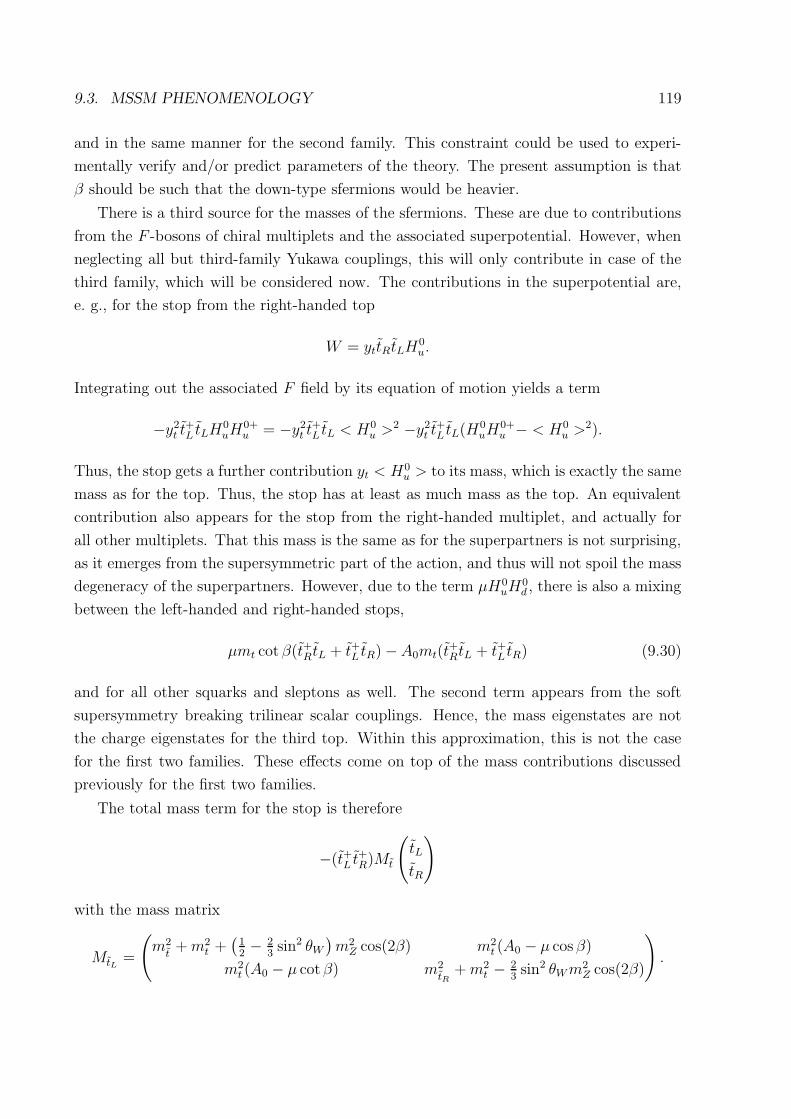
9.3. MSSM PHENOMENOLOGY 119
and in the same manner for the second family. This constraint could be used to experi-
mentally verify and/or predict parameters of the theory. The present assumption is that
β should be such that the down-type sfermions would be heavier.
There is a third source for the masses of the sfermions. These are due to contributions
from the F -bosons of chiral multiplets and the associated superpotential. However, when
neglecting all but third-family Yukawa couplings, this will only contribute in case of the
third family, which will be considered now. The contributions in the superpotential are,
e. g., for the stop from the right-handed top
W = yttRtLH0u.
Integrating out the associated F field by its equation of motion yields a term
−y2t t
+L tLH
0uH
0+u = −y2
t t+L tL < H0
u >2 −y2
t t+L tL(H0
uH0+u − < H0
u >2).
Thus, the stop gets a further contribution yt < H0u > to its mass, which is exactly the same
mass as for the top. Thus, the stop has at least as much mass as the top. An equivalent
contribution also appears for the stop from the right-handed multiplet, and actually for
all other multiplets. That this mass is the same as for the superpartners is not surprising,
as it emerges from the supersymmetric part of the action, and thus will not spoil the mass
degeneracy of the superpartners. However, due to the term µH0uH
0d , there is also a mixing
between the left-handed and right-handed stops,
µmt cot β(t+R tL + t+L tR) −A0mt(t+R tL + t+L tR) (9.30)
and for all other squarks and sleptons as well. The second term appears from the soft
supersymmetry breaking trilinear scalar couplings. Hence, the mass eigenstates are not
the charge eigenstates for the third top. Within this approximation, this is not the case
for the first two families. These effects come on top of the mass contributions discussed
previously for the first two families.
The total mass term for the stop is therefore
−(t+L t+R)Mt
(
tL
tR
)
with the mass matrix
MtL =
(
m2t+m2
t +(
12− 2
3sin2 θW
)
m2Z cos(2β) m2
t (A0 − µ cosβ)
m2t (A0 − µ cotβ) m2
tR+m2
t − 23sin2 θWm
2Z cos(2β)
)
.
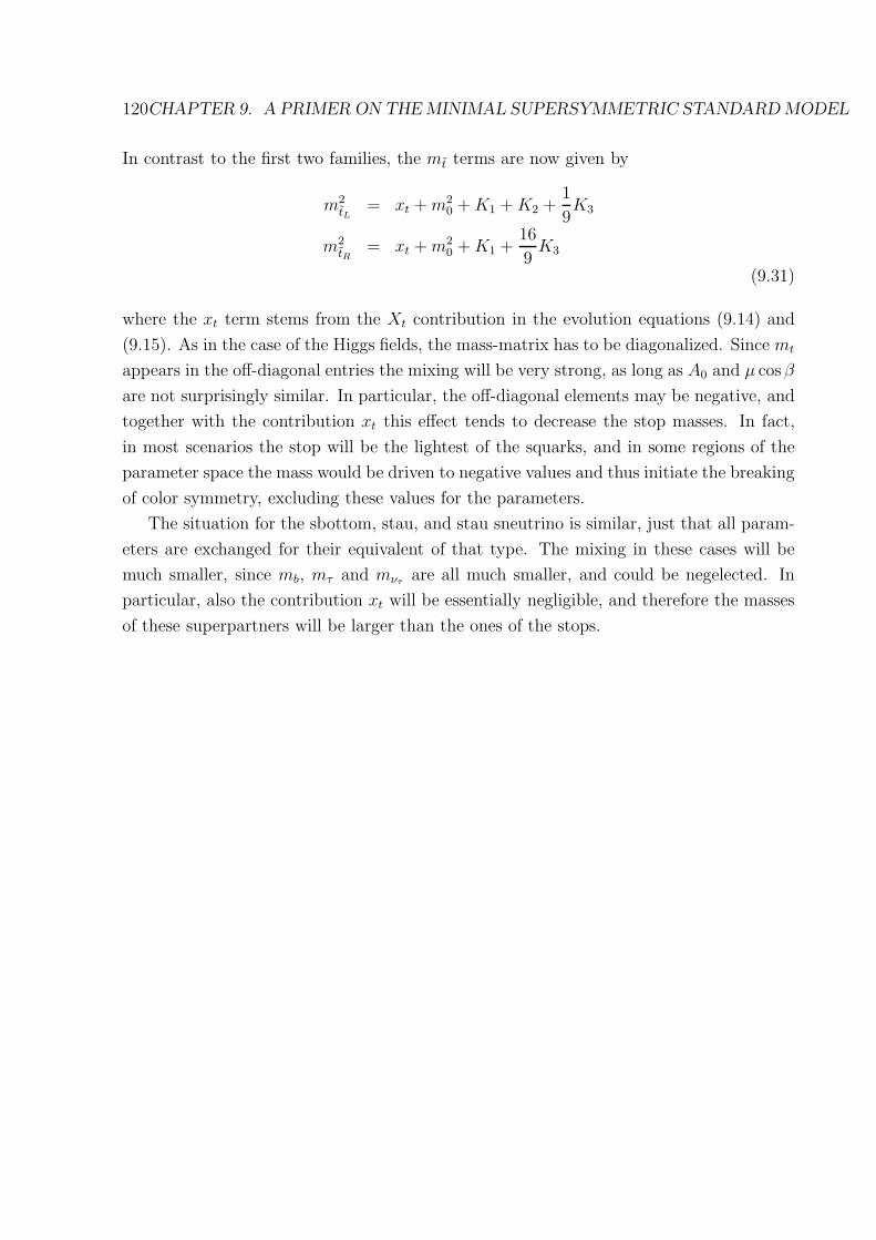
120CHAPTER 9. A PRIMER ON THE MINIMAL SUPERSYMMETRIC STANDARD MODEL
In contrast to the first two families, the mt terms are now given by
m2tL
= xt +m20 +K1 +K2 +
1
9K3
m2tR
= xt +m20 +K1 +
16
9K3
(9.31)
where the xt term stems from the Xt contribution in the evolution equations (9.14) and
(9.15). As in the case of the Higgs fields, the mass-matrix has to be diagonalized. Since mt
appears in the off-diagonal entries the mixing will be very strong, as long as A0 and µ cosβ
are not surprisingly similar. In particular, the off-diagonal elements may be negative, and
together with the contribution xt this effect tends to decrease the stop masses. In fact,
in most scenarios the stop will be the lightest of the squarks, and in some regions of the
parameter space the mass would be driven to negative values and thus initiate the breaking
of color symmetry, excluding these values for the parameters.
The situation for the sbottom, stau, and stau sneutrino is similar, just that all param-
eters are exchanged for their equivalent of that type. The mixing in these cases will be
much smaller, since mb, mτ and mντare all much smaller, and could be negelected. In
particular, also the contribution xt will be essentially negligible, and therefore the masses
of these superpartners will be larger than the ones of the stops.


![Lecture notes Introduction to Supersymmetry and Supergravityjlouis/Vorlesungen/SUSY_15/susysugra_15.pdf · 1Textbooks of supersymmetry and supergravity include [1{5]. For review lectures](https://img.dokumen.tips/doc/110x75/5f4932eb921ae62f740d2bba/lecture-notes-introduction-to-supersymmetry-and-supergravity-jlouisvorlesungensusy15susysugra15pdf.jpg)


![Introduction to supergravity - arXiv · supersymmetry, but supergravity is introduced as well. The supergravity review [3] is still, 30 years later, a very good introduction. The](https://img.dokumen.tips/doc/110x75/5ec7a9f876d4fe3f047ef2a9/introduction-to-supergravity-arxiv-supersymmetry-but-supergravity-is-introduced.jpg)


![[Wess Bagger]Supersymmetry and Supergravity](https://img.dokumen.tips/doc/110x75/55cf8eb6550346703b94d652/wess-baggersupersymmetry-and-supergravity.jpg)
