Embed Size (px)
Citation preview

Introduction to Social Network Methods: Table of Contents
http://www.faculty.ucr.edu/~hanneman/nettext/[8/21/2009 2:08:40 PM]
Robert A. Hanneman and Mark Riddle
Introduction to social network methods
Table of contents
About this book
This on-line textbook introduces many of the basics of formal approaches to the analysis of social networks. The text relies heavily on the work of Freeman, Borgatti, and Everett (the authors of the UCINET softwarepackage). The materials here, and their organization, were also very strongly influenced by the text ofWasserman and Faust, and by a graduate seminar conducted by Professor Phillip Bonacich at UCLA. Manyother users have also made very helpful comments and suggestions based on the first version. Errors andomissions, of course, are the responsibility of the authors.
You are invited to use and redistribute this text freely -- but please acknowledge the source.
Hanneman, Robert A. and Mark Riddle. 2005. Introduction to social network methods. Riverside, CA: University of California, Riverside ( published in digital form at http://faculty.ucr.edu/~hanneman/ )
Table of contents:
Preface1. Social network data2. Why formal methods?3. Using graphs to represent social relations4. Working with Netdraw to visualize graphs5. Using matrices to represent social relations6. Working with network data7. Connection8. Embedding9. Ego networks10. Centrality and power11. Cliques and sub-groups12. Positions and roles: The idea of equivalence13. Measures of similarity and structural equivalence14. Automorphic equivalence15. Regular equivalence16. Multiplex networks17. Two-mode networks18. Some statistical toolsAfter wordBibliography

Introduction to social network methods: Preface
http://www.faculty.ucr.edu/~hanneman/nettext/C0_Preface.html[8/21/2009 2:09:05 PM]
Introduction to social network methods
Preface
This page is part of an on-line text by Robert A. Hanneman (Department of Sociology, University of California, Riverside) and MarkRiddle (Department of Sociology, University of Northern Colorado). Feel free to use and distribute this textbook, with citation. Yourcomments and suggestions are very welcome. Send me e-mail.
This book began as a set of reading notes as Hanneman sought to teach himself the basics of socialnetwork analysis. It then became a set of lecture notes for students in his undergraduate course in socialnetwork analysis. Through a couple extensions and revisions, it has evolved to cover more of the basicapproaches to the analysis of social network data. Its current form, written in 2005, covers most of thealgorithms and approaches that are collected in the computer package UCINET, version 6.85. Mark Riddlehas added expertise in the statistical modeling of network data, study questions and problems, andconnections to a variety of empirical literature that uses the techniques discussed here.
Our goal in preparing this book is to provide a very basic introduction to the core ideas of social networkanalysis, and how these ideas are implemented in the methodologies that many social network analystsuse. The book is distributed free on the Internet in the hope that it may reach a diverse audience, and thatthe core ideas and methods of this field may be of interest. The book may also be suitable as course-support for undergraduate or introductory graduate training in social network analysis. While this text is not auser's guide to UCINET (which has excellent documentation in its help files), it may be of assistance to usersworking with that particular software package.
We hope that you will find things here that may stimulate your imagination. Social network analysis is acontinuously and rapidly evolving field, and is one branch of the broader study of networks and complexsystems. The concepts and techniques of social network analysis are informed by, and inform the evolutionof these broader fields. We hope that this text will serve as a starting point.
table of contents of the book
Introduction to Social Network Methods: Chapter 1: Social Network Data
http://faculty.ucr.edu/~hanneman/nettext/C1_Social_Network_Data.html[8/21/2009 2:09:28 PM]
Introduction to social network methods
1. Social network data
This page is part of an on-line text by Robert A. Hanneman (Department of Sociology, University of California, Riverside) and MarkRiddle (Department of Sociology, University of Northern Colorado). Feel free to use and distribute this textbook, with citation. Yourcomments and suggestions are very welcome. Send me e-mail.
Contents of chapter 1: Social network data
Introduction: What's different about social network data?Nodes
Populations, samples, and boundariesModality and levels of analysis
RelationsSampling tiesMultiple relations
Scales of measurementA note on statistics and social network data
Introduction: What's different about social network data?
On one hand, there really isn't anything about social network data that is all that unusual. Social networkanalysts do use a specialized language for describing the structure and contents of the sets of observationsthat they use. But, network data can also be described and understood using the ideas and concepts ofmore familiar methods, like cross-sectional survey research.
On the other hand, the data sets that social network analysts develop usually end up looking quite differentfrom the conventional rectangular data array so familiar to survey researchers and statistical analysts. Thedifferences are quite important because they lead us to look at our data in a different way -- and even leadus to think differently about how to apply statistics.
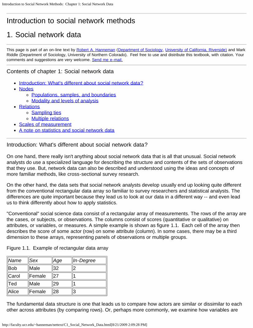
"Conventional" social science data consist of a rectangular array of measurements. The rows of the array arethe cases, or subjects, or observations. The columns consist of scores (quantitative or qualitative) onattributes, or variables, or measures. A simple example is shown as figure 1.1. Each cell of the array thendescribes the score of some actor (row) on some attribute (column). In some cases, there may be a thirddimension to these arrays, representing panels of observations or multiple groups.
Figure 1.1. Example of rectangular data array
Name Sex Age In-DegreeBob Male 32 2Carol Female 27 1Ted Male 29 1Alice Female 28 3
The fundamental data structure is one that leads us to compare how actors are similar or dissimilar to eachother across attributes (by comparing rows). Or, perhaps more commonly, we examine how variables are
Introduction to Social Network Methods: Chapter 1: Social Network Data
http://faculty.ucr.edu/~hanneman/nettext/C1_Social_Network_Data.html[8/21/2009 2:09:28 PM]
similar or dissimilar to each other in their distributions across actors (by comparing or correlating columns).
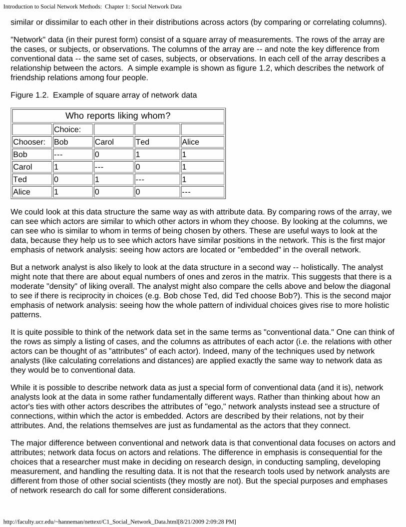
"Network" data (in their purest form) consist of a square array of measurements. The rows of the array arethe cases, or subjects, or observations. The columns of the array are -- and note the key difference fromconventional data -- the same set of cases, subjects, or observations. In each cell of the array describes arelationship between the actors. A simple example is shown as figure 1.2, which describes the network offriendship relations among four people.
Figure 1.2. Example of square array of network data
Who reports liking whom? Choice: Chooser: Bob Carol Ted AliceBob --- 0 1 1Carol 1 --- 0 1Ted 0 1 --- 1Alice 1 0 0 ---
We could look at this data structure the same way as with attribute data. By comparing rows of the array, wecan see which actors are similar to which other actors in whom they choose. By looking at the columns, wecan see who is similar to whom in terms of being chosen by others. These are useful ways to look at thedata, because they help us to see which actors have similar positions in the network. This is the first majoremphasis of network analysis: seeing how actors are located or "embedded" in the overall network.
But a network analyst is also likely to look at the data structure in a second way -- holistically. The analystmight note that there are about equal numbers of ones and zeros in the matrix. This suggests that there is amoderate "density" of liking overall. The analyst might also compare the cells above and below the diagonalto see if there is reciprocity in choices (e.g. Bob chose Ted, did Ted choose Bob?). This is the second majoremphasis of network analysis: seeing how the whole pattern of individual choices gives rise to more holisticpatterns.
It is quite possible to think of the network data set in the same terms as "conventional data." One can think ofthe rows as simply a listing of cases, and the columns as attributes of each actor (i.e. the relations with otheractors can be thought of as "attributes" of each actor). Indeed, many of the techniques used by networkanalysts (like calculating correlations and distances) are applied exactly the same way to network data asthey would be to conventional data.
While it is possible to describe network data as just a special form of conventional data (and it is), networkanalysts look at the data in some rather fundamentally different ways. Rather than thinking about how anactor's ties with other actors describes the attributes of "ego," network analysts instead see a structure ofconnections, within which the actor is embedded. Actors are described by their relations, not by theirattributes. And, the relations themselves are just as fundamental as the actors that they connect.
The major difference between conventional and network data is that conventional data focuses on actors andattributes; network data focus on actors and relations. The difference in emphasis is consequential for thechoices that a researcher must make in deciding on research design, in conducting sampling, developingmeasurement, and handling the resulting data. It is not that the research tools used by network analysts aredifferent from those of other social scientists (they mostly are not). But the special purposes and emphasesof network research do call for some different considerations.

Introduction to Social Network Methods: Chapter 1: Social Network Data
http://faculty.ucr.edu/~hanneman/nettext/C1_Social_Network_Data.html[8/21/2009 2:09:28 PM]
In this chapter, we will take a look at some of the issues that arise in design, sampling, and measurement forsocial network analysis. Our discussion will focus on the two parts of network data: nodes (or actors) andedges (or relations). We will try to show some of the ways in which network data are similar to, and differentfrom more familiar actor by attribute data. We will introduce some new terminology that makes it easier todescribe the special features of network data. Lastly, we will briefly discuss how the differences betweennetwork and actor-attribute data are consequential for the application of statistical tools.
table of contents
Nodes
Network data are defined by actors and by relations (or "nodes" and "edges"). The nodes or actors part ofnetwork data would seem to be pretty straight-forward. Other empirical approaches in the social sciencesalso think in terms of cases or subjects or sample elements and the like. There is one difference with mostnetwork data, however, that makes a big difference in how such data are usually collected -- and the kinds ofsamples and populations that are studied.
Network analysis focuses on the relations among actors, and not individual actors and their attributes. Thismeans that the actors are usually not sampled independently, as in many other kinds of studies (mosttypically, surveys). Suppose we are studying friendship ties, for example. John has been selected to be inour sample. When we ask him, John identifies seven friends. We need to track down each of those sevenfriends and ask them about their friendship ties, as well. The seven friends are in our sample because Johnis (and vice-versa), so the "sample elements" are no longer "independent."
The nodes or actors included in non-network studies tend to be the result of independent probabilitysampling. Network studies are much more likely to include all of the actors who occur within some (usuallynaturally occurring) boundary. Often network studies don't use "samples" at all, at least in the conventionalsense. Rather, they tend to include all of the actors in some population or populations. Of course, thepopulations included in a network study may be a sample of some larger set of populations. For example,when we study patterns of interaction among students in a classrooms, we include all of the children in aclassroom (that is, we study the whole population of the classroom). The classroom itself, though, might havebeen selected by probability methods from a population of classrooms (say all of those in a school).
The use of whole populations as a way of selecting observations in (many) network studies makes itimportant for the analyst to be clear about the boundaries of each population to be studied, and howindividual units of observation are to be selected within that population. Network data sets also frequentlyinvolve several levels of analysis, with actors embedded at the lowest level (i.e. network designs can bedescribed using the language of "nested" designs).
table of contents
Populations, samples, and boundaries
Social network analysts rarely draw samples in their work. Most commonly, network analysts will identifysome population and conduct a census (i.e. include all elements of the population as units of observation). Anetwork analyst might examine all of the nouns and objects occurring in a text, all of the persons at abirthday party, all members of a kinship group, of an organization, neighborhood, or social class (e.g.landowners in a region, or royalty).
Survey research methods usually use a quite different approach to deciding which nodes to study. A list ismade of all nodes (sometimes stratified or clustered), and individual elements are selected by probabilitymethods. The logic of the method treats each individual as a separate "replication" that is, in a sense,
Introduction to Social Network Methods: Chapter 1: Social Network Data
http://faculty.ucr.edu/~hanneman/nettext/C1_Social_Network_Data.html[8/21/2009 2:09:28 PM]
interchangeable with any other.
Because network methods focus on relations among actors, actors cannot be sampled independently to beincluded as observations. If one actor happens to be selected, then we must also include all other actors towhom our ego has (or could have) ties. As a result, network approaches tend to study whole populations bymeans of census, rather than by sample (we will discuss a number of exceptions to this shortly, under thetopic of sampling ties).
The populations that network analysts study are remarkably diverse. At one extreme, they might consist ofsymbols in texts or sounds in verbalizations; at the other extreme, nations in the world system of states mightconstitute the population of nodes. Perhaps most common, of course, are populations of individual persons.In each case, however, the elements of the population to be studied are defined by falling within someboundary.
The boundaries of the populations studied by network analysts are of two main types. Probably mostcommonly, the boundaries are those imposed or created by the actors themselves. All the members of aclassroom, organization, club, neighborhood, or community can constitute a population. These are naturallyoccurring clusters, or networks. So, in a sense, social network studies often draw the boundaries around apopulation that is known, a priori, to be a network. Alternatively, a network analyst might take a more"demographic" or "ecological" approach to defining population boundaries. We might draw observations bycontacting all of the people who are found in a bounded spatial area, or who meet some criterion (havinggross family incomes over $1,000,000 per year). Here, we might have reason to suspect that networks exist,but the entity being studied is an abstract aggregation imposed by the investigator -- rather than a pattern ofinstitutionalized social action that has been identified and labeled by its participants.
Network analysts can expand the boundaries of their studies by replicating populations. Rather than studyingone neighborhood, we can study several. This type of design (which could use sampling methods to selectpopulations) allows for replication and for testing of hypotheses by comparing populations. A second, andequally important way that network studies expand their scope is by the inclusion of multiple levels ofanalysis, or modalities.
table of contents
Modality and levels of analysis
The network analyst tends to see individual people nested within networks of face-to-face relations withother persons. Often these networks of interpersonal relations become "social facts" and take on a life oftheir own. A family, for example, is a network of close relations among a set of people. But this particularnetwork has been institutionalized and given a name and reality beyond that of its component nodes.Individuals in their work relations may be seen as nested within organizations; in their leisure relations theymay be nested in voluntary associations. Neighborhoods, communities, and even societies are, to varyingdegrees, social entities in and of themselves. And, as social entities, they may form ties with the individualsnested within them, and with other social entities.
Often network data sets describe the nodes and relations among nodes for a single bounded population. If Istudy the friendship patterns among students in a classroom, I am doing a study of this type. But a classroomexists within a school - which might be thought of as a network relating classes and other actors (principals,administrators, librarians, etc.). And most schools exist within school districts, which can be thought of asnetworks of schools and other actors (school boards, research wings, purchasing and personneldepartments, etc.). There may even be patterns of ties among school districts (say by the exchange ofstudents, teachers, curricular materials, etc.).

Introduction to Social Network Methods: Chapter 1: Social Network Data
http://faculty.ucr.edu/~hanneman/nettext/C1_Social_Network_Data.html[8/21/2009 2:09:28 PM]
Most social network analysts think of individual persons as being embedded in networks that are embeddedin networks that are embedded in networks. Network analysts describe such structures as "multi-modal." Inour school example, individual students and teachers form one mode, classrooms a second, schools a third,and so on. A data set that contains information about two types of social entities (say persons andorganizations) is a two mode network.
Of course, this kind of view of the nature of social structures is not unique to social network analystst.Statistical analysts deal with the same issues as "hierarchical" or "nested" designs. Theorists speak of themacro-meso-micro levels of analysis, or develop schema for identifying levels of analysis (individual, group,organization, community, institution, society, global order being perhaps the most commonly used system insociology). One advantage of network thinking and method is that it naturally predisposes the analyst tofocus on multiple levels of analysis simultaneously. That is, the network analyst is always interested in howthe individual is embedded within a structure and how the structure emerges from the micro-relationsbetween individual parts. The ability of network methods to map such multi-modal relations is, at leastpotentially, a step forward in rigor.
Having claimed that social network methods are particularly well suited for dealing with multiple levels ofanalysis and multi-modal data structures, it must immediately be admitted that social network analysis rarelyactually takes much advantage. Most network analyses does move us beyond simple micro or macroreductionism -- and this is good. Few, if any, data sets and analyses, however, have attempted to work atmore than two modes simultaneously. And, even when working with two modes, the most common strategyis to examine them more or less separately (one exception to this is the conjoint analysis of two modenetworks). In chapter 17, we'll take a look at some methods for multi-mode networks.
table of contents
Relations
The other half of the design of network data has to do with what ties or relations are to be measured for theselected nodes. There are two main issues to be discussed here. In many network studies, all of the ties of agiven type among all of the selected nodes are studied -- that is, a census is conducted. But, sometimesdifferent approaches are used (because they are less expensive, or because of a need to generalize) thatsample ties. There is also a second kind of sampling of ties that always occurs in network data. Any set ofactors might be connected by many different kinds of ties and relations (e.g. students in a classroom mightlike or dislike each other, they might play together or not, they might share food or not, etc.). When wecollect network data, we are usually selecting, or sampling, from among a set of kinds of relations that wemight have measured.
table of contents
Sampling ties
Given a set of actors or nodes, there are several strategies for deciding how to go about collectingmeasurements on the relations among them. At one end of the spectrum of approaches are "full network"methods. This approach yields the maximum of information, but can also be costly and difficult to execute,and may be difficult to generalize. At the other end of the spectrum are methods that look quite like thoseused in conventional survey research. These approaches yield considerably less information about networkstructure, but are often less costly, and often allow easier generalization from the observations in the sampleto some larger population. There is no one "right" method for all research questions and problems.
Full network methods require that we collect information about each actor's ties with all other actors. In

Introduction to Social Network Methods: Chapter 1: Social Network Data
http://faculty.ucr.edu/~hanneman/nettext/C1_Social_Network_Data.html[8/21/2009 2:09:28 PM]
essence, this approach is taking a census of ties in a population of actors -- rather than a sample. Forexample we could collect data on shipments of copper between all pairs of nation states in the world systemfrom International Monetary Fund records; we could examine the boards of directors of all publiccorporations for overlapping directors; we could count the number of vehicles moving between all pairs ofcities; we could look at the flows of e-mail between all pairs of employees in a company; we could ask eachchild in a play group to identify their friends.
Because we collect information about ties between all pairs or dyads, full network data give a completepicture of relations in the population. Most of the special approaches and methods of network analysis thatwe will discuss in the remainder of this text were developed to be used with full network data. Full networkdata is necessary to properly define and measure many of the structural concepts of network analysis (e.g.between-ness).
Full network data allows for very powerful descriptions and analyses of social structures. Unfortunately, fullnetwork data can also be very expensive and difficult to collect. Obtaining data from every member of apopulation, and having every member rank or rate every other member can be very challenging tasks in anybut the smallest groups. The task is made more manageable by asking respondents to identify a limitednumber of specific individuals with whom they have ties. These lists can then be compiled and cross-connected. But, for large groups (say all the people in a city), the task is practically impossible.
In many cases, the problems are not quite as severe as one might imagine. Most persons, groups, andorganizations tend to have limited numbers of ties -- or at least limited numbers of strong ties. This isprobably because social actors have limited resources, energy, time, and cognitive capacity -- and cannotmaintain large numbers of strong ties. It is also true that social structures can develop a considerable degreeof order and solidarity with relatively few connections.
Snowball methods begin with a focal actor or set of actors. Each of these actors is asked to name some orall of their ties to other actors. Then, all the actors named (who were not part of the original list) are trackeddown and asked for some or all of their ties. The process continues until no new actors are identified, or untilwe decide to stop (usually for reasons of time and resources, or because the new actors being named arevery marginal to the group we are trying to study).
The snowball method can be particularly helpful for tracking down "special" populations (often numericallysmall sub-sets of people mixed in with large numbers of others). Business contact networks, communityelites, deviant sub-cultures, avid stamp collectors, kinship networks, and many other structures can be prettyeffectively located and described by snowball methods. It is sometimes not as difficult to achieve closure insnowball "samples" as one might think. The limitations on the numbers of strong ties that most actors have,and the tendency for ties to be reciprocated often make it fairly easy to find the boundaries.
There are two major potential limitations and weaknesses of snowball methods. First, actors who are notconnected (i.e. "isolates") are not located by this method. The presence and numbers of isolates can be avery important feature of populations for some analytic purposes. The snowball method may tend tooverstate the "connectedness" and "solidarity" of populations of actors. Second, there is no guaranteed wayof finding all of the connected individuals in the population. Where does one start the snowball rolling? If westart in the wrong place or places, we may miss whole sub-sets of actors who are connected -- but notattached to our starting points.
Snowball approaches can be strengthened by giving some thought to how to select the initial nodes. In manystudies, there may be a natural starting point. In community power studies, for example, it is common tobegin snowball searches with the chief executives of large economic, cultural, and political organizations.While such an approach will miss most of the community (those who are "isolated" from the elite network),the approach is very likely to capture the elite network quite effectively.

Introduction to Social Network Methods: Chapter 1: Social Network Data
http://faculty.ucr.edu/~hanneman/nettext/C1_Social_Network_Data.html[8/21/2009 2:09:28 PM]
Ego-centric networks (with alter connections)
In many cases it will not be possible (or necessary) to track down the full networks beginning with focalnodes (as in the snowball method). An alternative approach is to begin with a selection of focal nodes (egos),and identify the nodes to which they are connected. Then, we determine which of the nodes identified in thefirst stage are connected to one another. This can be done by contacting each of the nodes; sometimes wecan ask ego to report which of the nodes that it is tied to are tied to one another.
This kind of approach can be quite effective for collecting a form of relational data from very largepopulations, and can be combined with attribute-based approaches. For example, we might take a simplerandom sample of male college students and ask them to report who are their close friends, and which ofthese friends know one another. This kind of approach can give us a good and reliable picture of the kinds ofnetworks (or at least the local neighborhoods) in which individuals are embedded. We can find out suchthings as how many connections nodes have, and the extent to which these nodes are close-knit groups.Such data can be very useful in helping to understand the opportunities and constraints that ego has as aresult of the way they are embedded in their networks.
The ego-centered approach with alter connections can also give us some information about the network as awhole, though not as much as snowball or census approaches. Such data are, in fact, micro-network datasets -- samplings of local areas of larger networks. Many network properties -- distance, centrality, andvarious kinds of positional equivalence cannot be assessed with ego-centric data. Some properties, such asoverall network density can be reasonably estimated with ego-centric data. Some properties -- such as theprevalence of reciprocal ties, cliques, and the like can be estimated rather directly.
Ego-centric networks (ego only)
Ego-centric methods really focus on the individual, rather than on the network as a whole. By collectinginformation on the connections among the actors connected to each focal ego, we can still get a pretty goodpicture of the "local" networks or "neighborhoods" of individuals. Such information is useful for understandinghow networks affect individuals, and they also give a (incomplete) picture of the general texture of thenetwork as a whole.
Suppose, however, that we only obtained information on ego's connections to alters -- but not information onthe connections among those alters. Data like these are not really "network" data at all. That is, they cannotbe represented as a square actor-by-actor array of ties. But doesn't mean that ego-centric data withoutconnections among the alters are of no value for analysts seeking to take a structural or network approach tounderstanding actors. We can know, for example, that some actors have many close friends and kin, andothers have few. Knowing this, we are able to understand something about the differences in the actorsplaces in social structure, and make some predictions about how these locations constrain their behavior.What we cannot know from ego-centric data with any certainty is the nature of the macro-structure or thewhole network.
In ego-centric networks, the alters identified as connected to each ego are probably a set that isunconnected with those for each other ego. While we cannot assess the overall density or connectedness ofthe population, we can sometimes be a bit more general. If we have some good theoretical reason to thinkabout alters in terms of their social roles, rather than as individual occupants of social roles, ego-centerednetworks can tell us a good bit about local social structures. For example, if we identify each of the altersconnected to an ego by a friendship relation as "kin," "co-worker," "member of the same church," etc., wecan build up a picture of the networks of social positions (rather than the networks of individuals) in whichegos are embedded. Such an approach, of course, assumes that such categories as "kin" are real andmeaningful determinants of patterns of interaction.

Introduction to Social Network Methods: Chapter 1: Social Network Data
http://faculty.ucr.edu/~hanneman/nettext/C1_Social_Network_Data.html[8/21/2009 2:09:28 PM]
table of contents
Multiple relations
In a conventional actor-by-trait data set, each actor is described by many variables (and each variable isrealized in many actors). In the most common social network data set of actor-by-actor ties, only one kind ofrelation is described. Just as we often are interested in multiple attributes of actors, we are often interested inmultiple kinds of ties that connect actors in a network.
In thinking about the network ties among faculty in an academic department, for example, we might beinterested in which faculty have students in common, serve on the same committees, interact as friendsoutside of the workplace, have one or more areas of expertise in common, and co-author papers. Thepositions that actors hold in the web of group affiliations are multi-faceted. Positions in one set of relationsmay re-enforce or contradict positions in another (I might share friendship ties with one set of people withwhom I do not work on committees, for example). Actors may be tied together closely in one relationalnetwork, but be quite distant from one another in a different relational network. The locations of actors inmulti-relational networks and the structure of networks composed of multiple relations are some of the mostinteresting (and still relatively unexplored) areas of social network analysis.
When we collect social network data about certain kinds of relations among actors we are, in a sense,sampling from a population of possible relations. Usually our research question and theory indicate which ofthe kinds of relations among actors are the most relevant to our study, and we do not sample -- but ratherselect -- relations. In a study concerned with economic dependency and growth, for example, I could collectdata on the exchange of performances by musicians between nations -- but it is not really likely to be all thatrelevant.
If we do not know what relations to examine, how might we decide? There are a number of conceptualapproaches that might be of assistance. Systems theory, for example, suggests two domains: material andinformational. Material things are "conserved" in the sense that they can only be located at one node of thenetwork at a time. Movements of people between organizations, money between people, automobilesbetween cities, and the like are all examples of material things which move between nodes -- and henceestablish a network of material relations. Informational things, to the systems theorist, are "non-conserved" inthe sense that they can be in more than one place at the same time. If I know something and share it withyou, we both now know it. In a sense, the commonality that is shared by the exchange of information mayalso be said to establish a tie between two nodes. One needs to be cautious here, however, not to confusethe simple possession of a common attribute (e.g. gender) with the presence of a tie (e.g. the exchange ofviews between two persons on issues of gender).
Methodologies for working with multi-relational data are not as well developed as those for working withsingle relations. Many interesting areas of work such as network correlation, multi-dimensional scaling andclustering, and role algebras have been developed to work with multi-relational data. For the most part, thesetopics are beyond the scope of the current text, and are best approached after the basics of working withsingle relational networks are mastered. We will look at some methods for multi-relational (a.k.a. "multiplex"network data in chapter 16).
table of contents
Scales of measurement
Like other kinds of data, the information we collect about ties between actors can be measured (i.e. we canassign scores to our observations) at different "levels of measurement." The different levels of measurement

Introduction to Social Network Methods: Chapter 1: Social Network Data
http://faculty.ucr.edu/~hanneman/nettext/C1_Social_Network_Data.html[8/21/2009 2:09:28 PM]
are important because they limit the kinds of questions that can be examined by the researcher. Scales ofmeasurement are also important because different kinds of scales have different mathematical properties,and call for different algorithms in describing patterns and testing inferences about them.
It is conventional to distinguish nominal, ordinal, and interval levels of measurement (the ratio level can, forall practical purposes, be grouped with interval). It is useful, however, to further divide nominal measurementinto binary and multi-category variations; it is also useful to distinguish between full-rank ordinal measuresand grouped ordinal measures. We will briefly describe all of these variations, and provide examples of howthey are commonly applied in social network studies.
Binary measures of relations: By far the most common approach to scaling (assigning numbers to)relations is to simply distinguish between relations being absent (coded zero), and ties being present (codedone). If we ask respondents in a survey to tell us "which other people on this list do you like?" we are doingbinary measurement. Each person from the list that is selected is coded one. Those who are not selected arecoded zero.
Much of the development of graph theory in mathematics, and many of the algorithms for measuringproperties of actors and networks have been developed for binary data. Binary data is so widely used innetwork analysis that it is not unusual to see data that are measured at a "higher" level transformed intobinary scores before analysis proceeds. To do this, one simply selects some "cut point" and re-scores casesas below the cut-point (zero) or above it (one). Dichotomizing data in this way is throwing away information.The analyst needs to consider what is relevant (i.e. what is the theory about? is it about the presence andpattern of ties, or about the strengths of ties?), and what algorithms are to be applied in deciding whether it isreasonable to recode the data. Very often, the additional power and simplicity of analysis of binary data is"worth" the cost in information lost.
Multiple-category nominal measures of relations: In collecting data we might ask our respondents to lookat a list of other people and tell us: "for each person on this list, select the category that describes yourrelationship with them the best: friend, lover, business relationship, kin, or no relationship." We might scoreeach person on the list as having a relationship of type "1" type "2" etc. This kind of a scale is nominal orqualitative -- each person's relationship to the subject is coded by its type, rather than its strength. Unlike thebinary nominal (true-false) data, the multiple category nominal measure is multiple choice.
The most common approach to analyzing multiple-category nominal measures is to use it to create a seriesof binary measures. That is, we might take the data arising from the question described above and createseparate sets of scores for friendship ties, for lover ties, for kin ties, etc. This is very similar to "dummycoding" as a way of handling multiple choice types of measures in statistical analysis. In examining theresulting data, however, one must remember that each node was allowed to have a tie in at most one of theresulting networks. That is, a person can be a friendship tie or a lover tie -- but not both -- as a result of theway we asked the question. In examining the resulting networks, densities may be artificially low, and therewill be an inherent negative correlation among the matrices.
This sort of multiple choice data can also be "binarized." That is, we can ignore what kind of tie is reported,and simply code whether a tie exists for a dyad, or not. This may be fine for some analyses -- but it doeswaste information. One might also wish to regard the types of ties as reflecting some underlying continuousdimension (for example, emotional intensity). The types of ties can then be scaled into a single groupedordinal measure of tie strength. The scaling, of course, reflects the predispositions of the analyst -- not thereports of the respondents.
Grouped ordinal measures of relations: One of the earliest traditions in the study of social networks askedrespondents to rate each of a set of others as "liked" "disliked" or "neutral." The result is a grouped ordinalscale (i.e., there can be more than one "liked" person, and the categories reflect an underlying rank order of

Introduction to Social Network Methods: Chapter 1: Social Network Data
http://faculty.ucr.edu/~hanneman/nettext/C1_Social_Network_Data.html[8/21/2009 2:09:28 PM]
intensity). Usually, this kind of three point scale was coded -1, 0, and +1 to reflect negative liking,indifference, and positive liking. When scored this way, the pluses and minuses make it fairly easy to writealgorithms that will count and describe various network properties (e.g. the structural balance of the graph).
Grouped ordinal measures can be used to reflect a number of different quantitative aspects of relations.Network analysts are often concerned with describing the "strength" of ties. But, "strength" may mean (someor all of) a variety of things. One dimension is the frequency of interaction -- do actors have contact daily,weekly, monthly, etc. Another dimension is "intensity," which usually reflects the degree of emotional arousalassociated with the relationship (e.g. kin ties may be infrequent, but carry a high "emotional charge" becauseof the highly ritualized and institutionalized expectations). Ties may be said to be stronger if they involvemany different contexts or types of ties. Summing nominal data about the presence or absence of multipletypes of ties gives rise to an ordinal (actually, interval) scale of one dimension of tie strength. Ties are alsosaid to be stronger to the extent that they are reciprocated. Normally we would assess reciprocity by askingeach actor in a dyad to report their feelings about the other. However, one might also ask each actor for theirperceptions of the degree of reciprocity in a relation: Would you say that neither of you like each other verymuch, that you like X more than X likes you, that X likes you more than you like X, or that you both like eachother about equally?
Ordinal scales of measurement contain more information than nominal. That is, the scores reflect finergradations of tie strength than the simple binary "presence or absence." This would seem to be a good thing,yet it is frequently difficult to take advantage of ordinal data. The most commonly used algorithms for theanalysis of social networks have been designed for binary data. Many have been adapted to continuous data-- but for interval, rather than ordinal scales of measurement. Ordinal data, consequently, are often binarizedby choosing some cut-point and re-scoring. Alternatively, ordinal data are sometimes treated as though theyreally were interval. The former strategy has some risks, in that choices of cut-points can be consequential;the latter strategy has some risks, in that the intervals separating points on an ordinal scale may be veryheterogeneous.
Full-rank ordinal measures of relations: Sometimes it is possible to score the strength of all of therelations of an actor in a rank order from strongest to weakest. For example, I could ask each respondent towrite a "1" next to the name of the person in the class that you like the most, a "2" next to the name of theperson you like next most, etc. The kind of scale that would result from this would be a "full rank order scale."Such scales reflect differences in degree of intensity, but not necessarily equal differences -- that is, thedifference between my first and second choices is not necessarily the same as the difference between mysecond and third choices. Each relation, however, has a unique score (1st, 2nd, 3rd, etc.).
Full rank ordinal measures are somewhat uncommon in the social networks research literature, as they arein most other traditions. Consequently, there are relatively few methods, definitions, and algorithms that takespecific and full advantage of the information in such scales. Most commonly, full rank ordinal measures aretreated as if they were interval. There is probably somewhat less risk in treating fully rank ordered measures(compared to grouped ordinal measures) as though they were interval, though the assumption is still a riskyone. Of course, it is also possible to group the rank order scores into groups (i.e. produce a grouped ordinalscale) or dichotomize the data (e.g. the top three choices might be treated as ties, the remainder as non-ties). In combining information on multiple types of ties, it is frequently necessary to simplify full rank orderscales. But, if we have a number of full rank order scales that we may wish to combine to form a scale (i.e.rankings of people's likings of other in the group, frequency of interaction, etc.), the sum of such scales intoan index is plausibly treated as a truly interval measure.
Interval measures of relations: The most "advanced" level of measurement allows us to discriminateamong the relations reported in ways that allow us to validly state that, for example, "this tie is twice as strongas that tie." Ties are rated on scales in which the difference between a "1" and a "2" reflects the same

Introduction to Social Network Methods: Chapter 1: Social Network Data
http://faculty.ucr.edu/~hanneman/nettext/C1_Social_Network_Data.html[8/21/2009 2:09:28 PM]
amount of real difference as that between "23" and "24."
True interval level measures of the strength of many kinds of relationships are fairly easy to construct, with alittle imagination and persistence. Asking respondents to report the details of the frequency or intensity ofties by survey or interview methods, however, can be rather unreliable -- particularly if the relationships beingtracked are not highly salient and infrequent. Rather than asking whether two people communicate, onecould count the number of email, phone, and inter-office mail deliveries between them. Rather than askingwhether two nations trade with one another, look at statistics on balances of payments. In many cases, it ispossible to construct interval level measures of relationship strength by using artifacts (e.g. statisticscollected for other purposes) or observation.
Continuous measures of the strengths of relationships allow the application of a wider range of mathematicaland statistical tools to the exploration and analysis of the data. Many of the algorithms that have beendeveloped by social network analysts, originally for binary data, have been extended to take advantage ofthe information available in full interval measures. Whenever possible, connections should be measured atthe interval level -- as we can always move to a less refined approach later; if data are collected at thenominal level, it is much more difficult to move to a more refined level.
Even though it is a good idea to measure relationship intensity at the most refined level possible, mostnetwork analysis does not operate at this level. The most powerful insights of network analysis, and many ofthe mathematical and graphical tools used by network analysts were developed for simple graphs (i.e. binary,undirected). Many characterizations of the embeddedness of actors in their networks, and of the networksthemselves are most commonly thought of in discrete terms in the research literature. As a result, it is oftendesirable to reduce even interval data to the binary level by choosing a cutting -point, and coding tie strengthabove that point as "1" and below that point as "0." Unfortunately, there is no single "correct" way to choose acut-point. Theory and the purposes of the analysis provide the best guidance. Sometimes examining thedata can help (maybe the distribution of tie strengths really is discretely bi-modal, and displays a clear cutpoint; maybe the distribution is highly skewed and the main feature is a distinction between no tie and anytie). When a cut-point is chosen, it is wise to also consider alternative values that are somewhat higher andlower, and repeat the analyses with different cut-points to see if the substance of the results is affected. Thiscan be very tedious, but it is very necessary. Otherwise, one may be fooled into thinking that a real patternhas been found, when we have only observed the consequences of where we decided to put our cut-point.
table of contents
A note on statistics and social network data
Social network analysis is more a branch of "mathematical" sociology than of "statistical or quantitativeanalysis," though social network analysts most certainly practice both approaches. The distinction betweenthe two approaches is not clear-cut. Mathematical approaches to network analysis tend to treat the data as"deterministic." That is, they tend to regard the measured relationships and relationship strengths asaccurately reflecting the "real" or "final" or "equilibrium" status of the network. Mathematical types also tendto assume that the observations are not a "sample" of some larger population of possible observations;rather, the observations are usually regarded as the population of interest. Statistical analysts tend to regardthe particular scores on relationship strengths as stochastic or probabilistic realizations of an underlying truetendency or probability distribution of relationship strengths. Statistical analysts also tend to think of aparticular set of network data as a "sample" of a larger class or population of such networks or networkelements -- and have a concern for the results of the current study would be reproduced in the "next" study ofsimilar samples.
In the chapters that follow in this text, we will mostly be concerned with the "mathematical" rather than the"statistical" side of network analysis (again, it is important to remember that I am over-drawing the

Introduction to Social Network Methods: Chapter 1: Social Network Data
http://faculty.ucr.edu/~hanneman/nettext/C1_Social_Network_Data.html[8/21/2009 2:09:28 PM]
differences in this discussion). Before passing on to this, we should note a couple main points about therelationship between the material that you will be studying here, and the main statistical approaches insociology. In chapter 18, we will explore some of the basic ways in which statistical tools have been adaptedto study social network data.
In one way, there is little apparent difference between conventional statistical approaches and networkapproaches. Univariate, bi-variate, and even many multivariate descriptive statistical tools are commonlyused in the describing, exploring, and modeling social network data. Social network data are, as we havepointed out, easily represented as arrays of numbers -- just like other types of sociological data. As a result,the same kinds of operations can be performed on network data as on other types of data. Algorithms fromstatistics are commonly used to describe characteristics of individual observations (e.g. the median tiestrength of actor X with all other actors in the network) and the network as a whole (e.g. the mean of all tiestrengths among all actors in the network). Statistical algorithms are very heavily used in assessing thedegree of similarity among actors, and if finding patterns in network data (e.g. factor analysis, clusteranalysis, multi-dimensional scaling). Even the tools of predictive modeling are commonly applied to networkdata (e.g. correlation and regression).
Descriptive statistical tools are really just algorithms for summarizing characteristics of the distributions ofscores. That is, they are mathematical operations. Where statistics really become "statistical" is on theinferential side. That is, when our attention turns to assessing the reproducibility or likelihood of the patternthat we have described. Inferential statistics can be, and are, applied to the analysis of network data. But,there are some quite important differences between the flavors of inferential statistics used with networkdata, and those that are most commonly taught in basic courses in statistical analysis in sociology.
Probably the most common emphasis in the application of inferential statistics to social science data is toanswer questions about the stability, reproducibility, or generalizability of results observed in a single sample.The main question is: if I repeated the study on a different sample (drawn by the same method), how likely isit that I would get the same answer about what is going on in the whole population from which I drew bothsamples? This is a really important question -- because it helps us to assess the confidence (or lack of it)that we ought to have in assessing our theories and giving advice.
To the extent the observations used in a network analysis are drawn by probability sampling methods fromsome identifyable population of actors and/or ties, the same kind of question about the generalizability ofsample results applies. Often this type of inferential question is of little interest to social network researchers.In many cases, they are studying a particular network or set of networks, and have no interest in generalizingto a larger population of such networks (either because there isn't any such population, or we don't careabout generalizing to it in any probabilistic way). In some other cases we may have an interest ingeneralizing, but our sample was not drawn by probability methods. Network analysis often relies on artifacts,direct observation, laboratory experiments, and documents as data sources -- and usually there are noplausible ways of identifying populations and drawing samples by probability methods.
The other major use of inferential statistics in the social sciences is for testing hypotheses. In many cases,the same or closely related tools are used for questions of assessing generalizability and for hypothesistesting. The basic logic of hypothesis testing is to compare an observed result in a sample to some nullhypothesis value, relative to the sampling variability of the result under the assumption that the nullhypothesis is true. If the sample result differs greatly from what was likely to have been observed under theassumption that the null hypothesis is true -- then the null hypothesis is probably not true.
The key link in the inferential chain of hypothesis testing is the estimation of the standard errors of statistics.That is, estimating the expected amount that the value a a statistic would "jump around" from one sample tothe next simply as a result of accidents of sampling. We rarely, of course, can directly observe or calculatesuch standard errors -- because we don't have replications. Instead, information from our sample is used to
Introduction to Social Network Methods: Chapter 1: Social Network Data
http://faculty.ucr.edu/~hanneman/nettext/C1_Social_Network_Data.html[8/21/2009 2:09:28 PM]
estimate the sampling variability.
With many common statistical procedures, it is possible to estimate standard errors by well validatedapproximations (e.g. the standard error of a mean is usually estimated by the sample standard deviationdivided by the square root of the sample size). These approximations, however, hold when the observationsare drawn by independent random sampling. Network observations are almost always non-independent, bydefinition. Consequently, conventional inferential formulas do not apply to network data (though formulasdeveloped for other types of dependent sampling may apply). It is particularly dangerous to assume thatsuch formulas do apply, because the non-independence of network observations will usually result in under-estimates of true sampling variability -- and hence, too much confidence in our results.
The approach of most network analysts interested in statistical inference for testing hypotheses aboutnetwork properties is to work out the probability distributions for statistics directly. This approach is usedbecause: 1) no one has developed approximations for the sampling distributions of most of the descriptivestatistics used by network analysts and 2) interest often focuses on the probability of a parameter relative tosome theoretical baseline (usually randomness) rather than on the probability that a given network is typicalof the population of all networks.
Suppose, for example, that I was interested in the proportion of the actors in a network who were membersof cliques (or any other network statistic or parameter). The notion of a clique implies structure -- non-random connections among actors. I have data on a network of ten nodes, in which there are 20 symmetricties among actors, and I observe that there is one clique containing four actors. The inferential questionmight be posed as: how likely is it, if ties among actors were purely random events, that a network composedof ten nodes and 20 symmetric ties would display one or more cliques of size four or more? If it turns out thatcliques of size four or more in random networks of this size and degree are quite common, I should be verycautious in concluding that I have discovered "structure" or non-randomness. If it turns out that such cliques(or more numerous or more inclusive ones) are very unlikely under the assumption that ties are purelyrandom, then it is very plausible to reach the conclusion that there is a social structure present.
But how can I determine this probability? The method used is one of simulation -- and, like most simulation,a lot of computer resources and some programming skills are often necessary. In the current case, I mightuse a table of random numbers to distribute 20 ties among 10 actors, and then search the resulting networkfor cliques of size four or more. If no clique is found, I record a zero for the trial; if a clique is found, I record aone. The rest is simple. Just repeat the experiment several thousand times and add up what proportion ofthe "trials" result in "successes." The probability of a success across these simulation experiments is a goodestimator of the likelihood that I might find a network of this size and density to have a clique of this size "justby accident" when the non-random causal mechanisms that I think cause cliques are not, in fact, operating.
This may sound odd, and it is certainly a lot of work (most of which, thankfully, can be done by computers).But, in fact, it is not really different from the logic of testing hypotheses with non-network data. Social networkdata tend to differ from more "conventional" survey data in some key ways: network data are often notprobability samples, and the observations of individual nodes are not independent. These differences arequite consequential for both the questions of generalization of findings, and for the mechanics of hypothesistesting. There is, however, nothing fundamentally different about the logic of the use of descriptive andinferential statistics with social network data.
The application of statistics to social network data is an interesting area, and one that is, at the time of thiswriting, at a "cutting edge" of research in the area. Since this text focuses on more basic and commonplaceuses of network analysis, we won't have very much more to say about statistics beyond this point. You canthink of much of what follows here as dealing with the "descriptive" side of statistics (developing indexnumbers to describe certain aspects of the distribution of relational ties among actors in networks). For thosewith an interest in the inferential side, a good place to start is with the second half of the excellent

Introduction to Social Network Methods: Chapter 1: Social Network Data
http://faculty.ucr.edu/~hanneman/nettext/C1_Social_Network_Data.html[8/21/2009 2:09:28 PM]
Wasserman and Faust textbook.
table of contentstable of contents of the book

Social Network Analysis Primer: Why Formal Methods?
http://faculty.ucr.edu/~hanneman/nettext/C2_Formal_Methods.html[8/21/2009 2:09:51 PM]
Introduction to Social Network Methods
2. Why formal methods?
This page is part of an on-line text by Robert A. Hanneman (Department of Sociology, University of California, Riverside) and MarkRiddle (Department of Sociology, University of Northern Colorado). Feel free to use and distribute this textbook, with citation. Yourcomments and suggestions are very welcome. Send me e-mail.
Contents of chapter 2: Why formal methods?
IntroductionEfficiencyUsing computersSeeing patternsSummary
Introduction:
The basic idea of a social network is very simple. A social network is a set of actors (or points, or nodes, oragents) that may have relationships (or edges, or ties) with one another. Networks can have few or manyactors, and one or more kinds of relations between pairs of actors. To build a useful understanding of asocial network, a complete and rigorous description of a pattern of social relationships is a necessary startingpoint for analysis. That is, ideally we will know about all of the relationships between each pair of actors inthe population.
The amount of information that we need to describe even small social networks can be quite great. Managing these data, and manipulating them so that we can see patterns of social structure can be tediousand complicated. All of the tasks of social network methods are made easier by using tools frommathematics. For the manipulation of network data, and the calculation of indexes describing networks, it ismost useful to record information as matrices. For visualizing patterns, graphs are often useful.
Efficiency
One reason for using mathematical and graphical techniques in social network analysis is to represent thedescriptions of networks compactly and systematically. This also enables us to use computers to store andmanipulate the information quickly and more accurately than we can by hand. For small populations of actors(e.g. the people in a neighborhood, or the business firms in an industry), we can describe the pattern ofsocial relationships that connect the actors rather completely and effectively using words. To make sure thatour description is complete, however, we might want to list all logically possible pairs of actors, and describeeach kind of possible relationship for each pair. This can get pretty tedious if the number of actors and/ornumber of kinds of relations is large. Formal representations ensure that all the necessary information issystematically represented, and provides rules for doing so in ways that are much more efficient than lists.
Using computers
A related reason for using (particularly mathematical) formal methods for representing social networks is thatmathematical representations allow us to apply computers to the analysis of network data. Why this isimportant will become clearer as we learn more about how structural analysis of social networks occurs.

Social Network Analysis Primer: Why Formal Methods?
http://faculty.ucr.edu/~hanneman/nettext/C2_Formal_Methods.html[8/21/2009 2:09:51 PM]
Suppose, for a simple example, we had information about trade-flows of 50 different commodities (e.g.coffee, sugar, tea, copper, bauxite) among the 170 or so nations of the world system in a given year. Here,the 170 nations can be thought of as actors or nodes, and the amount of each commodity exported fromeach nation to each of the other 169 can be thought of as the strength of a directed tie from the focal nationto the other. A social scientist might be interested in whether the "structures" of trade in mineral products aremore similar to one another than, the structure of trade in mineral products are to vegetable products. Toanswer this fairly simple (but also pretty important) question, a huge amount of manipulation of the data isnecessary. It could take, literally, years to do by hand; it can be done by a computer in a few minutes.
Seeing patterns
The third, and final reason for using "formal" methods (mathematics and graphs) for representing socialnetwork data is that the techniques of graphing and the rules of mathematics themselves suggest things thatwe might look for in our data — things that might not have occurred to us if we presented our data usingdescriptions in words. Again, allow me a simple example.
Suppose we were describing the structure of close friendship in a group of four people: Bob, Carol, Ted, andAlice. This is easy enough to do with words. Suppose that Bob likes Carol and Ted, but not Alice; Carol likesTed, but neither Bob nor Alice; Ted likes all three of the other members of the group; and Alice likes onlyTed (this description should probably strike you as being a description of a very unusual social structure).
We could also describe this pattern of liking ties with an actor-by-actor matrix where the rows representchoices by each actor. We will put in a "1" if an actor likes another, and a "0" if they don't. Such a matrixwould look like figure 2.1.
Figure 2.1. Matrix representation of "liking" relation among four actors
Bob Carol Ted AliceBob --- 1 1 0Carol 0 --- 1 0Ted 1 1 --- 1Alice 0 0 1 ---
There are lots of things that might immediately occur to us when we see our data arrayed in this way, that wemight not have thought of from reading the description of the pattern of ties in words. For example, our eye isled to scan across each row; we notice that Ted likes more people than Bob, than Alice and Carol. Is itpossible that there is a pattern here? Are men are more likely to report ties of liking than women are(actually, research literature suggests that this is not generally true). Using a "matrix representation" alsoimmediately raises a question: the locations on the main diagonal (e.g. Bob likes Bob, Carol likes Carol) areempty. Is this a reasonable thing? Or, should our description of the pattern of liking in the group includesome statements about "self-liking"? There isn't any right answer to this question. My point is just that usinga matrix to represent the pattern of ties among actors may let us see some patterns more easily, and maycause us to ask some questions (and maybe even some useful ones) that a verbal description doesn'tstimulate.
Summary
There are three main reasons for using "formal" methods in representing social network data:

Social Network Analysis Primer: Why Formal Methods?
http://faculty.ucr.edu/~hanneman/nettext/C2_Formal_Methods.html[8/21/2009 2:09:51 PM]
Matrices and graphs are compact and systematic: They summarize and present a lot of informationquickly and easily; and they force us to be systematic and complete in describing patterns of socialrelations.Matrices and graphs allow us to apply computers to analyzing data: This is helpful because doingsystematic analysis of social network data can be extremely tedious if the number of actors or numberof types of relationships among the actors is large. Most of the work is dull, repetitive, anduninteresting, but requires accuracy; exactly the sort of thing that computers do well, and we don't.Matrices and graphs have rules and conventions: Sometimes these are just rules and conventions thathelp us communicate clearly. But sometimes the rules and conventions of the language of graphs andmathematics themselves lead us to see things in our data that might not have occurred to us to look forif we had described our data only with words.
So, we need to learn the basics of representing social network data using matrices and graphs. The nextseveral chapters (3, 4, 5, and 6) introduce these basic tools.
table of contentstable of context of the book

Introduction to Social Network Methods: Chapter 3: Using Graphs to Represent Social Relations
http://faculty.ucr.edu/~hanneman/nettext/C3_Graphs.html[8/21/2009 2:10:23 PM]
Introduction to social network methods
3. Using graphs to represent social relations
This page is part of an on-line text by Robert A. Hanneman (Department of Sociology, University of California, Riverside) and MarkRiddle (Department of Sociology, University of Northern Colorado). Feel free to use and distribute this textbook, with citation. Yourcomments and suggestions are very welcome. Send me e-mail.
Contents of chapter 3: Using graphs to represent social relations
Introduction: Representing networks with graphsGraphs and sociogramsKinds of graphs:
Levels of measurement: Binary, signed, and valued graphsDirected or "bonded" Ties in the graphSimplex or multiplex relations in the graph
SummaryStudy questions
Introduction: Representing networks with graphs
Social network analysts use two kinds of tools from mathematics to represent information about patterns ofties among social actors: graphs and matrices. On this page, we we will learn enough about graphs tounderstand how to represent social network data. On the next page, we will look at matrix representations ofsocial relations. With these tools in hand, we can understand most of the things that network analysts do withsuch data (for example, calculate precise measures of "relative density of ties").
There is a lot more to these topics than we will cover here; mathematics has whole sub-fields devoted to"graph theory" and to "matrix algebra." Social scientists have borrowed just a few things that they find helpfulfor describing and analyzing patterns of social relations.
A word of warning: there is a lot of specialized terminology here that you do need to learn. its worth the effort,because we can represent some important ideas about social structure in quite simple ways, once the basicshave been mastered.
table of contents
Graphs and Sociograms
There are lots of different kinds of "graphs." Bar-charts, pie-charts, line and trend charts, and many otherthings are called graphs and/or graphics. Network analysis uses (primarily) one kind of graphic display thatconsists of points (or nodes) to represent actors and lines (or edges) to represent ties or relations. Whensociologists borrowed this way of graphing things from the mathematicians, they re-named their graphics"socio-grams." Mathematicians know the kind of graphic displays by the names of "directed graphs" "signedgraphs" or simply "graphs."
There are a number of variations on the theme of socio-grams, but they all share the common feature ofusing a labeled circle for each actor in the population we are describing, and line segments between pairs ofactors to represent the observation that a tie exists between the two. Let's suppose that we are interested in

Introduction to Social Network Methods: Chapter 3: Using Graphs to Represent Social Relations
http://faculty.ucr.edu/~hanneman/nettext/C3_Graphs.html[8/21/2009 2:10:23 PM]
summarizing who nominates whom as being a "friend" in a group of four people (Bob, Carol, Ted, and Alice).We would begin by representing each actor as a "node" with a label (sometimes notes are represented bylabels in circles or boxes). Figure 3.1 shows a graph with four labeled nodes, but no connections.
Figure 3.1. Nodes for a simple graph
In this example, we've also indicated an "attribute" of each actor by coloring the node (black for males, redfor females). Coloring, shading, or different shapes and sizes are often used to represent attributes of theindividual nodes.
We collected our data about friendship ties by asking each member of the group (privately and confidentially)who they regarded as "close friends" from a list containing each of the other members of the group. Each ofthe four people could choose none to all three of the others as "close friends." As it turned out, in our(fictitious) case, Bob chose Carol and Ted, but not Alice; Carol chose only Ted; Ted chose Bob and Caroland Alice; and Alice chose only Ted. We would represent this information by drawing an arrow from thechooser to each of the chosen, as in figure 3.2.
Figure 3.2. A directed graph of friendship ties
To reduce visual clutter, a double-headed arrow has been used when the relationship between two node is"reciprocated" (i.e. each actor chooses the other).
Let's suppose that we had also taken note of a second kind of relation - whether persons share therelationship "spouse" with one another. In our example, Bob and Carol are spouses, as are Ted and Alice. We can also represent this kind of a "bonded tie" with a directed graph as in figure 3.3.

Introduction to Social Network Methods: Chapter 3: Using Graphs to Represent Social Relations
http://faculty.ucr.edu/~hanneman/nettext/C3_Graphs.html[8/21/2009 2:10:23 PM]
Figure 3.3. A directed graph of spousal ties
Where a tie is necessarily reciprocated (see the discussion of "bonded ties, below), a "simple" graph is oftenused instead of a "directed" graph. In a simple graph, relations are simply present of absent, and therelations are indicated by lines without arrow heads.
We can also represent multiple relations (multiplex relations) using graphs -- though with larger numbers ofactors or many relations, the results may not be very easy to read. Let's combine the graphs of both"friendship" and "spousal" relations, as in figure 3.4.
Figure 3.4. A directed graph of multiplex relations (friendship and spouse)
In this figure, a tie is shown between two nodes whenever there is either a friendship tie, or a spousal tie, orboth. This helps us to see that Bob, Carol, and Ted form a "clique" (i.e. each is connected to each of theothers), and Alice is a "pendant" (tied to the group by only one connection).
This particular way for drawing the multiplex relation, however, loses some information about which tiesconnect which actors. As an alternative, one might want to superimpose the two single-relation graphs, andshow multiple lines (or different color lines, or some dashed lines) to show the different kinds of connections.
table of contents
Kinds of Graphs
Now we need to introduce some terminology to describe different kinds of graphs. Figure 3.2 is an exampleof a binary (as opposed to a signed or ordinal or valued) and directed (as opposed to a co-occurrence or co-

Introduction to Social Network Methods: Chapter 3: Using Graphs to Represent Social Relations
http://faculty.ucr.edu/~hanneman/nettext/C3_Graphs.html[8/21/2009 2:10:23 PM]
presence or bonded-tie) graph. Figure 3.3 is an example of a "co-occurrence" or "co-presence" or "bonded-tie" graph that is binary and undirected (or simple). The social relations being described here are alsosimplex (in figures 3.2 and 3.3). Figure 3.4 is an example of one method of representing multiplex relationaldata with a single graph.
Let's take a moment to review some of this terminology in a little more detail.
table of contents
Levels of Measurement: Binary, Signed, and Valued Graphs
In describing the pattern of who describes whom as a close friend, we could have asked our question inseveral different ways. If we asked each respondent "is this person a close friend or not," we are asking for abinary choice: each person is or is not chosen by each interviewee. Many social relationships can bedescribed this way: the only thing that matters is whether a tie exists or not. When our data are collected thisway, we can graph them simply: an arrow represents a choice that was made, no arrow represents theabsence of a choice. But, we could have asked the question a second way: "for each person on this list,indicate whether you like, dislike, or don't care." We might assign a + to indicate "liking," zero to indicate"don't care" and - to indicate dislike. This kind of data is called "signed" data. The graph with signed datauses a + on the arrow to indicate a positive choice, a - to indicate a negative choice, and no arrow to indicateneutral or indifferent. Yet another approach would have been to ask: "rank the three people on this list inorder of who you like most, next most, and least." This would give us "rank order" or "ordinal" data describingthe strength of each friendship choice. Lastly, we could have asked: "on a scale from minus one hundred toplus one hundred - where minus 100 means you hate this person, zero means you feel neutral, and plus 100means you love this person - how do you feel about...". This would give us information about the value of thestrength of each choice on a (supposedly, at least) ratio level of measurement. With either an ordinal orvalued graph, we would put the measure of the strength of the relationship on the arrow in the diagram.
table of contents
Directed or "bonded" ties in the graph
In our example, we asked each member of the group to choose which others in the group they regarded asclose friends. Each person (ego) then is being asked about ties or relations that they themselves directtoward others (alters). Each alter does not necessarily feel the same way about each tie as ego does: Bobmay regard himself as a good friend to Alice, but Alice does not necessarily regard Bob as a good friend. It isvery useful to describe many social structures as being composed of "directed" ties (which can be binary,signed, ordered, or valued). Indeed, most social processes involve sequences of directed actions. Forexample, suppose that person A directs a comment to B, then B directs a comment back to A, and so on. Wemay not know the order in which actions occurred (i.e. who started the conversation), or we may not care. Inthis example, we might just want to know that "A and B are having a conversation." In this case, the tie orrelation "in conversation with" necessarily involves both actors A and B. Both A and B are "co-present" or"co-occurring" in the relation of "having a conversation." Or, we might also describe the situation as beingone of an the social institution of a "conversation" that by definition involves two (or more) actors "bonded" inan interaction (Berkowitz).
"Directed" graphs use the convention of connecting nodes or actors with arrows that have arrow heads,indicating who is directing the tie toward whom. This is what we used in the graphs above, where individuals(egos) were directing choices toward others (alters). "Simple" or "Co-occurrence" or "co-presence" or"bonded-tie" graphs use the convention of connecting the pair of actors involved in the relation with a simpleline segment (no arrow head). Be careful here, though. In a directed graph, Bob could choose Ted, and Ted
Introduction to Social Network Methods: Chapter 3: Using Graphs to Represent Social Relations
http://faculty.ucr.edu/~hanneman/nettext/C3_Graphs.html[8/21/2009 2:10:23 PM]
choose Bob. This would be represented by headed arrows going from Bob to Ted, and from Ted to Bob, orby a double-headed arrow. But, this represents a different meaning from a graph that shows Bob and Tedconnected by a single line segment without arrow heads. Such a graph would say "there is a relationshipcalled close friend which ties Bob and Ted together." The distinction can be subtle, but it is important in someanalyses.
table of contents
Simplex or multiplex relations in the graph
Social actors are often connected by more than one kind of relationship. In our simple example, we showedtwo graphs of simple (sometimes referred to as "simplex" to differentiate from "multiplex") relations. Thefriendship graph (figure 3.2) showed a single relation (that happened to be binary and directed). The spousegraph (figure 3.3) showed a single relation (that happened to be binary and un-directed). Figure 3.4combines information from two relations into a "multiplex" graph.
There are, potentially, different kinds of multiplex graphs. We graphed a tie if there was either a friendship orspousal relation. But, we could have graphed a tie only if there were both a friendship and spousal tie (whatwould such a graph look like?).
We also combined the information about multiple ties into a single line. Alternatively, one might use differentsymbols, colors, line widths, or other devices to keep all of the information about multiple relations visible ina multiplex graph -- but the result can often be too complicated to be useful.
table of contents
Summary
A graph (sometimes called a sociogram) is composed of nodes (or actors or points) connected by edges (orrelations or ties). A graph may represent a single type of relations among the actors (simplex), or more thanone kind of relation (multiplex). Each tie or relation may be directed (i.e. originates with a source actor andreaches a target actor), or it may be a tie that represents co-occurrence, co-presence, or a bonded-tiebetween the pair of actors. Directed ties are represented with arrows, bonded-tie relations are representedwith line segments. Directed ties may be reciprocated (A chooses B and B chooses A); such ties can berepresented with a double-headed arrow. The strength of ties among actors in a graph may be nominal orbinary (represents presence or absence of a tie); signed (represents a negative tie, a positive tie, or no tie);ordinal (represents whether the tie is the strongest, next strongest, etc.); or valued (measured on an intervalor ratio level). In speaking the position of one actor or node in a graph to other actors or nodes in a graph,we may refer to the focal actor as "ego" and the other actors as "alters."
table of contents
Review questions
1. What are "nodes" and "edges"? In a sociogram, what is used for nodes? for edges?
2. How do valued, binary, and signed graphs correspond to the "nominal" "ordinal" and "interval" levels ofmeasurement?
3. Distinguish between directed relations or ties and "bonded" relations or ties.

Introduction to Social Network Methods: Chapter 3: Using Graphs to Represent Social Relations
http://faculty.ucr.edu/~hanneman/nettext/C3_Graphs.html[8/21/2009 2:10:23 PM]
4. How does a reciprocated directed relation differ from a "bonded" relation?
5. Give and example of a multi-plex relation. How can multi-plex relations be represented in graphs?
Application questions
1. Think of the readings from the first part of the course. Did any studies present graphs? If they did, whatkinds of graphs were they (that is, what is the technical description of the kind of graph or matrix). Pick onearticle and show what a graph of its data would look like.
2. Suppose that I was interested in drawing a graph of which large corporations were networked with oneanother by having the same persons on their boards of directors. Would it make more sense to use"directed" ties, or "bonded" ties for my graph? Can you think of a kind of relation among large corporationsthat would be better represented with directed ties?
3. Think of some small group of which you are a member (maybe a club, or a set of friends, or people livingin the same apartment complex, etc.). What kinds of relations among them might tell us something about thesocial structures in this population? Try drawing a graph to represent one of the kinds of relations you chose.Can you extend this graph to also describe a second kind of relation? (e.g. one might start with "who likeswhom?" and add "who spends a lot of time with whom?").
4. Make graphs of a "star" network, a "line" and a "circle." Think of real world examples of these kinds ofstructures where the ties are directed and where they are bonded, or undirected. What does a strict hierarchylook like? What does a population that is segregated into two groups look like?
table of contentstable of contents of the book

Introduction to Social Network Methods: Chapter 4: Visualizing with NetDraw
http://faculty.ucr.edu/~hanneman/nettext/C4_netdraw.html[8/21/2009 2:10:50 PM]
Introduction to social network methods
4. Working with NetDraw to visualize graphs
This page is part of an on-line text by Robert A. Hanneman (Department of Sociology, University of California, Riverside) and MarkRiddle (Department of Sociology, University of Northern Colorado). Feel free to use and distribute this textbook, with citation. Yourcomments and suggestions are very welcome. Send me e-mail.
Contents of this chapter:
Introduction: A picture is worth...Node attributesRelation propertiesLocation, location, locationHighlighting parts of the networkA few hints on data handling with NetDraw
Introduction: A picture is worth...
As we saw in chapter 3, a graph representing the information about the relations among nodes can be anvery efficient way of describing a social structure. A good drawing of a graph can immediately suggest someof the most important features of overall network structure. Are all the nodes connected? Are there many orfew ties among the actors? Are there sub-groups or local "clusters" of actors that are tied to one another, butnot to other groups? Are there some actors with many ties, and some with few?
A good drawing can also help us to better understand how a particular "ego" (node) is "embedded"(connected to) its "neighborhood" (the actors that are connected to ego, and their connections to oneanother) and to the larger graph (is "ego" an "isolate" a "pendant"?). By looking at "ego" and the "egonetwork" (i.e. "neighborhood"), we can get a sense of the structural constraints and opportunities that anactor faces; we may be better able to understand the role that an actor plays in a social structure.
There is no single "right way" to represent network data with graphs. There are a few basic rules, and wereviewed these in the previous chapter. Different ways of drawing pictures of network data can emphasize(or obscure) different features of the social structure. It's usually a good idea to play with visualizing anetwork, to experiment and be creative. There are a number of software tools that are available for drawinggraphs, and each has certain strengths and limitations. In this chapter, we will look at some commonly usedtechniques for visualizing graphs using NetDraw (version 4.14, which is distributed along with UCINET). There are many other packages though, and you might want to explore some of the tools available in Pajek,and Mage (look for software at the web-site of the International Network of Social Network Analysts -INSNA).
Of course, if there are a large number of actors or a large number of relations among them, pictures may nothelp the situation much; numerical indexes describing the graph may be the only choice. Numericalapproaches and graphical approaches can be used in combination, though. For example, we might firstcalculate the "between-ness centrality" of the nodes in a large network, and then use graphs that includeonly those actors that have been identified as "important."
table of contents

Introduction to Social Network Methods: Chapter 4: Visualizing with NetDraw
http://faculty.ucr.edu/~hanneman/nettext/C4_netdraw.html[8/21/2009 2:10:50 PM]
Node attributes
Differences of kind: We often have information available about some attributes of each the actors in ournetwork. In the Bob, Carol, Ted and Alice example, we noted that two of the actors were male and twofemale. The scores of the cases (Bob, Carol, Ted, Alice) on the variable "sex" are a nominal dichotomy. It isalso pretty common to be able to divide actors in a "multiple-choice" way; that is, we can record an attributeas a nominal polyotomy (for example, if we knew the religious affiliation of each actor, we might record it as"Christian," "Muslim," "Jewish," "Zoroastrian," or whatever).
It is often the case that the structure of a network depends on the attributes of the actors embedded in it. Ifwe are looking at the network of "spouse" ties among Bob, Carol, Ted, and Alice, one would note that tiesexist for male-female pairs, but not (in our example) for female-female or male-male pairs. Being able tovisualize the locations of different types of actors in a graph can help us see patterns, and to understand thenature of the social processes that generated the tie structure.
Using colors and shapes are useful ways of conveying information about what "type" of actor each node is. Figures 4.1 and 4.2 provide an example. The data here describe the exchange of information among tenorganizations that were involved in the local political economy of social welfare services in a Midwestern city(from a study by David Knoke; the data are one of the data sets distributed with UCINET). In Figure 4.1,NetDraw has been used to render a directed graph of the data. This is done by openingNetdraw>File>Open>UCInet dataset>Network, and locating the data file. NetDraw produces a basic graphthat you can then edit.
Figure 4.1. Knoke information exchange network

Introduction to Social Network Methods: Chapter 4: Visualizing with NetDraw
http://faculty.ucr.edu/~hanneman/nettext/C4_netdraw.html[8/21/2009 2:10:50 PM]
Institutional theory might suggest that information exchange among organizations of the same "type" wouldbe more common than information exchange between organizations of different types. Some of theorganizations here are governmental (Welfare, Coun, Educ, Mayor, Indu), some are non-governmental(UWay, News, WRO, Comm, West).
In Netdraw, we used the Transform>mode attribute editor to assign a score of "1" to each node if it wasgovernmental, and "0" if it was not. We then used Properties>nodes>color>attribute-based to select thegovernment attribute, and assign the color red to government organizations, and blue to non-governmentorganizations. You could also create an attribute data file in UCINET using the same nodes as the networkdata file, and creating one or more columns of attributes. NetDraw>File>Open>UCInet dataset>Attributedata can then be used to open the attributes, along with the network, in NetDraw.
Ecological theory of organizations suggests that a division between organizations that are "generalists" (i.e.perform a variety of functions and operate in several different fields) and organizations that are "specialists"(e.g. work only in social welfare) might affect information-sharing patterns.
In Netdraw, we used the Transform>mode attribute editor to create a new column to hold information aboutwhether each organization was a "generalist" or a "specialist." We assigned the score of "1" to "generalists"(e.g. the Newspaper, Mayor) and a score of "0" to "specialists (e.g. the Welfare Rights Organization). Wethen used Properties>nodes>shape>attribute-based to assign the shape "square" to generalists and "circle"to specialists. The result of these operations is shown in figure 4.2.
Figure 4.2. Knoke information exchange with government/non-government and specialist/generalist codes
A visual inspection of the diagram with the two attributes highlighted by node color and shape is much more

Introduction to Social Network Methods: Chapter 4: Visualizing with NetDraw
http://faculty.ucr.edu/~hanneman/nettext/C4_netdraw.html[8/21/2009 2:10:50 PM]
informative about the hypotheses of differential rates of connection among red/blue and amongcircle/square. It doesn't look like this diagram is very supportive of either of our hypotheses.
Identifying types of nodes according to their attributes can be useful to point out characteristics of actors thatare based on their position in the graph. Consider the example in the next figure, 4.3.
Figure 4.3 Knoke information exchange with k-cores
This figure was created by using the Analysis>K-core tool that is built into NetDraw. We'll talk about theprecise definition of a k-core in a later chapter. But, generally, a k-core is a set of nodes that are moreclosely connected to one another than they are to nodes in other k-cores. That is, a k-core is one definitionof a "group" or "sub-structure" in a graph.
Figure 4.3 shows four sub-groups, which are colored to identify which nodes are members of which group(the "West" group and the "WRO" group each contain only a single node). In addition, the size of the nodesin each K-core are proportional to the size of the K-core. The largest group contains government members(Mayor, County Government, Board of Education), as well as the main public (Welfare) and private (UnitedWay) welfare agencies. A second group, colored in black, groups together the newspaper, chamber ofcommerce, and industrial development agency. Substantively, this actually makes some sense!
This example shows that color and shape of nodes to represent qualitative differences among actors can bebased on classifying actors according to their position in the graph, how they are embedded, rather than onsome inherent feature of the actor itself (e.g. governmental or non-governmental). One can use UCINET (orother programs) to identify "types" of actors based on their relations (e.g. where are the cliques?), and thenenter this information into the attribute editor of NetDraw (Transform>node attribute editor>edit>addcolumn). The groupings that are created by using Analysis tools already built-in to NetDraw areautomatically added to the node attribute data base).
Differences of amount: Figure 4.3 also uses the size of the nodes (Properties>nodes>size>attribute-based) to display an index of the number of nodes in each group. This difference of amount among thenodes is best indicated, visually, by assigning the size of the node to values of some attribute. In example4.3, NetDraw has done this automatically for an amount that was computed by its Analysis>K-cores tool. One can easily compute other variables reflecting differences in amount among actors (e.g. how many "out

Introduction to Social Network Methods: Chapter 4: Visualizing with NetDraw
http://faculty.ucr.edu/~hanneman/nettext/C4_netdraw.html[8/21/2009 2:10:50 PM]
degrees" or arrows from each actor are there?) using UCINET or other programs. Once these quantities arecomputed, they can be added to NetDraw (Transform>node attribute editor>edit>add column), and thenadded to the graph (Properties>nodes>size>attribute-based).
Differences of amount among the nodes could also reflect an attribute that is inherent to an actor alone. Inthe welfare organizations example, we might know the annual budget or number of employees of eachorganization. These measures of organizational "size" might be added to the node attributes, and used toscale the size of the nodes so that we could see whether information sharing patterns differ by organizationalsize.
Color, shape, and size of the nodes in a graph then can be used to visualize information that we have aboutthe attributes of the actors. These attributes can be based on either "external" information about inherentdifferences in kind and amount among the actors; or, the attributes can be based on "internal" informationabout differences in kind and amount that describe how the actor is embedded in the relational network.
table of contents
Relation properties
A graph, as we discussed in the last chapter, is made up of both the actors and the relations among theactors. The relations among the actors (the line segments in a simple graph or the arrows in a directedgraph) can also have "attributes." Sometimes it can be very helpful to use color and size to indicatedifference of kind and amount among the relations. You can be creative with this idea to explore and displaypatterns in the connections among the actors in a network. Here are a few ideas of things that you could do.
Suppose that you wanted to highlight certain "types" of relations in the graph. For example, in a sociogramof friendship ties you might want to show how the patterns of ties among persons of the same sex differedfrom the patterns of ties among persons of different sexes. You might want to show the ties in the graph asdiffering in color or shape (e.g. dashed or solid line) depending on the type of relation. If you have recordedthe two kinds of relations (same sex, different sex) as two relations in a multiplex graph, then you can useNetDraw's Properties>Lines>Color from the menu. Then select Relations, and choose the color for each ofthe relations you want to graph (e.g. red for same-sex, blue for different-sex).
Line colors (but not line shapes) can be used to highlight links within actors of the same type or betweenactors of different types, or both, using NetDraw. First select Properties>Lines>Node-attribute from themenus. Then select whether you want to color the ties among actors of the same attribute type ("within") orties among actors of different types ("between"), or both. Then use the drop-down menu to select theattribute that you want to graph.
If you have measured each tie with an ordinal or interval level variable (usually reflecting the "strength" of thetie), you can also assign colors to ties based on tie strength (Properties>Lines>Color>Tie-strength). But,when you have information on the "value" of the relations, a different method would usually be preferred.
Where the ties among actors have been measured as a value (rather than just present-absent), themagnitude of the tie can be suggested by using thicker lines to represent stronger ties, and thinner lines torepresent weaker ties. Recall that sometimes ties are measured as negative-neutral-positive (recorded as -1, 0, +1), as grouped ordinal (5=very strong, 4=strong, 3= moderate, 2=weak, 1=very weak, 0=absent), full-rank order (10=strongest tie of 10, 9=second strongest tie of 10, etc.), or interval (e.g. dollars of trade flowingfrom Belgium to the United States in 1975).
Since the value of the tie is already recorded in the data set, it is very easy to get NetDraw to visualize it inthe graph. From the menus, select Properties>Lines>Size. Then, select Tie-Strength and indicate which
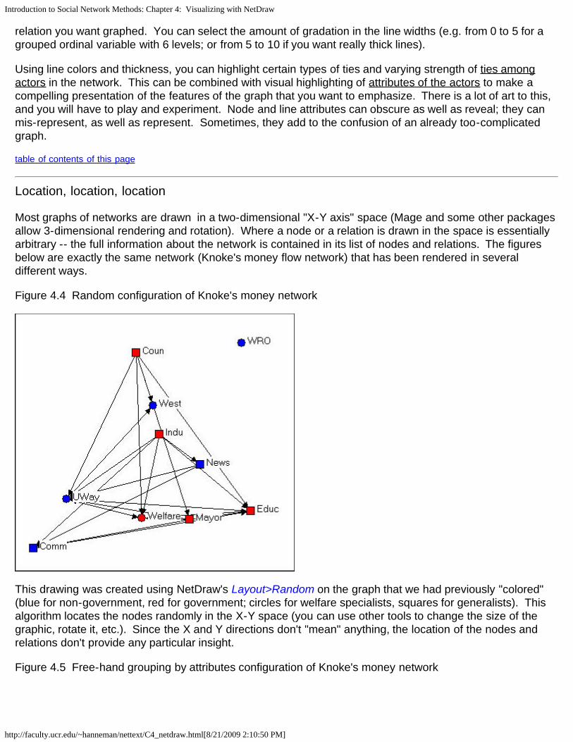
Introduction to Social Network Methods: Chapter 4: Visualizing with NetDraw
http://faculty.ucr.edu/~hanneman/nettext/C4_netdraw.html[8/21/2009 2:10:50 PM]
relation you want graphed. You can select the amount of gradation in the line widths (e.g. from 0 to 5 for agrouped ordinal variable with 6 levels; or from 5 to 10 if you want really thick lines).
Using line colors and thickness, you can highlight certain types of ties and varying strength of ties amongactors in the network. This can be combined with visual highlighting of attributes of the actors to make acompelling presentation of the features of the graph that you want to emphasize. There is a lot of art to this,and you will have to play and experiment. Node and line attributes can obscure as well as reveal; they canmis-represent, as well as represent. Sometimes, they add to the confusion of an already too-complicatedgraph.
table of contents of this page
Location, location, location
Most graphs of networks are drawn in a two-dimensional "X-Y axis" space (Mage and some other packagesallow 3-dimensional rendering and rotation). Where a node or a relation is drawn in the space is essentiallyarbitrary -- the full information about the network is contained in its list of nodes and relations. The figuresbelow are exactly the same network (Knoke's money flow network) that has been rendered in severaldifferent ways.
Figure 4.4 Random configuration of Knoke's money network
This drawing was created using NetDraw's Layout>Random on the graph that we had previously "colored"(blue for non-government, red for government; circles for welfare specialists, squares for generalists). Thisalgorithm locates the nodes randomly in the X-Y space (you can use other tools to change the size of thegraphic, rotate it, etc.). Since the X and Y directions don't "mean" anything, the location of the nodes andrelations don't provide any particular insight.
Figure 4.5 Free-hand grouping by attributes configuration of Knoke's money network

Introduction to Social Network Methods: Chapter 4: Visualizing with NetDraw
http://faculty.ucr.edu/~hanneman/nettext/C4_netdraw.html[8/21/2009 2:10:50 PM]
In figure 4.5, we've used the "drag and drop" method ("grab" a node with the cursor, and drag it to a newlocation) to relocate the nodes so that organizations that share the same combinations of attributes arelocated in different quadrants of the graph. Since we had hypothesized that organizations of like "kind"would have higher rates of connection, this is a useful (but still arbitrary) way to locate the points. If thehypothesis were strongly supported (and its not) most of the arrows would be located within each the fourquadrants, and there would be few arrows between quadrants. NetDraw has a built-in tool that allows theuser to assign the X and Y dimensions of the graph to scores on attributes (either categorical or continuous):Layout>Attributes as Coordinates, and then select attributes to be assigned to X or Y or both. This can be avery useful tool for exploring how patterns of ties differ within and between "partitions" (or types of nodes).
Figure 4.6 Circle configuration of Knoke's money network
Figure 4.6 shows the same graph using Layout>Circle, and selecting the "generalist-specialist" (i.e. thecircle or square node type) as the organizing criterion. Circle graphs are commonly used to visualize whichnodes are most highly connected. The nodes are located at equal distances around a circle, and nodes thatare highly connected are very easy to quickly locate (e.g. UWay, Educ) because of the density of lines.

Introduction to Social Network Methods: Chapter 4: Visualizing with NetDraw
http://faculty.ucr.edu/~hanneman/nettext/C4_netdraw.html[8/21/2009 2:10:50 PM]
When nodes sharing the same attribute are located together in a segment of the circle, the density of tieswithin and between types is also quite apparent.
In each of the different layouts we've discussed so far, the distances between the nodes are arbitrary, andcan't be interpreted in any meaningful way as "closeness" of the actors. And, the "directions" X and Y haveno meaning -- we could rotate any of the graphs any amount, and it would not change a thing about ourinterpretation. There are several other commonly used graphic layouts that do try to make the distancesand/or directions of locations among the actors somewhat more meaningful.
Figure 4.7 Non-metric multi-dimensional scaling configuration of Knoke's money network
Figure 4.7 was generated using the Layout>Graph Theoretic Layout>MDS tool of NetDraw. MDS stands for(non-metric, in this case) "Multi-Dimensional Scaling." MDS is a family of techniques that is used (in networkanalysis) to assign locations to nodes in multi-dimensional space (in the case of the drawing, a 2-dimensional space) such that nodes that are "more similar" are closer together. There are many reasonabledefinitions of what it means for two nodes to be "similar." In this example, two nodes are "similar" to theextent that they have similar shortest paths (geodesic distances) to all other nodes. There are many, manyways of doing MDS, but the default tools chosen in NetDraw can often generate meaningful renderings ofgraphs that provide insights. NetDraw has several built-in algorithms for generating coordinates based onsimilarity (metric and non-metric two-dimensional scaling, and principle components analysis).
One very important difference between figure 4.7 and the earlier graphs is that the distances between thenodes is interpretable. The "Welfare" and "Mayor" nodes are very similar in their geodesic distances fromother actors. "West" and "Educ" have very different patterns of ties to the other nodes.
The other important difference between figure 4.7 and the earlier graphs is that direction may be meaningful. Notice that there is a cluster of nodes at the left (News, Indu, Comm) that are all pretty much not welfareorganizations themselves, while the nodes at the right are (generally) more directly involved in welfareservice provision. The upper left-hand quadrant contains mostly "blue" nodes, while the lower right quadrantcontains mostly "red" ones -- so one "direction" might be interpreted as "non-government/government."
Let me emphasize that different applications of MDS (and other scaling tools) to different definitions of what itmeans for nodes to be "similar" can generate wildly different looking graphs. These are (almost always)exploratory techniques, and there is (usually) no single "correct" interpretation. But, a graphic that uses bothdistance and direction to summarize something about the structure of the network can provide considerable
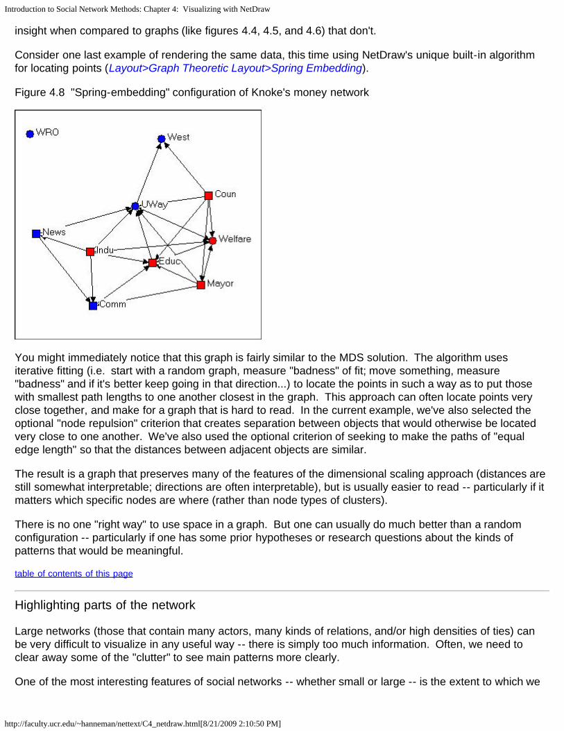
Introduction to Social Network Methods: Chapter 4: Visualizing with NetDraw
http://faculty.ucr.edu/~hanneman/nettext/C4_netdraw.html[8/21/2009 2:10:50 PM]
insight when compared to graphs (like figures 4.4, 4.5, and 4.6) that don't.
Consider one last example of rendering the same data, this time using NetDraw's unique built-in algorithmfor locating points (Layout>Graph Theoretic Layout>Spring Embedding).
Figure 4.8 "Spring-embedding" configuration of Knoke's money network
You might immediately notice that this graph is fairly similar to the MDS solution. The algorithm usesiterative fitting (i.e. start with a random graph, measure "badness" of fit; move something, measure"badness" and if it's better keep going in that direction...) to locate the points in such a way as to put thosewith smallest path lengths to one another closest in the graph. This approach can often locate points veryclose together, and make for a graph that is hard to read. In the current example, we've also selected theoptional "node repulsion" criterion that creates separation between objects that would otherwise be locatedvery close to one another. We've also used the optional criterion of seeking to make the paths of "equaledge length" so that the distances between adjacent objects are similar.
The result is a graph that preserves many of the features of the dimensional scaling approach (distances arestill somewhat interpretable; directions are often interpretable), but is usually easier to read -- particularly if itmatters which specific nodes are where (rather than node types of clusters).
There is no one "right way" to use space in a graph. But one can usually do much better than a randomconfiguration -- particularly if one has some prior hypotheses or research questions about the kinds ofpatterns that would be meaningful.
table of contents of this page
Highlighting parts of the network
Large networks (those that contain many actors, many kinds of relations, and/or high densities of ties) canbe very difficult to visualize in any useful way -- there is simply too much information. Often, we need toclear away some of the "clutter" to see main patterns more clearly.
One of the most interesting features of social networks -- whether small or large -- is the extent to which we

Introduction to Social Network Methods: Chapter 4: Visualizing with NetDraw
http://faculty.ucr.edu/~hanneman/nettext/C4_netdraw.html[8/21/2009 2:10:50 PM]
can locate "local sub-structures." We will discuss this topic a good bit more in a later chapter. Highlighting orfocusing attention on sub-sets of nodes in a drawing can be a powerful tool for visualizing sub-structures.
In this section, we will briefly outline some approaches to rendering network drawings that can help tosimplify complex diagrams and locate interesting sub-graphs (i.e. collections of nodes and their connections).
Clearing away the underbrush
Social structures can be composed of multiple relations. Bob, Carol, Ted, and Alice in our earlier exampleare a multi-plex structure of people connected by both friendship and by spousal ties. Graphs that display allof the connections among a set of nodes can be very useful for understanding how actors are tied together --but they can also get so complicated and dense that it is difficult to see any patterns. There are a coupleapproaches that can help.
One approach is to combine multiple relations into an index. For example, one could combine theinformation on friendship and spousal ties using an "and" rule: if two nodes have both a friendship andspousal tie, then they have a tie - otherwise they do not (i.e. if they have no tie, or only one type of tie). Alternatively, we could create an index that records a tie when there is either a friendship tie or a spousal tie. If we had measured relations with values, rather than simple presence-absence, multiple relations could becombined by addition, subtraction, multiplication, division, averaging, or other methods. UCINET has toolsfor these kinds of operations, that are located at: Transform>matrix operations>withindataset>aggregations.
The other approach is to simplify the data a bit. NetDraw has some tools that can be of some help.
Rather than examining the information on multiple kinds of ties in one diagram, one can look at them one ata time, or in combination. If the data have been stored as a UCINET or NetDraw data file with multiplerelations, then the Options>View>Relations Box opens a dialog box that lets you select which relations youwant to display. Suppose that we had a data set in which we had recorded the friendship ties among anumber of people at intervals over a period of time. By first displaying the first time point, and then addingsubsequent time point, we can visualize the evolution of the friendship structure.
It isn't unusual for some of the nodes in a graph of a social network to not be connected to the others at all. Nodes that aren't connected are called "isolates." Some nodes may be connected to the network by a singletie. These nodes sort of "dangle" from the diagram; they are called "pendants." One way of simplifyinggraphs is to hide isolates and/or pendants to reduce visual clutter. Of course, this does mis-represent thestructure, but it may allow us to focus more attention where most of the action is. NetDraw has both button-bar tools and a menu item (Analysis>Isolates) to hide these less-connected nodes.
Finding and visualizing local sub-structures
One of the common questions in network analysis is whether a graph displays various kinds of "sub-structures." For example, a "clique" is a sub-structure that is defined as a set of nodes where every elementof the set is connected to every other member. A network that has no cliques might be a very different placethan a network that has many small cliques, or one that has one clique and many nodes that are not part ofthe clique. We'll take a closer look at UCINET tools for identifying sub-structures in a later chapter.
NetDraw has built-in a number of tools for identifying sub-structures, and automatically coloring the graph toidentify them visually.
Analysis>components locates the parts of graph that are completely disconnected from one another, andcolors each set of nodes (i.e. each component). In our Bob-Carol-Ted-Alice example, the entire graph is onecomponent, because all the actors are connected. In the welfare bureaucracies example, there are two
Introduction to Social Network Methods: Chapter 4: Visualizing with NetDraw
http://faculty.ucr.edu/~hanneman/nettext/C4_netdraw.html[8/21/2009 2:10:50 PM]
components, one composed of only WRO (which does not receive ties from any other organization) and theother composed of the other nine nodes. In NetDraw, executing this command also creates a variable in thedatabase of node attributes -- as do all the other commands discussed here. These attributes can then beused for selecting cases, changing color, shape, and size, etc.
Analysis>Blocks and Cutpoints locates parts of the graph that would become disconnected components ifeither one node or one relation were removed (the blocks are the resulting components; the cutpoint is thenode that would, if removed, create the dis-connect). NetDraw graphs these sub-structures, and saves theinformation in the node-attribute database.
Analysis>K-cores locates parts of the graph that form sub-groups such that each member of a sub-group isconnected to N-K of the other members. That is, groups are the largest structures in which all members areconnected to all but some number (K) of other members. A "clique" is a group like this where all membersare connected to all other members; "fuzzier" or "looser" groups are created by increasing "K." NetDrawidentifies the K-cores that are created by different levels of K, and provides colored graphs and data-baseentries.
Analysis>Subgroups>block based. Sorry, but I don't know what this algorithm does! Most likely, it createssub-structures that would become components with differing amounts of nodes/relations removed.
Analysis>Subgroups>Hierarchical Clustering of Geodesic Distances. The geodesic distance between twonodes is the length of the shortest path between them. A hierarchical clustering of distances produces atree-like diagram in which the two nodes that are most similar in their profile of distances to all other pointsare joined into a cluster; the process is then repeated over and over until all nodes are joined. The resultinggraphic is one way of understanding which nodes are most similar to one another, and how the nodes maybe classified into "types" based on their patterns of connection to other nodes. The graph is colored torepresent the clusters, and database information is stored about the cluster memberships at various levels ofaggregation. A hierarchical clustering can be very interesting in understanding which groups are morehomogeneous (those that group together at early stages in the clustering) than others; moving up theclustering tree diagram, we can see a sort of a "contour map" of the similarity of nodes.
Analysis>Subgroups>Factions (select number). A "faction" is a part of a graph in which the nodes are moretightly connected to one another than they are to members of other "factions." This is quite an intuitivelyappealing idea of local clustering or sub-structure (though, as you can see, only one such idea). NetDrawasks you how many factions you would like to find (always explore various reasonable possibilities!). Thealgorithm then forms the number of groups that you desire by seeking to maximize connection within, andminimize connection between the groups. Points are colored, and the information about which nodes fall inwhich partitions (i.e. which cases are in which factions) is saved to the node attributes database.
Analysis>Subgroups>Newman-Girvan. This is another numerical algorithm that seeks to create clusters ofnodes that are closely connected within, and less connected between clusters. The approach is that of"block modeling." Rows and columns are moved to try to create "blocks" where all connections within ablock are present, and all connections between blocks are absent. This algorithm will usually produceresults similar to the factions algorithm. Importantly, though, the Newman-Girvan algorithm also producesmeasures of goodness-of-fit of the configuration for two blocks, three blocks, etc. This allows you to getsome sense of what division into blocks is optimal for your needs (there isn't one "right" answer).
Ego Networks (neighborhoods)
A very useful way of understanding complicated network graphs is to see how they arise from the localconnections of individual actors. The network formed by selecting a node, including all actors that areconnected to that node, and all the connections among those other actors is called the "ego network" or (1-
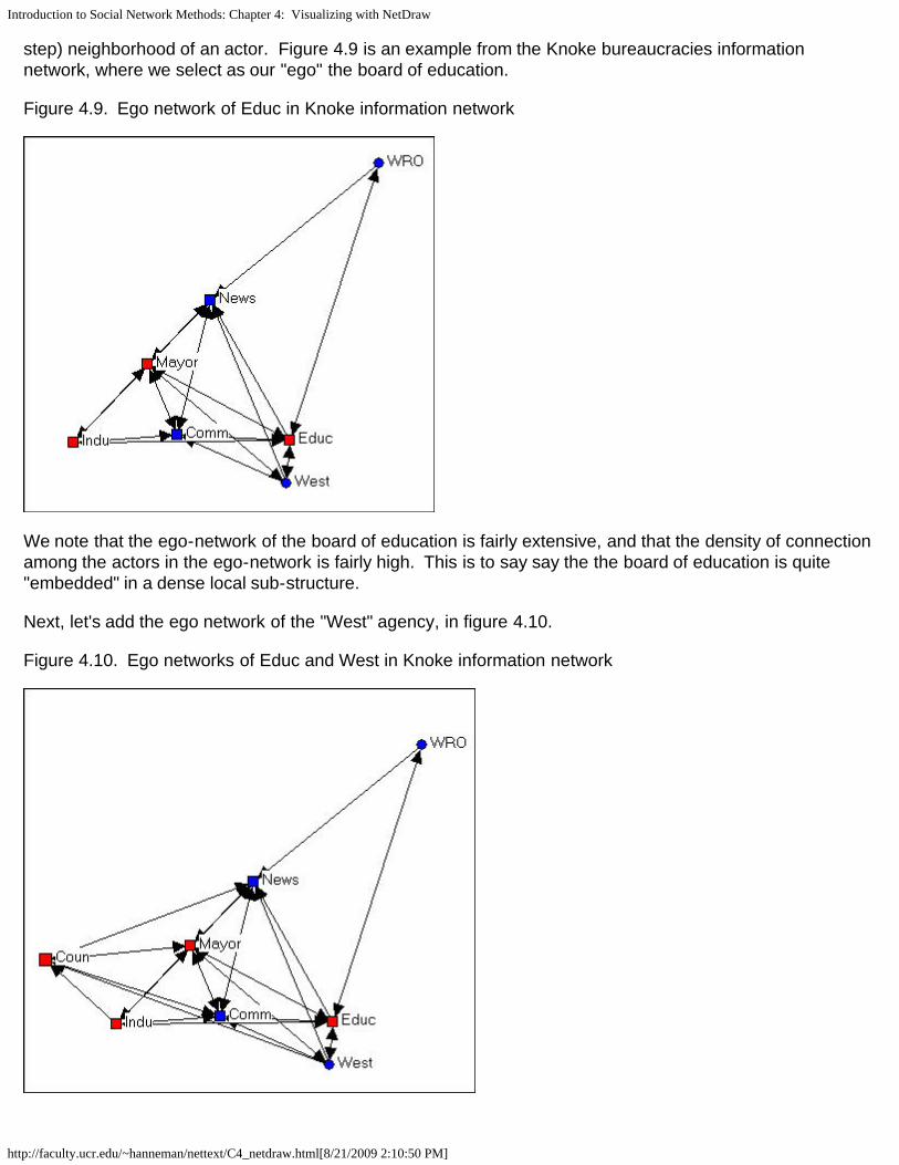
Introduction to Social Network Methods: Chapter 4: Visualizing with NetDraw
http://faculty.ucr.edu/~hanneman/nettext/C4_netdraw.html[8/21/2009 2:10:50 PM]
step) neighborhood of an actor. Figure 4.9 is an example from the Knoke bureaucracies informationnetwork, where we select as our "ego" the board of education.
Figure 4.9. Ego network of Educ in Knoke information network
We note that the ego-network of the board of education is fairly extensive, and that the density of connectionamong the actors in the ego-network is fairly high. This is to say say the the board of education is quite"embedded" in a dense local sub-structure.
Next, let's add the ego network of the "West" agency, in figure 4.10.
Figure 4.10. Ego networks of Educ and West in Knoke information network

Introduction to Social Network Methods: Chapter 4: Visualizing with NetDraw
http://faculty.ucr.edu/~hanneman/nettext/C4_netdraw.html[8/21/2009 2:10:50 PM]
The two ego networks combined result in a fully connected structure. We note that one connection betweenEduc and Coun is mediated by West.
One can often gain considerable insight about complicated networks by "building" them starting with oneactor and adding others. Or, one can begin with the whole network, and see what happens as individual'sego networks are removed.
The network of each individual actor may also be of considerable interest. Who's most connected? Howdense are the neighborhoods of particular actors?
NetDraw has useful tools for visualizing and working with ego-networks. The Layout>Egonet commandpresents a dialog box that lets you select which ego's networks are to be displayed. You can start with all theactors and delete; or start with focal actors and build up the full network.
table of contents of this page
A few hints on data handling with NetDraw
Input
There are several ways to get data into NetDraw. Probably the simplest is to import data from UCINET orPajek. The File>Open command lets you read a UCINET text (DL) file (discussed elsewhere), and existingUCINET dataset, or a Pajek dataset. This menu also is used to access data that have been stored in thenative data format of the NetDraw program (.VNA format). Once the data has been imported with the Opencommand, the node and line attribute editors of NetDraw can be used to create a diagram that can be savedwith colors, shapes, locations, etc.
A second method is to build a dataset within NetDraw itself. Begin by creating a random network(File>Random). This creates an arbitrary network of 20 nodes. You can then use the node attributes editor(Transform>Node Attribute editor) and the link editor (Transform>Link Editor) to modify the nodes (and addor delete nodes) and their attributes; and to create connections among nodes. This is great for small, simplenetworks; for more complicated data, it's best to create the basic data set elsewhere and import it.
The third method is to use an external editor to create a NetDraw dataset (a .vna file) directly. This file is aplain ascii text file (if you use a word processor, be sure to save as ascii text). The contents of the file ispretty simple, and is discussed in the brief tutorial to NetDraw. Here is part of the file for the Knoke data,after we have created some of the diagrams we've seen.
*Node data"ID", "General", "Size", "Govt" "1" "1" "3" "1" "2" "1" "2" "0".. "9" "0" "2" "1" "10" "0" "1" "0"*Node propertiesID x y color shape size shortlabel labelsize labelcolor active"1" 51 476 255 2 16 "Coun" 11 0 TRUE"2" 451 648 16711680 2 11 "Comm" 11 0 TRUE.."9" 348 54 255 1 11 "Welfare" 11 0 TRUE"10" 744 801 16711680 1 6 "West" 11 0 TRUE*Tie dataFROM TO "KNOKI" "KNOKM"

Introduction to Social Network Methods: Chapter 4: Visualizing with NetDraw
http://faculty.ucr.edu/~hanneman/nettext/C4_netdraw.html[8/21/2009 2:10:50 PM]
"1" "2" 1 0"1" "5" 1 1.."9" "3" 0 1"9" "8" 0 1*Tie propertiesFROM TO color size active"1" "2" 0 1 TRUE"1" "5" 0 1 TRUE.."9" "3" 0 1 FALSE"9" "8" 0 1 FALSE
There are four sections of code here (not all are needed, but the *node data and *tie data are, to define thenetwork structure). *Node data lists variables describing the nodes. An ID variable is necessary, the othervariables in the example describe attributes of each node. The (optional) *Node properties section lists thevariables, and gives values for ID, location on the diagram (X and Y coordinates from the upper left corner),shape, size, color, etc. Usually, one will not create this code; rather you input the data, use NetDraw tocreate a diagram, and save the result as a file -- and this section (and the *Tie properties) is created for you.
The *Tie data section is necessary to define the connections among the nodes. There is one data line foreach relation in the graph. Each data line is described by its origin and destination, and value. Here. sincethere are two relations, "KNOKI" and "KNOKM" there are two values -- each of which happens, in ourexample, to be binary (but they could be valued).
The *Tie properties section is probably best created by using NetDraw and saving the resulting file. Each tieis identified by origin and destination, and its color and size are set. Here, certain ties are not to be visible inthe drawing (the "active" property is set to "FALSE").
Output
When you are working with NetDraw, it is a good idea to save a copy of your work in the format (.vna, above)that is native to the program (File>Save Data As>Vna). This format keeps all of the information about yourdiagram (what's visible and not, node and line attributes, locations) so that you can re-open the diagramlooking exactly as you left it.
You may also want to save datasets created with NetDraw to other program's formats. You won't be able tosave all of the information about node and line properties and locations, but you can save the basic network(what are the nodes, which is connected to which) and node attributes. File>Save Data As>Pajek lets yousave the network, partitions of it (which record attributes), and clusterings in Pajek format. File>Save DataAs>UCINET lets you save the basic network information for binary or valued networks (UCINET needs toknow which) and attributes (which are stored in a separate file in UCINET).
The whole point of making more interesting drawings of graphs, of course, is to be able to use them toillustrate your ideas. There are several possibilities.
Screen capture programs (I used SnagIT) can take pictures of your graphics that can be then saved in anynumber of formats, and edited further by external graphics editors (perhaps to add titles, annotations, andother highlights).
File>print, of course, does just that.
File>Save Diagram As let's you save your diagram in three of the most common graphics formats (Windows

Introduction to Social Network Methods: Chapter 4: Visualizing with NetDraw
http://faculty.ucr.edu/~hanneman/nettext/C4_netdraw.html[8/21/2009 2:10:50 PM]
Metafile, bitmap BMP, or JPEG). Once saved, these file formats can be further edited with graphics editingprograms to be inserted into web or hard-copy documents.
table of contents of this page
Conclusions
A lot of the work that we do with social networks is primarily descriptive and/or exploratory, rather thanconfirmatory hypothesis testing. Using some of the tools described in this chapter can be particularly helpfulbecause they may let you see patterns that you might not otherwise have seen. The tools can be used toexplore tentative empirical generalizations and provide crude first examinations of hypotheses about patternsthat may be present in the data.
Some of the tools are also very helpful for dealing with the complexity of social network data, which mayinvolve many actors, many ties, and several types of ties. Hiding, highlighting, and locating parts of the datacan be a big help in making sense of the data. In some cases (like ego networks and the evolution ofnetworks over time) hiding and revealing parts of the data are critical to understanding and describing theconstruction and evolution of the social structures.
Finally, working with drawings can be a lot of fun, and a bit of an outlet for your creative side. A really goodgraphic can also be far more effective in sharing your insights than any number of words.
table of contents of this pagetable of contents of the textbook
Introduction to Social Network Methods; Chapter 5: Using Matrices
http://faculty.ucr.edu/~hanneman/nettext/C5_%20Matrices.html[8/21/2009 2:11:17 PM]
Introduction to social network methods
5. Using matrices to represent social relations
This page is part of an on-line text by Robert A. Hanneman (Department of Sociology, University of California, Riverside) and MarkRiddle (Department of Sociology, University of Northern Colorado). Feel free to use and distribute this textbook, with citation. Yourcomments and suggestions are very welcome. Send me e-mail.
Contents of this chapter:
What is a matrix?The "adjacency" matrixMatrix permutation, blocks, and imagesDoing mathematical operations on matricesTransposing a matrix
Taking the inverse of a matrixMatrix addition and matrix subtractionMatrix multiplication and Boolean matrix multiplication
SummaryStudy questions
Introduction
Graphs are very useful ways of presenting information about social networks. However, when there aremany actors and/or many kinds of relations, they can become so visually complicated that it is very difficult tosee patterns. It is also possible to represent information about social networks in the form of matrices.Representing the information in this way also allows the application of mathematical and computer tools tosummarize and find patterns. Social network analysts use matrices in a number of different ways. So,understanding a few basic things about matrices from mathematics is necessary. We'll go over just a fewbasics here that cover most of what you need to know to understand what social network analysts are doing.For those who want to know more, there are a number of good introductory books on matrix algebra forsocial scientists.
table of contents
What is a matrix?
To start with, a matrix is nothing more than a rectangular arrangement of a set of elements (actually, it's a bitmore complicated than that, but we will return to matrices of more than two dimensions in a little bit).Rectangles have sizes that are described by the number of rows of elements and columns of elements thatthey contain. A "3 by 6" matrix has three rows and six columns; an "I by j" matrix has I rows and j columns. Amatrix that has only one row is called a "row vector." A matrix that has only one column is called a "columnvector.
Figure 5.1 shows a two-by-four matrix. Figure 5.2 shows a four by two matrix. Just for the moment, ignorethe contents of the cells (e.g. 1,1).
Figure 5.1. Example of a "two-by-four" matrix

Introduction to Social Network Methods; Chapter 5: Using Matrices
http://faculty.ucr.edu/~hanneman/nettext/C5_%20Matrices.html[8/21/2009 2:11:17 PM]
1,1 1,2 1,3 1,42,1 2,2 2,3 2,4
Figure 5.2. Example of at "four-by-two" matrix
1,1 1,22,1 2,23,1 3,24,1 4,2
The elements (cells) of a matrix are identified by their "addresses." Element 1,1 is the entry in the first rowand first column; element 13,2 is in the 13th row and is the second element of that row. The cell addresseshave been entered as matrix elements in the two examples above.
Matrices are often represented as arrays of elements surrounded by vertical lines at their left and right, orsquare brackets at the left and right. In web pages it's easier to use "tables" to represent matrices. Matricescan be given names; these names are usually presented as capital bold-faced letters. Social scientists usingmatrices to represent social networks often dispense with the mathematical conventions, and simply showtheir data as an array of labeled rows and columns. The labels are not really part of the matrix, but aresimply for clarity of presentation. The matrix in figure 5.3 for example, is a 4 by 4 matrix, with additionallabels.
Figure 5.3. Four-by-four matrix with additional row and column labels
A B C DA --- 1 0 0B 1 --- 1 0C 1 1 --- 1D 0 0 1 ---
The matrices used in social network analysis are frequently "square." That is, they contain the same numberof rows and columns. But "rectangular" matrices are also used, as are row and column vectors. The sameconventions apply to all these variations.
Occasionally, social network analysts will use a "3-dimensional" matrix. A three dimensional matrix hasrows, columns, and "levels" or "slices." Each "slice" has the same rows and columns as each other slice. UCINET thinks about these more complicated 3-dimensional arrays of data as a collection of two-dimensional matrices.
table of contents
The "adjacency" matrix
The most common form of matrix in social network analysis is a very simple square matrix with as many rowsand columns as there are actors in our data set. The "elements" or scores in the cells of the matrix recordinformation about the ties between each pair of actors.
The simplest and most common matrix is binary. That is, if a tie is present, a one is entered in a cell; if there

Introduction to Social Network Methods; Chapter 5: Using Matrices
http://faculty.ucr.edu/~hanneman/nettext/C5_%20Matrices.html[8/21/2009 2:11:17 PM]
is no tie, a zero is entered. This kind of a matrix is the starting point for almost all network analysis, and iscalled an "adjacency matrix" because it represents who is next to, or adjacent to whom in the "social space"mapped by the relations that we have measured.
An adjacency matrix may be "symmetric" or "asymmetric." Social distance can be either symmetric orasymmetric. If Bob and Carol are "friends" they share a "bonded tie" and the entry in the Xi,j cell will be thesame as the entry in the Xj,i cell.
But social distance can be a funny (non-Euclidean) thing. Bob may feel close to Carol, but Carol may notfeel the same way about Bob. In this case, the element showing Bob's relationship to Carol would be scored"1," while the element showing Carol's relation to Bob would be scored "0." That is, in an "asymmetric"matrix, Xi,j is not necessarily equal to Xj,i.
By convention, in a directed (i.e. asymmetric) matrix, the sender of a tie is the row and the target of the tie isthe column. Let's look at a simple example. The directed graph of friendship choices among Bob, Carol, Ted,and Alice is shown in figure 5.4.
Figure 5.4 Bob, Carol, Ted, and Alice
We can since the ties are measured at the nominal level (that is, the data are binary choice data), we canrepresent the same information in a matrix that looks like:
Figure 5.5. Asymmetric adjacency matrix of the graph shown in figure 5.4.
Bob Carol Ted AliceBob --- 1 1 0Carol 0 --- 1 0Ted 1 1 --- 1Alice 0 0 1 ---
Remember that the rows represent the source of directed ties, and the columns the targets; Bob choosesCarol here, but Carol does not choose Bob. This is an example of an "asymmetric" matrix that representsdirected ties (ties that go from a source to a receiver). That is, the element i,j does not necessarily equal theelement j,i. If the ties that we were representing in our matrix were "bonded-ties" (for example, tiesrepresenting the relation "is a business partner of" or "co-occurrence or co-presence," (e.g. where tiesrepresent a relation like: "serves on the same board of directors as") the matrix would necessarily besymmetric; that is element i,j would be equal to element j,i.
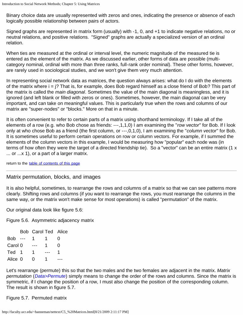
Introduction to Social Network Methods; Chapter 5: Using Matrices
http://faculty.ucr.edu/~hanneman/nettext/C5_%20Matrices.html[8/21/2009 2:11:17 PM]
Binary choice data are usually represented with zeros and ones, indicating the presence or absence of eachlogically possible relationship between pairs of actors.
Signed graphs are represented in matrix form (usually) with -1, 0, and +1 to indicate negative relations, no orneutral relations, and positive relations. "Signed" graphs are actually a specialized version of an ordinalrelation.
When ties are measured at the ordinal or interval level, the numeric magnitude of the measured tie isentered as the element of the matrix. As we discussed earlier, other forms of data are possible (multi-category nominal, ordinal with more than three ranks, full-rank order nominal). These other forms, however,are rarely used in sociological studies, and we won't give them very much attention.
In representing social network data as matrices, the question always arises: what do I do with the elementsof the matrix where i = j? That is, for example, does Bob regard himself as a close friend of Bob? This part ofthe matrix is called the main diagonal. Sometimes the value of the main diagonal is meaningless, and it isignored (and left blank or filled with zeros or ones). Sometimes, however, the main diagonal can be veryimportant, and can take on meaningful values. This is particularly true when the rows and columns of ourmatrix are "super-nodes" or "blocks." More on that in a minute.
It is often convenient to refer to certain parts of a matrix using shorthand terminology. If I take all of theelements of a row (e.g. who Bob chose as friends: ---,1,1,0) I am examining the "row vector" for Bob. If I lookonly at who chose Bob as a friend (the first column, or ---,0,1,0), I am examining the "column vector" for Bob.It is sometimes useful to perform certain operations on row or column vectors. For example, if I summed theelements of the column vectors in this example, I would be measuring how "popular" each node was (interms of how often they were the target of a directed friendship tie). So a "vector" can be an entire matrix (1 x... or ...x 1), or a part of a larger matrix.
return to the table of contents of this page
Matrix permutation, blocks, and images
It is also helpful, sometimes, to rearrange the rows and columns of a matrix so that we can see patterns moreclearly. Shifting rows and columns (if you want to rearrange the rows, you must rearrange the columns in thesame way, or the matrix won't make sense for most operations) is called "permutation" of the matrix.
Our original data look like figure 5.6:
Figure 5.6. Asymmetric adjacency matrix
Bob Carol Ted AliceBob --- 1 1 0Carol 0 --- 1 0Ted 1 1 --- 1Alice 0 0 1 ---
Let's rearrange (permute) this so that the two males and the two females are adjacent in the matrix. Matrixpermutation (Data>Permute) simply means to change the order of the rows and columns. Since the matrix issymmetric, if I change the position of a row, I must also change the position of the corresponding column. The result is shown in figure 5.7.
Figure 5.7. Permuted matrix

Introduction to Social Network Methods; Chapter 5: Using Matrices
http://faculty.ucr.edu/~hanneman/nettext/C5_%20Matrices.html[8/21/2009 2:11:17 PM]
Bob Ted Carol AliceBob --- 1 1 0Ted 1 --- 1 1Carol 0 1 --- 0Alice 0 1 0 ---
None of the elements have had their values changed by this operation or rearranging the rows and columns,we have just shifted things around. We've also highlighted some sections of the matrix. Each colored sectionis referred to as a block. Blocks are formed by passing dividing lines through the matrix (e.g. between Tedand Carol) rows and columns. Passing these dividing lines through the matrix is called partitioning the matrix.Here we have partitioned by the actor by their sex. Partitioning is also sometimes called "blocking thematrix," because partitioning produces blocks.
This kind of grouping of cells is often done in network analysis to understand how some sets of actors are"embedded" in social roles or in larger entities. Here, for example, we can see that all occupants of the socialrole "male" choose each other as friends; no females choose each other as friends, and that males are morelikely to choose females (3 out of 4 possibilities are selected) than females are to choose males (only 2 outof 4 possible choices). We have grouped the males together to create a "partition" or "super-node" or "socialrole" or "block." We often partition social network matrices in this way to identify and test ideas about howactors are "embedded" in social roles or other "contexts."
We might wish to dispense with the individual nodes altogether, and examine only the positions or roles. Ifwe calculate the proportion of all ties within a block that are present, we can create a block density matrix. Indoing this, we have ignored self-ties in figure 5.8.
Figure 5.8. Block density matrix
Male FemaleMale 1.00 0.75Female 0.50 0.00
We may wish to summarize the information still further by using block image or image matrix. If the density ina block is greater than some amount (we often use the average density for the whole matrix as a cut-offscore, in the current example the density is .58), we enter a "1" in a cell of the blocked matrix, and a "0"otherwise. This kind of simplification is called the "image" of the blocked matrix, as in figure 5.9.
Figure 5.9. Image matrix of sex blocked data, using overall mean density as the cut-off
Male FemaleMale 1 1Female 0 0
Images of blocked matrices are powerful tools for simplifying the presentation of complex patterns of data.Like any simplifying procedure, good judgment must be used in deciding how to block and what cut-offs touse to create images -- or we may lose important information.
UCINET includes tools that make permuting and blocking matrices rather easy.

Introduction to Social Network Methods; Chapter 5: Using Matrices
http://faculty.ucr.edu/~hanneman/nettext/C5_%20Matrices.html[8/21/2009 2:11:17 PM]
Transform>Block allows you to select a matrix to be blocked, a row and/or column partition, and a method forcalculating the entries in the resulting blocks.
To use this command, you need to first create separate files that describe the row partition and the columnpartition. These files are simply vectors (either one row, or one column) that identify which actors are to fallinto which partition. For example, if actors 1, 2, and 5 were to form group A, and actors 3 and 4 were to formgroup B, my column partition data set would read: 1 1 2 2 1. These partitions or blockings are simply regularUCINET data files with one row or one column.
The command asks for a method of summarizing the information within each block. You may take theaverage of the values in the block (if the data are binary, taking the average is the same thing as calculatingthe density), sum the values in the block, select the highest value or the lowest value, or select a measure ofthe amount of variation among the scores in the block -- either the sums of squares or the standarddeviation.
The command outputs two new matrices. The "PreImage" data set contains the original scores, butpermuted; the "Reduced image dataset" contains a new block matrix containing the block densities.
Transform>Collapse allows you to combine rows and/or columns by specifying (detailed instructions aregiven on the command window) which elements are to be combined, and how. We might select, forexample, to combine columns 1, 2, and 5, and rows 1, 2, and 5 by taking the average of the values (we couldalso select the maximum, minimum, or sum). The command creates a new matrix that has collapsed thedesired rows or columns using the summary operation you selected.
The data menu also gives you some tools for this kind of work:
Data>Permute allows you to re-arrange the rows and/or columns and/or matrices (if your data set containsmultiple matrices representing multiple relations, like the Knoke bureaucracies "information" and "money"relations). You simply specify the new order with a list. If I wanted to group rows 1, 2, and 5 to be new rows1, 2, and 3; and rows 3 and 4 to be new rows 4 and 5, I would enter 1 2 4 5 3.
Data>Sort re-arranges the rows, columns, or both of the matrix according to a criterion you select. If youdata are valued (i.e. represent tie strength) you might want to sort the rows and columns in ascending ordescending order (this could make sense for binary data, too). If you want a more complicated sort (say "allthe 3's first, then all the 1's, then all the 2's) you can use an external UCINET data file to specify this as avector (i.e. the data set would just be: 3 1 2).
Data>Transpose re-arranges the data in a way that is very commonly used in matrix algebra -- by taking the"transpose." A transpose is, very simply, switching the rows and columns of a matrix for one another.
table of contents
Doing mathematical operations on matrices
Representing the ties among actors as matrices can help us to see patterns by performing simplemanipulations like summing row vectors or partitioning the matrix into blocks. Social network analysts use anumber of other mathematical operations that can be performed on matrices for a variety of purposes (matrixaddition and subtraction, transposes, inverses, matrix multiplication, and some other more exotic stuff likedeterminants and eigenvalues). Without trying to teach you matrix algebra, it is useful to know at least a littlebit about some of these mathematical operations, and what they are used for in social network analysis.
UCINET has built-in functions for doing most matrix algebra functions. Look under the Tools>Matrix Algebra

Introduction to Social Network Methods; Chapter 5: Using Matrices
http://faculty.ucr.edu/~hanneman/nettext/C5_%20Matrices.html[8/21/2009 2:11:17 PM]
menu. If you do know some matrix algebra, you will find that this tool lets you do almost anything to matrixdata that you may desire. But, you do need to know what you are doing. The help screen for this commandshows how to identify the matrix or matrices that are to be manipulated, and the algorithms that can beapplied.
Transposing a matrix
This simply means to exchange the rows and columns so that i becomes j, and vice versa. If we take thetranspose of a directed adjacency matrix and examine its row vectors (you should know all this jargon bynow!), we are looking at the sources of ties directed at an actor. The degree of similarity between anadjacency matrix and the transpose of that matrix is one way of summarizing the degree of symmetry in thepattern of relations among actors. That is, the correlation between an adjacency matrix and the transpose ofthat matrix is a measure of the degree of reciprocity of ties (think about that assertion a bit). Reciprocity ofties can be a very important property of a social structure because it relates to both the balance and to thedegree and form of hierarchy in a network. This command is also available as Data>Transpose.
Taking the inverse of a matrix
This is a mathematical operation that finds a matrix which, when multiplied by the original matrix, yields anew matrix with ones in the main diagonal and zeros elsewhere (which is called an identity matrix). Withoutgoing any further into this, you can think of the inverse of a matrix as being sort of the "opposite of" theoriginal matrix. Matrix inverses are used mostly in calculating other things in social network analysis. Theyare sometimes interesting to study in themselves, however. It is sort of like looking at black lettering on whitepaper versus white lettering on black paper: sometimes you see different things. Inverses are calculated withTools>Matrix Algebra.
Matrix addition and matrix subtraction
These are the easiest of matrix mathematical operations. One simply adds together or subtracts eachcorresponding i,j element of the two (or more) matrices. Of course, the matrices that this is being done tohave to have the same numbers of I and j elements (this is called "conformable" to addition and subtraction)- and, the values of i and j have to be in the same order in each matrix.
Matrix addition and subtraction are most often used in network analysis when we are trying to simplify orreduce the complexity of multiplex (multiple relations recorded as separate matrices or slices) data to simplerforms. If I had a symmetric matrix that represented the tie "exchanges money" and another that representedthe relation "exchanges goods" I could add the two matrices to indicate the intensity of the exchangerelationship. Pairs with a score of zero would have no relationship, those with a "1" would be involved ineither barter or commodity exchange, and those with a "2" would have both barter and commodity exchangerelations. If I subtracted the "goods" exchange matrix from the "money exchange" matrix, a score of -1 wouldindicate pairs with a barter relationship; a score of zero would indicate either no relationship or a barter andcommodity tie; a score of +1 would indicate pairs with only a commodified exchange relationship. Fordifferent research questions, either or both approaches might be useful. Tools>Matrix Algebra are one wayof doing these sorts of data transformations.
Matrix multiplication and Boolean matrix multiplication
Matrix multiplication is a somewhat unusual operation, but can be very useful for the network analyst. Youwill have to be a bit patient here. First we need to show you how to do matrix multiplication and a fewimportant results (like what happens when you multiply an adjacency matrix times itself, or raise it to apower). Then, we will try to explain why this is useful.

Introduction to Social Network Methods; Chapter 5: Using Matrices
http://faculty.ucr.edu/~hanneman/nettext/C5_%20Matrices.html[8/21/2009 2:11:17 PM]
To multiply two matrices, they must be "conformable" to multiplication. This means that the number of rows inthe first matrix must equal the number of columns in the second. Usually network analysis uses adjacencymatrices, which are square, and hence, conformable for multiplication. Multiplying a matrix by itself (i.e.raising it to a power) and multiplying a square matrix by its transpose are obviously "conformable." Unlikeregular multiplication of individual numbers X*Y is not the same thing as Y*X in matrix multiplication -- theorder matters!
To multiply two matrices, begin in the upper left hand corner of the first matrix, and multiply every cell in thefirst row of the first matrix by the values in each cell of the first column of the second matrix, and sum theresults. Proceed through each cell in each row in the first matrix, multiplying by the column in the second. Toperform a Boolean matrix multiplication, proceed in the same fashion, but enter a zero in the cell if themultiplication product is zero, and one if it is not zero. An example helps. Suppose we wanted to multiply thetwo matrices in figure 5.10.
Figure 5.10. Two matrices to be multiplied.
0 12 34 5
times
6 7 89 10 11
The result is shown in figure 5.11.
Figure 5.11. Result of matrix multiplication.
(0*6)+(1*9) (0*7)+(1*10) (0*8)+(1*11)(2*6)+(3*9) (2*7)+(3*10) (2*8)+(3*11)(4*6)+(5*9) (4*7)+(5*10) (4*8)+(5*11)
The mathematical operation in itself doesn't interest us here (any number of programs can perform matrixmultiplication). But, the operation is useful when applied to an adjacency matrix. Consider our four friendsagain, in figure 5.12.
Figure 5.12. Directed graph of friendship relations among Bob, Carol, Ted, and Alice
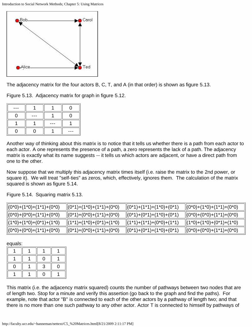
Introduction to Social Network Methods; Chapter 5: Using Matrices
http://faculty.ucr.edu/~hanneman/nettext/C5_%20Matrices.html[8/21/2009 2:11:17 PM]
The adjacency matrix for the four actors B, C, T, and A (in that order) is shown as figure 5.13.
Figure 5.13. Adjacency matrix for graph in figure 5.12.
--- 1 1 00 --- 1 01 1 --- 10 0 1 ---
Another way of thinking about this matrix is to notice that it tells us whether there is a path from each actor toeach actor. A one represents the presence of a path, a zero represents the lack of a path. The adjacencymatrix is exactly what its name suggests -- it tells us which actors are adjacent, or have a direct path fromone to the other.
Now suppose that we multiply this adjacency matrix times itself (i.e. raise the matrix to the 2nd power, orsquare it). We will treat "self-ties" as zeros, which, effectively, ignores them. The calculation of the matrixsquared is shown as figure 5.14.
Figure 5.14. Squaring matrix 5.13.
(0*0)+(1*0)+(1*1)+(0*0) (0*1)+(1*0)+(1*1)+(0*0) (0*1)+(1*1)+(1*0)+(0*1) (0*0)+(1*0)+(1*1)+(0*0)(0*0)+(0*0)+(1*1)+(0*0) (0*1)+(0*0)+(1*1)+(0*0) (0*1)+(0*1)+(1*0)+(0*1) (0*0)+(0*0)+(1*1)+(0*0)(1*0)+(1*0)+(0*1)+(1*0) (1*1)+(1*0)+(0*1)+(1*0) (1*1)+(1*1)+(0*0)+(1*1) (1*0)+(1*0)+(0*1)+(1*0)(0*0)+(0*0)+(1*1)+(0*0) (0*1)+(0*0)+(1*1)+(0*0) (0*1)+(0*1)+(1*0)+(0*1) (0*0)+(0*0)+(1*1)+(0*0)
equals:1 1 1 11 1 0 10 1 3 01 1 0 1
This matrix (i.e. the adjacency matrix squared) counts the number of pathways between two nodes that areof length two. Stop for a minute and verify this assertion (go back to the graph and find the paths). Forexample, note that actor "B" is connected to each of the other actors by a pathway of length two; and thatthere is no more than one such pathway to any other actor. Actor T is connected to himself by pathways of

Introduction to Social Network Methods; Chapter 5: Using Matrices
http://faculty.ucr.edu/~hanneman/nettext/C5_%20Matrices.html[8/21/2009 2:11:17 PM]
length two, three times. This is because actor T has reciprocal ties with each of the other three actors. Thereis no pathway of length two from T to B (although there is a pathway of length one).
So, the adjacency matrix tells us how many paths of length one are there from each actor to each otheractor. The adjacency matrix squared tells us how many pathways of length two are there from each actor toeach other actor. It is true (but we won't show it to you) that the adjacency matrix cubed counts the numberof pathways of length three from each actor to each other actor. And so on...
If we calculated the Boolean product, rather than the simple matrix product, the adjacency matrix squaredwould tell us whether there was a path of length two between two actors (not how many such paths therewere). If we took the Boolean squared matrix and multiplied it by the adjacency matrix using Booleanmultiplication, the result would tell us which actors were connected by one or more pathways of length three.And so on...
Now, finally: why should you care?
Some of the most fundamental properties of a social network have to do with how connected the actors areto one another. Networks that have few or weak connections, or where some actors are connected only bypathways of great length may display low solidarity, a tendency to fall apart, slow response to stimuli, and thelike. Networks that have more and stronger connections with shorter paths among actors may be morerobust and more able to respond quickly and effectively. Measuring the number and lengths of pathwaysamong the actors in a network allow us to index these important tendencies of whole networks.
Individual actor's positions in networks are also usefully described by the numbers and lengths of pathwaysthat they have to other actors. Actors who have many pathways to other actors may be more influential withregard to them. Actors who have short pathways to more other actors may me more influential or centralfigures. So, the number and lengths of pathways in a network are very important to understanding bothindividual's constraints and opportunities, and for understanding the behavior and potentials of the networkas a whole.
There are many measures of individual position and overall network structure that are based on whetherthere are pathways of given lengths between actors, the length of the shortest pathway between two actors,and the numbers of pathways between actors. Indeed, most of the basic measures of networks, measures ofcentrality and power, and measures of network groupings and substructures are based on looking at thenumbers and lengths of pathways among actors.
For most analyses, you won't have to manipulate matrices -- UCINET and other programs have already builtalgorithms that have the compute do these operations. Most of the computational work in network analysis isdone with matrix mathematics though, so in order to understand what is going on, it's useful to understandthe basics.
table of contents
Summary
Matrices are collections of elements into rows and columns. They are often used in network analysis torepresent the adjacency of each actor to each other actor in a network. An adjacency matrix is a squareactor-by-actor (i=j) matrix where the presence of pair wise ties are recorded as elements. The main diagonal,or "self-tie" of an adjacency matrix is often ignored in network analysis.
Sociograms, or graphs of networks can be represented in matrix form, and mathematical operations can thenbe performed to summarize the information in the graph. Vector operations, blocking and partitioning, and

Introduction to Social Network Methods; Chapter 5: Using Matrices
http://faculty.ucr.edu/~hanneman/nettext/C5_%20Matrices.html[8/21/2009 2:11:17 PM]
matrix mathematics (inverses, transposes, addition, subtraction, multiplication and Boolean multiplication),are mathematical operations that are sometimes helpful to let us see certain things about the patterns of tiesin social networks.
Social network data are often multiplex (i.e. there are multiple kinds of ties among the actors). Such data arerepresented as a series of matrices of the same dimension with the actors in the same position in eachmatrix. Many of the same tools that we can use for working with a single matrix (matrix addition andcorrelation, blocking, etc.) Are helpful for trying to summarize and see the patterns in multiplex data.
Once a pattern of social relations or ties among a set of actors has been represented in a formal way (graphsor matrices), we can define some important ideas about social structure in quite precise ways usingmathematics for the definitions. In the remainder of the book, we will look at how social network analystshave formally translated some of the core concepts that social scientists use to describe social structures.
table of contents
Review questions
1. A matrix is "3 by 2." How many columns does it have? How many rows?
2. Adjacency matrices are "square" matrices. Why?
3. There is a "1" in cell 3,2 of an adjacency matrix representing a sociogram. What does this tell us?
4. What does it mean to "permute" a matrix, and to "block" it?
Application questions
1. Think of the readings from the first part of the course. Did any studies present matrices? If they did, whatkinds of matrices were they (that is, what is the technical description of the kind of graph or matrix). Pick onearticle, and show what the data would look like, if represented in matrix form.
2. Think of some small group of which you are a member (maybe a club, or a set of friends, or people livingin the same apartment complex, etc.). What kinds of relations among them might tell us something about thesocial structures in this population? Try preparing a matrix to represent one of the kinds of relations youchose. Can you extend this matrix to also describe a second kind of relation? (e.g. one might start with "wholikes whom?" and add "who spends a lot of time with whom?").
3. Using the matrices you created in the previous question, does it make sense to leave the diagonal "blank,"or not, in your case? Try permuting your matrix, and blocking it.
4. Can you make an adjacency matrix to represent the "star" network? what about the "line" and "circle."Look at the ones and zeros in these matrices -- sometimes we can recognize the presence of certain kindsof social relations by these "digital" representations. What does a strict hierarchy look like? What does apopulation that is segregated into two groups look like?
table of contentstable of contents of the book

Introduction to Social Network Methods: Chapter 6: Working with Network Data
http://www.faculty.ucr.edu/~hanneman/nettext/C6_Working_with_data.html[8/21/2009 2:11:45 PM]
Introduction to social network methods
6. Working with network data
This page is part of an on-line text by Robert A. Hanneman (Department of Sociology, University of California, Riverside) and MarkRiddle (Department of Sociology, University of Northern Colorado). Feel free to use and distribute this textbook, with citation. Yourcomments and suggestions are very welcome. Send me e-mail.
Contents of this chapter
Introduction: Manipulating network data structuresMaking UCINET datasetsTransforming data valuesFile handling toolsSelecting sub-sets of the dataMaking new kinds of graphs from existing graphsConclusion
Introduction: Manipulating network data structures
This chapter is about the kinds of "data structures" that network analysts work with most frequently, andsome of the most common kinds of transformations and manipulations of these structures.
Data Structures
Most everyone reading this is very familiar with the kind of "data structure" that is used in many statisticalstudies. The rectangular array of data that we are used to seeing in SPSS, SAS, Excel, and other programsis a "structure" that is defined by its rows (which represent cases) and columns (which represent variables). An example is shown as figure 6.1.
Figure 6.1. Rectangular data array
ID Sex Age MarriedBob M 42 1Carol F 44 1Ted M 39 0Alice F 27 0
Earlier, we emphasized that the social network perspective leads us to focus our attention on the relationsbetween actors, more than on the attributes of actors. This approach often results in data that have adifferent "structure" in which both rows and columns refer to the same actors, and the cells report informationon one variable that describes variation (in the case of the example below, simple presence of absence of atie) in the relations between each pair of actors. An example is given as figure 6.2.
Figure 6.2. Square data structure for social network data
Friendship ties

Introduction to Social Network Methods: Chapter 6: Working with Network Data
http://www.faculty.ucr.edu/~hanneman/nettext/C6_Working_with_data.html[8/21/2009 2:11:45 PM]
Bob Carol Ted AliceBob --- 1 0 0Carol 0 --- 1 0Ted 1 1 --- 1Alice 0 0 1 ---
A "data structure" is simply the way in which information is recorded. These two examples are both two-dimensional (rows and columns). It is possible, for a data structure or data object to have more than twodimensions. For example, if we wanted to also record information about the network relations of who ismarried to whom, we would usually create another table of actors by actors (that is, the row and columnindexes would be the same), and record the presence or absence of marital ties. If we "stacked" the twotables together, we would have a 4 by 4 by 2 "data structure." Counts of the rows, columns, and matrices (or"slices") do not include the labeling or indexing information (i.e. it's not 5 x 5 x 3).
Social network analysis data structures:
Network analysts work with a variety of data structures. In this chapter, we'll look tools for creating andmanipulating the most common types.
One major "type" of data structure is the actor-by-actor matrix (like the friendship data above). This kind ofstructure is, by definition, a "two-dimensional," and "square" (the number of rows and columns are equal). The information in each cell provides information about the relation between a particular pair of actors.
The two-dimensional actor-by-actor matrix is very often expanded into a "third dimension" by adding "slices"that represent additional kinds of relations among the actors. For example, we might have an actor-by-actormatrix of Bob, Carol, Ted, and Alice that records the degree of "liking" directed from each to each. Inaddition, we might add a second "slice" that records the presence or absence of a kinship relation betweeneach pair. These kinds of 3-dimesional network data structures are "multi-plex." That is, they representmultiple relations among the same sets of actors. Some of the special issues in working with multi-plex dataare discussed in chapter 15.
The other major "type" of data structure that network analysts use looks a lot like the "rectangular data array"from conventional statistical work. The data structure consists of rows (representing actors) by columns(representing attributes of each actor -- what would be called "variables" in statistics). Such an array mightrecord just one attribute, in which case the data structure would be a "column vector." Or, such an arraymight record a number of attributes of each actor. Network analysts think of this kind of "rectangular" arrayof actors by attributes simply as a collection of vectors.
The "rectangular" data structure (called an "attribute" data set) is used in a number of ways in networkanalysis.
It can record attributes of each actor that we know from other sources (e.g. gender, age, etc.).It can record attributes of each actor that arise from their position in the network itself (e.g. the"between-ness centrality" score of each actor).It can record what part or sub-part of an network an actor falls in. For example, a column in an"attribute" data structure might consist of the letters "A" "B" and "C" to indicate which of three "factions"each actor was a member of. This is called a "partition."It can be used to tell UCINET how the actors in a matrix are to be re-arranged, or "permuted."
The "rectangular" data structure can also be used to record information about the relationships between twotypes of nodes (called bi-partite data). This use is so common and so important that it has a special name --

Introduction to Social Network Methods: Chapter 6: Working with Network Data
http://www.faculty.ucr.edu/~hanneman/nettext/C6_Working_with_data.html[8/21/2009 2:11:45 PM]
and "incidence" or an "affiliation" matrix. For example, the rows might be indexed by actors (e.g. Bob,Carol...); but, the columns might be the organizations that employ the actors (IBM, Sun, Microsoft...). Entriesin the cells indicate the presence or strength of the relation between an actor and an employer.
Incidence or affiliation data is particularly important in many social network analyses because it is "multi-level." Actors may be tied together because they are present in the same place, time, or category (that is,they are in the same "incident" to, or are "affiliated" with the same structure). But such data also show how"incidents" are tied together by the "co-presence" of actors. Incidence data involving two kinds of actors (bi-partite) data are very important in network analysis because they are often our best window into questions of"agency and structure" or "macro-micro linkages."
In this chapter we will describe some of the most common kinds of manipulations that social networkanalysts use in creating data structures, and changing their structures to meet the needs of particularresearch questions. Even though this chapter is going to be a bit long, it hardly covers all the possibilities. Different questions require different data structures. The examples and tools here will get you started.
table of contents
Making UCINET datasets
UCINET datasets are stored in a special (Pascal) format, but can be created and manipulated using bothUCINET's and other software tools (text editors and spreadsheets). Each UCINET dataset consists of twoseparate files that contain header information (e.g. myfile.##h) and the data lines (e.g. myfile.##d). Becauseof this somewhat unusual way of storing data, it is best to create data sets with the internal spreadsheeteditor or DL language tools, or to import text or spreadsheet files and save the results as UCINET files.
There are several ways of creating data files that UCINET can read.
The spreadsheet editor. UCINET has a built-in spreadsheet editor that can be used to enter case andvariable labels and data values (data>Spreadsheets>matrix). This editor allows you to specify the number ofrows and columns, and has the nice feature of being able to specify that a data set is symmetric. If we arerecording a data set where ties among actors are not directed, this feature saves half the data entry. Thereare also tools to fill the matrix with zeros (a common starting point for many data sets that have sparseconnections among actors), permuting rows, symmetrizing and dichotomizing (see discussions in thesections below), and copying row labels to the column labels (if the data are symmetric, you need only enterthe labels once).
The UCINET spreadsheet editor can import and export Excel spreadsheets, so you can use tools in bothprograms to full advantage. To import Excel to UCINET, be sure to save your spreadsheet as version 4 orearlier; the multi-sheet format of more recent Excel versions isn't supported in UCINET.
If you have a fairly small dataset, the UCINET spreadsheet editor is a good choice for making single matrixdatasets, which are automatically saved as UCINET files that can be used by other parts of the program.
Importing (and Exporting). Data sets can be moved from a number of other program's data file formats intoUCINET's. The Data>Import>... menu item supports import from NetDraw (VNA format), Pajek, Krackplot,and Negopy. It also supports importing raw ASCII text files, and files saved as Excel spreadsheets (version 4or earlier). So, if you started with a NetDraw drawing, for example, and saved the results as VNA, you mayimport this into UCINET for calculating network measures. I'm more comfortable with Excel than withUCINET's editor, so I usually make data sets in Excel, and import them.
When UCINET imports a file, it will produce a window with your results. Check to make sure they are

Introduction to Social Network Methods: Chapter 6: Working with Network Data
http://www.faculty.ucr.edu/~hanneman/nettext/C6_Working_with_data.html[8/21/2009 2:11:45 PM]
correct! When the import is performed, UCINET automatically saves the data files in UCINET format in thedefault directory.
It's often a good idea to set up a new directory for each project, and to set the default to this new directoryusing the file-cabinet icon on the toolbar, or File>Change default folder.
UCINET datasets can also be exported for use in other programs. Data>Export>... will produce Excel, rawASCII text, Pajek, Mage, Metis, and Krackplot files.
The DL language: If you've been looking at the UCINET Data menu as you read the preceding discussion,you may have noted that the program imports and exports "DL" files. DL (for "data language") is a verypowerful and (fairly) simple language that allows the creation of quite complex and large UCINET data setswith minimal data entry.
DL language files are plain ASCII text files that can be created with any editor (be sure to store the results asplain text). A quite complete reference guide is provided in UCINET (Help>Help Topics>DL).
The DL language can be a bit picky, and it does take a little effort to figure out how to do exactly what youwant to do with it. But, there are a number of circumstances where it is well worth the effort -- whencompared to using a spreadsheet. Particularly, if your data set consists of multiple matrices, and if the dataare fairly sparse, or if the data set has many rows and columns; then the DL file is the right way to go.
We won't explore the language in any detail here -- the help file is quite good. Figure 6.3 shows an exampleof a DL file that illustrates a few of the features.
Figure 6.3. Example DL language file
dl n=9, format=edgelist1labels: A,B,C,D,E,F,G,H,Idata: 1 1 1 1 2 1 1 6 1 . . . 8 7 1 9 9 1
The file begins with "dl" to indicate file type, and specification of the dimension of the data structure (thelanguage allows specification of number of rows, columns, and matrices). Labels for the nodes are given inthe "labels:" paragraph. The data are given in a "data:" paragraph.
The interesting thing in this example is the use of the format=edgelist1 command. This tells UCINET to readthe data lines in a way that is very efficient. The edgelist1 format is a set of rows, each one of whichidentifies two nodes and the value of the connection between them. In the resulting data set, all entries arezero, except those that have been specified. So, among our nine actors, there is a tie from actor 1 to actor 1,a tie from actor 1 to actor 2, a tie from actor 1 to actor 6, etc. Here, the matrix is binary -- the value of eachtie (the third entry on each line) is 1.
Another very useful format= method is nodelist1. In this format, each line of data consists of the name (ornumber) of an origin node, followed by all of the nodes to which it has a connection (this particularly format isfor zero/one data on the presence or absence of a connection). This approach then requires only one line ofdata for each actor. For example, a line in the data: section that read: 3 5 6 19 24 would indicate that actor

Introduction to Social Network Methods: Chapter 6: Working with Network Data
http://www.faculty.ucr.edu/~hanneman/nettext/C6_Working_with_data.html[8/21/2009 2:11:45 PM]
number 3 had a binary directed tie to actors 5, 6, 19, and 24.
These, and other methods available in DL allow the entry of very large and complex data sets with thegreatest efficiency and minimum typing. If you are facing a problem with many cases, connections, or kindsof connections, invest a little time in DL.
table of contents
Transforming data values
It is not at all unusual for the analyst to want to change the values that describe the relations between actors,or the values that describe the attributes of actors. Suppose the attribute "gender" had been entered into adata set using the values "1" and "2," and we wanted to change the attribute to be "Female" coded as "0"and "1." Or, suppose that we had recorded the strength of ties between companies by counting the numberof members of boards of directors that they had in common. But we then decide that we are only interestedin whether there are members in common or not. We need to change the coded values to be equal to "0" ifthere are no board members in common, and "1" if there are any (regardless of how many).
Just like statistical packages, UCINET has built-in tools that do some of the most common datatransformations.
Transform>Recode is a very flexible and general purpose tool for recoding values in any UCINET datastructure. its dialog box has two tabs: "Files" and "Recode."
In the files tab, you can browse for an input dataset, select which matrices in the set to recode (if there ismore than one), which rows and columns to recode (this is good if you are working on a collection of attributevectors, for example, and only want to recode selected ones), whether to recode the values on the diagonal,and the name of the output dataset.
In the recode tab, you specify what you want done by creating rules. For example, if I wanted to recode allvalues 1, 2, and 3 to be zero; and any values of 4, 5, and 6 to be one, I would create to rules. "Values from 1to 3 are recoded as 0" "Values from 4 to 6 are recoded as one." The rules are created by using simple built-in tools.
Almost any transformation in a data set of any complexity can be done with this tool. But, often there aresimpler ways to do certain tasks.
Transform>Reverse recodes the values of selected rows, columns, and matrices so that the highest value isnow the lowest, the lowest is now the highest, and all other values are linearly transformed. For example,the vector: 1 3 3 5 6 would become the vector 6 4 4 2 1.
If we've coded a relationship as "strength of tie" but want our results to be about "weakness of tie" a "reverse"transform would be helpful.
A common task in network analysis is to calculate the "similarity" or "distance" between two actors based ontheir relationships with other actors (more on this in the sections on equivalence, later). "Similarity" scorescan be "reversed" to become "dis-similarity;" "distance" scores can be "reversed" to be "nearness" scoreswith this tool.
Transform>Dichotomize is a tool that is useful for turning valued data into binary data. That is, if we havemeasured the strength of ties among actors (e.g. on a scale from 0 = no tie to 5 = strong tie), the"dichotomize" can be used to turn this into data that represent only the absence or presence of a tie (e.g.

Introduction to Social Network Methods: Chapter 6: Working with Network Data
http://www.faculty.ucr.edu/~hanneman/nettext/C6_Working_with_data.html[8/21/2009 2:11:45 PM]
zero or one).
Why would one ever want to do this? To convert an ordinal or interval measure of relation strength intosimple presence/absence may throw away considerable amounts of information. Many of the tools of socialnetwork analysis were developed for use with binary data only, and give misleading results (or none at all!)when applied to valued data. Many of the tools in UCINET that are designed for binary data will arbitrarilydichotomize interval or ordinal data in ways that might not be appropriate for your problem.
So, if your data are valued, but the tool you want to use requires binary data, you can turn your data intozero-one form by selecting a cut-off value (you will also have to select a "cut-off operator" and decide whatto do with the diagonal.
Suppose, for example, I'd measured tie strength on a scale from 0 to 3. I'd like to have the values 0 and 1treated as "0" and the values 2 and 3 treated as "1." I would select "greater than" as the cut-off operator, andselect a cut-off value of "2." The result would be a binary matrix of zeros (when the original scores were 0 or1) and ones (when the original scores were 2 or 3).
This tool can be particularly helpful when examining the values of many network measures. For example,the shortest distance between two actors ("geodesic distance") might be computed and saved in a file. Wemight then want to look at a map or image of the data at various levels of distance -- first, only display actorswho are adjacent (distance = 1), then actors who are one or two steps apart, etc. The "dichotomize" toolcould be used to create the necessary matrices.
Transform>Diagonal lets you modify the values of the ties of actors with themselves, or the "main diagonal"of square network data sets. The dialog box for this tool allows you to specify either a single value that is tobe entered for all the cells on the diagonal; or, a list of (comma separated) values for each of the diagonalcells (from actor one through the last listed actor).
For many network analyses, the values on the main diagonal are not very meaningful, and you may wish toset them all to zero or to one -- which are pretty common approaches. Many of the tools for calculatingnetwork measures in UCINET will automatically ignore the main diagonal, or ask you whether to include it ornot.
On some occasions, though, you may wish to be sure that ties of an actor with themselves are treated aspresent (e.g. set diagonal values to 1), or treated as absent (e.g. set diagonal values to zero).
Transform>Symmetrize is a tool that is used to turn "directed" or "asymmetric" network data into "un-directed" or "symmetric" data.
Many of the measures of network properties computed by UCINET are defined only for symmetric data (seethe help screens for information about this). If you ask to calculate a measure that is defined for onlysymmetric data, but your data are not symmetric, UCINET either will refuse to calculate a measure, or willsymmetrize the data for you.
But, there are a number of ways to symmetrize data, and you need to be sure that you choose an approachthat makes sense for your particular problem. The choices that are available in the Transform>Symmetrizetool are:
>Maximum looks at each cell in the upper part of the matrix and the corresponding cell in the lower part ofthe matrix (e.g. cell 2, 5 is compared to cell 5, 2), and enters the larger of the values found into both cells(e.g. 2, 5 and 5, 2 will now have the same output value). For example, suppose that we felt that the strengthof the tie between actor A and actor B was best represented as being the strongest of the ties between them(either A's tie to B, or B's tie to A, whichever was strongest).

Introduction to Social Network Methods: Chapter 6: Working with Network Data
http://www.faculty.ucr.edu/~hanneman/nettext/C6_Working_with_data.html[8/21/2009 2:11:45 PM]
>Minimum characterizes the strength of the symmetric tie between A and B as being the weaker of the tiesAB or BA. This corresponds to the "weakest link," and is a pretty common choice.
>Average characterizes the strength of the symmetric tie between A and B as the simple average of the tiesAB and BA. Honestly, I have trouble thinking of a case where this approach makes a lot of sense for socialrelations.
>Sum characterizes the strength of the symmetric tie between A and B as the sum of AB and BA. This doesmake some sense -- that all the tie strength be included, regardless of direction.
>Difference characterizes the strength of the symmetric tie between A and B as |AB - BA|. So, relationshipsthat are completely reciprocal end up with a value of zero; those what are completely asymmetric end up witha value equal to the stronger relation.
>Product characterizes the strength of the symmetric relation between A and B as the product of AB andBA. If reciprocity is necessary for us to regard a relationship as being "strong" then either "sum" or "product"might be a logical approach to symmetrizing.
>Division characterizes the strength of the symmetric relation between A and B as AB/BA. This approach"penalizes" relations that are equally reciprocated, and "rewards" relations that are strong in one direction,but not the other.
>Lower Half or >Upper Half uses the values in one half of the matrix for the other half. For example, thevalue of BA is set equal to whatever AB is. This transformation, though it may seem odd at first, is quitehelpful. If we are interested in focusing on the network properties of "senders" we would choose to set the lower half equal to the upper half (i.e. select Upper Half). If we wereinterested in the structure of tie receiving, we would set the upper half equal to the lower.
>Upper > Lower or >Upper < Lower (and similar functions available in the dialog box) compare the values incell AB and BA, and return one or the other based on the test function. If, for example, we had selectedUpper > Lower and AB = 3 and BA = 5, the function would select the value "5," because the upper value(AB) was not greater than the lower value (BA).
Transform>Normalize provides a number of tools for rescaling the scores in rows, in columns, or in bothdimensions of a matrix of valued relations. A simple example might be helpful.
Figure 6.4 shows some data (from the United Nations Commodity Trade database) on trade flows, valued indollars, of softwood lumber among 5 major Pacific Rim nations at c. 2000.
Figure 6.4. Value of softwood lumber exports among five nations
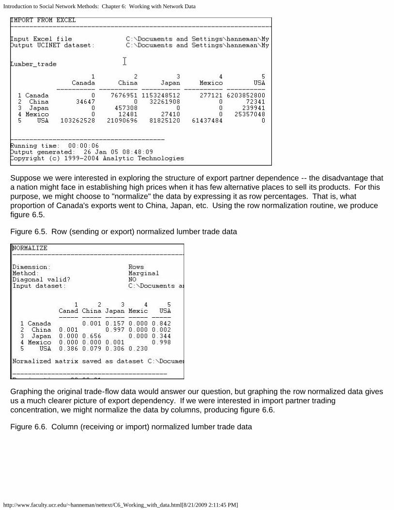
Introduction to Social Network Methods: Chapter 6: Working with Network Data
http://www.faculty.ucr.edu/~hanneman/nettext/C6_Working_with_data.html[8/21/2009 2:11:45 PM]
Suppose we were interested in exploring the structure of export partner dependence -- the disadvantage thata nation might face in establishing high prices when it has few alternative places to sell its products. For thispurpose, we might choose to "normalize" the data by expressing it as row percentages. That is, whatproportion of Canada's exports went to China, Japan, etc. Using the row normalization routine, we producefigure 6.5.
Figure 6.5. Row (sending or export) normalized lumber trade data
Graphing the original trade-flow data would answer our question, but graphing the row normalized data givesus a much clearer picture of export dependency. If we were interested in import partner tradingconcentration, we might normalize the data by columns, producing figure 6.6.
Figure 6.6. Column (receiving or import) normalized lumber trade data

Introduction to Social Network Methods: Chapter 6: Working with Network Data
http://www.faculty.ucr.edu/~hanneman/nettext/C6_Working_with_data.html[8/21/2009 2:11:45 PM]
We see, for example, that all of Canada's imports are from the USA, and that virtually all of the USA'simports are from Canada.
The >Transform>Normalize tool provides a number of ways of re-scaling the data that are frequently used.
Normalization may be applied to either rows or columns (as in our examples, above), or it may be applied tothe entire matrix (for example, rescaling all trade flows as percentages of the total amount of trade flow in thewhole matrix). Normalization may also be applied to both rows and columns, iteratively. For example, if wewanted an "average" number to put in each cell of the trade flow matrix, so that both the rows and thecolumns summed to 100%, we could apply the iterative row and column approach. This is sometimes usedwhen we want to give "equal weight" to each node, and to take into account both outflow (row) and inflow(column) structure.
There are a number of alternative, commonly used, approaches to how to rescale the data. Our examplesuse the "marginal" total (row or column) and set the sum of the entries in each row (or column) to equal 1.0. Alternatively, we might want to express each entry relative to the mean score (e.g. divide each element ofthe row by the average of the elements in a row). Alternatively, one might rescale by dividing by the standarddeviation, or both mean and standard deviation (i.e. express the elements as Z scores). UCINET supportsall of these as built-in functions. In addition, scores can be normalized by Euclidean norm, or by expressingeach element as a percentage of the maximum element in a row.
Rescaling transforms like these can be very, very helpful in highlighting structural features of the data. But,obviously different normalizing approaches highlight very different features. Try thinking through how whatapplying each of the available transformations would tell you for some data that describe a relation that youare interested in. Some of the transformations will be completely useless; some may give you some newideas.
table of contents
File handling tools
Because UCINET data files are stored in a somewhat unusual dual-file format, it is usually most convenientto do basic file-handling tasks within UCINET.The program has basic file handling tools within it. Using thesehas the advantage of automatically dealing with both the .##h and .##d files that make up each UCINETdataset. If you use file handling commands outside UCINET (e.g. using Windows), you need to remember todeal with both files for each data set.

Introduction to Social Network Methods: Chapter 6: Working with Network Data
http://www.faculty.ucr.edu/~hanneman/nettext/C6_Working_with_data.html[8/21/2009 2:11:45 PM]
File utilities:
File>Copy UCINET Dataset
File>Rename UCINET Dataset
File>Delete UCINET Dataset
These commands do exactly what usual operating system commands do, but manage both component fileswith a single command.
Viewing the contents of files:
Data>Browse is a tool for examining parts of a dataset. You select the dataset, and specify which rows,columns, and labels you would like to see. This can be very useful if the dataset you're working with is alarge one, and your interest is in examining only a portion of it.
Data>Display also allows you to modify how you see a data file. You may set field width, numbers ofdecimals to display, whether to show zeros or not; in addition, you can select which rows and/or columns todisplay (the row and column numbers are specified as comma delimited lists, and can use "AND" and "OR"). If the data have been grouped into "blocks," and the block memberships have been stored as UCINETdatasets, these may be used to present the data with members of blocks adjacent to one another.
Data>Describe provides basic information about a file (numbers of rows, columns, matrices). It also showslabels, and allows you import row and column labels from an external text file (just prepare an ASCII text filewith the labels in rows, or comma delimited). You can also use this little utility to add a longer descriptive titleto a UCINET data set. This is often a good idea if you are working with a number of related data sets withsimilar names.
table of contents
Selecting sub-sets of the data
As we work on understanding the structure of a social network, there are occasions when we may wish tofocus our attention on only a portion of the actors. Sometimes it's just a matter of clearing away"underbrush" of nodes that aren't "important." Sometimes it's a matter of selecting sets of actors for separateconsideration.
UCINET has a number of built-in tools that can be useful for creating new data sets from existing data sets,that include only portions of the actors.
Data>Extract is a general-purpose tool that allows you to either "keep" or to "delete" rows, columns, ormatrices for output to a new dataset. You may select the rows, columns, or relations (matrices) to keep bylisting them in external data files, or by choosing the names of the rows, columns or matrices from drop-down lists.
Data>Extract main component retains all the nodes and relations among nodes that are part of the largestcomponent of a graph. In English: the information about the actor and connections among the actors whoare part of the largest set of actors who are all connected is retained. If a graph contains severalcomponents (e.g. if there are some "isolates" or there are sub-groups who have no connection to the largestgroup) only the largest will be retained. Many analyses require that all the nodes be connected. But, not allreal networks actually are. So, you may wish to extract the largest component and analyze it.
Introduction to Social Network Methods: Chapter 6: Working with Network Data
http://www.faculty.ucr.edu/~hanneman/nettext/C6_Working_with_data.html[8/21/2009 2:11:45 PM]
Data>Subgraphs from partitions is a (somewhat more complicated ) tool that let's you divide the cases intogroups (partitions), and output separate data files for each group. The first step (after you've decided whichcases fall in which partition), is to create an external data file that lists partition membership. Suppose Iwanted to put nodes 1, 3, and 5 in one value of a partition (i.e. in one group) and cases 2, 4, and 6 inanother. I'd create a data file that looked like: 1, 2, 1, 2, 1, 2. This says, put the first node in partition one,put the second node in partition two, put the third node in partition one, etc. This filename is supplied to the>Subgraphs from partitions dialog. You may also limit the process by electing to output only certainpartitions (list them in the dialog window), and/or to create new data sets for a partition value only if there aremore than some number (which you specify) of cases.
Many network analysis algorithms generate information on partition membership (and save partitionmembership information as files you can plug in to this utility). You might also want to impose your ownpartitions to identify people in one community, people of a particular gender, etc.
Data>Remove isolates creates a new data set that contains all cases that are not isolated. An "isolate" is acase that has no connections at all to any other actors. Sometimes, when we collect information by doing acensus of all the actors of a given type, or in a given location, some are "isolated." While this is usually aninteresting social fact, we may wish to focus our attention on the community of actors who are connected(though not necessarily forming a single "component").
Data>Remove pendants creates a new data set that contains all cases that are not "pendants." A "pendant"is a case that is connected to the graph by only one tie; cases like these will "dangle" off of more centralcases that are more heavily connected. In looking at large graphs with many actors, we may wish to limit ourattention to nodes that are connected to at least two other actors -- so as to focus attention on the "core" ofthe network. Removing isolates and pendants can help to clear some of the "clutter."
Data>Egonet is a tool that let's us extract particular actors and those in their immediate "neighborhood" asseparate datasets. As we will see later on, the "ego-network" of a single actor, or of some selection of actors(all men, all cases with high between-ness, etc.) is often the focus of investigation more than the structure ofthe whole network.
An "ego-network" is the set of actors who are connected to a focal actor, along with the relations betweenego and the alters, and any relations among the alters. The structure of ego networks (whether they aredense or thin, and whether they contain "structural holes" are often critical variables in understanding andpredicting the behavior of "ego."
The Data>Egonet tool lets you list the "egos" or "focal nodes" you'd like to extract by using an external file listor by selecting their labels from a drop-down list. The dialog asks whether you want to include ego, or onlyto retain information on ego's neighbors; the most common, and default, choice is to include ego as well asego's neighbors.
Data>Unpack is a tool for creating a new data set that contains a sub-set of matrices from a larger data set. For example, if we had stored information on both "liking" and "spouse" relation in a single data set, we canuse this utility to create separate data files for one or both relations. The relations to be "unpacked" areselected from a drop-down box.
Data>Join is a tool that can be used to combine separate sets of data into a new data set. Often we collectattribute information about actors in several different settings (e.g. several classrooms in a school) and storethese as separate files. Or, we may have multiple files that contain information about different attributes ofactors (for example, one file might be things we know from outside sources like age, sex, etc.; another filemight contain information on which partition of a graph each actor falls into). We might want to combine allthe attribute information into a single file. Or, we might have information about different relations among the

Introduction to Social Network Methods: Chapter 6: Working with Network Data
http://www.faculty.ucr.edu/~hanneman/nettext/C6_Working_with_data.html[8/21/2009 2:11:45 PM]
same set of actors, that have been stored as separate data files (as in the "liking" and "spouse" relationsexample).
Using Data>Join>Rows will combine two or more matrices (stored as separate files) into a single matrix thathas rows for all nodes in each of the files. If I had separate files that listed the age of students in each of twoclassrooms, and I wanted to create a single file with all the students, the "rows" approach would be used.
Using Data>Join>Columns will combine two or matrices (stored as separate files) into a single matrix that hasthe same number of rows as each of the input files, but appends the columns. If I had information on ageand sex for actors A, B, and C in one file and information on centrality and degree for actors A, B, and C inanother, I could do a column join to produce a file that listed age, sex, centrality, and degree for actors A, B,and C.
Using Data>Join>Matrices will combine information on multiple relations among the same sets of actors intoa single file. Each input file has the same actors by actors array, but for different relations. The output filecombines the multiple files into a three-dimensional array of actor by actor by relation.
table of contents
Making new kinds of graphs from existing graphs
Turning attributes into relations
At the beginning of this chapter we looked at the "data structures" most commonly used in network analysis. One was the node-by-node square matrix, to record the relations between pairs of actors; and its moregeneral "multi-plex" form to record multiple relations among the same set of actors. The other was therectangular matrix. This "actor by attribute" matrix is most commonly used to record information about thevariable properties of each node.
Network analysis often finds it useful to see actor attributes as actually indicating the presence, absence, orstrength of "relations" among actors. Suppose two persons have the same gender. To the non-networkanalyst, this may represent a statistical regularity that describes the frequencies of scores on a variable. Anetwork analyst, though, might interpret the same data a bit differently. A network analyst might, instead,say "these two persons share the relation of having the same gender."
Both interpretations are, of course, entirely reasonable. One emphasizes the attributes of individuals (hereare two persons, each is a woman); one emphasizes the relation between them (here are two persons whoare related by sharing the same social role).
It's often the case that network researchers, who are pre-disposed to see the world in "relational" terms,want to turn "attribute" data into "relational" data for their analyses.
Data>Attribute is a tool that creates an actor-by-actor relational matrix from the scores on a single attributevector. Suppose that we had an attribute vector stored in a UCINET file (other vectors could also be in thefile, but this algorithm operates on a single vector), that measured whether each of 100 large donors hadgiven funds in support of (+1) or in opposition to (-1) a given ballot proposition. Those who made nocontribution are coded zero.
We might like to create a new matrix that identifies pairs of actors who shared support or shared oppositionto the ballot initiative, or who took opposite positions. That is, for each pair of actors, the matrix element is"1" if the actors jointly supported or jointly opposed the proposition, "-1" if one supported and the otheropposed, and zero otherwise (if either or both made no contribution).
Introduction to Social Network Methods: Chapter 6: Working with Network Data
http://www.faculty.ucr.edu/~hanneman/nettext/C6_Working_with_data.html[8/21/2009 2:11:45 PM]
Using the Data>Attribute tool, we can form a new square (actor-by-actor) matrix from the scores of actors onone attribute in a number of ways. The Exact Matches choice will produce a "1" when two actors haveexactly the same score on the attribute, and zero otherwise. The Difference choice will create a new matrixwhere the elements are the differences between the attribute scores of each pair of actors (alternatively, theAbsolute Difference, or Squared Difference choices will yield positively valued measures of the distancebetween the attribute scores of each pair of actors. The Sum choice yields a score for each pair that is equalto the sum of their attribute scores. In our current example, the Product choice (that is, multiply the score ofactor i times the score of actor j, and enter the result) would yield a score of "1" if two actors shared eithersupport or opposition, "-1" if they took opposed stands on the issue, or "0" if either did not take a position.
The Data>Attribute tool can be very useful for conceptually turning attributes into relations, so that theirassociation with other relations can be studied.
Data>Affiliations extends the idea of turning attributes into relations to the case where we want to consider tomultiple attributes. Probably the most common situations of this type are where the multiple "attributes" wehave measured are "repeated measures" of some sort. Davis, for example, measured the presence of anumber of persons (rows) at a number of parties (attributes or columns). From these data, we might beinterested in the similarity of all pairs of actors (how many times were they co-present at the same event?),or how similar were the parties (how much of the attendance of each pair of parties were the same people?).
The example of donors to political campaigns can be seen in the same way. We might collect information onwhether political donors (rows) had given funds against or for a number different ballot propositions(columns). From this rectangular matrix, we might be interested in forming a square actor by actor matrix(how often do each pair of actors donate to the same campaigns?); we might be interested in forming asquare campaign by campaign matrix (how similar are the campaigns in terms of their constituencies?).
The Data>Affiliations algorithm begins with a rectangular (actor-by-attribute) matrix, and asks you to selectwhether the new matrix is to be formed by rows (i.e. actor-by-actor) or columns (i.e. attribute-by-attribute).
There are different ways in which we could form the entries of the new matrix. UCINET provides twomethods: Cross-Products or Minimums. These approaches produce the same result for binary data, butdifferent results for valued data.
Let's look at the binary case first. Consider two actors "A" and "B" who have made contributions (or not) toeach of 5 political campaigns, as in figure 6.7.
Figure 6.7. Donations of two donors to five political campaigns (binary data)
Campaign 1 Campaign 2 Campaign 3 Campaign 4 Campaign 5"A" 0 0 1 1 1"B" 0 1 1 0 1
The Cross-Products method multiplies each of A's scores by the corresponding score for B, and then sumsacross the columns (if we were creating a campaign-by-campaign matrix, the logic is exactly the same, butwould operate by multiplying columns, and summing across rows). Here, this results in: (0*0) + (0*1) + (1*1)+ (1*0) + (1*1) = 2. That is, actors A and B have two instances where they both supported a campaign.
The Minimums method examines the entries of A and B for campaign 1, and selects the lowest score (zero). It then does this for the other campaigns (resulting in 0, 1, 0, 1) and sums. With binary data, the results willbe the same by either method.

Introduction to Social Network Methods: Chapter 6: Working with Network Data
http://www.faculty.ucr.edu/~hanneman/nettext/C6_Working_with_data.html[8/21/2009 2:11:45 PM]
With valued data, the methods do not produce the same results; they get at rather different ideas.
Suppose that we had measured whether A and B supported (+1), took no position (0), or opposed (-1) eachof the five campaigns. This is the simplest possible "valued" data, but the ideas hold for valued scales withwider ranges, and with all positive values, as well. Now, our data might look like those in figure 6.8.
Figure 6.8. Donations of two donors for or against five political campaigns (valued data)
Campaign 1 Campaign 2 Campaign 3 Campaign 4 Campaign 5"A" -1 0 1 -1 1"B" -1 1 1 0 -1
Both A and B took the same position on two issues (both opposed on one, both supporting another). On twocampaigns (2, 4), one took no stand. On issue number 5, the two actors took opposite positions.
The Cross-products method yields: (-1 * -1) + (0 * 1) + (1 * 1) + (-1 * 0) + (1 * -1). That is: 1 + 0 + 1 + 0 - 1,or 1. The two actors have a "net" agreement of 1 (they took the same position on two issues, but opposedpositions on one issue).
The Minimums method yields: -1 +0 +1 -1-1 or -2. In this example, this is difficult to interpret, but can beseen as the net number of times either member of the pair opposed an issue. The minimums methodproduces results that are easier to interpret when all values are positive. Suppose we re-coded the data tobe: 0 = opposed, 1 = neutral, and 2 = favor. The minimums method would then produce 0 + 1 + 2 + 0 + 0 =3. This might be seen as the extent to which the pair of actors jointly supported the five campaigns.
Turning relations into attributes
Suppose that we had a simple directed relation, represented as a matrix as in figure 6.9.
Figure 6.9. Linegraph example matrix
This is easier to see as a graph, as in figure 6.10.
Figure 6.10. Linegraph example graph

Introduction to Social Network Methods: Chapter 6: Working with Network Data
http://www.faculty.ucr.edu/~hanneman/nettext/C6_Working_with_data.html[8/21/2009 2:11:45 PM]
Now suppose that we are really interested in describing and thinking about the relations, and the relationsamong the relations -- rather than the actors, and the relations among them. That sounds odd, I realize. Letme put it a different way. We can think about the graph in Figure 6.5 as composed of four relations (A to B, Bto C, C to D, and A to C). These relations are connected by having actors in common (e.g. the A to B andthe B to C relations have the actor B in common). That is, we can think about relations as being "adjacent"when they share actors, just as we can think about actors being adjacent when they share relations.
Transform>Incidence is an algorithm that changes the way we look at a directed graph from "actorsconnected by relations" to "relations connected by actors." This is sometimes just a semantic trick. But,sometimes it's more than that -- our theory of the social structure may actually be one about which relationsare connected, not which actors are connected. If we apply the Transform>Incidence algorithm to the data infigures 6.4 and 6.5, we get the result in figure 6.11.
Figure 6.11. Incidence matrix of graph 6.10
Each row is an actor. Each column is now a relation (the relations are numbered 1 through 4). A positiveentry indicates that an actor is the source of a a directed relation. For example, actor A is the origin of therelation "1" that connects A to B, and is a source of the relation "2" that connects actor A to actor D. Anegative entry indicates that an actor is the "sink" or recipient of a directed relation. For example, actor C isthe recipient in relation "3" (which connects actor B to actor C), and the source of relation "4" (whichconnects actor C to actor D.
The "incidence" matrix here then shows how actors are connected to relationships. By examining the rows,we can characterize how much, and in what ways actors are embedded in relations. One actor may havefew entries -- a near isolate; another may have many negative and few positive entries -- a "taker" ratherthan a "giver." By examining the columns, we get a description of which actors are connected, in which way,by each of the relations in the graph.
Focusing on the relations, instead of the actors
Turning an actor-by-actor adjacency matrix into an actor-by-relation incidence graph takes us part of the waytoward focusing on relations rather than actors. We can go further.

Introduction to Social Network Methods: Chapter 6: Working with Network Data
http://www.faculty.ucr.edu/~hanneman/nettext/C6_Working_with_data.html[8/21/2009 2:11:45 PM]
Transform> Linegraph converts an actor-by-actor matrix (like figure 6.4) into a full relation-by-relation matrix. Figure 6.12 shows the results of applying it to the example data.
Figure 6.12. Linegraph matrix
We again have a square matrix. This time, though, it describes which relations in the graph are "adjacent to"which other relations. Two relations are adjacent if they share an actor. For example, relation "1" (the tiebetween actors 1 and 2, or A and B) is adjacent to the relation "3" (the tie between actors 2 and 3, or B andC). Note that the "adjacency" here is directional -- relation 1 is a source of relation 3. We could also applythis approach to symmetric or simple graphs to describe which relations are simply adjacent in a un-directedway.
A quick glance at the linegraph matrix is suggestive. It is very sparse in this example -- most of the relationsare not sources of other relations. The maximum degree of each entry is 1 -- no relation is the source ofmultiple relations. While there may be a key or central actor (A), it's not so clear that there is a single centralrelation.
To be entirely honest, most social network analysts do (much of the time) think about actors connected toactors by relations, rather than relations connecting actors, or relations connecting relations. But changingour point of view to put the relations first, and the actors second is, in many ways, a more distinctively"sociological" way of looking at networks. Transforming actor-by-actor data into relation-by-relation data canyield some interesting insights about social structures.
table of contents
Conclusion
In this chapter we've covered a number of rather diverse but related topics. We've described some of thebasic "nuts and bolts" tools for entering and transforming network data. The "bigger picture" is to think aboutnetwork data (and any other, for that matter) as having "structure." Once you begin to see data in this way,you can begin to better imagine the creative possibilities: for example, treating actor-by-attribute data asactor-by-actor, or treating it as attribute-by-attribute. Different research problems may call for quite differentways of looking at, and transforming, the same data structures. We've hardly covered every possibility here,but we have looked at some of the most frequently used tricks.
top of this pagetable of contents of the book

Introduction to Social Network Methods: Chapter 7: Basic Properties of Networks and Actors
http://www.faculty.ucr.edu/~hanneman/nettext/C7_Connection.html[8/21/2009 2:12:06 PM]
Introduction to social network methods
7. Connection and distance
This page is part of an on-line text by Robert A. Hanneman (Department of Sociology, University of California, Riverside) and MarkRiddle (Department of Sociology, University of Northern Colorado). Feel free to use and distribute this textbook, with citation. Yourcomments and suggestions are very welcome. Send me e-mail.
Contents of chapter 7: Connection and distance
Networks and actorsAn example: Knoke's information exchange
ConnectionBasic demographicsDensityReachabilityConnectivity
DistanceWalks etc.Geodesic distance, eccentricity, and diameterFlow
SummaryStudy Questions
Networks and actors
The social network perspective emphasizes multiple levels of analysis. Differences among actors are tracedto the constraints and opportunities that arise from how they are embedded in networks; the structure andbehavior of networks grounded in, and enacted by local interactions among actors. As we examine some ofthe basic concepts and definitions of network analysis in this and the next several chapters, this duality ofindividual and structure will be highlighted again and again.
In this chapter we will examine some of the most obvious and least complex ideas of formal network analysismethods. Despite the simplicity of the ideas and definitions, there are good theoretical reasons (and someempirical evidence) to believe that these basic properties of social networks have very importantconsequences. For both individuals and for structures, one main question is connections. Typically, someactors have lots of of connections, others have fewer. Some networks are well-connected or "cohesive,"others are not. The extent to which individuals are connected to others, and the extent to which the networkas a whole is integrated are two sides of the same coin.
Differences among individuals in how connected they are can be extremely consequential for understandingtheir attributes and behavior. More connections often mean that individuals are exposed to more, and morediverse, information. Highly connected individuals may be more influential, and may be more influenced byothers. Differences among whole populations in how connected they are can be quite consequential as well.Disease and rumors spread more quickly where there are high rates of connection. But, so to does usefulinformation. More connected populations may be better able to mobilize their resources, and may be betterable to bring multiple and diverse perspectives to bear to solve problems. In between the individual and thewhole population, there is another level of analysis -- that of "composition." Some populations may becomposed of individuals who are all pretty much alike in the extent to which they are connected. Other
Introduction to Social Network Methods: Chapter 7: Basic Properties of Networks and Actors
http://www.faculty.ucr.edu/~hanneman/nettext/C7_Connection.html[8/21/2009 2:12:06 PM]
populations may display sharp differences, with a small elite of central and highly connected persons, andlarger masses of persons with fewer connections. Differences in connections can tell us a good bit about thestratification order of social groups. A great deal of recent work by Duncan Watts, Doug White and manyothers outside of the social sciences is focusing on the consequences of variation in the degree ofconnection of actors.
Because most individuals are not usually connected directly to most other individuals in a population, it canbe quite important to go beyond simply examining the immediate connections of actors, and the overalldensity of direct connections in populations. The second major (but closely related) set of approaches thatwe will examine in this chapter have to do with the idea of the distance between actors (or, conversely howclose they are to one another). Some actors may be able to reach most other members of the populationwith little effort: they tell their friends, who tell their friends, and "everyone" knows. Other actors may havedifficulty being heard. They may tell people, but the people they tell are not well connected, and the messagedoesn't go far. Thinking about it the other way around, if all of my friends have one another as friends, mynetwork is fairly limited -- even though I may have quite a few friends. But, if my friends have many non-overlapping connections, the range of my connection is expanded. If individuals differ in their closeness toother actors, then the possibility of stratification along this dimension arises. Indeed, one major differenceamong "social classes" is not so much in the number of connections that actors have, but in whether theseconnections overlap and "constrain" or extent outward and provide "opportunity." Populations as a whole,then, can also differ in how close actors are to other actors, on the average. Such differences may help us tounderstand diffusion, homogeneity, solidarity, and other differences in macro properties of social groups.
Social network methods have a vocabulary for describing connectedness and distance that might, at first,seem rather formal and abstract. This is not surprising, as many of the ideas are taken directly from themathematical theory of graphs. But it is worth the effort to deal with the jargon. The precision and rigor of thedefinitions allow us to communicate more clearly about important properties of social structures -- and oftenlead to insights that we would not have had if we used less formal approaches.
table of contents
An example: Knoke's information exchange
The basic properties of networks are easier to learn and understand by example. Studying an example alsoshows sociologically meaningful applications of the formalisms. In this chapter, we will look at a singledirected binary network that describes the flow of information among 10 formal organizations concerned withsocial welfare issues in one mid-western U.S. city (Knoke and Burke). Of course, network data come inmany forms (undirected, multiple ties, valued ties, etc.) and one example can't capture all of the possibilities.Still, it can be rather surprising how much information can be "squeezed out" of a single binary matrix byusing basic graph concepts.
For small networks, it is often useful to examine graphs. Figure 7.1 shows the di-graph (directed graph) forthe Knoke information exchange data:
Figure 7.1 Knoke information exchange directed graph

Introduction to Social Network Methods: Chapter 7: Basic Properties of Networks and Actors
http://www.faculty.ucr.edu/~hanneman/nettext/C7_Connection.html[8/21/2009 2:12:06 PM]
Your trained eye should immediately perceive a number of things in looking at the graph. There are a limitednumber of actors here (ten, actually), and all of them are "connected." But, clearly not every possibleconnection is present, and there are "structural holes" (or at least "thin spots" in the fabric). There appear tobe some differences among the actors in how connected they are (compare actor number 7, a newspaper, toactor number 6, a welfare rights advocacy organization). If you look closely, you can see that some actor'sconnections are likely to be reciprocated (that is, if A shares information with B, B also shares informationwith A); some other actors (e.g. 6 and 10, are more likely to be senders than receivers of information). As aresult of the variation in how connected individuals are, and whether the ties are reciprocated, some actorsmay be at quite some "distance" from other actors. There appear to be groups of actors who differ in thisregard (2, 5, and 7 seem to be in the center of the action, 6, 9, and 10 seem to be more peripheral).
A careful look at the graph can be very useful in getting an intuitive grasp of the important features of a socialnetwork. With larger populations or more connections, however, graphs may not be much help. Looking at agraph can give a good intuitive sense of what is going on, but our descriptions of what we see are ratherimprecise (the previous paragraph is an example of this). To get more precise, and to use computers toapply algorithms to calculate mathematical measures of graph properties, it is necessary to work with theadjacency matrix instead of the graph. The Knoke data graphed above are shown as an asymmetricadjacency matrix in figure 7.2.
Figure 7.2 Knoke information exchange adjacency matrix

Introduction to Social Network Methods: Chapter 7: Basic Properties of Networks and Actors
http://www.faculty.ucr.edu/~hanneman/nettext/C7_Connection.html[8/21/2009 2:12:06 PM]
Using Data>Display, we can look at the network in matrix form. There are ten rows and columns, the dataare binary, and the matrix is asymmetric. As we mentioned in the chapter on using matrices to representnetworks, the row is treated as the source of information and the column as the receiver. By doing some verysimple operations on this matrix it is possible to develop systematic and useful index numbers, or measures,of some of the network properties that our eye discerns in the graph.
table of contents
Connection
Since networks are defined by their actors and the connections among them, it is useful to begin ourdescription of networks by examining these very simple properties. Focusing first on the network as a whole,one might be interested in the number of actors, the number of connections that are possible, and thenumber of connections that are actually present. Differences in the size of networks, and how connected theactors are tell us two things about human populations that are critical. Small groups differ from large groupsin many important ways -- indeed, population size is one of the most critical variables in all sociologicalanalyses. Differences in how connected the actors in a population are may be a key indicator of the"cohesion," "solidarity," "moral density," and "complexity" of the social organization of a population.
Individuals, as well as whole networks, differ in these basic demographic features. Individual actors mayhave many or few ties. Individuals may be "sources" of ties, "sinks" (actors that receive ties, but don't sendthem), or both. These kinds of very basic differences among actors immediate connections may be critical inexplaining how they view the world, and how the world views them. The number and kinds of ties that actorshave are a basis for similarity or dissimilarity to other actors -- and hence to possible differentiation andstratification. The number and kinds of ties that actors have are keys to determining how much theirembeddedness in the network constrains their behavior, and the range of opportunities, influence, and powerthat they have.
table of contents
Basic demographics
Network size. The size of a network is often very important. Imagine a group of 12 students in a seminar. Itwould not be difficult for each of the students to know each of the others fairly well, and build up exchangerelationships (e.g. sharing reading notes). Now imagine a large lecture class of 300 students. It would beextremely difficult for any student to know all of the others, and it would be virtually impossible for there to bea single network for exchanging reading notes. Size is critical for the structure of social relations because ofthe limited resources and capacities that each actor has for building and maintaining ties. Our examplenetwork has ten actors. Usually the size of a network is indexed simply by counting the number of nodes.

Introduction to Social Network Methods: Chapter 7: Basic Properties of Networks and Actors
http://www.faculty.ucr.edu/~hanneman/nettext/C7_Connection.html[8/21/2009 2:12:06 PM]
In any network there are (k * k-1) unique ordered pairs of actors (that is AB is different from BA, and leavingaside self-ties), where k is the number of actors. You may wish to verify this for yourself with some smallnetworks. So, in our network of 10 actors, with directed data, there are 90 logically possible relationships. Ifwe had undirected, or symmetric ties, the number would be 45, since the relationship AB would be the sameas BA. The number of logically possible relationships then grows exponentially as the number of actorsincreases linearly. It follows from this that the range of logically possible social structures increases (or, byone definition, "complexity" increases) exponentially with size.
Actor degree. The number of actors places an upper limit on the number of connections that each individualcan have (k-1). For networks of any size, though, few -- if any -- actors approach this limit. It can be quiteuseful to examine the distribution of actor degree. The distribution of how connected individual actors arecan tell us a good bit about the social structure.
Since the data in our example are asymmetric (that is directed ties), we can distinguish between ties beingsent and ties being received. Looking at the density for each row and for each column can tell us a good bitabout the way in which actors are embedded in the overall density.
Tools>Univariate Stats provides quick summaries of the distribution of actor's ties.
Let's first examine these statistics for the rows, or out-degree of actors.
Figure 7.3. Dialog for Tools>Univariate Stats
Produces this result:
Figure 7.4. Out-degree statistics for Knoke information exchange
Statistics on the rows tell us about the role that each actor plays as a "source" of ties (in a directed graph).The sum of the connections from the actor to others (e.g. actor #1 sends information to four others) is calledthe out-degree of the point (for symmetric data, of course, each node simply has degree, as we cannotdistinguish in-degree from out-degree). The degree of points is important because it tells us how many
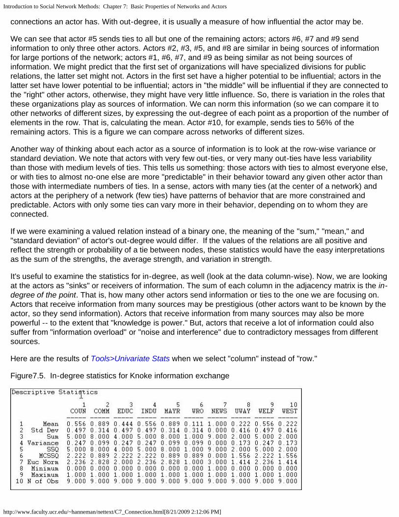
Introduction to Social Network Methods: Chapter 7: Basic Properties of Networks and Actors
http://www.faculty.ucr.edu/~hanneman/nettext/C7_Connection.html[8/21/2009 2:12:06 PM]
connections an actor has. With out-degree, it is usually a measure of how influential the actor may be.
We can see that actor #5 sends ties to all but one of the remaining actors; actors #6, #7 and #9 sendinformation to only three other actors. Actors #2, #3, #5, and #8 are similar in being sources of informationfor large portions of the network; actors #1, #6, #7, and #9 as being similar as not being sources ofinformation. We might predict that the first set of organizations will have specialized divisions for publicrelations, the latter set might not. Actors in the first set have a higher potential to be influential; actors in thelatter set have lower potential to be influential; actors in "the middle" will be influential if they are connected tothe "right" other actors, otherwise, they might have very little influence. So, there is variation in the roles thatthese organizations play as sources of information. We can norm this information (so we can compare it toother networks of different sizes, by expressing the out-degree of each point as a proportion of the number ofelements in the row. That is, calculating the mean. Actor #10, for example, sends ties to 56% of theremaining actors. This is a figure we can compare across networks of different sizes.
Another way of thinking about each actor as a source of information is to look at the row-wise variance orstandard deviation. We note that actors with very few out-ties, or very many out-ties have less variabilitythan those with medium levels of ties. This tells us something: those actors with ties to almost everyone else,or with ties to almost no-one else are more "predictable" in their behavior toward any given other actor thanthose with intermediate numbers of ties. In a sense, actors with many ties (at the center of a network) andactors at the periphery of a network (few ties) have patterns of behavior that are more constrained andpredictable. Actors with only some ties can vary more in their behavior, depending on to whom they areconnected.
If we were examining a valued relation instead of a binary one, the meaning of the "sum," "mean," and"standard deviation" of actor's out-degree would differ. If the values of the relations are all positive andreflect the strength or probability of a tie between nodes, these statistics would have the easy interpretationsas the sum of the strengths, the average strength, and variation in strength.
It's useful to examine the statistics for in-degree, as well (look at the data column-wise). Now, we are lookingat the actors as "sinks" or receivers of information. The sum of each column in the adjacency matrix is the in-degree of the point. That is, how many other actors send information or ties to the one we are focusing on.Actors that receive information from many sources may be prestigious (other actors want to be known by theactor, so they send information). Actors that receive information from many sources may also be morepowerful -- to the extent that "knowledge is power." But, actors that receive a lot of information could alsosuffer from "information overload" or "noise and interference" due to contradictory messages from differentsources.
Here are the results of Tools>Univariate Stats when we select "column" instead of "row."
Figure7.5. In-degree statistics for Knoke information exchange

Introduction to Social Network Methods: Chapter 7: Basic Properties of Networks and Actors
http://www.faculty.ucr.edu/~hanneman/nettext/C7_Connection.html[8/21/2009 2:12:06 PM]
Looking at the means, we see that there is a lot of variation in information receiving -- more than forinformation sending. We see that actors #2, #5, and #7 are very high. #2 and #5 are also high in sendinginformation -- so perhaps they act as "communicators" and "facilitators" in the system. Actor #7 receives a lotof information, but does not send a lot. Actor #7, as it turns out is an "information sink" -- it collects facts, butit does not create them (at least we hope so, since actor #7 is a newspaper). Actors #6, #8, and #10 appearto be "out of the loop" -- that is, they do not receive information from many sources directly. Actor #6 alsodoes not send much information -- so #6 appears to be something of an "isolate." Numbers #8 and #10 sendrelatively more information than they receive. One might suggest that they are "outsiders" who areattempting to be influential, but may be "clueless."
We can learn a great deal about a network overall, and about the structural constraints on individual actors,and even start forming some hypotheses about social roles and behavioral tendencies, just by looking at thesimple adjacencies and calculating a few very basic statistics. Before discussing the slightly more complexidea of distance, there are a couple other aspects of "connectedness" that are sometimes of interest.
table of contents
Density
The density of a binary network is simply the proportion of all possible ties that are actually present. For avalued network, density is defined as the sum of the ties divided by the number of possible ties (i.e. the ratioof all tie strength that is actually present to the number of possible ties). The density of a network may giveus insights into such phenomena as the speed at which information diffuses among the nodes, and theextent to which actors have high levels of social capital and/or social constraint.
Network>Cohesion>Density is a quite powerful tool for calculating densities. its dialog is shown in figure 7.6.
Figure 7.6 Dialog for Network>Cohesion>Density
To obtain densities for a matrix (as we are doing in this example), we simply need a dataset. Usually self-ties are ignored in computing density (but there are circumstances where you might want to include them). The Network>Cohesion>Density algorithm also can be used to calculate the densities within partitions orblocks by specifying the file name of an attribute data set that contains the node name and partition number. That is, the density tool can be used to calculate within and between block densities for data that aregrouped. One might, for example, partition the Knoke data into "public" and "private" organizations, andexamine the density of information exchange within and between types.
For our current purposes, we won't block or partition the data. Here's the result of the dialog above.

Introduction to Social Network Methods: Chapter 7: Basic Properties of Networks and Actors
http://www.faculty.ucr.edu/~hanneman/nettext/C7_Connection.html[8/21/2009 2:12:06 PM]
Figure 7.7 Density of Knoke information network
Since the Knoke data set contains two matrices, separate reports for each relation (KNOKI and KNOKM) areproduced.
The density of the information exchange relation matrix is .5444. That is 54% of all the possible ties arepresent. The standard deviation of the entries in the matrix is also given. For binary data, the standarddeviation is largely irrelevant -- as the standard deviation of a binary variable is a function of its mean.
Reachability
An actor is "reachable" by another if there exists any set of connections by which we can trace from thesource to the target actor, regardless of how many others fall between them. If the data are asymmetric ordirected, it is possible that actor A can reach actor B, but that actor B cannot reach actor A. With symmetricor undirected data, of course, each pair of actors either are or are not reachable to one another. If someactors in a network cannot reach others, there is the potential of a division of the network. Or, it may indicatethat the population we are studying is really composed of more than one sub-populations.
In the Knoke information exchange data set, it turns out that all actors are reachable by all others. This issomething that you can verify by eye. See if you can find any pair of actors in the diagram such that youcannot trace from the first to the second along arrows all headed in the same direction (don't waste a lot oftime on this, there is no such pair!). For the Knoke "M" relation, it turns out that not all actors can "reach" allother actors. Here's the output of Network>Cohesion>Reachability from UCINET.
Figure 7.8 Reachability of Knoke "I" and "M" relations
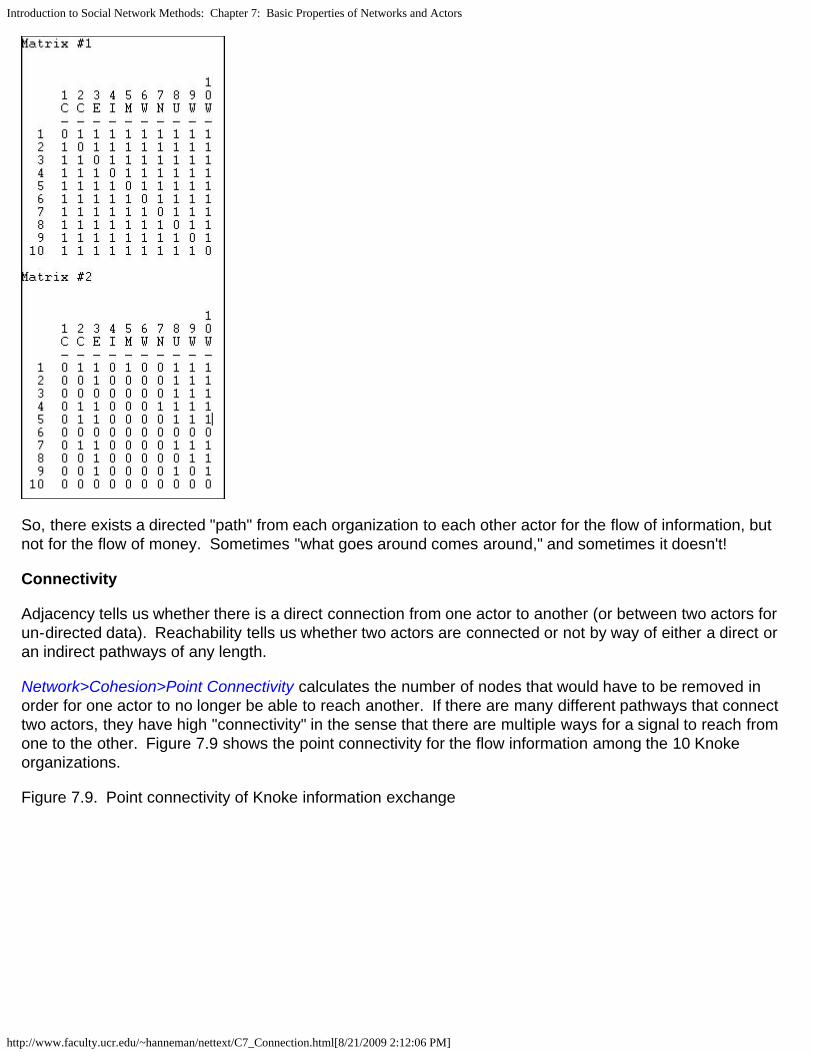
Introduction to Social Network Methods: Chapter 7: Basic Properties of Networks and Actors
http://www.faculty.ucr.edu/~hanneman/nettext/C7_Connection.html[8/21/2009 2:12:06 PM]
So, there exists a directed "path" from each organization to each other actor for the flow of information, butnot for the flow of money. Sometimes "what goes around comes around," and sometimes it doesn't!
Connectivity
Adjacency tells us whether there is a direct connection from one actor to another (or between two actors forun-directed data). Reachability tells us whether two actors are connected or not by way of either a direct oran indirect pathways of any length.
Network>Cohesion>Point Connectivity calculates the number of nodes that would have to be removed inorder for one actor to no longer be able to reach another. If there are many different pathways that connecttwo actors, they have high "connectivity" in the sense that there are multiple ways for a signal to reach fromone to the other. Figure 7.9 shows the point connectivity for the flow information among the 10 Knokeorganizations.
Figure 7.9. Point connectivity of Knoke information exchange

Introduction to Social Network Methods: Chapter 7: Basic Properties of Networks and Actors
http://www.faculty.ucr.edu/~hanneman/nettext/C7_Connection.html[8/21/2009 2:12:06 PM]
The result again demonstrates the tenuousness of organization 6's connection as both a source (row) orreceiver (column) of information. To get its message to most other actors, organization 6 has alternative;should a single organization refuse to pass along information, organization 6 would receive none at all! Pointconnectivity can be a useful measure to get at notions of dependency and vulnerability.
table of contents
Distance
The properties of the network that we have examined so far primarily deal with adjacencies -- the directconnections from one actor to the next. But the way that people are embedded in networks is more complexthan this. Two persons, call them A and B, might each have five friends. But suppose that none of person A'sfriends have any friends except A. Person B's five friends, in contrast, each have five friends. The informationavailable to B, and B's potential for influence is far greater than A's. That is, sometimes being a "friend of afriend" may be quite consequential.
To capture this aspect of how individuals are embedded in networks, one main approach is to examine thedistance that an actor is from others. If two actors are adjacent, the distance between them is one (that is, ittakes one step for a signal to go from the source to the receiver). If A tells B, and B tells C (and A does nottell C), then actors A and C are at a distance of two. How many actors are at various distances from eachactor can be important for understanding the differences among actors in the constraints and opportunitiesthey have as a result of their position. Sometimes we are also interested in how many ways there are toconnect between two actors, at a given distance. That is, can actor A reach actor B in more than one way?Sometimes multiple connections may indicate a stronger connection between two actors than a singleconnection.
The distances among actors in a network may be an important macro-characteristic of the network as awhole. Where distances are great, it may take a long time for information to diffuse across a population. Itmay also be that some actors are quite unaware of, and influenced by others -- even if they are technicallyreachable, the costs may be too high to conduct exchanges. The variability across the actors in thedistances that they have from other actors may be a basis for differentiation and even stratification. Thoseactors who are closer to more others may be able to exert more power than those who are more distant. Wewill have a good deal more to say about this aspect of variability in actor distances in the next chapter.
For the moment, we need to learn a bit of jargon that is used to describe the distances between actors:walks, paths, semi-paths, etc. Using these basic definitions, we can then develop some more powerful waysof describing various aspects of the distances among actors in a network.
table of contents
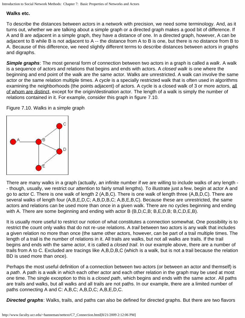
Introduction to Social Network Methods: Chapter 7: Basic Properties of Networks and Actors
http://www.faculty.ucr.edu/~hanneman/nettext/C7_Connection.html[8/21/2009 2:12:06 PM]
Walks etc.
To describe the distances between actors in a network with precision, we need some terminology. And, as itturns out, whether we are talking about a simple graph or a directed graph makes a good bit of difference. IfA and B are adjacent in a simple graph, they have a distance of one. In a directed graph, however, A can beadjacent to B while B is not adjacent to A -- the distance from A to B is one, but there is no distance from B toA. Because of this difference, we need slightly different terms to describe distances between actors in graphsand digraphs.
Simple graphs: The most general form of connection between two actors in a graph is called a walk. A walkis a sequence of actors and relations that begins and ends with actors. A closed walk is one where thebeginning and end point of the walk are the same actor. Walks are unrestricted. A walk can involve the sameactor or the same relation multiple times. A cycle is a specially restricted walk that is often used in algorithmsexamining the neighborhoods (the points adjacent) of actors. A cycle is a closed walk of 3 or more actors, allof whom are distinct, except for the origin/destination actor. The length of a walk is simply the number ofrelations contained in it. For example, consider this graph in figure 7.10.
Figure 7.10. Walks in a simple graph
There are many walks in a graph (actually, an infinite number if we are willing to include walks of any length -- though, usually, we restrict our attention to fairly small lengths). To illustrate just a few, begin at actor A andgo to actor C. There is one walk of length 2 (A,B,C). There is one walk of length three (A,B,D,C). There areseveral walks of length four (A,B,E,D,C; A,B,D,B,C; A,B,E,B,C). Because these are unrestricted, the sameactors and relations can be used more than once in a given walk. There are no cycles beginning and endingwith A. There are some beginning and ending with actor B (B,D,C,B; B,E,D,B; B,C,D,E,B).
It is usually more useful to restrict our notion of what constitutes a connection somewhat. One possibility is torestrict the count only walks that do not re-use relations. A trail between two actors is any walk that includesa given relation no more than once (the same other actors, however, can be part of a trail multiple times. Thelength of a trail is the number of relations in it. All trails are walks, but not all walks are trails. If the trailbegins and ends with the same actor, it is called a closed trail. In our example above, there are a number oftrails from A to C. Excluded are tracings like A,B,D,B,C (which is a walk, but is not a trail because the relationBD is used more than once).
Perhaps the most useful definition of a connection between two actors (or between an actor and themself) isa path. A path is a walk in which each other actor and each other relation in the graph may be used at mostone time. The single exception to this is a closed path, which begins and ends with the same actor. All pathsare trails and walks, but all walks and all trails are not paths. In our example, there are a limited number ofpaths connecting A and C: A,B,C; A,B,D,C; A,B,E,D,C.
Directed graphs: Walks, trails, and paths can also be defined for directed graphs. But there are two flavors

Introduction to Social Network Methods: Chapter 7: Basic Properties of Networks and Actors
http://www.faculty.ucr.edu/~hanneman/nettext/C7_Connection.html[8/21/2009 2:12:06 PM]
of each, depending on whether we want to take direction into account or not . Semi-walks, semi-trails, andsemi-paths are the same as for undirected data. In defining these distances, the directionality of connectionsis simply ignored (that is, arcs - or directed ties are treated as though they were edges - undirected ties). Asalways, the length of these distances is the number of relations in the walk, trail, or path.
If we do want to pay attention to the directionality of the connections we can define walks, trails, and paths inthe same way as before, but with the restriction that we may not "change direction" as we move acrossrelations from actor to actor. Consider the directed graph in figure 7.11
Figure 7.11. Walks in a directed graph
In this directed graph, there are a number of walks from A to C. However, there are no walks from C (oranywhere else) to A. Some of these walks from A to C are also trails (e.g. A,B,E,D,B,C). There are, however,only three paths from A to C. One path is length 2 (A,B,C); one is length three (A,B,D,C); one is length four(A,B,E,D,C).
The various kinds of connections (walks, trails, paths) provide us with a number of different ways of thinkingabout the distances between actors. The main reason that social network analysts are concerned with thesedistances is that they provide a way of thinking about the strength of ties or relations. Actors that areconnected at short lengths or distances may have stronger connections; actors that are connected manytimes (for example, having many, rather than a single path) may have stronger ties. Their connection mayalso be less subject to disruption, and hence more stable and reliable.
The numbers of walks of a given length between all pairs of actors can be found by raising the matrix to thatpower. A convenient method for accomplishing this is to use Tools>Matrix Algebra, and to specify anexpression like out=prod(X1,X1). This produces the square of the matrix X1, and stores it as the data set"out." A more detailed discussion of this idea can be found in the earlier chapter on representing networksas matrices. This matrix could then be added to X1 to show the number of walks between any two actors oflength two or less.
Let's look briefly at the distances between pairs of actors in the Knoke data on directed information flows. Counts of the numbers of paths of various lengths are shown in figure 7.12.
Figure 7.12. Numbers of walks in Knoke information network
# of walks of length 1 1 1 2 3 4 5 6 7 8 9 0 - - - - - - - - - - 1 0 1 0 0 1 0 1 0 1 0 2 1 0 1 1 1 0 1 1 1 0 3 0 1 0 1 1 1 1 0 0 1

Introduction to Social Network Methods: Chapter 7: Basic Properties of Networks and Actors
http://www.faculty.ucr.edu/~hanneman/nettext/C7_Connection.html[8/21/2009 2:12:06 PM]
4 1 1 0 0 1 0 1 0 0 0 5 1 1 1 1 0 0 1 1 1 1 6 0 0 1 0 0 0 1 0 1 0 7 0 1 0 1 1 0 0 0 0 0 8 1 1 0 1 1 0 1 0 1 0 9 0 1 0 0 1 0 1 0 0 0 10 1 1 1 0 1 0 1 0 0 0
# of walks of length 2 1 1 2 3 4 5 6 7 8 9 0 - - - - - - - - - - 1 2 3 2 3 3 0 3 2 2 1 2 3 7 1 4 6 1 6 1 3 2 3 4 4 4 3 4 0 5 2 3 1 4 2 3 2 3 3 0 3 2 3 1 5 4 7 2 4 8 1 7 1 3 1 6 0 3 0 2 3 1 2 0 0 1 7 3 2 2 2 2 0 3 2 2 1 8 3 5 2 3 5 0 5 2 3 1 9 2 2 2 3 2 0 2 2 2 1 10 2 4 2 4 4 1 4 2 3 2
# of walks of length 3 1 2 3 4 5 6 7 8 9 10 -- -- -- -- -- -- -- -- -- -- 1 12 18 7 13 18 2 18 6 10 5 2 20 26 16 21 27 1 28 13 18 7 3 14 26 9 19 26 4 25 8 14 8 4 12 19 7 13 19 2 19 6 10 5 5 21 30 17 25 29 2 31 15 21 10 6 9 8 8 8 8 0 10 6 7 3 7 9 17 5 11 17 2 16 4 9 4 8 16 24 11 19 24 2 24 10 15 7 9 10 16 5 10 16 2 16 4 8 4 10 16 23 11 16 23 2 24 8 13 6
Total number of walks (lengths 1, 2, 3) 1 2 3 4 5 6 7 8 9 10 -- -- -- -- -- -- -- -- -- -- 1 14 21 9 16 21 2 21 8 12 6 2 23 33 17 25 33 2 34 14 21 9 3 18 30 13 22 30 4 30 10 17 9 4 14 22 9 16 22 2 22 8 13 6 5 25 37 19 29 37 3 38 16 24 11 6 9 11 8 10 11 1 12 6 7 4 7 12 19 7 13 19 2 19 6 11 5 8 19 29 13 22 29 2 29 12 18 8 9 12 18 7 13 18 2 18 6 10 5 10 18 27 13 20 27 3 28 10 16 8
The inventory of the total connections among actors is primarily useful for getting a sense of how "close"each pair is, and for getting a sense of how closely coupled the entire system is. Here, we can see that usingonly connections of two steps (e.g. "A friend of a friend"), there is a great deal of connection in the graphoverall; we also see that there are sharp differences among actors in their degree of connectedness, andwho they are connected to. These differences can be used to understand how information moves in thenetwork, which actors are likely to be influential on one another, and a number of other important properties.
table of contents
Geodesic distance, eccentricity, and diameter
One particular definition of the distance between actors in a network is used by most algorithms to definemore complex properties of individual's positions and the structure of the network as a whole. This quantity isthe geodesic distance. For both directed and undirected data, the geodesic distance is the number ofrelations in the shortest possible walk from one actor to another (or, from an actor to themselves, if we care,which we usually do not).
The geodesic distance is widely used in network analysis. There may be many connections between two

Introduction to Social Network Methods: Chapter 7: Basic Properties of Networks and Actors
http://www.faculty.ucr.edu/~hanneman/nettext/C7_Connection.html[8/21/2009 2:12:06 PM]
actors in a network. If we consider how the relation between two actors may provide each with opportunityand constraint, it may well be the case that not all of these ties matter. For example, suppose that I am tryingto send a message to Sue. Since I know her e-mail address, I can send it directly (a path of length 1). I alsoknow Donna, and I know that Donna has Sue's email address. I could send my message for Sue to Donna,and ask her to forward it. This would be a path of length two. Confronted with this choice, I am likely tochoose the geodesic path (i.e. directly to Sue) because it is less trouble and faster, and because it does notdepend on Donna. That is, the geodesic path (or paths, as there can be more than one) is often the "optimal"or most "efficient" connection between two actors. Many algorithms in network analysis assume that actorswill use the geodesic path when alternatives are available.
Using UCINET, we can easily locate the lengths of the geodesic paths in our directed data on informationexchanges. Here is the dialog box for Network>Cohesion>Distance.
Figure 7.13. Network>Cohesion>Distance dialog
The Knoke information exchange data are binary (organization A sends information to organization B, or itdoesn't). That is, the pattern is summarized by an adjacency matrix. For binary data, the geodesic distancebetween two actors is the count of the number of links in the shortest path between them.
It is also possible to define the distance between two actors where the links are valued. That is, where wehave a measure of the strength of ties, the opportunity costs of ties, or the probability of a tie. Network>Cohesion>Distance can calculate distance (and nearness) for valued data, as well (select theappropriate "type of data").
Where we have measures of the strengths of ties (e.g. the dollar volume of trade between two nations), the"distance" between two actors is defined as the strength of the weakest path between them. If A sends 6units to B, and B sends 4 units to C, the "strength" of the path from A to C (assuming A to B to C is theshortest path) is 4.
Where we have a measure of the cost of making a connection (as in an "opportunity cost" or "transactioncost" analysis), the "distance" between two actors is defined as the sum of the costs along the shortestpathway.
Where we have a measure of the probability that a link will be used, the "distance" between two actors isdefined as the product along the pathway -- as in path analysis in statistics.
The Nearness Transformation and Attenuation Factor parts of the dialog allow the rescaling of distances intonear-nesses. For many analyses, we may be interesting in thinking about the connections among actors interms of how close or similar they are, rather than how distant. There are a number of ways that this may bedone.

Introduction to Social Network Methods: Chapter 7: Basic Properties of Networks and Actors
http://www.faculty.ucr.edu/~hanneman/nettext/C7_Connection.html[8/21/2009 2:12:06 PM]
The multiplicative nearness transformation divides the distance by the largest possible distance between twoactors. For example, if we had 7 nodes, the maximum possible distance for adjacency data would be 6. Thismethod gives a measure of the distance as a percentage of the theoretical maximum for a given graph.
The additive nearness transformation subtracts the actual distance between two actors from the number ofnodes. It is similar to the multiplicative scaling, but yields a value as the nearness measure, rather than aproportion.
The linear nearness transformation rescales distance by reversing the scale (i.e. the closest becomes themost distant, the most distant becomes the nearest) and re-scoring to make the scale range from zero(closest pair of nodes) to one (most distant pair of nodes).
The exponential decay method turns distance into nearness by weighting the links in the pathway withdecreasing values as they fall farther away from ego. With an attenuation factor of .5, for example, a pathfrom A to B to C would result in a distance of 1.5.
The frequency decay method is defined as 1 minus the proportion of other actors who are as close or closerto the target as ego is. The idea (Ron Burt's) is that if there are many other actors closer to the target youare trying to reach than yourself, you are effectively "more distant."
In our example, we are using simple directed adjacencies, and the results (figure 7.14) are quite straight-forward.
Figure 7.14. Geodesic distances for Knoke information exchange
Because the network is moderately dense, the geodesic distances are generally small. This suggests thatinformation may travel pretty quickly in this network. Also note that there is a geodesic distance for each x, yand y, x pair -- that is, the graph is fully connected, and all actors are "reachable" from all others (that is,there exists a path of some length from each actor to each other actor). When a network is not fullyconnected, we cannot exactly define the geodesic distances among all pairs. The standard approach in suchcases is to treat the geodesic distance between unconnected actors as a length greater than that of any realdistance in the data. For each actor, we could calculate the mean and standard deviation of their geodesicdistances to describe their closeness to all other actors. For each actor, that actor's largest geodesicdistance is called the eccentricity -- a measure of how far a actor is from the furthest other.
Because the current network is fully connected, a message that starts anywhere will eventually reacheveryone. Although the computer has not calculated it, we might want to calculate the mean (or median)geodesic distance, and the standard deviation in geodesic distances for the matrix, and for each actor row-wise and column-wise. This would tell us how far each actor is from each other as a source of information forthe other; and how far each actor is from each other actor who may be trying to influence them. It also tells

Introduction to Social Network Methods: Chapter 7: Basic Properties of Networks and Actors
http://www.faculty.ucr.edu/~hanneman/nettext/C7_Connection.html[8/21/2009 2:12:06 PM]
us which actors behavior (in this case, whether they've heard something or not) is most predictable and leastpredictable.
In looking at the whole network, we see that it is connected, and that the average geodesic distance amongactors is quite small. This suggests a system in which information is likely to reach everyone, and to do sofairly quickly. To get another notion of the size of a network, we might think about its diameter. The diameterof a network is the largest geodesic distance in the (connected) network. In the current case, no actor ismore than three steps from any other -- a very "compact" network. The diameter of a network tells us how"big" it is, in one sense (that is, how many steps are necessary to get from one side of it to the other). Thediameter is also a useful quantity in that it can be used to set an upper bound on the lengths of connectionsthat we study. Many researchers limit their explorations of the connections among actors to involveconnections that are no longer than the diameter of the network.
Sometimes the redundancy of connection is an important feature of a network structure. If there are manyefficient paths connecting two actors, the odds are improved that a signal will get from one to the other. Oneindex of this is a count of the number of geodesic paths between each pair of actors. Of course, if two actorsare adjacent, there can only be one such path. The number of geodesic paths can be calculated withNetwork>Cohesion>No. of Geodesics, as in figure 7.15.
Figure 7.15. Dialog for Network>Cohesion>No. of Geodesics
The results are shown in figure 7.16.
Figure 7.16. Number of geodesic paths for Knoke information exchange
We see that most of the geodesic connections among these actors are not only short distance, but thatthere are very often multiple shortest paths from x to y. This suggests a couple things: information flow is notlikely to break down, because there are multiple paths; and, it will be difficult for any individual to be apowerful "broker" in this structure because most actors have alternative efficient ways of connection to otheractors that can by-pass any given actor.
table of contents

Introduction to Social Network Methods: Chapter 7: Basic Properties of Networks and Actors
http://www.faculty.ucr.edu/~hanneman/nettext/C7_Connection.html[8/21/2009 2:12:06 PM]
Flow
The use of geodesic paths to examine properties of the distances between individuals and for the wholenetwork often makes a great deal of sense. But, there may be other cases where the distance between twoactors, and the connectedness of the graph as a whole is best thought of as involving all connections -- notjust the most efficient ones. If I start a rumor, for example, it will pass through a network by all pathways --not just the most efficient ones. How much credence another person gives my rumor may depend on howmany times they hear it form different sources -- and not how soon they hear it. For uses of distance like this,we need to take into account all of the connections among actors.
Several approaches have been developed for counting the amount of connection between pairs of actorsthat take into account all connections between them. These measures have been used for a number ofdifferent purposes, and these differences are reflected in the algorithms used to calculate them. We willexamine three such ideas.
Network>Cohesion>Maximum Flow. One notion of how totally connected two actors are (called maximumflow by UCINET) asks how many different actors in the neighborhood of a source lead to pathways to atarget. If I need to get a message to you, and there is only one other person to whom I can send this forretransmission, my connection is weak - even if the person I send it to may have many ways of reaching you.If, on the other hand, there are four people to whom I can send my message, each of whom has one or moreways of retransmitting my message to you, then my connection is stronger. The "flow" approach suggeststhat the strength of my tie to you is no stronger than the weakest link in the chain of connections, whereweakness means a lack of alternatives. This approach to connection between actors is closely connected tothe notion of between-ness that we will examine a bit later. It is also logically close to the idea that thenumber of pathways, not their length may be important in connecting people. For our directed informationflow data, the results of UCINET's count of maximum flow are shown in figure 7.17.
Figure 7.17. Maximum flow for Knoke information network
You should verify for yourself that, for example, there are four intermediaries, or alternative routes in flowsfrom actor 1 to actor 2, but five such points in the flow from actor 2 to actor 1. The higher the number offlows from one actor to another, the greater the likelihood that communication will occur, and the less"vulnerable" the connection. Note that actors 6, 7, and 9 are relatively disadvantaged. In particular, actor 6has only one way of obtaining information from all other actors (the column vector of flows to actor 6).
table of contents
Summary

Introduction to Social Network Methods: Chapter 7: Basic Properties of Networks and Actors
http://www.faculty.ucr.edu/~hanneman/nettext/C7_Connection.html[8/21/2009 2:12:06 PM]
There is a great deal of information about both individuals and the population in a single adjacency matrix. Inthis chapter you have learned a lot of terminology for describing the connections and distances betweenactors, and for whole populations.
One focus in basic network analysis is on the immediate neighborhood of each actor: the dyads and triads inwhich they are involved. The degree of an actor, and the in-degree and out-degree (if the data are directed)tell us about the extent to which an actor may be constrained by, or constrain others. The extent to which anactor can reach others in the network may be useful in describing an actor's opportunity structure. We havealso seen that it is possible to describe "types" of actors who may form groups or strata on the basis of theirplaces in opportunity structures -- e.g. "isolates" "sources" etc.
Most of the time and effort of most social actors is spent in very local contexts -- interacting in dyads andtriads. In looking at the connections of actors, we have suggested that the degree of "reciprocity" and"balance" and "transitivity" in relations can be regarded as important indicators of the stability andinstitutionalization (that is, the extent to which relations are taken for granted and are norm governed) ofactor's positions in social networks.
The local connections of actors are important for understanding the social behavior of the whole population,as well as for understanding each individual. The size of the network, its density, whether all actors arereachable by all others (i.e. is the whole population connected, or are there multiple components?), whetherties tend to be reciprocal or transitive, and all the other properties that we examined for individualconnections are meaningful in describing the whole population. Both the typical levels of characteristics (e.g.the mean degree of points), and the amount of diversity in characteristics (e.g. the variance in the degree ofpoints) may be important in explaining macro behavior. Populations with high density respond differently tochallenges from the environment than those with low density; populations with greater diversity in individualdensities may be more likely to develop stable social differentiation and stratification.
In this chapter we also examined some properties of individual's embeddedness and of whole networks thatlook at the broader, rather than the local neighborhoods of actors. A set of specialized terminology wasintroduced to describe the distances between pairs of actors: walks, trails, and paths. We noted that thereare some important differences between un-directed and directed data in applying these ideas of distance.
One of the most common and important approaches to indexing the distances between actors is thegeodesic. The geodesic is useful for describing the minimum distance between actors. The geodesicdistances between pairs of actors is the most commonly used measure of closeness. The average geodesicdistance for an actor to all others, the variation in these distances, and the number of geodesic distances toother actors may all describe important similarities and differences between actors in how, and how closelythey are connected to their entire population.
The geodesic distance, however, examines only a single connection between a pair of actors (or, in somecases several, if there are multiple geodesics connecting them). Sometimes the sum of all connectionsbetween actors, rather than the shortest connection may be relevant. We have examined approaches tomeasuring the vulnerability of the connection between actors by looking at the number of geodesicconnections between pairs of actors, and the total number of pathways between pairs of actors.
We have seen that there is a great deal of information available in fairly simple examinations of an adjacencymatrix. Life, of course, can get more complicated. We could have multiple layers, or multiplex data; we couldhave data that gave information on the strength of ties, rather than simple presence or absence.Nonetheless, the methods that we've used here will usually give you a pretty good grasp of what is going onin more complicated data.
Now that you have a pretty good grasp of the basics of connection and distance, you are ready to use these

Introduction to Social Network Methods: Chapter 7: Basic Properties of Networks and Actors
http://www.faculty.ucr.edu/~hanneman/nettext/C7_Connection.html[8/21/2009 2:12:06 PM]
ideas to build some concepts and methods for describing somewhat more complicated aspects of thenetwork structures of populations. In the next two chapters, we will focus on ways of examining the localneighborhoods of actors. In chapter 8, we will look at methods for summarizing the entire graph in terms ofthe kinds of connections that individuals have to their neighbors. In chapter 9, we'll examine actors localneighborhoods from their own individual perspective.
table of contents
Review questions
1. Explain the differences among the "three levels of analysis" of graphs (individual, aggregate, whole).
2. How is the size of a network measured? Why is population size so important is sociological analysis?
3. You have a network of 5 actors, assuming no self-ties, what is the potential number of directed ties? whatis the potential number of un-directed ties?
4. How is density measured? Why is density important is sociological analysis?
5. What is the "degree of a point?" Why might it be important, sociologically, if some actors have high degreeand other actors have lower degree? What is the difference between "in-degree" and "out-degree?"
6. If actor "A" is reachable from actor "B" does that necessarily mean that actor "B" is reachable from actor"A?" Why or why not?
7. For pairs of actors with directed relations, there are four possible configurations of ties. Can you showthese? Which configurations are "balanced?" For a triad with undirected relations, how many possibleconfigurations of ties are there? which ones are balanced or transitive?
8. What are the differences among walks, trails, and paths? Why are "paths" the most commonly usedapproach to inter-actor distances in sociological analysis?
9. What is the "geodesic" distance between two actors? Many social network measures assume that thegeodesic path is the most important path between actors -- why is this a plausible assumption?
10. I have two populations of ten actors each, one has a network diameter of 3, the other has a networkdiameter of 6. Can you explain this statement to someone who doesn't know social network analysis? Canyou explain why this difference in diameter might be important in understanding differences between the twopopulations?
11. How do "weighted flow" approaches to social distance differ from "geodesic" approaches to socialdistance?
12. Why might it matter if two actors have more than one geodesic or other path between them?
Application questions
1. Think of the readings from the first part of the course. Which studies used the ideas of connectedness anddensity? Which studies used the ideas of distance? What specific approaches did they use to measure theseconcepts?
2. Draw the graphs of a "star" a "circle" a "line" and a "hierarchy." Describe the size, potential, and density ofeach graph. Examine the degrees of points in each graph -- are there differences among actors? Do these

Introduction to Social Network Methods: Chapter 7: Basic Properties of Networks and Actors
http://www.faculty.ucr.edu/~hanneman/nettext/C7_Connection.html[8/21/2009 2:12:06 PM]
differences tell us something about the "social roles" of the actors? Create a matrix for each graph thatshows the geodesic distances between each pair of actors. Are there differences between the graphs inwhether actors are connected by mulitple geodesic distances?
3. Think about a small group of people that you know well (maybe your family, neighbors, a study group,etc.). Who helps whom in this group? What is the density of the ties? Are ties reciprocated? Are triadstransitive?
4. Chrysler Corporation has called on you to be a consultant. Their research division is taking too long togenerate new models of cars, and often the work of the "stylists" doesn't fit well with the work of the"manufacturing engineers" (the people who figure out how to actually build the car). Chrysler's researchdivision is organized as a classical hierarchical bureaucracy with two branches (stylists, manufacturing)coordinated through group managers and a division manager. Analyze the reasons why performance is poor.Suggest some alternative ways of organizing that might improve performance, and explain why they will help.
table of contentstable of contents of the book
Introduction to Social Network Methods: Chapter 8: More Properties of Networks and Actors
http://www.faculty.ucr.edu/~hanneman/nettext/C8_Embedding.html[8/21/2009 2:12:55 PM]
Introduction to social network methods
8. Embedding
This page is part of an on-line text by Robert A. Hanneman (Department of Sociology, University of California, Riverside) and MarkRiddle (Department of Sociology, University of Northern Colorado). Feel free to use and distribute this textbook, with citation. Yourcomments and suggestions are very welcome. Send me e-mail.
Contents of the chapter 8: Embedding
IntroductionDensityReciprocityTransitivityClusteringGroup-external and group-internal tiesKrackhardt's Graph Theoretical Dimensions of HierarchySummary
Introduction
In the previous chapter we looked at some tools for examining the ways that individuals are connected, andthe distances between them. In this chapter we will look at the same issue of connection. This time, though,our focus is the social structure, rather than the individual. That is, we will adopt a more "macro" perspectivethat focuses on the structures within which individual actors are embedded.
The "top down" perspective we'll follow in this chapter seeks to understand and describe whole populationsby the "texture" of the relations that constrain its individual members. Imagine one society in which extendedkin groups live in separate villages at considerable distances from one another. Most "texture" of the societywill be one in which individuals have strong ties to relatively small numbers of others in local "clusters." Compare this to a society where a large portion of the population lives in a single large city. Here, the"texture" of social relations is quite different -- individuals may be embedded in smaller nuclear families ofmating relations, but have diverse ties to neighbors, friends, co-workers, and others.
Social network analysts have developed a number of tools for conceptualizing and indexing the variations inthe kinds of structures that characterize populations. In this chapter, we'll examine a few of these tools.
The smallest social structure in which an individual can be embedded is a dyad (that is, a pair of actors). Forbinary ties (present or absent), there are two possibilities for each pair in the population - either they have atie, or they don't. We can characterize the whole population in terms of the prevalence of these dyadic"structures." This is what the density measure does.
If we are considering a directed relation (A might like B, but B might not like A), there are three kinds ofdyads (no tie, one likes the other but not vice versa, or both like the other). The extent to which a populationis characterized by "reciprocated" ties (those where each directs a tie to the other) may tell us about thedegree of cohesion, trust, and social capital that is present.
The smallest social structure that has the true character of a "society" is the triad - any "triple" {A, B, C} ofactors. Such a structure "embeds" dyadic relations in a structure where "other" is present along with "ego"

Introduction to Social Network Methods: Chapter 8: More Properties of Networks and Actors
http://www.faculty.ucr.edu/~hanneman/nettext/C8_Embedding.html[8/21/2009 2:12:55 PM]
and "alter." The analysis of triads, and the prevalence of different types of triads in populations has been astaple of sociometry and social network analysis. In (directed) triads, we can see the emergence oftendencies toward equilibrium and consistency -- institutionalization -- of social structures (balance andtransitivity). Triads are also the simplest structures in which we can see the emergence of hierarchy.
Most of the time, most people interact with a fairly small set of others, many of whom know one another. Theextent of local "clustering" in populations can be quite informative about the texture of everyday life. Actorsare also embedded in "categorical social units" or "sub-populations" defined either by shared attributes orshared membership. The extent to which these sub-populations are open or closed - the extent to whichmost individuals have most of their ties lives within the boundaries of these groups - may be a tellingdimension of social structure.
There are many approaches to characterizing the extent and form of "embedding" of actors in populations. There is no one "right" way of indexing the degree of embedding in a population that will be effective for allanalytic purposes. There are, however, some very interesting and often useful approaches that you maywish to explore.
table of contents
Density
If we are comparing two populations, and we note that there are many actors in one that are not connectedto any other ("isolates"), and in the other population most actors are embedded in at least one dyad -- wewould likely conclude that social life is very different in the two populations.
Measuring the density of a network gives us a ready index of the degree of dyadic connection in apopulation. For binary data, density is simply the ratio of the number of adjacencies that are present dividedby the number of pairs - what proportion of all possible dyadic connections are actually present. If we havemeasured the ties among actors with values (strengths, closeness, probabilities, etc.) density is usuallydefined as the sum of the values of all ties divided by the number of possible ties. That is, with valued data,density is usually defined as the average strength of ties across all possible (not all actual) ties. Where thedata are symmetric or un-directed, density is calculated relative to the number of unique pairs ((n*n-1)/2);where the data are directed, density is calculated across the total number of pairs.
Network>Cohesion>Density is a useful tool for calculating the density of whole populations, or of partitions. A typical dialog is shown in figure 8.1.
Figure 8.1. Dialog of Network>Cohesion>Density
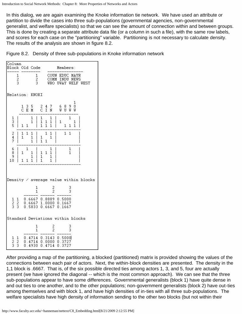
Introduction to Social Network Methods: Chapter 8: More Properties of Networks and Actors
http://www.faculty.ucr.edu/~hanneman/nettext/C8_Embedding.html[8/21/2009 2:12:55 PM]
In this dialog, we are again examining the Knoke information tie network. We have used an attribute orpartition to divide the cases into three sub-populations (governmental agencies, non-governmentalgeneralist, and welfare specialists) so that we can see the amount of connection within and between groups. This is done by creating a separate attribute data file (or a column in such a file), with the same row labels,and scores for each case on the "partitioning" variable. Partitioning is not necessary to calculate density. The results of the analysis are shown in figure 8.2.
Figure 8.2. Density of three sub-populations in Knoke information network
After providing a map of the partitioning, a blocked (partitioned) matrix is provided showing the values of theconnections between each pair of actors. Next, the within-block densities are presented. The density in the1,1 block is .6667. That is, of the six possible directed ties among actors 1, 3, and 5, four are actuallypresent (we have ignored the diagonal -- which is the most common approach). We can see that the threesub-populations appear to have some differences. Governmental generalists (block 1) have quite dense inand out ties to one another, and to the other populations; non-government generalists (block 2) have out-tiesamong themselves and with block 1, and have high densities of in-ties with all three sub-populations. Thewelfare specialists have high density of information sending to the other two blocks (but not within their

Introduction to Social Network Methods: Chapter 8: More Properties of Networks and Actors
http://www.faculty.ucr.edu/~hanneman/nettext/C8_Embedding.html[8/21/2009 2:12:55 PM]
block), and receive more input from governmental than from non-governmental organizations.
The extent to which these simple characterizations of blocks characterize all the individuals within thoseblocks -- essentially the validity of the blocking -- can be assessed by looking at the standard deviationswithin the partitions. The standard deviations measure the lack of homogeneity within the partition, or theextent to which the actors vary.
A social structure in which individuals were highly clustered would display a pattern of high densities on thediagonal, and low densities elsewhere.
table of contents
Reciprocity
With symmetric dyadic data, two actors are either connected, or they are not. Density tells up pretty much allthere is to know.
With directed data, there are four possible dyadic relationships: A and B are not connected, A sends to B, Bsends to A, or A and B send to each other. A common interest in looking at directed dyadic relationships isthe extent to which ties are reciprocated. Some theorists feel that there is an equilibrium tendency towarddyadic relationships to be either null or reciprocated, and that asymmetric ties may be unstable. A networkthat has a predominance of null or reciprocated ties over asymmetric connections may be a more "equal" or"stable" network than one with a predominance of asymmetric connections (which might be more of ahierarchy).
There are (at least) two different approaches to indexing the degree of reciprocity in a population. Considerthe very simple network shown in figure 8.3. Actors A and B have reciprocated ties, actors B and C have anon-reciprocated tie, and actors A and C have no tie.
Figure 8.3. Definitions of reciprocity
What is the prevalence of reciprocity in this network? One approach is to focus on the dyads, and ask whatproportion of pairs have a reciprocated tie between them? This would yield one such tie for three possiblepairs (AB, AC, BC), or a reciprocity rate of .333. More commonly, analysts are concerned with the ratio ofthe number of pairs with a reciprocated tie relative to the number of pairs with any tie. In large populations,usually most actors have no direct ties to most other actors, and it may be more sensible to focus on thedegree of reciprocity among pairs that have any ties. In our simple example, this would yield onereciprocated pair divided by two tied pairs, or a reciprocity rate of .500. The method just described is calledthe dyad method in Network>Cohesion>Reciprocity.
Rather than focusing on actors, we could focus on relations. We could ask, what percentage of all possible

Introduction to Social Network Methods: Chapter 8: More Properties of Networks and Actors
http://www.faculty.ucr.edu/~hanneman/nettext/C8_Embedding.html[8/21/2009 2:12:55 PM]
ties (or "arcs" of the directed graph) are parts of reciprocated structures? Here, two such ties (A to B and Bto A) are a reciprocated structure among the six possible ties (AB, BA, AC, CA, BC, CA) or a reciprocity of.333. Analysts usually focus, instead, on the number of ties that are involved in reciprocal relations relativeto the total number of actual ties (not possible ties). Here, this definition would give us 2 / 3 or .667. Thisapproach is called the arc method in Network>Cohesion>Reciprocity. Here's a typical dialog for using thistool.
Figure 8.4. Dialog for Network>Network Properties>Reciprocity
We've specified the "hybrid" method (the default) which is the same as the dyad approach. Note that it ispossible to block or partition the data by some pre-defined attribute (like in the density example above) toexamine the degree of reciprocity within and between sub-populations. Figure 8.5 shows the results for theKnoke information network.
Figure 8.5. Reciprocity in the Knoke information network
We see that, of all all pairs of actors that have any connection, 53% of the pairs have a reciprocatedconnection. This is neither "high" nor "low" in itself" but does seem to suggest a considerable degree ofinstitutionalized horizontal connection within this organizational population.
The alternative method of "arc" reciprocity (not shown here) yield a result of .6939. That is, of all therelations in the graph, 69% are parts of reciprocated ties.
table of contents
Transitivity
Small group theorists argue that many of the most interesting and basic questions of social structure arisewith regard to triads. Triads allow for a much wider range of possible sets of relations.
With un-directed data, there are four possible types of triadic relations (no ties, one tie, two ties, or all threeties). Counts of the relative prevalence of these four types of relations across all possible triples (that is a"triad census") can give a good sense of the extent to which a population is characterized by "isolation,"

Introduction to Social Network Methods: Chapter 8: More Properties of Networks and Actors
http://www.faculty.ucr.edu/~hanneman/nettext/C8_Embedding.html[8/21/2009 2:12:55 PM]
"couples only," "structural holes" (i.e. where one actor is connected to two others, who are not connected toeach other), or "clusters." UCINET does not have a routine for conducting triad censuses (see Pajek, whichdoes).
With directed data, there are actually 16 possible types of relations among 3 actors), including relationshipsthat exhibit hierarchy, equality, and the formation of exclusive groups (e.g. where two actors connect, andexclude the third). Thus, small group researchers suggest, all of the really fundamental forms of socialrelationships can be observed in triads. Because of this interest, we may wish to conduct a "triad census" foreach actor, and for the network as a whole (again, see Pajek).
In particular, we may be interested in the proportion of triads that are "transitive" (that is, display a type ofbalance where, if A directs a tie to B, and B directs a tie to C, then A also directs a tie to C). Such transitiveor balanced triads are argued by some theorists to be the "equilibrium" or natural state toward which triadicrelationships tend (not all theorists would agree!).
Of the 16 possible types of directed triads, six involve zero, one, or two relations -- and can't displaytransitivity because there are not enough ties to do so. One type with 3 relations (AB, BC, CB) does nothave any ordered triples (AB, BC) and hence can't display transitivity. In three more types of triads, there areordered triples (AB, BC) but the relation between A and C is not transitive. The remaining types of triadsdisplay varying degrees of transitivity.
UCINET does not have extensive algorithms for examining full triad censuses and building more complexmodels based on them (e.g. balance, clusterability, ranked clusters). A more extended treatment of thisapproach, with supporting software is available from Pajek. Nonetheless, the Network>Cohesion>Transitivityalgorithms in UCINET offer some interesting and flexible approaches to characterizing the transitivity oftriads in populations. A typical dialog is shown in figure 8.6.
Figure 8.6. Dialog of Network>Cohesion>Transitivity
The Knoke information network is a binary, directed graph. For data of this type, the default definition oftransitivity (i.e. "Adjacency") is a reasonable approach. This means that we will count the number of timesthat, if we see AB and BC, we also see AC.
Network>Cohesion>Transitivity also provides some alternative definitions of what it means for a triad to betransitive which are useful for valued data.
A strong transitivity is one in which there are connections AB, BC, and AC, and the connection AC is strongerthan the Min value of Strong tie. A weak transitivity is one in which there are connections AB, BC and AC,and AC; the value of AC is less than the threshold for a strong tie, but greater than the threshold Min value ofWeak tie.

Introduction to Social Network Methods: Chapter 8: More Properties of Networks and Actors
http://www.faculty.ucr.edu/~hanneman/nettext/C8_Embedding.html[8/21/2009 2:12:55 PM]
Two other methods are also available. A Euclidean transitivity is defined as a case where AB, BC, and ACare present, and AC has a value less than the sum of AB + BC. A Stochastic transitivity is defined as thecase where AB, BC, and AC are present, and AC is less than the produce AB*BC.
Figure 8.7. Transitivity results for Knoke information network
After performing a census of all possible triads, Network>Cohesion>Transitivity reports that it finds 146transitive (directed) triples. That is, there are 146 cases where, if AB and BC are present, then AC is alsopresent. There are a number of different ways in which we could try to norm this count so that it becomesmore meaningful. One approach is to divide the number of transitive triads by the total number of triads ofall kinds (720). This shows that 20.28% of all triads are transitive. Perhaps more meaningful is to norm thenumber of transitive triads by the number of cases where a single link could complete the triad. That is,norm the number of {AB, BC, AC} triads by the number of {AB, BC, anything} triads. Seen in this way, about2/3 or all relations that could easily be transitive, actually are.
table of contents
Clustering
Watts (1999) and many others have noted that in large, real-world networks (of all kinds of things) there isoften a structural pattern that seems somewhat paradoxical.
On one hand, in many large networks (like, for example, the Internet) the average geodesic distancebetween any two nodes is relatively short. The "6-degrees" of distance phenomenon is an example of this. So, most of the nodes in even very large networks may be fairly close to one another. The average distancebetween pairs of actors in large empirical networks are often much shorter than in random graphs of thesame size.
On the other hand, most actors live in local neighborhoods where most others are also connected to oneanother. That is, in most large networks, a very large proportion of the total number of ties are highly"clustered" into local neighborhoods. That is, the density in local neighborhoods of large graphs tend to bemuch higher than we would expect for a random graph of the same size.
Most of the people we know may also know one another -- seeming to locate us in a very narrow socialworld. Yet, at the same time, we can be at quite short distances to vast numbers of people that we don'tknow at all. The "small world" phenomena -- a combination of short average path lengths over the entiregraph, coupled with a strong degree of "clique-like" local neighborhoods -- seems to have evolvedindependently in many large networks.
We've already discussed one part of this phenomenon. The average geodesic distance between all actors in

Introduction to Social Network Methods: Chapter 8: More Properties of Networks and Actors
http://www.faculty.ucr.edu/~hanneman/nettext/C8_Embedding.html[8/21/2009 2:12:55 PM]
a graph gets at the idea of how close actors are together. The other part of the phenomenon is the tendencytowards dense local neighborhoods, or what is now thought of as "clustering."
One common way of measuring the extent to which a graph displays clustering is to examine the localneighborhood of an actor (that is, all the actors who are directly connected to ego), and to calculate thedensity in this neighborhood (leaving out ego). After doing this for all actors in the whole network, we cancharacterize the degree of clustering as an average of all the neighborhoods.
Figure 8.8 shows the output of Network>Cohesion>Clustering Coefficient as applied to the Knokeinformation network.
Figure 8.8. Network>Cohesion>Clustering Coefficient of Knoke information network
Two alternative measures are presented. The "overall" graph clustering coefficient is simply the average ofthe densities of the neighborhoods of all of the actors. The "weighted" version gives weight to theneighborhood densities proportional to their size; that is, actors with larger neighborhoods get more weight incomputing the average density. Since larger graphs are generally (but not necessarily) less dense thansmaller ones, the weighted average neighborhood density (or clustering coefficient) is usually less than theun-weighted version. In our example, we see that all of the actors are surrounded by local neighborhoodsthat are fairly dense -- our organizations can be seen as embedded in dense local neighborhoods to a fairlyhigh degree. Lest we over-interpret, we must remember that the overall density of the entire graph in thispopulation is rather high (.54). So, the density of local neighborhoods is not really much higher than thedensity of the whole graph. In assessing the degree of clustering, it is usually wise to compare the clustercoefficient to the overall density.
We can also examine the densities of the neighborhoods of each actor, as is shown in figure 8.9.
Figure 8.9. Node level clustering coefficients for Knoke information network
The sizes of each actor's neighborhood is reflected in the number of pairs of actors in it. Actor 6, for examplehas three neighbors, and hence three possible ties. Of these, only one is present -- so actor 6 is not highlyclustered. Actor 8, on the other hand, is in a slightly larger neighborhood (6 neighbors, and hence 15 pairs ofneighbors), but 80% of all the possible ties among these neighbors are present. Actors 8 and 10 areembedded in highly clustered neighborhoods.
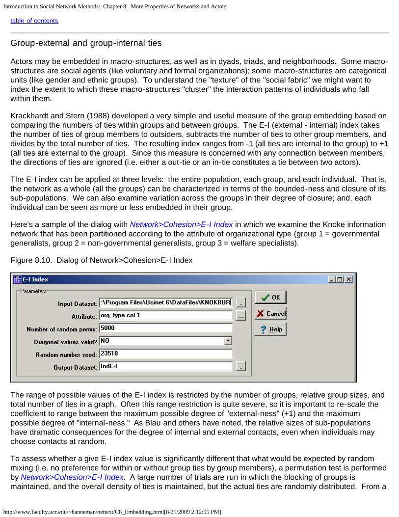
Introduction to Social Network Methods: Chapter 8: More Properties of Networks and Actors
http://www.faculty.ucr.edu/~hanneman/nettext/C8_Embedding.html[8/21/2009 2:12:55 PM]
table of contents
Group-external and group-internal ties
Actors may be embedded in macro-structures, as well as in dyads, triads, and neighborhoods. Some macro-structures are social agents (like voluntary and formal organizations); some macro-structures are categoricalunits (like gender and ethnic groups). To understand the "texture" of the "social fabric" we might want toindex the extent to which these macro-structures "cluster" the interaction patterns of individuals who fallwithin them.
Krackhardt and Stern (1988) developed a very simple and useful measure of the group embedding based oncomparing the numbers of ties within groups and between groups. The E-I (external - internal) index takesthe number of ties of group members to outsiders, subtracts the number of ties to other group members, anddivides by the total number of ties. The resulting index ranges from -1 (all ties are internal to the group) to +1(all ties are external to the group). Since this measure is concerned with any connection between members,the directions of ties are ignored (i.e. either a out-tie or an in-tie constitutes a tie between two actors).
The E-I index can be applied at three levels: the entire population, each group, and each individual. That is,the network as a whole (all the groups) can be characterized in terms of the bounded-ness and closure of itssub-populations. We can also examine variation across the groups in their degree of closure; and, eachindividual can be seen as more or less embedded in their group.
Here's a sample of the dialog with Network>Cohesion>E-I Index in which we examine the Knoke informationnetwork that has been partitioned according to the attribute of organizational type (group 1 = governmentalgeneralists, group 2 = non-governmental generalists, group 3 = welfare specialists).
Figure 8.10. Dialog of Network>Cohesion>E-I Index
The range of possible values of the E-I index is restricted by the number of groups, relative group sizes, andtotal number of ties in a graph. Often this range restriction is quite severe, so it is important to re-scale thecoefficient to range between the maximum possible degree of "external-ness" (+1) and the maximumpossible degree of "internal-ness." As Blau and others have noted, the relative sizes of sub-populationshave dramatic consequences for the degree of internal and external contacts, even when individuals maychoose contacts at random.
To assess whether a give E-I index value is significantly different that what would be expected by randommixing (i.e. no preference for within or without group ties by group members), a permutation test is performedby Network>Cohesion>E-I Index. A large number of trials are run in which the blocking of groups ismaintained, and the overall density of ties is maintained, but the actual ties are randomly distributed. From a

Introduction to Social Network Methods: Chapter 8: More Properties of Networks and Actors
http://www.faculty.ucr.edu/~hanneman/nettext/C8_Embedding.html[8/21/2009 2:12:55 PM]
large number of trials (the default is 5000), a sampling distribution of the numbers of internal and externalties -- under the assumption that ties are randomly distributed -- can be calculated. This samplingdistribution can then be used to assess the frequency with which the observed result would occur bysampling from a population in which ties were randomly distributed.
Let's look first at the results for the graph as a whole, in figure 8.11.
Figure 8.11. E-I index output for the Knoke information network - whole network
The observed block densities are presented first. Since any tie (in or out) is regarded as a tie, the densitiesin this example are quite high. The densities off the main diagonal (out-group ties) appear to be slightly moreprevalent than the densities on the main diagonal (in-group ties).
Next, we see the numbers of internal ties (14, or 22%) and external ties (50, or 78%) that yield a raw (notrescaled) E-I index of +.563. That is, a preponderance of external over internal ties for the graph as a whole. Also shown are the maximum possible numbers of internal and external ties given the group sizes anddensity. Note that, due to these constraints, the result of a preponderance of external ties is not unexpected-- under a random distribution, the E-I index would be expected to have a value of .467, which is not verymuch different from the observed value.
We see that, given the group sizes and density of the graph, the maximum possible value of the index (1.0)and its minimum value (+.25) are both positive. If we re-scale the observed value of the E-I index (.563) to

Introduction to Social Network Methods: Chapter 8: More Properties of Networks and Actors
http://www.faculty.ucr.edu/~hanneman/nettext/C8_Embedding.html[8/21/2009 2:12:55 PM]
fall into this range, we obtain a re-scaled index value of -.167. This suggests, that, given the demographicconstraints and overall density, there is a very modest tendency toward group closure.
The last portion of the results gives the values of the premution-based sampling distribution. Most importanthere is the standard deviation of the sampling distribution of the index, or its standard error (.078). Thissuggests that the value of the raw index is expected to vary by this much from trial to trial (on the average)just by chance. Given this result, we can compare the observed value in our sample (.563) to the expectedvalue (.467) relative to the standard error. The observed difference of about .10 could occur fairly frequentlyjust by sampling variability (p = .203). Most analysts would not reject the null hypothesis that the deviationfrom randomness was not "significant." That is, we cannot be confident that the observed mild bias towardgroup closure is not random variation.
The E-I index can also be calculated for each group and for each individual. These index numbers describethe tendencies toward group closure of each of the groups, and the propensity of each individual to have tieswithin their group. Figure 8.12 displays the results.
Figure 8.12. E-I index output for the Knoke information network - groups and individuals
The first panel of figure 8.12 shows the raw counts of ties within and without each of the three types oforganizations, and the E-I index for each group. Governmental generalists (group 2) appear to be somewhatmore likely to have out-group ties than either of the other sub-populations. The relatively small difference,though, should be treated with considerable caution given the sampling variability (we cannot directly applythe standard error estimate for the whole graph to the results for sub-populations or individuals, but they aresuggestive). We should also note that the E-I results for groups and individuals are in "raw" form, and not"rescaled."
There is considerable variability across individuals in their propensity to in-group ties, as can be seen in thelast panel of the results. Several actors (4, 6, 9) tend toward closure -- having a preponderance of ties withintheir own group; a couple others (10, 1) tend toward a preponderance of ties outside their groups.
table of contents
Krackhardt's graph theoretical dimensions of hierarchy

Introduction to Social Network Methods: Chapter 8: More Properties of Networks and Actors
http://www.faculty.ucr.edu/~hanneman/nettext/C8_Embedding.html[8/21/2009 2:12:55 PM]
Embedding of actors in dyads, triads, neighborhoods, clusters, and groups are all ways in which the socialstructure of a population may display "texture." All of these forms of embedding structures speak to the issueof the "horizontal differentiation" of the population -- separate, but not necessarily ranked or unequalgroupings.
A very common form of embedding of actors in structures, though, does involve unequal rankings. Hierarchies, in which individuals or sub-populations are not only differentiated, but also ranked, areextremely common in social life. The degree of hierarchy in a population speaks to the issue of "verticaldifferentiation."
While we all have an intuitive sense of what it means for a structure to be a hierarchy. Most would agree thatstructures can be "more or less" hierarchical. It is necessary to be quite precise about the meaning of theterm if we are going to build indexes to measure the degree of hierarchy.
Krackhardt (1994) provided an elegant definition of the meaning of hierarchy, and developed measures ofeach of the four component dimensions of the concept that he identified. Krackhardt defines a pure, "idealtypical" hierarchy as an "out-tree" graph. An out-tree graph is a directed graph in which all points areconnected, and all but one node (the "boss") has an in-degree of one. This means that all actors in thegraph (except the ultimate "boss") have a single superior node. The simplest "hierarchy" is a directed linegraph A to B to C to D... More complex hierarchies may have wider, and varying "spans of control" (out-degrees of points).
This very simple definition of the pure type of hierarchy can be deconstructed into four individually necessaryand jointly sufficient conditions. Krackhardt develops index numbers to assess the extent to which each ofthe four dimensions deviates from the pure ideal type of an out-tree, and hence develops four measures ofthe extent to which a given structure resembles the ideal typical hierarchy.
1) Connectedness: To be a pure out-tree, a graph must be connected into a single component -- all actorsare embedded in the same structure. We can measure the extent to which this is not true by looking at theratio of the number of pairs in the directed graph that are reachable relative to the number of ordered pairs. That is, what proportion of actors cannot be reached by other actors? Where a graph has multiplecomponents -- multiple un-connected sub-populations -- the proportion not reachable can be high. If all theactors are connected in the same component, if there is a "unitary" structure, the graph is more hierarchical.
2) Hierarchy: To be a pure out-tree, there can be no reciprocated ties. Reciprocal relations between twoactors imply equal status, and this denies pure hierarchy. We can assess the degree of deviation from purehierarchy by counting the number of pairs that have reciprocated ties relative to the number of pairs wherethere is any tie; that is, what proportion of all tied pairs have reciprocated ties.
3) Efficiency: To be a pure out-tree each node must have an in-degree of one. That is, each actor (exceptthe ultimate boss) has a single boss. This aspect of the idea type is termed "efficiency" because structureswith multiple bosses have un-necessary redundant communication of orders from superiors to subordinates. The amount of deviation from this aspect of the pure out-tree can be measured by counting the differencebetween the actual number of links (minus 1, since the ultimate boss has no boss) and the maximumpossible number of links. The bigger the difference, the greater the inefficiency. This dimension thenmeasures the extent to which actors have a "single boss."
4) Least upper bound (LUB): To be a pure out-tree, each pair of actors (except pairs formed between theultimate boss and others) must have an actor that directs ties to both -- that is, command must be unified. The deviation of a graph from this condition can be measured by counting the numbers of pairs of actors thatdo not have a common boss relative to the number of pairs that could (which depends on the number of

Introduction to Social Network Methods: Chapter 8: More Properties of Networks and Actors
http://www.faculty.ucr.edu/~hanneman/nettext/C8_Embedding.html[8/21/2009 2:12:55 PM]
actors and the span of control of the ultimate boss).
The Network>Cohesion>Krackhardt GTD algorithms calculate indexes of each of the four dimensions, wherehigher scores indicate greater hierarchy. Figure 8.13 shows the results for the Knoke information network.
Figure 8.13. Output of Network>Network Properties>Krackhardt GDT for Knoke information network
The information network does form a single component, as there is at least one actor that can reach allothers. So, the first dimension of pure hierarchy -- that all the actors be embedded in a single structure -- issatisfied. The ties in the information exchange network, though are very likely to be reciprocal (at leastinsofar as they can be, given the limitations of the density). There are a number of nodes that receiveinformation from multiple others, so the network is not "efficient." The least upper bound measure (theextent to which all actors have a boss in common) reports a value of 1.25, which would appear to be out ofrange and, frankly, is a puzzle.
table of contents
Summary
This chapter and the next are concerned with the ways in which networks display "structure" or deviationfrom random connection. In the current chapter, we've approached the same issue of structuring from the"top-down" by looking at patterns of macro-structure in which individuals are embedded in non-randomways. Individuals are embedded (usually simultaneously) in dyads, triads, face-to-face local groups ofneighbors, and larger organizational and categorical social structures. The tools in the current chapterprovide some ways of examining the "texture" of the structuring of the whole population.
In the next chapter we will focus on the same issue of connection and structure from the "bottom-up." Thatis, we'll look at structure from the point of view of the individual "ego."
Taken together, the approaches in chapters 8 and 9 illustrate, again, the "duality" of social structure in whichindividuals make social structures, but do so within a matrix of constraints and opportunities imposed bylarger patterns.
table of contentstable of contents of the book

Chapter 9: Ego networks
http://www.faculty.ucr.edu/~hanneman/nettext/C9_Ego_networks.html[8/21/2009 2:13:17 PM]
Introduction to social network methods
9. Ego networks
This page is part of an on-line text by Robert A. Hanneman (Department of Sociology, University of California, Riverside) and Mark Riddle(Department of Sociology, University of Northern Colorado). Feel free to use and distribute this textbook, with citation. Your comments andsuggestions are very welcome. Send me e-mail.
Contents of chapter 9: Ego networks
IntroductionEgo network data Ego network densityStructural holesBrokerageSummary
Introduction
In the previous chapter we looked at the idea of the amount of "embedding" in whole networks -- loosely: theextent to which actors find themselves in social structures characterized by dense, reciprocal, transitive, strongties. The main theme was to understand and index the extent and nature of the pattern of "constraint" on actorsthat results from the way that they are connected to others. These approaches may tell us some interesting thingsabout the entire population and its sub-populations; but, they don't tell us very much about the opportunities andconstraints facing individuals.
If we want to understand variation in the behavior of individuals, we need to take a closer look at their localcircumstances. Describing and indexing the variation across individuals in the way they are embedded in "local"social structures is the goal of the analysis of ego networks.
We need some definitions.
"Ego" is an individual "focal" node. A network has as many egos as it has nodes. Egos can be persons, groups,organizations, or whole societies.
"Neighborhood" is the collection of ego and all nodes to whom ego has a connection at some path length. In socialnetwork analysis, the "neighborhood" is almost always one-step; that is, it includes only ego and actors that aredirectly adjacent. The neighborhood also includes all of the ties among all of the actors to whom ego has a directconnection. The boundaries of ego networks are defined in terms of neighborhoods.
"N-step neighborhood" expands the definition of the size of ego's neighborhood by including all nodes to whomego has a connection at a path length of N, and all the connections among all of these actors. Neighborhoods ofgreater path length than 1 (i.e. egos adjacent nodes) are rarely used in social network analysis. When we use theterm neighborhood here, we mean the one-step neighborhood.
"In" and "Out" and other kinds of neighborhoods. Most of the analysis of ego networks uses simple graphs (i.e.graphs that are symmetric, and show only connection/not, not direction). If we are working with a directed graph, itis possible to define different kinds of ego-neighborhoods. An "out" neighborhood would include all the actors towhom ties are directed from ego. An "in" neighborhood would include all the actors who sent ties directly to ego. We might want to define a neighborhood of only those actors to whom ego had reciprocated ties. There isn't asingle "right" way to define an ego neighborhood for every research question.
"Strong and weak tie neighborhoods." Most analysis of ego networks uses binary data -- two actors are connected

Chapter 9: Ego networks
http://www.faculty.ucr.edu/~hanneman/nettext/C9_Ego_networks.html[8/21/2009 2:13:17 PM]
or they aren't, and this defines the ego neighborhood. But if we have measured the strength of the relationbetween two actors, and even its valence (positive or negative), we need to make choices about when we aregoing to decide that another actor is ego's neighbor. With ties that are measured as strengths or probabilities, areasonable approach is to define a cut-off value (or, better, explore several reasonable alternatives). Where theinformation about ties includes information about positive/negative, the most common approach is to analyze thepositive tie neighborhood and the negative tie neighborhood separately.
table of contents
Ego network data
Ego network data commonly arise in two ways:
Surveys may be used to collect information on ego networks. We can ask each research subject to identify all ofthe actors to whom they have a connection, and to report to us (as an informant) what the ties are among theseother actors. Alternatively, we could use a two-stage snowball method; first ask ego to identify others to whom egohas a tie, then ask each of those identified about their ties to each of the others identified.
Data collected in this way cannot directly inform us about the overall embeddedness of the networks in apopulation, but it can give us information on the prevalence of various kinds of ego networks in even very largepopulations. When data are collected this way, we essentially have a data structure that is composed of acollection of networks. As the actors in each network are likely to be different people, the networks need to betreated as separate actor-by-actor matrices stored as different data sets (i.e. it isn't a good idea to "stack" themultiple networks in the same data file, because the multiple matrices do not represent multiple relations amongthe same set of actors).
A modification of the survey method can give rise to a multi-plex data structure (that is, a "stack" of actor-by-actormatrices of equal dimension). If we ask each ego to characterize their relation with the occupants of social roles (ora particular occupant of a role), and to also report on the relations among occupants of those roles, we can build"conformable" matrices for each ego. For example, suppose that we asked a number of egos: "do you have amale friend or friends in your classroom?" "Do you have a female friend or friends in your classroom?" and "Areyour male friends, friends of your female friends?" The resulting data for each ego would have three nodes (ego,"male friends," "female friends") and the ties among them. Since each ego's matrix would have the same nodes (inthe sense of social roles, but not individuals) they could be treated as a type of multi-plex data that we will discussmore later on.
The second major way in which ego network data arise is by "extracting" them from regular complete network data. The Data>Extract approach can be used to select a single actor and their ties, but would not include the ties amongthe "alters." The Data>Subgraphs from partitions approach could be used if we had previously identified themembers of a particular ego neighborhood, and stored this as an attribute vector.
More commonly, though, we would want to extract multiple, or even all of the ego networks from a full network tobe stored as separate files. For this task, the Data>Egonet tool is ideal. Here is an example of the dialog for usingthe tool:
Figure 9.1. Dialog for Data>Egonet

Chapter 9: Ego networks
http://www.faculty.ucr.edu/~hanneman/nettext/C9_Ego_networks.html[8/21/2009 2:13:17 PM]
Here we are focusing on ballot proposition campaigns in California that are connected by having donors in common(i.e. CA_Props is a proposition-by-proposition valued matrix). We've said that we want to extract a network thatincludes the 3rd, 11th, 17th, and 19th rows/columns, and all the nodes that are connected to any of these actors. More commonly, we might select a single "ego." The list of focal nodes can be provided either as an attribute file,by typing in the list of row numbers, or by selecting the node labels of the desired actors.
A picture of part of the resulting data, stored as a new file called "Neighbor_example" is shown in figure 9.2.
Figure 9.2. (Partial) output of Data>Egonet
Extracting sub-graphs, based on a focal actor or set of actors (e.g. "elites") can be a very useful way of looking at apart of a whole network, or the condition of an individual actor. The Data>Egonet tool is helpful for creating datasets that are good for graphing and separate analysis -- particularly when the networks in which the focalactor/actors are embedded are quite large.
It is not necessary, however, to create separate ego-network datasets for each actor to be analyzed. Theapproaches to analysis that we'll review below generate output for the first-order ego network of every node in adataset. For small datasets, there is often no need to extract separate ego networks.
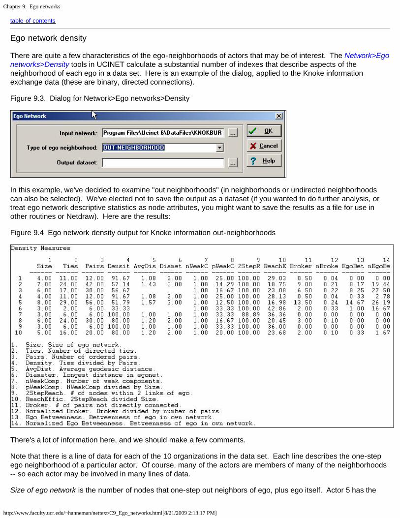
Chapter 9: Ego networks
http://www.faculty.ucr.edu/~hanneman/nettext/C9_Ego_networks.html[8/21/2009 2:13:17 PM]
table of contents
Ego network density
There are quite a few characteristics of the ego-neighborhoods of actors that may be of interest. The Network>Egonetworks>Density tools in UCINET calculate a substantial number of indexes that describe aspects of theneighborhood of each ego in a data set. Here is an example of the dialog, applied to the Knoke informationexchange data (these are binary, directed connections).
Figure 9.3. Dialog for Network>Ego networks>Density
In this example, we've decided to examine "out neighborhoods" (in neighborhoods or undirected neighborhoodscan also be selected). We've elected not to save the output as a dataset (if you wanted to do further analysis, ortreat ego network descriptive statistics as node attributes, you might want to save the results as a file for use inother routines or Netdraw). Here are the results:
Figure 9.4 Ego network density output for Knoke information out-neighborhoods
There's a lot of information here, and we should make a few comments.
Note that there is a line of data for each of the 10 organizations in the data set. Each line describes the one-stepego neighborhood of a particular actor. Of course, many of the actors are members of many of the neighborhoods-- so each actor may be involved in many lines of data.
Size of ego network is the number of nodes that one-step out neighbors of ego, plus ego itself. Actor 5 has the

Chapter 9: Ego networks
http://www.faculty.ucr.edu/~hanneman/nettext/C9_Ego_networks.html[8/21/2009 2:13:17 PM]
largest ego network, actors 6, 7, and 9 have the smallest networks.
Number of directed ties is the number of connections among all the nodes in the ego network. Among the fouractors in ego 1's network, there are 11 ties.
Number of ordered pairs is the number of possible directed ties in each ego network. In node 1's network there arefour actors, so there are 4*3 possible directed ties.
Density is, as the output says, the number of ties divided by the number of pairs. That is, what percentage of allpossible ties in each ego network are actually present? Note that actor 7 and 9 live in neighborhoods where allactors send information to all other actors; they are embedded in very dense local structures. The welfare rightsorganization (node 6) lives in a small world where the members are not tightly connected. This kind of difference inthe constraints and opportunities facing actors in their local neighborhoods may be very consequential.
Average geodesic distance is the mean of the shortest path lengths among all connected pairs in the ego network. Where everyone is directly connected to everyone (e.g. node 7 and 9) this distance is one. In our example, thelargest average path length for connected neighbors is for actor 5 (average distances among members of theneighborhood is 1.57).
Diameter of an ego network is the length of the longest path between connected actors (just as it is for anynetwork). The idea of a network diameter, is to index the span or extensiveness of the network -- how far apart arethe two furthest actors. In the current example, they are not very far apart in the ego networks of most actors.
In addition to these fairly basic and reasonably straight-forward measures, the output provides some more exoticmeasures that get at some quite interesting ideas about ego neighborhoods that have been developed by anumber of social network researchers.
Number of weak components. A weak component is the largest number of actors who are connected,disregarding the direction of the ties (a strong component pays attention to the direction of the ties for directeddata). If ego was connected to A and B (who are connected to one another), and ego is connected to C and D(who are connected to one another), but A and B are not connected in any way to C and D (except by way ofeveryone being connected to ego) then there would be two "weak components" in ego's neighborhood. In ourexample, there are no such cases -- each ego is embedded in a single component neighborhood. That is, thereare no cases where ego is the only connection between otherwise dis-joint sets of actors.
Number of weak components divided by size. The likelihood that there would be more than one weak componentsin ego's neighborhood would be a function of neighborhood size if connections were random. So, to get a sense ofwhether ego's role in connecting components is "unexpected" given the size of their network, it is useful tonormalize the count of components by size. In our example, since there are no cases of multiple components, thisis a pretty meaningless exercise.
Two-step reach goes beyond ego's one-step neighborhood to report the percentage of all actors in the wholenetwork that are within two directed steps of ego. In our example, only node 7 cannot get a message to all otheractors within "friend-of-a-friend" distance.
Reach efficiency (two-step reach divided by size) norms the two-step reach by dividing it by size. The idea here is:how much (non-redundant) secondary contact to I get for each unit of primary contact? If reach efficiency is high,then I am getting a lot of "bang for my buck" in reaching a wider network for each unit of effort invested inmaintaining a primary contact. If my neighbors, on the average, have few contacts that I don't have, I have lowefficiency.
Brokerage (number of pairs not directly connected). The idea of brokerage (more on this, below) is that ego is the"go-between" for pairs of other actors. In an ego network, ego is connected to every other actor (by definition). Ifthese others are not connected directly to one another, ego may be a "broker" ego falls on a the paths between theothers. One item of interest is simply how much potential for brokerage there is for each actor (how many times

Chapter 9: Ego networks
http://www.faculty.ucr.edu/~hanneman/nettext/C9_Ego_networks.html[8/21/2009 2:13:17 PM]
pairs of neighbors in ego's network are not directly connected). In our example, actor number 5, who is connectedto almost everyone, is in a position to broker many connections.
Normalized brokerage (brokerage divided by number of pairs) assesses the extent to which ego's role is that ofbroker. One can be in a brokering position a number of times, but this is a small percentage of the total possibleconnections in a network (e.g. the network is large). Given the large size of actor 5's network, the relativefrequency with which actor 5 plays the broker role is not so exceptional.
Betweenness is an aspect of the larger concept of "centrality." A later chapter provides a more in-depth treatmentof the concept and its application to whole networks. For the moment, though, it' pretty easy to get the basic idea. Ego is "between" two other actors if ego lies on the shortest directed path from one to the other. The egobetweenness measure indexes the percentage of all geodesic paths from neighbor to neighbor that pass throughego.
Normalized Betweenness compares the actual betweenness of ego to the maximum possible betweenness inneighborhood of the size and connectivity of ego's. The "maximum" value for betweenness would be achievedwhere ego is the center of a "star" network; that is, no neighbors communicate directly with one another, and alldirected communications between pairs of neighbors go through ego.
The ideas of "brokerage" and "betweenness" are slightly differing ways of indexing just how "central" or "powerful"ego is within their own neighborhood. This aspect of how an actor's embedding may provide them with strategicadvantage has received a great deal of attention. The next two sections, on "structural holes" and "brokerage"elaborate on ways of looking at positional opportunity and constraint of individual actors.
table of contents
Structural holes
In several important works, Ronald Burt coined and popularized the term "structural holes" to refer to some veryimportant aspects of positional advantage/disadvantage of individuals that result from how they are embedded inneighborhoods. Burt's formalization of these ideas, and his development of a number of measures (including thecomputer program Structure, that provides these measures and other tools) has facilitated a great deal of furtherthinking about how and why the ways that an actor is connected affect their constraints and opportunities, andhence their behavior.
The basic idea is simple, as good ideas often are.
Imagine a network of three actors (A, B, and C), in which each is connected to each of the others as in figure 9.5.
Figure 9.5. Three actor network with no structural holes
Let's focus on actor A (of course, in this case, the situations of B and C are identical in this particular network). Suppose that actor A wanted to influence or exchange with another actor. Assume that both B and C may havesome interest in interacting or exchanging, as well. Actor A will not be in a strong bargaining position in thisnetwork, because both of A's potential exchange partners (B and C) have alternatives to treating with A; they could
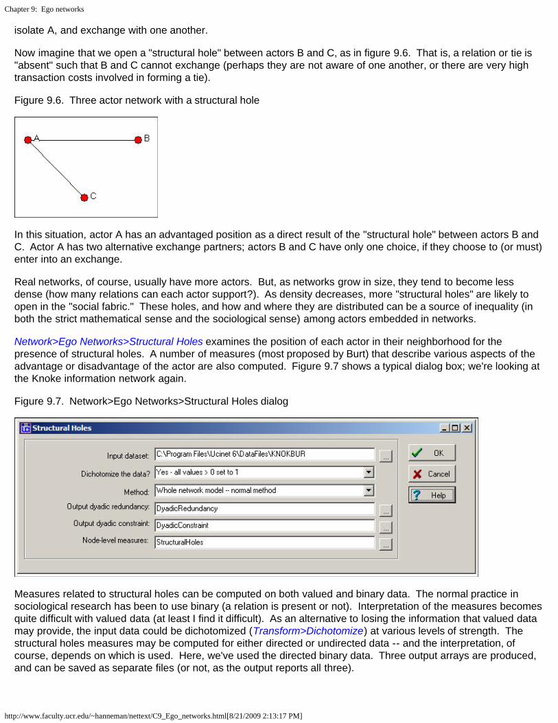
Chapter 9: Ego networks
http://www.faculty.ucr.edu/~hanneman/nettext/C9_Ego_networks.html[8/21/2009 2:13:17 PM]
isolate A, and exchange with one another.
Now imagine that we open a "structural hole" between actors B and C, as in figure 9.6. That is, a relation or tie is"absent" such that B and C cannot exchange (perhaps they are not aware of one another, or there are very hightransaction costs involved in forming a tie).
Figure 9.6. Three actor network with a structural hole
In this situation, actor A has an advantaged position as a direct result of the "structural hole" between actors B andC. Actor A has two alternative exchange partners; actors B and C have only one choice, if they choose to (or must)enter into an exchange.
Real networks, of course, usually have more actors. But, as networks grow in size, they tend to become lessdense (how many relations can each actor support?). As density decreases, more "structural holes" are likely toopen in the "social fabric." These holes, and how and where they are distributed can be a source of inequality (inboth the strict mathematical sense and the sociological sense) among actors embedded in networks.
Network>Ego Networks>Structural Holes examines the position of each actor in their neighborhood for thepresence of structural holes. A number of measures (most proposed by Burt) that describe various aspects of theadvantage or disadvantage of the actor are also computed. Figure 9.7 shows a typical dialog box; we're looking atthe Knoke information network again.
Figure 9.7. Network>Ego Networks>Structural Holes dialog
Measures related to structural holes can be computed on both valued and binary data. The normal practice insociological research has been to use binary (a relation is present or not). Interpretation of the measures becomesquite difficult with valued data (at least I find it difficult). As an alternative to losing the information that valued datamay provide, the input data could be dichotomized (Transform>Dichotomize) at various levels of strength. Thestructural holes measures may be computed for either directed or undirected data -- and the interpretation, ofcourse, depends on which is used. Here, we've used the directed binary data. Three output arrays are produced,and can be saved as separate files (or not, as the output reports all three).

Chapter 9: Ego networks
http://www.faculty.ucr.edu/~hanneman/nettext/C9_Ego_networks.html[8/21/2009 2:13:17 PM]
The results are shown in figure 9.8, and need a bit of explanation.
Figure 9.8. Structural holes results for the Knoke information exchange network
Dyadic redundancy means that ego's tie to alter is "redundant." If A is tied to both B and C, and B is tied to C (as infigure 9.5) A's tie to B is redundant, because A can influence B by way of C. The dyadic redundancy measurecalculates, for each actor in ego's neighborhood, how many of the other actors in the neighborhood are also tied tothe other. The larger the proportion of others in the neighborhood who are tied to a given "alter," the more"redundant" is ego's direct tie. In the example, we see that actor 1's (COUN) tie to actor 2 (COMM) is largelyredundant, as 72% of ego's other neighbors also have ties with COMM. Actors that display high dyadicredundancy are actors who are embedded in local neighborhoods where there are few structural holes.
Dyadic constraint is an measure that indexes the extent to which the relationship between ego and each of thealters in ego's neighborhood "constrains" ego. A full description is given in Burt's 1992 monograph, and theconstruction of the measure is somewhat complex. At the core though, A is constrained by its relationship with B tothe extent that A does not have many alternatives (has few other ties except that to B), and A's other alternativesare also tied to B. If A has few alternatives to exchanging with B, and if those alternative exchange partners arealso tied to B, then B is likely to constrain A's behavior. In our example constraint measures are not very large, asmost actors have several ties. COMM and MAYR are, however, exerting constraint over a number of others, and

Chapter 9: Ego networks
http://www.faculty.ucr.edu/~hanneman/nettext/C9_Ego_networks.html[8/21/2009 2:13:17 PM]
are not very constrained by them. This situation arises because COMM and MAYR have considerable numbers ofties, and many of the actors to whom they are tied do not have many independent sources of information.
Effective size of the network (EffSize) is the number of alters that ego has, minus the average number of ties thateach alter has to other alters. Suppose that A has ties to three other actors. Suppose that none of these three hasties to any of the others. The effective size of ego's network is three. Alternatively, suppose that A has ties to threeothers, and that all of the others are tied to one another. A's network size is three, but the ties are "redundant"because A can reach all three neighbors by reaching any one of them. The average degree of the others in thiscase is 2 (each alter is tied to two other alters). So, the effective size of the network is its actual size (3), reducedby its redundancy (2), to yield an efficient size of 1.
Efficiency (Efficie) norms the effective size of ego's network by its actual size. That is, what proportion of ego's tiesto its neighborhood are "non-redundant." The effective size of ego's network may tell us something about ego'stotal impact; efficiency tells us how much impact ego is getting for each unit invested in using ties. An actor can beeffective without being efficient; and and actor can be efficient without being effective.
Constraint (Constra) is a summary measure that taps the extent to which ego's connections are to others who areconnected to one another. If ego's potential trading partners all have one another as potential trading partners, egois highly constrained. If ego's partners do not have other alternatives in the neighborhood, they cannot constrainego's behavior. The logic is pretty simple, but the measure itself is not. It would be good to take a look at Burt's1992 Structural Holes. The idea of constraint is an important one because it points out that actors who have manyties to others may actually lose freedom of action rather than gain it -- depending on the relationships among theother actors.
Hierarchy (Hierarc) is another quite complex measure that describes the nature of the constraint on ego. If thetotal constraint on ego is concentrated in a single other actor, the hierarchy measure will have a higher value. If theconstraint results more equally from multiple actors in ego's neighborhood, hierarchy will be less. The hierarchymeasure, in itself, does not assess the degree of constraint. But, among whatever constraint there is on ego, itmeasures the important property of dependency -- inequality in the distribution of constraints on ego across thealters in its neighborhood.
table of contents
Brokerage
Burt's approach to understanding how the way that an actor is embedded in its neighborhood is very useful inunderstanding power, influence, and dependency effects. We'll examine some similar ideas in the chapter oncentrality. Burt's underlying approach is that of the rational individual actor who may be attempting to maximizeprofit or advantage by modifying the way in which they are embedded. The perspective is decidedly "neo-classical."
Fernandez and Gould also examined the ways in which actor's embedding might constrain their behavior. Theseauthors though, took a quite different approach; they focus on the roles that ego plays in connecting groups. Thatis, Fernandez and Gould's "brokerage" notions examine ego's relations with its neighborhood from the perspectiveof ego acting as an agent in relations among groups (though, as a practical matter, the groups in brokerageanalysis can be individuals).
To examine the brokerage roles played by a given actor, we find every instance where that actor lies on thedirected path between two others. So, each actor may have many opportunities to act as a "broker." For each oneof the instances where ego is a "broker," we examine which kinds of actors are involved. That is, what are thegroup memberships of each of the three actors? There are five possible combinations.
In figure 9.9, the ego who is "brokering" (node B), and both the source and destination nodes (A and C) are allmembers of the same group. In this case, B is acting as a "coordinator" of actors within the same group as itself.
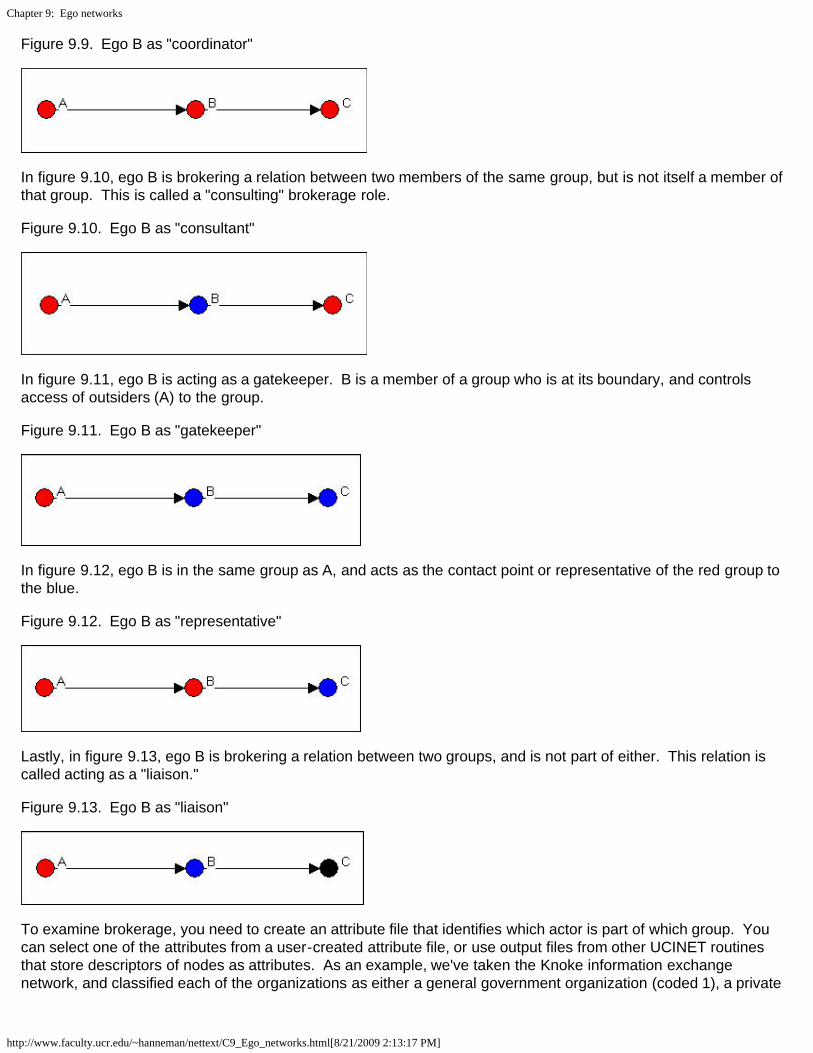
Chapter 9: Ego networks
http://www.faculty.ucr.edu/~hanneman/nettext/C9_Ego_networks.html[8/21/2009 2:13:17 PM]
Figure 9.9. Ego B as "coordinator"
In figure 9.10, ego B is brokering a relation between two members of the same group, but is not itself a member ofthat group. This is called a "consulting" brokerage role.
Figure 9.10. Ego B as "consultant"
In figure 9.11, ego B is acting as a gatekeeper. B is a member of a group who is at its boundary, and controlsaccess of outsiders (A) to the group.
Figure 9.11. Ego B as "gatekeeper"
In figure 9.12, ego B is in the same group as A, and acts as the contact point or representative of the red group tothe blue.
Figure 9.12. Ego B as "representative"
Lastly, in figure 9.13, ego B is brokering a relation between two groups, and is not part of either. This relation iscalled acting as a "liaison."
Figure 9.13. Ego B as "liaison"
To examine brokerage, you need to create an attribute file that identifies which actor is part of which group. Youcan select one of the attributes from a user-created attribute file, or use output files from other UCINET routinesthat store descriptors of nodes as attributes. As an example, we've taken the Knoke information exchangenetwork, and classified each of the organizations as either a general government organization (coded 1), a private

Chapter 9: Ego networks
http://www.faculty.ucr.edu/~hanneman/nettext/C9_Ego_networks.html[8/21/2009 2:13:17 PM]
non-welfare organization (coded 2), or an organizational specialist (coded 3). Figure 9.14 shows the attribute (orpartition) as we created it using the UCINET spreadsheet editor.
Figure 9.14. Partition vector for Knoke information exchange
Using the network data set and the attribute vector we just created, we can run Network>EgoNetworks>Brokerage, as shown in figure 9.15.
The option "unweighted" needs a little explanation. Suppose that actor B was brokering a relation between actorsA and C, and was acting as a "liaison." In the unweighted approach, this would count as one such relation for actorB. But, suppose that there was some other actor D who also was acting as a liaison between A and C. In the"weighted" approach, both B and D would get 1/2 of the credit for this role; in the unweighted approach, both B andD would get full credit. Generally, if we are interested in ego's relations, the unweighted approach would be used. If we were more interested in group relations, a weighted approach might be a better choice.
The output produced by Network>Ego Networks>Brokerage is quite extensive. We'll break it up into a few partsand discuss them separately. The first piece of the output (figure 9.16) is a census of the number of times thateach actor serves in each of the five roles.
Figure 9.16. Unnormalized brokerage scores for Knoke information network

Chapter 9: Ego networks
http://www.faculty.ucr.edu/~hanneman/nettext/C9_Ego_networks.html[8/21/2009 2:13:17 PM]
The actors have been grouped together into "partitions" for presentation; actors 1, 3, and 5, for example, form thefirst type of organization. Each row counts the raw number of times that each actor plays each of the five roles inthe whole graph. Two actors (5 and 2) are the main sources of inter-connection among the three organizationalpopulations. Organizations in the third population (6, 8, 9, 10), the welfare specialists, have overall low rates ofbrokerage. Organizations in the first population (1, 3, 5), the government organizations seem to be more heavilyinvolved in liaison than other roles. Organizations in the second population (2, 4, 7), non-governmental generalistsplay more diverse roles. Overall, there is very little coordination within each of the populations.
We might also be interested in how frequently each actor is involved in relations among and within each of thegroups. Figure 9.17 shows these results for the first two nodes.
Figure 9.17. Group-to-group brokerage map
We see that actor 1 (who is in group 1) plays no role in connections from group 1 to itself or the other groups (i.e.the zero entries in the first row of the matrix). Actor 1 does, however, act as a "liaison" in making a connection fromgroup 2 to group 3. Actor 1 also acts as a "consultant" in connecting a member of group 3 to another member ofgroup 3. The very active actor 2 does not broker relations within group 2, but is heavily involved in ties in bothdirections of all three groups to one another, and relations among members of groups 1 and 3.
These two descriptive maps can be quite useful in characterizing the "role" that each ego is playing in the relationsamong groups by way of their inclusion in its local neighborhood. These roles may help us to understand how eachego may have opportunities and constraints in access to the resources of the social capital of groups, as well asindividuals. The overall maps also inform us about the degree and form of cohesion within and between thegroups.
There may be some danger of "over interpreting" the information about individuals brokerage roles as representingmeaningful acts of "agency." In any population in which there are connections, partitioning will produce brokerage -- even if the partitions are not meaningful, or even completely random. Can we have any confidence that the

Chapter 9: Ego networks
http://www.faculty.ucr.edu/~hanneman/nettext/C9_Ego_networks.html[8/21/2009 2:13:17 PM]
patterns we are seeing in real data are actually different from a random result?
In Figure 9.18, we see the number of relations of each type that would be expected by pure random processes. We ask: what if actors were assigned to groups as we specify, and each actor has the same number of ties toother actors that we actually observe; but, the ties are distributed at random across the available actors? What ifthe pattern of roles was generated entirely by the number of groups of various sizes, rather than representingefforts by the actors to deliberately construct their neighborhoods to deal with the constraints and opportunities ofgroup relations?
Figure 9.18. Expected values under random assignment
If we examine the actual brokerage relative to this random expectation, we can get a better sense of which parts ofwhich actors roles are "significant." That is, occur much more frequently than we would expect in a worldcharacterized by groups, but random relations among them.
Figure 9.19. Normalized brokerage scores
The normalized brokerage scores in this example need to be treated with a little caution. As with most "statistical"approaches, larger samples (more actors) produce more stable and meaningful results. Since our network doesnot contain large numbers of relations, and does not have high density, there are many cases where the expectednumber of relations is small, and finding no such relations empirically is not surprising. Both actor 2 and actor 5,who do broker many relations, do not have profiles that differ greatly from what we would expect by chance. Thelack of large deviations from expected values suggests that we might want to have a good bit of caution ininterpreting our seemingly interesting descriptive data as being highly "significant."
table of contents
Summary

Chapter 9: Ego networks
http://www.faculty.ucr.edu/~hanneman/nettext/C9_Ego_networks.html[8/21/2009 2:13:17 PM]
In this chapter we've taken another look at the notion of embedding; this time, our focus has been on the individualactor, rather than the network as a whole.
The fundamental idea here is that the ways in which individuals are attached to macro-structures is often by way oftheir local connections. It is the local connections that most directly constrain actors, and provide them with accessto opportunities. Examining the ego-networks of individuals can provide insight into why one individual'sperceptions, identity, and behavior differ from another's. Looking at the demography of ego networks in a wholepopulation can tell us a good bit about its differentiation and cohesion - from a micro point of view.
In the next several chapters we will examine additional concepts and algorithms that have been developed in socialnetwork analysis to describe important dimensions of the ways in which individuals and structures interact. We'llstart with one of the most important, but also most troublesome, concepts: power.
table of contentstable of contents of the book