Introduction to ScaLAPACK. 2 ScaLAPACK ScaLAPACK is for solving dense linear systems and computing eigenvalues for dense matrices

Introduction to ScaLAPACK

2

ScaLAPACK

• ScaLAPACK is for solving dense linear systems and computing eigenvalues for dense matrices

3

ScaLAPACK

• Scalable Linear Algebra PACKage

• Developing team from University of Tennessee, University of California Berkeley, ORNL, Rice U.,UCLA, UIUC etc.

• Support in Commercial Packages– NAG Parallel Library – IBM PESSL – CRAY Scientific Library – VNI IMSL – Fujitsu, HP/Convex, Hitachi, NEC

4

Description

• A Scalable Linear Algebra Package (ScaLAPACK)

• A library of linear algebra routines for MPP and NOW machines

• Language : Fortran

• Dense Matrix Problem Solvers – Linear Equations – Least Squares – Eigenvalue

5

Technical Information

• ScaLAPACK web page– http://www.netlib.org/scalapack

• ScaLAPACK User’s Guide

• Technical Working Notes– http://www.netlib.org/lapack/lawn

6

Packages

• LAPACK – Routines are single-PE Linear Algebra solvers,

utilities, etc.

• BLAS – Single-PE processor work-horse routines

(vector, vector-matrix & matrix-matrix)

• PBLAS – Parallel counterparts of BLAS. Relies on

BLACS for blocking and moving data.

7

Packages (cont.)

• BLACS – Constructs 1-D & 2-D processor grids for

matrix decomposition and nearest neighbor communication patterns. Uses message passing libraries (MPI, PVM, MPL, NX, etc) for data movement.

8

Dependencies & Parallelismof Component Packages

BLAS

LAPACK

MPI, PVM,...

BLACS

PBLAS

ScaLAPACK

Serial Parallel

9

Data Partitioning

• Initialize BLACS routines– Set up 2-D mesh (mp, np)– Set (CorR) Column or Row Major Order– Call returns context handle (icon)– Get row & column through gridinfo

(myrow,mycol)

• blacs_gridinit( icon, CorR, mp, np )

• blacs_gridinfo( icon, mp, np, myrow, mycol)

10

Data Partitioning (cont.)

• Block-cyclic Array Distribution.– Block: (groups of sequential elements)– Cyclic: (round-robin assignment to PEs)

• Example 1-D Partitioning: – Global 9-element array distributed on a 3-PE

grid with 2 element blocks: block(2)-cyclic(3)

11

Block-Cyclic Partitioning

11 12 13 14 15 16 17 18 19

15 1611 12 17 18 13 14 19

Block-Cyclic Partitioning Block size = 2, Cyclic on 3-PE Grid

15 1611 12 17 18 13 14 19

PE 0 PE 1 PE 2

0 2

2 34 51

Global Array

Local Arrays

1 Partioned Array often shown by this type of grid map

0Grid Row

Indicates sequence of cyclic distribution.

12

2-D Partitioning

• Example 2-D Partitioning– A(9,9) mapped onto PE(2,3) grid block(2,2)– Use 1-D example to distribute column elements

in each row, a block(2)-cyclic(3) distribution.– Assign rows to first PE dimension by block(2)-

cyclic(2) distribution.

13

11

21

31

41

5161

71

81

91

12

22

32

425262

72

82

92

13 14 15 16 17 18 1923 24 25 26 27 28 29

33 34 35 36 37 38 39

43 44 45 46 47 48 495453 55 56 57 58 59

63 64 65 66 67 68 69

73 74 75 76 77 78 79

83 84 85 86 87 88 89

9593 94 96 97 98 99

11

21

12

22

13 1423 24

15 16

25 26

17 18

27 281929

31

41

32

42

51

615262

71

81

72

82

91 92

33 34

43 44

93 94

73 74

83 84

35 36

45 46

37 38

47 48

39

49

545363 64

55 56

65 6657 58

67 685969

75 76

85 86

77 7887 88

7989

95 9697 98 99

Global Matrix (9x9) Block Size =2x2 Cyclic on 2x3 PE Grid

Global Matrix

PE (0,0) PE (0,1) PE (0,2)

PE (1,0) PE (1,1) PE (1,2)

14

11

21

12

22

13 14

23 24

15 16

25 26

17 18

27 28

19

29

31

41

32

42

51

615262

71

81

72

82

91 92

33 34

43 44

93 94

73 74

83 84

35 36

45 46

37 38

47 48

39

49

545363 64

55 56

65 6657 58

67 685969

75 76

85 86

77 78

87 88

79

89

95 9697 98 99

35 36

45 4675 76

85 86

31

41

32

4271

81

72

82

37 38

47 4877 78

87 88

33 34

43 4473 74

83 84

39

4979

89

15 16

25 26

55 56

65 66

95 96

11

21

12

22

17 18

27 28

51

615262

91 92

57 58

67 68

97 98

13 14

23 24

19

29

93 94

545363 64

5969

99

2 x 3 Processor Grid

PE (0,0) PE (0,1) PE (0,2)

PE (1,0) PE (1,1) PE (1,2)

0 1 2

0

1

Partitioned Array

15

Syntax for descinit

OUT idesc DescriptorIN m Row Size (Global)IN n Column Size (Global)IN mb Row Block SizeIN nb Column SizeIN i Starting Grid RowIN j Starting Grid ColumnIN icon BLACS contextIN mla Leading Dimension of Local MatrixOUT ier Error number

The starting grid location is usually (i=0,j=0).

IorO arg Description

descinit(idesc, m,n, mb,nb, i,j, icon, mla, ier)

16

Application Program Interfaces (API)

• Drivers– Solves a Complete Problem

• Computational Components– Performs Tasks: LU factorization, etc.

• Auxiliary Routines– Scaling, Matrix Norm, etc.

• Matrix Redistribution/Copy Routine– Matrix on PE grid1 -> Matrix on PE grid2

17

API (cont..)

• Prepend LAPACK equivalent names with P.

PXYYZZZComputation Performed

Matrix Type

Data Types

Data Type real double cmplx dble cmplx

X S D C Z

18

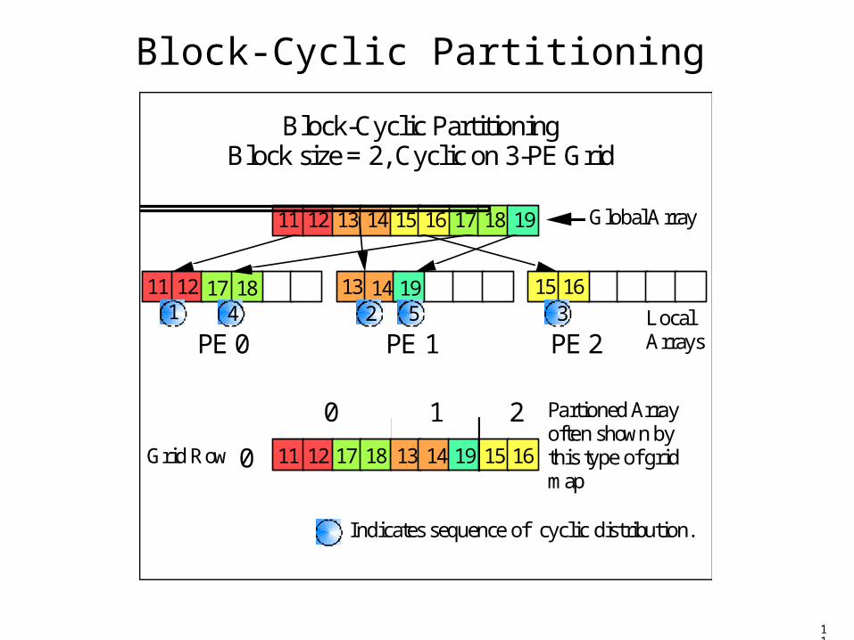
Matrix Types (YY) PXYYZZZ

DB General Band (diagonally dominant-like) DT general Tridiagonal (Diagonally dominant-like) GB General Band GE GEneral matrices (e.g., unsymmetric, rectangular, etc.) GG General matrices, Generalized problem HE Complex Hermitian OR Orthogonal Real PB Positive definite Banded (symmetric or Hermitian) PO Positive definite (symmetric or Hermitian) PT Positive definite Tridiagonal (symmetric or Hermitian) ST Symmetric Tridiagonal Real SY SYmmetric TR TRiangular (possibly quasi-triangular) TZ TrapeZoidal UN UNitary complex

19

Routine types

SL Linear Equations (SVX*)

SV LU Solver

VD Singular Value

EV Eigenvalue (EVX**)

GVX Generalized Eigenvalue

*Estimates condition numbers. *Provides Error Bounds. *Equilibrates System. **Selected Eigenvalues

Drivers (ZZZ) PXYYZZZ

20

Rules of Thumb

• Use a square processor grid, mp=np

• Use block size 32 (Cray) or 64– for efficient matrix multiply

• Number of PEs to use = MxN/10**6

• Bandwith/node (MB/sec) > peak rate (MFLOPS)/10

• Latency < 500 usecs

• Use vendor’s BLAS

21

Example program: Linear Equation Solution Ax=b (page 1)

program Sample_ScaLAPACK_programimplicit noneinclude "mpif.h"REAL :: A ( 1000 , 1000) REAL, DIMENSION(:,:), ALLOCATABLE :: A_local INTEGER, PARAMETER :: M_A=1000, N_A=1000 INTEGER :: DESC_A(1:9) REAL, DIMENSION(:,:), ALLOCATABLE :: b_local REAL :: b( 1000,1 ) INTEGER, PARAMETER :: M_B=1000, N_B=1 INTEGER :: DESC_b(1:9) ,i,jINTEGER :: ldb_y INTEGER :: ipiv(1:1000),info INTEGER :: myrow,mycol !row and column # of PE on PE grid INTEGER :: ictxt !context handle.....like MPIcommunicator INTEGER :: lda_y,lda_x ! leading dimension of local array A(@)! row and column # of PE gridINTEGER, PARAMETER :: nprow=2, npcol=2!! RSRC...the PE row that owns the first row of A! CSRC...the PE column that owns the first column of A

22

Example program (page 2)INTEGER, PARAMETER :: RSRC = 0, CSRC = 0INTEGER, PARAMETER :: MB = 32, NB=32!! iA...the global row index of A, which points to the beginning !of submatrix that will be operated on.! INTEGER, PARAMETER :: iA = 1, jA = 1INTEGER, PARAMETER :: iB = 1, jB = 1REAL :: starttime, endtimeINTEGER :: taskid,numtask,ierr!**********************************! NOTE: ON THE NPACI MACHINES DO NOT NEED TO CALL INITBUFF! ON OTHER MACHINES YOU MAY NEED TO CALL INITBUFF!*************************************! ! This is where you should define any other variables! INTEGER, EXTERNAL :: NUMROC!! Initialization of the processor grid. This routine! must be called! ! start MPI initialization routines

23

Example program (page 3)CALL MPI_INIT(ierr)CALL MPI_COMM_RANK(MPI_COMM_WORLD,taskid,ierr)CALL MPI_COMM_SIZE(MPI_COMM_WORLD,numtask,ierr)! start timing call on 0,0 processorIF (taskid==0) THEN starttime =MPI_WTIME()END IFCALL BLACS_GET(0,0,ictxt) CALL BLACS_GRIDINIT(ictxt,'r',nprow,npcol)!! This call returns processor grid information that will be ! used to distribute the global array! CALL BLACS_GRIDINFO(ictxt, nprow, npcol, myrow, mycol )!! define lda_x and lda_y with numroc! lda_x...the leading dimension of the local array storing the ! ........local blocks of the distributed matrix A!lda_x = NUMROC(M_A,MB,myrow,0,nprow)

lda_y = NUMROC(N_A,NB,mycol,0,npcol) !! resizing A so don't waste space!

24

Example program (page 4)

ALLOCATE( A_local (lda_x,lda_y)) if (N_B < NB )then ALLOCATE( b_local(lda_x,N_B) )else ldb_y = NUMROC(N_B,NB,mycol,0,npcol) ALLOCATE( b_local(lda_x,ldb_y) ) end if!! defining global matrix A!do i=1,1000 do j = 1, 1000

if (i==j) then A(i,j) = 1000.0*i*jelse A(i,j) = 10.0*(i+j)end if

end doend do! defining the global array bdo i = 1,1000 b(i,1) = 1.0end do!

25


! subroutine setarray maps global array to local arrays!! YOU MUST HAVE DEFINED THE GLOBAL MATRIX BEFORE THIS POINT!CALL SETARRAY(A,A_local,b,b_local,myrow,mycol , lda_x,lda_y )!! initialize descriptor vector for scaLAPACK !CALL DESCINIT(DESC_A,M_A,N_A,MB,NB,RSRC,CSRC,ictxt,lda_x,info)

CALL DESCINIT(DESC_b,M_B,N_B,MB,N_B,RSRC,CSRC,ictxt,lda_x,info) ! ! call scaLAPACK routines!

CALL PSGESV( N_A,1,A_local,iA,jA, DESC_A,ipiv,b_local,iB,jB,DESC_b,info)

!! check ScaLAPACK returned ok!

26


if (info .ne. 0)then print *,'unsucessfull return...something is wrong! info=',info else print *,'Sucessfull return' end ifCALL BLACS_GRIDEXIT( ictxt )

CALL BLACS_EXIT ( 0 )! call timing routine on processor 0,0 to get endtimeIF (taskid==0) THEN endtime = MPI_WTIME()print*,'wall clock time in second = ',endtime - starttimeEND IF! end MPICALL MPI_FINALIZE(ierr)! ! end of main! END

27


SUBROUTINE SETARRAY(AA,A,BB,B,myrow,mycol,lda_x, lda_y ) ! reads in global matrix A_local and! distributes to the local arrays.!implicit noneREAL :: AA(1000,1000)REAL :: BB(1000,1)INTEGER :: lda_x, lda_y REAL :: A(lda_x,lda_y)REAL ::ll,mm,Cr,CcINTEGER :: ii,jj,I,J,myrow,mycol,pr,pc,h,gINTEGER , PARAMETER :: nprow = 2, npcol =2INTEGER, PARAMETER ::N=1000,M=1000,NB=32,MB=32,RSRC=0,CSRC=0REAL :: B(lda_x,1) INTEGER, PARAMETER :: N_B = 1

28


do I=1,M do J = 1,N ! finding out which PE gets this I,J element Cr = real( (I-1)/MB ) h = RSRC+aint(Cr) pr = mod( h,nprow) Cc = real( (J-1)/MB ) g = CSRC+aint(Cc) pc = mod(g,nprow) ! ! check if on this PE and then set A ! if (myrow ==pr .and. mycol==pc)then ! ii,jj coordinates of local array element ! ii = x + l*MB ! jj = y + m*NB ! ll = real( ( (I-1)/(nprow*MB) ) ) mm = real( ( (J-1)/(npcol*NB) ) ) ii = mod(I-1,MB) + 1 + aint(ll)*MB jj = mod(J-1,NB) + 1 + aint(mm)*NB A(ii,jj) = AA(I,J) end if end doend do

29

Example Program (page 9)

! reading in and distributing B vector!do I = 1, M J = 1 ! finding out which PE gets this I,J element Cr = real( (I-1)/MB ) h = RSRC+aint(Cr) pr = mod( h,nprow) Cc = real( (J-1)/MB ) g = CSRC+aint(Cc) pc = mod(g,nprow) ! check if on this PE and then set A if (myrow ==pr .and. mycol==pc)then ll = real( ( (I-1)/(nprow*MB) ) ) mm = real( ( (J-1)/(npcol*NB) ) ) jj = mod(J-1,NB) + 1 + aint(mm)*NB ii = mod(I-1,MB) + 1 + aint(ll)*MB B(ii,jj) = BB(I,J) end if

end do

end subroutine

30

1055 1070 10753630 4005 4258 4171 429213456 14287 15419 15858 167557552514 2850 30406205 8709 9861 10468 10774463 470926 1031 632 17544130 5457 6041 6360 6647

CrayT3E

IBMSP2

NowBerkeley

N= 2000 4000 6000 8000 10000

2x24x48x82x24x48x82x24x48x8

PxGEMM (mflops)

31

1x42x84x161x42x84x161x42x84x16

702 884 9321508 2680 3218 3356 36022419 6912 9028 10299 12547421 603722 1543 1903 2149721 2084 2837 3344 3963350811 1310 1472 15471171 3091 3937 4263 4560

CrayT3E

IBMSP2

NowBerkeley

N= 2000 5000 75000 10000 15000

1x42x84x161x42x84x161x42x84x16

PxGESV (mflops)

Documents

Introduction to ScaLAPACK. 2 ScaLAPACK ScaLAPACK is for solving dense linear systems and computing eigenvalues for dense matrices