Introduction to Reinforcement Learning and multi …chercheurs.lille.inria.fr/~munos/talks/2013/SS_Netadis2013/part3.pdfStochastic bandits Adversarial bandit Games MCTS Optimistic

. . . . . .

Stochastic bandits Adversarial bandit Games MCTS Optimistic optimization Unknown smoothness Noisy rewards Planning

Introduction to Reinforcement Learningand multi-armed bandits

Remi Munos

INRIA Lille - Nord EuropeCurrently on leave at MSR-NE

http://researchers.lille.inria.fr/∼munos/

NETADIS Summer School 2013, Hillerod, Denmark

http://researchers.lille.inria.fr/~munos/

. . . . . .


Outline of Part 3

Exploration for sequential decision making:Application to games, optimization, and planning

• The stochastic bandit: UCB

• The adversarial bandit: EXP3

• Populations of bandits• Computation of equilibrium in games. Application to Poker• Hierarchical bandits. MCTS and application to Go.

• Optimism for decision making• Lipschitz optimization• Lipschitz bandits• Optimistic planning in MDPs

. . . . . .


The stochastic multi-armed bandit problem

Setting:

• Set of K arms, defined by distributions νk(with support in [0, 1]), whose law isunknown,

• At each time t, choose an arm kt and

receive reward xti .i .d .∼ νkt .

• Goal: find an arm selection policy such asto maximize the expected sum of rewards.

Exploration-exploitation tradeoff:

• Explore: learn about the environment

• Exploit: act optimally according to our current beliefs

. . . . . .


The regret

Definitions:

• Let µk = E[νk ] be the expected value of arm k,

• Let µ∗ = maxk µk the best expected value,

• The cumulative expected regret:

Rndef=

n∑t=1

µ∗−µkt =K∑

k=1

(µ∗−µk)n∑

t=1

1kt = k =K∑

k=1

∆knk ,

where ∆kdef= µ∗ − µk , and nk the number of times arm k has

been pulled up to time n.

Goal: Find an arm selection policy such as to minimize Rn.

. . . . . .


Proposed solutions

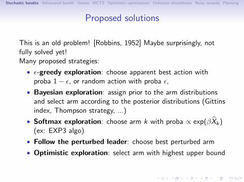
This is an old problem! [Robbins, 1952] Maybe surprisingly, notfully solved yet!Many proposed strategies:

• ϵ-greedy exploration: choose apparent best action withproba 1− ϵ, or random action with proba ϵ,

• Bayesian exploration: assign prior to the arm distributionsand select arm according to the posterior distributions (Gittinsindex, Thompson strategy, ...)

• Softmax exploration: choose arm k with proba ∝ exp(βXk)(ex: EXP3 algo)

• Follow the perturbed leader: choose best perturbed arm

• Optimistic exploration: select arm with highest upper bound

. . . . . .


The UCB algorithm

Upper Confidence Bound algorithm [Auer, Cesa-Bianchi,Fischer, 2002]: at each time n, select the arm k with highestBk,nk ,n value:

Bk,nk ,ndef=

1

nk

nk∑s=1

xk,s︸︷︷︸Xk,nk

+

√3 log(n)

2nk︸︷︷︸cnk ,n

,

with:

• nk is the number of times arm k has been pulled up to time n

• xk,s is the s-th reward received when pulling arm k.

Note that

• Sum of an exploitation term and an exploration term.

• cnk ,n is a confidence interval term, so Bk,nk ,n is a UCB.

. . . . . .


Intuition of the UCB algorithm

Idea:

• ”Optimism in the face of uncertainty” principle

• Select the arm with highest upper bound (on the true value ofthe arm, given what has been observed so far).

• The B-values Bk,s,t are UCBs on µk . Indeed:

P(Xk,s − µk ≥√

3 log(t)

2s) ≤ 1

t3,

P(Xk,s − µk ≤ −√

3 log(t)

2s) ≤ 1

t3

Reminder of Chernoff-Hoeffding inequality:

P(Xk,s − µk ≥ ϵ) ≤ e−2sϵ2

P(Xk,s − µk ≤ −ϵ) ≤ e−2sϵ2

. . . . . .


Regret bound for UCB

Proposition 1.

Each sub-optimal arm k is visited in average, at most:

Enk(n) ≤ 6log n

∆2k

+ 1 +π2

3

times (where ∆kdef= µ∗ − µk > 0).

Thus the expected regret is bounded by:

ERn =∑k

E[nk ]∆k ≤ 6∑

k:∆k>0

log n

∆k+ K (1 +

π2

3).

. . . . . .


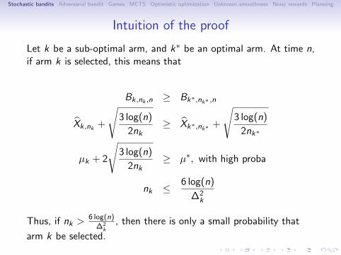
Intuition of the proof

Let k be a sub-optimal arm, and k∗ be an optimal arm. At time n,if arm k is selected, this means that

Bk,nk ,n ≥ Bk∗,nk∗ ,n

Xk,nk +

√3 log(n)

2nk≥ Xk∗,nk∗ +

√3 log(n)

2nk∗

µk + 2

√3 log(n)

2nk≥ µ∗, with high proba

nk ≤ 6 log(n)

∆2k

Thus, if nk > 6 log(n)∆2

k, then there is only a small probability that

arm k be selected.

. . . . . .


Proof of Proposition 1

Write u = 6 log(n)∆2

k+ 1. We have:

nk(n) ≤ u +n∑

t=u+1

1kt = k; nk(t) > u

≤ u +n∑

t=u+1

[ t∑s=u+1

1Xk,s − µk ≥ ct,s+t∑

s=1

1Xk∗,s∗ − µk ≤ −ct,s∗]

Now, taking the expectation of both sides,

E[nk(n)] ≤ u +n∑

t=u+1

[ t∑s=u+1

P(Xk,s − µk ≥ ct,s

)+

t∑s=1

P(Xk∗,s∗ − µk ≤ −ct,s∗

)]≤ u +

n∑t=u+1

[ t∑s=u+1

t−3 +t∑

s=1

t−3]≤ 6 log(n)

∆2k

+ 1 +π2

3

. . . . . .


Variants of UCB

• UCB-V [Audibert et al., 2007] uses empirical variance:

Bk,tdef= µk,t +

√2σk,t

2 log(1.2t)

Tk(t)+

3 log(1.2t)

Tk(t).

Then the expected regret is bounded as:

ERn ≤ 10( ∑

k:∆k>0

σ2k

∆k+ 2

)log(n).

. . . . . .


KL-UCB[Garivier & Cappe, 2011] and [Maillard et al., 2011].For Bernoulli distributions, define the kl-UCB

Bk,tdef= sup

x ∈ [0, 1], kl(µk(t), x) ≤

log t

Tk(t)

Bk,t

kl(µk(t), x)

µk(t)

log tTk(t)

(non-asymptotic version of Sanov’s theorem)

. . . . . .


KL-UCB

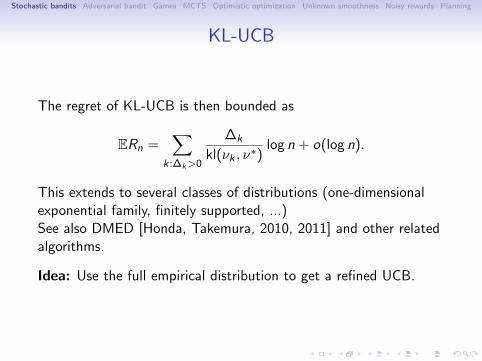
The regret of KL-UCB is then bounded as

ERn =∑

k:∆k>0

∆k

kl(νk , ν∗)log n + o(log n).

This extends to several classes of distributions (one-dimensionalexponential family, finitely supported, ...)See also DMED [Honda, Takemura, 2010, 2011] and other relatedalgorithms.

Idea: Use the full empirical distribution to get a refined UCB.

. . . . . .


Lower bounds

For single-dimensional distributions [Lai, Robbins, 1985]:

lim infn→∞

ERn

log n≥

∑k:∆k>0

∆k

KL(νk , ν∗)

For larger class of distributions D [Burnetas, Katehakis, 1996]:

lim infn→∞

ERn

log n≥

∑k:∆k>0

∆k

Kinf(νk , µ∗),

where

Kinf(ν, µ)def= inf

KL(ν, ν ′) : ν ′ ∈ D and EX∼ν′ [X ] > µ

.

. . . . . .


The adversarial banditThe rewards are no more i.i.d., but arbitrary!At time t, simultaneously

• The adversary assigns a reward xk,t ∈ [0, 1] to each armk ∈ 1, . . . ,K

• The player chooses an arm kt

The player receives the corresponding reward xkt . His goal is tomaximize the sum of rewards.

Can we expect to do almost as good as the best (constant) arm?

Time 1 2 3 4 5 6 7 8 ...

Arm pulled 1 2 1 1 2 1 1 1

Reward arm 1 1 0.7 0.9 1 1 1 0.8 1Reward arm 2 0.9 0 1 0 0.4 0 0.6 0

Reward obtained: 6.1. Arm 1: 7.4, Arm 2: 2.9.Regret w.r.t. best constant strategy: 7.4− 6.1 = 1.3.

. . . . . .


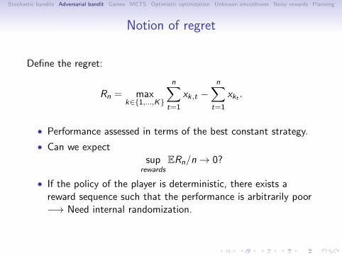
Notion of regret

Define the regret:

Rn = maxk∈1,...,K

n∑t=1

xk,t −n∑

t=1

xkt .

• Performance assessed in terms of the best constant strategy.

• Can we expectsup

rewardsERn/n → 0?

• If the policy of the player is deterministic, there exists areward sequence such that the performance is arbitrarily poor−→ Need internal randomization.

. . . . . .


EXP3 algorithm

EXP3 algorithm (Explore-Exploit using Exponential weights)[Auer et al, 2002]:

• η > 0 and β > 0 are two parameters of the algorithm.

• Initialize w1(k) = 1 for all k = 1, . . . ,K .

• At each round t = 1, . . . , n, player selects arm kt ∼ pt(·),where

pt(k) = (1− β)wt(k)∑Ki=1 wt(i)

+β

K,

withwt(k) = eη

∑t−1s=1 xs(k),

where

xs(k) =xs(k)

ps(k)1ks = k.

. . . . . .


Performance of EXP3

Proposition 2.

Let η ≤ 1 and β = ηK. We have ERn ≤ logKη + (e − 1)ηnK . Thus,

by choosing η =√

logK(e−1)nK , it comes

suprewards

ERn ≤ 2.63√

nK logK .

Properties:

• If all rewards are provided to the learner, with a similaralgorithms we have [Lugosi and Cesa-Bianchi, 2006]

suprewards

ERn = O(√

n logK ).

. . . . . .


Proof of Proposition 2 [part 1]

Write Wt =∑K

k=1 wk(t). Notice that

Eks∼ps [xs(k)] =K∑i=1

ps(i)xs(k)

ps(k)1i = k = xs(k),

and Eks∼ps [xs(ks)] =K∑i=1

ps(i)xs(i)

ps(i)≤ K .

We thus have

Wt+1

Wt=

K∑k=1

wk(t)eηxt(k)

Wt=

K∑k=1

pk(t)− β/K

1− βeηxt(k)

≤K∑

k=1

pk(t)− β/K

1− β(1 + ηxt(k) + (e − 2)η2xt(k)

2),

since ηxt(k) ≤ ηK/β = 1, and ex ≤ 1 + x + (e − 2)x2 for x ≤ 1.

. . . . . .



Thus

Wt+1

Wt≤ 1 +

1

1− β

K∑k=1

pk(t)(ηxt(k) + (e − 2)η2xt(k)2),

logWt+1

Wt≤ 1

1− β

K∑k=1

pk(t)(ηxt(k) + (e − 2)η2xt(k)2),

logWn+1

W1≤ 1

1− β

n∑t=1

K∑k=1

pk(t)(ηxt(k) + (e − 2)η2xt(k)2).

But we also have

logWn+1

W1= log

K∑k=1

eη∑n

t=1 xt(k) − logK ≥ η

n∑t=1

xt(k)− logK ,

for any k = 1, . . . , n.

. . . . . .



Take expectation w.r.t. internal randomization of the algo, thus forall k,

E[(1− β)

n∑t=1

xt(k)−n∑

t=1

K∑i=1

pi (t)xt(i)]

≤ (1− β)logK

η

+ (e − 2)ηE[ n∑

t=1

K∑k=1

pk(t)xt(k)2]

E[ n∑

t=1

xt(k)−n∑

t=1

xt(kt)]

≤ βn +logK

η+ (e − 2)ηnK

E[Rn(k)] ≤ logK

η+ (e − 1)ηnK

. . . . . .


Population of bandits

• Bandit (or regret minimization) algorithms = tool for rapidlyselecting the best action.

• Basic building block for solving more complex problems

• We now consider a population of bandits:

Adversarial bandits Collaborative bandits

. . . . . .


Game between bandits

Consider a 2-players zero-sum repeated game:A and B play actions: 1 or 2 simultaneously, and receive thereward (for A):

A \ B 1 2

1 2 0

2 -1 1(A likes consensus, B likes conflicts)

Now, let A and B be bandit algorithms, aiming at minimizing theirregret, i.e. for player A:

Rn(A)def= max

a∈1,2

n∑t=1

rA(a,Bt)−n∑

t=1

rA(At ,Bt).

What happens?

. . . . . .


Nash equilibrium

Nash equilibrium: (mixed) strategy for both players, such that noplayer has incentive for changing unilaterally his own strategy.

A \ B 1 2

1 2 0

2 -1 1

Here: A plays 1 with probabilitypA = 1/2, B plays 1 with proba-bility pB = 1/4.

1 A

B=1

B=2

2

Ar

. . . . . .


Regret minimization → Nash equilibrium

Define the regret of A:

Rn(A)def= max

a∈1,2

n∑t=1

rA(a,Bt)−n∑

t=1

rA(At ,Bt).

and that of B accordingly.

Proposition 3.

If both players perform a (Hannan) consistent regret-minimizationstrategy (i.e. Rn(A)/n → 0 and Rn(B)/n → 0), then the empiricalfrequencies of chosen actions of both players converge to a Nashequilibrium.

(Remember that EXP3 is consistent!)Note that in general, we have convergence towards correlatedequilibrium [Foster and Vohra, 1997].

. . . . . .


Sketch of proof:Write pnA

def= 1

n

∑nt=1 1At=1 and pnB

def= 1

n

∑nt=1 1Bt=1 and

rA(p, q)def= ErA(A ∼ p,B ∼ q).

Regret-minimization algorithm: Rn(A)/n → 0 means that: ∀ε > 0,for n large enough,

maxa∈1,2

1

n

n∑t=1

rA(a,Bt)−1

n

n∑t=1

rA(At ,Bt) ≤ ε

maxa∈1,2

rA(a, pnB)− rA(p

nA, p

nB) ≤ ε

rA(p, pnB)− rA(p

nA, p

nB) ≤ ε,

for all p ∈ [0, 1]. Now, using Rn(B)/n → 0 we deduce that:

rA(p, pnB)− ε ≤ rA(p

nA, p

nB) ≤ rA(p

nA, q) + ε, ∀p, q ∈ [0, 1]

Thus the empirical frequencies of actions played by both players isarbitrarily close to a Nash strategy.

. . . . . .


Texas Hold’em Poker

• In the 2-players Poker game, theNash equilibrium is interesting(zero-sum game)

• A policy:information set (my cards + board+ pot) → probabilities overdecisions (check, raise, fold)

• Space of policies is huge!

Idea: Approximate the Nash equilibrium by using banditalgorithms assigned to each information set.

• This provides the world best Texas Hold’em Poker programfor 2-player with pot-limit [Zinkevich et al., 2007]

. . . . . .


Monte Carlo Tree Search

MCTS in Crazy-Stone (Remi Coulom, 2005)

Idea: use bandits at each node.

. . . . . .


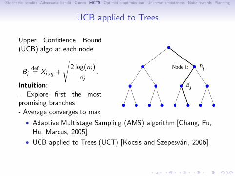
UCB applied to Trees

Upper Confidence Bound(UCB) algo at each node

Bjdef= Xj ,nj +

√2 log(ni )

nj.

Intuition:- Explore first the mostpromising branches- Average converges to max

Node i: Bi

Bj

• Adaptive Multistage Sampling (AMS) algorithm [Chang, Fu,Hu, Marcus, 2005]

• UCB applied to Trees (UCT) [Kocsis and Szepesvari, 2006]

. . . . . .


The MoGo program

[Gelly et al., 2006] + collaborative work with many others.

Features:

• Explore-Exploit with UCT

• Monte-Carlo evaluation

• Asymmetric treeexpansion

• Anytime algo

• Use of features

Among world best programs!

. . . . . .


No finite-time guarantee for UCT

Problem: at each node, the rewards are not i.i.d.Consider the tree:

The left branches seem betterthan right branches, thus are ex-plored for a very long time be-fore the optimal leaf is eventuallyreached.The expected regret is disastrous:

ERn = Ω(exp(exp(. . . exp(︸︷︷︸D times

1) . . . )))+O(log(n)).

See [Coquelin and Munos, 2007]

D−1

D

D−2

D

D−3

D

1

D

10

. . . . . .


Optimism for decision making

Outline:

• Optimization of deterministic Lipschitz functions

• Extension to locally smooth functions,• when the metric is known,• and when it’s not

• Extension to the stochastic case

• Application to planning in MDPs

. . . . . .


Optimization of a deterministic Lipschitz function

Problem: Find online the maximum of f : X → IR, assumed to beLipschitz:

|f (x)− f (y)| ≤ ℓ(x , y).

Protocol:

• For each time step t = 1, 2, . . . , n select a state xt ∈ X

• Observe f (xt)

• Return a state x(n)

Performance assessed in terms of the loss

rn = f ∗ − f (x(n)),

where f ∗ = supx∈X f (x).

. . . . . .


Example in 1d

f(x )t

xt

f

f *

Lipschitz property → the evaluation of f at xt provides a firstupper-bound on f .

. . . . . .


Example in 1d (continued)

New point → refined upper-bound on f .

. . . . . .


Example in 1d (continued)

Question: where should one sample the next point?Answer: select the point with highest upper bound!“Optimism in the face of (partial observation) uncertainty”

. . . . . .


Several issues

1. Lipschitz assumption is too strong

2. Finding the optimum of the upper-bounding function may behard!

3. What if we don’t know the metric ℓ?

4. How to handle noise?

. . . . . .


Local smoothness property

Assumption: f is “locally smooth” around its max. w.r.t. ℓwhere ℓ is a semi-metric (symmetric, and ℓ(x , y) = 0 ⇔ x = y):For all x ∈ X ,

f (x∗)− f (x) ≤ ℓ(x , x∗).

x∗ X

f(x∗) f

f(x∗)− ℓ(x, x∗)

. . . . . .


Local smoothness is enough!

x∗

f(x∗)

f

Optimistic principle only requires:

• a true bound at the maximum

• the bounds gets refined when adding more points

. . . . . .


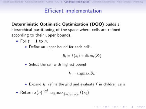
Efficient implementation

Deterministic Optimistic Optimization (DOO) builds ahierarchical partitioning of the space where cells are refinedaccording to their upper bounds.

• For t = 1 to n,• Define an upper bound for each cell:

Bi = f (xi ) + diamℓ(Xi )

• Select the cell with highest bound

It = argmaxi

Bi .

• Expand It : refine the grid and evaluate f in children cells

• Return x(n)def= argmaxxt1≤t≤n

f (xt)

. . . . . .


Near-optimality dimension

Define the near-optimality dimension of f as the smallest d ≥ 0such that ∃C , ∀ϵ, the set of ε-optimal states

Xεdef= x ∈ X , f (x) ≥ f ∗ − ε

can be covered by Cε−d ℓ-balls of radius ε.

. . . . . .


Example 1:

Assume the function is piecewise linear at its maximum:

f (x∗)− f (x) = Θ(||x∗ − x ||).

ε

ε

Using ℓ(x , y) = ∥x − y∥, it takes O(ϵ0) balls of radius ϵ to coverXε. Thus d = 0.

. . . . . .


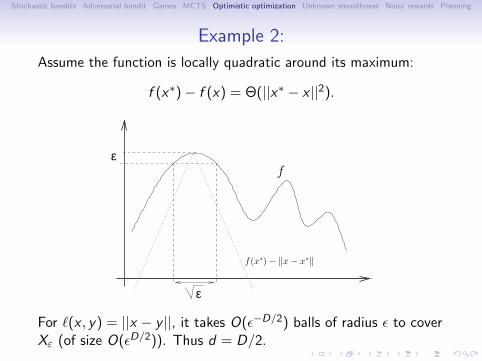
Example 2:

Assume the function is locally quadratic around its maximum:

f (x∗)− f (x) = Θ(||x∗ − x ||2).

ε

εf

f(x∗)− ‖x− x∗‖

For ℓ(x , y) = ||x − y ||, it takes O(ϵ−D/2) balls of radius ϵ to coverXε (of size O(ϵD/2)). Thus d = D/2.

. . . . . .


Example 2:

Assume the function is locally quadratic around its maximum:

f (x∗)− f (x) = Θ(||x∗ − x ||2)

ε

ε

f

f(x∗)− ‖x− x∗‖2

For ℓ(x , y) = ||x − y ||2, it takes O(ϵ0) ℓ-balls of radius ϵ to coverXε. Thus d = 0.

. . . . . .


Example 3:

Assume the function has a square-root behavior around itsmaximum:

f (x∗)− f (x) = Θ(||x∗ − x ||1/2)

ε

ε

f

f(x∗)− ‖x− x∗‖1/2

For ℓ(x , y) = ∥x − y∥1/2 we have d = 0.

. . . . . .


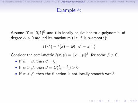
Example 4:

Assume X = [0, 1]D and f is locally equivalent to a polynomial ofdegree α > 0 around its maximum (i.e. f is α-smooth):

f (x∗)− f (x) = Θ(||x∗ − x ||α)

Consider the semi-metric ℓ(x , y) = ∥x − y∥β, for some β > 0.

• If α = β, then d = 0.

• If α > β, then d = D( 1β − 1α) > 0.

• If α < β, then the function is not locally smooth wrt ℓ.

. . . . . .


Analysis of DOO (deterministic case)

Assume that the ℓ-diameters of the nodes of depth h decreaseexponentially fast with h (i.e., diam(h) = cγh, for some c > 0 andγ < 1).This is true for example when X = [0, 1]D and ℓ(x , y) = ∥x − y∥βfor some β > 0.

Theorem 1.The loss of DOO is

rn =

(

C1−γd

)1/dn−1/d for d > 0,

cγn/C−1 for d = 0.

(Remember that rndef= f (x∗)− f (x(n))).

. . . . . .


About the local smoothness assumption

Assume f satisfies f (x∗)− f (x) = Θ(||x∗ − x ||α).

Use DOO with the semi-metric ℓ(x , y) = ∥x − y∥β:• If α = β, then d = 0: the true “local smoothness” of thefunction is known, and exponential rate is achieved.

• If α > β, then d = D( 1β − 1α) > 0: we under-estimate the

smoothness, which causes more exploration than needed.

• If α < β: We over-estimate the true smoothness and DOOmay fail to find the global optimum.

The performance of DOO heavilly relies on our knowledge of thetrue local smoothness.

. . . . . .


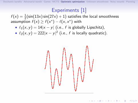
Experiments [1]f (x) = 1

2(sin(13x) sin(27x) + 1) satisfies the local smoothnessassumption f (x) ≥ f (x∗)− ℓ(x , x∗) with

• ℓ1(x , y) = 14|x − y | (i.e., f is globally Lipschitz),

• ℓ2(x , y) = 222|x − y |2 (i.e., f is locally quadratic).

. . . . . .


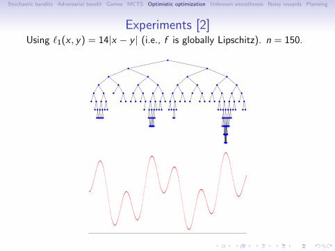
Experiments [2]Using ℓ1(x , y) = 14|x − y | (i.e., f is globally Lipschitz). n = 150.

The trees Tn built by DOO after n = 150 evaluations.

. . . . . .


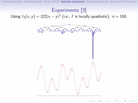
Experiments [3]Using ℓ2(x , y) = 222|x − y |2 (i.e., f is locally quadratic). n = 150.

The trees Tn built by DOO after n = 150 evaluations.

. . . . . .


Experiments [4]

n uniform grid DOO with ℓ1 (d = 1/2) DOO with ℓ2 (d = 0)

50 1.25× 10−2 2.53× 10−5 1.20× 10−2

100 8.31× 10−3 2.53× 10−5 1.67× 10−7

150 9.72× 10−3 4.93× 10−6 4.44× 10−16

Loss rn for different values of n for a uniform grid and DOO withthe two semi-metric ℓ1 and ℓ2.

. . . . . .


What if the smoothness is unknown?

Previous algorithms heavily rely on the knowledge or the localsmoothness of the function (i.e. knowledge of the best metric).

Question: When the smoothness is unknown, is it possible toimplement the optimistic principle for function optimization?

. . . . . .


DIRECT algorithm [Jones et al., 1993]

Assumes f is Lipschitz but the Lipschitz constant L is unknown.

The DIRECT algorithm expands simultaneously all nodes that maypotentially contain the maximum for some value of L.

. . . . . .


Illustration of DIRECTThe sin function and its upper bound for L = 2.

. . . . . .


Illustration of DIRECTThe sin function and its upper bound for L = 1/2.

. . . . . .


Simultaneous Optimistic Optimization (SOO)

Extends DIRECT to any semi-metric ℓ and for any function locallysmooth w.r.t. ℓ.

[Munos, 2011]

• Expand several leaves simultaneously

• SOO expands at most one leaf per depth

• SOO expands a leaf only if its value is larger that the value ofall leaves of same or lower depths.

• At round t, SOO does not expand leaves with depth largerthan hmax(t)

. . . . . .


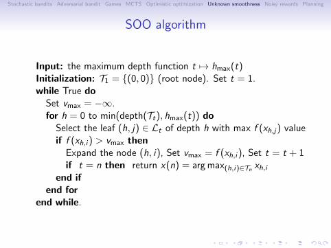
SOO algorithm

Input: the maximum depth function t 7→ hmax(t)Initialization: T1 = (0, 0) (root node). Set t = 1.while True doSet vmax = −∞.for h = 0 to min(depth(Tt), hmax(t)) do

Select the leaf (h, j) ∈ Lt of depth h with max f (xh,j) valueif f (xh,i ) > vmax then

Expand the node (h, i), Set vmax = f (xh,i ), Set t = t + 1if t = n then return x(n) = argmax(h,i)∈Tn xh,i

end ifend for

end while.

. . . . . .


. . . . . .


. . . . . .


. . . . . .


. . . . . .


. . . . . .


. . . . . .


. . . . . .


. . . . . .


. . . . . .


. . . . . .


. . . . . .


. . . . . .


Performance of SOO

Theorem 2.For any semi-metric ℓ such that

• f is locally smooth w.r.t. ℓ

• The ℓ-diameter of cells of depth h is cγh

• The near-optimality dimension of f w.r.t. ℓ is d = 0,

by choosing hmax(n) =√n, the expected loss of SOO is

rn ≤ cγ√n/C−1

In the case d > 0 a similar statement holds with Ern = O(n−1/d).

. . . . . .


Performance of SOO

Remarks:

• Since the algorithm does not depend on ℓ, the analysis holdsfor the best possible choice of the semi-metric ℓ satisfying theassumptions.

• SOO does almost as well as DOO optimally fitted (thus“adapts” to the unknown local smoothness of f ).

. . . . . .


Numerical experiments

Again for the function f (x) = (sin(13x) sin(27x) + 1)/2 we have:

n SOO uniform grid DOO with ℓ1 DOO with ℓ250 3.56× 10−4 1.25× 10−2 2.53× 10−5 1.20× 10−2

100 5.90× 10−7 8.31× 10−3 2.53× 10−5 1.67× 10−7

150 1.92× 10−10 9.72× 10−3 4.93× 10−6 4.44× 10−16

. . . . . .


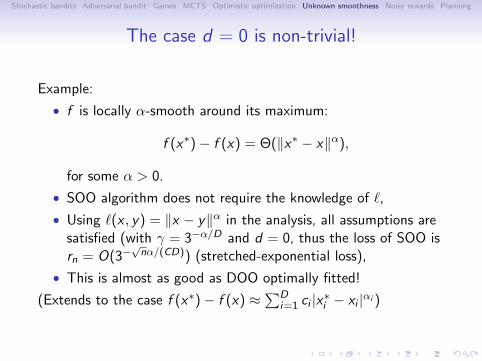
The case d = 0 is non-trivial!

Example:

• f is locally α-smooth around its maximum:

f (x∗)− f (x) = Θ(∥x∗ − x∥α),

for some α > 0.

• SOO algorithm does not require the knowledge of ℓ,

• Using ℓ(x , y) = ∥x − y∥α in the analysis, all assumptions aresatisfied (with γ = 3−α/D and d = 0, thus the loss of SOO isrn = O(3−

√nα/(CD)) (stretched-exponential loss),

• This is almost as good as DOO optimally fitted!

(Extends to the case f (x∗)− f (x) ≈∑D

i=1 ci |x∗i − xi |αi )

. . . . . .


The case d = 0

More generally, any function whose upper- and lower envelopesaround x∗ have the same shape: ∃c > 0 and η > 0, such that

min(η, cℓ(x , x∗)) ≤ f (x∗)− f (x) ≤ ℓ(x , x∗), for all x ∈ X .

has a near-optimality d = 0 (w.r.t. the metric ℓ).

x∗

f(x∗) f(x∗)− cℓ(x, x∗)

f(x∗)− ℓ(x, x∗)

f(x∗)− η

. . . . . .


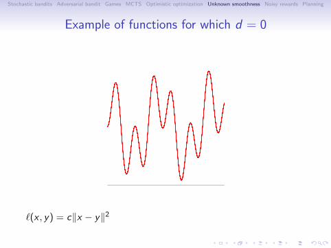
Example of functions for which d = 0

ℓ(x , y) = c∥x − y∥2

. . . . . .


Example of functions with d = 0

ℓ(x , y) = c∥x − y∥1/2

. . . . . .


d = 0?

ℓ(x , y) = c∥x − y∥1/2

. . . . . .


d > 0

f (x) = 1−√x + (−x2 +

√x) ∗ (sin(1/x2) + 1)/2

The lower-envelope is of order 1/2 whereas the upper one is oforder 2. We deduce that d = 3/2 and rn = O(n−2/3).

. . . . . .


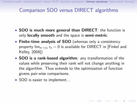
Comparison SOO versus DIRECT algorithms

• SOO is much more general than DIRECT: the function isonly locally smooth and the space is semi-metric.

• Finite-time analysis of SOO (whereas only a consistencyproperty limn→∞ rn = 0 is available for DIRECT in [Finkel andKelley, 2004])

• SOO is a rank-based algorithm: any transformation of thevalues while preserving their rank will not change anything inthe algorithm. Thus extends to the optimization of functiongivens pair-wise comparisons.

• SOO is easier to implement...

. . . . . .


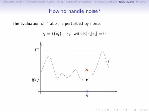
How to handle noise?

The evaluation of f at xt is perturbed by noise:

rt = f (xt) + ϵt , with E[ϵt |xt ] = 0.

f(x )t

xt

f

f *

. . . . . .


Where should one sample next?

x

How to define a high probability upper bound at any state x?

. . . . . .


UCB in a given cell

xt

f(xt)

rt

x

For a fixed domain Xi ∋ x containing Ti points xt ∈ Xi , we have

that∑Ti

t=1 rt − f (xt) is a Martingale. Thus by Azuma’s inequality,with 1/n-confidence,

1

Ti

Ti∑t=1

rt +

√log n

2Ti≥ 1

Ti

Ti∑t=1

f (xt).

. . . . . .


Stochastic SOO (StoSOO)

A simple way to extends SOO to the case of stochastic rewards isthe following:

• Select a cell i (and sample f at xi ) according to SOO basedon the values

µi ,t + c

√log n

Ti (t),

• Expand the cell Xi only if Ti (t) ≥ k, where k is a parameter.

Remark: This really looks like UCT, except that

• several cells are selected at each round,

• a cell is refined only when we received k samples.

. . . . . .


Performance of StoSOO

Theorem 3 (Valko et al., 2013).

For any semi-metric ℓ such that

• f is locally smooth w.r.t. ℓ

• The ℓ-diameters of the cells decrease exponentially fast withtheir depth,

• The near-optimality dimension of f w.r.t. ℓ is d = 0,

by choosing k = n(log n)3

, hmax(n) = (log n)3/2, the expected loss of

StoSOO is

Ern = O((log n)2√

n

).

. . . . . .


Online planning in a MDP

Setting:

• Assume we have a model of the MDP.

• The state space is large: no way to approximate the valuefunction

• Search for the best policy given an initial state, using a finitenumerical budget (number of calls to the model)

Protocol:

• From current state sk , perform planning using n calls to themodel and recommend action a(n),

• Play a(n), observe next state sk+1, and repeat

Loss: rndef= max

a∈AQ∗(sk , a)− Q∗(sk , a(n)).

. . . . . .


Deterministic transitions and rewards

(infinite time horizon and discounted setting)

• A policy x is an infinite path

• Value f (x) =∑

s≥0 γsrs(x), where

the rewards are in [0, 1]

• Metric: ℓ(x , y) = γh(x,y)

1−γ

• Prop: f (x) is Lipschitz w.r.t. ℓ

• → Use optimistic search

Initial state

xy

h(x, y) = 2

. . . . . .


OPD algorithm

Optimistic Planning in Deterministic systems:

• Define the B-values:

Bidef=

d(i)∑s=0

γsrs +γd(i)+1

1− γ

• We have Bi ≥ maxx∋i f (x)

• For each round t = 1 to n,expand the node withhighest B-value

• Observe reward, updateB-values

Optimal path

Expandednodes

Node i

Recommend the first action a(n) of the best policy.

. . . . . .


Performance of OPD

Define β such that P(Random path is ϵ-optimal) = O(ϵβ).

Define κdef= Kγβ ∈ [1,K ]. Then κ is the branching factor of the

set of near-optimal sequences:

I =sequences of length h such that

h∑s=0

γs rs ≥ V ∗ − γh+1

1− γ

.

Property: κ relates to the near-opt. dimension d = log κlog 1/γ (the set

of ϵ-optimal paths is covered by O(ϵ−d) ℓ-balls of radius ϵ)

Loss of OPD [Hren and Munos, 2008]:

rn = O(n−1d ) = O

(n−

log 1/γlog κ

).

Performance depends on the quantity of near-optimal policies

. . . . . .


κ-minimax lower bounds

Let Mκ the set of problems with coefficient κ.Upper-bound of OPD uniformly over Mκ

supM∈Mκ

rn(AOPD ,M) = O

(n−

log 1/γlog κ

).

We can prove that we have a κ-minimax lower-bound:

supA

infM∈Mκ

rn(A,M) ≥ Ω

(n−

log 1/γlog κ

).

Sketch of proof:OPD only expands nodes in I . Reciproquely, I is the set of nodesthat need to be expanded in order to find the optimal path.

. . . . . .


Extension to stochastic rewards

Dynamics are still deterministic thus the space of policies is stillthe set of sequences of actions.

Stochastic rewards:

• Reward along a path x :∑s≥0γ

sYs ,

where Ys ∼ νs(x) where νs(x) isthe reward distribution (∈ [0, 1])after s actions along path x .

• Write rs(x) = EX∼νs(x)[X ] andf (x) =

∑s≥0 γ

srs(x)x

Y2 ∼ ν2(x)

Y1 ∼ ν1(x)

Y0 ∼ ν0(x)

Then f (x) is Lipschitz w.r.t. ℓ(x , y) = γh(x,y)

1−γ and one can think ofapplying HOO.

. . . . . .


Using HOO for planning

Apply HOO to the search space X :

• Assign a B-value to each finite sequence

• At each round t, select a finite sequence xt maximizing theB-value.

• Observe sample reward∑

s≥0 γsYs(xt) of the path xt and use

it to update the B-values.

• The loss isO(n−

1d+2 ).

Problem: HOO does not make full use of the tree structure:It uses the sample reward of the whole path x but not theindividual reward samples Ys(x) collected along the path x .

. . . . . .


Optimistic sampling using the tree structure

Open Loop Optimistic Planning (OLOP) [Bubeck, Munos,2010]:

• At round t, play path xt (up to depth h = 12

log nlog 1/γ )

• Observe sample rewards Ys(xt) of each node along the path xt

• Compute empirical rewards µt(x1:s) for each node x1:s ofdepth s ≤ h

• Define bound for each path x :

Bt(x) = min1≤j≤h

[ j∑s=0

γs(µt(x1:s) +

√2 log n

Tx1:s (t)

)+

γj+1

1− γ

]• Select path xt+1 = argmaxx Bt(x)

This algorithm fully uses the tree structure of the rewards.

. . . . . .


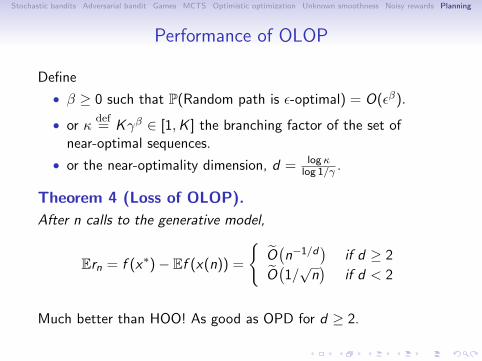
Performance of OLOP

Define

• β ≥ 0 such that P(Random path is ϵ-optimal) = O(ϵβ).

• or κdef= Kγβ ∈ [1,K ] the branching factor of the set of

near-optimal sequences.

• or the near-optimality dimension, d = log κlog 1/γ .

Theorem 4 (Loss of OLOP).

After n calls to the generative model,

Ern = f (x∗)− Ef (x(n)) =

O(n−1/d

)if d ≥ 2

O(1/

√n)

if d < 2

Much better than HOO! As good as OPD for d ≥ 2.

. . . . . .


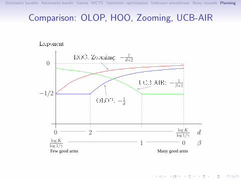
Comparison: OLOP, HOO, Zooming, UCB-AIR

Many good armsFew good arms

logKlog 1/γ

logKlog 1/γ

d

β

0 2

1 0

Exponent

0HOO, Zooming:

OLOP:

UCB-AIR:

−

1d+2

−

1d

−

1β+1

−1/2

. . . . . .


Optimistic Planning in MDPs

Stochastic transitions, but assume that the number of next statesis finite.

Here a policy is no more a sequence of actions

OP-MDP [Busoniu and Munos, 2012]:

• The root = current state.

• For t = 1 to n:• Compute the B-value of all nodes of the current sub-tree• Compute the optimistic policy• Select a leaf of the optimistic sub-tree and expand it

(generates transitions to next states using the model)

• Return first action of the best policy

. . . . . .


Illustration of OP-MDP

B-values: upper-bounds on the optimal value function V ∗(s):

B(s) =1

1− γfor leaves

B(s) = maxa

∑s′

p(s ′|s, a)[r(s, a, s ′) + γB(s ′)

]Compute the optimistic policy π+.

. . . . . .


Optimistic Planning in MDPs

Expand leaf in π+ with largest contribution: argmaxs∈L P(s)γd(s)

1−γ ,

where P(s) is the probability to reach s when following π+.

. . . . . .


Performance analysis of OP-MDP

Define Xϵ the set of states

• whose “contribution” is at least ϵ

• and that belong to an ϵ-optimal policy

Near-optimality planning dimension: Define the measure ofcomplexity of planning in the MDP as the smallest d ≥ 0 suchthat |Xϵ| = O(ϵ−d).

Theorem 5.The performance of OP-MDP is rn = O(n−1/d).

The performance depends on the quantity of states thatcontribute significantly to near-optimal policies

. . . . . .


Illustration of the performance

Reminder: rn = O(n−1/d).

Uniform rewards and probabilities d = logK+logNlog 1/γ (uniform

planning)

Structured rewards, uniform probabilities d = logNlog 1/γ (uniform

planning for a single policy)

Uniform rewards, concentrated probabilities d → logKlog 1/γ

(planning in deterministic systems)

Structured rewards, concentrated probabilities d → 0(exponential rate)

Remarks: d is small when

• Structured rewards

• Heterogeneous transition probabilities

. . . . . .


Towards d-minimax lower bounds

Let Md the set of MDPs with near-optimality planning dim. dUpper-bound of OP-MDP uniformly over Mβ

supM∈Md

rn(AOP−MDP ,M) ≤ O(n−1/d).

We conjecture that we have a d-minimax lower-bound:

supA

infM∈Md

Ern(A,M) ≥ Ω(n−1/d).

. . . . . .


Conclusions on optimistic planning

• Perform optimistic search in policy space.

• In deterministic dynamics, deterministic rewards, can be seenas a direct application of optimistic optimization

• In stochastic rewards, the structure of the reward function canhelp estimation of paths given samples from other paths

• In MDPs the near-optimality planning dimension is a newmeasure of the quantity of states that need to be expanded(the set of states that significantly contribute to near-optimalpolicies)

• Fast rates when the MDP has structured rewards andheterogeneous transition probabilities.

• Applications to Bayesian Reinforcement learning and planningin POMDPs.

. . . . . .


Conclusions

The “optimism in the face of uncertainty” principle:

• applies in a large class of decision making problems instochastic and deterministic environments (in unstructuredand structured problems)

• provides an efficient exploration of the search space byexploring the most promising areas first

• provides a natural transition from global to local search

• Performance depends on the “smoothness” of the functionaround the maximum w.r.t. some metric,

• a measure of the quantity of near-optimal solutions,• and our knowledge or not of this metric.

. . . . . .


About optimism

Optimists and pessimists inhabit different worlds, reacting to thesame circumstances in completely different ways.

Learning to Hope, Daisaku Ikeda.

Habits of thinking need not be forever. One of the most significantfindings in psychology in the last twenty years is that individualscan choose the way they think.

Learned Optimism, Martin Seligman.

Humans do not hold a positivity bias on account of having readtoo many self-help books. Rather, optimism may be so essential toour survival that it is hardwired into our most complex organ, thebrain.

The Optimism Bias:A Tour of the Irrationally Positive Brain, Tali Sharot.

. . . . . .


Thanks !!!

See the review paper

From bandits to Monte-Carlo Tree Search: Theoptimistic principle applied to optimization and planning.

are available from my web page:

http://chercheurs.lille.inria.fr/∼munos/

Documents

Introduction to Reinforcement Learning and multi …chercheurs.lille.inria.fr/~munos/talks/2013/SS_Netadis2013/part3.pdfStochastic bandits Adversarial bandit Games MCTS Optimistic