Deep Learning for Computer VisionSpring 2019

http://vllab.ee.ntu.edu.tw/dlcv.html (primary)

https://ceiba.ntu.edu.tw/1072CommE5052 (grade, etc.)

FB: DLCV Spring 2019

Yu-Chiang Frank Wang 王鈺強, Associate Professor

Dept. Electrical Engineering, National Taiwan University

2019/04/10

What’s to Be Covered Today…

• Image Segmentation• Visualization of NN• Adversarial Attack for NN

Many slides from Fei-Fei Li, Yaser Sheikh, Simon Lucey, Kaiming He, Joseph Lim, and J.-B. Huang 2

Image Segmentation

• Goal: Group pixels into meaningful or perceptually similar regions

3

Segmentation for Object Proposal

“Selective Search” [Sande, Uijlings et al. ICCV 2011, IJCV 2013]

[Endres Hoiem ECCV 2010, IJCV 2014]4

Segmentation via Clustering

• K-means clustering• Mean-shift*

• Find modes of the following non-parametric density

*D. Comaniciu and P. Meer, Mean Shift: A Robust Approach toward Feature Space Analysis, IEEE PAMI 2002. 5

Superpixels

• A simpler task of image segmentation• Divide an image into a large number of regions,

such that each region lies within object boundaries.

• Examples• Watershed• Felzenszwalb and Huttenlocher graph-based• Turbopixels• SLIC

6

Multiple Segmentations

• Don’t commit to one partitioning• Hierarchical segmentation

• Occlusion boundaries hierarchy:Hoiem et al. IJCV 2011 (uses trained classifier to merge)

• Pb+watershed hierarchy: Arbeleaz et al. CVPR 2009• Selective search: FH + agglomerative clustering • Superpixel hierarchy

• Vary segmentation parameters• E.g., multiple graph-based segmentations or mean-shift segmentations

• Region proposals• Propose seed superpixel, try to segment out object that contains it

(Endres Hoiem ECCV 2010, Carreira Sminchisescu CVPR 2010)

7

More Tasks in Segmentation

• Cosegmentation• Segmenting common objects from multiple images

• Instance Segmentation• Assign each pixel an object instance

8

More Tasks in Segmentation

• Semantic Segmentation• Assign a class label to each pixel in the input image• Don’t differentiate instances, only care about pixels

9

Semantic Segmentation

• Sliding Window

10

Semantic Segmentation

• Fully Convolutional Nets

11

Semantic Segmentation

• Fully Convolutional Nets (cont’d)

12

In-Network Upsampling

• Unpooling

13

In-Network Upsampling

• Max Unpooling

14

In-Network Upsampling

• Learnable Upsampling: Transpose Convolution

15

In-Network Upsampling

• Learnable Upsampling: Transpose Convolution

16

In-Network Upsampling

• Transpose Convolution

17

In-Network Upsampling

• Transpose Convolution• 1D example

18

In-Network Upsampling

• Transpose Convolution• Example as matrix multiplication

19

In-Network Upsampling

• Transpose Convolution• Example as matrix multiplication

20

Fully Convolutional Networks (FCN)

• Remarks• All layers are convolutional.• End-to-end training.

21

Fully Convolutional Networks (FCN)

• More details• Adapt existing classification network to fully convolutional forms• Remove flatten layer and replace fully connected layers with conv layers• Use transpose convolution to upsample pixel-wise classification results

22

Fully Convolutional Networks (FCN)

23

Fully Convolutional Networks (FCN)

• Example• VGG16-FCN32s• Loss: pixel-wise cross-entropyi.e., compute cross-entropy between each pixel and its label, and average over all of them

VGG16 (Pretrained)

Input shape: 256 x 256

Coarse prediction shape: 8 x 8

Upsample 32x (transpose conv)

Pixel-wise prediction shape: 256 x 256

24

SegNet

“SegNet: A Deep Convolutional Encoder-Decoder Architecture for Image Segmentation” [link]

• Efficient architecture (memory + computation time)• Upsampling reusing max-unpooling indices• Reasonable results without performance boosting addition• Compaable to FCN

25

U-Net

U-Net: Convolutional Networks for Biomedical Image Segmentation [link]

26

What’s to Be Covered Today…

• Image Segmentation• Visualization of NN

• t-SNE• Visualization of Feature Maps

• Adversarial Attack for NN

Many slides from Fei-Fei Li, Yaser Sheikh, Simon Lucey, Kaiming He, Joseph Lim, and J.-B. Huang 27

What’s to Be Covered Today…

• Visualization of NNs• t-SNE• Visualization of Feature Maps• Neural Style Transfer

• Understanding NNs• Image Translation• Feature Disentanglement

Many slides from Fei-Fei Li, Yaser Sheikh, Simon Lucey, Kaiming He, Samja Fidler, Joseph Lim, Mathew Zeiler and J.-B. Huang 28

Recall That…

• If linear DR is not sufficient, and non-linear DR is of interest…• lsomap, locally linear embedding (LLE), etc.

• t-distributed stochastic neighbor embedding (t-SNE) (by G. Hinton & L. van der Maaten)

29

Dimension Reduction via Local Embedding

• PCA• Finds a global structure in low-dim space preserving data distribution• Suffer from outlier and local inconsistency

• t-SNE• Preserve local structure in the derived low-dim space• However, unlike PCA, cannot easily to embed new data points

30

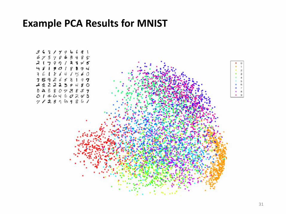
Example PCA Results for MNIST

31

Example t-SNE Results for MNIST

32

Stochastic Neighbor Embedding (SNE)

• Ideas• Encode high-dim neighborhood info as distribution• Intuition:

• encounter a close data point = high probability• Find projected low-dim data with similar neighborhood distributions• How to measure the similarity between distributions?

• KL divergence?

33

Stochastic Neighbor Embedding (SNE) (cont’d)

• Neighborhood Distributions• Consider the neighborhood around an input instance xi in d-dim space• Assume that we have a Gaussian distribution centered at xi

• The probability that xi chooses some other points xj as its neighbor is in proportion with the density/distribution under this Gaussian

• Probability Pij• The i → j probability is the probability that xi chooses xj as its neighbor

• The parameter σ sets the size of the neighborhood.• We have σi differ for each data point.

• Very low σi : ~nearest neighbor• Very large σi : ~uniform weights

34

Stochastic Neighbor Embedding (SNE) (cont’d)

• Perplexity• It is the main parameter.

The higher perplexity, the more the number of neighbors. • For each distribution Pj|i (with σi), we define the perplexity as

• If P is uniform over k elements, perplexity is k.• Low perplexity: small σ2

• High perplexity: larger σ2

• Define the desired perplexity (typically 5~50), and set σi accordingly• Different perplexity captures data distributions in different scales

35

Stochastic Neighbor Embedding (SNE) (cont’d)

• Example Results with Different Perplexities

https://distill.pub/2016/misread-tsne 36

Stochastic Neighbor Embedding (SNE) (cont’d)

• Objective for SNE

37

Stochastic Neighbor Embedding (SNE) (cont’d)

• Algorithm

• Crowding Problem• More room for neighboring data in high-dim space, but not in low-dim space.

In other words, might not have enough room to accommodate all neighbors.• Solution: t-SNE

Change Gaussian in Q to a heavy tailed distribution. If Q changes slower for neighboring data, we have more room to place points accordingly.

38

t-Distributed Stochastic Neighbor Embedding (t-SNE)

• t-SNE

39

t-Distributed Stochastic Neighbor Embedding (t-SNE)

• Remarks• Powerful tool for data visualization• Help understand black-box algorithms like CNN • Alleviate crowding problem• Great resources/tools available

e.g., https://distill.pub/2016/misread-tsne

40

What’s to Be Covered Today…

• Image Segmentation• Visualization of NN

• t-SNE• Visualization of Feature Maps• Neural Style Transfer

• Adversarial Attack for NN

Many slides from Fei-Fei Li, Yaser Sheikh, Simon Lucey, Kaiming He, Joseph Lim, J.-B. Huang, & V. Chen 41

Visualizing CNN

42http://vision03.csail.mit.edu/cnn_art/data/single_layer.png

Activation maximization

43

Activation maximization

• 𝜃𝜃: model parameters

• ℎ𝑖𝑖𝑖𝑖: the activation of a given unit 𝑖𝑖 from a given layer 𝑖𝑖 in the network

• 𝑥𝑥: input sample

• For a fix model 𝜃𝜃, performing gradient ascent in the input space• Hyperparameters: learning rate / stopping criterion

44

• Magnifying the filter response!

Gradient Ascent

45

• Magnifying the filter response!

Gradient Ascent

46

Different Layers of Visualization

47

• Reference:• Visualizing Higher-Layer Features of a Deep Network

Dumitru Erhan, Yoshua Bengio, Aaron C. Courville, Pascal Vincent.Technical Report, Univeristé de Montréal, 2009

• https://distill.pub/2017/feature-visualization/

Visualizing CNN

48

Visualization and Understanding Conv Nets [ECCV’14]

• Remarks• By Matthew Zeiler & Rob Fergus @ NYU• Extension of their CVPR’10 work of Deconvolution Networks• Visualization of conv net over layers• Feature invariance• Experiments on image occlusion

49

Deconvolutional Networks

• Remarks• Provides way to map activations at higher layers back to the input• Same operations as Convnet, but in reverse

• Unpool feature maps• Convolve unpooled maps

with filters copied from Convnet• Used here purely as probe

• Originally proposed asunsupervised learning method

• No inference/learning

50

Reversible Max Pooling

• Illustration

51

Visualization of Higher Layers

• Architecture• 8-layer ConvNet model

52

Visualization of Higher Layers

• Remarks• Use ImageNet 2012 validation set• Push each image through network

53

Layer 1: Top-9 Patches for Each Filter

54

Layer 2: Top-9 Patches for Each Filter

55

Layer 3: Top-9 Patches for Each Filter

56

57

58

59

60

Evolution of Features During Training

61

Evolution of Features During Training

62

Occlusion Experiments

• Motivation• To determine whether the model is truly identifying the location of

the object in the image, or just using the surrounding context.• Mask parts of the input image with a gray square.• Monitor the outputs

63

Occlusion Experiments

• Example

64

Occlusion Experiments

• Example

65

Occlusion Experiments

• Example

66

Occlusion Experiments

• Example

67

What’s to Be Covered Today…

• Image Segmentation• Visualization of NN

• t-SNE• Visualization of Feature Maps• Neural Style Transfer

• Adversarial Attack for NN

Many slides from Fei-Fei Li, Yaser Sheikh, Simon Lucey, Kaiming He, Joseph Lim, and J.-B. Huang 68

Breaking NNs with Adversarial Attacks • Adversarial attack

(Top) Explaining and Harnessing Adversarial Examples, Goodfellow et al, ICLR 2015.(Bottom) Robust Physical-World Attacks on Deep Learning Visual Classification 69

Intriguing properties of neural networks

Christian Szegedy, Wojciech Zaremba, Ilya Sutskever, Joan Bruna, Dumitru Erhan, Ian Goodfellow, Rob Fergus

ICLR 2014

Intriguing Properties of Neural Networks

• Term “adversarial examples”• Add perturbations on inputs to maximize the prediction error

• Adversarial goal: misclassification / target misclassification• Adversarial capability: architecture & training data

71

Adversarial examples

• Left: correctly predicted samples• Center: difference between correct and adversarial samples

• Right: adversarial samples (all images are predicted to be an “ostrich”)

72

• Odd columns: original images• Even columns: perturbed images

Adversarial examplesTesting acc: 0%

Distorted by Gaussian noiseTesting acc: 51%

73

Adversarial examples

How to formulate the problem?

• 𝑓𝑓: classifier• 𝑥𝑥: input image• 𝑙𝑙: target label

• 𝑟𝑟: perturbation• Minimize 𝑟𝑟 2 subject to:

• 𝑓𝑓 𝑥𝑥 + 𝑟𝑟 = 𝑙𝑙• 𝑥𝑥 + 𝑟𝑟 ∈ [0, 1]𝑚𝑚

• Approximated by using a box-constrained L-BFGS

74

Evaluation

• Different models on MNIST

75

76

Cross model generalization

• How “bad” such attacks can generalize across models?

Cross training set generalization

• Different training sets on MNIST• P1, P2 with 30,000 images each

77

78

Cross training set generalization

Categories of Adversarial Attacks

• From easy to hard:• Confidence reduction: reduce the output confidence• Misclassification: alter output to any class different from original class• Targeted misclassification:

produce inputs that force the output classification to be a specific class• Source/target misclassify:

force specific input to be classified as specific target class

Papernot et al. (2015). The Limitations of Deep Learning in Adversarial Settings. 1st IEEE European Symposium on Security & Privacy, IEEE 2016 79

• From easy to hard:• Architecture & training data• Architecture• Training data• Oracle: can obtain output classification from supplied input• Samples: pairs of input and output

Papernot et al. (2015). The Limitations of Deep Learning in Adversarial Settings. 1st IEEE European Symposium on Security & Privacy, IEEE 2016 80

Settings of Adversarial Attacks

Adversarial attack in reality

• Adversarial glasses

https://www.cs.cmu.edu/~sbhagava/papers/face-rec-ccs16.pdf81

Adversarial attack in reality

• Adversarial patch

https://arxiv.org/abs/1712.09665

82

Adversarial Defense

Adversarial defense

• Proactive defense• Add perturbation on input images

to make the model become more robust• Train the model on adversarial examples (data augmentation)

• Reactive defense• Eliminate or alleviate the noise in input images

• Filtering• Autoencoder, VAE

https://arxiv.org/pdf/1712.07107.pdfhttp://speech.ee.ntu.edu.tw/~tlkagk/courses/ML_2019/Lecture/Attack%20(v8).pdf

84

Next Week…

• HW #2 due (now 3+2 free late days) • Guest lecture on deep generative models

by Prof. Wei-Chen Chiu from NCTU

85