Introduction to Nanoscale Thermal Conduction · PDF file0 Introduction to Nanoscale Thermal Conduction Patrick E. Hopkins1,2 and John C. Duda2 1Sandia National Laboratories, Albuquerque,

0

Introduction to Nanoscale Thermal Conduction

Patrick E. Hopkins1,2 and John C. Duda2

1Sandia National Laboratories, Albuquerque, New Mexico2University of Virginia, Charlottesville, Virginia

United States of America

1. Introduction

Thermal conduction in solids is governed by the well-established, phenomenological FourierLaw, which in one-dimension is expressed as

Q = −κ∂T

∂z, (1)

where the thermal flux, Q, is related to the change in temperature, T, along the directionof thermal propagation, z, through the thermal conductivity, κ. The thermal conductivity is atemperature dependent material property that is unique to any given material. Figure 1 showsthe measured thermal conductivity of two metals - Au and Pt - and two semiconductors - Siand Ge (Ho et al., 1972). In these bulk materials, the thermal conductivities span three ordersof magnitude over the temperature range from 1 - 1,000 K. Temperature trends in the thermalconductivities are similar depending on the type of material, i.e., Si and Ge show similarthermal conductivity trends with temperature as do Au and Pt. These similarities arise due tothe different thermal energy carriers in the different classes of materials.In metals, heat is primarily carried by electrons, whereas in semiconductors, heat movesvia atomic vibrations of the crystalline lattice. The macroscopic average of these carriers’scattering events, which is related to the thermal conductivity of the material, gives rise tothe spatial temperature gradient in Eq. 1. This temperature gradient is established from theenergy carriers traversing a certain distance, the mean free path, before scattering and losingtheir thermal energy. In bulk systems, this mean free path is related to the intrinsic propertiesof the materials. However, in material systems with engineered length scales on the orderof the mean free path, additional scattering events arise due to energy carrier scatteringwith interfaces, inclusions, grain boundaries, etc. These scattering events can substantiallychange the thermal conductivity of nanostructured systems as compared to that of the bulkconstituents (Cahill et al., 2003). In fact, in any given material in which the physical size isless than the mean free path, the carrier scattering events will only occur at the boundaries ofthe material. Therefore, there will be no temperature gradient established in the material andEq. 1 will no longer be valid.Typical carrier room temperature mean free paths in metals and semiconductors are about 10 -100 nm, respectively (Tien et al., 1998). Clearly, with the wealth of technology and applicationsthat rely on material systems with characteristic lengths scales in the sub-1.0 μm regime (Wolf,2006), the need to understand thermal conduction at the nanoscale is immensely importantfor thermal management and engineering applications. In this chapter, the basic concepts of

13

www.intechopen.com

2 Heat Transfer

nanoscale thermal conduction are introduced at the length scales of the fundamental energycarriers. This discussion will begin by introducing the kinetic theory of gases, specificallymean free path and scattering time, and how these concepts apply to thermal conductivity.Then, the properties of solids will be discussed and the concepts of lattice vibrations anddensity of states will be quantified. The link from this microscopic, individual energy carrierdevelopment to bulk properties will come with the discussion of statistical mechanics ofthe energy carriers. Finally, transport properties will be discussed by quantifying carrierscattering times in solids, which will lead to the derivation of the thermal conductivity fromthe individual energy carrier development in this chapter. In the final section, this expressionfor thermal conductivity will be used to model the thermal conductivity of nanosystems byaccounting for energy carrier scattering times competing with boundary scattering effects.

2. Kinetic theory

Heat transfer involves the motion of particles, quasi-particles, or waves generated bytemperature differences. Given the position and velocity of any of these energy carriers, theirmotion determines the heat transfer. If energy carriers are treated as particles, as will be thefocus of this chapter, then the heat transfer can be analyzed through the Kinetic Theory ofGases (Vincenti & Kruger, 2002). For a discussion of nanoscale thermal conduction by waves,see Chapter 5 of Chen (2005).

Vgorgtcvwtg"*M+

Vjgto

cn"Eq

pfwevkxkv{"*Y

"o/3 "M/

3 +

3 32 322 322232

322

3222

7722 Uk

Ig

Cn

Rv

*ugokeqpfwevqtu+

*ogvcnu+

Fig. 1. Measured thermal conductivity of two metals (aluminum and platinum) and twosemiconductors (silicon and germanium) (Ho et al., 1972).

306 Heat Transfer - Mathematical Modelling, Numerical Methods and Information Technology

www.intechopen.com

Introduction to Nanoscale Thermal Conduction 3

Consider a one-dimensional flow of energy across an imaginary surface perpendicular to theenergy flow direction. The net heat flux across this surface is the difference between thethermal fluxes of the carriers flowing in the positive and negative directions, Q+z and Q−z

respectively. The carriers with energy ε will travel a distance before experiencing a scatteringevent that causes the carriers to change direction and/or transfer energy; this distance is calledthe mean free path, λ = vzτ, where vz is the particle velocity in the z-direction (direction ofheat flow) and τ is the relaxation time, or the average time a heat carrier travels before it isscattered and changes direction and/or transfers energy. Therefore, given a volumetric carriernumber density, n, the net heat flux in the z-direction is

Qz = Q+z + Q−z =1

2

(

(nǫvz)|vz+λ+ (−nǫvz)|vz−λ

)

, (2)

which can be re-expressed as

Qz = −vzτ∂(nǫvz)

∂z. (3)

Now, given an isotropic medium, the average velocity is v2z = v2/3, and thus, the average flux

is given by

Qz = − v2

3τ

∂(nǫ)

∂z. (4)

Defining a volumetric energy density, or internal energy, as U = nǫ, and applying the chainrule to the derivative in z yields

Qz = − v2

3τ

dU

dT

dT

dz. (5)

The temperature derivative of the internal energy is defined as the volumetric heat capacity,C = dU/dT, and with this, comparing Eq. 5 with Eq. 1 yields

κ =1

3Cv2τ =

1

3Cvλ. (6)

Equation 6 defines the thermal conductivity of a material based on the properties of the energycarriers in the solid. To calculate the thermal conductivity of the individual energy carriers in asolid, and therefore understand how κ changes on the nanoscale, the volumetric heat capacity,carrier velocity, and scattering times must be known. This will be the focus of the remainderof this chapter.

3. Energy states

The allowed energies of thermal carriers in solids are dictated by the periodicity of the atomsthat comprise the solid. Atoms in a crystal are arranged in a basic primitive cell that isrepeated throughout the crystalline volume. The atoms that comprise the primitive cell arecalled the basis of the crystal, and the arrangement in which this basis is repeated is calledthe lattice. As a full treatment of the solid state crystallography is beyond the scope of thischapter, the reader is directed to more information on crystallography and solid lattices in anyintroductory solid state physics (Kittel, 2005) or crystallography text (Ziman, 1972). However,the important thing to remember is that, for the development in this section, periodicity in theatomic arrangement gives rise to the available energy states in a solid.At this point, the discussion is focused on the primary thermal energy carriers in a solid, i.e.,electrons and lattice vibrations (phonons). In the subsections that follow, the fundamental

307Introduction to Nanoscale Thermal Conduction

www.intechopen.com

4 Heat Transfer

equations governing the motion of electron and lattice waves through a one-dimensionalcrystalline lattice will be introduced, and then the effects of periodicity will be discussed.This will give to rise the allowed energy states of the electrons and phonons, which arefundamental to determining κ.

3.1 Electrons

The starting point for describing the allowed motion of electrons through a solid is given bythe Schrodinger Equation (Schrodinger, 1926)

− h2

2m

∂2Ψ

∂z2+ VΦ = ih

∂Ψ

∂t, (7)

where h is Planck’s constant divided by 2π (Planck’s constant is h = 6.6262× 10−34 J s), m is themass of the electron, Ψ is the electron wavefunction which is dependent on time and space,V is the potential that is acting on the electron system, and t is the time. Equation 7 is thefundamental equation governing the field of quantum mechanics, and only a basic discussionof this equation will be provided in this chapter in order to understand introductory nanoscalethermal conduction. To delve more into this equation, the reader is encouraged to read anytext on introductory quantum mechanics (Griffiths, 2000).For the solid systems of interest in this chapter, the potential V is the interatomic potential,which is related to the force between the atoms in a crystal (or the “glue” that holds thelattice in a periodic arrangement), and can be assumed as independent of time. With this inmind, separation of variables can be performed on Eq. 7 to determine a spatial and temporalsolution. The starting point of this is to assume that the wavefunction can be separated intoindependent spatial and temporal components (which, again, is valid since V is assumedas independent of time), Ψ(z, t) = ψ(z)φ(t) = ψφ, where the functionality of the spatial andtemporal solutions are dropped for convenience. Substituting this solution into Eq. 7 yields

[

− h2

2m

∂2ψ

∂z2+ Vψ

]

1

ψ= ih

∂φ

∂t

1

φ= ǫ, (8)

where ǫ is a constant eigenvalue solution to Eq. 8. Equation 8 can be immediately solved forφ yielding

φ ∝ exp[

−iǫ

ht]

. (9)

It is interesting to note that the form of the expression describing a classical plane waveoscillating in time is given by exp [−iωt], where ω is the angular frequency of the wavedefined as ω = 2π f , where f is the frequency of oscillation of the wave, which is of the sameform as Eq. 9. From inspection, the Eigenvalues of the electron waves are ǫ ∝ hω, i.e., theEigenvalues are the electron energy states. The governing equation for the spatial component,which is called the time-independent Schrodinger Equation, is given by

− h2

2m

∂2ψ

∂z2+ (V − ǫ)ψ = 0. (10)

Given that the solution to Eq. 7 is the solution to the steady state portion multiplied by Eq. 9,the solution of Eq. 10 contains all the pertinent information about the electronic energy statesin a periodic crystal.


www.intechopen.com


To understand the effects of a periodic interatomic potential acting on the electron waves,consider a simple, yet effective, model for the potential experienced by the electrons in aperiodic lattice. This model, the Kronig-Penny Model, assumes there is one electron insidea square, periodic potential with a period distance equal to the interatomic distance, a,mathematically expressed as

V =

{

0 for 0 < z ≤ bV0 for −c ≤ z ≤ 0

, (11)

subjected to the periodicity requirement given by V(z + b + c) = V(z), where a = b + c.Solutions of Eq. 10 subjected to Eq. 11 are

ψ =

{

D1 exp[iMz] + D2 exp[−iMz] for 0 < z ≤ bD3 exp[iLz] + D4 exp[−iLz] for −c ≤ z ≤ 0

, (12)

where D1, D2, D3, and D4 are constants determined from boundary conditions,

ǫ =h2 M2

2m, (13)

and

V − ǫ =h2L2

2m, (14)

with M and L related to the electron energy.Although the full mathematical derivation of the predicted allowed electron energies will notbe pursued here (see, for example, Griffiths (2000)), one important part of this formalism isrecognizing that the periodicity in the lattice gives rise to a periodic boundary condition of thewavefunction, given by

ψ(z + (b + c)) = ψ(z)exp[iz(b + c)] = ψ(z)exp[ika], (15)

where k is called the wavevector. Equation 15 is an example of the Bloch Theorem. Thewavevector is defined by the periodicity of the potential (i.e., the lattice), and therefore, thegoal is to determine the allowed energies defined in Eq. 13 as a function of the wavevector. Therelationship between energy and wavevector, ǫ(k), known as the dispersion relation, is thefundamental relationship needed to determine all thermal properties of interest in nanoscalethermal conduction.After incorporating the Bloch Theorem and continuity equations for boundary conditions ofEq. 12 and making certain simplifying assumptions (Chen, 2005), the following dispersionrelation is derived for an electron subjected to a periodic potential in a one-dimensional lattice:

A

Ksin[Mc] + cos[Mc] = cos[kc]. (16)

Here, A is related to the electron energy and atomic potential V, and from Eq. 13

M =

√

2mǫ

h2, (17)

such that Eq. 16 becomes

A

√

h2

2mǫsin

[√

2mǫ

h2c

]

+ cos

[√

2mǫ

h2c

]

= cos[kc]. (18)


www.intechopen.com

6 Heat Transfer

Note that the right hand side of Eq. 18 restricts the solutions of the left hand side to only existbetween -1 and 1. However, the left hand side of Eq. 18 is a continuous function that doesin fact exist outside of this range. An energy-wavevector combination that results in the lefthand side of Eq. 18 to evaluating to a number outside of the range from [-1,1] means that anelectron cannot exist for that energy-wavevector combination, indicating that electrons canonly exist at very specific energies related to the interatomic potential between the atoms inthe crystalline lattice. In addition, there is periodicity in the solution to Eq. 18 that arises onan interval of k = 2π/c. If the interatomic potential is symmetric, then b = c = 2a, and theperiodicity arises on a length scale of k = π/a and is symmetric about k = 0. This length ofperiodicity is called a Brillouin Zone and, in a symmetric case as discussed here, only the firstBrillouin Zone from k = 0 to k = π/a need be considered due to symmetry and periodicity.To simplify this picture, now consider the case where the electrons do not ”see” the crystallinelattice, i.e., the electrons can be considered free from the interatomic potential. In this case, theelectrons are called free electrons. For free electrons, Eqs. 13 and 14 are identical (L = M) andA = 0, thus Eq. 18 becomes

cos

[√

2mǫ

h2c

]

= cos[kc]. (19)

From inspection, the free electron dispersion relation is given by

ǫ =h2k2

2m. (20)

This approach of deriving the free electron dispersion relation given by Eq. 20 is a bitinvolved, as the Schrodinger Equation was solved for some periodic potential, and the resultwas simplified to the free electron case by assuming the electrons did not ”feel” any of theinteratomic potential (i.e., V = 0). A bit more straightforward way of finding this free electrondispersion relation is to solve the Schrodinger Equation assuming V = 0. In this case, thetime-independent version of the Schrodinger Equation (Eq. 10) is given by

− h2

2m

∂2ψ

∂z2− ǫψ = 0. (21)

This ordinary differential equation is easily solvable. Rearranging Eq. 21 yields

∂2ψ

∂z2+

2mǫ

h2ψ = 0. (22)

The solution to the above equation takes the form

ψ = D5 exp

[

−i

√

2mǫ

h2z

]

+ D6 exp

[

i

√

2mǫ

h2z

]

, (23)

where the wavevector of this plane wave solution is given by k =√

2mǫ/h2, which yieldsthe same dispersion relationship as given in Eq. 20. Note that the dispersion relationshipfor a free electron is parabolic (ǫ ∝ k2). For every k in the dispersion relation, there aretwo electrons of the same energy with different spins. Although this is not discussed indetail in this development, it is important to realize that since two electrons can occupy thesame energy at a given wavevector k (albeit with different spins), the electron energies areconsidered degenerate, or more specifically, doubly degenerate.


www.intechopen.com


Although the mathematical development in this work focused on the free electron dispersion,it is important to note the role that the interatomic potential will have on the dispersion.Following the discussion below Eq. 18, the potential does not allow certain energy-wavevectorcombinations to exist. This manifests itself at the Brillouin zone edge and center as adiscontinuity in the dispersion relation. This discontinuity is called a band gap. In practice, forelectrons in a single band, the dispersion is often approximated by the free electron dispersion,since only at the zone center and edge does the electron dispersion feel the effect of theinteratomic potential. This is a important consideration to remember in the discussion inSection 4.Where the dispersion gives the allowed electronic energy states as a function of wavevector,how the electrons fill the states defines the material as either a metal or a semiconductor. Atzero temperature, the filling rule for the electrons is that they always fill the lowest energylevel first. Depending on the number of electrons in a given material, the electrons will fillup to some maximum energy level. This topmost energy level that is filled with electrons atzero Kelvin is called the Fermi level. Therefore, at zero temperature, all states with energiesless than the Fermi energy are filled and all states with energies greater than the Fermi energyare empty. The location of the Fermi energy dictates whether the material is a metal or asemiconductor. In a metal, the Fermi energy lies in the middle of a band. Therefore, electronsare directly next to empty states in the same band and can freely flow throughout the crystal.This is why metals typically have a very high electrical conductivity. For this reason, themajority of the thermal energy in a metal is carried via free electrons. In a semiconductor, theFermi energy lies in the middle of the band gap. Therefore, electrons in the band directlybelow the Fermi energy are not adjacent to any empty states and cannot flow freely. Inorder for electrons to freely flow, energy must be imparted into the semiconductor to casean electron to jump across the band gap into the higher energy band with all the emptystates. This lack of free flowing electrons is the reason why semiconductors have intrinsicallylow electrical conductivity. For this reason, electrons are not the primary thermal carrier insemiconductors. In semiconductors, heat is carried by quantized vibrations of the crystallinelattice, or phonons.

3.2 Phonons

A phonon is formally defined as a quantized lattice vibration (elastic waves that can exist onlyat discrete energies). As will become evident in the following sections, it is often convenientto turn to the wave nature of phonons to first describe their available energy states, i.e., thephonon dispersion relationship, and later turn to the particle nature of phonons to describetheir propagation through a crystal.In order to derive the phonon dispersion relationship, first consider the equation(s) of motionof any given atom in a crystal. To simplify the derivation without losing generality, attention isgiven to the monatomic one-dimensional chain illustrated in Fig. 2a, where m is the mass of theatom j, K is the force constant between atoms, and a1 is the lattice spacing. The displacementof atom mj from its equilibrium position is given by,

uj = xj − xoj , (24)

where xj is the displaced position of the atom, and xoj is the equilibrium position of the atom.

Likewise, considering similar displacements of nearest neighbor atoms along the chain and


www.intechopen.com

8 Heat Transfer

applying Newtown’s law, the net force on atom mj is

Fj = K(

uj+1 − uj

)

+ K(

uj−1 − uj

)

. (25)

Collecting like terms, the equation of motion of atom mj becomes

muj = K(

uj+1 − 2uj + uj−1

)

, (26)

where uj refers to the double derivative of uj with respect to time. It is assumed that wavelikesolutions satisfy this differential equation and are of the form

uj ∝ exp [i (ka1 − ωt)] , (27)

where k is the wavevector. Substituting Eq. 27 into Eq. 26 and noting the identity cos x =2(eix + e−ix) yields the expression

mω2 = 2K (1 − cos [ka1]) . (28)

Finally, the dispersion relationship for a one-dimensional monatomic chain can be establishedby solving for ω,

ω(k) = 2

√

K

m

∣

∣

∣

∣

sin

[

1

2ka1

]∣

∣

∣

∣

. (29)

Just as was the case with electrons, attention is paid only to the solutions of Eq. 29 for−π/a1 ≤ k ≤ π/a1, i.e., within the boundaries of the first Brillouin zone. A plot of thedispersion relationship for a one-dimensional monatomic chain is shown in Fig. 3a. It isimportant to notice that the solution of Eq. 29 does not change if k = k + 2πN/a1, where

c3

o

M

o o o

c4

o

M

O o O

*c+

*d+

l/3 l l-3 l-4

l/3 l/3 l l

o o

l-5 l-6

o O

l-3 l-3

Fig. 2. Schematics representing (a) monatomic and (b) diatomic one-dimensional chains.Here, m and M are the masses of type-A and type-B atoms, a1 and a2 are the respective latticeconstants of the monatomic and diatomic chains, and K is the interatomic force constant.


www.intechopen.com


/°1c3 2 °1c32

204

206

208

20:

3

304

306

308

Ycxgxgevqt"*m+

Cpiwnct"Ht

gswgpe{"*

┎+Fgd{gTgcn

/°1c4 2 /°1c42

204

206

208

20:

3

304

306

308

Ycxgxgevqt"*m+

Cpiwnct"Ht

gswgpe{"*

┎+

O"?"oO"?"4o

*4M1o+314

*4M1O+314

3uv"Dtknnqwkp"¥qpg 3uv"Dtknnqwkp"¥qpge┎

m

Ceqwuvke

Qrvkecn

*c+ *d+

Fig. 3. (a) Phonon dispersion relationship of a one-dimensional monatomic chain aspresented in Eq. 29. Also plotted is the corresponding Debye approximation. Note that notonly does the Debye approximation over-predict the frequency of phonons near the zoneedge, but it also predicts a non-zero slope, and thus, a non-zero phonon group velocity at thezone edge. (b) Phonon dispersion relationship of a one-dimensional diatomic chain aspresented in Eq. 35. In the case where M = m, the dispersion is identical to that plotted in (a),but is represented in a “zone folded” scheme. The size of the phononic band gap dependsdirectly on the difference between the atoms comprising the diatomic chain.

N is an integer. This indicates that all vibrational information is contained within the firstBrillouin zone.A phonon dispersion diagram concisely describes two essential pieces of information requiredto describe the propagation of lattice energy in a crystal. First, as is obvious from Eq. 29, theenergy of a given phonon, hω, is mapped to a distinct wavevector, k (in turn, this wavevectorcan be related to the phonon wavelength). As might be expected, longer wavelength phononsare associated with lower energies. Second, the group velocity, or speed at which a “packet”of phonons propagates, is described by the relationship

vg =∂ω

∂k, (30)

where vg is the phonon group velocity. Additional insight can be gained if focus is turned totwo particular areas of the dispersion relationship: the zone center (k = 0) and the zone edge(k = π/a1).Discussion of phonons at the zone center is referred to as the long-wavelength limit.Evaluating the limit

limk→0

∂ω

∂k= a1

√

K

m, (31)

and noting that both ω and k equal 0 at the zone center, it is found that

ω = a

√

K

mk = ck, (32)

where c is the sound speed in the one-dimensional crystal. In this limit, the wavelength ofthe elastic waves propagating through the crystal are infinitely long compared to the latticespacing, and thus, see the crystal as a continuous, rather than discrete medium.


www.intechopen.com

10 Heat Transfer

Keeping this in mind, a common simplification can be made when considering phonondispersion: the Debye approximation. The Debye approximation was developed under theassumption that a crystalline lattice could be approximated as an elastic continuum. Whileelastic waves can exist across a range of energies in such a medium, all waves propagate at thesame speed. This description exactly mimics the zone center limit described in the previousparagraph, where phonons with wavelengths infinitely long relative to the lattice spacingtravel at the sound speed within the crystal. Naturally, then, under the Debye approximation,Eq. 32 holds for phonons of all wavelengths, and hence, all wavevectors. The accuracy of theDebye approximation depends largely on the temperature regime one is working in. In Fig. 3a,both the slopes and the values of the Debye and real dispersion converge at the zone center.As a result, the Debye approximation is most accurate describing phonon transport in thelow-temperature limit, where low energy, low frequency phonons dominate (to be discussedin Section 5).At the zone edge, a second limit can be established and evaluated,

limk→π/a

∂ω

∂k= 0, (33)

indicating that phonons at the zone edge do not propagate. In this short wavelength limit, thewavelengths of the elastic waves in the crystal are equal to twice the atomic spacing. Here,atoms vibrate entirely out-of-phase with each other, leading to the formation of a standingwave. Advanced texts address the formation of this standing wave further, noting that atk = π/a, the Bragg reflection condition is satisfied (Srivastava, 1990). Consequently, thecoherent scattering and subsequent interference of the incoming wave creates the standingwave condition.At this point, discussion has been limited to monatomic crystals. However, many materialsof technological interest (semiconductors in particular) have polyatomic basis sets. Thus,attention is now given to the diatomic one-dimensional chain illustrated in Fig. 2b. Here, mis the mass of the “lighter” atom, and M is the mass of the “heavier” atom, such that M > m.Due to the diatomic nature of this system, equation(s) of motion must be formulated for eachtype of atom in the system,

muj = K(

wj − 2uj + wj−1

)

(34a)

mwj = K(

uj+1 − 2wj + uj

)

. (34b)

Substituting wavelike solutions to these differential equations and isolating ω2 yields

ω2 = K

(

1

m+

1

M

)

± K

(

(

1

m+

1

M

)2

− 4

mMsin2 ka2

)

. (35)

Perhaps the most unique feature of Eq. 35 is that for each wavevector k, two unique values ofω satisfy the expression. As a result, as the two solutions ω1 and ω2 are plotted against eachunique k, two distinct phonon branches form: the acoustic branch, and the optical branch.The distinction between these branches is illustrated in Fig. 3. At the zone center, in the branchof lower energy, atoms mj and Mj move in phase with each other, exhibiting the characteristicsound wave behavior discussed above. Thus, this branch is called the acoustic branch. Onthe other hand, in the branch of higher energy, atoms mj and Mj move out of phase witheach other. If these atoms had opposite charges on them, as would be the case in an ionic


www.intechopen.com


crystal, this vibration could be excited by an electric field associated with the infrared edge ofvisible light spectrum (Srivastava, 1990). As such, this branch is called the optical branch. Thephononic band gap between these branches at the zone edge is proportional to the differencein atomic masses (and the effective spring constants). In the unique case where m = M, thesolution is identical to that of the monatomic chain.Extending the one-dimensional cases described above to two or three dimensions isconceptually simple, but is often no trivial task. For each atom of the basis set, n equationsof motion will be required, where n represents the dimensionality of the system. Generally,solutions for the resulting dispersion diagrams will yield n acoustic branches and B(n −1) optical branches, where B is the number of atoms comprising the basis. While inthe one-dimensional system above we considered only longitudinal modes (compressionwaves), in three-dimensional systems, two transverse modes will exist as well (shear wavesdue to atomic displacements in the two directions perpendicular to the direction of wavepropagation). Rigorous treatments of such scenarios are presented explicitly in advancedsolid-state texts (Srivastava, 1990; Dove, 1993).

4. Density of states

A convenient representation of the number of energy states in a solid is through the densityof states formulation. The density of states represents the number of states per unit spaceper unit interval of wavevector or energy. For example, the one-dimensional density of statesof electrons represents the number of electron states per unit length per dk or per dǫ in theBrillouin zone. Similarly, the three dimensional density of states of phonons represents thenumber of phonon states per unit volume per dk or per dω in the in the Brillouin zone(for phonons ǫ = hω). The general formulation of the density of states in n dimensionsconsiders the number of states contained in the n − 1 space of thickness dk per unit spaceLn. Consequently, the density of states has units of states divided by length raised to then divided by the differential wavevector or energy. For example, the density of states of athree-dimensional solid considers the number of states contained in the volume representedby the two-dimensional surface multiplied by the thickness dk per unit volume L3, where Lis a length, per dk or dǫ. In this section, the density of states will be derived for one-, two-,and three-dimensional isotropic solids. The representation of an isotropic solid implies thatperiodicity arises on a length scale of k = π/a and is symmetric about k = 0, as discussed inthe last section. This means, that for the isotropic case considered in this chapter, the totaldistance from one Brillouin Zone edge to the other is 2π/a. This general derivation yields adensity of states of the n-dimensional solid per interval of wavevector given by

DnD =(n-1 surface of n-dimensional space)dk

(

2πa

)nLndk

, (36)

or per interval of energy given by

DnD =(n-1 surface of n-dimensional space)dk

(

2πa

)nLndǫ

, (37)

where Ln is the ”volume” of unit space n. Note that an = Ln. In practice, the density of statesper interval of energy is more conceptually intuitive and is directly input into expressions for


www.intechopen.com

12 Heat Transfer

the thermal properties, so the starting point for the examples discussed in the remainder ofthis section will be Eq. 37.This general density of states formulation can then be recast into energy space via the electronor phonon dispersion relations. This is accomplished by solving the dispersion relation for k.For example, the electron dispersion relation, given by Eq. 20, can be rearranged as

k =

√

2mǫ

h2, (38)

and from this

∂k =1

2

√

2m

h2ǫ∂ǫ. (39)

Similarly, assuming the phonon dispersion relation given by Eq. 32 (i.e., the Debye relation)yields

k =ω

vg, (40)

and from this

∂k =∂ω

vg. (41)

Note that recasting Eq. 37 into energy space via a dispersion relation yields the number ofstates per unit Ln per energy interval. In the remainder of this section, the specific derivation ofthe one-, two- and three-dimensional electron and phonon density of states will be presented.This abstract discussion of the density of states will become much more clear with the specificexamples.

4.1 One-dimensional density of states

The starting point for the density of states of a one-dimensional system, as generally discussedabove, is to consider the number of states in contained in a zero dimensional space multipliedby dk divided by the one-dimensional space of distance 2π/a. Therefore, the one-dimensionaldensity of states is given by

D1D =dk

(

2πa

)

Ldǫ. (42)

From Eq. 39, the one-dimensional electron density of states is given by

De,1D = 2 × a

2πLdǫ

1

2

√

2m

h2ǫdǫ =

1

2π

√

2m

h2ǫ, (43)

where the subscript e denotes the electron system and the factor of 2 in front of the middleequation arises due to the double degeneracy of the electron states, as discussed in Section 3.1. From Eq. 41, the one-dimensional phonon density of states is given by

Dp,1D =a

2πLhdω

hdω

vg=

1

2πvg, (44)

where the subscript p denotes the phonon system. Since a Debye model is assumed, thephonon group velocity is equal to the speed of sound (i.e., vg = c), as discussed in Section 3.2.


www.intechopen.com


4.2 Two-dimensional density of states

For the density of states in a two-dimensional (2D) system, the starting point is to consider thenumber of states along the surface of a circle with radiusk multiplied by dk divided by the 2D

space of area (2π/a)2. Therefore, the 2D density of states is given by

D2D =2πkdk

(

2πa

)2L2dǫ

. (45)

From Eq. 38 and 39, the 2D electron density of states is given by

De,2D = 2 × a2

(2π)2 L2dǫ2π

√

2mǫ

h2

1

2

√

2m

h2ǫdǫ =

1

π

m

h2. (46)

Note that the 2D density of states for electrons is independent of energy. From Eq. 40 and 41,the 2D phonon density of states is given by

Dp,2D = 2 × a2

(2π)2 L2hdω2π

ω

vg

hdω

vg=

ω

πv2g

. (47)

where the factor of 2 in front of the middle equation arises due to the second dimension, whichintroduces a transverse polarization in addition to the longitudinal polarization, as discussedin Section 3.2. In the discussions in this chapter, equal phonon velocities and frequencies (i.e.,dispersions) are assumed for each phonon polarization.

4.3 Three-dimensional density of states

The density of states in three-dimensions (3D) will be extensively used in the remainder ofthis chapter to discuss nanoscale thermal processes. Following the previous discussions inthis section, the 3D density of states is formulated by considering the the number of statescontained on the surface of a sphere in k-space multiplied by the thickness of the sphere dk

divided by the 3D space of volume (2π/a)3. Therefore, the 3D density of states is given by

D3D =4πk2dk

(

2πa

)3L3dǫ

. (48)

From Eq. 38 and 39, the 3D electron density of states is given by

De,3D = 2 × a3

(2π)3 L3dǫ4π

2mǫ

h2

1

2

√

2m

h2ǫdǫ =

1

2π2

(

2m

h2

)32

ǫ12 . (49)

From Eq. 40 and 41, the 3D phonon density of states is given by

Dp,3D = 3 × a3

(2π)3 L3hdω4π

ω2

v2g

hdω

vg=

3ω2

2π2v3g

, (50)

where the factor of 3 in front of the middle equation arises due to the three dimensions, whichintroduces two additional transverse polarizations along with the longitudinal polarization,as discussed in Section 3.2.


www.intechopen.com

14 Heat Transfer

5. Statistical mechanics

The principles of quantum mechanics discussed in the previous two sections give theallowable energy states of electrons and phonons. However, this development did not discussthe way in which these thermal energy carriers can occupy the quantum states. The bridgeconnecting the allowable and occupied quantum states to the collective behavior of the energycarriers in a nanosystem is provided by statistical mechanics. Through statistical mechanics,temperature enters into the picture and physical properties such as internal energy and heatcapacity are defined.It turns out that the thermal energy carriers in nature divide into two classes, fermions andbosons, which differ in the way they can occupy their respective density of states. Electronsare fermions that follow a rule that only one particle can occupy a fully described quantumstate (where there are two quantum states with different spins per energy, as discussed inSection 3.1). This rule was first recognized by Pauli and is called the Pauli exclusion principle.In a system with many states and many fermion particles to fill these states, particles firstfill the lowest energy states, increasing in energy until all particles are placed. As previouslydiscussed in Section 3.1, the highest filled energy is called the Fermi energy, ǫF. Phonons arebosons and are not governed by the Pauli exclusion principle. Any number of phonons canfall into exactly the same quantum state.When a nanophysical system is in equilibrium with a thermal environment at temperature T,then average occupation expectation values for the quantum states are found to exist. In thecase of electrons (fermions), the occupation function is the Fermi-Dirac distribution function,given by

fFD =1

exp[

ǫ−ǫFkBT

]

+ 1, (51)

where kB is Boltzmann’s constant (Boltzmann’s constant is kB = 1.3807 × 10−23 J K−1). Forphonons (bosons), the corresponding occupation function is the Bose-Einstein distributionfunction, given by

fBE =1

exp[

hωkBT

]

− 1. (52)

Figure 4a and b show plots of Eqs. 51 as a function of electron energy and 52 as a functionphonon frequency, respectively, for three different temperatures, T = 10, 500, and 1000K.Given the distribution of carriers, the number of electrons/phonons in a bulk solid at a giventemperature is defined as

ne/p =∫

ǫ

De/p fFD/BE dǫ, (53)

where the dimensionality of the system is driven by the dimensionality of the density of statesof the electrons or phonons derived in Section 4. The total number of electrons and phonons ismathematically expressed by Eq. 53. The total number of electrons in a bulk solid is constantas the Fermi-Dirac distribution only varies between zero and one, as seen in Fig. 4a; this is alsoconceptually a consequence of the Pauli exclusion principle previously mentioned. Althoughthe distribution of electron energies change, the number density stays the same. The phononnumber density, however, which has no restriction on number of phonons per quantumstates, continues to increase with increasing temperature. Note that at low temperatures,the majority of the phonons exist at low frequencies (low energy/long wavelengths). Thesephonons correspond to phonons near the center of the Brillouin zone (k = 0). As temperature


www.intechopen.com


/207 2 2072

204

206

208

20:

3

¼"/"¼H

Gzrgevc

vkqp"X

cnwg

722"M3222"M

32"M

*gX+2 42 62 82 :2 3222

3

4

5

6

7

Cpiwnct"Htgswgpe{"*Vtcf"u/3+Gzrgevc

vkqp"X

cnwg

32"M

722"M

3222"M

*c+ *d+

Fig. 4. (a) Fermi-Dirac and (b) Bose-Einstein expectation values calculated from Eqs. 51 and52, respectively, for three different temperatures, T = 10, 500, and 1000K. Note that theexpectations values of the Fermi-Dirac distribution function vary from zero to unity, andtherefore represent the probability of an electron being at a certain energy state.

is increased, the proportion of higher frequency (higher energy/shorter wavelength) phononsthat exist increases; these phonons correspond to phonons that are closer to the Brillouin zoneedge (k = π/a). With the number of electrons/phonons defined in Eq. 53 and following thediscussion in Section 2, the internal energy of the electron/phonon system is defined as

Ue/p =∫

ǫ

ǫDe/p fFD/BE dǫ. (54)

Now that the internal energies of the electrons and phonons are defined in terms of theproperties of the individual energy carriers, their correspond heat capacities are given by thetemperature derivative of the internal energies, as discussed in Section 2; that is,

C =∂U

∂T. (55)

The heat capacities of electrons and phonons for one-, two-, and three-dimensional solids willbe studied in the remainder of this section.

5.1 Electron heat capacity

Since the zero temperature state of a free electron gas does not correspond to a zero internalenergy system (i.e., U(T = 0) �= 0)), care must be taken when defining the integration limitsin the calculation of the heat capacity. To begin, the internal energy of the T = 0 state of a freeelectron gas is given by

Ue(T = 0) =

ǫF∫

0

ǫDe fFD dǫ. (56)


www.intechopen.com

16 Heat Transfer

As temperature increases, the electrons redistribute themselves to higher energy levels andthe internal energy is calculated by considering electrons over all energy states, given by

Ue(T = 0) =

∞∫

0

ǫDe fFD dǫ. (57)

Therefore, the change in internal energy of the electron system given some arbitrary δT isdetermined by subtracting Eq. 56 from 57, yielding

δUe =

∞∫

0

(ǫ − ǫF)De(δ fFD)dǫ. (58)

Following Eq. 55, the electronic heat capacity is given by

Ce =

∞∫

0

(ǫ − ǫF)De∂ fFD

∂Tdǫ. (59)

At this point, the various electronic density of states defined in Section 4 will be insertedinto Eq. 59 to study the effects of dimensionality on electronic thermal storage. Forconvenience, the electronic heat capacity discussion will be limited to metals since electronsare the dominant thermal carriers in metals and convenient simplifications in the heatcapacity derivations can be made to elucidate the interesting thermophysics. Mainly, atlow-to-moderate temperatures, the density of states in metals can be considered constant andevaluated at the Fermi energy. This simplifying assumption means that the density of statescan be taken out of the integral in Eq. 59. Therefore, Eq. 59 can be rewritten as

Ce = De(ǫF)

∞∫

0

(ǫ − ǫF)∂ fFD

∂Tdǫ = De(ǫF)

∞∫

0

(ǫ − ǫF)2

kBT2

exp(

ǫ−ǫFkBT

)

(

exp(

ǫ−ǫFkBT

)

+ 1)2

dǫ. (60)

Making the substitution of x ≡ (ǫ − ǫF)/(kBT), Eq. 60 can be re-expressed as

Ce = De(ǫ = ǫF)kBT2

∞∫

− ǫFkB T

x2 exp(x)

(exp(x) + 1)2dx. (61)

To simplify this integral, consider the lower bound of −ǫF/(kBT). At low to moderatetemperatures, the magnitude of this quantity is very large, meaning that this lower boundextends to very large negative numbers. Therefore, the lower bound of Eq. 61 can beapproximated as negative infinity, so that Eq. 61 can be recast as

Ce = De(ǫ = ǫF)kBT2

∞∫

−∞

x2 exp(x)

(exp(x) + 1)2dx. (62)

This integral can now be solved exactly. By recognizing that

∞∫

−∞

x2 exp(x)

(exp(x) + 1)2dx =

π2

3, (63)


www.intechopen.com


the electronic heat capacity is given by

Ce =π2

3k2

BTDe(ǫ = ǫF). (64)

Now to study the electronic heat capacity of electronic systems with differentdimensionalities, the various electronic densities of states derived in Section 4 just need beinserted into Eq. 64.Consider the 3D electron density of states given by Eq. 49. Plugging this into Eq. 64 yields

Ce,3D =π2

3k2

BT1

2π2

(

2m

h2

)32

ǫ12

F =k2

BT

6

(

2m

h2

)32

ǫ12

F . (65)

To simplify this expression further, consider Eq. 53 for a 3D system of electrons. Since, aspreviously mentioned, Eq. 53 is constant for electrons, this expression can be evaluated exactlyat T = 0 to give analytical expression for the electron number density. At zero temperature,Eq. 53 for electrons becomes

ne,3D =

ǫF∫

0

De,3D fFD(T = 0)dǫ =

ǫF∫

0

De,3D dǫ =1

3π2

(

2m

h2

)32

ǫ32

F . (66)

and from this, it is apparent that for free electrons in a 3D metallic system

(

2m

h2

)32

=3π2ne,3D

ǫ32

F

. (67)

Inserting Eq. 67 in 65 yields

Ce,3D =π2k2

Bne,3D

2ǫFT, (68)

showing that for a 3D system of free electrons, the heat capacity is directly related tothe temperature, where the proportionality constant is related to material properties. Theelectronic heat capacity of Au is plotted in Fig 5.To examine the electronic heat capacity of a 2D electronic system, consider the 2D electrondensity of states given by Eq. 46. Substituting this 2D density of states into Eq. 64 yields

Ce,2D =π2

3k2

BT1

π

m

h2=

πk2BT

3

m

h2. (69)

Following the development for the 3D heat capacity, Eq. 53 for a 2D system of electrons isgiven by

ne,2D =

ǫF∫

0


ǫF∫

0

De,2D dǫ =1

π

m

h2ǫF. (70)

From this, it is apparent that for free electrons in a 2D metallic system

m

h2=

πne,2D

ǫF. (71)


www.intechopen.com

18 Heat Transfer

Inserting Eq. 71 in 69 yields

Ce,2D =π2k2

Bne,2D

3ǫFT, (72)

which has a similar dependence on temperature and material properties as the electronic heatcapacity in 3D.Finally, for a one-dimensional electronic system, consider the one-dimensional density ofstates given by Eq. 43. Plugging this into Eq. 64 yields

Ce,1D =π2

3k2

BT1

2π

√

2m

h2ǫF

=π

6k2

BT

√

2m

h2ǫF

. (73)

The number density of a one-dimensional system of electrons is given by

ne,1D =

ǫF∫

0


ǫF∫

0

De,1D dǫ =1

2π

√

2mǫF

h2. (74)

From this√

2m

h2=

2πne,1D√ǫF

, (75)

which yields

Ce,1D =π2k2

Bne,1D

3ǫFT, (76)

which is also directly proportional to temperature. As apparent from the derivations ofthe electronic heat capacities in different dimensionalities of electron systems, the electronicheat capacity is always directly related to the temperature, regardless of the electron systemdimension.

5.2 Phonon heat capacity

Unlike electrons (fermions), the zero temperature state of phonons (bosons) does notcorrespond to a zero internal energy state (i.e., U(T = 0) �= 0) since at T = 0, the lattice isnot vibrating so phonons do not exist. Therefore, the change in internal energy of the phononsystem given some arbitrary δT is determined by evaluating

δUp =

ωmax∫

0

hωDp(δ fBE)dω. (77)

Following Eq. 55, the phonon heat capacity is given by

Cp =

ωmax∫

0

hωDp∂ fBE

∂Tdω =

ωmax∫

0

h2ω2

kBT2Dp

exp[

hωkBT

]

(

exp[

hωkBT

]

− 1)2

dω. (78)

Since the Debye assumption is employed for the phonon dispersion in these examples, themaximum phonon frequency is defined as ωmax = vgπ/a1.


www.intechopen.com


The 3D phonon heat capacity is derived by plugging in the expression for the 3D phonondensity of states (Eq. 50) in Eq. 78 which gives

Cp,3D =

ωmax∫

0

h2ω2

kBT2

3ω2

2π2v3g

exp[

hωkBT

]

(

exp[

hωkBT

]

− 1)2

dω =

ωmax∫

0

3h2ω4

2π2v3gkBT2

exp[

hωkBT

]

(

exp[

hωkBT

]

− 1)2

dω. (79)

The 3D phonon heat capacity of Au is plotted in Fig. 5 along with the electronic heat capacity.Note that the phonon system heat capacity approaches a constant values at high temperatures.This limit of constant phonon heat capacity is called the Dulong and Petit limit. The onset ofthis Dulong and Petit limit (i.e., the onset of the constant phonon heat capacity) occurs arounda material property called the Debye temperature. The Debye temperature is approximatelythe equivalent temperature in which all phonon modes in a solid are excited; this Debyetemperature concept will be quantified in more detail below. Also, note that at very lowtemperatures (T ≈ 1 K), the electron system heat capacity is larger than that of the phononsystem. However, for the majority of the temperature range in which Au is solid (the meltingtemperature of gold is about 1,300 K), the phonon heat capacity is several orders of magnitudelarger than that of the electrons. Note also the low temperature trend of the phonon heatcapacity is different than the liner trend in temperature exhibited by the electron system. Forthe remainder of this section, the low temperature trends in the phonon heat capacity, and theeffect of dimensionality on this trend, will be explored.To examine the low temperature trends in phonon heat capacity, it is convenient to make thevariable substitution x ≡ hω/(kBT). With this, the 3D phonon heat capacity becomes

Cp,3D =3k4

B

2π2v3g h3

T3

xmax≡θD/T∫

0

x4 exp[x]

(exp[x]− 1)2dx, (80)

where the upper limit is redefined as the Debye temperature, θD, divided by the temperature.Note that θD = hωmax/kB, which is, as previously conceptually discussed, directly relatedto the maximum phonon frequency in a solid. In this low temperature limit, T � θD andxmax −→ ∞, so that the integral in Eq. 80 can be evaluated exactly. Recognizing that

∞∫

0

x4 exp[x]

(exp[x]− 1)2dx =

4π4

15, (81)

the low temperature heat capacity in a 3D phonon system becomes

Cp,3D =2π2k4

B

5v3g h3

T3, (82)

showing that for a 3D system of phonons, the heat capacity is directly related to the cube ofthe temperature at low temperatures, where the proportionality constant is related to materialproperties.Following a similar derivation for a 2D phonon system, plugging Eq. 47 in Eq. 78 gives

Cp,2D =

ωmax∫

0

h2ω2

kBT2

ω

πv2g

exp[

hωkBT

]

(

exp[

hωkBT

]

− 1)2

dω =

ωmax∫

0

h2ω3

πv2gkBT2

exp[

hωkBT

]

(

exp[

hωkBT

]

− 1)2

dω. (83)


www.intechopen.com

20 Heat Transfer

3 32 322 3222322

324

326

328

Vgorgtcvwtg"*M+

5F"Jgcv"E

crcekv{"*L"mi

/3 "M/

3 +

GngevtqpRjqpqp

Fig. 5. 3D electron and phonon heat capacities of Au calculated from Eq. 68 and 80,respectively. For these calculations, the Au material parameters are assumed asne,3D = 5.9 × 1028 m−3, ǫF = 5.5eV = 8.811 × 10−19 J, and vg = 3,240m s−1.

Making the above mentioned x-substitution yields

Cp,2D =k3

B

piv2g h2

T2

θD/T∫

0

x3 exp[x]

(exp[x]− 1)2dx, (84)

As with the 3D case, at low temperatures, the integration can be extended to infinity.Recognizing that

∞∫

0

x3 exp[x]

(exp[x]− 1)2dx = 6ζ[3], (85)

where ζ[3] is the Zeta function evaluated at 3, the low temperature heat capacity in a 2Dphonon system becomes

Cp,2D =6ζ[3]k3

B

πv2g h2

T2, (86)

showing that for a 2D system of phonons, the heat capacity is directly related to the square ofthe temperature at low temperatures, where the proportionality constant is related to materialproperties.


www.intechopen.com


Following a above derivations, the heat capacity of a one-dimensional phonon system isderived by plugging Eq. 44 in Eq. 78 which gives

Cp,1D =

ωmax∫

0

h2ω2

kBT2

1

2πvg

exp[

hωkBT

]

(

exp[

hωkBT

]

− 1)2

dω =

ωmax∫

0

h2ω2

2πvgkBT2

exp[

hωkBT

]

(

exp[

hωkBT

]

− 1)2

dω. (87)

Making the above mentioned x-substitution yields

Cp,1D =k2

B

2πvg hT

θD/T∫

0

x2 exp[x]

(exp[x]− 1)2dx, (88)

As with the previous cases, at low temperatures, the integration can be extended to infinity.Recognizing that

∞∫

0

x2 exp[x]

(exp[x]− 1)2dx =

π2

3, (89)

the low temperature heat capacity in a one-dimensional phonon system becomes

Cp,1D =πk2

B

6vg hT, (90)

showing that for a one-dimensional system of phonons, the heat capacity is directly andlinearly related to the the temperature at low temperatures, where the proportionality constantis related to material properties. Note that, unlike the electron systems which in which thetemperature trend in heat capacity does not change with dimensionality, an n-dimensionalphonon system has a temperature dependency of Tn.

6. Thermal conductivity

In the preceding sections, the quantum energy states of electrons and phonons were derived,and from this, expressions for heat capacities of these thermal energy carriers were presented.With this, given a particle velocity and scattering time, the thermal conductivity can becalculated via Eq. 6. In this final section, the thermal conductivity of electrons and phononswill be calculated from the quantum derivations of heat capacity. The discussion will belimited to systems in which a 3D density of states can still be assumed and the electrons andphonons are treated as particles experiencing scattering events, as in the Kinetic Theory ofGases discussion in Section 2. This approximation of particle transport typical holds true untilcharacteristic dimensions of nanosystems get below about 10 nm at elevated temperatures(T > 50K). Taking the particle approach, and referring to Eq. 6, the thermal conductivity isgiven by

κe/p =1

3Ce/p,3Dv2

e/pτe/p =∫

ǫ

ǫDe/p∂ fFD/BE

∂Tv2

e/pτe/p dǫ. (91)

As previously discussed, electrons are the dominant thermal carrier in metals where phononsare the dominant thermal carrier in semiconductors; therefore, the derivation of electronthermal conductivity will focus on gold for example calculations and the phonon thermalconductivity calculations will focus on silicon.


www.intechopen.com

22 Heat Transfer

The final two quantities needed to determine the thermal conductivity of electrons andphonons are their respective scattering times and velocities. In our particle treatment, theelectrons and phonons can scatter via several different mechanisms, which will be discussedin more detail later in this section. However, the total scattering rate used in Eq. 91 is relatedto the individual scattering processes of each thermal carrier via Matthiessen’s Rule, given by(Kittel, 2005)

1

τ= ∑

m

1

τm, (92)

where m is an index representing a specific scattering process of an electron or a phonon.As for the velocities of the carriers, the phonon velocity was previous defined in Section 3.2,specifically Eq. 30. Typical phonon group velocities are on the order of vg = 103 − 104 m s−1.The electron velocities can be calculated from the Fermi energy. As the electronic thermalconductivity is related to the temperature derivative of the Fermi-Dirac distribution, onlyelectrons around the Fermi energy will participate in transport. Approximating all theelectrons participating in transport to have energies of about the Fermi energy, the velocityof the electrons at the Fermi energy, the Fermi velocity, can be calculated from the commonexpression for kinetic energy of a particle so that the electron Fermi velocity is given by

vF =

√

2ǫF

m. (93)

Typical Fermi velocities in metals are on the order of 106 m s−1.

6.1 Electron thermal conductivity

To calculate the thermal conductivity of the electron system via Eq. 91, the final piece ofinformation that must be known is the electron scattering time. At moderate temperatures,electrons can lose energy by scattering with other electrons and with the phonons. In metals,

the electron-electron and electron-phonon scattering processes take the form τee =(

AeeT2)−1

and τep =(

BepT)−1

, respectively, where A and B are material dependent constants relatedto the electrical resistivity (Kittel, 2005). From Eq. 94, the total scattering time at moderatetemperatures in metals is given by

1

τ=

(

1

τee+

1

τep

)

= AeeT2 + BepT. (94)

From this, the electron thermal conductivity is given by

κe =v2

F

AeeT2 + BepT

∞∫

−∞

(ǫ − ǫF)De,3D(ǫF)∂ fFD

∂Tdǫ =

π2k2Bne,3Dv2

F

2ǫF

(

AeeT + Bep) , (95)

where the simplification on the right hand side comes from the development in Section 5.1.The electron thermal conductivity of Au as a function of temperature predicted via Eq. 95is shown in Fig. 6a along with the data from Fig. 1. Since the forms of the scattering timesin metals discussed above are only valid for temperatures around and above the Debyetemperature, the thermal conductivity is shown in the range from 100 − 1000 K. Below thisrange, additional electron and phonon iterations affect the conductivity that are beyond thescope of this chapter. The scattering constants, Aee and Bep are used to fit the model in Eq. 95


www.intechopen.com


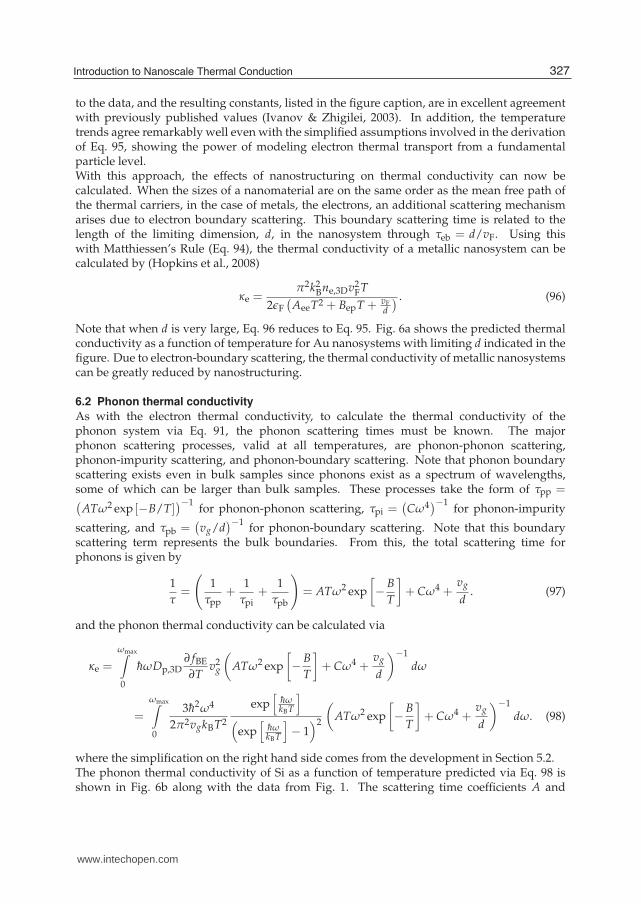
to the data, and the resulting constants, listed in the figure caption, are in excellent agreementwith previously published values (Ivanov & Zhigilei, 2003). In addition, the temperaturetrends agree remarkably well even with the simplified assumptions involved in the derivationof Eq. 95, showing the power of modeling electron thermal transport from a fundamentalparticle level.With this approach, the effects of nanostructuring on thermal conductivity can now becalculated. When the sizes of a nanomaterial are on the same order as the mean free path ofthe thermal carriers, in the case of metals, the electrons, an additional scattering mechanismarises due to electron boundary scattering. This boundary scattering time is related to thelength of the limiting dimension, d, in the nanosystem through τeb = d/vF. Using thiswith Matthiessen’s Rule (Eq. 94), the thermal conductivity of a metallic nanosystem can becalculated by (Hopkins et al., 2008)

κe =π2k2

Bne,3Dv2FT

2ǫF

(

AeeT2 + BepT + vFd

) . (96)

Note that when d is very large, Eq. 96 reduces to Eq. 95. Fig. 6a shows the predicted thermalconductivity as a function of temperature for Au nanosystems with limiting d indicated in thefigure. Due to electron-boundary scattering, the thermal conductivity of metallic nanosystemscan be greatly reduced by nanostructuring.

6.2 Phonon thermal conductivity

As with the electron thermal conductivity, to calculate the thermal conductivity of thephonon system via Eq. 91, the phonon scattering times must be known. The majorphonon scattering processes, valid at all temperatures, are phonon-phonon scattering,phonon-impurity scattering, and phonon-boundary scattering. Note that phonon boundaryscattering exists even in bulk samples since phonons exist as a spectrum of wavelengths,some of which can be larger than bulk samples. These processes take the form of τpp =(

ATω2 exp [−B/T])−1

for phonon-phonon scattering, τpi =(

Cω4)−1

for phonon-impurity

scattering, and τpb =(

vg/d)−1

for phonon-boundary scattering. Note that this boundaryscattering term represents the bulk boundaries. From this, the total scattering time forphonons is given by

1

τ=

(

1

τpp+

1

τpi+

1

τpb

)

= ATω2 exp

[

− B

T

]

+ Cω4 +vg

d. (97)

and the phonon thermal conductivity can be calculated via

κe =

ωmax∫

0

hωDp,3D∂ fBE

∂Tv2

g

(

ATω2 exp

[

− B

T

]

+ Cω4 +vg

d

)−1

dω

=

ωmax∫

0

3h2ω4

2π2vgkBT2

exp[

hωkBT

]

(

exp[

hωkBT

]

− 1)2

(

ATω2 exp

[

− B

T

]

+ Cω4 +vg

d

)−1

dω. (98)

where the simplification on the right hand side comes from the development in Section 5.2.The phonon thermal conductivity of Si as a function of temperature predicted via Eq. 98 isshown in Fig. 6b along with the data from Fig. 1. The scattering time coefficients A and


www.intechopen.com

24 Heat Transfer

322 3222322

622

Vgorgtcvwtg"*M+

Vjgto

cn"Eq

pfwevkxkv{"*Y

"o/3 "M/

3 +

3 32 322 32223

32

322

3222

Vgorgtcvwtg"*M+

Vjgto

cn"Eq

pfwevkxkv{"*Y

"o/3 "M/

3 +

*c+"Cw *d+"Uk

f"?"72"po322"po

722"po

8222

3"│o

f"?"72"po

722"po3"│o

dwnm"oqfgn"*fcujgf+

dwnm"fcvc"*uqnkf+

322"po

dwnm"oqfgn"*fcujgf+dwnm"fcvc"*uqnkf+

Fig. 6. (a) Electron thermal conductivity of Au as a function of temperature for bulk Au andfor Au nanosystems of various limiting sizes indicated in the plot. The bulk modelpredictions, calculated via Eq. 95, are compared to the experimental data in Fig. 1. For these

calculations, Aee = 2.4 × 107 K−2 s−1 and Bep = 1.23 × 1011 K−1 s−1 were assumed, inexcellent agreement with literature values (Ivanov & Zhigilei, 2003). Additionalthermophysical parameters used for this calculation are listed in the caption of Fig. 5. Thevarious Au nanosystem thermal conductivity is calculated via Eq. 96. (b) Phonon thermalconductivity of Si as a function of temperature for bulk Si and for Si nanoysstems of variouslimiting sizes in indicated in the plots. The bulk model predictions, calculated via Eq. 98, arecompared to the experimental data in Fig. 1. For these calculations, the scattering coefficients

were A = 1.23 × 10−19 s K−1, B = 140K, and C = 1.32 × 10−45 s3. In addition, the groupvelocity of Si is taken as the speed of sound, vg = 8,433m s−1, and the lattice parameter of Si

is a = 5.430 × 10−10 m. To fit the bulk data, d = 8.0 × 10−3 m. To examine the effects ofnanostructuring, d is varied as indicated in the plot.

B were iterated to match the data after the maximum and C was taken from the literature(Mingo, 2003). The boundary scattering constant, d, is used as a fitting parameter to match thedata at temperatures lower than the maximum. The resulting coefficients were in excellentagreement with the literature values for bulk Si (Mingo, 2003). Note that the model usingEq. 98 fits the data and captures the temperature trends extremely well showing the powerof modeling the bulk phonon thermal conductivity from a fundamental energy carrier level.To examine the effects of nanostructuring on the phonon thermal conductivity, d is variedto dimensions indicated in Fig. 6b. Nanostructruing greatly reduces the phonon thermalconductivity, especially at low temperatures where phonon mean free paths are long.

7. Summary

Modern devices, with feature sizes on the length scale of electron and phonon meanfree paths, require thermal analyses different from that of the phenomenological FourierLaw. This is due to the fact that the scattering of electrons and phonons in such systemsoccurs predominantly at interfaces, inclusions, grain boundaries, etc., rather than withinthe materials comprising the device themselves. Here, electrons and phonons have beendescribed in terms of their respective dispersion diagrams, calculated via the Schrordingerequation for electrons and atomic equations of motion for phonons. Using this information


www.intechopen.com


and density of states expressions, energy storage properties, i.e., internal energy and heatcapacity, have been formulated. Lastly, applying the Kinetic Theory of Gases, the thermalconductivity expressions for metals and semiconductors have been derived. It has beenshown that limiting feature sizes can result in a significant reduction in thermal conductivity.This, then, once again reinforces the idea that thermal transport on the nanoscale requires analtogether different approach from that at the macroscale.

8. Acknowledgements

The authors would like to acknowledge Professor Pamela M. Norris at the University ofVirginia for helpful advice and for recommending the writing of this book chapter. P.E.H.would like to thank Dr. Leslie M. Phinney at Sandia National Laboratories for guidanceand support. P.E.H. is appreciative for funding from the LDRD program office through theSandia National Laboratories Harry S. Truman Fellowship Program. J.C.D. is appreciativefor funding from the National Science Foundation Graduate Research Fellowship Program.Sandia is a multiprogram laboratory operated by Sandia Corporation, a wholly ownedsubsidiary of Lockheed Martin Corporation, for the United States Department of Energy’sNational Nuclear Security Administration under Contract DE-AC04-94AL85000.

9. References

Cahill, D. G., Ford, W. K., Goodson, K. E., Mahan, G. D., Majumdar, A., Maris, H. J., Merlin,R. & Phillpot, S. R. (2003). Nanoscale thermal transport, Journal of Applied Physics93(2): 793–818.

Chen, G. (2005). Nanoscale Energy Transport and Conversion: A Parallel Treatment of Electrons,Molecules, Phonons, and Photons, Oxford University Press, New York, New York.

Dove, M. T. (1993). Introduction to Lattice Dynamics, number 4 in Cambridge Topics in MineralPhysics and Chemistry, Cambridge University Press, Cambridge, England.

Griffiths, D. (2000). Introduction to Quantum Mechanics, 2nd edn, Prentice Hall, Upper SaddleRiver, New Jersey.

Ho, C. Y., Powell, R. W. & Liley, P. E. (1972). Thermal conductivity of the elements, Journal ofPhysical and Chemical Reference Data 1(2): 279–421.

Hopkins, P. E., Norris, P. M., Phinney, L. M., Policastro, S. A. & Kelly, R. G. (2008). Thermalconductivity in nanoporous gold films during electron-phonon nonequilibrium,Journal of Nanomaterials (418050).

Ivanov, D. S. & Zhigilei, L. V. (2003). Combined atomistic-continuum modeling of short-pulselaser melting and disintegration, Physical Review B 68: 064114.

Kittel, C. (2005). Introduction to Solid State Physics, 8th edn, Wiley, Hoboken, New Jersey.Mingo, N. (2003). Calculation of Si nanowire thermal conductivity using complete phonon

dispersion relations, Physical Review B 68(11): 113308.Schrodinger, E. (1926). Quantisation as a problem of characteristic values, Annalan der Physik

79: 361–376, 489–527.Srivastava, G. P. (1990). The Physics of Phonons, Adam Hilger, Bristol, England.Tien, C.-L., Majumdar, A. & Gerner, F. M. (1998). Microscale Energy Transport, Taylor and

Francis, Washington, D.C.Vincenti, W. G. & Kruger, C. H. (2002). Introduction to Physical Gas Dynamics, Krieger

Publishing Company, Malabar, Florida.Wolf, E. L. (2006). Nanophysics and Nanotechnology: An Introduction to Modern Concepts in


www.intechopen.com

26 Heat Transfer

Nanoscience, 2nd edn, WILEY-VCH Verlag GmbH & Co. KGaA, Weinheim, Germany.Ziman, J. M. (1972). Principles of the Theory of Solids, 2nd edn, Cambridge University Press,

Cambridge, England.


www.intechopen.com

Heat Transfer - Mathematical Modelling, Numerical Methods andInformation TechnologyEdited by Prof. Aziz Belmiloudi

ISBN 978-953-307-550-1Hard cover, 642 pagesPublisher InTechPublished online 14, February, 2011Published in print edition February, 2011

InTech EuropeUniversity Campus STeP Ri Slavka Krautzeka 83/A 51000 Rijeka, Croatia Phone: +385 (51) 770 447 Fax: +385 (51) 686 166

InTech ChinaUnit 405, Office Block, Hotel Equatorial Shanghai No.65, Yan An Road (West), Shanghai, 200040, China

Phone: +86-21-62489820 Fax: +86-21-62489821

Over the past few decades there has been a prolific increase in research and development in area of heattransfer, heat exchangers and their associated technologies. This book is a collection of current research inthe above mentioned areas and describes modelling, numerical methods, simulation and informationtechnology with modern ideas and methods to analyse and enhance heat transfer for single and multiphasesystems. The topics considered include various basic concepts of heat transfer, the fundamental modes ofheat transfer (namely conduction, convection and radiation), thermophysical properties, computationalmethodologies, control, stabilization and optimization problems, condensation, boiling and freezing, with manyreal-world problems and important modern applications. The book is divided in four sections : "Inverse,Stabilization and Optimization Problems", "Numerical Methods and Calculations", "Heat Transfer in Mini/MicroSystems", "Energy Transfer and Solid Materials", and each section discusses various issues, methods andapplications in accordance with the subjects. The combination of fundamental approach with many importantpractical applications of current interest will make this book of interest to researchers, scientists, engineers andgraduate students in many disciplines, who make use of mathematical modelling, inverse problems,implementation of recently developed numerical methods in this multidisciplinary field as well as toexperimental and theoretical researchers in the field of heat and mass transfer.

How to referenceIn order to correctly reference this scholarly work, feel free to copy and paste the following:

Patrick E. Hopkins and John C. Duda (2011). Introduction to Nanoscale Thermal Conduction, Heat Transfer -Mathematical Modelling, Numerical Methods and Information Technology, Prof. Aziz Belmiloudi (Ed.), ISBN:978-953-307-550-1, InTech, Available from: http://www.intechopen.com/books/heat-transfer-mathematical-modelling-numerical-methods-and-information-technology/introduction-to-nanoscale-thermal-conduction

www.intechopen.com

www.intechopen.com

Documents

Introduction to Nanoscale Thermal Conduction · PDF file0 Introduction to Nanoscale Thermal Conduction Patrick E. Hopkins1,2 and John C. Duda2 1Sandia National Laboratories, Albuquerque,