Introduction to Loop Quantum Gravity

Abhay Ashtekar

Institute for Gravitation and the Cosmos, Penn State

A broad perspective on the challenges, structure and successes of loop quantum gravity.

Focus on conceptual issues, coherence of physical principles and viability of predictions

CUP Monographs by Carlo Rovelli (2004) and Thomas Thiemann (2008);

Introduction: Gravity and the Quantum by AA, New J.Phys. 7 (2005) 198

Overview Lecture for PHY565

– p.

Organization

1. Historical and Conceptual Setting2. Loop Quantum Gravity: Quantum Geometry3. Black Holes: Zooming in on Quantum Geometry4. Big Bang: Loop Quantum Cosmology5. Summary

– p.

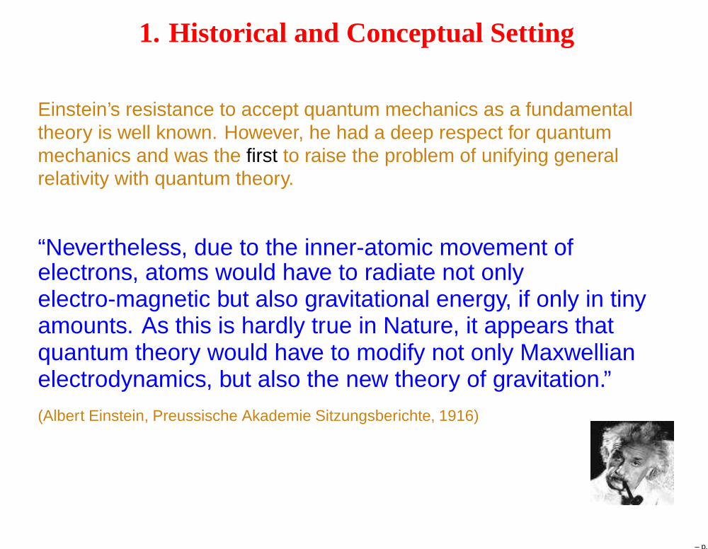
1. Historical and Conceptual Setting

Einstein’s resistance to accept quantum mechanics as a fundamentaltheory is well known. However, he had a deep respect for quantummechanics and was the first to raise the problem of unifying generalrelativity with quantum theory.

“Nevertheless, due to the inner-atomic movement ofelectrons, atoms would have to radiate not onlyelectro-magnetic but also gravitational energy, if only in tinyamounts. As this is hardly true in Nature, it appears thatquantum theory would have to modify not only Maxwellianelectrodynamics, but also the new theory of gravitation.”

(Albert Einstein, Preussische Akademie Sitzungsberichte, 1916)

– p.

• Physics has advanced tremendously in the last 90 years but the theproblem of unification of general relativity and quantum physics still open.Why?⋆ No experimental data with direct ramifications on the quantum nature ofGravity.

– p.

• Physics has advanced tremendously in the last 90 years but the theproblem of unification of general relativity and quantum physics still open.Why?⋆ No experimental data with direct ramifications on the quantum nature ofGravity.⋆ But then this should be a theorist’s haven! Why isn’t there a plethora oftheories?

– p.

• Physics has advanced tremendously in the last 90 years but the theproblem of unification of general relativity and quantum physics still open.Why?⋆ No experimental data with direct ramifications on quantum Gravity.⋆ But then this should be a theorist’s haven! Why isn’t there a plethora oftheories?

• In general relativity, gravity is coded in space-time geometry. Mostspectacular predictions —e.g., the Big-Bang, Black Holes & GravitationalWaves— emerge from this encoding. Suggests: Geometry itself mustbecome quantum mechanical. How do you do physics without aspace-time continuum in the background?

• Several approaches: Causal sets, twistors, AdS/CFTconjecture of string theory. Loop Quantum Gravity grewout of the Hamiltonian approach pioneered by Bergmann,Dirac, and developed by Wheeler, DeWitt and others.

– p.

Contrasting LQG with String theory

Because there are no direct experimental checks, approaches are drivenby intellectual prejudices about what the core issues are and what will“take care of itself” once the core issues are resolved.

Particle Physics: ‘Unification’ Central: Extend Perturbative, flat spaceQFTs; Gravity just another force.• Higher derivative theories; • Supergravity• String theory incarnations:⋆ Perturbative strings; ⋆ M theory & F theory;⋆ Matrix Models; ⋆ AdS/CFT Correspondence.

– p.

Contrasting LQG with String theory

• Particle Physics: ‘Unification’ Central: Extend Perturbative, flat spaceQFTs; Gravity just another force.• Higher derivative theories; • Supergravity• String theory incarnations:⋆ Perturbative strings; ⋆ M theory;⋆ Matrix Models; ⋆ AdS/CFT Correspondence.

• General Relativity: ‘Background independence’ Central: LQG⋆ Quantum Geometry (Hamiltonian Theory used for cosmology & BHs),⋆ Spin-foams (Path integrals used to bridge low energy physics.)

Issues:• Unification: Ideas proposed in LQG but strong limitations;Recall however, QCD versus Grand Unified Theories.• Background Independence: Progress through AdS/CFT; but a ‘smallcorner’ of QG; Physics beyond singularities and S-matrices?

A. Ashtekar: LQG: Four Recent Advances and a dozen FAQs;

arXiv:0705.2222

– p.

Organization

1. Historical and Conceptual Setting2. Loop Quantum Gravity: Quantum Geometry3. Black Holes: Zooming in on Quantum Geometry4. Big Bang: Loop Quantum Cosmology5. Summary

– p.

2. Loop Quantum Gravity: Quantum Geometry

• Geometry: Physical entity, as real as tables and chairs.Riemann 1854: Göttingen Address; Einstein 1915: General Relativity

• Matter has constituents. GEOMETRY??‘Atoms of Geometry’? Why then does the continuum picture work so well?Are there physical processes which convert Quanta of Geometry toQuanta of Matter and vice versa?

– p. 10

2. Loop Quantum Gravity: Quantum Geometry

• A Paradigm shift to address these issues

“The major question for anyone doing research in this field is: Of which mathematical typeare the variables . . . which permit the expression of physical properties of space. . . Onlyafter that, which equations are satisfied by these variables?” Albert Einstein(1946); Autobiographical Notes.

• Choice in General Relativity: Metric, gµν . Directly determinesRiemannian geometry; Geometrodynamics.In all other interactions, by contrast, the basic variable is a Connection,i.e., a matrix valued vector potential Ai

a;Gauge theories: Connection-dynamics

• Key new idea: Cast GR also as a theory of connections. Import into GRtechniques from gauge theories. ‘Kinematic unification’(AA, 1986)

– p. 11

Holonomies/Wilson Lines and Frames/Triads

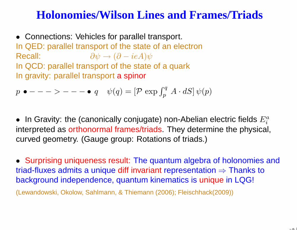
• Connections: Vehicles for parallel transport.In QED: parallel transport of the state of an electronRecall: ∂ψ → (∂ − ieA)ψIn QCD: parallel transport of the state of a quarkIn gravity: parallel transport a chiral spinor

p • − −− > −−− • q ψ(q) = [P exp∫ q

pA · dS]ψ(p)

• In Gravity: the (canonically conjugate) non-Abelian electric fields Eai

interpreted as orthonormal frames/triads. They determine the physical,curved geometry. (Gauge group: Rotations of triads.)

– p. 12

Holonomies/Wilson Lines and Frames/Triads

• Connections: Vehicles for parallel transport.In QED: parallel transport of the state of an electronRecall: ∂ψ → (∂ − ieA)ψIn QCD: parallel transport of the state of a quarkIn gravity: parallel transport a spinor

p • − −− > −−− • q ψ(q) = [P exp∫ q

pA · dS]ψ(p)

• In Gravity: the (canonically conjugate) non-Abelian electric fields Eai

interpreted as orthonormal frames/triads. They determine the physical,curved geometry. (Gauge group: Rotations of triads.)

• Surprising uniqueness result: The quantum algebra of holonomies andtriad-fluxes admits a unique diff invariant representation ⇒ Thanks tobackground independence, quantum kinematics is unique in LQG!

(Lewandowski, Okolow, Sahlmann, & Thiemann (2006); Fleischhack(2009))

– p. 13

Polymer Geometry

• This unique kinematics was first constructed explicitly in the early1990s. High mathematical precision. Provides a Quantum Geometry.Replaces the Riemannian geometry used in classical gravity theories.AA, Baez, Corichi, Lewandowski, Marolf, Mourão, Rovelli, Smolin, Thiemann, Zapata,...

• Quantum States: Ψ ∈ H = L2(A, dµo)

µo a diffeomorphism invariant, regular measure on the space A of(generalized) connections.

• Fundamental excitations of geometry 1-dimensional. Polymer geometryat the Planck scale. Continuum arises only in the coarse rainedapproximation.

– p. 14

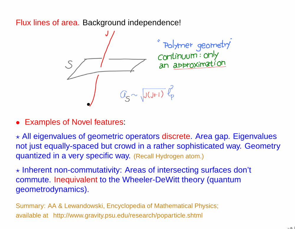
Flux lines of area. Background independence!

• Examples of Novel features:

⋆ All eigenvalues of geometric operators discrete. Area gap. Eigenvaluesnot just equally-spaced but crowd in a rather sophisticated way. Geometryquantized in a very specific way. (Recall Hydrogen atom.)

⋆ Inherent non-commutativity: Areas of intersecting surfaces don’tcommute. Inequivalent to the Wheeler-DeWitt theory (quantumgeometrodynamics).

Summary: AA & Lewandowski, Encyclopedia of Mathematical Physics;

available at http://www.gravity.psu.edu/research/poparticle.shtml

– p. 15

Organization

1. Historical and Conceptual Setting2. Loop Quantum Gravity: Quantum Geometry3. Black Holes: Zooming in on Quantum Geometry4. Big Bang: Loop Quantum Cosmology5. Summary

– p. 16

3. Black Holes: Zooming in on Quantum Geometry

• First law of BH Mechanics + Hawking’s discovery that TBH = κ~/2π ⇒for large BHs, SBH = ahor/4ℓpl

2 (Bekenstein 1973)

• Entropy: Why is the entropy proportional to area? For a M⊙ black hole,we must have exp 1076 micro-states, a HUGE number even by standardsof statistical mechanics. Where do these micro-states come from?

For gas in box, the microstates come from molecules; for a ferromagnet,from Heisenberg spins; Black hole ?Cannot be gravitons: gravitational fields stationary.

• To answer these questions, must go beyond the classical space-timeapproximation used in the Hawking effect. Must take into account thequantum nature of gravity.

• Distinct approaches. In Loop Quantum Gravity, this entropy arises fromthe huge number of microstates of the quantum horizon geometry.‘Atoms’ of geometry itself!

– p. 17

Quantum Horizon Geometry & Entropy

• Heuristics: Wheeler’s It from BitDivide the horizon into elementary cells, each carrying area ℓpl

2.Assign to each cell a ‘Bit’ i.e. 2 states.Then, # of cells n ∼ ao/ℓpl

2; No of states N ∼ 2n;Shor ∼ lnN ∼ n ln 2 ∼ ao/ℓpl

2. Thus, Shor ∝ ao/ℓpl2.

• Argument made rigorous in quantum geometry. Many inaccuracies ofthe heuristic argument have to be overcome: Quanta of area not ℓpl

2 but

4πγ√j(j+) ℓpl

2; Calculation has to know that the surface is black holehorizon; What is a quantum horizon?

• Interesting mathematical structures U(1) Chern-Simons theory;non-commutative torus, quantum U(1), mapping class group, ...(AA, Baez, Krasnov)

– p. 18

Quantum Horizon

Polymer excitations of geometry in the bulk puncture the horizon.Quantum horizon geometry described by the U(1) Chern-Simons theory.

– p. 19

Quantum Horizon Geometry and Entropy

• Horizon geometry flat everywhere except at punctures. At puncturesthe bulk polymer excitations cause a ‘tug’ giving rise to quantized deficitangles. They add up to 4π providing a 2-sphere quantum geometry.‘Quantum Gauss-Bonnet Theorem’.

• As in Statistical mechanics,have to construct a suitable ensemble ρ by specifyingmacroscopic parameters (multipoles) characterizingthe classical horizon geometry. Shor = Trρ ln ρgives the log of the number of quantum horizongeometry states compatible with the classical geometry.

• Shor = ahor/4ℓpl2 − (1/2) ln(ahor/ℓpl

2) + o(ahor/ℓpl2)

gamma

pi

for a specific value of the parameter γ ≈ 0.24.Procedure incorporates all physically interestingBHs and Cosmological horizons in one swoop.

(AA, Baez, Krasnov; Domagala, Lewandowski; Meissner;

AA, Engle, Van Den Broeck)

– p. 20

Organization

1. Historical and Conceptual Setting2. Loop Quantum Gravity: Quantum Geometry3. Black Holes: Zooming in on Quantum Geometry4. Big Bang: Loop Quantum Cosmology5. Summary

– p. 21

4. Big-Bang: Loop Quantum Cosmology

• Issue: In classical General Relativity, assumption of spatialhomogeneity & isotropy implies that the metric has the FLRW form;a(t): Scale FactorVolume ∼ [a(t)]3 Curvature ∼ [a(t)]−n

Einstein Equations ⇒ volume → 0 and Curvature → ∞: BIG BANG!!Classical SPACE-TIME ENDS; PHYSICS STOPS!!

– p. 22

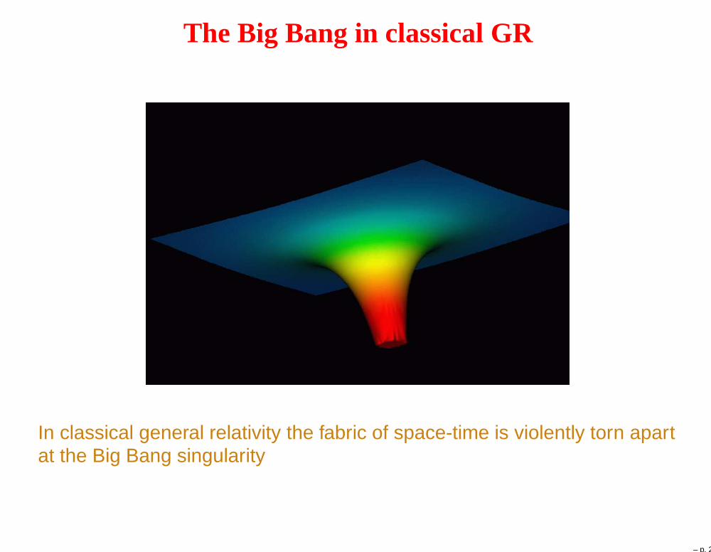
The Big Bang in classical GR

In classical general relativity the fabric of space-time is violently torn apartat the Big Bang singularity

– p. 23

• Expectation: Just an indication that the theory is pushed beyond itsdomain of validity.Example: H-atom. Energy unbounded below in the classical theory;

instability. Quantum theory: Eo = −me4

2~2

• Is this the case? If so, what is the true physics near the Big Bang?Need a theory which can handle both strong gravity/curvature andquantum physics, i.e., Quantum Gravity.Scale for new phenomena: ℓPl = (G~/c3)

1

2 ∼ 10−33cm

– p. 24

• Some Long-Standing Questions expected to be answered by QuantumGravity from first principles:

⋆ Is the Big-Bang singularity naturally resolved by quantum gravity? Or,Is a new principle/ boundary condition at the Big Bang essential?⋆ Is the quantum evolution across the ‘singularity’ deterministic?(answer ‘No’ e.g. in the Pre-Big-Bang and Ekpyrotic scenarios)

⋆ What is on the other side? A quantum foam? Another large, classicaluniverse? ...

– p. 25

• Some Long-Standing Questions expected to be answered by QuantumGravity from first principles:

⋆ Is the Big-Bang singularity naturally resolved by quantum gravity? Or,Is a new principle/ boundary condition at the Big Bang essential?⋆ Is the quantum evolution across the ‘singularity’ deterministic?(answer ‘No’ e.g. in the Pre-Big-Bang and Ekpyrotic scenarios)

⋆ What is on the other side? A quantum foam? Another large, classicaluniverse? ...

• Emerging Scenario: vast classical regions bridged deterministically byquantum geometry. No new principle needed.(AA, Bojowald, Chiou, Corichi, Pawlowski, Singh, Vandersloot,... )

• In the classical theory, don’t need full Einstein equations in all theircomplexity. Almost all work in physical cosmology based onhomogeneous isotropic models and perturbations thereon. At least in afirst step, can use the same strategy in the quantum theory: mini andmidi-superspaces.

– p. 26

A Simple ModelA FRW Model: Gravity coupled to a massless scalar field φ. Instructivebecause every classical solution is singular. Provides a foundation formore complicated models.

-1.2

-1

-0.8

-0.6

-0.4

-0.2

0

0 1*104 2*104 3*104 4*104 5*104

v

φ

Classical trajectories

– p. 27

Older Quantum Cosmology (DeWitt, Misner, . . . 70’s)

• Since only finite number of DOF a(t), φ(t), field theoretical difficultiesbypassed; analysis reduced to standard quantum mechanics.

• Quantum States: Ψ(a, φ); aΨ(a, φ) = aΨ(a, φ) etc.Quantum evolution governed by the Wheeler-DeWitt equation on Ψ(a, φ)Without additional assumptions, singularity is not resolved by theequation.

• General belief since late seventies: This situation can not be remediedbecause of von-Neumann’s uniqueness theorem which lies at the heart ofQM.

• New Development: A key assumption of the theorem fails in LQG⇒ von-Neumann’s uniqueness result naturally bypassed.

(AA, Bojowald, Lewandowski).New Quantum Mechanics! (H 6= L2(R) but rather H = L2(RBohr).)Novel features precisely in the deep Planck regime.

– p. 28

-1.2

-1

-0.8

-0.6

-0.4

-0.2

0

0 1*104 2*104 3*104 4*104 5*104

v

φ

Classical trajectories

– p. 29

-1.2

-1

-0.8

-0.6

-0.4

-0.2

0

0 1*104 2*104 3*104 4*104 5*104

v

φ

LQCclassical

Expectations values and dispersions of V |φ & classical trajectories.

– p. 30

0

0.2

0.4

0.6

0.8

1

1.2

1.4

1.6

-1.2

-1

-0.8

-0.6

-0.4

-0.2

5*103

1.0*104

1.5*104

2.0*104

2.5*104

3.0*104

3.5*104

4.0*104

0

0.5

1

1.5

|Ψ(v,φ)|

v

φ

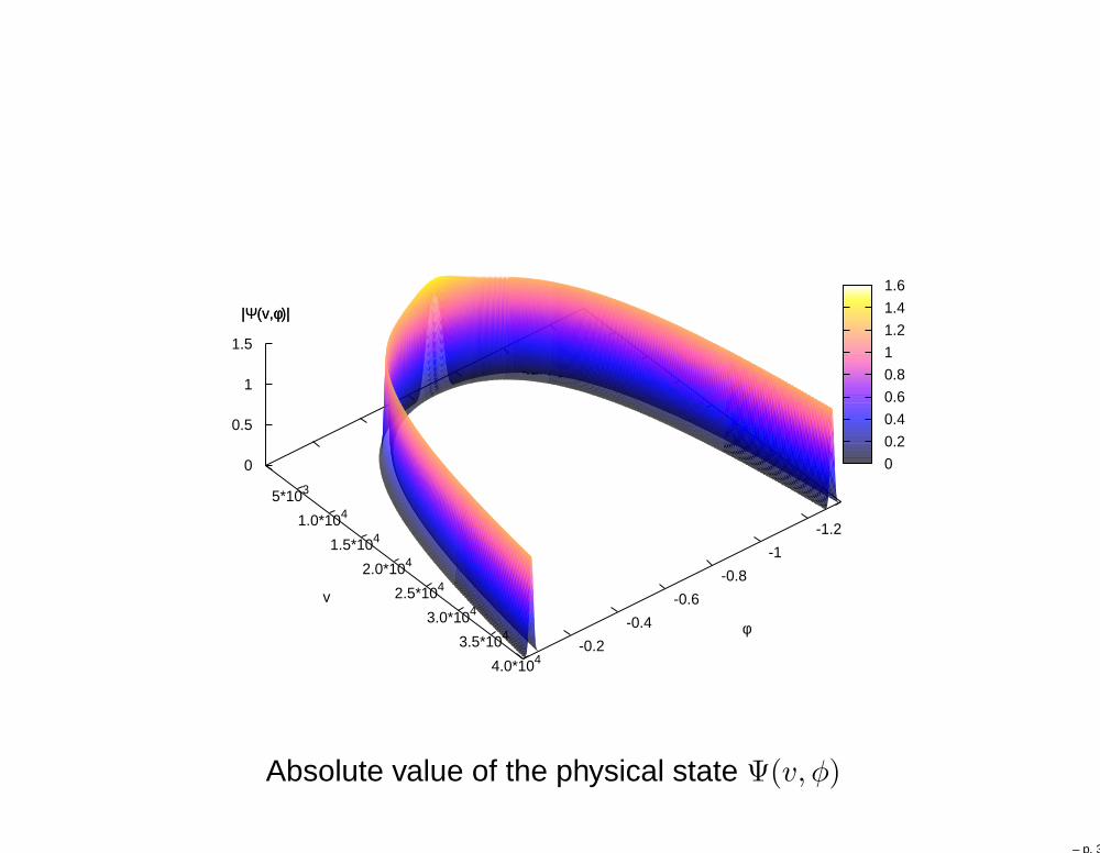
|Ψ(v,φ)|

Absolute value of the physical state Ψ(v, φ)

– p. 31

Results

Assume that the quantum state is semi-classical at late times (e.g., NOW)and evolve backwards. Then:

• The state remains semi-classical till very early times! Till ρ ∼ ρPl. ⇒Space-time can be taken to be classical during the inflationary era.

• In the deep Planck regime, semi-classicality fails. But quantumevolution is well-defined through the Planck regime, and remainsdeterministic. No new principle needed.

– p. 32

ResultsAssume that the quantum state is semi-classical at late times (e.g., NOW)and evolve backwards. Then:

• The state remains semi-classical till very early times! Till ρ ∼ ρPl. ⇒Space-time can be taken to be classical during the inflationary era.

• In the deep Planck regime, semi-classicality fails. But quantumevolution is well-defined through the Planck regime, and remainsdeterministic. No new principle needed.

• Big bang replaced by a quantum bounce. Matter satisfies standardenergy conditions. Exact quantum analysis using semi-classical states notWKB. Quantum geometry ‘bridges’ an infinite expanding branch with aninfinite contracting branch.

• A new ‘repulsive force’ due to quantum geometry. Unlike in otherapproaches with bounces, unambiguous evolution across the ‘bridge’,provided by the quantum Einstein equation. Effective Friedmann Eq:

(a/a)2 = (8πGρ/3) [1 − ρ/ρcrit] with ρcrit ≈ 0.4ρPlanck

• Results robust for all simple models (open, closed, Λ = 0,Λ > 0,Λ < 0,anisotropies).

– p. 33

The Big Bang in classical GR

In classical general relativity the fabric of space-time is violently torn apartat the Big Bang singularity

– p. 34

The Big Bang in LQC

In loop quantum cosmology our post-big-bang branch of the universe isjoined to a pre-big-bang branch by a quantum bridge.

– p. 35

Summary and Outlook

• In Loop Quantum Gravity, the interplay between geometry and physicsis elevated to quantum level. Just as general relativity is based onRiemannian geometry, LQG is based on a specific quantum geometry.

• Quantum geometry effects negligible under ‘normal conditions’ butdominate physics at Planck scale. Physics does not end at classicalsingularities. Many long standing fundamental questions answered both incosmology and in black hole physics.

• Singularity resolution ⇒ the quantum space-time is vastly larger thanwhat GR had us believe. This also provides a novel avenue to resolve the‘information loss’ issue.

• So far focus has been on conceptual challenges. Just beginning tograpple with the all important phenomenological issues. Interestingchallenges and overlap with mathematics, lattice gauge theories, QFT,GR, cosmology, & computational physics.

– p. 36

k=1 Model: WDW Theory

-2

-1.5

-1

-0.5

0

0.5

1

1.5

2

0 1*104 2*104 3*104 4*104 5*104 6*104 7*104 8*104 9*104 1.0*105

φ

v

WDWclassical

Expectations values and dispersions of V |φ.

– p. 37

k=1 Model: LQC

-5

-4

-3

-2

-1

0

0 2*104 4*104 6*104 8*104 1.0*105

φ

v

LQCEffectiveClassical

Expectations values and dispersions of V |φ & classical trajectories.(AA, Pawlowski, Singh, Vandersloot)

– p. 38

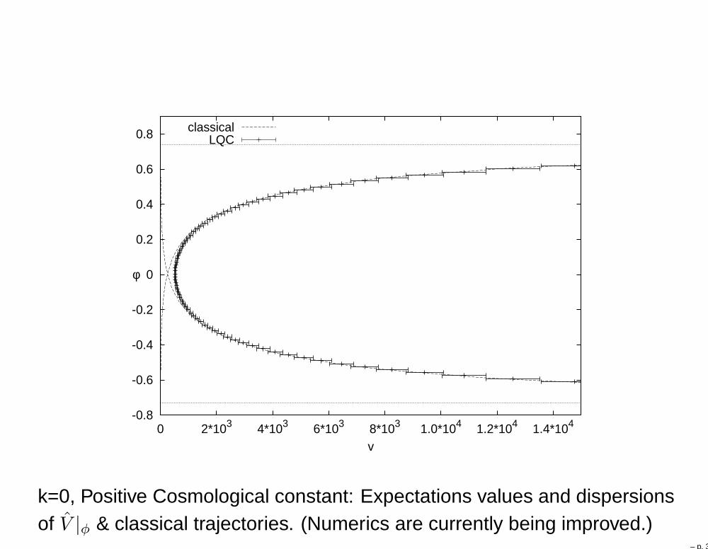
-0.8

-0.6

-0.4

-0.2

0

0.2

0.4

0.6

0.8

0 2*103 4*103 6*103 8*103 1.0*104 1.2*104 1.4*104

v

φ

classicalLQC

k=0, Positive Cosmological constant: Expectations values and dispersionsof V |φ & classical trajectories. (Numerics are currently being improved.)

– p. 39

-3

-2.5

-2

-1.5

-1

-0.5

0

0 2*104 4*104 6*104 8*104 1.0*105 1.2*105

v

φ

classicalLQC

k=0, Negative Cosmological constant: Expectations values and– p. 40

Quantum Theory

Finite number of degrees of freedom ⇒ Quantum Mechanics.If x, p is the canonically conjugate pair, [x, p] = i I.If U(λ) = eiλx and V (µ) = eiµp, then U(λ) V (µ) = eiλµ V (µ) U(λ).

von Neumann’s uniqueness theorem: There is a unique IRR ofU(λ), V (µ) by 1-parameter unitary groups on a Hilbert space satisfying:i) commutation relations; and ii) Weak continuity in λ, µ.This is the standard Schrödinger representation.

– p. 41

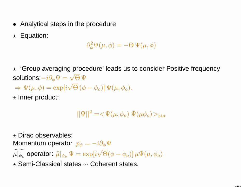
• Analytical steps in the procedure

⋆ Equation:∂2

φΨ(µ, φ) = −Θ Ψ(µ, φ)

⋆ ‘Group averaging procedure’ leads us to consider Positive frequencysolutions:−i∂φΨ =

√Θ Ψ

⇒ Ψ(µ, φ) = exp[i√

Θ (φ− φo)] Ψ(µ, φo).

⋆ Inner product:

||Ψ||2 =<Ψ(µ, φo) Ψ(µφo)>kin

⋆ Dirac observables:Momentum operator pφ = −i∂φΨ

µ|φooperator: µ|φo

Ψ = exp[i√

Θ(φ− φo)]µΨ(µ, φo)

⋆ Semi-Classical states ∼ Coherent states.

– p. 42

Basic Strategy

• Analytical Issues: the quantum Hamiltonian constraint takes the form:

−Θ Ψ(v, φ) = ∂2φΨ(v, φ) (⋆)

where Θ is a self-adjoint difference operator independent of φ:

Θ Ψ(v, φ) = C+(v)ψ(v + 4, φ) + Co(v)ψ(v, φ) + C−(v)ψ(v, φ)

suggests φ could be used as ‘emergent time’ also in the quantum theory.

Strategy: Physical states: solutions to (⋆). Observables: V |φ=φoand p|φ.

Inner product: Makes these self-adjoint. Semi-classical states:Generalized coherent states.

• Use numerical methods to solve the Quantum Constraint. Severalsubtleties had to be carefully handled.

– p. 43