Embed Size (px)
Citation preview

Covariant Loop Quantum GravityAn elementary introduction to Quantum Gravity and Spinfoam Theory
CARLO ROVELLI AND FRANCESCA VIDOTTO


iii
.
Cover: Martin Klimas, ”Jimi Hendrix, House Burning Down”.

Contents
Preface page ix
Part I Foundations 1
1 Spacetime as a quantum object 31.1 The problem 31.2 The end of space and time 61.3 Geometry quantized 91.4 Physical consequences of the existence of the Planck scale 18
1.4.1 Discreteness: scaling is finite 181.4.2 Fuzziness: disappearance of classical space and time 19
1.5 Graphs, loops and quantum Faraday lines 201.6 The landscape 221.7 Complements 24
1.7.1 SU(2) representations and spinors 241.7.2 Pauli matrices 271.7.3 Eigenvalues of the volume 29
2 Physics without time 312.1 Hamilton function 31
2.1.1 Boundary terms 352.2 Transition amplitude 36
2.2.1 Transition amplitude as an integral over paths 372.2.2 General properties of the transition amplitude 40
2.3 General covariant form of mechanics 422.3.1 Hamilton function of a general covariant system 452.3.2 Partial observables 462.3.3 Classical physics without time 47
2.4 Quantum physics without time 482.4.1 Observability in quantum gravity 512.4.2 Boundary formalism 522.4.3 Relational quanta, relational space 54
2.5 Complements 552.5.1 Example of timeless system 552.5.2 Symplectic structure and Hamilton function 57
iv

v Contents
3 Gravity 593.1 Einstein’s formulation 593.2 Tetrads and fermions 60
3.2.1 An important sign 633.2.2 First-order formulation 64
3.3 Holst action and Barbero-Immirzi coupling constant 653.3.1 Linear simplicity constraint 673.3.2 Boundary term 68
3.4 Hamiltonian general relativity 693.4.1 ADM variables 693.4.2 What does this mean? Dynamics 713.4.3 Ashtekar connection and triads 73
3.5 Euclidean general relativity in three spacetime dimensions 763.6 Complements 78
3.6.1 Working with general covariant field theory 783.6.2 Problems 81
4 Classical discretization 824.1 Lattice QCD 82
4.1.1 Hamiltonian lattice theory 844.2 Discretization of covariant systems 854.3 Regge calculus 874.4 Discretization of general relativity on a two-complex 914.5 Complements 98
4.5.1 Holonomy 984.5.2 Problems 99
Part II 3d theory 101
5 3d Euclidean theory 1035.1 Quantization strategy 1035.2 Quantum kinematics: Hilbert space 104
5.2.1 Length quantization 1055.2.2 Spin networks 106
5.3 Quantum dynamics: Transition amplitudes 1105.3.1 Properties of the amplitude 1145.3.2 Ponzano-Regge model 115
5.4 Complements 1185.4.1 Elementary harmonic analysis 1185.4.2 Alternative form of the transition amplitude 1195.4.3 Poisson brackets 1215.4.4 Perimeter of the Universe 122

vi Contents
6 Bubbles and cosmological constant 1236.1 Vertex amplitude as gauge-invariant identity 1236.2 Bubbles and spikes 1256.3 Turaev-Viro amplitude 129
6.3.1 Cosmological constant 1316.4 Complements 133
6.4.1 Few notes on SU(2)q 133
Part III The real world 135
7 The real world: 4D Lorentzian theory 1377.1 Classical discretization 1377.2 Quantum states of gravity 140
7.2.1 Yγ map 1417.2.2 Spin networks in the physical theory 1437.2.3 Quanta of space 145
7.3 Transition amplitudes 1477.3.1 Continuum limit 1507.3.2 Relation with QED and QCD 152
7.4 Full theory 1537.4.1 Face-amplitude, wedge-amplitude and the kernel P 1547.4.2 Cosmological constant and IR finiteness 1557.4.3 Variants 156
7.5 Complements 1587.5.1 Summary of the theory 1587.5.2 Computing with spin networks 1607.5.3 Spectrum of the volume 1637.5.4 Unitary representation of the Lorentz group and the Yγ map 166
8 Classical limit 1708.1 Intrinsic coherent states 170
8.1.1 Tetrahedron geometry and SU(2) coherent states 1718.1.2 Livine-Speziale coherent intertwiners 1758.1.3 Thin and thick wedges and time oriented tetrahedra 176
8.2 Spinors and their magic 1778.2.1 Spinors, vectors and bivectors 1788.2.2 Coherent states and spinors 1808.2.3 Representations of SU(2) and SL(2,C) on functions of
spinors and Yγ map 1818.3 Classical limit of the vertex amplitude 183
8.3.1 Transition amplitude in terms of coherent states 1848.3.2 Classical limit versus continuum limit 188
8.4 Extrinsic coherent states 191

vii Contents
9 Matter 1969.1 Fermions 1969.2 Yang-Mills fields 202
Part IV Physical applications 205
10 Black holes 20710.1 Bekenstein-Hawking entropy 20710.2 Local thermodynamics and Frodden-Ghosh-Perez energy 20910.3 Kinematical derivation of the entropy 21110.4 Dynamical derivation of the entropy 214
10.4.1 Entanglement entropy and area fluctuations 21910.5 Complements 220
10.5.1 Accelerated observers in Minkowski and Schwarzshild 22010.5.2 Tolman law and thermal time 22010.5.3 Algebraic quantum theory 22110.5.4 KMS and thermometers 22210.5.5 General covariant statistical mechanics and quantum
gravity 223
11 Cosmology 22611.1 Classical cosmology 22611.2 Canonical Loop Quantum Cosmology 22911.3 Spinfoam Cosmology 231
11.3.1 Homogeneus and isotropic geometry 23211.3.2 Vertex expansion 23311.3.3 Large-spin expansion 234
11.4 Maximal acceleration 23611.5 Physical predictions? 237
12 Scattering 23812.1 n-point functions in general covariant theories 23812.2 Graviton propagator 242
13 Final remarks 24713.1 Brief historical note 24713.2 What is missing 248
Index 252
References 252Index 265

Preface
To ours teachers and all those who teach children to question ourknowledge, learn through collaboration and the joy of discovery.
This book is an introduction to loop quantum gravity (LQG) focusing on its co-variant formulation. The book has grown from a series of lectures given by CarloRovelli and Eugenio Bianchi at Perimeter Institute during April 2012 and a coursegiven by Rovelli in Marseille in the winter 2013. The book is introductory, and as-sumes only some basic knowledge of general relativity, quantum mechanics andquantum field theory. It is simpler and far more readable than the loop quantumgravity text “Quantum Gravity” [Rovelli (2004)], and the advanced and condensed“Zakopane lectures” [Rovelli (2011)], but it covers, and in facts focuses, on the mo-mentous advances in the covariant theory developed in the last few years, whichhave lead to finite transition amplitudes and were only foreshadowed in [Rovelli(2004)].
There is a rich literature on LQG, to which we refer for all the topics not coveredin this book. On quantum gravity in general, Claus Kiefer has a recent general in-troduction [Kiefer (2007)]. Ashtekar and Petkov are editing a ”Springer Handbookof Spacetime” [Ashtekar and Petkov (2013)], with numerous useful contributions,including John Engle article on spinfoams.
A fine book with much useful background material is John Baez and Javier Mu-nian’s [Baez and Munian (1994)]. By John Baez, see also [Baez (1994b)], with manyideas and a nice introduction to the subject. An undergraduate level introductionto LQG is provided by Rodolfo Gambini and Jorge Pullin [Gambini and Pullin(2010)]. A punctilious and comprehensive text on the canonical formulation of thetheory, rich in mathematical details, is Thomas Thiemann’s [Thiemann (2007)]. Thevery early form of the theory and the first ideas giving rise to it can be found inthe 1991 book by Abhay Ashtekar [Ashtekar (n.d.)].
A good recent reference is the collection of the proceedings of the 3rd Zakopaneschool on loop quantum gravity, organized by Jerzy Lewandowski [Barrett et al.(2011a)]. It contains an introduction to LQG by Abhay Ashtekar [Ashtekar (2011)],Rovelli’s “Zakopane lectures” [Rovelli (2011)], the introduction by Kristina Gieseland Hanno Sahlmann to the canonical theory, and John Barrett et al review on thesemiclassical approximation to the spinfoam dynamics [Barrett et al. (2011b)]. Wealso recommend Alejandro Perez spinfoam review [Perez (2012)], which is com-plementary to this book in several way. Finally, we recommend the Hall Haggard’s
viii

ix Preface
thesis, online [Haggard (2011)], for a careful and useful introduction and referencefor the mathematics of spin networks.
We are very grateful to Klaas Landsman, Gabriele Stagno, Marco Finocchiaro,Hal Haggard, Tim Kittel, Thomas Krajewski, Cedrick Miranda Mello, Aldo Riello,Tapio Salminem and, come sempre, Leonard Cottrell, for careful reading the notes,corrections and clarifications. Several tutorials have been prepared by David Ku-biznak and Jonathan Ziprick for the students of the International Perimeter Schol-ars: Andrzej, Grisha, Lance, Lucas, Mark, Pavel, Brenda, Jacob, Linging, Robert,Rosa, thanks also to them!
Cassis, November 4th, 2013
Carlo Rovelli and Francesca Vidotto


Part I
FOUNDATIONS


1 Spacetime as a quantum object
This book introduces the reader to a theory of quantum gravity. The theory iscovariant loop quantum gravity (covariant LQG). It is a theory that has grownhistorically via a long indirect path, briefly summarized at the end of this chapter.The book does not follows the historical path. Rather, it is pedagogical, taking thereader through the steps needed to learn the theory.
The theory is still tentative for two reasons. First, some questions about its con-sistency remain open; these will be discussed later in the book. Second, a scientifictheory must pass the test of experience before becoming a reliable description ofa domain of the world; no direct empirical corroboration of the theory is availableyet. The book is written in the hope that some of you, our readers, will be able tofill these gaps.
This first chapter clarifies what is the problem addressed by the theory and givesa simple and sketchy derivation of the core physical content of the theory, includ-ing its general consequences.
1.1 The problem
After the detection at CERN of a particle that appears to match the expected prop-erties of the Higgs [ATLAS Collaboration (2012); CMS Collaboration (2012)], thedemarcation line separating what we know about the elementary physical worldfrom what we do not know is now traced in a particularly clear-cut way. What weknow is encapsulated into three major theories:
- Quantum mechanics, which is the general theoretical framework for describingdynamics.
- The SU(3)×SU(2)×U(1) standard model of particle physics, which describes all mat-ter we have so far observed directly, with its non-gravitational interactions.
- General relativity (GR), which describes gravity, space and time.
In spite of the decades-long continuous expectation of violations of these theories,in spite of the initial implausibility of many of their predictions (long-distance en-tanglement, fundamental scalar particles, expansion of the universe, black holes...),and in spite of the bad press suffered by the standard model, often put down as anincoherent patchwork, so far Nature has steadily continued to say “Yes” to all pre-dictions of these theories and “No” to all predictions of alternative theories (protondecay, signatures of extra-dimensions, supersymmetric particles, new short range
3

4 Spacetime as a quantum object
forces, black holes at LHC...). Anything beyond these theories is speculative. It isgood to try and to dream: all good theories were attempts and dreams, before be-coming credible. But lots of attempts and dreams go nowhere. The success of theabove package of theories has gone far beyond anybody’s expectation, and shouldbe taken at its face value.
These theories are not the final story about the elementary world, of course.Among the open problems, three stand out:
- Dark matter.- Unification.- Quantum gravity.
These are problems of very different kind.1 The first of these2 is due to convergingelements of empirical evidence indicating that about 85% of the galactic and cos-mological matter is likely not to be of the kind described by the standard model.Many alternative tentative explanations are on the table, so far none convincing[Bertone (2010)]. The second is the old hope of reducing the number of free pa-rameter and independent elements in our elementary description of Nature. Thethird, quantum gravity, is the problem we discuss here. It is not necessarily relatedto the first two.
The problem of quantum gravity is simply the fact that the current theories arenot capable of describing the quantum behaviour of the gravitational field. Be-cause of this, we lack a predictive theory capable of describing phenomena whereboth gravity and quantum theory play a role. Examples are the center of a blackhole, very early cosmology, the structure of Nature at very short scale, or simplythe scattering amplitude of two neutral particles at small impact parameter andhigh energy. See Figure 1.1.
Observational technology has recently began to reach and probe some aspects ofthis regime, for instance its Lorentz invariance, and has already empirically ruledout some tentative theoretical ideas [Liberati and Maccione (2009)]. This is majoradvance from a few years ago, when the quantum gravitational domain appearedcompletely unreachable by our observation. But for the moment direct empiricalinformation on this regime is only minimal. This would be a problem if we hadmany alternative complete theories of quantum gravity to select from. But we arenot in this situation: we have very few, if any. We are not all in a situation of exces-sive theoretical freedom: the shortcoming in the set of fundamental laws is stridentand calls for a solution, but consistency with what we know limits dramaticallyour freedom, which is good, since freedom is just another word for nothing left tolose.
The problem is even more serious: our successful theories are based on con-tradictory hypotheses. A good student following a general-relativity class in the
1 To these one can add the problem of the interpretation of quantum mechanics, which is probably ofstill another kind.
2 Not to be confused with the improperly called “dark energy mystery”, much less of a mystery thanusually advertised [Bianchi and Rovelli (2010a,b)].

5 The problem
GR
QFT
b
E
?Spinfoam Cosmology
1. Introduction
In QED one can compute the cross-section for the scattering of two electrons at lowenergy.
Theory • Fock space of photons and electrons
• Feynman rules
vertex :
Example • wave packets
• Feynman diagrams expansion
• computation
We want to perform the same exercise in Loop Gravity. Though this exercise, weachieve to:
• test the spinfoam dynamics in a cosmological setting;
• develop approximation schemes;
• ultimately, extract (new) physics from the theory.
A viable covariant dynamics for Loop Quantum Gravity (LQG) is a relatively recentachievement. In 2008 the spinfoam vertex expansion became available [1, 2, 3, 4, 5]. In2008, this vertex was proven to yield General Relativity the study of its asymptotics givesin fact Regge Gravity [6], namely a discretization of classical General Relativity.
In order to apply this new results to cosmology, it was soon realized that a differ-ent strategy with respect to the one used in Loop Quantum Cosmology (LQC) [7] wasneeded. In LQC, quantization is defined in the context of canonical quantum cosmology:the basic ingredients are the Wheeler-deWitt framework, the use of connection variables,the quantization of the holonomies, plus one notion imported from the full loop theory:the existence of a minimal area gap.
The covariant dynamics allows us to make use of the full quantum theory as a startingpoint for quantum cosmology. In doing so, a central tool turns out to be the truncation ona graph. The Hilbert space of LQG is defined as a sum of graph spaces, i.e. Hilbert spaceson an abstract graph G defined just by the number N of its nodes, the number L of itslinks and their adjacency relations. The restriction of the theory to a given graph definesa truncation of the infinite number of degrees of freedom of the full theory down to afinite number [8]. A graph with a single node describes a minimal number of degrees offreedom. A graph with more nodes (for instance n = 2 instead of n = 1 nodes) and morelinks, includes more degrees of freedom, that can be used to describe inhomogeneitiesand anisotropies [9]. A simple graph can code information about the whole large scalestructure of the universe.
2
tFigure 1.1 Regimes for the gravitational scattering of neutral particles in Plank units
c = h = G = 1. E is the energy in the center of mass reference system and b the
impact parameter (how close to one another come the two particles). At low energy,
effective QFT is sufficient to predict the scattering amplitude. At high energy,
classical general relativity is generally sufficient. In (at least parts of the) intermediate
region (colored wedge) we do not have any predictive theory.
morning and a quantum-field-theory class in the afternoon must think her teach-ers are chumps, or haven’t been talking to one another for decades. They teachtwo totally different worlds. In the morning, spacetime is curved and everything issmooth and deterministic. In the afternoon, the world is formed by discrete quantajumping over a flat spacetime, governed by global symmetries (Poincare) that themorning teacher has carefully explained not to be features of our world.
Contradiction between empirically successful theories is not a curse: it is a ter-rific opportunity. Several of the major jumps ahead in physics have been the re-sult of efforts to resolve precisely such contradictions. Newton discovered univer-sal gravitation by combining Galileo’s parabolas with Kepler’s ellipses. Einsteindiscovered special relativity to solve the “irreconcilable” contradiction betweenmechanics and electrodynamics. Ten years later, he discovered that spacetime iscurved in an effort to reconcile Newtonian gravitation with special relativity. No-tice that these and other major steps in science have been achieved without virtu-ally any new empirical data. Copernicus for instance constructed the heliocentricmodel and was able to compute the distances of the planets from the Sun usingonly the data in the book of Ptolemy.3
3 This is not in contradiction with the fact that scientific knowledge is grounded on an empirical basis.First, a theory becomes reliable only after new empirical support. But also the discovery itself of anew theory is based on an empirical basis even when there are no new data: the empirical basis isthe empirical content of the previous theories. The advance is obtained from the effort of finding theoverall conceptual structure where these can be framed. The scientific enterprise is still finding theo-ries explaining observations, also when new observations are not available. Copernicus and Einsteinwhere scientists even when they did not make use of new data. (Even Newton, thought obsessedby getting good and recent data, found universal gravitation essentially by merging Galileo andKepler’s laws.) Their example shows that the common claim that there is no advance in physicswithout new data is patently false.

6 Spacetime as a quantum object
This is precisely the situation with quantum gravity. The scarcity of direct em-pirical information about the Planck scale is not dramatic: Copernicus, Einstein,and, to a lesser extent, Newton, have understood something new about the worldwithout new data —just comparing apparently contradictory successful theories.We are in the same privileged situation. We lack their stature, but we are not ex-cused from trying hard.4
1.2 The end of space and time
The reason for the difficulty, but also the source of the beauty and the fascinationof the problem, is that GR is not just a theory of gravity. It is a modification ofour understanding of the nature of space and time. Einstein’s discovery is thatspacetime and the gravitational field are the same physical entity.5 Spacetime is amanifestation of a physical field. All fields we know exhibit quantum propertiesat some scale, therefore we believe space and time to have quantum properties aswell.
We must thus modify our understanding of the nature of space and time, inorder to take these quantum properties into account. The description of spacetimeas a (pseudo-) Riemannian manifold cannot survive quantum gravity. We have tolearn a new language for describing the world: a language which is neither thatof standard field theory on flat spacetime, nor that of Riemannian geometry. Wehave to understand what quantum space and what quantum time are. This is thedifficult side of quantum gravity, but also the source of its beauty.
The way this was first understood is enlightening. It all started with a mistakeby Lev Landau. Shortly after Heisenberg introduced his commutation relations
[q, p] = ih (1.1)
and the ensuing uncertainty relations, the problem on the table was extendingquantum theory to the electromagnetic field. In a 1931 paper with Peierls [Landauand Peierls (1931)], Landau suggested that once applied to the electromagneticfield, the uncertainty relation would imply that no component of the field at agiven spacetime point could be measured with arbitrary precision. The intuitionwas that an arbitrarily sharp spatiotemporal localization would be in contradictionwith the Heisenberg uncertainty relations.
Niels Bohr guessed immediately, and correctly, that Landau was wrong. To provehim wrong, he embarked in a research program with Rosenfeld, which led to a
4 And we stand on their shoulders.5 In the mathematics of Riemannian geometry one might distinguish the metric field from the mani-
fold and identify spacetime with the second. But in the physics of general relativity this terminologyis misleading, because of the peculiar gauge invariance of the theory. If by “spacetime” we denotethe manifold, then, using Einstein words, “the requirement of general covariance takes away fromspace and time the last remnant of physical objectivity” [Einstein (1916)]. A detailed discussion ofthis point is given in Sec. 2.2 and Sec. 2.3 of [Rovelli (2004)].

7 The end of space and time
tFigure 1.2 The last picture of Matvei Bronstein, the scientist who understood that quantum
gravity affects the nature of spacetime. Matvei was arrested on the night of August 6,
1937. He was thirty. He was executed in a Leningrad prison in February 1938.
classic paper [Bohr and Rosenfeld (1933)] proving that in the quantum theory ofthe electromagnetic field the Heisenberg uncertainty relations do not prevent a sin-gle component of the field at a spacetime point from being measured with arbi-trary precision.
But Landau being Landau, even his mistakes have bite. Landau, indeed, had ayounger friend, Matvei Petrovich Bronstein [Gorelik and Frenkel (1994)], a bril-liant young Russian theoretical physicist. Bronstein repeated the Bohr-Rosenfeldanalysis using the gravitational field rather than the electromagnetic field. Andhere, surprise, Landau’s intuition turned out to be correct [Bronstein (1936b,a)]. Ifwe do not disregard general relativity, quantum theory does prevent the measura-bility of the field in an arbitrarily small region.
In August 1937, Matvei Bronstein was arrested in the context of Stalin’s GreatPurge, he was convicted in a brief trial and executed. His fault was to believe incommunism without stalinism.
Let us give a modern and simplified version of Bronstein’s argument, because itis not just the beginning, it is also the core of quantum gravity.
Say you want to measure some field value at a location x. For this, you haveto mark this location. Say you want to determine it with precision L. Say you dothis by having a particle at x. Since any particle is a quantum particle, there willbe uncertainties ∆x and ∆p associated to position and momentum of the particle.To have localization determined with precision L, you want ∆x < L, and sinceHeisenberg uncertainty gives ∆x > h/∆p, it follows that ∆p > h/L. The meanvalue of p2 is larger than (∆p)2, therefore p2 > (h/L)2. This is a well knownconsequence of Heisenberg uncertainty: sharp location requires large momentum;which is the reason why at CERN high momentum particles are used to investi-

8 Spacetime as a quantum object
gate small scales. In turn, large momentum implies large energy E. In the relativis-tic limit, where rest mass is negligible, E ∼ cp. Sharp localization requires largeenergy.
Now let’s add GR. In GR, any form of energy E acts as a gravitational massM ∼ E/c2 and distorts spacetime around itself. The distortion increases whenenergy is concentrated, to the point that a black hole forms when a mass M isconcentrated in a sphere of radius R ∼ GM/c2, where G is the Newton constant.If we take L arbitrary small, to get a sharper localization, the concentrated energywill grow to the point where R becomes larger than L. But in this case the regionof size L that we wanted to mark will be hidden beyond a black hole horizon, andwe loose localization. Therefore we can decrease L only up to a minimum value,which clearly is reached when the horizon radius reaches L, that is when R = L.
Combining the relations above, we obtain that the minimal size where we canlocalize a quantum particle without having it hidden by its own horizon, is
L =MGc2 =
EGc4 =
pGc3 =
hGLc3 . (1.2)
Solving this for L, we find that it is not possible to localize anything with a preci-sion better than the length
LPlanck =
√hGc3 ∼ 10−33 cm, (1.3)
which is called the Planck length. Well above this length scale, we can treat space-time as a smooth space. Below, it makes no sense to talk about distance. Whathappens at this scale is that the quantum fluctuations of the gravitational field,namely the metric, become wide, and spacetime can no longer be viewed as asmooth manifold: anything smaller than LPlanck is “hidden inside its own mini-black hole”.
This simple derivation is obtained by extrapolating semiclassical physics. Butthe conclusion is correct, and characterizes the physics of quantum spacetime.
In Bronstein’s words: ”Without a deep revision of classical notions it seemshardly possible to extend the quantum theory of gravity also to [the short-distance]domain.” [Bronstein (1936b)]. Bronstein’s result forces us to take seriously the con-nection between gravity and geometry. It shows that the Bohr-Rosenfeld argu-ment, according to which quantum fields can be defined in arbitrary small regionsof space, fails in the presence of gravity. Therefore we cannot treat the quantumgravitational field simply as a quantum field in space. The smooth metric geome-try of physical space, which is the ground needed to define a standard quantumfield, is itself affected by quantum theory. What we need is a genuine quantumtheory of geometry.
This implies that the conventional intuition provided by quantum field theoryfails for quantum gravity. The worldview where quantum fields are defined overspacetime is the common world-picture in quantum field theory, but it needs toabandoned for quantum gravity. We need a genuinely new way of doing physics,

9 Geometry quantized
where space and time come after, and not before, the quantum states. Space andtime are semiclassical approximations to quantum configurations. The quantumstates are not quantum states on spacetime. They are quantum states of spacetime.This is what loop quantum gravity provides.
Conventional quantum field theorist Post-Maldacena string theorist Genuine quantum-gravity physicist
SpacetimeB
ound
ary
spac
etim
e
tFigure 1.3 Pre-general-relativistic physics is conceived on spacetime. The recent developments of
string theory, with bulk physics described in terms of a boundary theory, are a step
towards the same direction. Genuine full quantum gravity requires no spacetime at all.
1.3 Geometry quantized
The best guide we have towards quantum gravity is our current quantum theoryand our current gravity theory. We cannot be sure whether the basic physics onwhich these theories are grounded still apply at the Planck scale, but the historyof physics teaches that vast extrapolation of good theories often works very well.The Maxwell equations, discovered with experiments in a small lab, turn out tobe extremely good from nuclear to galactic scale, some 35 orders of magnitudesaway, more than our distance from the Planck scale. General relativity, found atthe Solar system scale, appears to work remarkably well at cosmological scales,some 20 orders of magnitudes larger, and so on. In science, the best hypothesis,until something new appears empirically, is that what we know extends.
The problem, therefore, is not to guess what happens at the Planck scale. Theproblem is: is there a consistent theory that merges general relativity and quantumtheory? This is the form of thinking that has been extraordinarily productive in thepast. The physics of guessing, the physics of “why not trying this?” is a waste oftime. No great idea came from the blue sky in the past: good ideas come eitherfrom experiments or from taking seriously the empirically successful theories. Letus therefore take seriously geometry and the quantum and see, in the simplestpossible terms, what a “quantum geometry” implies.
General relativity teaches us that geometry is a manifestation of the gravita-

10 Spacetime as a quantum object
tional field. Geometry deals with quantities such as area, volume, length, angles...These are quantities determined by the gravitational field. Quantum theory teachesus that fields have quantum properties. The problem of quantum gravity is there-fore to understand what are the quantum proprieties of geometrical quantitiessuch as area, volume, et cetera.
The quantum nature of a physical quantity is manifest in three forms:
i. in the possible discretization (or “quantization”) of the quantity itself;ii. the short-scale “fuzziness” implied by the uncertainty relations;
iii. in the probabilistic nature of its evolution (given by the transition amplitudes).
We focus here on the first two of these (probabilistic evolution in a gravitationalcontext is discussed in the next chapter), and consider a simple example of howthey can come about, namely how space can become discrete and fuzzy. This ex-ample is elementary and is going to leave some points out, but it is illustrative andit leads to the most characteristic aspect of loop quantum gravity: the existence of“quanta of space”.
Let’s start by reviewing basic quantum theory in three very elementary exam-ples; then we describe an elementary geometrical object; and finally we see howthe combination of these two languages leads directly to the quanta of space.
Harmonic oscillator
//////
//////m
k
//////
Consider a mass m attached to a spring withelastic constant k. We describe its motion interms of the position q, the velocity v andthe momentum p = mv. The energy E =12 mv2 + 1
2 kq2 is a positive real number andis conserved. The ”quantization postulate”from which the quantum theory follows is the existence of a Hilbert spaceHwhere(p, q) are non-commuting (essentially) self-adjoint operators satisfying [Born andJordan (1925)]
[q, p] = ih. (1.4)
This is the ”new law of nature” [Heisenberg (1925)] from which discretisationcan be computed. These commutation relations imply that the energy operator
E(p, q) = p2
2m + k2 q2 has discrete spectrum with eigenvalues (Eψ(n) = Enψ(n))
En = hω
(n +
12
), (1.5)
where ω =√
k/m. That is, energy “is quantized”: it comes in discrete quanta.Since a free field is a collection of oscillators, one per mode, a quantum field is acollection of discrete quanta [Einstein (1905a)]. The quanta of the electromagneticfield are the photons. The quanta of Dirac fields are the particles that make upordinary matter. We are interested in the elementary quanta of gravity.

11 Geometry quantized
The magic circle: discreteness is kinematics
Consider a particle moving on a circle, sub-ject to a potential V(α). Let its position bean angular variable α ∈ S1 ∼ [0, 2π] and its
hamiltonian H = p2
2c + V(α), where p = c dα/dt is the momentum and c is a con-stant (with dimensions ML2). The quantum behaviour of the particle is describedby the Hilbert space L2[S1] of the square integrable functions ψ(α) on the circleand the momentum operator is p = −ih d/dα. This operator has discrete spectrum,with eigenvalues
pn = nh, (1.6)
independently from the potential. We call “kinematic” the properties of a system thatdepend only on its basic variables, such as its coordinate and momenta, and “dy-namic” the properties that depend on the hamiltonian, or, in general, on the evo-lution. Then it is clear that, in general, discreteness is a kinematical property.6
The discreteness of p is a direct consequence of the fact that α is in a compactdomain. (The same happens for a particle in a box.) Notice that [α, p] 6= ih be-cause the derivative of the function α on the circle diverges at α = 0 ∼ 2π: in-deed, α is a discontinuous function on S1. Quantization must take into accountthe global topology of phase space. One of the many ways to do so is to avoidusing a discontinuous function like α and use instead a continuous function likes = sin(α) or/and c = cos(α). The three observables s, c, p have closed Poissonbrackets s, c = 0, p, s = c, p, c = −s correctly represented by the commu-tators of the operator −ihd/dα, and the multiplication operators s = sin(α) andc = cos(α). The last two operators can be combined into the complex operatorh = eiα. In this sense, the correct elementary operator of this system is not α, butrather h = eiα. (We shall see that for the same reason the correct operator in quan-tum gravity is not the gravitational connection but rather its exponentiation along“loops”. This is the first hint of the“loops” of LQG.)
Angular momentum
Let ~L = (L1, L2, L3) be the angular momen-tum of a system that can rotate, with compo-nents Li, with i = 1, 2, 3. The total angularmomentum is L = |~L| =
√LiLi (summation
on repeated indices always understood unlessstated). Classical mechanics teaches us that~L isthe generator (in the sense of Poisson brackets) of infinitesimal rotations. Postulat-ing that the corresponding quantum operator is also the generator of rotations in
6 Not so for the discreteness of the energy, as in the previous example, which of course depends onthe form of the hamiltonian.

12 Spacetime as a quantum object
the Hilbert space, we have the quantization law [Born et al. (1926)]
[Li, Lj] = ihεijkLk, (1.7)
where εijk is the totally antisymmetric (Levi-Civita) symbol. SU(2) representation
theory (reviewed in the Complements to this Chapter) then immediately gives theeigenvalues of L, if the operators~L satisfy the above commutation relations. Theseare
Lj = h√
j(j + 1), j = 0,12
, 1,32
, 2, ... (1.8)
That is, total angular momentum is quantized. Notice that the quantization of an-gular momentum is a purely kinematical prediction of quantum theory: it remainsthe same irrespectively of the form of the Hamiltonian, and in particular irrespec-tively of whether or not angular momentum is conserved. Notice also that, asfor the magic circle, discreteness is a consequence of compact directions in phasespace: here the space of the orientations of the body.
This is all we need from quantum theory. Let us move on to geometry.
Geometry
Pick a simple geometrical object, an elementary portion of space. Say we pick asmall tetrahedron τ, not necessarily regular.
The geometry of a tetrahedron is character-ized by the length of its sides, the area of itsfaces, its volume, the dihedral angles at itsedges, the angles at the vertices of its faces, andso on. These are all local functions of the grav-itational field, because geometry is the samething as the gravitational field. These geomet-rical quantities are related to one another. A setof independent quantities is provided for instance by the six lengths of the sides,but these are not appropriate for studying quantization, because they are con-strained by inequalities. The length of the three sides of a triangle, for instance,cannot be chosen arbitrarily: they must satisfy the triangle inequalities. Non-trivialinequalities between dynamical variables, like all global features of phase space,are generally difficult to implement in quantum theory.
Instead, we choose the four vectors ~La, a = 1, ..., 4 defined for each triangle aas 1
2 of the (outward oriented) vector-product of two edges bounding the triangle.See Figure 1.4. These four vectors have several nice properties. Elementary geom-etry shows that they can be equivalently defined in one of the two following ways:
13 Geometry quantized
tFigure 1.4 The four vectors ~La, normals to the faces.
• The vectors ~La are (outgoing) normals to the faces of the tetrahedron and theirnorm is equal to the area of the face.
• The matrix of the components Lia for a = 1, 2, 3 (notice that only 3 edges are
involved) is LT = − 12 (det M)M−1, where M is the matrix formed by the com-
ponents of three edges of the tetrahedron that emanate from a common vertex.
Exercise: Show that the definitions above are all equivalent.
The vectors~La have the following properties:
• They satisfy the “closure” relation
~C :=4
∑a=1
~La = 0. (1.9)
(Keep this in mind, because this equation will reappear all over the book.)• The quantities ~La determine all other geometrical quantities such as areas, vol-
ume, angles between edges and dihedral angles between faces.• All these quantities, that is, the geometry of the tetrahedron, are invariant under
a common SO(3) rotation of the four~La. Therefore a tetrahedron is determinedby an equivalence class under rotations of a quadruplet of vectors ~La’s satis-fying (1.9).
• Check that the resulting number of degrees of freedom is correct.• The area Aa of the face a is |~La|.• The volume V is determined by the (properly oriented) triple product of any
three faces:
V2 =29(~L1 ×~L2) ·~L3 =
29
εijkLi1Lj
2Lk3 =
29
det L. (1.10)
(Defined in this manner, a negative value of V2 is simply the indication of achange of the order of the triple product, that is, an inversion in the orienta-tion.)

14 Spacetime as a quantum object
Exercise: Prove these relations. Hint: choose a tetrahedron determined by a tripleof orthonormal edges, and then argue that the result is general because the formulais invariant under linear transformations. Derive the 2
9 factor.
(In Chapter 3 we describe the gravitational field in terms of triads and tetrads.Let us anticipate here the relation between the vectors~La and the triad. If the tetra-hedron is small compared to the scale of the local curvature, so that the metric canbe assumed to be locally then
Lia =
12
εijk
∫
aej ∧ ek. (1.11)
Equivalently,~La can be identified with the flux of the densitized inverse triad fieldEa
i = 12 εabcεijkej
bekc , which is Ashtekar’s electric field, across the face. Since the triad
is the gravitational field, this gives the explicit relation between ~La and the grav-itational field. Here the triad is defined in the 3d hyperplane determined by thetetrahedron.)
Quantization of the geometry
We have all the ingredients for jumping to quantum gravity. The geometry of a realphysical tetrahedron is determined by the gravitational field, which is a quantumfield. Therefore the normals ~La are to be described by quantum operators, if wetake the quantum nature of gravity into account. These will obey commutationrelations. The commutation relation can be obtained from the hamiltonian analysisof GR, by promoting Poisson brackets to operators, in the same manner in which(1.1) and (1.7) can; but ultimately they are quantization postulates, like (1.1) and(1.7). Let us therefore just postulate them here. The simplest possibility [Barbieri(1998)] is to mimic (1.7), namely to write
[Lia, Lj
b] = iδabl2o εij
k Lka, (1.12)
where l2o is a constant proportional h and with the dimension of an area. These
commutation relations are again realizations of the algebra of SU(2), like in thecase of the rotator, reflecting again the rotational symmetry in the description ofthe tetrahedron. This is good: for instance we see that ~C defined in (1.9) is preciselythe generator of common rotations and therefore the closure condition (1.9) is animmediate condition of rotational invariance, which is what we want: the geome-try is determined by the ~La up to rotations, which here are gauge. Let us thus fix(1.12) as the quantization postulate.
The constant lo must be related to the Planck scale LPlanck, which is the onlydimensional constant in quantum gravity. Leaving the exact relation open for themoment, we pose
l2o = 8πγ L2
Planck = γh(8πG)
c3 , (1.13)

15 Geometry quantized
tFigure 1.5 An image from De triplici minimo et mensura (1591) by Giordano Bruno, showing
discrete elements and referring to Democritus’s atomism. Bruno’s images played an
important role as sources of the modern intuition about the atomic structure of
matter.
where 8π is just there for historical reasons (the coupling constant on the right ofEinstein’s equations is not G but 8πG) and γ is a dimensionless parameter (pre-sumably of the order of unity) that fixes the precise scale of the theory. Let us studythe consequences of this quantization law.
Quanta of Area
One consequence of the commutation relations (1.12) is immediate [Rovelli andSmolin (1995a); Ashtekar and Lewandowski (1997)]: the quantity Aa = |~La| be-haves as total angular momentum. As this quantity is the area, it follows imme-diately that the area of the triangles bounding any tetrahedron is quantized witheigenvalues
A = l2o
√j(j + 1), j = 0,
12
, 1,32
, 2, ... (1.14)
This is the gist of loop quantum gravity. As we shall see, the result extends to anysurface, not just the area of the triangles bounding a tetrahedron.
Quanta of Volume
Say that the quantum geometry is in a state with area eigenvalues j1, ..., j4. The fourvector operators ~La act on the tensor product H of four representations of SU(2),with respective spins j1, ..., j4. That is, the Hilbert space of the quantum states ofthe geometry of the tetrahedron at fixed values of the area of its faces is
H = Hj1 ⊗Hj2 ⊗Hj3 ⊗Hj4 . (1.15)
We have to take also into account the closure equation (1.9), which is a conditionthe states must satisfy, if they are to describe a tetrahedron. ~C is nothing else than

16 Spacetime as a quantum object
the generator of the global (diagonal) action of SU(2) on the four representationspaces. The states that solve equation (1.9) (strongly, namely ~Cψ = 0) are the statesthat are invariant under this action, namely the states in the subspace
K = InvSU(2)[Hj1 ⊗Hj2 ⊗Hj3 ⊗Hj4 ] . (1.16)
Thus we find that, as anticipated, the physical states are invariant under (com-mon) rotations, because the geometry is defined only by the equivalence classesof~La under rotations. (This connection between the closure equation (1.9) and in-variance under rotations is nice and encouraging; it confirms that our quantisationpostulate is reasonable. When we will come back to this in the context of full gen-eral relativity, we will see that this gauge is nothing else than the local-rotationgauge invariance of the tetrad formulation of general relativity.)
Consider now the volume operator V defined by (1.10). This is well defined inK because it commutes with ~C, namely it is rotationally invariant. Therefore wehave a well-posed eigenvalue problem for the self-adjoint volume operator on theHilbert space K. As this space is finite dimensional, it follows that its eigenval-ues are discrete [Rovelli and Smolin (1995a); Ashtekar and Lewandowski (1998)].Therefore we have the result that the volume has discrete eigenvalues as well. Inother words, there are “quanta of volume” or “quanta of space”: the volume of ourtetrahedron can grow only in discrete steps, precisely as the amplitude of a modeof the electromagnetic field. In the Complement 1.7.3 to this chapter we computesome eigenvalues of the volume explicitly.
It is important not to confuse this discretization of geometry, namely the factthat Area and Volume are quantized, with the discretization of space implied byfocusing on a single tetrahedron. The first is the analog of the fact that the Energyof a mode of the electromagnetic field comes in discrete quanta. It is a quantumphenomenon. The second is the analog of the fact that it is convenient to decom-pose a field into discrete modes and study one mode at the time: it is a convenientisolation of degrees of freedom, completely independent from quantum theory.Geometry is not discrete because we focused on a tetrahedron: geometry is dis-crete because Area and Volume of any tetrahedron (in fact, any polyhedron, as weshall see) take only quantized values. The quantum discretization of geometry isdetermined by the spectral properties of Area and Volume.
The astute reader may wonder whether the fact that we have started with a fixedchunk of space plays a role in the argument. Had we chosen a smaller tetrahedronto start with, would had we obtained smaller geometric quanta? The answer isno, and the reason is at the core of the physics of general relativity: there is no no-tion of size (length, area, volume) independent from the one provided by the gravitationalfield itself. The coordinates used in general relativity carry no metrical meaning.In fact, they carry no physical meaning at all. If we repeat the above calculationstarting from a “smaller” tetrahedron in coordinate space, we are not dealing witha physically smaller tetrahedron, only with a different choice of coordinates. Thisis apparent in the fact that the coordinates play no role in the derivation. What-ever coordinate tetrahedron we may wish to draw, however small, its physical size

17 Geometry quantized
will be determined by the gravitational field on it, and this is quantized, so that itsphysical size will be quantized with the same eigenvalues. Digesting this point isthe first step to understanding quantum gravity. There is no way to cut a minimaltetrahedron in half, just as there is no way to split the minimal angular momentumin quantum mechanics. Space itself has a “granular structure” formed by individ-ual quanta.
The shape of the quanta of space and the fuzziness of thegeometry.
As we shall prove later on, the four areas Aa of the four faces and the volume Vform a maximally commuting set of operators in the sense of Dirac. Therefore theycan be diagonalized together and quantum states of the geometry of the tetrahe-dron are uniquely characterized by their eigenvalues |ja, v〉.
Is the shape of such a quantumstate truly a tetrahedron?
The answer is no, for the fol-lowing reason. The geometry ofa classical tetrahedron is deter-mined by six numbers, for in-stance, the six lengths of its edges.(Equivalently, the 4× 3 quantitiesLi
a constrained by the 3 closureequations, up to 3 rotations.) Butthe corresponding quantum num-bers that determine the quantum states of the tetrahedron are not six; they are onlyfive: four areas and one volume.
The situation is exactly analogous to angular momentum, where the classicalsystem is determined by three numbers, the three components of the angular mo-mentum, but only two quantities (say L2, Lz) form a complete set. Because of thisfact, as is well known, a quantum rotator has never a definite angular momentum~L, and we cannot really think of an electron as a small rotating stone: if Lx is sharp,necessarily Ly is fuzzy, is quantum spread.
For the very same reason, therefore, geometry can never be sharp in the quan-tum theory, in the same sense in which the three components of angular momen-tum can never be all sharp. In any real quantum state there will be residual quan-tum fuzziness of the geometry: it is not possible to have all dihedral angles, allareas and all lengths sharply determined. Geometry is fuzzy at the Planck scale.
We have found two characteristic features of quantum geometry:
• Areas and volumes have discrete eigenvalues.• Geometry is spread quantum mechanically at the Planck scale.
Quantum geometry differs from Riemannian geometry on both these grounds.

18 Spacetime as a quantum object
1.4 Physical consequences of the existence of thePlanck scale
1.4.1 Discreteness: scaling is finite
The existence of the Planck length sets quantum GR aside from standard quan-tum field theory for two reasons. First, we cannot expect quantum gravity to bedescribed by a local quantum field theory, in the strict sense of this term [Haag(1996)]. Local quantum theory requires quantum fields to be described by observ-ables at arbitrarily small regions in a continuous manifold. This is not going tohappen in quantum gravity, because physical regions cannot be arbitrarily small.
Second, the quantum field theories of the standard model are defined in termsof an infinite renormalization group. The existence of the Planck length indicatesthat this is not going to be the case for quantum gravity. Let’s see this in moredetail.
When computing transition amplitudes for a field theory using perturbationmethods, infinite quantities appear, due to the effect of modes of the field at arbi-trary small wavelengths. Infinities can be removed introducing a cut-off and ad-justing the definition of the theory to make it cut-off dependent in such a mannerthat physical observables are cut-off independent and match experimental obser-vations. The cut-off can be regarded as a technical trick; alternatively, the quan-tum field theory can be viewed as effective, useful at energy scales much lowerthan the (unknown) natural scale of the physics. Accordingly, care must be takenfor the final amplitudes not to depend on the cut-off. Condensed matter offers aprototypical example of independence from short-scale: second-order phase tran-sitions. At the critical point of a second-order phase transition, the behavior of thesystem becomes scale independent, and large-scale physics is largely independentfrom the microscopic dynamics. Conventional quantum field theories are modeledon condensed matter phase transitions: they are defined using a cut-off, but thisis then taken to infinity, and the theory is defined in such a manner that the finalresult remains finite and independent from the details of the cut-off chosen.
This framework has proven effective for describing particle physics, but it is notlikely to work for quantum gravity. The alternative is also indicated by condensedmatter physics: consider a generic matter system not at a critical point. Say, a barof iron at room temperature. Its behavior at macroscopic scales is described bya low-energy theory, characterized by certain physical constants. This behaviorincludes wave propagation and finite correlation functions. The high frequencymodes of the bar have an effect on the value of the macroscopic physics, and canbe explored using renormalization group equation describing the dependence ofphysical parameters on the scale. But the system is characterized by a physicaland finite cut-off scale: the atomic scale; and there are no modes of the bar beyondthis scale. The bar can be described as a system with a large but finite number of

19 Physical consequences of the existence of the Planck scale
degrees of freedom. The short-distance cut off in the modes is not a mathematicaltrick for removing infinities, nor a way for hiding unknown physics: it a genuinephysical feature of the system. Quantum gravity is similar: the Planck scale cut-offis a genuine physical feature of the system formed by quantum spacetime.7
The existence of a minimal length scale gives quantum gravity universal charac-ter, analogous to special relativity and quantum mechanics: Special relativity canbe seen as the discovery of the existence of a maximal local physical velocity, thespeed of light c. Quantum mechanics can be interpreted as the discovery of a min-imal action, h, in all physical interactions, or, equivalently, the fact that a compactregion of phase space contains only a finite number of distinguishable (orthogo-nal) quantum states, and therefore there is a minimal amount of information8 inthe state of a system. Quantum gravity yields the discovery that there is a minimallength lo at the Planck scale. This leads to a fundamental finiteness and discrete-ness of the world.
Natural physical units are obtained by measuring speed as the ratio to the max-imal speed c, action in multiples of the minimal action h, and lengths in multiplesof the minimal length lo. In these “natural units” c = h = lo = 1. To avoid con-fusion with γ, we shall not use these units in the first part of the book, and ratheruse the more conventional Planck units c = h = 8πG = 1.
1.4.2 Fuzziness: disappearance of classical space and time
The absence of the conventional notions of space and time at small scales forcesus to rethink the basis of physics. For instance, Hamiltonian mechanics is aboutevolution in time, so is the conventional formulation of quantum mechanics, andso is QFT, where time evolution is captured by the unitary representations of thePoincare group. All this must change in quantum gravity. Understanding quan-tum spacetime requires therefore a substantial conceptual revolution. The physicsof quantum gravity is not the physics of the gravitational field in spacetime. It isthe physics of the quantum fields that build up spacetime. The basic ontology ofphysics, which has evolved during the last century, simplifies.
According to Descartes, who in this was essentially still following Aristotle, mat-ter, moving in time, was the only component of the physical universe and exten-sion was just a property of matter (“res extensa”). Newton introduced a descrip-tion of the world in terms of particles located in space and moving in time. Faradayand Maxwell showed that this ontology needed to be supplemented by a new en-tity: the field. Special relativity showed that space and time must be thought of asaspects of a single entity, spacetime. General relativity showed that spacetime isitself a field: the gravitational field. Finally, quantum theory showed that particles
7 An early quote by Einstein comes to mind: “Is not a mathematical trick; it is the way of the atomicworld. Get used to it.” Quoted in [Stone (2013)].
8 “Information” is used here in the sense of Shannon: number of distinguishable alternatives [Shan-non (1948)]. It has no relation to semantics, meaning, significance, consciousness, records, storage,or mental, cognitive, idealistic or subjectivistic ideas.

20 Spacetime as a quantum object
are quanta of quantum fields. This is summarized in the Table 1.1. Bringing allthese results together implies that, as far as we know today, all that exist in natureis general-covariant quantum fields.
1.5 Graphs, loops and quantum Faraday lines
Above we have described the quantum geometry of a single grain of physicalspace. A region of possibly curved physical space can be described by a set ofinterconnected grains of space. These can be represented by a graph, where eachnode is a grain of space and the links relate adjacent grains. We shall see belowthat this picture emerges naturally from the quantization of the gravitational field.The quantum states of the theory will have a natural graph structure of this kind.
The “Loops” in “Loop Quantum Gravity” refers to the loops formed by closedsequences of links in such a graph.9 The individual lines in the graph can beviewed as discrete Faraday lines of the gravitational field. The Faraday lines, or“lines of force”, introduced by Michael Faraday, form the initial intuition at theroot of the modern notion of field. LQG grew on the intuition that the quantumdiscreteness makes these lines discrete in the quantum theory. This idea was an-ticipated by Dirac:
9 Historically, the first states constructed had no nodes [Rovelli and Smolin (1988, 1990)].
Table 1.1 The ontology of the world in contemporary physics
Newton: Particles Space Time
Faraday-Maxwell: Particles Fields Space Time
Special relativity: Particles Fields Spacetime
Quantum theory: Quantum-Fields Spacetime
General relativity: Particles General-covariant fields
Quantum gravity: General-covariant quantum fields
Descartes: Matter Time

21 Graphs, loops and quantum Faraday lines
tFigure 1.6 A set of adjacent quantum polyhedra and the graph they determine
We can assume that when we go to the quantum theory, the lines of force become all discrete andseparate from one another. [...] We have so a model where the basic physical entity is a line of force...P.A.M. Dirac [Dirac (1956)].
Since the gravitational field is spacetime, its discrete quantum lines of force arenot in space, but rather form the texture of space themselves. This is the physicalintuition of LQG.
Here is a more complete and condensed account of what happens in the theory(if you find the rest of this subsection incomprehensible, do not worry, just skipit; it will become clear after studying the book): The existence of fermions showsthat the metric field is not sufficient to describe the gravitational field. Tetrads, re-called in Chapter 3, are needed. This introduces a local Lorentz gauge invariance,related to the freedom of choosing an independent Lorentz frame at each point ofspacetime. This local gauge invariance implies the existence of a connection fieldω(x), which governs the parallel transport between distinct spacetime points. Thepath ordered exponential of the connection Ue = Pe
∫e ω along any curve e in the
manifold, called the “holonomy” in the jargon of the theory, is a group elementand contains the same information as ω(x). (These quantities are defined in Chap-ter 3.) A priori, one may take either quantity, ω(x) or Ue, as the variable for thequantum theory. The first is in the Lie algebra, the second in the Lie group; thefirst can be derived from the second by taking the limit of arbitrarily short e, asUe = 1l + ω(e) +O(|e|2). However, the Planck scale discreteness that we expect inquantum gravity breaks the relation between the two. If space is discrete, there isno meaning in infinitesimal shifts in space, and therefore Ue remains well defined,while its derivative ω(x) is not. Therefore we are led to forget ω(x) and seek fora quantization using the group variables Ue instead, as mentioned above for thequantisation of a variable on a circle. These are called “loop” variables in the jar-gon of the theory. The corresponding quantum operators are akin the Wilson loop

22 Spacetime as a quantum object
operators in QCD, which are also exponentials of the connection.10 The fact thatthe rotation group is compact is the origin of the discreteness, precisely as in thecase of the particle on a circle discussed above.
To see this more clearly, the analogy with lattice QCD (which we review in Chap-ter 4) is enlightening. In lattice QCD, one takes a lattice in spacetime with latticespacing (the length of the links) a and describes the field in terms of group ele-ments Ue associated to the links of the lattice. The physical theory is recoveredin the limit where a goes to zero, and in this limit the group elements associatedto individual e’s become all close to the identity. The limit defines the Yang-Millsconnection. In gravity, we can equally start from a discretization with group ele-ments Ue associated to the links. But the length of these links is not an externalparameter to be taken to zero: it is determined by the field itself, because geom-etry is determined by gravity. Since quantization renders geometry discrete, thetheory does not have a limit where the e’s become infinitesimal. Therefore there isno connection ω(x) defined in the quantum theory. A connection is defined onlyin the classical limit, where we look at the theory at scales much larger than thePlanck scale, and therefore we can formally take the length of the e’s to zero.
1.6 The landscape
At present we have two theories that incorporate the ultraviolet finiteness follow-ing from the existence of the Planck scale into their foundation, are well developed,and give well-defined definitions for the transition amplitudes in quantum grav-ity: these are loop quantum gravity and string theory. String theory has evolvedfrom attempts to quantize gravity by splitting the gravitational field into a back-ground fixed metric field, used to fix the causal structure of spacetime, and a quan-tum fluctuating “gravitational field” hµν(x). The non-renormalizability of the re-sulting theory has pushed the theorists into a quest for a larger renormalizable orfinite theory, following the path indicated by the weak interaction. The quest haswandered through modifications of GR with curvature-square terms in the action,Kaluza-Klein-like theories, supergravity... Merging with the search for a unifiedtheory of all interactions, it has eventually led to string theory, a presumably finitequantum theory of all interactions including gravity, defined in 10 dimensions,including supersymmetry, so far difficult to reconcile with the observed world.
The canonical version of LQG was born from the discovery of “loop” solutionsof the Wheeler-deWitt equation, namely the formal quantization of canonical GR,rewritten in the Ashtekar variables. The quantization of geometry was derivedwithin this theory and led to the spin network description of quantum geometry(Chapters 4 and 5). The canonical theory branched into a “sum over geometriesform”, a la Feynman, inspired by the functional integral Euclidean formulation10 The name “loop” is proper only when e is a closed curve, or a loop, in which case the trace of Ue is
gauge invariant.

23 The landscape
Table 1.2 Main lines of development of quantum gravity
General relativity perspective
The full metric is quantized
wave function of the metric
Covariant loop theory ’08
(Spin networks) ’94geometry quantization
Spinfoams ’92
Ashtekar variables ’80Loop quantization
Wheeler-deWitt ’60Hartle-Hawking ’70
path integralover geometries
[q]Z
D[g] eiR pgR[g]
Quantum field theory perspective
gravitational field is split
and is quantized.
The theory is non-renormalizable
R2 , Supergravity, Kaluza-Klein ... ’70
gµ(x) = µ + hµ(x)
hµ(x)
String Theory
Unificationof interactions
developed by Hawking and his group in the ’70. This “spinfoam” theory (Chap-ter 7) merged with the canonical LQG kinematics and evolved into the currentcovariant theory described in this book. The historical development of these theo-ries is sketched in Table 1.6. For a historical reconstruction and references, see theappendix in [Rovelli (2004)].
The rest of the book describes the covariant formulation of loop quantum grav-ity.
tFigure 1.7 The four characters of the discussion from which quantum gravity has emerged. From
the left: Landau, Bohr, Rosenfeld and Bronstein. The photo was taken in Kharkov and
published in the newspaper Khar’kovskii rabochii (The Kharkov Worker) on May 20,
1934.

24 Spacetime as a quantum object
1.7 Complements
We recall some basic SU(2) representation theory. This plays an important role in quantumgravity. Then we compute the eigenvalues of the volume for a minimal quantum of space.
1.7.1 SU(2) representations and spinors
Definition.
SU(2) is the group of unitary 2× 2 complex matrices U. They satisfy U−1 = U† and det U =1. These conditions fix the form of the matrix U as:
U =
(a −bb a
). (1.17)
where (because of the unit determinant)
|a|2 + |b|2 = 1. (1.18)
We write the matrix elements as UAB, with indices A, B, C, . . . taking the values 0, 1. SU(2)
has the same algebra as the rotation group SO(3) (The group SU(2) is its universal cover ofSO(3)). One can view SU(2) as a minimal building block from many points of view, includ-ing, as we shall see, quantum spacetime.
Measure.
Equation (1.18) defines a sphere of unit radius in C2 ∼ R4. Thus, the topology of the groupis that of the three-sphere S3. The Euclidean metric of R4 restricted to this sphere defines aninvariant measure on the group. Normalized by
∫
SU(2)
dU = 1 , (1.19)
this is the Haar measure, invariant under both right and left multiplication: dU = d(UV) =d(VU), ∀V ∈ SU(2). The Hilbert space L2[SU(2)] formed by the functions ψ(U) on thegroup square-integrable in this measure plays an important role in what follows.
Spinors.
The space of the fundamental representation of SU(2) is the space of spinors, i.e., complexvectors z with two components,
z =
(z0
z1
)∈ C2 . (1.20)
We shall commonly use the “abstract index notation” which is implicitly used by physicistsand is explicit for instance in Wald’s book [Wald (1984)]; that is, the notation with an indexdoes not indicate a component, but rather the full vector, so zA is synonymous of z forspinors and vi is synonymous of ~v for vectors.
In Chapter 8 we study the geometrical properties of spinors in better detail, and we rein-terpret spinor as spacetime objects. Here we only introduce some basic facts about them andtheir role in SU(2) representation theory.

25 Complements
Representations and spin.
The vector space of the completely symmetric n-indices spinors
zA1 ...An = z(A1 ...An) (1.21)
transforms under the action of SU(2), zA′1 ...A′n = UA′1A1
. . . UA′nAn
zA1 ...An , and therefore de-fines a representation of the group. This space is denoted Hj, where j = n/2 (so thatj = 0, 1
2 , 1, 32 , ...) and the representation it defines is called the spin-j representation. This
representation is irreducible.
Exercise: Show thatHj has dimension 2j + 1.
Let us review some properties of these representations.
1. Consider the two antisymmetric tensors
εAB =
(0 1−1 0
), εAB =
(0 1−1 0
). (1.22)
These can be used for raising or lowering indices of spinors, in a way analogous to gab
and gab for tensors but being careful about the order: using the down-left-up-right rule,or A/A rule:
zA = εABzB , zA = zBεBA , (1.23)
For example, we have a contraction zAA = εABzAB = −εABzBA = −z A
A . Show that
1 εACεCB = −δBA , εBAεAB = −2 , εABεAB = 2 .
2 εAB is invariant under the action of SU(2), i.e., UACUB
DεCD = εAB .3 det U = εBDU0
BU1D = 1
2 εACεBDUABUC
D = 1 .4 U−1 = −εUε ; that is, (U−1)A
B = −εBDUDCεCA .
2. There are two SU(2) invariant quadratic forms defined on C2, which should not be con-fused. The first is the (sesquilinear) scalar product
〈z|y〉 = ∑A
zAyA = z0y0 + z1y1. (1.24)
where the bar indicates the complex conjugate. This scalar product is what promotes C2
to a Hilbert space, and therefore is what makes the SU(2) representations unitary.The second is the (bilinear) antisymmetric quadratic form11
(z, y) = εABzAyB = z0y1 − z1y0. (1.25)
The two can be related by defining the antilinear map J : C→ C
(Jz)A =
(z1
−z0
)(1.26)
so that〈z|y〉 = (Jz, y). (1.27)
All these structures are SU(2) invariant, but, as we shall see later on, ( , ) is also SL(2,C)invariant, whereas J and 〈 | 〉 are not. Therefore spinors are “spacetime” objects, sincethey carry also a representation of the Lorentz group, but as a representation of the
11 This is also indicated as [z|y〉, a notation that emphasises its antisymmetry

26 Spacetime as a quantum object
Lorentz group C2 is not a unitary representation. In a precise sense, the scalar prod-uct and J depend on a choice of Lorentz frame in spacetime.
3. Most of SU(2) representation theory follows directly from the invariance of εAB. Con-sider first a tensor product of two fundamental (j = 1/2) representations (z
⊗y)AB =
zAyB. Show that any two-index spinor zAB can be decomposed into its symmetric andantisymmetric part
zAB = z0εAB + zAB1 , z0 =
12
zAA , zAB
1 = z(AB) , (1.28)
which are invariant under the action of SU(2). Because of the invariance of εAB, this de-composition is SU(2) invariant, scalars z0 define the trivial representation j = 0, whereaszAB
1 defines the adjoint representation j = 1. Hence you have proven that the tensorproduct of two spin-1/2 representations is the sum of spin-0 and spin-1 representation:1/2
⊗1/2 = 0
⊕1.
4. In general, if we tensor two representations of spin j1 and j2, we obtain a space of spinorswith (2j1 + 2j2) indices, symmetric in the first 2j1 and the last 2j2 indices. By symmetriz-ing all the indices, we obtain an invariant subspace transforming in (j1 + j2) representa-tion. Alternatively, we can contract k indices of the first group with k indices of the sec-ond group using k times the tensor εAB, and then symmetrize the remaining 2(j1 + j2− k)indices to obtain spin-j3 representation. Show that
j1 + j2 + j3 ∈N , |j1 − j2| ≤ j3 ≤ (j1 + j2) . (1.29)
These two conditions are called Clebsch–Gordon conditions. Does this ring a bell? They areequivalent to the fact that there exist three non-negative integers a, b, c such that
2j1 = b + c , 2j2 = c + a , 2j3 = a + b . (1.30)
Exercise: Show that (1.30) implies (1.29).
This has a nice graphical interpretation, see Figure 1.8.
j1 =b + c
2
j2 =c + a
2j3 =
a + b
2
c = 1 b = 2
a = 3
tFigure 1.8 Elementary recoupling.
Draw similar pictures for (j1, j2, j3) given by i: (1/2, 1/2, 1), ii: (5/2, 5/2, 2), iii: (1, 3/2, 5/2),iv: (5/2, 2, 5), v: (5/2, 5/2, 7/2), vi: (1, 1, 1). Find the corresponding a, b, c.

27 Complements
5. The spinor basis is not always the most convenient for the SU(2) representations. If wediagonalize Lz in Hj we obtain the well known basis |j, m〉 where m = −j, ..., j, de-scribed in all quantum mechanics textbooks. In this basis, the representation matricesDj
nm(U) are called the Wigner matrices. Mathematica gives them explicitly; they are calledWignerD[j,m,n,ψ, θ, φ] and are given in terms of the Euler angles parametrization ofSU(2) (given below in (1.42)).
6. The two bilinear forms of the fundamental representation extend to all irreducible repre-sentations. Given two vectors z and y inHj, we can either take their invariant contractionor their scalar product. In integer representations the two bilinear forms turn out to bethe same. In half-integer representations, they are different. The contraction is definedby the projectionHj ⊗Hj → H0 and in the zA1...A2j representation, it is given by
(z, y) = zA1...A2j yB1...B2j εA1B1 ...εA2j B2j . (1.31)
while the scalar product is given by
〈 z | y 〉 = zA1...A2j yB1...B2j δA1B1 ...δA2j B2j . (1.32)
The basis that diagonalizes Lz is of course orthonormal, since Lz is self-adjoint. Therefore
〈 j, m | j, n 〉 = δmn, (1.33)
while a direct calculation (see for instance Landau-Lifshitz’s [Landau and Lifshitz (1959)])gives
(j, m, j, n) = (−1)j−mδm,−n. (1.34)
The factor δm,−n is easy to understand: the singlet must have vanishing total Lz.
1.7.2 Pauli matrices
The Pauli matrices σi with i = 1, 2, 3 are
σAi B =
(0 11 0
),(
0 −ii 0
),(
1 00 −1
)(1.35)
Any SU(2) group element U = (UAB) can be written in the form
U = eiαn·σ (1.36)
for some α ∈ [0, 2π] and unit vector n.
Exercise: Show that the Pauli matrices obey
σiσj = δij + iεijkσk (1.37)
andεσiε = σT
i = σ∗i , (1.38)
where T indicate the transpose and ∗ the complex conjugate.
Exercise: Show thateiαn·σ = cos α + in · σ sin α . (1.39)

28 Spacetime as a quantum object
The three matrices
τi = −i2
σi (1.40)
are the generators of SU(2) in its fundamental representation.
Exercise: Verify that they satisfy the relation
[τi, τj] = εijkτk , (1.41)
which defines the algebra su(2).
The Euler angle parametrisation of SU(2) is defined by
U(ψ, θ, φ) = eψτ3 eθτ2 eφτ3 , (1.42)
where
ψ ∈ [0, 2π[, θ ∈ [0, π[, φ ∈ [0, 4π[. (1.43)
In terms of these coordinates, the Haar measure reads
∫dU =
116π2
∫ 2π
0dψ∫ π
0sin θdθ
∫ 4π
0dφ. (1.44)
Exercise: Verify the relations
Tr(τiτj) = −12
δij , Tr(τiτjτk) = −14
εijk (1.45)
δijτAi BτC
j D = −14(δA
DδCB − εACεBD) , (1.46)
δAB δD
C = δAC δD
B + εADεBC (1.47)
δijTr(Aτi)Tr(Bτj) = −14
[Tr(AB)− Tr(AB−1)
], (1.48)
Tr(A)Tr(B) = Tr(AB) + Tr(AB−1) , (1.49)
for A and B SL(2, C) matrices.
The relation (1.47) is of particular importance. Notice that it can be writtengraphically in the form
. (1.50)
with A = 1. The reason for this writing will be more clear in Chapter 6.
Exercise: If we raise the index of the Pauli matrices with ε we obtain the 2-indexspinors (σi)
AB = (σi)A
CεCB. Show that these are invariant tensors in the repre-sentation 1/2⊗ 1/2⊗ 1.

29 Complements
1.7.3 Eigenvalues of the volume
Problem
Equipped with this SU(2) math, compute the volume eigenvalues for a quantumof space whose sides have minimal (non vanishing) area.
Solution
Recall (Equation (1.10)) that the volume operator V is determined by
V2 =29
εijkLi1Lj
2Lk3 . (1.51)
where the operators~La satisfy the commutation relations (1.12).If the face of the quantum of space have minimal area, the Casimir of the corre-
sponding representations have minimal non-vanishing value. Therefore the fouroperators La act on the fundamental representations j1 = j2 = j3 = j4 = 1
2 . There-fore they are proportional to the (self-adjoint) generators of SU(2), which in thefundamental representation are Pauli matrices. That is
Lif = α
σi
2, (1.52)
The proportionality constant has the dimension of length square, is of Planck scaleand is fixed by comparing the commutation relations of the Pauli matrices with(1.12). This gives α = l2
o = 8πγhGc3 .
The Hilbert space on which these operators act is therefore H = H 12⊗H 1
2⊗
H 12⊗H 1
2. This is the space of objects with 4 spinor indices A, B = 0, 1, each being
in the 12 -representation of SU(2).
Hj1 ⊗Hj2 ⊗Hj3 ⊗Hj4 3 zABCD (1.53)
The operator~La acts on the a-th index. Therefore the volume operator acts as
(V2z)ABCD =29
(α
2
)3εijkσA
i A′ σBj B′ σ
Ck C′ zA′B′C′D. (1.54)
Let us now implement the closure condition (1.9). Let
H 12
12
12
12= H 1
2⊗H 1
2⊗H 1
2⊗H 1
2(1.55)
K 12
12
12
12= InvSU(2)[H 1
2⊗H 1
2⊗H 1
2⊗H 1
2] (1.56)
We have to look only for subspaces that are invariant under a common rotationfor each space Hji , namely we should look for a quantity with four spinor indicesthat are invariant under rotations. What is the dimension of this space? Rememberthat for SU(2) representations 1
2 ⊗ 12 = 0⊕ 1, that implies:
H 12
12
12
12= (0⊕ 1)⊗ (0⊕ 1) = 0⊕ 1⊕ 1⊕ (0⊕ 1⊕ 2) . (1.57)

30 Spacetime as a quantum object
Since the trivial representation appears twice, the dimension of K 12
12
12
12
is two.Therefore there must be two independent invariant tensors with four indices. Theseare easy to guess, because the only invariant objects available are εAB and σAB
i =(σiε)
AB, obtained raising the indices of the Pauli matrices σiA
B.
σiAB = σi
ACεCB (1.58)
Therefore two states that span K 12
12
12
12
are
zABCD1 = εABεCD (1.59)
zABCD2 = σAB
i σCDi . (1.60)
These form a (non orthogonal) basis in K 12
12
12
12. These two states span the physical
SU(2)-invariant part of the Hilbert space, that gives all the shapes of our quantumof space with a given area. To find the eigenvalues of the volume it suffices todiagonalize the 2x2 matrix V2
nm
V2zn = V2nmzm. (1.61)
Let us compute this matrix. An straightforward calculation with Pauli matrices(do it! Eqs (1.37) and (1.38) are useful) gives
V2z1 = − iα3
18z2 , V2z2 =
iα3
6z1 . (1.62)
so that
V2 = − iα3
18
(0 1−3 0
)(1.63)
and the diagonalization gives the eigenvalues
V2 = ± α6
6√
3. (1.64)
The sign depends on the fact that this is the oriented volume square, which dependson the relative orientation of the triad of normal chosen. Inserting the value α =8πγhG
c3 determined above, in the last equation, we have finally the eigenvalue ofthe (non oriented) volume
V =1√6√
3
(8πγhG
c3
) 32
. (1.65)
About 10100 quanta of volume of this size fit into a cm3. In Chapter 7 we give ageneral algorithm for computing Volume eigenvalues.

2 Physics without time
General relativity has modified the way we think of space and time and the waywe describe evolution theoretically. This change requires adapted tools. In thischapter, we study these tools. They are the Hamilton function for the classical the-ory (not to be confused with the hamiltonian) and the transition amplitude for thequantum theory. Unlike most of the other tools of mechanics (hamiltonian, quan-tum states at fixed time, Schrodinger equation...) these quantities remain mean-ingful in quantum gravity. Let us start by introducing them in a familiar context.
2.1 Hamilton function
“I feel that there will always be something missing from other methodswhich we can only get by working from a hamiltonian (or maybe fromsome generalization of the concept of hamiltonian).”
Paul Dirac [Dirac (2001)]
Let’s have a system described by a configuration variables q ∈ C where C isthe configuration space (of arbitrary dimension). We describe the evolution of thissystem in the time variable t ∈ R. This means that evolution is going to be givenby q(t), namely functions R → C describing the possible motions. These quanti-ties can be interpreted operationally as follows. We have two kinds of measuringapparatus at our disposal: a clock where we read t, and other devices for the vari-ables q.
The physical motions q(t) that the system can follow are determined by a La-grangian L(q, q), where q = dq/dt, as the ones that minimize the action
S [q] =∫
dt L (q(t), q(t)) . (2.1)
The action is a functional on the functions q(t). This is mechanics.Now let us define a key object, which plays a major role in what follows. The
Hamilton function S(q, t, q′, t′) (not to be confused with the hamiltonian) is afunction of four variables, q, t, q′, t′, defined as the value of the action on a physicaltrajectory (namely a solution of the equations of motion) that starts at q at time tand ends at q′ at time t′.1 Do not confuse the Hamilton function with the action: the1 If such trajectory is unique, the Hamilton function is a proper function. If there are many, it is mul-
31

32 Physics without time
first is a function of four variables, the second is a functional of the full trajectory,giving a number for any function q(t). The two objects are related: the Hamiltonfunction is the action of a particular trajectory determined by its boundaries.
q
t
q0, t0
q, t
Let us denote qqt,q′t′(t) a physical motionthat starts at (q, t) and ends at (q′, t′). Thatis, a function of time that solves the equa-tions of motion and such that
qqt,q′t′(t) = q , (2.2)
qqt,q′t′(t′) = q′ , (2.3)
and assume for the moment it is unique.The Hamilton function is defined by
S(q, t, q′, t′) =∫ t′
tdt L
(qqt,q′t′(t), qqt,q′t′(t)
). (2.4)
Example: free particle.
q
t
q0, t0
q, t
The action is
S [q] =∫
dt12
mq2. (2.5)
The solutions of the equations of motion arethe straight motions
v ≡ q =q′ − qt′ − t
, (2.6)
so that we immediately have the Hamilton function
S(q, t, q′, t′) =∫ t′
tdt
12
m(
q′ − qt′ − t
)2
=m(q′ − q)2
2(t′ − t). (2.7)
Exercise: Show that the Hamilton function of an harmonic oscillator is
S(q, t, q′, t′) = mω(q2 + q′2) cos ω(t′ − t)− 2qq′
2 sin ω(t′ − t). (2.8)
The Hamilton function is easy to compute when we know the solution of theequations of motion. Indeed, knowing the Hamilton function amounts to knowingthe solution of the equations of motion, as we show below.
tiple valued, if there is none, it is not defined for the corresponding values. For a cleaner treatment,see the Complements to this Chapter.

33 Hamilton function
q
t
q
q0
tFigure 2.1 Variation of the motion with fixed boundary time.
Properties of the Hamilton function
1. Recall that the momentum is
p(q, q) =∂L(q, q)
∂q. (2.9)
It is not difficult to show that
∂S(q, t, q′, t′)∂q
= −p(q, t, q′, t′),∂S(q, t, q′, t′)
∂q′= p′(q, t, q′, t′), (2.10)
where p(q, t, q′, t′) = p(q, q(q, t, q′, t′)) and p′(q, t, q′, t′) = p(q′, q′(q, t, q′, t′)) arethe initial and final momenta, expressed as functions of initial and final posi-tions and times, via the actual solution of the equations of motion, determinedby these initial and final data.
To show this, vary the final point q (keeping the time fixed) in the definitionof the Hamilton function: q(t)→ q(t) + δq(t) (See Fig.2.1). This gives
δS =∫ t′
tdt δL =
∫ t′
tdt(
∂L∂q
δq +∂L∂q
δq)
. (2.11)
The variation of the time derivative is the time derivative of the variation δq =ddt δq, so we can integrate by parts
δS =∫ t′
tdt(
∂L∂q
+ddt
∂L∂q
)δq +
∣∣∣∣∂L∂q
δq∣∣∣∣t′
t. (2.12)
q
t
t0
tFigure 2.2 Variation of the motion with fixed boundary position.

34 Physics without time
The parentheses in the first term in (2.12) enclose the Euler-Lagrange equa-tion and vanishes because by definition q is a solution of the equations of mo-tions. The boundary terms give
δS =
∣∣∣∣∂L∂q
δq∣∣∣∣t′
t= p′ δq′ − p δq (2.13)
which is precisely (2.10).2. This result shows that the solutions of the equations of motion can be directly
obtained from the Hamilton function by taking derivatives and inverting. In-deed, inverting p(q, t, q′, t′) with respect to q′ we have q′(t′; q, p, t), namely thefinal position as a function of the time t′ and the initial data q, p, t.
Hamilton wrote: “Mr Lagrange’s function describes the dynamics, Mr Hamil-ton’s function solves it.” Very British.
But we are not at the real beauty yet!3. What if we take the derivative of the Hamilton function with respect to time
rather than to q? It is easy to show that
∂S(q, t, q′, t′)∂t
= E(q, t, q′, t′),∂S(q, t, q′, t′)
∂t′= −E′(q, t, q′, t′). (2.14)
(Note the sign switch with respect to (2.10). The similarities with special rela-tivity is surprising and mysterious.)
To derive (2.14), we vary S by varying the boundary time but not the bound-ary position (see Fig. 2.2). Let’s for simplicity vary only at the final point:
δS = δ∫ t′
tdtL = L|t′ δt′ − ∂L
∂q
∣∣∣∣t′
q′δt′ = −(
p′ q′ −L(t′))
δt′ = −E′δt′ (2.15)
and we recognize the energy (p′ q′ −L) = E. Thus,
~∇(q′ ,t′) S = (p′,−E′). (2.16)
and similarly
−~∇(q,t) S = (p,−E). (2.17)
Therefore we learn that the variables q and t get a sort of equal status in thislanguage. And this is precisely what we need for quantum gravity, where, as weshall see, the distinction between dependent (q) and independent (t) variableslooses meaning. The Hamilton function is the natural object when we want totreat t and q on equal footing, as we will soon be forced to.
4. Finally, the Hamilton function is a solution of the Hamilton-Jacobi equation (inboth sets of variables, that is, in (q, t) as well as in (q′, t′)). This follows imme-diately from the equations above. If Energy is expressed by the hamiltonian asa function of position and momentum, E = H(p, q), then, inserting (2.16) weimmediately have
∂S∂t
+ H(
∂S∂q
, q)= 0, (2.18)

35 Hamilton function
which is the Hamilton-Jacobi equation. The Hamilton-Jacobi equation has manysolutions; the Hamilton function is a peculiar solution of this equation, wherethe Hamilton-Jacobi integration constants are taken to be initial position andtime.
Example: free particle
From the Hamilton function (2.7)
S(q, t, q′, t′) =m(q′ − q)2
2(t′ − t)(2.19)
we have immediately
∂S∂q
= −mq′ − qt′ − t
= −mv = −p,
∂S∂t
=m2
v2 = E.
Inverting the first gives the general solution of the equations of motion
q′ = q +pm(t′ − t). (2.20)
The Hamilton-Jacobi equation is
∂S∂t
=1
2m
(∂S∂q
)2, (2.21)
and it is easy to see it is solved by (2.19).
2.1.1 Boundary terms
Care about boundary terms in the action should be taken, especially when theaction contains second derivatives or is in first order form, as is the case in gravity.An action with second derivatives for a free particle is
S[q] =∫
dt12
m qq, (2.22)
while a first order actions is
S[q, p] =∫
dt(
pq− 12m
p2)
. (2.23)
If we disregard boundary terms, all these actions give the same equations of mo-tion as for a free particle: q = 0. In fact, they differ from the conventional action(2.5) only by total derivatives. But their values on a physical motion differ. TheHamilton function is the value of the “right” action on the physical motions. The“right” action is determined by which quantities we want the Hamilton functionto depend upon; that is, which quantities we are keeping fixed at the boundary in

36 Physics without time
the variational principle. Suppose these are q (and t). Then the variation of the mo-tion δq(t) is chosen such that δq(t) = δq(t′) = 0. It is easy then to see that δS turnsout to be independent of δq(t) for the action (2.5). Then the variational principle iswell defined. If we instead use (2.22), keeping q (and t) fixed at the boundary, wehave to supplement it with a boundary term
Sboundary = mqq|boundary = pq|boundary (2.24)
for the variation to be independent of δq(0).
Exercise: Try!
This is the rationale for which a boundary term is also needed in gravity whendealing with gravitational actions. In the case of gravity the correct boundary termwas written by York and then Gibbons and Hawking [York (1972); Gibbons andHawking (1977)]. We will write it later on.
Notice that the action (2.22) vanishes on the physical motions. Then the Hamil-ton function is given entirely by the (difference between the initial and final) bound-ary term (2.24). The same happens in pure gravity. This does not mean that thehamiltonian function becomes trivial, because the momenta p on the boundarymust be expressed as a function of all the boundary q′s, and for this the equationsof motion must still be solved.
2.2 Transition amplitude
Let us now leap to the quantum theory. In the quantum theory, the object that cor-responds to the Hamilton function is the transition amplitude. A quantum theoryis defined by
- A Hilbert spaceH.- Operators q, p corresponding to classical variables.2
- The time variable t.- A hamiltonian H, or, equivalently3, the transition amplitude it defines.
Let q be a set of operators that commute, are complete in the sense of Dirac4,and whose corresponding classical variables coordinatize the configuration space.Consider the basis that diagonalizes these operators: q|q〉 = q|q〉. The transitionamplitude is defined by
W(q, t, q′, t′) = 〈q′ | e− ih H(t′−t) | q〉. (2.25)
2 We put hats over operators only when we need to stress that they are such. Whenever it is clear, wedrop the hat and write H, q, p for H, q, p.
3 By Stone’s theorem.4 They form a maximally commuting set.

37 Transition amplitude
That is, the transition amplitude is given by the matrix elements of the evolutionoperator
U(t) = e−ih Ht (2.26)
in the |q〉 basis.Notice that the transition amplitude is a function of the same variables as the
Hamilton function. The transition amplitude gives the dynamics of quantum the-ory. In classical physics, given something initial we compute something final. Inquantum physics, given the initial and final something, we compute the probabil-ity of the pair.
Example: free particle
For a free particle:
W(q, t, q′, t′) = 〈q′ | e− ih
p22m (t′−t) | q〉. (2.27)
Inserting two resolutions of the identity 1l =∫
dp | p 〉〈 p | ,
W(q, t, q′, t′) =∫
dp∫
dp′ 〈 q′ | p′ 〉 〈p′ | e− ih
p22m (t′−t) | p〉 〈 p | q 〉
=1
2πh
∫dp e
ih p(q−q′)− i
hp22m (t′−t), (2.28)
where we have used 〈p|q〉 = 1√2πh
eipq/h. Solving the Gaussian integral we get
W(q, t, q′, t′) = A eih
m(q′−q)2
2(t′−t) , (2.29)
where the amplitude is A =√
m2πhi(t′−t) . Recall that m(q′−q)2
2(t′−t) was the Hamilton
function of this system. Therefore
W(q, t, q′, t′) ∝ eihS(q,t,q′ ,t′). (2.30)
This relation between the Hamilton function and the transition amplitude is exactfor the free particle, but in general it is still true to lowest order in h. If we can con-sider h small, the Hamilton function works as a phase that makes the exponentialoscillate rapidly, while the prefactor in front of the exponential varies slowly.
The rapidly varying part of the transition amplitude is given by the exponen-tial of the Hamilton function. This is the general way in which quantum theoryencodes the classical dynamics.
2.2.1 Transition amplitude as an integral over paths
The above result is general, which can be shown as follows. Write the transitionamplitude a la Feynman. That is, start from
W(q, t, q′, t′) = 〈q′ |U(t′ − t) | q〉 , (2.31)

38 Physics without time
and use the fact that the evolution operator defines a group
U(t− t′)U(t′ − t′′) = U(t− t′′) (2.32)
to write it as a product of short-time evolution operators
W(q, t, q′, t′) = 〈q′ |U(ε) . . . U(ε) | q〉 , (2.33)
where ε = (t′ − t)/N.
N 1
ε = t′−tN
t
At each step insert a resolution of the identity 1l =∫dqn | qn 〉〈 qn | . The transition amplitudes becomes a mul-
tiple integral
W(q, t, q′, t′) =∫
dqn
N
∏n=1〈qn |U(ε) | qn−1〉 . (2.34)
This expression is exact for any N, therefore it is also true ifwe take N → ∞:
W(q, t, q′, t′) = limN→∞
∫dqn
N
∏n=1〈qn |U(ε) | qn−1〉 . (2.35)
Now, consider in particular the case with hamiltonian H =p2
2m + V(q). The evolution operator is
U(ε) = e−ih (
p22m +V(q))ε (2.36)
namely the exponent of a sum of two operators. This canbe rewritten as the exponent of the first, times the exponent of the second, timescorrections given by commutator of the two, which are of order ∼ ε2 or higher,and may be disregarded in the large N limit, since in this limit ε is small. (Thisis of course far from being a rigorous step, and the resulting equalities must bechecked case by case.) For small ε
U(ε) ∼ e−ih
p22m εe−
ih V(q)ε . (2.37)
In the |q〉 basis the second exponential gives just a number. The first was computedabove, in (2.28-2.29). The two together give
〈qn+1 |U(ε) | qn〉 ∼ eih
(m(qn+1−qn)2
2(tn+1−tn)2−V(qn)
)ε
(2.38)
multiplied by an amplitude which we absorb in an overall multiplicative factorN . But tn+1 − tn = ε, so bringing everything together we obtain:
W(q, t, q′, t′) = limN→∞
N∫
dqn eih ∑N
n=1
(m(qn+1−qn)2
2ε2 −V(qn)
)ε
≡ limN→∞
N∫
dqn eihSN(qn) . (2.39)

39 Transition amplitude
The exponent in the last equation is a discretization of the classical action. The tran-sition amplitude can therefore be written as a multiple integral of the discretizationof the action in the limit for the discretization going to zero, namely ε → 0. Thislimit is the definition of the functional integral
W(q, t, q′, t′) =∫
D[q(t)] eihS [q] . (2.40)
This nice construction was developed in Feynman’s PhD thesis [Feynman (1948)].Its interest is two-fold. First, it provides a new intuition for quantum theory as a“sum over paths”. Second, in the absence of a well defined Hamiltonian operatorwe can take an expression like (2.39) as a tentative ansatz for defining the quantumtheory, and study if this theory is physically interesting. This is for instance thelogic in lattice QCD, and we shall adopt a similar logic in quantum gravity.
If there is no potential term or if the potential has a simple quadratic form,we have a Gaussian integral, which can be computed explicitly. If the rest canbe treated as a perturbation, we can compute the transition amplitude expandingaround its gaussian part. Functional integrals in fundamental physics are almostalways: either a way to keep track of the perturbation expansion (for instance inQED) or a limit of multiple integrals (as in lattice QCD).
In a regime where h can be considered small (where classical physics is a goodapproximation) we have an oscillating integral with a small parameter in front,and this is dominated by its saddle-point expansion. The oscillations cancel ev-erywhere except where the variation of S [q] is zero, i.e. on the classical solutions.Assuming this is unique:
W(q, t, q′, t′) =∫
D[q(t)] eihS [q] ∼ e
ihS [qqtq′ t′ ] ∼ e
ihS(q,t,q′ ,t′); (2.41)
that is, the transition amplitudes are dominated by the exponential of the Hamil-ton function.5 This result is therefore general, and provides a tool for studying theclassical limit of a quantum theory.
The formal classical limit of a quantum field theory may not turn out to be par-ticularly physically relevant, as in the case of QCD, whose interesting low-energyphenomenology is not well described by a field theory. But general relativity, onthe contrary, works well at large distance (like electromagnetism), therefore tohave a classical regime described by general relativity is a necessary condition fora good theory of quantum gravity. We will use the technique described above, ap-propriately generalised to the general covariant context, to connect the quantumtheory of gravity that we shall define, to classical general relativity.
5 This clarifies also the meaning of the cases where there is no classical solution or there is morethan one: these are simply determined by the configurations where the transition amplitude is sup-pressed in the classical limit, or where there is more than a single saddle point in the integral. Inother words, S(q, t, q′, t′) may be ill defined as a proper function, but W(q, t, q′, t′) is not.

40 Physics without time
2.2.2 General properties of the transition amplitude
The transition amplitude W(q, t, q′, t′) is also (as a function of q′) the wave functionat time t′ for a state that at time t was a delta function concentrated at q. Thereforeit satisfies the Schrodinger equation, indeed obviously, in both sets of variables:
ih∂
∂tW + H
(ih
∂
∂q, q)
W = 0. (2.42)
The Hamilton-Jacobi equation is the eikonal approximation (the equation thatgives the optical approximation to a wave equation) to the Schrodinger equation.
In fact, in his first paper on wave mechanics [Schrodinger (1926)], Schrodingerintroduced his equation precisely by backtracking from this approximation: hestarted from the Hamilton-Jacobi formulation of classical mechanics, and inter-preted it as the eikonal approximation to a wave theory. In other words, he foundthe Schrodinger equation by seeking a wave equation whose eikonal approxima-tion would give the Hamilton-Jacobi equation. No surprise then that the phase ofthe transition amplitudes be given by the Hamilton function.
There is one important difference between S(q, t, q′, t′) and W(q, t, q′, t′) thatmust not be overlooked. The similarity of the writing can sometimes be mislead-ing. The first depends on the configuration space variable q. The second is definedin (2.31) where q does not necessarily indicate a classical variable: it labels theeigenstates of the q operator. Classical variables and labels of eigenstates can beidentified only if the operator has continuum spectrum. If the spectrum is dis-crete, then, by definition, the q in W(q, t, q′, t′) are not classical variables. They arethe discrete labels of the eigenstates of the q operator, that is, its quantum numbers.For instance, for a particle moving on a line we can define the transition amplitudeon the momentum eigenbasis
W(p, t, p′, t′) = 〈p′ |U(t′ − t) | p〉 . (2.43)
This is simply going to be given by the Fourier transform of W(q, t, q′, t′) express-ing the amplitude for changing momentum. But if the particle moves on a circle,as in the example in the first chapter, the eigenstates of the momentum are discretep|n〉 = pn|n〉 = nh|n〉 and therefore the amplitude is
W(n, t, n′, t′) = 〈n′ |U(t′ − t) | n〉, (2.44)
that is, it is not a function of the (continuous) classical momentum variable p. Ithas to be so, because the amplitude determines probabilities for quantities hav-ing certain values, and some quantities can have only discrete values in quantumtheory. This observation will be important in quantum gravity, where the transi-tion amplitude will not be a function of classical configuration-space variables, butrather a function of the corresponding quantum numbers, which, as we shall see,are given by spin networks.
The transition amplitude has a direct physical interpretation: it determines theamplitude of a process. A process is characterized by its boundary quantities,

41 Transition amplitude
which are (q, t, q′, t′). For the theory to make sense, there must be a way to mea-sure, that is to assign numbers, to these quantities: they must have some opera-tional meaning.6
The Hamilton function and the transition amplitude are tools that maintain theirmeaning in a general covariant context and in quantum gravity, where many ofthe other tools of classical and quantum theory are no longer available. We haveintroduced them in a familiar context; now it is time to step into physics withouttime.
6 This does not mean that we adopt an instrumentalist interpretation of quantum theory. A processis what happens to a system S between interactions with other physical systems. The manner inwhich S affects the physical systems it interact with, is described by the quantities (q, t, q′, t′). This isdiscussed in detail in [Rovelli (1996b)], to which we refer the interested reader for an interpretationof quantum mechanics that make sense in the exacting context of quantum gravity.

42 Physics without time
2.3 General covariant form of mechanics
The quantities characterizing the initial and final state of affairs of a process areof two kinds: the time t, and the variables q. From an instrumentalist perspective,the tools we need to study the dynamics of the system are of two kinds: a clockthat measures t, and other instruments that measure q. We now build a formalismwhere these two kind of quantities, t and q, are treated on the same footing.
q
t
By analogy, recall that a function q(t) can be ex-pressed “parametrically” in terms of a couple of func-tions
q(t)→
q(τ),t(τ).
(2.45)
For instance, we can write the function q = t2/3 (wheret is treated as the independent variable) in terms of twofunctions q = τ2, t = τ3 (where t is treated as one ofthe dependent variables). The opposite is not always true: if q = sin τ, t = cos τ,then q is not a proper function of t. Therefore the parametric representation is moregeneral than the q(t) representation of possible relations between the clock vari-able t and the other variables q. We will see that this wider generality is demandedby physics.
Of course, a parametric representation is largely redundant. In the exampleabove, q = f (τ)2, t = f (τ)3 defines the same motion q(t) for any invertible func-tion f (τ). Therefore a parametric representation of the motions carries a large re-dundancy, which is to say, a large gauge invariance. This is the root of the largegauge invariance of general relativity, namely diffeomorphism invariance.
Let us write the dynamics of a simple system in parametric form. The action
S [q] =∫ t′
tdt L (q(t), q(t)) (2.46)
can be rewritten as a functional of two functions, q and t by changing variablet→ t(τ)
S [q, t] =∫ τ′
τdτ
dt(τ)dτL(
q(τ),dq(τ)/dτ
dt(τ)/dτ
). (2.47)
The motions (q(τ), t(τ)) that minimize this action determine motions q(t) thatminimize the original action.
Let us do this more concretely. Take for simplicity a Newtonian system, withLagrangian
L(q, q) =12
mq2 −V(q). (2.48)
This gives the Newton equations of motion
ddt
mq = −∇qV (2.49)

43 General covariant form of mechanics
(that is, F = ma). The parametric form of this system is given by the two variablesq(τ) and t(τ) evolving in τ with Lagrangian
L(q, t, q, t) =12
mq2
t− tV(q), (2.50)
where now the dot indicates the τ derivative. The equations of motion of this La-grangian are
q :d
dτm
qt+ t ∇qV = 0, (2.51)
t :d
dτ
(−1
2m(
qt
)2−V(q)
)= 0. (2.52)
Equation (2.51) is exactly the Newton equation, while (2.52) is nothing else butenergy conservation, which is a consequence of the first equation. Thus the relationbetween q and t is precisely the same as the original system.
The fact that the two equations are not independent indicates that this descrip-tion of the system is partly redundant, namely there is gauge invariance. Thegauge is the arbitrariness in the choice of the parameter τ along the motions. Theequation of motion and the action are invariant under the gauge transformations
q(τ)→ q(τ′(τ)) and t(τ)→ t(τ′(τ)) (2.53)
for any differentiable invertible function τ′(τ). This means that τ is pure gauge:the physics is not in the specific function q(τ) and t(τ), but in the relation betweenq and t determined parametrically by these functions.
The hamiltonian structure of this system is important. The momenta are
pt =∂L∂t
= −12
m(
qt
)2−V(q) , (2.54)
pq =∂L∂q
= mqt
, (2.55)
and if you try to invert these equations to express the velocities in terms of themomenta, you see that this is not possible: the map (t, q) → (pt, pq) is not invert-ible. The reason is that the image of this map is not the full (pt, pq) space, but asubspace, determined by a constraint C(t, q, pt, pq) = 0. This is easily found fromthe definition of the momenta
C = pt + Ho(pq, q) = 0, (2.56)
where
Ho(pq, q) =p2
q
2m+ V(q) (2.57)
is easily recognized as the hamiltonian of the unparametrized Newtonian systemwe started from. The constraint states that the momentum conjugate to t is (minus)the energy.

44 Physics without time
What is the canonical hamiltonian H of the parametrized system defined by theLagrangian (2.50)? The Legendre transform from the Lagrangian gives the hamil-tonian
H = q∂L∂q
+ t∂L∂t−L (2.58)
and using the constraint we see immediately that
H = 0 (2.59)
where the constraint is verified. More precisely, the hamiltonian is proportional tothe constraint
H ∼ C. (2.60)
This should not be a real surprise, since the hamiltonian generates evolutionin the evolution parameter in the action, namely in τ, but a change in τ is puregauge, and in the hamiltonian formalism the generator of a gauge transformationvanishes (weakly).
This does not mean in any sense that the dynamics is “frozen”, or other simi-lar absurdities that one sometimes reads. The dynamics of this system is the onedescribed by the Newton equation above. The vanishing of the canonical hamilto-nian H only means that the dynamics is expressed in this formalism by the relationbetween the dependent variables q and t, rather than by the individual evolutionof these in the gauge parameter τ.
So, how does the hamiltonian formalism keep track of the information aboutthe physical evolution, if the hamiltonian vanishes? It does so by means of theconstraint
C(q, t, pq, pt) = 0 (2.61)
as follows. For any function on phase space we can compute the equations of mo-tion in τ by taking the Poisson brackets with the constraint
dAdτ
= A, C ; (2.62)
and we must supplement these with the constraint equation (2.61) itself and re-member that the physics is not in the dependence of the variables on τ but intheir relative dependence when τ is eliminated.7 Thus C(q, t, pq, pt) allows us toderive all observable correlations between variables. This is why this constraint issometimes called the “hamiltonian constraint”.
It is important to emphasise that in this formulation it is not necessary to iden-tify one of the variables as the physical time, in order to compute the observablecorrelations and derive predictions for the theory. The physical phase space is in-terpreted as the space of the possible (solutions of the equations of) motions, rather
7 For the reader who likes more mathematical elegance, a formal symplectic treatment of this general-ized form of the dynamics is described for instance in [Sundermeyer (1982)], and briefly developedin the Complements of this chapter.

45 General covariant form of mechanics
than the space of the initial data, and the time variable is treated on the same foot-ing as all other variables.
Is this construction artificial? It is not. In fact, we are already used to it: recall forinstance the case of a relativistic particle. We write the action in the form
S = m∫
dτ√
xµ xµ . (2.63)
The indices µ label four variables, but the system has only three degrees of free-dom, and in fact this action is invariant under reparametrization of τ. The hamil-tonian is zero and the constraint reads
C = p2 −m2 = 0. (2.64)
In General Relativity the action is
S[g] =∫
d4x√−det g R[g] (2.65)
and is invariant under any reparametrization of x. The canonical hamiltonian van-ishes and the information about the dynamics is coded in the constraints. Thismeans that the dynamics does not describe the evolution of the gravitational fieldgµν(x), and other matter fields, as functions of x (this is just gauge), but rather therelative evolution of the fields with respect to one another.
We call “generally covariant”, or simply “covariant”, this generalised formula-tion of mechanics. The first who understood the need of generalising mechanicsin this manner is Dirac [Dirac (1950)].
2.3.1 Hamilton function of a general covariant system
Let us get back to the parametrized system Lagrangian (2.50), keeping in mindthat this describes the same physics of a conventional Newtonian system with La-grangian L(q, q) = 1
2 mq2−V(q). What is the Hamilton function of the Lagrangian(2.50)? By definition,
S(q, t, τ, q′, t′, τ′) =∫ τf
τi
dτ L(qqtτ,q′t′τ′ , tqtτ,q′t′τ′ , qqtτ,q′t′τ′ , tqtτ,q′t′τ′) (2.66)
but we can change variables in the integral and rewrite this as
S(q, t, τ, q′, t′, τ′) =∫ t′
tdt
(12
m(
dqdt
)2−V(q)
)= S(q, t, q′, t′). (2.67)
That is: (i) S(q, t, τ, q′, t′, τ′) is independent of τ and τ′
∂S∂τ
= 0 (2.68)
and (ii) its value is precisely equal to the Hamilton function S(q, t, q′, t′) of theoriginal Newtonian system! The Hamilton function of a general covariant systemdoes not depend on the evolution parameter, but only on the boundary values of

46 Physics without time
two variables q and t. The Hamilton function is well defined both for systems thatevolve in time and for systems that are generally covariant: the Hamilton functionis always the same object, it only depends on the physical quantities such as q andt.
Notice also that the Hamilton-Jacobi equation for the Hamilton function of sucha system
∂S∂τ
+ H(
∂S∂t
,∂S∂q
, q, t)
S(q, t, q′, t′) = 0 (2.69)
loses the first term because of (2.68), and because of (2.60) the second term reads
C(
∂S∂t
,∂S∂q
, q, t)
S(q, t, q′, t′) = 0, (2.70)
where C is the constraint. This is the general covariant form of the Hamilton-Jacobiequation. It treats q and t on equal footing and is determined by the constraint C.
If the constraint C has the Newtonian form (2.56), then this equation becomesthe standard non relativistic Hamilton-Jacobi equation (2.18) of the original New-tonian system, with Hamiltonian Ho! But it can also take more general forms.
2.3.2 Partial observables
When treated on equal footing, the variables q and t are called partial observables.Configuration space variable and time are, by definition, partial observables. Physicsis about the relative evolution of partial observables. The reason for the adjective“partial” is to stress the fact that the partial observables include (for a Newto-nian system) also the t variable; namely to distinguish these quantities from thefunctions on the configuration or phase space, which are sometimes called “ob-servables”.
The expression “partial observables” is important because the word “observ-able” alone generates confusion, since it takes different meanings in quantum me-chanics, non-relativistic physics, general-relativistic physics, Dirac theory of con-strained systems... The main source of confusion comes from mixing up two no-tions:
• Quantities that can be predicted from the knowledge of the initial state. Forinstance: the position of a particle at some later time.
• Quantities that can be measured, namely for which we have measuring appara-tus. For instance: the position variable q, and the time variable t.
The number of partial observables in a system is always larger than the number of(physical) degrees of freedom, because the number of degrees of freedom is givenby the number of quantities whose evolution can be predicted by the theory, andthese, in turn are given by relations among partial observables.
The space of the partial observables is called the extended configuration spaceCext = C × R. We shall denote x ∈ Cext a generic point in this space (not to be

47 General covariant form of mechanics
confused with spacetime coordinates, sometimes denoted with the same letter).In the examples discussed x = (q, t). Before taking these tools to the quantumtheory, we summarize the covariant formalism developed above, which leads to ageneralized definition of dynamics. This is done in the next section.
2.3.3 Classical physics without time
Let Cext be an extended configuration space and x ∈ Cext. The action of a system isa functional of the motions x(τ) in Cext
S[x] =∫
dτ L(x, x) (2.71)
invariant under reparametrizations x(τ) → x(τ′(τ)). This invariance implies thevanishing of the canonical hamiltonian and the existence of a constraint C(x, p) =0, where p = ∂L
∂x . The Hamilton function S(x, x′) is a function of two points inCext, defined as the value of the action on a solution of the equations of motionsbounded by the two points. The Hamilton function satisfies the constraint equa-tion
C(
∂S∂x
, x)= 0, (2.72)
which is the covariant form of the Hamilton-Jacobi equation. Knowledge of theHamilton function gives the general solution of the equations of motion as follows.The derivative
p = −∂S(x, x′)∂x
= p(x, x′) (2.73)
defines the initial momenta. If the initial momenta p and partial observables xare fixed, equation (2.73) gives a relation between the partial observables x′. Thisrelation is the predictive content of the dynamical theory.
Notice that the construction does not ever require us to mention the word “time”or to refer to a “time variable”.
Example: free particle
In this case there are two partial observables: x = (q, t). The Hamilton function is
S(x, x′) = m(q′−q)2
2(t′−t) . The momenta are
pq = −∂S(x, x′)∂q
= mq′ − qt′ − t
, pt = −∂S(x, x′)
∂t=
m(q′ − q)2
2(t′ − t)2 . (2.74)
From the first relation we derive
q′(t′) = q +pq
m(t′ − t), (2.75)
which is the general solution of the equation of motion, here derived as a relationbetween two equally treated partial observables.

48 Physics without time
In summary, a system invariant under reparametrizations of the Lagrangianevolution parameter is a system where the evolution parameter is pure gauge.The canonical hamiltonian vanishes, the momenta satisfy a constraint C(p, x) = 0,and this constraint encodes the dynamical information. The Hamilton function isindependent from the Lagrangian evolution parameter and the Hamilton-Jacobiequation it satisfies is simply (2.72). Any standard Newtonian system can be re-formulated in this manner, but not every system formulated in this manner can beexpressed as a Newtonian system (an example of this is given in the Complementsof the Chapter).
2.4 Quantum physics without time
The quantum theory of a covariant system is defined by
- A Hilbert space K called the kinematical Hilbert space, where self-adjoint oper-ators x and px in K corresponding to classical variables x ∈ Cext and theirmomenta are defined.
- A constraint operator C, whose classical limit is the constraint C(x, p). Equiva-lently, we may work with the transition amplitudes W(x, x′) it defines.
Notice the absence of hamiltonian, time variable, and Schrodinger equation.
Discrete spectrum
Assume for the moment that zero is in the discrete spectrum of C. Then the sub-space of K formed by the states that satisfy the equation
Cψ = 0 (2.76)
is a proper subspace ofK, therefore it is a Hilbert space. It is called the physical statespace and denotedH. The equation (2.76) generalizes the Schrodinger equation inthe covariant case. This can be seen in many ways. First, this equation is preciselythe Schrodinger equation for the parametrized form of the Newtonian systems,where, as we have seen, the constraint has the form (2.56). (Write it explicitly!)Second, it is the wave equation whose classical limit is the Hamilton-Jacobi equa-tion (2.72). Therefore this equation has the correct form for the Newtonian systemsand the correct classical limit. This is more than we need to take it seriously as thedefinition of the quantum dynamics of the covariant quantum systems. In doingso, we are making a genuine physical hypothesis.
Equation (2.76) is called the Wheeler-deWitt equation [DeWitt (1967)]. It wasfirst derived by Bryce deWitt in the context of quantum general relativity startingfrom the Hamilton-Jacobi equation, interpreted as the geometrical-optic approxi-mation of a wave equation, namely precisely in the same manner as Schrodingerfound his equation starting from the Hamilton-Jacobi equation of a particle in a

49 Quantum physics without time
central potential. John Wheeler understood the importance of the equation andtook it seriously [Wheeler (1968)].
Let us see how this equation defines the transition amplitudes, which are theactual things we need to derive predictions from the theory. There exists a mapP that sends K to H given simply by the orthogonal projection. The transitionamplitude is defined by the matrix elements of P in the basis that diagonalizes theoperators x:
W(x, x′) = 〈x′|P|x〉. (2.77)
The transition amplitude determines transition probabilities. Notice that this is afunction that treats all partial observables on the same ground. Formally, we canrewrite the definition as
W(x, x′) = 〈x′|δ(C)|x〉 ∼∫ ∞
−∞dτ 〈x′|eiτC|x〉. (2.78)
(the integral of an exponential is a delta function) and since C generates evolutionin the parameter τ, we can translate this into the Feynman language in the form
W(x, x′) =∫ x′
xD[x(τ)] e
ihS [x]. (2.79)
where the integration is over all paths that start at x and end at x′, for any parametriza-tion of these. Since the action does not depend on the parametrization, the integra-tion includes a large gauge redundancy that needs to be factored out. For a New-tonian system, gauge fixing the parameter τ by t = τ reduces this definition ofthe transition function to the previous Newtonian one, equation (2.39). In the nextsection we will come back to a more precise definition of the functional integral(2.79) as a limit.
Continuum spectrum
The same construction holds if zero is in the continuous spectrum of C, but in thiscontext it requires more refined mathematics, analogous to those allowing us totreat continuous-spectrum operators and their generalized eigenstates in conven-tional quantum theory. The need of this refined mathematics is sometimes mistak-enly taken for a sign of deep issues about the nature of time or probability, but it isnot so. Let us sketch how to deal with them. A simple possibility is to pick a densesubspace S of K whose dual defines a space S∗ of generalized states.8 Then thespace H of the solutions of (2.76) is interpreted as the subset of S∗ formed by thestates ψ ∈ S∗ such that ψ(Cφ) = 0 for any φ ∈ S and the map P is defined from Sto H by (Pφ)(φ′) =
∫dτ〈φ|eiτC|φ′〉. The space H is still a Hilbert space, with the
scalar product 〈Pφ|Pφ′〉 ≡ (Pφ)(φ′). The operator P is often called “the projector”,by extension, even if it is a true projector operator only in the discrete-spectrumcase.8 Giving the Gelfand triple S ⊂ K ⊂ S∗. In fact, strictly speaking the Hilbert space structure on K is
not needed.

50 Physics without time
As an example of continuous spectrum, consider a free Newtonian particle inone dimension. The kinematical Hilbert space is K = L2[R2, dq dt], the partial-observable operators and their momenta are the diagonal operators q and t andthe momenta operators −ih ∂
∂q and −ih ∂∂t and the constraint operator is
C = −ih∂
∂t− h2
2m∂2
∂q2 (2.80)
so that the Wheeler-deWitt equation is precisely the Schrodingier equation. Wecan take S to be the Schwartz space and S∗ the space of of tempered distributions[Gel’fand and Shilov (1968)]. The physical state space H is the space of solutionsin S∗ and not in K, because they are not square-integrable in dq dt. The transitionamplitude is given by
W(x, x′) = W(q, t, q′, t′) =∫
dτ 〈q′, t′|e ih τC|q, t〉. (2.81)
This can be computed as before by inserting resolutions of the identity
W(q, t, q′, t′) =1
2π
∫dτ
∫dp∫
dpt eip(x′−x)eipt(t′−t)eih τ(pt+
p22m ). (2.82)
The τ integration gives the delta function δ(pt +p2
2m ) and then a Gaussian integra-
tion gives back the result (2.29). The operator P is simply given by δ(pt +p2
2m ) inFourier transform. Notice again that we have obtained the physically-interpretedtransition function without ever referring to a physical hamiltonian, or selectingone of the partial observables as the time parameter.
Interpretation
The equation
W(q, t, q′, t′) = 〈q′, t′|P|q, t〉 (2.83)
can be interpreted as follows. The unphysical state |q, t〉 in K is a delta-functionconcentrated on the spacetime point (q, t). It represents the system being in theconfiguration q at time t. For a particle, this is the event of a particle being at thespacetime point x = (q, t). The operator P projects this kinematical state down toa solution of the Schrodinger equation, namely to a wave function in spacetimewhich is a solution of the Schrodinger equation and is concentrated on the spacepoint q at time t. The contraction with the state 〈q′, t′| gives the value of this wavefunction at the point (q′, t′); namely the amplitude for a particle that was at q at tto be at q′ at t′. This is the physical overlap of the kinematical state representing theevent “particle at (q, t)” and the kinematical state representing the event “particleat (q′, t′)”. All this is just a covariant language for describing the conventionalphysics of a quantum particle. The formalism treats q and t on equal footing. Thedifference between the behaviour of the theory with respect to one or the other is

51 Quantum physics without time
only in the fact that they enter differently in C, and therefore the solutions of theWheeler-deWitt equation have different properties with respect to q or t.
While the hamiltonian language (time evolution, hamiltonian, Poincare sym-metry...) cannot be used in quantum gravity, the language described here remainseffective.
2.4.1 Observability in quantum gravity
So far, the language we have developed above is just a language: all the examplesconsidered admit a Newtonian formulation where the time variable is used as in-dependent evolution variable. However, general relativity comes already formu-lated in this language, and there is no general way of selecting one of its variablesand interpreting it as “the time variable”. General relativity asks us to describe theworld in terms of relative evolution of partial observables rather than in terms ofevolution of degrees of freedom in time.
As an emblematic case, consider the following physical situation. You keep inyour hand a precise clock whose reading is T and throw upward a second clock,identical to the first and synchronised to the first in the past, whose reading is T′.When the second clock falls down and you grab it again in your hand, it will belate with respect to the first. Knowing sufficient initial data, GR predicts the valueT′(T) it will display when the first clock reads T. Or, which is the same, it predictsthe value T(T′) the first will display when the second reads T′. Does this describethe evolution of T as a function of the time T′ or the evolution of T′ as a function ofthe time T? Clearly the question is silly.9 T and T′ are partial observables, and thetheory treats them on equal footing describing their relative evolution. In Generalrelativity there is no preferred observable for time: time evolution is always mea-sured with respect to some arbitrary variable. Windshield wipers slappin’ time.
In his great book, the Principia, Newton asked ”what is time?” and answeredthat time is not something that we observe directly. It is a convenient functionof observable quantities that we can usefully single out for playing the role of anindependent evolution parameter. This works when we disregard the dynamics ofthe gravitational field, because the fixed configuration of this field itself providesa convenient time variable. But this does not work anymore when we consider thefull quantum dynamics of spacetime. For this, we have to resort to a fully relationalview of dynamics, where the notion of a specific “time” variable plays no role.
This does not mean that there is no evolution in the world or that there is nochange. It means that evolution and change of the real world are too complicatedto be well represented as evolution in a single variable.
We now have to extend this technique to field theory, and in particular to ageneral context. This is an important issue, and we ask the special attention of thereader.9 By the way, the clock in free fall during the period they are separated, namely the one “moving
straight”, is the one launched up.

52 Physics without time
We call process what happens to a system between an initial and a final inter-action. Dynamics has been presented in the previous sections in terms of finiteportions of the trajectory of a system, expressed in terms of relations between thevalues of physical variables at the boundaries of a process. These relations can becoded in the Hamilton function S. In the classical theory, dynamics establishes re-lations between initial and final coordinates and momenta. In quantum mechanics,trajectories between two interactions cannot be deduced from the interaction out-comes. The transition amplitudes W determine probabilities of alternative sets ofboundaries values.10
2.4.2 Boundary formalism
Taking the above idea to field theory requires us to move the boundary formalism,championed and developed by Robert Oeckl [Oeckl (2003, 2008)]. In field theory,we can still consider a finite portion of the trajectory of a system, but now “finite”means finite in time as well as in space. Thus, we focus on a compact region space-time M.
The transition amplitude is a function of the field values on initial and finalspacelike surfaces, but also on the “sides” of M: eventual timelike surfaces thatbound the box. In other words, the transition amplitude W is a function of thevalues of the field on the entire boundary of the spacetime region M. Formally, Wcan be expressed as the Feynman path integral of the field in M, with fixed valueson the boundary Σ = ∂M. The quantum state of the field on the entire boundary isan element of a boundary Hilbert space H. The transition amplitude W is a linearfunctional 〈W| on this space.
In the non relativistic case, the boundary Hilbert space can be identified withthe tensor product of the initial and final Hilbert spaces
H = H0 ⊗H∗t , (2.84)
and
Wt(ψ⊗ φ∗) := 〈φ|e−iHt|ψ〉 (2.85)
For a field theory on a fixed spacetime, W depends on the shape and geometry ofΣ, for instance, on the time elapsed between its initial and final sides, precisely asin the last equation it depends on t.
But no longer so in gravity.
10 A common language for describing processes in quantum theory is in terms of “preparation” and“measurement”. This anthropomorphic language is misleading, since it appears to involve humanintervention. The boundary of a process can be any physical interaction of the system with another–generic– physical system. Quantum mechanics describes the manner physical systems affect oneanother in the course of these interactions [Rovelli (1996b)]. It computes the probabilities for thedifferent possible effects of such interactions. The theory is characterized, and in fact its structureis largely determined, by the fact that this description is consistent with arbitrary displacements ofwhat we decide to consider the boundary between processes.

53 Quantum physics without time
In gravity, a transition amplitude 〈W |Ψ 〉 depends on the state Ψ of the grav-itational field (as well as any other field which is present) on the boundary Σ andthis is all. Formally, this will be given by the Feynman path integral in the internalregion, at fixed boundary values of the gravitational (and other) fields on Σ. Howdo we know then the shape, namely the geometry, of Σ?
Here comes the magic of quantum gravity: the answer is that the shape, the sizeand the geometry, of Σ are already determined by Ψ!
In fact, the gravitational field on the boundary Σ is precisely the quantity thatspecifies the shape of Σ! It includes any relevant metric information that can begathered on the surface itself! Therefore we expect that 〈W |Ψ 〉 is a function ofΨ and nothing else.
This of course is nothing else but the field analog of the phenomenon observedin the two previous sections for the parametrized systems, and in particular equa-tion (2.68): the temporal information is stored and mixed among the dynami-cal variables, instead of being singled out and separated from other variables, asin unparametrized Newtonian mechanics. In the general relativistic context, thisholds for temporal as well as for spacial locations: W will not be a function of spaceand time variables, but simply a function of the gravitational field on the bound-ary Σ (up to diffeomorphisms of Σ), which includes the entire relevant geometricalinformation on the boundary. This determines any information that can be gath-ered by clocks or meters on the boundary, because clocks and meters measure thegravitation field (T =
∫ √gµν xµ xνdτ).
Therefore, in quantum gravity dynamics is captured by a transition amplitudeW that is a function of the (quantum) state of the field on a surface Σ. Intuitively, Wis the “sum over geometries” on a finite bulk region bounded by Σ.11 The explicit
11 A common prejudice is that in quantum gravity we can only rely on observables at infinity, as oneoften does dealing with scattering in particle theory. A source for this misleading prejudice is thedifficulty of defining bulk observables in a generally covariant theory. But this can be resolved: wemeasure and describe the relativistic dynamics of our Solar System, in spite of the fact that we areimmersed in it. A second source for the prejudice is the consideration that local observables requireinfinite precision and this can only be achieved with infinitely long or infinitely extended measure-ments: in a region of size L it does not make sense to discuss time evolution with a time resolutionbetter than δt ∼ L2
Planck/L [Arkani-Hamed et al. (2007)]. The argument, however, assumes continu-ous background spacetime, which is exactly what is not present in quantum gravity. Time resolutionis limited by uncertainty relations, but this is consistent with standard uncertainly relations for thegravitational field at the boundary. What is fuzzy is the expected value of the gravitational field,therefore physical localization of the measurement, not the possibility itself of making a measure-ment somewhere else than infinity. The point is related to holography (see again [Arkani-Hamedet al. (2007)]): the Bekenstein bound limits the number of states an apparatus with given area canresolve, therefore an apparatus localized in spacetime can only distinguish a finite number of statesand cannot resolve arbitrary small distances. This again is correct, but saved by the physical gran-ularity of spacetime. All these arguments show that in the presence of gravity there are no localobservables in the sense of local quantum field theory: localized in arbitrary small regions. Theyare all versions of Bronstein’s original argument on the fact that space and time are ill-defined inquantum gravity. The solution is not to take refuge at infinity. It is to accept observables that do notresolve space and time more finely than Planck scale. It is conventional quantum field theory thatneeds to be upgraded, in order for us to deal with observables that are local in a more general sense.

54 Physics without time
construction of W is the main objective in this book. It will be given explicitly inChapter 7.
2.4.3 Relational quanta, relational space
The interpretation of quantum mechanics developed in [Rovelli (1996b)], whichcan be used in the context of quantum gravity, emphasises the relational aspectof quantum mechanics. The theory yields probability amplitudes for processes,where a process is what happens between interactions. Thus quantum theory de-scribes the universe in terms of the way systems affect one another. States aredescriptions of ways a system can affect another system. Quantum mechanics istherefore based on relations between systems, where the relation is instantiated bya physical interaction.
The structure of general relativity is also relational, because the localization ofdynamical objects is not given with respect to a fixed background structure; in-stead, “things” are only localized with respect to one another, where “thing” areall dynamical objects, included the gravitational field. The relevant relation thatbuilds the spacetime structure is of course contiguity: the fact of being “next toone another” in spacetime. We can view a general relativistic theory as a dynami-cal patchwork of spacetime regions adjacent to one another at their boundaries.
Now, a fundamental discovery and universal ingredient of XX century physics islocality. Interactions are local. That is, interactions require spacetime contiguity. Butthe contrary is also true: the only way to ascertain that two objects are contiguousis to have them interacting. Therefore locality reveals the existence a structuralanalogy between the relations on which quantum mechanics is based and thoseon which spacetime is woven.
Quantum gravity makes this connection explicit: a process is not in a spacetimeregion: a process is a spacetime region. A state is not somewhere in space: it is thedescription of the way two processes interact, or two spacetime regions passinginformation to one another. Vice-versa, a spacetime region is a process: because itis actually a Feynman sum of everything that can happen between its boundaries.
Quantum Mechanics General relativity
Process Spacetime region← Locality→
State Boundary, space region
As noticed, a remarkable aspect of quantum theory is that the boundary be-tween processes can be moved at will. Final total amplitudes are not affected bydisplacing the boundary between “observed system” and “observing system”.

55 Complements
The same is true for spacetime: boundaries are arbitrarily drawn in spacetime.The physical theory is therefore a description of how arbitrary partitions of natureaffect one another. Because of locality and because of gravity, these partitions areat the same time subdivided subsystems (in the sense of quantum theory) and par-titions of spacetime. A spacetime region is a process, a state is what happens at itsboundary.
These abstract considerations will become concrete with the construction of thetheory, and its applications in the final Chapter.
——
2.5 Complements
2.5.1 Example of timeless system
Problem
Study a system that can be formulated in the covariant language of this chapter but not inthe Newtonian language. The system is given by the extended configuration space Cext =R2 with coordinates a and b, and the lagrangian
L(a, b, a, b) =√(2E− a2 − b2)(a2 + b2). (2.86)
where E is a constant. Solve the equations of motion (Hint: the motion that minimize thisaction are the geodesics of the Riemannian metric ds2 = (2E− a2 − b2)(da2 + db2). Gaugefix the norm of the velocity to one, and separate variables) and show that this is formallysimilar to two harmonic oscillators with total energy equal to E. Show that the motions inthe extended configuration space are ellipses and therefore it is impossible to deparametrizethis system and cast it in Newtonian form. Show that the hamiltonian vanishes and thedynamics is determined by the hamiltonian constraint
C =12
(p2
a + a2 + p2b + b2
)− E = 0. (2.87)
DefineK and the relevant operators and show that zero is in its discrete spectrum providedthat .... . (Hint: just the harmonic oscillators math!) Show that the physical phase space His finite dimensional. Compute its dimension (what determines it?) And write an integralexpression for the transition amplitudes W(a, b, a′, b′). Discuss the physical interpretationof this system. What would “time” be here?
Solution.
The action S[a, b] =∫
dτL(a, b, a, b) is clearly invariant under reparametrization of τ. There-fore the canonical hamiltonian vanishes. The momenta are

56 Physics without time
a
b
tFigure 2.3 The motion in the space (a, b). Which of the two variables is the time variable?
pa =∂L∂a
=(2E− a2 − b2)a
L , (2.88)
pb =∂L∂b
=(2E− a2 − b2)b
L (2.89)
and it is immediate to see that they satisfy (2.87).The evolution in τ is generated by C. Since this is just the sum of two Harmonic oscillator
hamiltonians, the evolution in τ is given by
a(τ) = A sin(τ + φa) (2.90)b(τ) = B sin(τ + φb). (2.91)
The constraint itself gives
A2 + B2 = 2E. (2.92)
Therefore the motions are closed curves in the extended configuration space (a, b). They areellipses. The constant φb can be set to zero by redefining τ. The space of the solution istherefore two-dimensional, parametrized by A and φ = φa. The relation between a and b,which is the physics predicted by the system is
arcsinaA− arcsin
b√E− A2
= φ. (2.93)
Since the motions are closed this is a system that does not admit a conventional Newtoniandescription. In other words, in a conventional Newtonian there is always one variable, t,going from −∞ to +∞, while here all partial observables are bounded.
The kinematical Hilbert space is K = L2[R2, da db]. The constraint is the sum of two Har-monic oscillator hamiltonians minus E. In the energy basis, C is diagonal and the Wheelerde Witt equation reads
C|na, nb〉 =((na +
12) + (nb +
12)− E
)|na, nb〉. (2.94)
There are solutions only if E = N + 1 is an integer. The solutions are the linear combinationsof the states |na, nb〉 with na + nb = N. Therefore H is the proper subspace of K formed bythe states of the form
|ψ〉 =N
∑n=1
cn|n, N − n〉, (2.95)

57 Complements
and the project on this subspace is
P =N
∑n=1|n, N − n〉〈n, N − n|. (2.96)
The transition amplitude is
W(a, b, a′, b′) =N
∑n=1〈a′, b′|n, N − n〉〈n, N − n|a, b〉. (2.97)
This can be rewritten in the form
W(a, b, a′, b′) =N
∑n=1〈a′|n〉〈n|a〉〈b′|N − n〉〈N − n|b〉, (2.98)
and the explicit form of the transition amplitude is therefore
W(a, b, a′, b′) =N
∑n=1
ψn(a′)ψn(a)ψN−n(b′)ψN−n(b) (2.99)
where ψn(x) are the eigenstates of the harmonic oscillator hamiltonian.12
2.5.2 Symplectic structure and Hamilton function
Here we give a more precise mathematical picture of the formal structure of generalisedHamiltonian mechanics, following Robert Littlejohn [Littlejohn (2013)]. If you like math thisis very pretty. Our starting point is a covariant system with extended configuration spaceC with dynamics defined by a constraint C (here single, for simplicity). We call T∗C theextended phase space. This space has a naturally symplectic structure ω = dθ, because itis a cotangent space.13 If x are coordinates on C, namely partial observables, then naturalcoordinates on the extended phase space are (x, px). For a Newtonian system with n degreesof freedom, these include configurations variables and time x = (q, t), as well as momentaand energy px = (p,−E); the dimension of the extended phase space is 2(n + 1) and C =pt + H(q, p, t). The constraint C defines the constraint surface Σ by C = 0 in T∗C; the two-form ω is degenerate (presymplectic) when restricted to this surface and its orbits are themotions. In this language the Hamilton equations read
ω|Σ(X) = 0. (2.100)
X is the Hamiltonian vector field of C, or the vector field that generate the motions. Thespace of these motions is the physical phase space Γph. We call π the natural projectionfrom Σ to Γph which sends each point to the orbit to which it belongs.
Now consider the extended boundary phase space D = T∗C × T∗C. We call P and P′, re-spectively, the projection of this space onto its cartesian components. This carries the sym-plectic form ωb = ω′ − ω = dθb = dθ′ − dθ. For a Newtonian system with n degrees offreedom, these include the initial and final configurations variables and times (x, x′), andthe initial and final momenta and energy (px, p′x); and the dimension of D is 2(2(n + 1)).The cartesian product of the constraint surface Σ with itself defines a subspace of D, withco-dimension 2, where the pull-back of the symplectic form has two degenerate directions.In this subspace, there is a surface L formed by the points p ∈ D such that
πPp = π′P′p. (2.101)
12 For more details on this system and its interpretation, see [Colosi and Rovelli (2003)].13 It is defined by θ(v) := z( f∗v); here z∈ T∗C, v ∈ Tz(T∗C), and f is the natural projection T∗C → C,
see for instance [Arnold (1989)]. In local coordinates, z = (xa, pa), θ = padxa and ω = dpa ∧ dxa.

58 Physics without time
L
(p, p0)
(x, x0)
D
zo
z
z0
tFigure 2.4 The Hamilton function S(x, x′) is the line integral of θb from a reference point zo to
z. If there is another point z′ above (x, x′), then S(x, x′) is multivalued.
The surface L was introduced by Robert Littlejohn. For a Newtonian system we can use Cto solve for pt as a function of the other variables and we can coordinatize Σ with (q, p, t),L is formed by the sets (q, p, t, q′, p′, t′) such that the initial (q, p) at time t happen to evolveto (q′, p′) at time t′. It can be coordinatised by (q, p, t, t′). The map Σ × R → L definedby (q, p, t, t′) → (q, p, t, q′, p′, t′) is unique and gives the full solution of the equations ofmotion, since (q′, p′) are precisely the evolved data from (q, p, t) at time t′.
The two-form ωb = dθb vanishes when restricted to L; therefore the line integral of θb onL depends only on the initial and final points of the line. Fixing an initial point zo (lying onthe diagonal), this line integral defines a function on L:
S(z) :=∫
γ:zo→zθb (2.102)
where γ ∈ L. This is a clean definition of the Hamilton function. The function S(z) does notdepend on the path, it is single valued and defined everywhere on L.
The surface L has the same dimension as C × C. Consider the natural projection f :(x, p, x′, p′) → (x, x′) from D to C × C. This projection maps L to C × C; the two spaceshave the same dimension, but the map is not injective nor surjective in general, thereforethe function S defined on L is sent to a “function” on C ×C which is not defined everywhereand may have has “branches”. This function on C ×C is what is usually called the Hamiltonfunction, that is
S(x, x′) ≡ S(x, p, x′, p′), if (x, p, x′, p′) ∈ L. (2.103)
For a given (x, x′), if there is no point (x, p, x′, p′) ∈ L then S(x, x′) has no value; if there ismore than one point (x, p, x′, p′) ∈ L then S(x, x′) has more than one branch. On the otherhand, S(x, p, x′, p′) is well defined, uniquely and everywhere, on L.
The interest of this construction is that it extends to general covariant field theory. Inthis case the space D = T∗Cb can be taken to be the cotangent space of the space Cb ofthe fields on a surface Σ bounding a region R of spacetime. A point in D represents thena configuration of the field and its momentum on the boundary surface. The surface L isdefined as the set of these configurations which bound a solution of the field equations inR. The line integral of the restriction of the boundary phase space one-form θb to L definesthe Hamilton function. We will see in the next chapter how this applies to general relativity.

3 Gravity
Let’s come to what we know about gravity. General relativity, the “most beautifulof the physical theories”1, has received an impressive amount of empirical cor-roboration in the last decades. The theory deserves to be taken seriously: what ittells us about the world is likely to be important, and to represent a main key togo ahead. Here we give the basics formulation of general relativity in the formit will be used in the following chapters (tetrads, Holst action, linear simplicityconstraint...).2
3.1 Einstein’s formulation
In Einstein’s original formulation [Einstein (1915)], the gravitational field is a sym-metric tensor field gµν(x), which can be interpreted as the pseudo-Riemannianmetric of spacetime. The dynamics is coded in the Einstein equations, which fol-low from the Einstein-Hilbert action
S [g] = 116πG
∫d4x
√−g (R− 2Λ), (3.1)
where g is the determinant of the metric gµν(x), R is the Ricci scalar, and Λ isthe cosmological constant. Greek indices µ, ν... = 0, 1, 2, 3 are spacetime tangentindices. The Einstein equations, in the absence of matter, are
Rµν −12
Rgµν + Λgµν = 0 . (3.2)
The theory is defined by two constants that have both been measured. Their mea-sured values are approximately G ∼ 6 · 10−8cm3g−1s−1 and Λ ∼ 10−52m−2.
The cosmological constant is sometimes presented as something more mysteri-ous than it actually is: it is just a constant of nature, like several others. In partic-ular, it is often wrongly confused with vacuum energy. This is like confusing the
1 [Landau and Lifshitz (1951)] Sec. 82.2 For the mathematically inclined reader who is willing a more precise treatment of the geometry
used, here are some references. A good and simple introductory book which we recommend is[Baez and Muniain (1994)]. A standard reference for mathematical physics and in particular geom-etry is [Choquet-Bruhat and Dewitt-Morette (2000, 2004)]. Other good texts are [Frankel (2003)] and[Chandia and Zanelli (1997)]. If you like math, go for the classic [Kobayashi and Nomizu (1969,1996)].
59

60 Gravity
charge of the electron with its radiative corrections.3 The presence of the cosmo-logical constant implies that there is a dimensionless constant in the (quantum)theory. Its measured value is
ΛhGc3 ∼ 10−120, (3.3)
which happens to be a very small number. The cosmological constant is close tothe scale of the Hubble radius RUniverse ∼ Λ−1/2, therefore this number is more orless given by the ratio between the largest and the smallest things we are aware ofin the universe (namely the cosmological scale and the Planck scale). This is
c3
ΛhG∼ R2
UniverseL2
Planck∼ 10120. (3.4)
This is a very large number, or so it looks from our parochial human perspective;perhaps for the gods it is still a small number. This dimensionless number sitsinside quantum gravity.4
In the following we drop Λ wherever it does not contribute conceptually. Wecome back to it in Chapter 6, where we shall see that the dimensionless numberabove plays an important role in the complete theory. Also, wherever convenientwe use units where h = 8πG = c = 1.
3.2 Tetrads and fermions
The formulation of the gravitational field as a pseudo-Riemannian metric cannotbe fundamentally correct, because it does not allow coupling to fermions, andfermions exist in the world. For this, we need the tetrad formulation.
The dynamics of a fermion in flat space is governed by the Dirac equation
iγI∂Iψ−mψ = 0 . (3.5)
In order to couple this equation to gravity, we need a different description of thegravitational field. Instead of gµν(x), we must use the tetrads eI
µ(x) (an introduction
3 Vacuum energy can be computed using quantum field theory on curved spacetime, and in thiscontext it can be renormalized to its measured value [Hollands and Wald (2008)]. The argumentoften heard that the cosmological constant should naturally be at the cut-off scale shows that wedo not yet have good control of quantum field theory at the Planck scale, not that the cosmologicalconstant itself is mysterious [Bianchi and Rovelli (2010a,b)].
4 Much has been made about the lack of “naturalness” in the existence of a large number in funda-mental physics. We do not think this is necessarily good thinking. The heliocentric model proposedby Aristarchus of Samos in antiquity was discarded because it required that the distance to the starswas a number “too large to be realistic”, otherwise the Earth movement would have determined astellar parallax, which was not observed. This “naturalness” argument is in Ptolemy, and is wrong.Similar “naturalness” arguments were used until the late XIX century against the atomic hypoth-esis, because the Avogadro number was “too large” to be realistic. When we learn more about theuniverse, we see farther away, and we learn that what looks “natural” to us may just be so becauseof our limited experience.

61 Tetrads and fermions
to tetrads and other mathematical tools can be found in [Baez (1994a)]. Other ref-erences are [Wald (1984)], [Misner et al. (1973)], [Hawking and Ellis (1973)]). HereI = 0, 1, 2, 3 are “internal” flat Minkowski indices. The relation with the metric is
gµν(x) = eIµ(x)eJ
ν(x)ηI J , (3.6)
where ηI J is the Minkowski metric, which we use (with its inverse) to lower andraise the flat Minkowsli internal indices I, J = 0, ..., 3. Geometrically, eI
µ(x) is a mapfrom the tangent space at x to Minkowski space. It directly captures Einstein’scentral intuition that spacetime is locally like Minkowski space. The metric gµν isthe pull back of the Minkowski metric to the tangent space: this is the meaningof the last equation. Fermions can then be defined locally in Minkowski space asusual.
The gravitational action can be written replacing the metric with its expressionin terms of the tetrad: S[e] = S[g[e]].
The tetrad formalism satisfies an additional local Lorentz SO(3, 1) gauge invari-ance under the transformations
eIµ(x)→ ΛI
J(x)eJµ(x) (3.7)
where ΛIJ(x) is a Lorentz matrix.5 The metric is not affected by this transformation
because the Lorentz matrices transform the Minkowski metric ηI J into itself. Hencethe action is invariant.
This local Lorentz gauge invariance has a ge-ometrical interpretation: the inverse eµ
I (x) ofthe matrix eI
µ(x) defines four vectors fields (onefor each I) at each point x. These are orthonor-mal:
eµI (x)eν
J (x) gµν = ηI J . (3.8)
Given a Riemannian manifold, the fourtetrad fields are such that everywhere they provide an orthonormal frame; viceversa, if one has just the four vectors at each point, these define a Riemannianmanifold by defining the frame that they determine to be orthonormal.
Related to this local gauge invariance, we can introduce a connection, as in Yang-Mills theories. The Lorentz connection is an object in the Lie algebra of the Lorentz
5 What is gauge invariance? If we consider a system in isolation, we can interpret gauge invariancejust as a mathematical redundancy in its description. However, many gauge invariant physical sys-tems, such as gravity and electromagnetism, do not couple to other systems via a gauge invariantquantity. Rather, the interaction couples a non-gauge-invariant quantity of the system A with a non-gauge-invariant quantity of the coupled-to system B. The coupled system is still gauge invariant,but the total gauge invariance does not factor in the product of the gauge invariance of the twocomponent-systems. Thus, it is not correct to regard non-gauge-invariant quantities of a system aspurely mathematical artifacts; they are a handle for possible interactions of the system. In this sense,they represent physically meaningful quantities. See [Rovelli (2013b)] for a detailed discussion ofthis point.

62 Gravity
group
ω I Jµ = −ω J I
µ . (3.9)
This connection defines a covariant derivative Dµ on any object that transformsunder a finite-dimensional representation of the Lorentz group. In particular, thisallows us to define a general covariant Dirac equation, which couples the fermionfield to the tetrads and the connection:
iγI eµI Dµψ−mψ = 0 . (3.10)
Let us introduce a form notation6 by writing
eI = eIµdxµ and ω I J = ω I J
µ dxµ. (3.11)
Tetrad and connection define a “geometry” in the sense of Cartan, which is moregeneral than Riemann geometry because it includes also torsion. The torsion two-form is defined by
T I = deI + ω IJ ∧ eJ (3.12)
(this is called the first Cartan equation) and the curvature two-form is defined by
FIJ = dω I
J + ω IK ∧ωK
J (3.13)
(the second Cartan equation). Given a tetrad, the condition that the torsion van-ishes
deI + ω IJ ∧ eJ = 0 (3.14)
can be shown to have a unique solution ω[e] for the connection. This solutionis called the (torsionless) spin connection, or the Levi-Civita connection. Thereforeif the connection is torsionless, it is uniquely determined by the tetrad and Car-tan geometry reduces to Riemanniann geometry (plus the extra gauge invariancegiven by the tetrads). The curvature of the torsionless spin-connection is directlyrelated to the Riemann curvature tensor by
Rµνρσ = eµ
I eJνFI
J ρσ , (3.15)
or equivalently
FI J = eIµeJ
ν Rµνρσ dxρ ∧ dxσ . (3.16)
Using this, it is a simple exercise to rewrite the Einstein-Hilbert action in theform
S [e] = 12
∫eI ∧ eJ ∧ FKLε I JKL (3.17)
where F is the curvature 3.13 of the torsionless spin connection determined bythe tetrad field and ε I JKL is the completely antisymmetric four-index object, nor-malized by ε0123 = 1 = −ε0123. This action yields the Einstein equations (see the
6 For an introduction to differential forms, see for instance [Arnold (1989); Flanders (1963); Choquet-Bruhat and Dewitt-Morette (2000, 2004)].

63 Tetrads and fermions
Complements to this chapter). We denote the Hodge dual in Minkowski space bya star, that is: F?
I J ≡ ?FI J := 12 εI JKLFKL, or T?
I ≡ T JKLεI JKL and we can write (3.17)as
S [e] =∫
e ∧ e ∧ F?, (3.18)
here and subsequently we will frequently suppress contracted indices. The quan-tity
ΣI J = eI ∧ eJ (3.19)
is called the Plebanski two-form. It is a two-form with antisymmetric Minkowskiindices, and can therefore be interpreted as a two-form with values in the Lorentzalgebra.
Finally, the action of the fermion field interacting with gravity which gives thecurved Dirac equation (3.10) is
S f [ψ, e] =∫
ψγI Dψ ∧ eJ ∧ eK ∧ eLεI JKL ≡∫
ψγDψ ∧ (e ∧ e ∧ e)?, (3.20)
where D = Dµdxµ.
3.2.1 An important sign
We wrote above that the tetrad formalism is equivalent to the metric one. Thisis not exactly true and this is of importance for the quantum theory. There is adifference between the theory defined by the Einstein-Hilbert action
SEH[g] =12
∫ √−det g R d4x, (3.21)
and that defined by the tetrad action
ST[e] =∫
eI ∧ eJ ∧ F?I J . (3.22)
These two actions are not equivalent. This can be seen by performing an internaltime-reversal operation
(i)Te0 := −e0, (i)Tei := ei, i = 1, 2, 3. (3.23)
Under this transformation, SEH is clearly invariant as the metric g = eIeI is notaffected by this transformation, while ST flips sign, ST[(i)Te] = −ST[e]. The differ-ence becomes manifest by writing both actions in tensor notation and in terms oftetrads:
SEH[e] =12
∫|det e| R[e] d4x, (3.24)
ST[e] =12
∫(det e) R[e] d4x. (3.25)
They differ by the sign factor
s ≡ sgn(det e). (3.26)

64 Gravity
Hence the gravitational field defined by the triad (i)Te has a different action fromthe gravitational field e, in spite of the fact that they determine the same Rieman-nian metric. The difference between the two gravitational fields e and (i)Te has noeffect on the matter that couples to the metric, but recall that fermions couple tothe tetrad. In fact, the dynamics of the fermion, determined by the Dirac equation(3.10) is sensitive to the sign s: the phase of the fermion evolves in the oppositedirection in a region where s has opposite sign. Consider for instance the tetradfield
ei = dxi, e0 = N(t)dx0, (3.27)
where the “Lapse” function N(t) is continuous but becomes negative in a finiteinterval in the time t. It is easy to see that this tetrad defines a flat metric. But inthe negative Lapse region the time-derivative term of the Dirac equation flips sign,and therefore the phase of a Dirac particle rotates in the opposite direction to thatin the positive Lapse region. Since interference experiments can in principle detecta relative phase shift, the sign s is in principle observable [Christodoulou et al.(2012)].
In non-relativistic physics, the action (and the Hamilton function) always changessign for a time reversed trajectory. The Einstein-Hilbert action does not. Therefore,in this respect the tetrad action is the natural one. All this has not much effect onthe classical theory, but it is important in the quantum theory: in defining a pathintegral for the gravitational field, it is not the same whether we integrate overmetrics or over tetrads, because the integration over tetrads includes integrationsover configurations with s < 0, which contribute to the Feynman integral with aterm which is of the form
e−ih SEH [g], (3.28)
in addition to the term
e+ih SEH [g]. (3.29)
The two contributions are akin to the forward propagating and the backwardpropagating path in a path integral for a relativistic particle. In this sense, onecould call a negative s region an “antispacetime”: a spacetime region that con-tributes to the action with a negative sign, as if it was time reversed. We will seethese two terms appearing over and over in the quantum theory.
3.2.2 First-order formulation
Consider a different action, which is now a function of a tetrad and a Lorentzconnection considered as independent fields
S [e, ω] =∫
e ∧ e ∧ F[ω]? . (3.30)
This is a simple polynomial action, sometimes denoted the Palatini action (or, better,the tetrad-Palatini action). As first noticed by Palatini in a similar context, this ac-

65 Holst action and Barbero-Immirzi coupling constant
tion yields general relativity: the variation of the connection gives precisely equa-tion (3.14), which states that the torsion vanishes and therefore on-shell the con-nection is the Levi-Civita connection. Then the variation of the tetrad gives theEinstein equations:
δω : ω = ω[e],δe : Einstein equations.
(3.31)
This is called a first order formulation, and is the analog of the free-particle action(2.23); while the formulations where the tetrad or the metric are the only variablesare called second order formulations.7
3.3 Holst action and Barbero-Immirzi couplingconstant
The Palatini action is nicely polynomial, like the action of Yang-Mills theory. Fur-thermore, it admits a purely geometric formulation in terms of differential forms.One can ask which other terms with all these symmetries can be added to this ac-tion. In fact, up to boundary terms there is essentially only one other term that canbe added, which is
∫e ∧ e ∧ F :=
∫eI ∧ eJ ∧ FI J . Let ’s add it to the action with a
coupling constant 1/γ:
S [e, ω] =∫
e ∧ e ∧ F? +1γ
∫e ∧ e ∧ F . (3.35)
The equations of motion of this action are again the same as those of GR: the sec-ond term has no effect on the equations of motion. What happens is that the varia-tion with respect to the connection again gives the torsionless condition, and when
7 The first-order and second-order formulations are equivalent for pure gravity, but not so with min-imally coupled fermions. The difference between the second-order action
S [ψ, e] =∫
e ∧ e ∧ F[ω(e)]? +∫
ψγD[ω[e]]ψ ∧ (e ∧ e ∧ e)?, (3.32)
and the first-order one
S [ψ, e, ω] =∫
e ∧ e ∧ F[ω]? +∫
ψγD[ω]ψ ∧ (e ∧ e ∧ e)?, (3.33)
can be shown to be a four-fermion interaction term. This is because in the presence of fermions thevariation of ω does not give the vanishing of the torsion, but rather a torsion term proportionalto the fermion current. The spin connection that solves this equation has a term depending on thefermion, which couples back to the fermions via the covariant derivative. Thus, schematically
S [ψ, e] = S [ψ, e, ω] +∫
ψψψψ. (3.34)
The minimally coupled theories are different, but in either theory we can add or subtract a four-fermion interaction, making them equivalent.

66 Gravity
this is used, the second terms becomes∫
eI ∧ eJ ∧ FKL =∫
Rµνρσ εµνρσ d4x = 0, (3.36)
which vanishes because of the symmetry properties of the Riemann tensor (itstotally antisymmetric part always vanishes). The action (3.35) can be written inthe compact form
S[e, ω] =∫
e ∧ e ∧(
F? +1γ
F)
≡∫
e ∧ e ∧(?+
1γ
)F
=∫(? e ∧ e +
1γ
e ∧ e) ∧ F (3.37)
and is known as the Holst action; the second term is called the Holst term8. Thecoupling constant γ is called the Barbero-Immirzi constant. This is the action withwhich we do 4-dimensional quantum gravity, as it is the most generic one: it ispolynomial and has all the relevant symmetries. The Holst term has no effect onclassical physics, but plays a substantial role in the quantum theory. The term inparenthesis
B = (?e ∧ e +1γ
e ∧ e) =(?+
1γ
)Σ (3.38)
plays an important role in what follows. On a t = 0 boundary, B is the derivativeof the action with respect to ∂ω/∂t (because the quadratic part of the action is ∼B∧ dω), therefore B is the momentum conjugate to the connection. More precisely,if we reinstate the dimensionful constant 1
8πG in front of the full action, and wego to a time gauge where the restriction of ?e ∧ e on the boundary vanishes, themomentum is the two-form on the boundary taking values in the SL(2, C) algebra
Π =1
8πγGB. (3.39)
Notice that in QCD there is a similar term, which has no effect on the equationsof motion but plays a role in the quantum theory as well:
SQCD =∫
F ∧ F? + θQCD
∫F ∧ F. (3.40)
The constant θQCD plays a role in quantum theory, for instance in the theory ofinstantons. The same happens with the Barbero-Immirzi constant γ.
8 Holst was the second to discover it [Hojman et al. (1980); Holst (1996)]: it is normal in science to callsomething after the second discoverer.

67 Holst action and Barbero-Immirzi coupling constant
3.3.1 Linear simplicity constraint
Consider a spacelike boundary surface Σ in the tetrad-connection formalism. Thetetrad is a map from the tangent space to the spacetime manifold to Minkowskispace. In particular, at each point σ of Σ it maps the tangent space at σ into a 3dlinear spacelike subspace of the Minkowski space. The subgroup of the Lorentzgroup that leaves this subspace invariant is the SO(3) rotation subgroup, and itsexistence breaks the local SL(2, C) invariance down to SO(3) at the boundary. Thatis, the boundary allows us to pick up a preferred Lorentz frame.
In coordinates, we can view this by writing the unit length vector nI normal toall vectors tangents to Σ, that is
nI ∼ εI JKL eJµ eK
ν eLρ
∂xµ
∂σ1∂xν
∂σ2∂xρ
∂σ3 , (3.41)
where σi, with i = 1, 2, 3, are the coordinates of the point σ ∈ Σ and xµ(σ)is the imbedding of the boundary Σ into spacetime. We can use nI to gauge-fixSO(3,1) down to the SO(3) subgroup that preserves it. That is, we can orient thelocal Lorentz frame in such a way that the boundary is locally a fixed-time surface,so that nI = (1, 0, 0, 0).
The pull-back to Σ of the momentum two-form BI J , defined in (3.38), can bedecomposed into its electric K I = nJ BI J and magnetic LI = nJ(?B)I J parts, inthe same manner in which the electromagnetic tensor FI J can be decomposed intoelectric and magnetic parts once a Lorentz frame is chosen. Since B is antisym-metric, LI and K I do not have components normal to Σ, that is nIK I = nI LI = 0and are hence three-dimensional vectors in the space normal to n, which we candenote ~K and~L. In the gauge nI = (1, 0, 0, 0) these are simply
Ki = Bi0, Li =12
εijkBjk, (3.42)
where we write ~K = Ki and~L = Li. These are relations analogous to the onesthat relate electric and magnetic fields to the Maxwell tensor.
Now, a simple result that has major importance for the quantum theory followseasily: from the definition (3.38) of B we have
nI BI J = nI(?e ∧ e +1γ
e ∧ e)I J = nI(εI J
KLeK ∧ eL +1γ
eI ∧ eJ), (3.43)
but on the boundary we have nIeI |Σ = 0 by the very definition of n, therefore
nI BI J = nI(?e ∧ e)I J . (3.44)
For the same reason,
nI(B?)I J = nI((1γ
eI ∧ eJ)?)I J =1γ
nI(?e ∧ e)I J =1γ
nI BI J . (3.45)

68 Gravity
By definition of K I and LI , the last equation gives:
~K = γ~L. (3.46)
In words, the magnetic and electric part of the momentum two-form B are pro-portional to one another, and the proportionality constant is the Barbero-Immirziconstant. This relation is called the “linear simplicity constraint” and is one of themost important equations in covariant loop quantum gravity, as we shall see inChapter 7.
3.3.2 Boundary term
Consider gravity defined in a compact region R of spacetime, with the topologyof a 4d ball. The boundary of R is a 3d space with the topology of a three-sphere,which we call Σ. In Section 2.1.1 we have seen that in order to have a well de-fined variational principle and to have a well defined Hamilton function, bound-ary terms may be required. These are known for general relativity [Gibbons andHawking (1977); York (1972)]. In the metric formulation, the boundary term is
SEH boundary =∫
Σkab qab
√q d3σ, (3.47)
where kab is the extrinsic curvature of the boundary (its explicit form is given be-low in (3.55)), qab is the three-metric induced on the boundary, q its determinant,and σ are coordinates on the boundary. In the case of pure gravity without cos-mological constant, since the Ricci scalar vanishes on the solutions of the Einsteinequations, the bulk action vanishes and the Hamilton function is just given by theboundary term9
SEH[q] =∫
Σkab[q] qab
√q d3σ. (3.48)
This is a very non-trivial functional to compute, because the extrinsic curvaturekab[q] is determined by the bulk solution singled out by the boundary intrinsicgeometry. Therefore kab[q] is going to be nonlocal. Knowing the general depen-dence of kab from q is equivalent to knowing the general solution of the Einsteinequations.
9 Note that here the Hamilton function is a functional of the boundary metric. Therefore one cannotrely on the difference of notation between S( ) and S[ ] to distinguish it from the action, as in finitedimensional systems. Which is which, however, would be clear from the context: the action is a localfunctional of the bulk 4-metric, the Hamilton function is a non-local functional of the boundary 3-metric.

69 Hamiltonian general relativity
3.4 Hamiltonian general relativity
The task of finding a hamiltonian formulation for general relativity was first ad-dressed by Dirac [Dirac (1958)], with the aim of quantizing the theory. The taskturned out to be difficult for two reasons. The first is that the theory has con-straints. It is for this reason that Dirac developed his theory of constrained hamil-tonian systems, which we briefly review below. The second is due to the horren-dous intricacy of the algebra of the canonical analysis of the theory, when usingthe metric variable. Dirac succeeded also in this, but the result was cumbersome.A few years later, the task was greatly simplified by Arnowit, Deser and Misner,who found a change of variables that simplifies all this, and has a clean geometricinterpretation. Let us start from this.
3.4.1 ADM variables
The change of variables introduced by Arnowit, Deser and Misner [Arnowitt et al.(1962)] is the following. From gµν, define the three fields
qab = gab, (3.49)
Na = gao, (3.50)
N =√−goo, (3.51)
where a, b = 1, 2, 3. Notice that in the last equation N is defined by the time-timecomponent of gµν with upper indices. N and Na are called “Lapse” and “Shift”functions, qab is called the three-metric. This change of variables turns out to beextremely smart, for a number of reasons. The main one is that when writing theaction in terms of these variables, one discovers that the Lagrangian does not de-pend on the time derivatives N and Na of Lapse and Shift, and this immediatelysimplifies the canonical analysis.
The second is the fact that these variables have a nice intrinsic geometrical in-terpretation. To see this, consider the hyper-surfaces t = constant. Assume thatthese surfaces foliate spacetime. Then qab is clearly the three dimensional met-ric induced on this surfaces by the spacetime metric. We use this metric to raiseand lower 3d indices a, b = 1, 2, 3. Next, consider the metric normal nµ to thissurface. It is not hard to see that the point yµ = xµ + Nnµdt lies on the surfacet + dt. That is, the Lapse function is the proper-time elapsed between a point onthe t surface and a point on the t + dt surface, along the normal to the surface, or,equivalently for a static observer on the surface. In a sense, the Lapse determinesthe rate at which physical time elapses in the coordinates chosen. Finally, the Shift~N = Na = qabNb gives the separation (on the t + dt surface) between the twopoints yµ and (t + dt,~x). That is, the Shift function measures the shift of the spatialcoordinates from one constant surface to the next, with respect to the coordinatesthat observers not moving on the initial surface would carry with them.

70 Gravity
The Lapse can equivalently be defined by
N2 det q = det g (3.52)
or
goo = −N2 + NaNa, (3.53)
so that the line element in these variables reads
ds2 = −(N2 − NaNa)dt2 + 2Nadxadt + qabdxadxb. (3.54)
The extrinsic curvature of the t = constant surfaces is given by
kab =1
2N(qab − D(aNb)) (3.55)
where the dot indicates the derivative with respect to t and Da is the covariantderivative of the three-metric. Using this, the action in terms of these variablesreads
S[N, ~N, q] =∫
dt∫
d3x√
qN(
kabkab − k2 + R[q])
(3.56)
where k = kaa and
√q ≡
√det q. That is, in terms of the main variables, the
Lagrangian density reads
L[N, ~N, q] =√
q(gacgbd − gabgcd)(qab − D(aNb))(qcd − D(cNd))
4N+√
qNR[q].(3.57)
In this form the hamiltonian analysis is easy. The canonical momenta of Lapseand Shift vanish because N and Na do not appear in the action. The canonicalmomentum of the three metric is
πab =∂L
∂qab=√
qGabcdkcd =√
det q (kab − kqab), (3.58)
and the action written in hamiltonian form reads
S[N, ~N, q, π] =∫
dt∫
d3x(
πab qab − NC(π, q)− 2NaCa(π, q))
, (3.59)
where
C = Gabcdπabπcd −√q R[q] (3.60)
is called the scalar constraint, or hamiltonian constraint, and
Ca = Daπab (3.61)
is called the vector, or diffeomorphism constraint. Here
Gabcd =1
2√
q(gacgbd + gadgbc − gabgcd), (3.62)
which is called the DeWitt super metric. These must vanish because of the vari-ation of Lapse and Shift. The hamiltonian theory is therefore entirely given bythe vanishing of the momenta associated to Lapse and Shift, the vanishing of the

71 Hamiltonian general relativity
hamiltonian and diffeomorphism constraints, and by a hamiltonian which van-ishes when the constraints are satisfied.
Notice that this leads us immediately in the structure of the dynamics describedin the previous Chapter. In particular, the constraints (3.60) and (3.61) realise theconstraint (2.61) for general relativity, and the hamitonian vanishes for the reasonsexplained in Chapter 2.
The formalism presented in Section 2.5.2 takes a particularly nice form for gen-eral relativity: The space Cb is the space of the intrinsic geometries qab(x) of a sur-face with the topology of a 3 sphere. D is the space of the intrinsic and extrinsicgeometries [qab(x), kab(x)] of this surface. L is the set of boundary (extrinsic andextrinsic) geometries that bound a Ricci flat ball. The Hamilton function on L is therestriction to L of the expression
S[q, k] =∫
Σkabqab
√qd3x, (3.63)
and its pull back to Cb
S[q] =∫
Σkab[q]qab
√qd3x, (3.64)
is the usual Hamilton function, which codes the solutions of the theory.Notice that in the case of gravity the region R and its boundary Σ have no metric
geometry until the field is specified, because the metric is determined by the grav-itational field. Therefore there is a limit in the space of the boundary fields wherethe geometry of R shrinks to a point. This is the natural reference point zo.
3.4.2 What does this mean? Dynamics
The result above is clarified by comparing it with the hamiltonian structure of twowell-known theories, which we review here briefly.
Electromagnetism
Maxwell theory can be written in terms of the potential Aµ. The Maxwell field isFµν = ∂[µ Aν] and the Maxwell equations are invariant under the gauge transfor-mation Aµ → Aµ + ∂µλ. The action is
S[A] =14
∫d4x FµνFµν (3.65)
and it is immediate to see that it does not depend on A0. Therefore A0 has thesame role in electromagnetism as the Lapse and Shift function. Notice that a gaugetransformation allows us to choose A0 as we want. For instance, we can choose itto be A0 = 0. Analogously, Lapse and Shift can be chosen arbitrarily. They simplydetermine the position on the coordinates of the next t = constant surface, afterthe first is chosen. The simplest choice is the choice N = 1, ~N = 0, called the

72 Gravity
time gauge, where the line element has the form ds2 = −dt2 + qabdxadxb. Themomentum of A0 vanishes as the momenta of Lapse and Shift and the momentumof ~A is
πa =∂L
∂Aa= Foa (3.66)
namely the electric field ~E. The action in hamiltonian terms then reads
S[A0, ~A,~E] = −∫
dt∫
d3x(
Ea Aa − (E2 + B2) + AoC(~E))
(3.67)
where
C(~E) = ∂aEa (3.68)
is called the Gauss constraint. This is the analog of the constraints of gravity. Thusthe hamiltonian theory is determined by the vanishing of the momenta associatedto A0, by the vanishing of the Gauss constraints, and by a non-vanishing hamilto-nian.
The physical interpretation of the Gauss constraint is related to the residualgauge symmetry left by the choice A0 = 0. In fact, we can still gauge transformAa → Aa + ∂aλ with a time independent function λ. This means that there is aresidual gauge freedom in the initial data. It is a general fact of constrained sys-tems that any first-class constraint10 is related to a gauge freedom. In fact, it iseasy to see that the Gauss constraint generates the gauge transformation. DefiningC[λ] =
∫d3x λ(x)C(x), we have
A, C[λ] = dλ = δλ A (3.69)
that is: the Poisson bracket of the variable with the constraint gives its infinitesimalgauge transformation. Analogously, the Scalar and Vector constraints of gravitygenerate gauge transformations, which corresponds, respectively, to deformationsof the t = constant surface, and to change of spatial coordinates on this surface.
There remains one feature of the hamiltonian formulation of gravity, which isnot reflected by the the Maxwell analogy: the vanishing of the hamiltonian. Toillustrate this, let’s turn to the second example.
Special relativistic dynamics
The action of a single relativistic particle can be written in the form
S = m∫
dτ√
xµ xµ. (3.70)
The momenta are
pµ =∂L∂xµ = m
xµ
|x| (3.71)
10 In Dirac terminology, a constraint is first class if its Poisson brackets with all other constraints andwith the hamiltonian vanishes when the constraints are satisfied.

73 Hamiltonian general relativity
and clearly satisfy the constraint
C = p2 −m2 = 0. (3.72)
This constraint generates the gauge transformations of the theory, which are thereparametrizations in τ. To see the analogy with gravity, notice that the same dy-namics can be obtained from the action
S =12
∫dτ
(xµ xµ
N+ Nm2
). (3.73)
Notice that this has precisely the same structure of (3.57). Notice that the timederivative of N does not appear. The momenta are now pµ = xµ/N and the actionin hamiltonian form is
S =12
∫dτ(
pµ xµ + NC(p))
. (3.74)
That is, the hamiltonian vanishes when the constraint is satisfied. This clarifiesthat the vanishing of the gravitational hamiltonian is simply the consequence ofthe fact that the evolution parameter given by the coordinate time is not a physicalquantity, but only a free parameter. The vector constraint reduces the six degrees offreedom in qab to three, and the hamiltonian constraint determines the dynamicsin the form of a relation between these three variables. Therefore the theory hastwo degrees of freedom per space point.
3.4.3 Ashtekar connection and triads
Instead of introducing tetrads on spacetime, it is also possible to introduce triadson each t = constant surface. These are defined by
qab(x) = eia(x)ej
b(x)δij, (3.75)
like their spacetime counterparts. Here i, j = 1, 2, 3 are flat indices. The introduc-tion of this variable adds a local SO(3) invariance to the theory, with the geomet-rical interpretations of spacial rotations on fixed-time surfaces. We can also definethe triad version ka
i of the extrinsic curvature by
kai ei
b ≡ kab. (3.76)
We can consider these variables as a 9+9 dimensional canonical conjugate pair,namely pose ka
i , ejb ∼ δ
ji δ
ab . Notice that this increases by three the number of
variables. However, by definition the antisymmetric part of kai eb
i must vanish (be-cause it is kab) therefore if we want to recover the 6+6 dimensional (qab, kab) phasespace we must impose the constraint
Gc = εcabkai eb
i = 0. (3.77)
It is immediate to see that the Poisson brackets of this constraint generate preciselythe local SO(3) gauge rotations. In 1986, Abhay Ashtekar realized that a curious

74 Gravity
connection introduced shortly earlier by Amitaba Sen [Sen (1982)] gives rise toan extremely useful canonical transformation [Ashtekar (1986)].11 Consider theconnection
Aia = Γi
a[e] + βkia (3.78)
where Γ[e]ia is the torsionless spin connection of the triad (the unique solution tothe 3d first Cartan equation dei + εi
jkΓj ∧ ek = 0), and β is an arbitrary parameter,and the “Ashtekar electric field”
Eai (x) =
12
εijk εabc ejb ek
c , (3.79)
namely the inverse of the triad multiplied by its determinant. Ashtekar realizedthat the connection satisfies the Poisson brackets
Aia(x), Aj
b(y) = 0 (3.80)
(which is highly non trivial, since the connection depends on non-commutingquantities) and
Aia(x), Eb
j (y) = δba δi
j δ3(x, y). (3.81)
Therefore Aia and Ea
i are canonically conjugate variables.If β = i, the connection A can be shown to be the pull back to the t = constant of
the self-dual component of the spacetime spin connection and is called the com-plex Ashtekar connection (or simply the Ashtekar connection). With this choicethe scalar and vector constraints turn out to have an impressively simple form:
C = εijk FiabEajEbk, (3.82)
Ca = FiabEbi, (3.83)
where F is the curvature of the Ashtekar connection
Fiab = ∂a Ai
b − ∂b Aia + εi
jk Aja Ak
b, (3.84)
and the constraint that generates the additional SO(3) local rotations is the sameas in Yang-Mills theory:
Gi = DaEai. (3.85)
This formulation of general relativity has long been the basis of loop quantumgravity. It still plays a central role in the canonical theory and a less evident butmore subtle role in the covariant theory.
In more recent years, the interest has shifted to the case with real β, largelythanks to the work by Fernando Barbero [Barbero (1995)]. The connection with realβ appears naturally in the hamiltonian analysis of the Holst action, with β = γ.But it is important to notice that γ (the coupling constant in the action) and β (theconstant entering in the definition of the connection) do not necessarily need to be
11 Ashtekar-Barbero variables are derived in [Ashtekar and Lewandowski (2004)] with emphasis ontheir covariant four dimensional character.
75 Hamiltonian general relativity
taken equal.12 With real γ = β, the hamiltonian constraints turns out to be morecomplicated. With cosmological constant, it reads
H = Eai Eb
j
(ε
ijk Fk
ab − 2(
1 + β2)
ki[akj
b] +Λ3
εabcεijk Eck
). (3.86)
The field Eai has a direct geometric interpretation as the area element. A sim-
ple calculation, indeed, shows that the area of a two surface S in a t = constanthypersurface is
AS =∫
Sd2σ
√Ea
i naEbi nb. (3.87)
To show this, choose coordinates where the surface is given by x3 = 0. Then
AS =∫
Sd2σ
√det(2)q =
∫
Sd2σ
√q11q22 − q2
12
=∫
Sd2σ
√det q q33 =
∫
Sd2σ
√E3
i E3i =
∫
Sd2σ
√Ea
i naEbi nb. (3.88)
By introducing the two-form
Ei =12
εabcEaidxbdxc, (3.89)
this can be written in the form
AS =∫
S|E|. (3.90)
Notice that in the limit in which the surface is small, the quantity ~ES defined by
EiS =
∫
SEi (3.91)
is a vector normal to the surface, whose length is the area of the surface.13 In termsof the triad, this reads
EiS =
12
εijk
∫
Sej ∧ ek, (3.92)
a formula that we have already seen in (1.11) in the first Chapter. Remember?Now, the momentum (3.39) is conjugate to the connection and therefore it is
the canonical generator of Lorentz transformation. In particular, the generator of aboost in, say, the z direction is
Kz =1
8πγGKz. (3.93)
12 For instance an elegant and useful formulation of the hamiltonian dynamics is given by Wieland in[Wieland (2012)] keeping γ real, but using β = i, namely using the complex Ashtekar connection asmain variable.
13 In electromagnetism, the quantity conjugate to the connection is the electric field. Here it is Ei . Hence“the length of the gravitational electric field is the area”.

76 Gravity
Using the simplicity constraint (3.46), this gives
Kz =1
8πGLz. (3.94)
But we have just seen that Lz is the area element A of a surface normal to the zdirection. Therefore the Area element A of a surface is related to the generator Kof a boost in the direction normal to the surface by
K =A
8πG. (3.95)
This important simple equation encloses, in a sense, the full dynamics of generalrelativity, as we shall later see.
3.5 Euclidean general relativity in three spacetimedimensions
In the following chapters we use the euclidean version of general relativity inthree spacetime dimensions (3d) as a toy model to introduce techniques and ideasused in the physically relevant case of the four-dimensional lorentzian theory (4d).Here, let us briefly define this theory.
In 3d the Riemann tensor is fully determined by the Ricci tensor, therefore thevacuum Einstein equations Ricci = 0 imply Riemann = 0, namely that spacetimeis flat. Therefore the theory has no local degrees of freedom: spacetime is just flateverywhere. This does not mean that the theory is completely trivial, for two rea-sons. First, if space has nontrivial topology it can be locally flat but have a globaldynamics (change size in time, for instance). Second, even on a trivial topology,where there is a single physical state, this single state still determines nontrivialrelations between boundary partial observables. Let us see how this happens. Inthe metric formalism, the action (including constants) is
S[g] =1
16πG
∫
Md3x
√−g R +
18πG
∫
Σd2σ kab qab
√q (3.96)
where the second term lives on the boundary Σ = ∂M of a compact (“bulk”)spacetime regionM and is needed for the reasons examined in Section 2.1.1. TheHamilton function of the theory is a function of the restriction of the metric to theboundary, which is given by the two dimensional metric q induced by g on Σ. Thebulk term in the action does not contribute to the Hamilton function, because theRicci scalar vanishes on the solutions of the equation of motion, namely on flatspace, leaving
S[q] =1
8πG
∫
Σd2σ kab[q]qab
√q . (3.97)
This of course only depends on the intrinsic metric of Σ, and not on the coordi-nates in which this is expressed, because of general covariance. The dependence

77 Euclidean general relativity in three spacetime dimensions
of the extrinsic curvature kab on qab, namely on the intrinsic metric is what codesthe dynamics. This is determined by embedding the 2d Riemannian space definedby q into a flat 3d space. The dependence of kab on qab is obviously highly nonlo-cal. The non-triviality of the theory is therefore in the (global!) dependence of theextrinsic curvature on the intrinsic metric.
The solution of the dynamics is expressed by giving the boundary extrinsic cur-vature kab(σ) as function of the boundary partial observable qab(σ). This is analo-gous to giving the solution of the equations of motion of a newtonian system bygiving p as a function of (q, t, q′, t′) which in turn, as we have seen, is equivalentto giving the dependence of q′(t′) from the initial data (q, p, t).
In the triad-connection formalism, the gravitational field is described by a triadfield ei = ei
adxa and an SO(3) connection ωij = ωi
a jdxa, where indices a, b... = 1, 2, 3are spacetime indices and i, j = 1, 2, 3 are internal indices raised and lowered withthe Kronecker delta δij. In 3d, the bulk action is
S[e, ω] =1
16πG
∫εijk ei ∧ Fjk[ω], (3.98)
where the curvature is Fij = dωi
j + ωik ∧ ωk
j. The equations of motion are thevanishing of torsion and curvature.
Exercise: Derive these equations of motion from the action.
The 4d local Lorentz invariance of the tetrad formalism is here replaced by alocal SO(3) gauge invariance under the transformations
eia(x) 7→ Ri
j(x)eja(x) , R ∈ SO(3) . (3.99)
This is 3d euclidean general relativity.A word about notation. For the connection, and all other antisymmetric two-
index tensors, we use also the single-index notation
ωi =12
εijk ω jk. (3.100)
The index i labels in fact a basis in the so(3)=su(2) Lie algebra. It is convenient alsoto write the connection as the su(2) generator in the fundamental representationof su(2), by using the Pauli matrices σi = (σA
i B) basis. That is, to use the notation
ω = ωiτi (3.101)
where τ = − i2 σi are the generators of su(2).
We consider this theory on a compact region R of spacetime, with trivial topol-ogy (a ball), bounded by a 2d boundary with the topology of a sphere which wecall Σ. The pull back of the connection on the boundary is an SO(3) connectionω on Σ. The pull back of the triad is a one-form e on Σ with values in the su(2)algebra. It is easy to see from the action that these two variables are canonicallyconjugate to one another: in analogy with the pq term of particle mechanics, the

78 Gravity
derivative term ∂0 normal to a boundary surface in the action has the structure∼ 1
8πG ncεabceia∂0ωi
b, where na is the normal one form to the boundary.14 Therefore,using εab ≡ ncεcab the Poisson brackets between ω and e is
eia(σ), ω
jb(σ′) = 8πG δij εab δ2(σ, σ′) (3.102)
where σ, σ′ ∈ Σ.
——–
3.6 Complements
3.6.1 Working with general covariant field theory
Problem
Relate the Einstein-Hilbert action to the tetrad action. How does the sign difference comeabout?
Solution
Let us introduce a bit of useful notation:
• The gauge exterior covariant derivative D acts on a p-form φ with Lorentz indices as
Dφ = dφ,
DφI = dφI + ω IJ ∧ φJ ,
DφI J = dφI J + ω IK ∧ φKJ + ω J
K ∧ φIK . (3.103)
It has the Leibnitz property. In this way we can write 1st Cartan’s equation as
De = T , (3.104)
where T is the torsion 2-form. Notice that (cf. (3.104)), R = dω + ω ∧ω 6= Dω (becauseω is not a tensor; the factor 2 is missing, cf. second relation in (3.103)). However,
δR = Dδω . (3.105)
(Note that although the connection ω is not a tensor, δω is.)• For an object V I JKL with four Lorentz indices the following trace notation is useful
Tr(V) ≡ εI JKLV I JKL. (3.106)
14 Defined by n = εabc∂xb
∂σ1∂xb
∂σ2 dxc, where (σ1, σ2) are coordinates on the boundary.

79 Complements
If AI J and BI J are two antisymmetric tensors, in terms of the notation used in the chap-ter (A ∧ B ≡ AI J ∧ BI J), this reads
Tr(A ∧ B) = Tr(B ∧ A) = 2A ∧ ∗B . (3.107)
This trace has the cyclic property, as a normal matrix trace, for example Tr(a∧ b∧ B) =Tr(b ∧ B ∧ a) = Tr(B ∧ a ∧ b), but also Tr(a ∧ b ∧ B) = Tr(b ∧ a ∧ B) .
1 For integration of a function on a manifold we can write
e0 ∧ e1 ∧ e2 ∧ e3 = e0µe1
νe2κe3
λdxµ ∧ dxν ∧ dxκ ∧ dxλ (3.108)
= e0µe1
νe2κe3
λ εµνκλ dx0 ∧ dx1 ∧ dx2 ∧ dx3
= det(e) dx0 ∧ dx1 ∧ dx2 ∧ dx3 = s|det(e)| d4x = s√−g d4x = s dV ,
s is the sign of the determinant of e and dV is the invariant volume on the manifold. Theappearance of s gives the sign difference between the metric and tetrad formalism. Letus drop it in what follow, assuming s = +1. This implies that
eI ∧ eJ ∧ eK ∧ eL = εI JKL|e| d4x . (3.109)
We have the following identities for ε,
εI JKLεIMNO = −(
δJMδK
NδLO + δL
MδJNδK
O + δKMδL
NδJO − δK
MδJNδL
O − δLMδK
NδJO − δJ
MδLNδK
O
),
εI JKLεI JMN = −2(
δKMδL
N − δKNδL
M
),
εI JKLεI JKN = −6 δLN , (3.110)
εI JKLεI JKL = −24 .
We compute
Tr(e ∧ e ∧ e ∧ e) = εI JKLeI ∧ eJ ∧ eK ∧ eL = εI JKLεI JKL|e|d4x = −24|e|d4x , (3.111)
where we have used (3.109) and the last of the relations (3.110). This is important whenwe want to add to the action the cosmological term. Similarly, we get
Tr(e ∧ e ∧ F) = εI JKLeI ∧ eJ ∧ FKL =12
εI JKLFKLMNeI ∧ eJ ∧ eM ∧ eN
=12
εI JKLεI JMN FKLMN |e|d4x
= −(
δMK δN
L − δML δN
K
)FKL
MN |e|d4x = −2|e|Rd4x , (3.112)
where we have used (3.16) in the last step. Hence the gravitational action (3.1) can bewritten as
S[g[e]] = − 132πG
∫Tr[e ∧ e ∧ F
]= − 1
16πG
∫e ∧ e ∧ F? . (3.113)
Problem
Show that treating e and ω as independent variables in the tetrad action gives the samephysics.

80 Gravity
Solution
Varying (3.113), we get
−32πG δS =∫
Tr[δe ∧ e ∧ F(ω)
]+∫
Tr[e ∧ δe ∧ F(ω)
]+∫
Tr[e ∧ e ∧ δF(ω)
]
= 2∫
Tr(e ∧ F ∧ δe) +∫
Tr(e ∧ e ∧ Dδω) , (3.114)
where we have used the cyclic property and Eq. (3.105). Using the identity∫
d [Tr(e ∧ e ∧ δω)] =∫
D [Tr(e ∧ e ∧ δω)] = 2∫
Tr(De ∧ e ∧ δω) +∫
Tr(e ∧ e ∧ Dδω) ,
(3.115)Eq. (3.104), and the fact that the term on the l.h.s. is a total derivative, we can write theprevious equation as
δS = − 116G
[∫Tr(e ∧ F ∧ δe)−
∫Tr(T ∧ e ∧ δω)
]. (3.116)
The vanishing of the first term implies
εI JKLeI ∧ F JK = 0 . (3.117)
To show that this is equivalent to Einstein’s equations, expand the curvature 2-form F JK inthe basis, F JK = 1
2 RJKMOeM ∧ eO . Hence we have
εI JKLRJKMOeI ∧ eM ∧ eO = 0 ⇔ εI JKLεIMOPRJK
MO = 0 , (3.118)
where we have taken the Hodge dual. Applying (3.110), we find that this is equivalent to
GPL = RicP
L −12
δPL R = 0 , (3.119)
which are the vacuum Einstein equations.Notice that we have three possibilities, which are called x-order formalism:
• 2nd-order formalism. Assumes ω = ω(e), i.e., T = 0. Then (3.114) gives the Einstein equa-tions.
• 1st-order formalism. Treats ω and e as independent. The variation with respect to e givesthe Einstein equations, whereas the variation with respect to ω implies T ∧ e = 0 ⇒T = 0. That is, in the absence of matter the torsion T vanishes as a consequence of thevariational principle. This then establishes the relation ω = ω(e). 1.5-order formalism.Treats e and ω as independent. However, we know that variation with respect to ω justestablishes the relation ω = ω(e) whatever this is. To obtain the equation of motion, itis therefore enough to vary S with respect to e only, i.e.,
EOM =δS[e, ω]
δe= 0 . (3.120)
Problem
Show that the Holst term does not modify the equations of motion.
Solution
Consider the Holst term
Sγ[e, ω] ∼ 1γ
∫Tr(e ∧ e ∧ ∗F) = 2
γ
∫e ∧ e ∧ F =
2γ
∫eI ∧ eJ ∧ FI J , (3.121)

81 Complements
Varying with respect to e gives
δeSγ ∼1γ
∫Tr(e ∧ ∗F ∧ δe) , (3.122)
which implies that
εI JKLeJ ∧ (∗F)KL = 0 . (3.123)
That is, we get the following equations of motion:
0 = εKLMNεKLI JeI ∧ FMN = −2(δMI δN
J − δNI δM
J )eI ∧ FMN = −4eI ∧ FI J . (3.124)
In the absence of torsion the last expression is precisely the Bianchi identity and vanishes.This proves that the Holst action gives classical Einstein’s equations and hence it is equallygood action for GR.
3.6.2 Problems
1 Derive the Dirac equation from the Dirac action on a curved spacetime.2 Develop the formalism discussed in Section 2.5.2 for the tetrad-connection formulation
of general relativity.

4 Classical discretization
To define a quantum theory for the gravitational field, we apply the general struc-ture devised in Chapter 2 to the theory defined in Chapter 3. For this, we need tostudy how to discretize general relativity. In this chapter, we review two classicdiscretizations: lattice Yang-Mills theory and Regge calculus, and then we intro-duce the discretisation of general relativity which we use in the following.
Lattice Yang-Mills theory is the basis for defining QCD in the strong couplingregime, and the best tool for computing physical quantities such as hadron masses,and comparing them with measurements [Durr et al. (2008)]. The theory is the re-sult of some beautiful intuitions by Kenneth Wilson [Wilson (1974)], importantalso for quantum gravity. But there is a crucial difference between QCD and gen-eral relativity, as we discuss in detail below. The difference is illustrated by TullioRegge’s natural discretization of general relativity, called Regge calculus [Regge(1961)], also important for the following. The discretisation of general relativitythat we use in quantum gravity is introduced at the end of this chapter; it is amixture of lattice Yang-Mills theory and Regge calculus.
A discretisation is an approximation: a truncation in the number of degrees offreedom where we disregard those likely to be irrelevant for a given problem. Inquantum field theory truncations play also a constructive role. For describing theweak field regime we utilise Fock-space methods and perturbation theory. Fockspace is constructed by defining the N-particle state spaces. The theory is formallygiven by the N → ∞ limit. The same is true on the lattice. The theory is formallydefined in the limit where the number N of lattice sites goes to infinity. The same istrue in quantum gravity: the theory can be defined via a discretization/truncation.
4.1 Lattice QCD
We consider for simplicity an SU(2) Yang-Mills theory in 4 dimensions. The fieldvariable in the continuous theory is an SU(2) connection Ai
µ(x), where i is an indexin the Lie algebra of SU(2). We also write this field as a one-form with value in theLie algebra
A(x) = Aiµ(x) τi dxµ (4.1)
where τi are the su(2) generators, namely the Pauli matrices multiplied by i/2. Thecentral idea of Wilson, on which loop quantum gravity also relies, is that we must
82

83 Lattice QCD
view the algebra as the tangent space to the group, and A as the log of a groupvariable.
For this, fix a cubic lattice with N verticesconnected by E edges in spacetime. This ofcourse breaks the rotation and Lorentz invari-ance of the theory, which will only be recov-ered in a suitable limit. Let a be the length ofthe lattice edges, which is determined by the(here fixed) spacetime flat metric. Associate agroup element Ue ∈ SU(2) to each (oriented)edge e of the lattice (and the inverse U−1
e of Ue
to the same edge with opposite orientation). Then the set of group elements Ue, forall the edges of the lattice, provide a natural discretization of the continuous fieldA. Wilson’s idea is that the quantum theory is better defined starting from thesegroup variables than from the algebra variables. Physical quantities must then bestudied in the limit where N → ∞ and a → 0. The different manner in which thislimit enters gravity and Yang-Mills theory will determine the structural differencebetween the two theories.
The formal relation between Ue and A is given by the equation
Ue = P e∫e
A, (4.2)
that is: the group element can be seen as the path ordered exponential of the con-nection along the edge. In quantum gravity parlance the path ordered exponentialis commonly called “holonomy”, a term used with slightly different meaning inmathematics. The definition of this object is recalled in the Complements to thisChapter.
Expanding in the length a of the edge, this gives, to first order
Ue = 1l + aAµ(se) eµ, (4.3)
where eµ is the unit tangent to the edge and se is the initial point of e (“source”).The holonomy is invariant under all local gauge transformations A → A + Dλ
except those at the boundary points of the edge. Therefore, when truncating thetheory to the group variables, the local SU(2) gauge symmetry is reduced to asymmetry under SU(2) rotations at the vertices of the lattice only. The gauge groupof the lattice theory is therefore SU(2)V , where V is the number of vertices. Thegroup variables transform as
Ue → λse Ue λ−1te , λv ∈ SU(2) (4.4)
under such a gauge transformation. Here se and te are the initial and final verticesof the edge e (source and target).
The ordered product of four group elements around a plaquette f, namely anelementary square in the lattice
Uf = Ue1Ue2Ue3Ue4 (4.5)

84 Classical discretization
is a discrete version of the curvature. Its trace is gauge invariant. Wilson has shownthat the discrete action
S = β ∑f
Tr Uf + c.c. (4.6)
approximates the continuous action in the limit in which a is small. The couplingconstant β is a number that depends on a and goes to zero when a goes to zero.
Consider now the boundary of the lattice. Let l be the boundary edges or “links”.If we fix the value of these and integrate the exponential of the action over the bulkgroups elements
W(U`) =∫
dUe eih S[U] (4.7)
we obtain the transition amplitude of the truncated theory. This integral fully de-fines the theory. The analytic continuation of this in imaginary time can be com-puted numerically using Monte Carlo methods, since the integrand becomes pos-itive definite. To get the continuous transition amplitudes, one must study theβ→ 0, N → ∞ continuum limit.
4.1.1 Hamiltonian lattice theory
Of particular interest for us is the hamiltonian formulation of this theory, whichwas early developed by Koguth and Susskind [Kogut and Susskind (1975)]. Thehamiltonian formulation lives on a boundary of the lattice, which we assume to bespacelike. The hamiltonian coordinates are the group elements U` on the boundaryedges. We call the boundary edges “links” `, and the boundary vertices “nodes” n,for reasons that will become clear later on. These group elements correspond to thespace components of the connection on the boundary, namely (in the time gauge)they code the magnetic field. In the lagrangian language its time component, orelectric field, is coded by the edges normal to the boundary, while in the hamil-tonian language it is coded in the momentum conjugate to the boundary groupelements.
The canonical configuration space is therefore SU(2)L which is a group, and thereduced gauge is given by the gauge transformations at the nodes on the bound-ary. Here L is the number of links. The corresponding phase space is the cotangentspace T∗SU(2)L. There is one conjugate momentum Li
` in the algebra of SU(2) foreach link `, and it is identified with the electric field. A cotangent space T∗Q carriesa natural symplectic structure (see footnote in Section 2.5.2). The symplectic struc-ture of a space cotangent to a group is well studied. The corresponding Poissonbrackets are
U`, U`′ = 0 , (4.8)
U`′ , Li`, = δ``′ U`τ
i , (4.9)
Li`, Lj
`′ = δ``′ εijkLk
` (4.10)
(no summation over `). The Hilbert space of the discrete theory can therefore be

85 Discretization of covariant systems
represented by states ψ(U`), functions on the configuration space. The space ofthese states carries a natural scalar product, which is invariant under the gaugetransformations on the boundary: the one defined by the SU(2) Haar measure
(φ, ψ) =∫
SU(2)dU` φ(U`)ψ(U`). (4.11)
The boundary gauge transformations act at the nodes of the boundary and trans-form the states as follows
ψ(U`)→ ψ(λs` U` λt`), λn ∈ SU(2). (4.12)
The states invariant under this transformation form the Hilbert space of the gaugeinvariant states which has the structure L2[SU(2)L/SU(2)N ], where L is the num-ber of links in the boundary and N the numbers of nodes on the boundary.
The operator corresponding to the group elements themselves is diagonal in thisbasis. The operator that corresponds to the quantity conjugate to U` is the naturalderivative operator on functions of SU(2), namely the left invariant vector field~L`.In the classical theory, the conjugate momentum to the connection is the electricfield, namely the time-space component of the field strength. Therefore ~L` canbe identified with this quantity. (More precisely, with the flux of the electric fieldacross an elementary surface dual to link `.) These operators realize the Poissonalgebra above.
All these structures will reappear in loop quantum gravity.
4.2 Discretization of covariant systems
Before moving to gravity, let us study what happens to the classical and the quan-tum theory when we discretize a covariant system (in the sense of Chapter 2).
In section 2.2.1 we have seen that a quantum theory can be defined by a func-tional integral, and this can be defined as the limit of a multiple integral, namelythe limit of a discretization of the theory. See eq. (2.39)
W(q, t, q′, t′) = limN→∞
∫dqn e
ihSN(qn) , (4.13)
where the discretized action at level N is
SN(qn) =N
∑n=1
m(qn+1 − qn)2
2ε− εV(qn). (4.14)
Since ε = (t′ − t)/N, the parameter N appears in this expression twice: in thenumber of steps and in the size of the time step. The second can be in part tradedby a change of integration variables, but not completely. Redefining qn → qn/
√ε,

86 Classical discretization
we can replace SN(qn) by
SN(qn) =N
∑n=1
m(qn+1 − qn)2
2− εV(
√εqn). (4.15)
For concreteness, for instance, consider the simple case where V(q) = 12 ω2q2,
namely a harmonic oscillator. Then
SN(qn) =N
∑n=1
m(qn+1 − qn)2
2− Ω2
2q2
n, (4.16)
where Ω = εω. In this manner ε has formally disappeared from the discrete action,but in reality it is hidden into Ω. To take the N → ∞ limit we have to do twothings: send the upper limit of the sum to ∞ as well as sending Ω to its criticalvalue Ωc = 0.
This is well known to anybody who deals with discretized systems: the contin-uum limit is recovered by increasing the number of ”lattice sites” and also scalingdown the lattice spacing to zero, or, equivalently, sending appropriate constants(here Ω) to a critical limit value (here zero). This seems to be a universal feature ofdiscretization and it is often presented as such.
But it is not.Something remarkable happen by (appropriately) discretising covariant sys-
tems.
q
t
tFigure 4.1 Discretization of the parameter time.
Consider a discretization of a parametric system, like the one defined by theaction described in Section 2.3
S =∫
dτ
(m2
q2
t− tV(q)
), (4.17)
which is physically equivalent to the system above. Discretize this action in thenatural manner. This gives
S =N
∑n=1
ε
m
2
(qn+1−qn)2
ε2
(tn+1−tn)ε
− (tn+1 − tn)
εV(qn)
. (4.18)

87 Regge calculus
A look at this is sufficient to show that
S =N
∑n=1
m2(qn+1 − qn)2
(tn+1 − tn)− (tn+1 − tn)V(qn). (4.19)
The parameter ε cancels!At first this looks magic: the discretization of the Lagrangian does not depend
on the “lattice spacing”! The number N appears only in the upper limit of the sum.But a moment of reflection can convince the dubious reader that it has to be so. Theoriginal action did not depend on the parametrization, so its discretized versionwon’t either.
Notice that the path integral (equation (2.79)) is now both on the qn’s and thetn’s. In a sense, from the Newtonian perspective, we are “integrating over the po-sitions of the time steps of the discretization”.
As we have seen in Chapter 2, the equations of motion of the continuous theoryare not independent. It is easy to check that the equations of motion of the dis-cretized theory lose this dependence: they become independent. The equation forthe variable t, which gives energy conservation in the continuum, fixes the valuesof the tn in such a way that the energy remains conserved also in the discretization.It is only in the N → ∞ limit that reparametrization invariance is restored.
Restoring of invariances in the limit in which a discretization is removed is ageneral feature of discretizations. For instance, the discretization of a rotationallyinvariant system typically looses rotational invariance, and this is recovered in thelimit.
The reparametrization invariant systems are characterised by the fact that thereis no parameter to rescale in the discrete action in the limit: the only place whereN appears is in the number of steps.
This peculiar behavior of the discretization of reparametrization invariant sys-tems can be found in the “good” discretizations of GR. While the Wilson actionused in lattice QCD depends on a parameter that has to be scaled to its criticalvalue in order to gain the continuous limit, there is no similar parameter in Reggecalculus, illustrated below, which is a natural discretization of GR. It is only thenumber of steps N (or cells) that has to be increased, to get a better approximationof the theory, without any other parameter to tune.
This is a profound difference between the discretization of theories on a metricspace and (good) discretizations of general covariant theories. It is at the root ofthe peculiarity of the covariant form of quantum gravity.
4.3 Regge calculus
Tullio Regge introduced a very elegant discretization of general relativity, whichis called “Regge calculus”. It can be defined as follows. A d-simplex is a general-ization of a triangle or a tetrahedron to arbitrary dimensions: formally, the convex

88 Classical discretization
hull of its d+ 1 vertices. These vertices are connected by d(d+ 1)/2 line segments1
whose lengths Ls fully specify the shape of the simplex–that is to say its metric ge-ometry. For example a simplex of dimension d = 3 (a tetrahedron) has d + 1 = 4vertices connected by 6 line segments whose lengths L1, ..., L6 fully determine itsshape.
A Regge space (M, Ls) in d dimen-sions is a d-dimensional metric spaceobtained by gluing d-simplices alongmatching boundary (d− 1)-simplices.
For instance in 2d we can obtain a sur-face by gluing triangles, bounded by segments, which meet at points.
3D spacetime
In 3d we chop space into tetrahedra,bounded by triangles, in turn boundedby segments, which meet at points.
In 4d we chop spacetime into 4-simplices, bounded by tetrahedra, in turnbounded by triangles, in turn boundedby segments, which meet at points.
These structures are called triangula-tions (see Table 4.1). We assume alwaysthat the triangulation is oriented. This means that we conventionally assign a di-rection to each segment, a preferred side to each triangle and a preferred cyclicordering to the vertices of each tetrahedron, and so on; this is just to simplify theconstruction and the notation.
A moment of reflection shows that gluing flat d-simplices can generate curva-ture on the (d− 2) simplices (sometimes called “hinges”). For instance, in d = 2dimensions, we can glue four equilateral triangles as in the boundary of a tetra-hedron, and there is clearly curvature on the vertices of the tetrahedron. In d = 3dimensions, we can glue several tetrahedra all around a common segment, andobtain a manifold flat everywhere except at this segment. In four dimensions, cur-vature is on the triangles. The metric of the resulting space is uniquely determinedby the length Ls of all its segments s. This follows immediately from the fact thatthe metric of any d-simplex is uniquely determined by the length of its sides.
Table 4.1 TriangulationsThe simplex carrying curvature, or hinge, is underlined.
2d triangle segment point3d tetrahedron triangle segment point4d 4-simplex tetrahedron triangle segment point
Now, it is easy to see that a Riemannian manifold (M, g) can be approximated1 The segments are sometimes called “edges” in the Regge-calculus literature. Here we prefer to use
“segment”, in order to avoid confusion with the edges of the dual complex, introduced below.

89 Regge calculus
arbitrarily well by a Regge manifold. This means that for any (M, g) and any ε,we can find an (M, Ls) (with sufficiently many simplices) such that for any twopoints x and y in M the difference between the Riemaniann distance and the Reggedistance is less than ε. This is the basis for the approximation of curved surfaces bytriangulations used for instance in industry. Regge’s idea is to approximate generalrelativity by a theory of Regge manifolds.
For this, we need a notion of curvature for a Regge manifold, which convergesappropriately to Riemann’s curvature. Regge’s notion of curvature is very beau-tiful. Consider first the case d = 2, which is simple. Consider a point P of thetriangulation. Around it there are a certain number of triangles tr. Let the anglesat P of these triangles be θtr.
P
a
b
c
tr
tr
These angles can be immediately com-puted from the lengths, using theelementary-geometry formula
cos(θtr) =c2 − a2 − b2
2ab, (4.20)
which gives the angle opposite to c of a triangle with sides a, b and c.
P
P
Now, if the angles around P sum up to 2π,clearly the manifold is flat at P. If not, there iscurvature. Therefore the Regge curvature at Pcan be defined as the angle
δP(Ls) = 2π −∑t
θt(Ls), (4.21)
called the “deficit angle” at P. In this formula,the sum is over the triangles around P and θt
is the angle at P of the triangle t.The same logic can be used in higher
dimensions. In d dimensions, the Reggecurvature is still given by a single deficitangle, but now P is replaced by a (d− 2)simplex (a segment in 3d and a trianglein 4d, see Table 4.1), the sum is over the(d− 1) simplices around it (triangles in3d, tetrahedra in 4d) and the angles be-come the dihedral angles of the flat d-simplices, which can be computed fromthe sides using formulas of elementarygeometry. For instance, the dihedral an-gle on the ab side of a tetrahedron withvertices (a, b, c, d) is
cos θab =cos θacd − cos θabc cos θabd
sin θabc sin θabd(4.22)

90 Classical discretization
where θabc is the angle at the vertex a of the triangle of vertices a, b, c.
The geometrical interpretation of the deficitangle is simple. If we parallel transport a vec-tor in a loop around a d − 2 simplex, the vec-tor gets back rotated by the deficit angle (loopswrap points in 2d, segments in 3, surfaces in4d). Using this, Regge defines the Regge actionof a Regge manifold (M, Ls) to be
SM(Ls) = ∑h
Ah(Ls)δh(Ls), (4.23)
where the sum is over the (d− 2) simplices of the triangulation, or “hinges” (pointsP in 2d, segments in 3d, triangles in 4d) and Ah is the (d− 2)-volume of h (lengthin 3d, area in 4d). The remarkable result obtained by Regge is then that the Reggeaction (4.23) converges to the Einstein Hilbert action S[g] when the Regge manifold(M, Ls) converges to the Riemann manifold (M, g). This tells us that the Reggetheory is a good discretization of general relativity.
The Regge equations of motion are obtained by varying the action with respectto the length. This gives two terms: the first from the variation of the A′s andthe second from the variation of the angles. The second term vanishes. This is ageneral feature of gravity theories: it is the analog of the fact that the variationof the Riemann tensor in the Einstein Hilbert action vanishes. Thus, the Reggeequations are
∑h
∂Ah∂Ls
δh(Ls) = 0, (4.24)
where the sum is over the hinges adjacent to the segment s, and there is one equa-tion per segment. We can identify δh(Ls) with a measure of the discrete Riemanncurvature and the left hand side of the equation of motion as a measure of thediscrete Ricci tensor.
In three spacetime dimensions the hinges are the same things as the segmentsand therefore the Regge equations reduce to δh(Ls) = 0, that is: flatness, as in thecontinuum case.
There is a peculiarity of the Regge discretization that plays a role in what fol-lows. The Regge curvature is concentrated at the hinges. If we parallel transport avector around a hinge in a Regge manifold, the vector gets back to its original po-sition rotated: this is the standard manifestation of curvature. However, a momentof reflection will convince the reader that the only rotation that can result is aroundan axis parallel to the hinge. That is, the rotation never rotates the hinge itself. Thisis why the Regge curvature is captured by a single number, the deficit angle: be-cause it is restricted to rotations around the hinge itself. Therefore the Riemanniancurvature of a Regge manifold is a curvature concentrated on the plane normal tothe hinge and generating a rotation on this same plane. If the plane normal to the

91 Discretization of general relativity on a two-complex
hinge is the (x1, x2) plane, for instance, the only non vanishing component of theRiemann tensor would be R12
12.A curvature with these algebraic restrictions is very special. But since the phys-
ical curvature in a region is obtained by averaging the Regge curvature over theregion, and since the special feature of the Regge curvature is not a linear property,the average curvature is not going to inherit this special property. Thus a Reggegeometry can still approximate a generic Riemannian space. But it is important toremember that it does so with a rather restricted kind of curvature.
The action can also be rewritten as a sum over the d-simplices v of the triangu-lation. From (4.23) and the definition (4.21) of deficit angle, we have in fact
SM(Ls) = 2π ∑h
Ah(Ls)−∑v
Sv(Ls), (4.25)
where the action of a d-simplex is
Sv(Ls) = ∑h
Ah(Ls)θh(Ls). (4.26)
This becomes particularly useful if the quantities Ah are integers (as will happenlater), in which case e2πi ∑h Ah = 1 or half integers, in which case this term givesonly a sign factor in a path integral.
If we fix the triangulation ∆, we obtain only a finite approximation to Riemani-ann manifolds and to general relativity. This defines a truncation of general relativ-ity. It is the analog of replacing a wave equation with a finite difference equation,or QCD with lattice QCD.
Observe the difference between the lattice discretization of Yang Mills theoryand the Regge discretization of general relativity: in the first (Section 4.1), the con-tinuum limit is obtained by taking the number of vertices N to infinite as well as thecoupling constant β (or, equivalently, the lattice spacing a) to zero. Not so for theRegge discretization. Here the continuum limit is obtained by refining the triangu-lation, with no parameter to be taken to zero. This is a consequence of the covariantcharacter of the theory as explained in Section 4.2. The difference between latticeQCD and Regge calculus is therefore deeply rooted in the general covariance ofgeneral relativity. The physical size (length) of the segments of the Regge triangu-lation are the dynamical variables themselves, and not a fixed external quantitythat we can scale in a specific limit. The continuum limit of a proper discretizationof a general-covariant theory does not require any parameter, besides the numberof lattice steps, to be taken to a limit.
4.4 Discretization of general relativity on atwo-complex
The Regge discretization is not very good for the quantum theory, for two reasons.First, it is based on the metric variables. The existence of fermions indicates that

92 Classical discretization
we need tetrads at the fundamental level. More importantly, the segments of aRegge triangulation are subjected to triangular inequalities: a segment connectingtwo points P and Q cannot be longer than the sum of two segments connectingP and R and Q and R. Therefore the configuration space of the theory, which isthe set of segment’s lengths that satisfies these inequalities, is a complicated spacewith boundaries, and this makes the search of a quantum theory with this classicallimit far more complicated.
The tetrad-connection formulation of general relativity offers an alternative, andleads to a discretization of the theory which is closer to that of Yang Mills the-ory, while at the same time retaining the specific feature of a discrete covarianttheory. This discretisation of general relativity is better described in terms of two-complexes, which bridge between a Yang-Mills lattice and a Regge triangulation.We introduce here this discretization of general relativity, which we use exten-sively in the following.
In this Chapter we give the basic construction in three spacetime dimensions,and we restrict to the euclidean theory for simplicity, namely the theory presentedin Section 3.5. The discretization of the physical four-dimensional Lorentzian the-ory (which is a straightforward generalisation) is given later in Chapter 7.
The key notion we need is the dual of a trian-gulation, illustrated in the picture on the right,where the tetrahedron belongs to the origi-nal triangulation, while the grey faces meetingalong edges, in turn meeting at points, formthe dual. More precisely, let ∆ be a 3d trian-gulation. The dual ∆∗ of the triangulation ∆is defined as follows. It is obtained by placinga vertex within each tetrahedron, joining thevertices of two adjacent tetrahedra by an edge“dual” to the triangle that separates the twotetrahedra, and associating a face to each segment of the triangulation, boundedby the edges that surround the segment. These objects inherit an orientation fromtheir dual.
The set of vertices, edges and faces, with their boundary relations, is called atwo-complex. A two-complex can be visualized by a set of faces meeting at edges,which in turn meet at vertices. What defines the two-complex is the combinatorialstructure of the boundary relations between these elements.
Boundary
The discretization of the bulk of a spacetime region R induces a discretizationof the boundary Σ = ∂R of this region. The boundary Σ is discretized by theboundary triangles of ∆, separated by the boundary segments of ∆. The end pointsof the edges dual to these triangles are called nodes, or boundary vertices, and theboundaries of the faces dual to these segments are called links, or boundary edges,

93 Discretization of general relativity on a two-complex
• ••
•
•
node
link
link
face
face
face
edge
edge
boundary graph
vertex
tFigure 4.2 Triangulation and two-complex terminology and notation in 3d.
and together they form the graph Γ of the boundary. The boundary graph is at thesame time the boundary of the two-complex and the dual of the boundary of thetriangulation:
Γ = ∂(∆∗) = (∂∆)∗. (4.27)
This terminology is important. It is summarised in Figure 4.2 and in the Tables1.2 and 1.3. Study this carefully because we will use this terminology and notationextensively.
We now use this construction to define a discretization of euclidean general rel-ativity in three euclidean dimensions, namely the theory defined in Section 3.5,where, recall, the gravitational field is described by a triad field ei = ei
adxa and aSO(3) connection ωi
j = ωia jdxa, where indices a, b... = 1, 2, 3 are spacetime indices
and i, j = 1, 2, 3 are internal indices raised and lowered with the Kronecker deltaδij. To do so, we introduce discrete variables on the two-complex.
Table 4.2 Bulk terminology and notation
Bulk triangulation ∆ Two-complex ∆∗
tetrahedron (τ) vertex (v)triangle (t) edge (e)segment (s) face (f)
point (p)
Table 4.3 Boundary terminology and notation
Boundary triangulation ∂∆ Boundary graph Γ
triangle (t) node, (n) (boundary vertex)segment (s) link, (`) (boundary edge)

94 Classical discretization
.
tFigure 4.3 Group elements are on the edges (red). Algebra elements on the segments (blue), or,
equivalently, in their dual faces
We discretize the connection, as in Yang Mills theory, by using it to assign anSU(2) group element Ue to each edge e of the two-complex. We discretize the triadby associating a vector Li
s of R3 to each segment s of the original triangulation.
ω −→ Ue (4.28)
e −→ Lis . (4.29)
The formal relation between the continuous and the discrete variables can betaken to be the following
Ue = P exp∫
eω ∈ SU(2) , (4.30)
Lis =
∫
sei ∈ R3 . (4.31)
Ue is the holonomy of the connection along the edge, namely the matrix of theparallel transport generated by the connection along the edge, in the fundamen-tal representation of SU(2). This association of a group variable to an edge is thesame as in lattice gauge theory. Li
s is the line integral of the one-form ei along thesegment. The action (3.98) can be approximated in terms of these objects.
The definition (4.31) is a bit imprecise, because of the gauge. Under a gaugetransformation (3.99) the group elements U defined in (4.30) transform “well”,namely as
Ue 7→ RseUe R−1te (4.32)
s`
t`
source
target
`r
rwhere se and te are the initial (“source”) and final (“tar-get”) vertices of the edge e (recall that all the discretestructures are oriented) e and Rv ∈ SO(3). Therefore inthe discrete theory the continuous local SO(3) invarianceis just reduced to rotations at the vertices. Not so for thealgebra variables Li defined in (4.31). To correct this2, as-sume that this definition is taken in a gauge where the connection is constant alongthe segment itself (at the possible price of being distributional at the boundaries
2 There is a more precise mathematical way of doing this, which is to give a gauge equivalent defini-tion of the quantities Li by parallel transporting the triad to the same point; see [Thiemann (2007)].

95 Discretization of general relativity on a two-complex
of the segment), as well as along the first half of each edge (edges are oriented).In this way, also the Li
s variables are invariant under all gauge transformationsexcept those at the vertices; and they transform covariantly, in fact, in the adjointrepresentation, under rotation Rv at the vertex v.
The discretization approximates well the continuum theory when the curvatureis small at the scale of the triangulation and the segments are straight lines. Thennotice that the norm of the R3 element Li
s associated to the segment s is the lengthLs of the segment
L2s = |~Ls|2 . (4.33)
Since each face f of the two-complex corresponds to a segment s = sf of the tri-angulation, we can view Li
s as associated to the face: Lif = Li
sf . Also, it is convenientto view this as an element of the su(2) algebra. That is, define
Lf = Lifτi. (4.34)
Therefore the variables of the discretized theory are:
• An SU(2) group element Ue for each edge e of the two-complex.• An su(2) algebra element Lf for each face f of the two-complex.
In the 4d Lorentzian theory we will have these same variables, associated to edgesand faces.
Action
f
Ue1
Ue2
Uen
...Given a face f bounded by the edges e1, ..., en, we canmultiply the group elements Ue around it and obtaina single group element Uf associated to the face itself.
Uf = Ue1 ...Uen . (4.35)
This is the holonomy of the connection going aroundthe segment sf dual to the face f. If Uf is different fromthe identity Uf 6= 1l, then there is curvature, and we can associate this curvature tothe segment, as in Regge calculus.
Then the discretized action reads
S =1
8πG ∑f
Tr(LfUf) (4.36)
where Lf ∈ su(2) and Uf ∈ SU(2). On the boundary, we must close the perimeter ofthe faces in order to write the quantity Uf for the faces that end on the boundary,and write the action. Therefore there must also be group quantities U` associated tothe links of the boundary. In other words, the links of the boundaries, which are theboundary edges, are on the same footing as the bulk edges, and are assigned groupvariables as well. Using the relation (1.39) it is easy to verify that the variation of

96 Classical discretization
3D
2DtFigure 4.4 A triangulated region of 3d spacetime and its 2d triangulated boundary.
Lf in the action (4.36) gives Uf = 1l. That is, flatness, which is equivalent to thecontinuous Einstein equations in 3d.
The discretization of general relativity described in this section is similar, butnot exactly equivalent, to the Regge discretization. One difference is that it can becoupled to fermions. A second difference is given by the sign discussed in Section3.2.1.
Boundary variables
Let us study more in detail the boundary variables of the discrete theory, whichwill play an important role in the quantum theory. These are two kinds: the groupelements U` of the boundary edges, namely the links. And the algebra elements Lsof the boundary segment s. Notice that there is precisely one boundary segment sper each link `, and the two cross. We can therefore rename Ls as L`, whenever `is the link crossing the boundary segment s. Therefore the boundary variables areformed by one couple
(L`, U`) ∈ su(2)× SU(2) (4.37)
per each link ` of the graph. Sincethe algebra is the cotangent spaceof the group, we can write su(2)×SU(2) ∼ T∗SU(2). Thus the classi-cal boundary phase space of thediscretized theory is T∗SU(2)L,where L is the number of linksof the graph. This is precisely thesame boundary phase space as foran SU(2) Yang Mills theory on alattice. The Poisson brackets arethe same as in the previous sec-tion:

97 Discretization of general relativity on a two-complex
U`, U`′ = 0 ,
U`′ , Li` = (8πG) δ``′ U`τ
i ,
Li`, Lj
`′ = (8πG) δ``′ εijkLk
` , (4.38)
namely the Poisson brackets (4.9) of an SU(2) Yang Mills theory on the lattice.3 Thedimensional constant 8πG is determined by the action, because the momentumconjugate to the connection (which has dimensionless Poisson brackets with theconnection) is not the triad, but the triad divided by 8πG.
We shall discuss the 4d version of this construction in Chapter 7. For the 3dtheory, we have now all the ingredients to move to the quantum theory, which wedo in the next Chapter.
3 With the gauge invariant definition of Li` mentioned in the previous footnote, these Poisson brackets
can be derived from the continuous ones (3.102).

98 Classical discretization
4.5 Complements
4.5.1 Holonomy
Given a connection A in a group G on a manifold, and a path γ in the manifold, the pathordered exponential
Uγ = P e∫
γA (4.39)
is defined as value for s = 1 of the solution of the differential equation
dds
U(s) = γa(s) Aa(γ(s)) (4.40)
with initial condition U(0) = 1l. Here s ∈ [0, 1] is an arbitrary parameter along the path γand γa = dγa/ds is the tangent of γ at s.
This is also the limit of large N of
UN = ∏n
(1l + γa(xn)Aa(xn)∆τ) (4.41)
where xn are N ordered points along γ, at distance ∆τ.Geometrically, Uγ ∈ G is the group transformation obtained by following the path γ and
rotating as dictated by the connection A. In other words, it is the rotation that undergoes avector which is covariantly constant along γ.
The reason for the notation with P (path ordered) is that if we expand the exponential inthe right hand side of (4.39) in a power series in A and order each multiple integral by theorder along γ, we obtain the left hand side. That is, we can also write
Uγ = 1l +∫
γA +
12
P∫
γA∫
γA + ... (4.42)
where
P∫
γA∫
γA = 2
∫ 1
0ds∫ s
0dt γb(s)Ab(γ(s)) γa(t)Aa(γ(t)) (4.43)
(A does not commute with itself) and so on. The group element Uγ is often called “holon-omy” in the quantum gravity literature, although the relation with other uses of “holon-omy” is only partial. If A is the Levi-Civita connection, its holonomy gives the standardparallel transport of vectors in general relativity. If A is the self-dual Ashtekar connection,its holonomy gives the parallel transport of a left handed neutrino along γ.
The key property of the holonomy is that it transforms “nicely” under gauge transfor-mations: it is insensitive to gauge transformations localized in the bulk of γ and transformshomogeneously for gauge transformations on the end points of γ. That is, if we gauge-transforms the connection by a gauge transformation with parameter Λ(x), the holonomytransforms as
Uγ → Λ(γ(0)) Uγ Λ−1(γ(1)). (4.44)
Finally, important properties of the holonomy are its its variations under arbitrary varia-tion of the connection or γ. A straightforward calculation gives for the first
δ
δAia(x)
Uγ =∫
γds δ3(x, γ(s)) γa(s) Uγ1 τiUγ2 (4.45)
where γ1 and γ2 are the two portions in which x cuts γ. And for the second
δ
δγa(s)Uγ = Uγ1 Fab(γ(s))γ
b(s)Uγ2 . (4.46)

99 Complements
In particular, an infinitesimal change of parametrization of s→ f (s) where f (s) vanishes atthe end points gives
∫ds f (s)γa(s)
δ
δγa(s)Uγ =
∫ds f (s) Uγ1 Fab(γ(s))γ
a(s)γb(s)Uγ2 (4.47)
which vanishes because of the contraction between the antisymmetric Fab with the symmet-ric γaγb.
4.5.2 Problems
1. Equations of motion: Compute the equations of motion of the discretisation of the co-variant formulation of a Newtonian system. Is energy conserved?
2. Important, do this well: Consider a tetrahedron. Place a point P in its interior and con-nect P with the four vertices of the tetrahedron. Let the resulting ten segments determinea Regge space. Carefully describe the corresponding triangulation ∆ and its dual ∆∗, list-ing all vertices, edges and faces, distinguishing those that are similar or are of differentkind. Write the boundary graph. What is the relation between the boundary graph andthe original tetrahedron? Consider then the group elements associated to all the edgesof ∆∗. Find a good notation to label these. How many conditions must these satisfy inorder for the connection to be flat? (careful: there is a bubble...)
3. Gluing two complexes: Consider two spacetime region connected by a common portionof their boundary. Let both of them be triangulated, matching at the boundary. Describehow the dual triangulations match at the boundary. What happens to nodes and links?Build a concrete example, giving all the vertices, edges, faces, nodes and links explicitly.
4. Holonomy: Show that the various definitions of the holonomy given above are equiva-lent. Derive (4.45), (4.46) and (4.47) from the formal definition of the holonomy.
5. Curvature: (difficult) What is the relation between the Regge curvature defined by thedeficit angle δh and the curvature defined by Uf? How are these two quantities related?


Part II
3D THEORY


5 3d Euclidean theory
In order to find a quantum theory for the gravitational field, we can apply the gen-eral structure devised in Chapter 2 to the theory defined in Chapter 3, discretizedas explained in Chapter 4. Since the resulting theory includes a number of tech-nical complications, in this Chapter we first complete a simpler exercise: applythis same strategy to euclidean general relativity in three spacetime dimensions,recalled in Section 3.5. This exercise allows us to introduce a number of ideas andtechniques that will then be used in the physical case, which is the lorentzian the-ory in four spacetime dimensions.
There are major differences between general relativity in 3d theory and 4d. Theforemost is that the 3d theory does not have local degrees of freedom: it is thereforeinfinitely simpler than the 4d theory. This is reflected in properties of the quantumtheory that do not hold in the 4d theory. In spite of these differences, the exercisewith the 3d theory is illuminating and provides insight into the working of quan-tum gravity, because in spite of its great simplicity the 3d theory is a generallycovariant quantum theory of geometry.
5.1 Quantization strategy
To define the quantum theory we need two ingredients:
• A boundary Hilbert space that describes the quantum states of the boundarygeometry.
• The transition amplitude for these boundary states. In the small h limit the tran-sition amplitude must reproduce the exponential of the Hamilton function.
To construct the Hilbert space and the transition amplitude, we proceed in steps.First we discretize the classical theory. Then we study the quantum theory thatcorresponds to the discretized theory. Finally we discuss the continuum limit. Weuse the discretization of the theory both to construct its Hilbert space, followingthe ideas sketched in Chapter 1, and to define the transition amplitudes, followingthe strategy sketched in Chapter 2.
Recall from the previous chapter that 3d general relativity can be truncated ona two-complex by associating an SU(2) group element Ue to each edge e and ansu(2) algebra element Lf to each face f of the dual triangulation.
103

104 3d Euclidean theory
ω −→ Ue, (5.1)
e −→ Lf . (5.2)
The first is interpreted as the holonomy of gravitational connection along the edge,the second as the line integral of the triad along the segment dual to the face f. Theaction is given in (4.36), namely
S =1
8πG ∑f
Tr(LfUf) , (5.3)
where Uf is the product of the Ue of the edges around f. Gauge transformationsact as
Ue → λseUeλ−1te . (5.4)
The two-complex is bounded by a graph Γ where the boundary variables are agroup element and an algebra element
(U`, L`) (5.5)
per each link ` of the graph Γ. These coordinatize the phase space of the discretetheory, which is the cotangent space to SU(2)L.
This is the discrete theory. Let us move to the quantum theory.
5.2 Quantum kinematics: Hilbert space
The quantization of a phase space which is the cotangent space to a group is stan-dard. We are seeking operators U` and L` realizing the quantum version of (4.38),and in particular
[U`, Li`′ ] = i (8πhG) δ``′ U`τ
i . (5.6)
on a Hilbert space. This is a basis requirement for the theory to be constructed tohave the correct classical limit. Consider the group elements U` to be the “coordi-nates” and the algebra elements L` to be “momenta”. Let the Hilbert space be thespace of square integrable functions of the coordinates:
HΓ = L2
[SU(2)L
]. (5.7)
The index Γ reminds that this comes from a discretization that induces the graphΓ on the boundary. States are wave functions ψ(U`) of L group elements U`. Thescalar product compatible with the SU(2) structure is given by the group-invariantmeasure, which is the Haar measure dU (see Complements to Chapter 1)
〈ψ|φ〉 =∫
SU(2)LdU` ψ(U`)φ(U`) . (5.8)
105 Quantum kinematics: Hilbert space
The (self-adjoint) natural SU(2)-covariant derivative operators on the functionsψ(U`) is the left invariant vector field. This is defined as
(Jiψ)(U) ≡ −iddt
ψ(Uetτi )
∣∣∣∣t=0
(5.9)
To get a triad operator satisfying (5.6) it sufficient to scale this with the appropriatedimensionfull factor:
~L` ≡ (8πhG) ~J` (5.10)
where ~J` is the left invariant vector field acting on the argument U`. This realizesthe commutation relations (5.6).
Summarizing: we have the Hilbert space HΓ = L2[
SU(2)L], where L is thenumber of links of Γ, and operators associated with the discrete variables U` andL`: U` is a multiplicative operator and the triad is~L` = 8πhG~J`.
This is enough to start doing physics!
5.2.1 Length quantization
Recall that the length Ls of a segment is given by the norm Ls = |~Lf| where f is theface dual to the segment. Therefore length of a boundary segment s is given by theoperator L` = |~L`| where ` is the link crossing s. Let us study the spectral prop-erties of this operator. Since ~J is a generator of SU(2), its square |~J|2 is the SU(2)Casimir, namely the same mathematical quantity as the total angular-momentumoperator; its eigenvalues are j(j + 1) for half integer j’s. Therefore the spectrum ofthe length of a segment ` is1
Lj` = 8πhG√
j`(j` + 1) (5.11)
for half-integers j`. This is the first physical consequence of the 3d theory: length isquantized.
Do not confuse the classical discreteness introduced by the triangulation withthe quantum discreteness determined by the fact that the length operators havediscrete spectrum. The first is classical, and is just a truncation of the degrees offreedom. It is the analog of expanding an electromagnetic field in a box in modes,and truncating the theory to a finite number of modes. The second is quantummechanical. It is the analog of the fact that the energy of each mode of the electro-magnetic field is quantized: namely the field is made up by quanta.
In particular, the quantum discreteness that we find is not related to the dis-cretization introduced in other tentative approaches to quantum gravity, such asquantum Regge calculus or dynamical triangulations. In that context, spacetimeis discretized by means of a triangulation of fixed size, but this size is consideredunphysical and scaled down to zero in the continuum limit. Not so here. Here thephysical minimal (non-vanishing) size of a triangle is determined by h and G.
1 In 2d, hG has the dimensions of a length. This follows easily from the form of the action.

106 3d Euclidean theory
The quantum discreteness we find is a consequence of the compactness of SU(2):the length is conjugate to the group variables and the corresponding operator is aLaplace operator on a compact space, SU(2) and therefore has discrete spectrum.It is this discreteness that will reappear also in 4 space-time dimensions and is thecore of the physical granularity of space.
Since length operators associated to a different (boundary) links commute (be-cause each acts on different U`’s), we can diagonalize all of them together. There-fore the j`’s are good quantum numbers for labeling the kinematical boundarystates of the theory. Are there other quantum numbers? It is time to introduce thebasic structure of loop quantum gravity: the spin network basis. This is done inthe following section.
5.2.2 Spin networks
Gauge
We are not done with the definition of the boundary Hilbert space. The theorymust be invariant under the SU(2) gauge transformations (5.4). We have not yettaken this local invariance into account. (In Maxwell’s theory, if we fail taking intoaccount gauge invariance and the Gauss law, we define three photon polarizationsinstead of two.) The gauge invariant states must satisfy
ψ(U`) = ψ(Λs`U`Λ−1t`
) where Λn ∈ SU(2) . (5.12)
Equivalently,~Cnψ = 0 (5.13)
for every node n of the boundary graph, where ~Cn is the generator of SU(2) trans-formations at the node n:
~Cn = ~L`1 +~L`2 +
~L`3 = 0; (5.14)
`1, `2 and `3 are the three links emerging from the node n. This relation is calledthe closure constraint or gauge constraint or Gauss constraint.
. `1
`2
`3
n
This equation has an important direct geometrical in-terpretation: consider a triangle of the boundary, boundedby the three segments s1, s2, s3. These are dual to the threelinks `1, `2, `3 that meet at the node n at the center of the tri-angle. We have seen that~L` can be interpreted as the vectordescribing the side of the triangle. Then (5.14) is preciselythe relation indicating that the triangle closes!
The subspace ofHΓ where (5.13) is verified is a proper subspace (because SU(2)is compact), which we call KΓ. We write it as
KΓ = L2
[SU(2)L/SU(2)N
]Γ
(5.15)
Here L is the number of links and N the number of nodes nodes of Γ and the

107 Quantum kinematics: Hilbert space
subscript Γ indicates that the pattern of the SU(2)N gauge transformations (5.4)on the SU(2)L variables is dictated by the structure of the graph. Let us study thestructure of this space.
The length operators L` are gauge invariant (~L` transforms as a vector). There-fore they are well defined on the gauge invariant Hilbert space KΓ. Remarkably,they form a complete commuting set, as we show below. That is, a basis of KΓ isgiven by the normalized eigenvectors of these operators, which we indicate |j`〉.An element of this basis is therefore determined by assigning a spin j` to each linkl of the graph. A graph with a spin assigned to each link is called a “spin network”.We say that the links of the graph of a spin network are “colored” by the spin. Thespin network states |j`〉 form a basis of KΓ. This is called a spin-network basis andspans the quantum states of the geometry. Let us show this in detail.
Spin-network basis
Let us show that the quantum numbers j` are sufficient to label a basis of KΓ. Wedo so in this paragraph in a rather abstract manner. The following paragraph willgive a more concrete explicit construction of these states.
The Peter-Weyl theorem states that the matrix elements Djmn(U) of the Wigner
matrices (see Complements of Chapter 1), seen as functions of SU(2), are orthog-onal with respect to the scalar product defined by the Haar measure. Specifically:
∫dU Dj′
m′n′(U)Djmn(U) =
1dj
δjj′δmm′δnn′ . (5.16)
where dj = 2j + 1 is the dimension of the representation j. Therefore the Wignermatrices form an orthogonal basis (up to the factor 1
djthis is an orthonormal basis),
in the Hilbert spaceH = L2[SU(2), dU], where dU is the invariant measure.
`
Γ
jHj Hjr r
In other words, the Hilbert space L2[SU(2)] can be de-composed into a sum of finite dimensional subspaces ofspin j, spanned by the basis states formed by the matrixelements of the Wigner matrices Dj(U). The dimension ofthese spaces is (2j + 1)2 which is the number of entries ofthe matrix Dj(U). This matrix is a map from the Hilbertspace Hj of the spin-j representation to itself. Any suchmap can be viewed as an element of Hj ⊗ Hj. Thereforethe Peter-Weyl theorem states that
L2[SU(2)] = ⊕j(Hj ⊗Hj) (5.17)
This is nothing else than another way of saying that there is a basis labelled byspins and magnetic numbers whose range is determined by the spins.
In our case we have many such spaces, therefore the boundary state space hasthe structure
L2[SU(2)L] = ⊗`
[⊕j(Hj ⊗Hj)
]= ⊕j` ⊗` (Hj ⊗Hj) (5.18)

108 3d Euclidean theory
The two Hilbert spaces associated to a link naturally belong to the two ends of thelink, because each transforms according to the gauge transformations at one end.
Γ
Hj1
j1 Hj2j2
Hj3j3
rnLet us therefore group together the Hilbert spaces next to
the same node, which transform all together under a gaugetransformation. We obtain
L2[SU(2)L] = ⊕j` ⊗n (Hj ⊗Hj′ ⊗Hj′′) (5.19)
where j, j′, j′′ are the spins coming out from the node n.Next, we want the space of gauge invariants states. For
this we should restrict to the invariant part of any set of spaces transforming atthe same node. We obtain
L2[SU(2)L/SU(2)N ] = ⊕j` ⊗n InvSU(2)(Hj1 ⊗Hj2 ⊗Hj3
). (5.20)
But InvSU(2)(Hj1 ⊗Hj2 ⊗Hj3
)does not exists unless the sum of three spins is inte-
ger and the three spins satisfy2
|j1 − j2| < j3 < j1 + j2. (5.21)
This relation is called the triangular inequality or the Mandelstam inequality. Thisis a condition for the existence of the state. If it satisfied, the invariant space isone-dimensional:
InvSU(2)(Hj1 ⊗Hj2 ⊗Hj3
)= C (5.22)
Therefore
L2[SU(2)L/SU(2)N ] = ⊕j`C . (5.23)
where the sum is restricted to the j` that satisfy the triangular relations. Whichis the same as saying that there is a basis |j`〉 labelled by j` satisfying triangularinequalities.
j3 ≥ |j1 − j2|j3 ≤ j1 + j2
j2
j1
j3
Recall that the spins are the lengths of thetriangle surrounding the node: the triangularidentities state that the lengths L1, L2, L3 of theside of the triangle satisfy the triangular in-equalities
|L1 − L2| < L3 < L1 + L2. (5.24)
These are precisely the relations satisfied by a geometrical triangle. Geometryemerges nicely from quantum geometry.
2 Recall that in the quantum theory of the composition of the angular momenta we write the tensorproduct of two representations as a sum over representations in the formHj1 ⊗Hj2 = ⊕j1+j2
j=|j1−j2 |Hj.
Therefore Hj1 ⊗Hj2 ⊗Hj3 =(⊕j1+j2
j=|j1−j2 |Hj
)⊗Hj3 = ⊕j+j3
k=|j−j3 |Hk . This shows that the invariantspace, namely the spin zero representation can enter only once in the tensor product of three repre-sentations, and it does if the triangular inequalities are satisfied.

109 Quantum kinematics: Hilbert space
A generic quantum state in loop quantum gravity is a superposition of spinnet-work states
|ψ〉 = ∑j`
Cj` |j`〉 . (5.25)
Summarizing, the spin network states |j`〉:• are an eigenbasis of all length operators,• span the gauge invariant Hilbert space, and• have a simple geometric interpretation: they just say how long are the boundary
links.
Harmonic analysis on the group.
Let us now write the states |j`〉 in the ψ(U`) representation, namely compute thespin-network wave functions
ψj`(U`) = 〈U` | j` 〉 . (5.26)
In other words, we solve explicitly the eigenvalue equation for the length opera-tors L`
L` ψj`(U`) = Lj` ψj`(U`). (5.27)
in the group representation.The Peter-Weyl theorem provides a notion of Fourier transform on the group.
A state ψ(U) can be written as a liner combination of states in the Wigner-matrixbasis:
ψ(U) = ∑jmnCjmnDj
mn(U). (5.28)
In our case the states are functions of L group elements ψ(U`), therefore we canwrite them as
ψ(U`) = ∑j1 . . . jL
m1 . . . mLn1 . . . nL
Cj1 ...jLm1 ...mLn1 ...nL Dj1m1n1(U`1) . . . DjL
mLnL(U`L) (5.29)
A state invariant under SU(2) at the nodes must be invariant if we act with atransformation Λn at the node n. This acts on the three group elements of the threelinks that meet at the node. Since the Wigner matrices are representation matrices,the gauge transformation acts on the three corresponding indices. Therefore forthe state to be invariant Cj1 ...jLm1 ...mLn1 ...nL must be invariant when acted upon bya group transformation on the three indices corresponding to the same node. (Upto normalization) there exists only one invariant object with three indices in threeSU(2) representations: it is called the Wigner 3j-symbol and written as
ιm1m2m3 =
(j1 j2 j3
m1 m2 m3
). (5.30)

110 3d Euclidean theory
See [Haggard (2011)] for a good introduction. That is, any invariant state in thetriple tensor product of the three representations is proportional to the normalizedstate
|i〉 = ∑m1m2m3
(j1 j2 j3
m1 m2 m3
)|j1, m1〉 ⊗ |j2, m2〉 ⊗ |j3, m3〉. (5.31)
The 3j-symbols are the symmetric form of the Clebsh-Gordon coefficients; they aredescribed for instance in Chapter 14 of Landau [Landau and Lifshitz (1959)]; theyare explicitly given by Mathematica (ThreeJSymbol[j1, m1, j2, m2, j3, m3]).In the quantum gravity literature the Wigner 3j-symbols are usually called triva-lent “intertwiners”.
Therefore the gauge invariant states must have the form
ψ(U`) = ∑j1 ...jL
Cj1 ...jL ιm1m2m31 . . . ι
mL−2mL−1mLN Dj1
m1n1(U`1) . . . DjLmLnL(U`L) (5.32)
where all indices are contracted between the intertwiner ι and the Wigner matricesD. How these indices are contracted is dictated by the structure of the graph Γ.There is one matrix D for each link ` and a 3j-symbol ι for each node n. The indicesof a node are contracted with the indices of the adjacent links.
Therefore a generic gauge invariant state is a linear combination
ψ(U`) = ∑j`
Cj` ψj`(U`) (5.33)
of the orthogonal states
ψj`(U`) = ιm1m2m31 . . . ι
mL−2mL−1mLN Dj1
m1n1(U`1) . . . DjLmLnL(U`L) (5.34)
labelled by a spin associated to each link (do not confuse the indices n the nodesn). These are the spin-network wave functions. We write them also in the simplerform
ψj`(U`) = 〈U` | j` 〉 =⊗
n
ιn ·⊗
`
Dj`(U`). (5.35)
These are the 3d spin network states in the group representation.
5.3 Quantum dynamics: Transition amplitudes
The transition amplitude is a function of the boundary states. We can consider acompact region of spacetime bounded by a boundary formed by two disconnectedcomponents, taken as past and the future boundaries. But we can also consider ageneral boundary state [Oeckl (2003, 2008)], possibly connected, and define thetransition amplitude associated to any state on this boundary. This defines an am-plitude for a process characterised by the given state on the boundary. That is, anamplitude associated to a given set of boundary values of partial observables.

111 Quantum dynamics: Transition amplitudes
Fix a triangulation ∆ of spacetime. The transition amplitude is a function of thestates defined on Γ = (∂∆)∗, the boundary graph. Like the Hamilton function, thetransition amplitude is a function either of the coordinates or the momenta. Wewrite the two forms as
W∆(U`) = 〈W∆|U`〉 (5.36)
and
W∆(j`) = 〈W∆|j`〉. (5.37)
The subscript ∆ indicates that this is the amplitude computed on the discretization∆. Notice that in the second case, where the momenta L` have discrete spectra,W is a function of the quantum numbers, not the classical variables. This has beendiscussed in detail in Section 2.2.2. The relation between the two expressions of thetransition amplitude is easy to find, because we know how to express the states |j`〉in the (generalized) basis |U`〉 and viceversa: the transition matrix is given by thespin network states (5.34).
To compute the transition amplitude W∆ of the theory discretised on the two-complex dual to a triangulation ∆, we use the Feynman path integral. The am-plitude is given by the integral over all classical configurations weighted by theexponential of the classical action. That is
W∆(U`) = N∫
dUe
∫dLf e
i8πhG ∑f Tr[UfLf] (5.38)
N is a normalization factor, where we will absorb various constant contributions.The integral over the momenta is easy to perform, since it is an integral of anexponential which gives a delta function. Therefore we obtain
W∆(U`) = N∫
dUe ∏f
δ(Uf) (5.39)
where the delta function is over SU(2). To compute this integral, we expand thedelta function over the group in representations, using3
δ(U) = ∑j
dj Tr D(j)(U). (5.40)
Recall that dj is the dimension of the representation dj = 2j + 1. A group elementU ∈ SU(2) determines a rotation in SO(3): the quantity Tr D(j)(U) is the characterof the representation and depends on the angle but not on the rotation axis.
Using this, we can write
3 This is the SU(2) analog of the well known expansion of the delta over the circle U(1): δ(φ) =1
2π ∑n einφ, where n labels the irreducible representations of U(1), which are all one dimensionaland given by the exponential. Similar formulas hold for any compact group.

112 3d Euclidean theory
e fv
t s
tFigure 5.1 Tetrahedra, vertices, edges, faces, and links, and their relations.
W∆(U`) = N∫
dUe ∏f
(∑
jdjTr Dj(Uf)
)(5.41)
= N ∑jf
(∏f
djf
) ∫dUe ∏
f
Tr(
Djf(U1f) . . . Djf(Unf))
(5.42)
In the expression above we have made use of the fact that the representation of aproduct is the product of representation, i.e. D(UV) = D(U)D(V) and Uf is theproduct of the group elements associated to the links 1f, ..., nf around the face f.
j1j2
j3
Consider one edge e and the correspondingintegral dUe. Observe that each edge e boundsprecisely three faces (because the edge is dualto a triangle which is bounded by three seg-ments). Therefore each dUe integral is of theform∫
dU Dj`1m1n1(U) D
j`2m2n2(U) D
j`3m3n3(U) . (5.43)
This integral is easy to perform. Since the Haar measure is invariant on both sides,the result must be an invariant in both set of indices, and, as we have seen, there isonly one such object. The normalization can be computed by considering contrac-tions. This gives
∫dU Dj1
m1n1(U) Dj2m2n2(U) Dj3
m3n3(U) = ιm1m2m3 ιn1n2n3
=
(j1 j2 j3
m1 m2 m3
)(j1 j2 j3n1 n2 n3
). (5.44)
Therefore the result of the integrals in (5.41) is a bunch of 3j-symbols contractedamong themselves. Let us see what is the precise pattern of the contractions. Eachedge produces two 3j-symbols, which we can view as located at the two ends ofthe edge, because they have indices that are contracted at that end. The contrac-tions happens therefore at each vertex. At each vertex, there are four edges, and

113 Quantum dynamics: Transition amplitudes
therefore four 3j-symbols, contracted among themselves. The contraction must bean SU(2) invariant because the entire expression is invariant and therefore mustbe the one obtained by the invariant contraction of magnetic indices, given bythe matrices computed for instance in Chapter 14 of Landau [Landau and Lifshitz(1959)], or in [Haggard (2011)]
gmn =√
2j + 1(
j j 0m n 0
)= δm,−n(−1)j−m. (5.45)
(The δm,−n is easily understood as conservation of the third component of the an-gular momentum. The sign originates from tensoring the invariant object εAB.)The invariant contraction of four 3j-symbols gives an object called Wigner 6j-symbol (or Racah W-coefficient), indicated as follows:
j1 j2 j3j4 j5 j6
≡ ∑
ma ,na
6
∏a=1
gmana
(j1 j2 j3
m1 m2 m3
)(j1 j4 j5n1 m4 m5
)
×(
j2 j4 j6n2 n4 m6
)(j3 j5 j6n3 n5 n6
)(5.46)
or, more explicitly
j1 j2 j3j4 j5 j6
= (−1)J−M ∑
ma
(j1 j2 j3
m1 m2 m3
)(j1 j4 j5−m1 m4 m5
)
×(
j2 j4 j6−m2 −m4 m6
)(j3 j5 j6−m3 −m5 −m6
)(5.47)
where M = ∑6a=1 ma and J = ∑6
a=1 ja. A good detailed introduction to this al-gebra, with all conventions carefully fixed is [Aquilanti et al. (2010)]. The Wigner6j-symbols are largely used in nuclear physics, molecular physics, quantum in-formation, etc. See Chapter 14 of [Landau and Lifshitz (1959)]. They are given inMathematica as SixJSymbol[j1, j2, j3, j4, j5, j6].
Notice that the path of contractions reproduces the structure of a tetrahedron τ,where the 3j-symbols are the four vertices of the tetrahedron and the spins are onthe six sides. The three spins in the upper row (j1, j2, j3) form a triangle; the threespins in the lower row (j4, j5, j6) join at the vertex opposite to this triangle; and eachcolumn is formed by spins that do not meet.
Do not confuse this tetrahedron τ with the tetrahedron v∗ of the triangulation∆ dual to the vertex v we are considering. τ and v∗ are dual to one another: thevertices of τ are in the center of the faces of v∗ and the sides of τ cross the sidesof v∗. Rather, notice, since this is important, that the tetrahedron τ is the boundarygraph of the triangulation formed by the single tetrahedron v∗. See Figure 5.2.
After integrating over all internal-edge group variables, the group variables ofthe boundary edges remain. We can integrate these as well contracting with aboundary spin network state, obtaining (carefully keeping trace of the signs [Bar-rett and Naish-Guzman (2009)])

114 3d Euclidean theory
tFigure 5.2 The tetrahedron τ associated to the 6j-symbol is the boundary graph of a tetrahedron
v∗ of the triangulation.
tFigure 5.3 A vertex of the two complex and its six adjacent faces.
W∆(j`) = N∆ ∑jf
∏f
(−1)jfdjf ∏v(−1)Jv6j . (5.48)
where the sum is over the association of a spin to each face, respecting the triangu-lar inequalities at all edges, Jv = ∑6
a=1 ja and ja are the spins of the faces adjacent tothe vertex v. (A vertex of the two-complex is adjacent to six faces, see Figure 5.3.)We have indicated that the normalization factor may depend on the triangulation.This is the transition amplitude in the spin representation.
The expression (5.48) has first been written by Ponzano and Regge in the six-ties [Ponzano and Regge (1968)]. Remarkably, Ponzano and Regge did not knowthat the spectrum of the length is discrete, but simply “guessed” that the lengthhad to be discrete and determined by spins. The physical meaning of their ansatzbecame only clear with loop quantum gravity. The connection between loop quan-tum gravity the Ponzano Regge model and was pointed out in [Rovelli (1993b)].
5.3.1 Properties of the amplitude
The following basic properties characterise the amplitude.
1. Superposition principle. This is the basic principle of quantum mechanics. Theamplitudes to be given by sum of elementary amplitudes (in standard quantum

115 Quantum dynamics: Transition amplitudes
theory, this sum is expressed by Feynman’s sum over paths σ.)
〈W|ψ〉 = ∑σ
W(σ) (5.49)2. Locality. This a fundamental discovery of XIX and XX century physics: interac-
tions are local in spacetime. Therefore the elementary amplitudes can be seenas products of amplitudes associated to spacetime points (in standard quan-tum field theory, this product is expressed as the exponential of an integral overspacetime points).
W(σ) ∼ ∏v
Wv. (5.50)3. Local euclidean invariance. In the physical 4d theory, this criterium will trans-
late into the local Lorentz invariance of general relativity. Here, it fixes the SU(2)invariance of the amplitude. We show in 6.1 at the beginning of the next Chap-ter that the vertex amplitude, namely the 6j-symbol can be written simply asthe projection on the SU(2) invariant part of the state on the boundary graph ofthe vertex, that is
Wv = (PSU(2)ψv)(1l). (5.51)
where ψ is a boundary state, PSU(2) is the projector on its locally invariant SU(2)component and (1l) indicates the evaluation of the spin network state on theidentity U` = 1l.
These fundamental properties shall guide us to write the amplitudes in 4d dimen-sions.
5.3.2 Ponzano-Regge model
The expression (5.48) seems a bit magic. It is a very simple expression written interms of basic objects in the representation theory of SU(2). How can it possiblyhave anything to do with general relativity?
The connection with the classical theory must be in a classical limit. In quan-tum mechanics, a classical limit is given by large quantum numbers, where thequantum discreteness becomes irrelevant. Let us therefore study this expressionfor large j’s.
In their original paper Ponzano and Regge have proven the following remark-able result. Consider a flat geometrical tetrahedron. Let its geometry be deter-mined by the six lengths of its sides: L1, ..., L6. Associate six spins j1, ..., j6 to theselengths so that La = ja + 1
2 . Let V be the volume of this tetrahedron, and S be theRegge action of this tetrahedron. Then Ponzano and Regge have given evidencethat in the large spin limit
6j ∼j→∞
1√12πV
cos(
S +π
4
)(5.52)
This was then proven rigorously only in 1998 by Roberts [Roberts (1999)]. Theconsequences of this asymptotic relation are important. The cosine is the sum of

116 3d Euclidean theory
L
C
p
tFigure 5.4 If surface L folds over configuration space C, the relative phase of the saddle point
approximation of the path integral between two extrema includes a π4 , from a
nontrivial Maslov index.
two terms and the π4 factor can be taken out of the cosine therefore the formula
above can be written as
6j ∼j→∞
12√−12iπV
eiS +1
2√
12iπVe−iS , (5.53)
If we regard only large spins, we can disregard quantum discreteness and the sumover spins is approximated by an integral over lengths in a Regge geometry. Theintegrand is given by exponentials of the action. This is a discretization of a pathintegral over geometries of the exponential of the Einstein-Hilbert action. There-fore (5.48) is precisely a concrete implementation of the path-integral “sum overgeometries”
Z ∼∫
D[g] eih∫√−gR (5.54)
formal definition of quantum gravity.The fact that the sum has two terms with opposite sign of the action follows from
the discussion in Section 3.2.1: since we are quantizing the triad theory and notthe metric theory (recall that this is necessary because of the existence of fermions)there are two distinct triad configurations for each metric configuration, at everyvertex. They have opposite sign and they give rise to the two terms above. Theπ4 term, which gives rise to an extra phase difference between the two terms isalso well understood in saddle point approximations: this phase is called Maslovindex and always appear when there is a flip of sign in the momentum betweentwo saddle points, namely a folding of the surface L of Littlejohn, discussed inSection 2.5.2, over configuration space. This is discussed in detail in [Littlejohn(1992)].
There is one last point to be discussed, to define the theory: the continuum limit.What happens if we refine the discretization. Let us discuss this in two steps. First,let us refine the triangulation by keeping the boundary graph fixed. Ponzano and

117 Quantum dynamics: Transition amplitudes
Regge proved in their paper that choosing the normalization factor to be
N∆ = wp (5.55)
where w is a number and p is the number of points in the triangulation, the tran-sition amplitude does not change under a change of triangulation, up to possibledivergent terms that may appear in the refinement. Formally, divergent terms canbe reabsorbed into w as follows. First, correct the theory with a cut off, by limitingthe sum over each spin to a maximum value Λ. Next, take w of the form
w =wo
Λ(5.56)
Then it is possible to prove that the resulting expression does not depend on thetriangulation in the limit Λ→ ∞. That is, the amplitude is defined by
W = limΛ→∞
(w0
Λ
)p Λ
∑jf=0
∏f
(−1)jfdjf ∏v(−1)J6j . (5.57)
Second, what happens if we refine the boundary graph? Also in this case therefinement has no physical effect. This can be seen as follows. Consider the tran-sition amplitude for a boundary formed by two disconnected equal graphs Γ. Thetransition amplitude defines a map from the Hilbert space HΓ to itself. This mapis a projector that projects out from HΓ the physical Hilbert space. It is possible toprove that the resulting physical Hilbert space does not depend on Γ. Both theseproperties are strictly connected to the fact that the corresponding classical theoryhas no local degrees of freedom and should not be expected in 4d. Therefore wewill not insist on this here, since they are of limited interest for the physical theoryof quantum gravity.
When Regge and Ponzano found this model for quantum gravity in 3d, therewas great excitement in Princeton, where Regge was at the time. The asymptoticresult (5.52) is truly amazing: general relativity is coded in simple SU(2) represen-tation theory combinatorics. The action of GR is just hidden in a Wigner 6j-symbol!The idea of trying to repeat the construction in 4d was put forward immediately.But the project turned out to be more difficult than expected. The 4d version of themodel had to wait almost half a century. It will be discussed in Chapter 7.

118 3d Euclidean theory
5.4 Complements
5.4.1 Elementary harmonic analysis
We collect here a few basic facts about the space L2[SU(2)], which plays a major role inquantum gravity. For a mathematically complete presentation of harmonic analysis on com-pact groups, see for instance [Folland (1995)].
It is good to keep in mind as reference a simple and well known example of functions ona compact group: the space L2[U(1)] of the square integrable functions ψ(θ) of an angularvariable. This is for instance the space of the quantum states of a particle on a circle. Thescalar product is
(ψ, φ) =1
2π
∫ 2π
0dθ ψ(θ)φ(θ). (5.58)
The space of these functions carries a representation of the group U(1) which acts simplyas ψ(θ)→ ψ(θ + α), for α ∈ U(1). A basis of functions orthogonal with respect to this scalarproduct is given by the functions ψn(θ) = einθ with integer n. This is the (discrete) Fouriertheorem. Notice that each of this function defines a unitary irreducible (one-dimensional)representation of the abelian group U(1), because ψn(θ + φ) = ψn(θ)ψn(φ). Therefore theFourier theorem states that L2[U(1)] decomposes into the orthogonal sum of irreduciblerepresentations of U(1). This can be written is the form
L2[U(1)] = ⊕nCn (5.59)
where Cn is the complex plane, viewed as a representation of U(1) under the exponentialmap ψn(θ). Also, note that the delta distribution on the circle can be expanded in terms ofthis basis simply as
δ(θ) =1
2π ∑n
einθ . (5.60)
The main features of this well known example are reproduced by the space L2[SU(2)] offunctions ψ(U) over the group SU(2), square integrable with respect to the Haar measure.The scalar product is
(ψ, φ) =∫
SU(2)dU ψ(U)φ(U). (5.61)
The space of these functions carries a representation of the group SU(2) which acts sim-ply as ψ(U) → ψ(Λ−1U), for Λ ∈ SU(2). A basis of functions orthogonal with respect tothis scalar product is given by the functions ψjnm(U) = Dj
nm(U), where the Djnm(U) are
the Wigner matrices. This is the Peter-Weyl theorem. Each of this function is a matrix ele-ment of a unitary irreducible representation of the non-abelian group SU(2). Therefore thePeter-Weyl theorem states that L2[SU(2)] decomposes in the orthogonal sum of irreduciblerepresentations of SU(2). This can be written is the form
L2[SU(2)] = ⊕jVj (5.62)
where the sum is over the half integers j, which label the irreducible representations ofSU(2). The space Vj is the space where a Dj matrix lives; it has dimension (2j + 1)2 andtransforms under the spin-j representation on either index. It can therefore be written asHj ⊗Hj whereHj is the spin-j representation of SU(2). Thus
L2[SU(2)] = ⊕j(Hj ⊗Hj). (5.63)

119 Complements
f
...
e
e0
v
v0gev0gve
Ue
hvftFigure 5.5 Splitting the group elements U` on the edges in two.
Finally, the delta distribution on the group can be expanded in terms of this basis simply as
δ(U) = ∑j(2j + 1) Tr[Dj(U)]. (5.64)
5.4.2 Alternative form of the transition amplitude
Here we derive an alternative form of the amplitude, which will turn out to be useful forgeneralizing the theory to 4d. Let us start from
Z =∫
dUe ∏f
δ(Ue1 ...Uen ). (5.65)
where we consider the partition function of a triangulation without boundaries for simplic-ity. Now introduce two variables per each link l, namely Ue = gvegev′ where gev = g−1
ve is avariable associated to each couple vertex-edge. Then we can write
Z =∫
dgve ∏f
δ(gvegev′ gv′e′ ge′v′′ ...). (5.66)
Now imagine to regroup the gev variables differently, by using hvf = gevgve′ , where eand e′ are the two edges coming out from the vertex v and bounding the face f. Then clearlywe can rewrite the amplitude as
Z =∫
dhvf dgve ∏f
δ(gvegev′ gv′e′ ge′v′ ...) ∏vf
δ(ge′vgvehvf). (5.67)
Or equivalently
Z =∫
dhvf dgve ∏f
δ(hvfhv′f...) ∏vf
δ(ge′vgvehvf). (5.68)
This can be reorganized as a transition amplitude where a delta function glues the groupelement around each face
Z =∫
dhvf ∏f
δ(hf) ∏v
Av(hvf) (5.69)

120 3d Euclidean theory
where we have defined hf as the product of internal faces
hf = = ∏v∈∂f
hvf . (5.70)
If a face f is bounded by a link ` of the boundary:
hf = =
(∏v∈∂f
hvf
)h`. (5.71)
The vertex amplitude is then
Av(hvf) =∫
dgve ∏f
δ(ge′vgvehvf). (5.72)
The SU(2) integrals in this vertex amplitude are n = 4: one group element per each of then (here four) edges coming out of the vertex. This is a bit redundant, because a moment ofreflection shows that if we perform n− 1 of these integrals the result is invariant under thelast integration variable. Therefore we can drop one of the integrations without affectingthe result. We write this by putting a prime on the measure
∫
SU(2)ndg′ve ≡
∫
SU(2)n−1dgve1 ....dgven−1 . (5.73)
This is just cosmetic in 3d, because the volume of SU(2) is just unity, but it will be veryuseful in 4d, where we will have to deal with a non compact group with infinite volume.Expanding the delta function in representations gives
Av(hvf) = ∑jf
∫dg′ve ∏
f
(2jf + 1)Trjf [ge′vgvehvf]. (5.74)
Notice that the vertex amplitude is a function of one SU(2) variable per each face aroundthe vertex. Imagine to draw a small sphere surrounding the vertex: the intersection betweenthis sphere and the two-complex is a graph Γv. The vertex amplitude is a function of thestates in
HΓv= L2[SU(2)6/SU(2)4]Γv
(5.75)
Γv is the complete graph with four nodes, the boundary graph of the vertex.In conclusion, and going back in an obvious way to the transition amplitudes, these are
given by
W(h`) =∫
dhvf ∏f
δ(hf) ∏v
Av(hvf) (5.76)
where the vertex amplitude is
Av(hvf) = N ∑jf
∫dg′ve ∏
f
(2jf + 1)Trjf [ge′vgvehvf]. (5.77)
This form of the amplitude will turn out to be the easiest to generalize to 4d.

121 Complements
tFigure 5.6 The vertex-graph Γv
5.4.3 Poisson brackets
Problem
Compute the Poisson brackets (4.9) of L and U from their definition and the continuosPoisson bracket (3.102).
Solution
From the definitions, we have
U`, Li`′ = Pe
∫` ω ,
∫
s`′ei (5.78)
This is non vanishing only if ` intersects s`′ , that is, if ` = `′. In this case (dropping the linksubscript for clarity)
U, Li =∫
s`′ds Pe
∫` dtωb
dlbdt , ei
ad`a
ds. (5.79)
Let us compute this using the Poisson brackets (3.102).
U, Li =∫
s`′ds
dsa`
ds
∫
`dt
d`b
dtU`+ω
jb(l(t))τj, ei
a(s`(s))U`−
= 8πG∫
s`′ds
dsa`
ds
∫
`dt
d`b
dtεabδ2(`(s), `(t))U`+δijτjU`− . (5.80)
Here U`± are the holonomies of the two halves of the edge cut by the segment. Since this ininvariant under reparametrization and choice of coordinates, we can use coordinates wherethe link `, the segment s` and the normal n are orthogonal, and we have immediately thethe integral gives precisely unity. Therefore
U`, Li`′ = 8πGδ``′U`+τiU`− (5.81)
This is a bit disturbing because the right hand side is not written in terms of the originalvariables. But recall that the definition of Li was in a particular gauge, where U− = 1. Usingthis,
U`, Li`′ = 8πGδ``′U`τi (5.82)

122 3d Euclidean theory
5.4.4 Perimeter of the Universe
Problem
Consider euclidean GR in three spacetime dimensions and assume spacetime has the topol-ogy of a sphere S2 (”space”) times R (”time)”. Approximate this theory by means of adiscretization, where space (namely the two sphere) is discretized by two triangles joinedby their boundaries. Call ”equator” of the sphere the (common) perimeter of the (two) tri-angles. The graph dual to this triangulation is the the graph with two nodes joined bythree links. Therefore the Hilbert space is the space of functions ψ(U, V, W), where U, Vand W are SU(2) group elements (with a given orientation of the links). Now, suppose thequantum state happens to be: ψ(U, V, W) = Tr (UV). How long is the equator? What is itsexpectation value and what is its quantum spread?
Hint: The quantum spread is zero because this state is an eigenstate of the PerimeterP = C1 + C2 + C3, where Ci are the three Casimirs. The mean value is the eigenvalue,which is the sum of the three spins (one happens to be zero) times 8πhG...

6 Bubbles and cosmological constant
If the reader is in a hurry to get to the physical 4d theory, this Chapter can beskipped at first reading, without compromising understanding of what follows.
In this Chapter we analyse the quantum theory of 3d euclidean general relativ-ity constructed in Chapter 5 focusing on the divergences that appear in the ampli-tudes and the way to correct them.
These divergences cannot be identified with the standard ultraviolet (UV) diver-gences of perturbative quantum general relativity, because UV divergences orig-inate from arbitrary small spacetime regions, while here the theory is cut off atthe Planck scale. Instead, the divergences come from large spacetime regions, andare, in a sense, infrared (IR), although the distinction is tricky in gravity, where alarge portion of spacetime can be enclosed within a small boundary. Do these IRdivergences spoil the theory?
A remarkable result, which we briefly describe in this Chapter is that these di-vergences disappear in the theory with a positive cosmological constant. The cos-mological constant happens to function in the theory as a natural IR cut off, nextto the UV cut off provided by the Planck length.
This is beautiful, because two open issues in fundamental physics: the presenceof a small cosmological constant, and the existence of quantum field theoretical di-vergences, resolve one another: the cosmological constant yields to and is requiredfor the finiteness of the theory.
6.1 Vertex amplitude as gauge-invariant identity
Let us start the analysis of the divergences by better studying the amplitude ofa single vertex. Consider a triangulation formed by a single tetrahedron τ. Theboundary graph has again the shape of a tetrahedron as in figure 5.2. Thereforethe amplitude is a function of the variables of the links on this graph. Label witha, b = 1, 2, 3, 4 the nodes of the graph (the faces of the tetrahedron) and denoteUab = U−1
ba the boundary group elements, which live on the links. Calling andUab = U−1
ba the boundary group elements, the transition amplitude is a functionW(Uab).
To write it, we must construct the the two-complex. We put a vertex inside thetetrahedron, connect it by four edges to the four boundary nodes, and draw thesix faces that connect the vertex to the six boundary links. See Figure 6.1. Using
123

124 Bubbles and cosmological constant
tFigure 6.1 The spinfoam of a single tetrahedron.
(5.39) (dropping the normalization for simplicity) this is given by
W(Uab) =∫
dUa ∏ab
δ(UaUabU−1b ). (6.1)
The integrals are easily performed. One of them turns out to be redundant, andwe obtain
W(Uab) = δ(U12U23U31)δ(U13U34U41)δ(U23U34U42). (6.2)
Notice that each sequence of Uab inside the delta’s corresponds to an indepen-dent closed loop in the boundary graph. The interpretation of this amplitude istherefore straightforward: the amplitude forces the connection to be flat on theboundary. Notice that what is flat is the 3d connection, the one that generates 3drotations, not the 2d rotations. That is, we can imagine that there is a spacetime ref-erence frame in each face, and these are parallel transported along the boundaryin such a way that any closed loop gives unity. In other words, W(Uab) is just thegauge invariant version of ∏ab δ(Uab). And in fact, this it what the formula (6.1)says: it only makes the product of delta functions gauge invariant. The reader maywonder why the 4th independent loop U12U24U41 is missing. But it is immediateto see that if the connection is flat on the three other loops it is also flat on this loop.In fact, it is easy to see that
〈W|ψ〉 =∫
dUab W(Uab)ψ(Uab) =∫
dUa ψ(UaU−1b ). (6.3)
That is, W projects on the flat connections, averaged over the gauge orbits.Let us now look at the same amplitude in the spin representation. This is given
by
W(jab) =
j1 j2 j3j4 j5 j6
. (6.4)
If all is consistent, this should be just the transform of the above, where the integralkernel is given by the spin network states. That is
W(jab) =∫
dUabψjab(Uab)W(Uab). (6.5)

125 Bubbles and spikes
PtFigure 6.2 ∆4.
Let us check this. Inserting the definitions,
W(jab) =∫
dUab
∫dUa ∏
abδ(UaUabU−1
b )⊗a ia ·∏ab
Djab(Uab). (6.6)
Performing the integral gives
W(jab) =∫
dUa ∏ab⊗aia ·∏
abDjab(Ua)Djab(U−1
b ). (6.7)
But now the representations matrix elements act precisely on the invariant tensor,and since these are invariant, they do not do anything, so that what remains is thecontraction of the four invariant tensors,
W(jab) = Tr [⊗aia] (6.8)
namely the Wigner 6j-symbol (6.4).This shows that the 6j-symbol is nothing else than a Fourier transform of the
gauge invariant delta functions on flat connections, in the Hilbert space associatedto the tetrahedral graph. This can be written in the notation
W(jab) = ψjab(1l). (6.9)
or, using the the projector PSU(2) on the SU(2) invariant part of a function, thevertex amplitude Wv can be written as
〈ψv |Wv 〉 = (PSU(2)ψv)(1l). (6.10)
where ψv is a state in the boundary of the vertex. This is the notation that we haveanticipated in the previous Chapter.
6.2 Bubbles and spikes
Consider again the single tetrahedron τ, but now add a point P inside it, and joinP to the four point of the original tetrahedron. Consider the six triangles deter-

126 Bubbles and cosmological constant
tFigure 6.3 ∆∗4 . The bubble is the inside tetrahedron spanned by the four internal vertices.
mined by P and one of the six sides of the original tetrahedron. These trianglessplit the original tetrahedron into four smaller tetrahedra τ1, ..., τ4. This defines atriangulation ∆4 formed by four connected tetrahedra. (This step from one tetra-hedron to four tetrahedra is called the “1-4 Pachner move”.) Let us compute theamplitude W∆4 . The boundary of this triangulation is the same as the boundary ofa single tetrahedron. Therefore the boundary variables can still taken to be the sixvariables Uab as in the previous Section.
To compute the amplitude, we need to understand the two-complex ∆∗4 . Thishas four vertices, each joined to the other vertices and to one boundary node. Ithas two kinds of internal faces: six boundary faces, and four internal faces, eachbounded by there vertices. A moment of reflection shows that these four internalfaces surround P. Together they have the topology of a sphere. They form an ex-ample of a “bubble”. A bubble is a collection of internal faces that form a surfacewith no boundaries. Bubbles are important. See Figure 6.3.
The amplitude is then easy to write. We call Uab the boundary group elements,Ua and Vab the internal ones, and we have
W∆4(Uab) =∫
dUadVab ∏ab
δ(UabU−1b VbaUa) ∏
abcδ(VabVbcVca). (6.11)
Integrating, we have easily
W∆4(Uab) = δ(U12U23U31)δ(U13U34U41)δ(U23U34U42)δ(U12U24U41). (6.12)
At first sight, this may seem quite the same thing as the amplitude of a singletetrahedron that we have computed above:
W∆1(Uab) = δ(U12U23U31)δ(U13U34U41)δ(U23U34U42) ; (6.13)
but there is crucial difference: the last delta function. As already noticed, this is

127 Bubbles and spikes
redundant. To see this in detail, let us integrate the amplitude against an arbitraryboundary function ψ(Uab). We obtain
〈W∆4 |ψ〉 =∫
dUabW∆4(Uab)ψ(Uab) = δ(1)∫
dUaψ(UaU−1b ) (6.14)
That is
W∆4 = δ(1)W∆1 . (6.15)
and δ(1) is of course an infinite factor.The appearance of the divergence is a manifestation of the standard quantum
field theory divergences. It is strictly connected to the existence of the bubble. Tosee that this is the case, reconsider the same calculation in the spin representation.In this case,
W∆4(jab) = ∑jab
∏ab
djab ∏a6j. (6.16)
In general, in a sum like this the range of summation of the jab is restricted by thetriangular identities. Since the boundary faces have finite spins, the only possibil-ity for an internal face to have a large spin is to be adjacent, at each edge, to atleast one other face with a large spin. In other words, a set of faces with arbitrarylarge spins cannot have boundaries. Therefore to have a sum which is not up to amaximum spin by the triangular identities the only possibility is to have a set offaces that form a surface without boundaries in the two complex. That is, a bubble.
All this is very similar to the ultraviolet divergences in the Feynman expansionof a normal quantum field theory, where divergences are associated to loops, be-cause the momentum is conserved at the vertices. Here, divergences are associatedto bubbles, because angular momentum is conserved on the edges. A Feynmanloop is a closed set of lines where arbitrary high momentum can circulate. A spin-foam divergence is a closed set of faces, that can have arbitrarily high spin.
Notice however that in spite of the formal similarity there is an important differ-ence in the physical interpretation of the two kinds of divergences. The Feynmandivergences regards what happens at very small scale. On the contrary, the spin-foam divergences concern large spins, namely large geometries. Therefore they arenot ultraviolet divergences, they are infrared. Let us see this more in detail.
Spikes
Consider a term contributing to the divergence of W∆4(jab). This is a configurationof the spins on the two complex where very large spins sit on the internal faces.What is the corresponding geometry? The spins of the internal faces are the lengthsof the four bones that connect P to the boundary. Therefore the geometries creatingthe divergence are geometries where these length are very large.
To get an intuition about these, consider the analogous situation in 2d insteadthan in 3d. Imagine to triangulate a plane having small curvature. But imagine

128 Bubbles and cosmological constant
tFigure 6.4 A spike in a 2d triangulation. What matters is the intrinsic geometry of the 2d surface.
that somewhere on this plane there is a “spike”: an extremely thin and tall moun-tain. Choose a triangulation where a point P is on the top of this mountain andis surrounded by a triangle that surrounds the bottom of the mountain. This is asituation where the base triangle is small, but the distance of P from this triangleis large. It is important to emphasize that all this concerns the intrinsic geome-try of the plane, and not its extrinsic geometry, which is irrelevant in this context.Therefore P is still inside the triangle, even if its distance from the boundary of thetriangle is arbitrarily large. There is no sense for it to be “outside” the triangle,since what is relevant here is only the geometry of the 2d surface itself. The pos-sibility of having a small triangle including a point at very large distance from itsboundary is just a normal feature of Riemannian space. It is because the space canbe strongly curved.
This example provides the right intuition for the spikes, and therefore the diver-gences of spinfoams. These are geometries which are strongly curved, and wherethere is a region with a small boundary but a large internal volume.1
1 The astute reader may raise an objection at this point. The classical configurations of 3d gravity havevanishing curvature. Presumably, in the large quantum number regime, configurations that are veryfar from solutions of the equations of motion are suppressed, as one always expects in quantum the-ory. Why then the weight of the spikes are not suppressed, if these have large curvature? The answeris subtle: it is because of the second term in the semiclassical expansion (5.53) of the vertex ampli-tude. If only the first term was present, the divergences would probably not be present, because thelarge curvature would produce a rapidly oscillating phase in the integral, that might suppress thespike contribution. But the second term contributes with the opposite sign to the action. Since thereare four vertices (four tetrahedral), there are four couples of such terms in the amplitude. A detailedanalysis [Christodoulou et al. (2013)] shows that divergences are associated to the mixed terms,where the positive contribution of one tetrahedron cancel the negative contribution of another.

129 Turaev-Viro amplitude
6.3 Turaev-Viro amplitude
How to deal with the divergences? In the 3d theory, this is easy: just computethe amplitude using a two-complex without bubbles. This is possible in general,and therefore the theory is well defined as it is. Since there are no local degrees offreedom, in general choosing a more complicated triangulation does not improvethe approximation.
But in 4d we will not have such a luxury, because the theory will have localdegrees of freedom, we will have to refine the triangulation, to capture all degreesof freedom of the theory, and the bubble amplitudes will describe genuine largeradiative corrections. With this in mind, let us see whether there is a way to makesense of bubble divergences also in 3d.
In fact, there is, and was discovered by the mathematicians Turaev and Viro inthe early 90’s [Turaev and Viro (1992)]. Turaev and Viro found that it is possibleto modify the theory and obtain a version without divergences. Remarkably, themodified theory has a physical interpretation, which we discuss in the next Sec-tion.
The modified theory depends on a parameter q = eiπr for an integer r (so that
qr = 1) and formally converges to the Ponzano-Reggae model when r → ∞, thatis q→ 1. The amplitudes of the Turaev-Viro theory are defined by modification of(5.48), given by
Wq(j`) = wpq ∑
jf∏f
(−1)jfdq(jf) ∏v(−1)Jv6jq . (6.17)
The quantities dq(j) and 6jq appearing in this formula are the quantum dimen-sion and the quantum 6j-symbol that appear in the representation theory of thequantum group SU(2)q. These are defined and discussed for instance in [Carteret al. (1995)] or [Kauffman and Lins (1994)], and we do not discuss them here,besides a few remarks below. The normalization factor is
wq = − (q− q−1)2
2r. (6.18)
The reason we have not labelled the amplitude with the triangulation is that Tu-raev and Viro have proven that the amplitude is in fact rigorously independentfrom the triangulation. It only depends on the global topology of the manifold onwhich it is defined. Most important, it is finite.
For large r, all the quantities entering in the amplitude converge to the corre-sponding SU(2) quantities:

130 Bubbles and cosmological constant
j1 j2 j3j4 j5 j6
q=
j1 j2 j3j4 j5 j6
+ O(r−2) , (6.19)
dqj = (2j + 1) + O(r−2) , (6.20)
wq =2π2
r3
(1 + O(r−2)
). (6.21)
In this sense the amplitude converges to the Ponzano Regge one for large r. Butthe sum over representations is finite, because the q deformed quantities vanishfor large j. In particular, the quantum dimension is given by
dqj = (−1)2j q2j+1 − q−2j−1
q− q−1 = (−1)2j sin(
πr (2j + 1)
)
sin πr
(6.22)
and is plotted below.
2 4 6 8 10j
5
10
15
d jq
tFigure 6.5 The quantum dimension as a function of the representation, for different values of qapproaching q = 1.
Notice from the plot that there is maximum value of j, which increases as q→ 1.Therefore only spins up to a maximum value, which is
jmax ∼r− 2
2(6.23)
enter this theory. The finiteness of the j’ makes the amplitude manifestly finite.The theory predicts a maximum length for each individual segment. This worksas an infrared cut off that suppresses the infrared spike divergences. A completelyexplicit expression for the quantum 6j-symbol 6jq is given in the appendix of[Noui and Roche (2003)].
The triangular inequalities are also modified in this setting: the q-deformed 6j-symbols vanish unless q−deformed versions of the triangular inequalities hold.These do not correspond to the inequalities satisfies by a triangle in flat space, butinstead to the inequalities satisfied by a triangle on a sphere of finite radius.
The physical interpretation of this mathematics is discussed in the next section.

131 Turaev-Viro amplitude
6.3.1 Cosmological constant
Ponzano and Regge have proven that the asymptotic of the 6j symbol for largespins gives the Regge action of 3d general relativity. This indicates that the classicallimit of the theory is indeed general relativity. What does the asymptotic of the q-deformed symbol 6jq give?
Remarkably, it was shown in [Mizoguchi and Tada (1992)] that it gives the Reggeaction for the theory with cosmological constant Λ, where the cosmological constantis determined by the deformation parameter by
q = ei√
ΛhG (6.24)
or
Λ =π2
(rhG)2 . (6.25)
Therefore the Turaev-Viro amplitude defines a quantum theory whose classicallimit is simply related to quantum general relativity with a positive cosmologicalconstant. The presence of the cosmological constant is related to the finiteness ofthe theory. Since a few years, of course, we have learned from cosmological ob-servations that in Nature the cosmological constant is not zero and is positive.The quantum theory of gravity appears to be consistent only taking this fact intoaccount.
In Planck units the measured cosmological constant it is a very small number.This means that the deformation parameter r is very large, or q ∼ 1, the maximumspin is very large in the “realistic” (we are still in the 3d euclidean context) theory,and the relevant quantum group is “very close to SU(2)”.
Notice that the cosmological Λ can be only be positive in this theory, and this isin accord with the observed real cosmological constant.2 A positive cosmologicalconstant corresponds to a space of constant curvature, and therefore suggest thatspace be closed: the value of Λ can be put in correspondence with the size of space,which has to be finite. This is dual to the fact of not having an infinite resolutionfor small things (minimal length). The Planck length provides a physical cutoff inthe small, the cosmological constant provides an infrared cutoff in the large.
There is a simple physical way of understanding the connection between thepresence of a cosmological constant and a cut off in angular momentum. Let usdo this in 3+1 dimensions, where hG has the dimension of a length square and therelation between the cosmological constant and q is
q = eiΛhG . (6.26)
Consider an observer in a world where there is a minimal size ` determined by thePlanck scale and a cosmological constant that determined a large distance scale L.In a maximally symmetric geometry, the observer in this world cannot see more far
2 Quite the opposite happens in string theory, where the theory seems to like the unphysical negativecosmological constants, as in the standard AdS/CFT scenario.

132 Bubbles and cosmological constant
lP
horizon1√Λ
fuzzy 2-sphere
φmin
tFigure 6.6 The minimal angle in a universe with minimal size and maximal distance.
than the scale L = 1/(2Λ). In the euclidean context, this is because the universeis a sphere; in the lorentzian context, because of the cosmological horizon. Nowconsider the angle φ under which such an observer sees an object. To make thisangle smaller, we should either move the object farther away, or make it smaller.But there is a limitation in the smallness of the size of the object, given by `, aswell as a limitation in the distance, given by L. Therefore the minimal angle underwhich an object is seen is
φminimal ∼`
L. (6.27)
Now suppose the observer is observing around him. What he sees can be de-composed in spherical harmonics in a sphere surrounding him. To capture smallerobjects you need higher spherical harmonics. Since the number of dimensions ofthe spin j spherical harmonics is 2j + 1 and the full solid angle is 4π, the sphericalharmonics of spin j capture solid angles φ2 ∼ 4π/(2j+ 1) which together with theprevious equation gives
jmax =2π
φ2min∼ 2π
L2
`2 =π
ΛhG. (6.28)
Using the definition qr = 1 and (6.23) we get
1 = qr = q2jmax+1 = q2jmax+1 ∼ q2π
ΛhG . (6.29)
which is solved precisely by (6.26). In words, the maximum spin is the one forwhich the maximal angular resolution of the corresponding spherical harmonicsis needed to capture the smallest object at the largest distance.
The geometry described by the Turaev-Viro theory can be visualized as follows.Consider a three-sphere, with the radius given by r. Fix the north pole as the pointwhere the observer is, and foliate the three-sphere by two-spheres correspondingto parallels. Consider a finite subset of these, for the distances from the NorthPole given by the values of j. Each of these is characterized by states on a spin-jrepresentation, with a basis |j, m〉.

133 Complements
This is a neat, complete, finite theory of quantum gravity, but in 3d, where, infact, not much interesting happens. In the next section we start to address theproblem of describing the real world.
6.4 Complements
6.4.1 Few notes on SU(2)q
The quantum group SU(2)q is not a “group” and there is nothing “quantum” about it.It is is not a quantum mechanical deformation of the group SU(2). It is a one-parameterdeformation of the algebra of the representations of SU(2). The deformation parameter isnot to be identified with the Planck constant. If anything, with the cosmological constant.
Consider the standard representations spaces Hj of SU(2). Each space carries a repre-sentation of the su(2) algebra given by operators ~L(j); furthermore these spaces are relatedamong them by the fact that standard SU(2) representation theory defines a maps fromHj1 ⊗Hj2 toHj3 . This map projects on the subspace ofHj1 ⊗Hj2 that transforms in theHj3representation. The quantum group SU(2)q is defined by a deformation of the operators~L(j) and of the map from Hj3 to Hj1 ⊗Hj2 , such that some general algebraic relations be-tween these objects continue to hold. The deformation is characterized by the fact that themap from Hj1 ⊗Hj2 to Hj3 differs from the map from Hj2 ⊗Hj1 to Hj3 . In this sense, it isnon-commutative.
The first step where this is realized is in the map from H1/2 ⊗H1/2 to H0. For the stan-dard group SU(2) this map is given by
(φ, ψ) 7→ εABφAψB. (6.30)
For SU(2)q, instead,
(φ, ψ) 7→ εqABφAψB. (6.31)
where
εqAB =
(0 A
−A−1 0
)(6.32)
whereA2 = q (6.33)
is the deformation parameter that characterizes the quantum group. Notice that the mapfromH1/2 ⊗H1/2 toH0 is not anymore symmetric.
The tensor εq satisfies the equality
δAC δB
D = A−1 δAB δC
D + A εq ACεqBD, (6.34)
which can be written graphically in the form
. (6.35)
Notice that this is a deformation of the relations (1.47) and (1.50), where we had A = 1. Seedetails in the Haggard thesis [Haggard (2011)].
Similarly, for SU(2)q the map from 2j copies ofH1/2, that isH1/2 ⊗ ...⊗H1/2, 2j times toHj is simply obtained by projecting in the fully symmetric part of the tensor product. This

134 Bubbles and cosmological constant
can be obtained by summing over all permutations σ of the factors. Let Pσ be the operatorthat realizes the permutation σ of the factors. Then for SU(2)q the map from H1/2 ⊗ ...⊗H1/2, 2j times toHj is obtained by summing over all permutations σ with a weight. This isgiven by the projector
Pj = ∑σ
A−3cr(σ)Pσ (6.36)
wherec−1 = ∑
σA−4cr(σ) (6.37)
where cr(σ) is the (minimal) number of crossings in the permutation. These relations aresufficient to compute the quantum dimension, defined as the trace of Pj. This is
∆j = (−1)2j A4j+2 − A−4j−2
A2 − A−2 = (−1)2j sin((2j + 1)h)sin h
≡ (−1)2j[2j + 1] (6.38)
where q = eh. Importantly, the triangular inequalities turn out to be modified and supple-mented by the conditions
2j1, 2j2, 2j3 ≤ j1 + j2 + j3 ≤ r− 2 (6.39)
where q = eiπr , and these are precisely the triangular inequalities of a triangle on a sphere
with a radius determined by r. The geometry of q deformed spin networks is thereforeconsistent with the geometry of constant curvature space, with the curvature determinedby the cosmological constant.
Problem
Should we expect an effect of the cosmological constant on the area eigenvalues?Hint: Recall that these are given by the eigenvalues of the Casimir, which in turn is de-
fined by the SU(2) generators. If SU(2) is deformed to SU(2)q, so are its generators and sois the Casimir...

Part III
THE REAL WORLD


7The real world:
4D Lorentzian theory
“Remember what the dormouse said...”
This is the main chapter of the book, where the physical theory of quantum gravityis defined. The real world is, as far as all current empirical evidence indicates, 4-dimensional and Lorentzian. We start from the Holst action of general relativity,described in Section 3.3. Recall this reads
S[e, ω] =∫
e ∧ e ∧(?+
1γ
)F (7.1)
where the variables are the tetrad field e and a Lorentz connection ω. On theboundary, the momentum conjugate to ω is the sl(2, C)-algebra valued two-form
Π =1
8πGB =
18πG
((e ∧ e)∗ +
1γ(e ∧ e)
). (7.2)
where the electric and magnetic parts of B satisfy the linear simplicity constraint(3.46), that is
~K = γ~L. (7.3)
The theory is invariant under local SL(2, C) transformations. This is a formula-tion of standard classical general relativity, a theory with very strong empiricalsupport, and we are seeking a quantum theory with this classical limit.
7.1 Classical discretization
We look for the quantum theory following the track of the 3d theory discussed inChapter 3.5. For this, we need two ingredients: the generalisation to 4d of the dis-cretisation on a two-complex discussed in Section 4.4; and a way to keep track of(7.3) in the quantum theory. The first is straightforward; the second is the technicalcore of the theory. Let’s start with the discretisation.
Fix a triangulation ∆ of a compact region M of spacetime.1 That is, chop M into4-simplices. A 4-simplex can be thought as the convex region of R4 delimited by5 points. A 4-simplex is bounded by five tetrahedra. As before, consider the dual
1 Later we will generalise the construction to structures more general than a triangulation.
137

138 The real world: 4D Lorentzian theory
• ••
•
•
node
link
link
face
face
face
edge
edge
boundary graph
vertex
tFigure 7.1 Triangulation and two-complex terminology in 4d
∆∗ of the triangulation, and focus on its vertices, edges and faces. These objects andtheir relations, including for the boundary, are listed in the Table below.
Table 7.1 Bulk terminology and notation
Bulk triangulation ∆ Two-complex ∆∗
4-simplex (v) vertex (v)tetrahedron (τ) edge (e)
triangle (t) face (f)segment (s)
point (p)
Table 7.2 Boundary terminology and notation
Boundary triangulation ∂∆ Boundary graph Γ
tetrahedron (τ) node (boundary vertex) (n)triangle (t) link (boundary edge) (`)
4d
Notice that the two-complex objects are ex-actly the same as those in 3d. They will playsimilar roles. Only, they refer to higher dimen-sional objects in the triangulation. In particular,a vertex is still dual to a chunk of spacetime,but now this chunk is a 4-simplex, because weare in 4d. In turn, edges are dual to tetrahedra.See the picture here on the left.
Similarly, on the boundary we still have agraph Γ. Its nodes are still “chunks of space”,
but now these are tetrahedra, because space is 3d. The links of the boundary graph

139 Classical discretization
e fv
tv
tFigure 7.2 A vertex is a point inside the 4-simplex. It has five edges, corresponding to the five
tetrahedra bounding the 4-simplex. A triangle is dual to a face that “wraps around
it”, because in 4d, we can go around a triangle in the (x, y) plane, moving in the
(t, z) plane.
connect adjacent tetrahedra and therefore are dual to triangles of the boundary tri-angulation. A main role is played in the theory by the faces f of the two-complex(grey in the picture above). These are dual to triangles of the triangulation (a trian-gle in the (x, y) plane is dual to a face in the (z, t) plane). A face which touches theboundary is dual to a boundary triangle, and therefore corresponds to a boundarylink `. Geometrically, this link is the intersection of the face with the boundary.Therefore a boundary link ` is a boundary edge, but is also associated to a facef that touches the boundary. The diligent reader is advised to digest this well, inorder not to get lost in the following.
Variables
We discretize the connection, as in 3d, by associating a SL(2, C) group elementUe to each edge e of the two-complex. We discretize the tetrad by associating anelement of the sl(2, C) algebra to each triangle of the triangulation. Since trianglesare dual to faces, the algebra vectors are associated to faces f, as in 3d. That is
ω −→ Ue (7.4)
e −→ Bf . (7.5)
The formal relation between the continuum and the discrete variables can betaken to be the following
Ue = P e∫e
ω ∈ SL(2, C) , (7.6)
Bf =∫
tf
B ∈ sl(2, C) . (7.7)
The first integral is the holonomy of the connection along the edge, namely thematrix of the parallel transport generated by the connection along the edge, whichwe take in the fundamental representation of SL(2, C). The second is the surface

140 The real world: 4D Lorentzian theory
integral of the two-form B across the triangle tf dual to the face f. Notice that in3d we had a one-form e to integrate along a segment dual to the faces, while nowwe have a two-form B to integrate along a triangle dual to the faces. But in eithercase, what we obtain is algebra element per face. The action can be approximatedin terms of these objects.2
Thus, the variables of the discretized theory are:
• a group element Ue for each (internal or boundary) edge e of the two-complex;• an algebra element Bf for each face f of the two-complex;
as in 3d. As in 3d, we call U` the group elements associated to the boundary edges`, namely the links of the boundary graph Γ, and we call B` the algebra elementsof a face bounded by the link `.
The variable B` has a remarkable geometric interpretation. Consider a trianglelying on the boundary. It is convenient to choose the tetrad field in the time gaugewhere eo = dt, ei = ei
adxa. The pull back of (e ∧ e)∗ to the boundary vanishes andwe have
Lif =
12γ
εijk
∫
tf
ej ∧ ek. (7.8)
In the approximation in which the metric is constant on the triangle, we see thatthe norm of this quantity is proportional to the area of the triangle
|Lf| =1γ
Atf (7.9)
This can be seen by choosing a gauge and coordinates where eia = δi
a. The vector~Lf
itself is normal to the triangle, and has a length proportional to its area. Thereforeit is the same quantity (up to the factor 1
γ ) as the quantity ~ES defined in (3.91). Wenow have all the ingredients to move to the quantum theory.
7.2 Quantum states of gravity
Let us start from the Hilbert space. Since the variables Ue and Lf are associatedto edges and faces respectively, the boundary variables are respectively associatedto the boundary edges, namely the links ` and the boundary of the faces, which
2 As in 3d, (7.7) can be made more precise to better deal with the gauge. Under a gauge transformationthe group elements U defined in (7.6) transform “well”, namely as Ue 7→ ΛseUeΛ−1
te where se andte are the initial (“source”) and final (“target”) vertices of the (oriented) edge e. Therefore in thediscrete theory the continuous local SL(2, C) invariance is reduced to Lorentz transformations atthe vertices. Not so for the algebra variables B defined in (7.7), unless a suitable gauge is chosen.To correct this, assume that this definition is taken in a gauge where the connection is constant onthe triangle itself, as well as on the adjacent tetrahedron and along the first half of each (oriented)edge. In this way, also the Bi variables are invariant under all gauge transformation except those atthe vertices; and they transform covariantly, in fact, in the adjoint representation, under a Lorentztransformation Λv at the vertex v.
141 Quantum states of gravity
are also links. Therefore, precisely as in the case of the 3d theory, the boundaryvariables are B` ∈ sl(2, C) and U` ∈ SL(2, C) on each link ` of the boundary graphΓ. These become operators in the quantum theory. The natural quantization leadsto states ψ(U`), functions on SL(2, C)L, where the operator B` ∈ sl(2, C) is realizedas the generator of SL(2, C) transformations.
However, the components of these generators must satisfy the linear simplic-ity condition (7.3), namely ~K = γ~L, at least in the classical limit. Therefore somelimitation of the states is needed, for this condition to hold. To realise this, weintroduce the Yγ map.
7.2.1 Yγ map
Functions on SL(2, C) can be expanded into irreducible unitary representations ofSL(2, C). The unitary representations of SL(2, C) should not be confused with thecommon Lorentz representations that are familiar in physics (such as 4-vectors, orspinors), which are not unitary; they are presented in detailed form in [Ruhl (1970)]and are briefly recalled in the Complements to this Chapter. The key facts we needare the following. They are labelled by a positive real number p and non negativehalf-integer k. The Hilbert space V(p,k) of the (p, k) representation decomposes intoirreducibles of the subgroup SU(2) ⊂ SL(2, C) as follows
V(p,k) =∞⊕
j=k
Hj (7.10)
where Hj is a 2j + 1 dimensional space that carries the spin j irreducible repre-sentation of SU(2). In the (p, k) representation we can therefore choose a basis ofstates |p, k; j, m〉, with j = k, k+ 1, ... and m = −j, ..., j. The quantum numbers (p, k)are related to the two Casimir of SL(2, C) by
|~K|2 − |~L|2 = p2 − k2 + 1 (7.11)~K ·~L = pk. (7.12)
While j and m are the quantum numbers of |~L|2 and Lz respectively.Now, we want that in the classical limit, namely in the limit of large quantum
numbers,~K = γ~L. (7.13)
If so, the Casimir must satisfy
|~K|2 − |~L|2 = (γ2 − 1)|~L|2, (7.14)~K ·~L = γ|~L|2. (7.15)
Passing to quantum numbers, this gives
p2 − k2 + 1 = (γ2 − 1) j(j + 1), (7.16)
pk = γj(j + 1). (7.17)

142 The real world: 4D Lorentzian theory
For large quantum numbers this gives
p2 − k2 = (γ2 − 1) j2, (7.18)
pk = γj2, (7.19)
which is solved by the two fundamental equations
p = γ k, (7.20)
k = j. (7.21)
The first of these two relations is a restriction on the set of the unitary representa-tions. The second picks out a subspace (the lowest spin subspace in the sum (7.10))within each representation. The states that satisfy these relations have the form.
|p, k; j, m〉 = |γj, j; j, m〉 (7.22)
Notice that these states are in one to one correspondence with the states in therepresentations of SU(2). We can thus introduce a map Yγ as
Yγ : Hj → V(p=γj,k=j) (7.23)
|j; m〉 7→ |γj, j; j, m〉, (7.24)
and all the vectors in the image of this map satisfy the simplicity constraints, inthe weak sense. That is
〈Yγψ | ~K− γ~L |Yγφ〉 = 0. (7.25)
in the large j limit.3 Thus we assume that the states of quantum gravity are con-structed from the states |γj, j; j, m〉 alone.
These states are in one-to-one correspondence with the SU(2) states |j; m〉: themap is given indeed by Yγ. This map extends immediately to a map from functionsover SU(2) to functions over SL(2, C). Explicitly, this is given by
Yγ : L2[SU(2)] → F[SL(2, C)] (7.26)
ψ(h) = ∑jmn
cjmnD(j)mn(h) 7→ ψ(g) = ∑
jmncjmnD(γj,j)
jm jn (g). (7.27)
And therefore we have a map from SU(2) spin networks to SL(2, C) spin networks.We will see soon that the map Yγ is the core ingredient of the quantum grav-
ity dynamics. It depends on the Einstein Hilbert action and codes the way SU(2)states transform under SL(2, C) transformations in the theory. This, in turn, codesthe dynamical evolution of the quantum states of space.
The physical states of quantum gravity are thus SU(2) spin networks, or, equiv-alently, their image under Yγ. Notice that this space carries a scalar product which
3 This can be shown as follows. The only non vanishing matrix element can be〈γj, j; j, m |Ki | γj, j; j, m′〉, and these must be proportional to the intertwiner between the rep-resentations j, j and 1. Similarly for 〈γj, j; j, m | Li | γj, j; j, m′〉. Therefore the two are proportional.The proportionality factor can be determined by reconstructing the Casimirs from the matrixelements.

143 Quantum states of gravity
is well defined: the one determined by the SU(2) Haar measure. The fact thatthe scalar product is SU(2) and not SL(2, C) invariant (it is only covariant underSL(2, C) ) reflects the fact that the scalar product is associated to a boundary, andthis picks up a Lorentz frame.
Notice that the fact that the Hilbert space of quantum gravity is formed by SU(2)spin networks is consistent with the canonical analysis of the theory of Section3.57. There, it was shown that the boundary degrees of freedom are given by the3d metric. This can be expressed in terms of triads and, in turn, these give rise tothe Ashtekar canonical pair (Ai
a, Eia), which form precisely the same kinematicalphase space as that of SU(2) Yang Mills theory. The corresponding quantum statesare SU(2) spin networks. All is therefore nicely consistent. Recall also that gen-erators ~L of SU(2) transformations are 1/γ times Eia, which is the area element.Therefore, restoring physical units from (3.39), we can identify the operator
~El = 8πγhG~L` (7.28)
associated to each link of the boundary graph as the normal to the correspondingtriangle in the boundary, normalized so that the area of the triangle is
A` = 8πγhG|~L|2. (7.29)
This gives immediately the eigenvalues of the area of a single triangle to be
Aj = 8πγhG√
j(j + 1), (7.30)
and the eigenvalues of an arbitrary surface punctured by N punctures n1, ..., N
Ajn = 8πγhG ∑n
√jn(jn + 1), (7.31)
where j and the jn’s are non-negative half-integers.Notice that this is precisely the result that we have obtained in the first chapter,
where we can now fix the loop quantum gravity scale
l2o = 8πγhG (7.32)
where γ is now the Barbero-Immirzi constant. The parameter that we left free inChapter 1 is determined by the action of the general relativity and identified withthe coupling constant of the Holst term.
7.2.2 Spin networks in the physical theory
In 3d, the area quantum numbers were sufficient to determine a basis of states,without further degeneracy. The same is not true in 4d. This can be seen as follows.Decomposing the Hilbert space as we did in 3d, we have (see (5.17))
L2[SU(2)L] = ⊗`
[⊕j(Hj ⊗Hj)
]= ⊕j` ⊗` (Hj ⊗Hj). (7.33)
and (see (5.20))
L2[SU(2)L/SU(2)N ] = ⊕j` ⊗n InvSU(2)(Hj1 ⊗Hj2 ⊗Hj3 ⊗Hj4
). (7.34)

144 The real world: 4D Lorentzian theory
which differ from (5.20) because now each edge is bounded by four faces, notthree. The space InvSU(2)
(Hj1 ⊗Hj2 ⊗Hj3 ⊗Hj4
)is not one-dimensional in gen-
eral. In fact, linearly independent invariant tensors in this space can be constructedas follows
im1m2m3m4k =
(j1 j2 k
m1 m2 m
)gmn
(k j3 j4n m3 m4
)(7.35)
for any k which satisfies the triangular relations both with j1, j2 and j3, j4, that isfor any k satisfying
max[|j1 − j2|, |j3 − j4|] ≥ k ≤ min[j1 + j2, j3 + j4]. (7.36)
These states are denoted |k〉. Therefore we have a space
Kj1...j4 ≡ InvSU(2)(Hj1 ⊗Hj2 ⊗Hj3 ⊗Hj4
)(7.37)
with dimension
dim[Kj1...j4 ] = min[j1 + j2, j3 + j4]−max[|j1 − j2|, |j3 − j4|] + 1, (7.38)
which describes the residual geometrical freedom at each tetrahedron when thearea of its faces is sharp.
It follows that a generic gauge invariant state is a linear combination
ψ(U`) = ∑j`kn
Cj`knψj`kn(U`) (7.39)
of the orthogonal states
ψj`kn(U`) = ιm1m2m3m4k1
. . . ιmL−3mL−2mL−1mLkN
Dj1m1n1(U`1) . . . DjL
mLnL(U`L) (7.40)
which replace (5.33) and (5.34). The difference between the 3d case and the 4dcase is that the spin networks of trivalent graphs are labelled only by the spins,while the spin networks of graphs with higher valence are labelled also by an“intertwined” quantum number k associated to the each node n. These are thespin-network wave functions. We write them also in the simpler form
ψj`kn(U`) = 〈U` | j`, kn 〉 =⊗
n
ιkn ·⊗
`
Dj`(U`). (7.41)
These are the 4d spin network states in the group representation.Classically, this residual geometric freedom is described by the phase space of
the tetrahedron, namely the space of the possible shapes of a tetrahedron withfixed areas. This is a two-dimensional space. For instance, one can take two oppo-site dihedral angles to coordinatize this space. This space can also be seen as thespace of the quadruplets of vectors satisfying the closure relation, with given ar-eas, up to global rotations. Once again, the counting of dimensions gives (4× 3−4− 3− 3 = 2). An observable on this space, in particular, is the (oriented) volumeV of the tetrahedron, which we have already studied in the first Chapter, which isgiven by
V2 =29
εijkEiEjEk. (7.42)

145 Quantum states of gravity
The matrix elements of the volume can be computed explicitly in the |k〉 basis (seeComplements), by using standard angular momentum theory. Diagonalizing theresulting matrix, one can then compute the eigenvalues v and the eigenstates |v〉 ofthe volume in each Hilbert space Kj1...j4 . In this basis, we write the spin networksstates as
ψj`vn(U`) = 〈U` | j`, vn 〉 =⊗
n
ιvn ·⊗
`
Dj`(U`). (7.43)
where the ιvn form a basis that diagonalises the volume operator in the intertwinedspace of the node n.
In summary, the truncated state space of quantum gravity is given by the Hilbertspace
HΓ = L2[SU(2)L/SU(2)N ], (7.44)
where the triad operator (or flux operator) associated to each link is
~E` = l2o~L` (7.45)
and~L` is generators of SU(2) transformations on each link, namely the left invari-ant vector field. Notice that their algebra is the one that in Chapter 1 was simplypostulated in (1.12), and the dimensional factor in (1.13) is now determined by thegeneral relativity action, which fixes the scale of the momentum. Furthermore, theclosure relation (1.9) is a direct consequence of the SU(2) invariance of the states ateach node.
Increasing the complexity of the graph Γ gives a better approximation to the fulltheory. A basis of states in HΓ is provided by the spin-network states |Γ, j`, vn〉,with a spin j` associated to each link of the graph and a volume eigenvalue vnassociated to each node of the graph. These are eigenstates of the area and the vol-ume operators. This is of course a separable Hilbert space4, as the explicit discretebasis shows.
7.2.3 Quanta of space
The states in the spin network basis have a straightforward physical interpretationbecause they diagonalize the area and volume operators. They are interpreted asquantum states of the gravitational field, forming a granular physical space. Thissimple intuitive picture must be sharpened in a number of ways.
1. It is important not to confuse the physical quantum discreteness from the dis-creteness due to the truncation of the number of degrees of freedom. This con-fusion is so common that it is better to emphasize it again, at the cost of a rep-etition. The fact that we work on a graph is a classical truncation, analogousto expanding a field in a box in discrete modes, and truncate the theory con-sidering only a finite numbers of modes. There is nothing related to quantummechanics in this. In the truncated classical theory, the area of the faces of the
4 A persistent rumour that the Hilbert of LQG is non-separable is false.

146 The real world: 4D Lorentzian theory
tFigure 7.3 Chunks of space with quantized volume are associated to nodes. The area of the
surface shared between two cells is quantized as well.
triangulation can become arbitrary small, and the geometry of a discrete trian-gulation can approximate arbitrary well a continuum geometry.
The quantum discreteness, on the other hand, is due to the discrete spectrumof area and volume. This is analogous to quantized energy spectrum of eachmode of, say, the electromagnetic field. The quanta of energy on a mode areindividual photons. This is the genuine quantum phenomenon. In gravity, thearea of each triangle and the volume of each tetrahedron are quantized. This isthe genuine quantum phenomenon, with a scale set by h.
Because of this, there is no limit in which the tetrahedra become infinite small.This is the central point of loop quantum gravity. This is the physical discrete-ness of space unveiled by loop quantum gravity.
2. The spin network states do not fully diagonalize the 3d metric. This is becausethe area and the volume are not sufficient for determining the geometry of atetrahedron. The geometry of the tetrahedron is determined by 6 numbers (the6 lengths of its sides) while areas and volume are only five numbers. The situ-ation is like in angular momentum theory: classical angular momentum is de-termined by three numbers (Lx, Ly, Lx) but only two operators can be diagonal-ized simultaneously (L2, Lx), with the consequence that the angular momentum~L can never be sharp. Similarly, the 3d geometry can never be sharp. Thereforethe spatial metric remains always quantum-fuzzy at the Planck scale.
It follows that the geometrical picture of “tetrahedra”, “triangles”, et cetera,must be taken only as something meaningful in some classical approximationand not at the fundamental scale. At the Planck scale there are “tetrahedra” inthe same sense in which an electron is a “small rotating pebble”. That is, in avery imprecise sense. There are no tetrahedra, down at the Planck scale. Thereare quantum states, formed by quanta of the gravitational field, which have theproperty of giving rise to something that we describe as a three dimensionalRiemannian geometry in the limit of large quantum numbers.
3. The quanta of space described by the spin network states |Γ, j`, vn〉 should notbe thought of as quanta moving in space. They are not in space. They are them-

147 Transition amplitudes
selves physical space. This can be seen by comparing them to the usual descrip-tion of the quanta of the electromagnetic field. These are characterized by quan-tum numbers |p1, ..., pn〉 where the pi’s are momenta, namely Fourier trans-forms of position variables. Position is given with respect to a space in whichthe photons live. In quantum gravity, instead, the quantum numbers do not in-clude position. They include the intrinsic physical size of the quanta themselves(area and volume) as well as the graph Γ that codes the adjacency relations be-tween these quanta. Therefore the quanta of space are located with respect toone another, and this relation is given by the combinatorial structure of Γ. Thisis the manner loop quantum gravity realizes spatial background independencein the quantum theory. This is the quantum analog of what happens in classicalgeneral relativity, where the gravitational field does not live in spacetime: it isitself spacetime.
4. Finally, a warning: the quanta of space of loop quantum gravity should not betaken too naively as actual entities, but rather as modes of interaction. Whatthe theory predicts is that in any interaction where the effect of something de-pends on its area, this effect will be that of a quantized area. Trying to thinktoo literarily in terms of concrete ”chunks” forming the quanta of space can bemisleading, as always in quantum mechanics. A pendulum is not ”made of” itsquanta. It is the way it acts in an interaction which is characterised by quan-tized energy. This is important especially in applications of the theory, wherea naively realistic picture, as always in quantum mechanics, can be mislead-ing. A basis in the Hilbert space should not be mistaken for a list of ”things”,because bases associated to non commuting observers are equally physicallymeaningful.
7.3 Transition amplitudes
Finally, we can now complete the construction of the full theory writing its transi-tion amplitudes.
The experience in 3d gives us the general structure of these amplitudes. Let usrecall the 3d theory: this is given in (5.69) and (5.74), which we copy here:
W(h`) =∫
SU(2)dhvf ∏
f
δ(hf) ∏v
Av(hvf), . (7.46)
where hf = hvfhv′f... and the vertex amplitude is
Av(hvf) = ∑jf
∫
SU(2)dg′ve ∏
f
djf Trjf [ge′vgvehvf]. (7.47)
Since in 4d the kinematical Hilbert space is essentially the same as in 3d, the firstequation can remain unchanged in 4d. In fact, it only reflects the superpositionprinciple of quantum mechanics, for which amplitudes are obtained by summing

148 The real world: 4D Lorentzian theory
for amplitudes of individual stories, and a locality principle, for which the ampli-tudes of a story is the product of individual local amplitudes associated to separateregions of spacetime. The actual dynamics is given by the vertex amplitude, whichdetermines the local physics. What is the vertex amplitude in 4d?
It must be a function Av(hvf) of SU(2) group elements living on the graphof the node (namely, on the boundary of a spacetime four-simplex), but it mustbe SL(2, C) invariant. The amplitude (7.47) is only invariant under SU(2), anddoes not know anything about SL(2, C). In order to obtain an amplitude whichis SL(2, C) invariant we must replace the SU(2) integrals in (7.47) with SL(2, C)integrals, and somehow map the SU(2) group elements into SL(2, C) ones.
We do have the tool for this, which is the map Yγ. The map can be used to mapa function of SU(2) variables into a function of SL(2, C) variables. These can thenbe projected on SL(2, C) invariant states and evaluated
Av(ψ) =(
PSL(2,C)Yγ ψ)(1l) (7.48)
Let us write this explicitly. In the group representation:
Av(hvf) = ∑jf
∫
SL(2,C)dg′ve ∏
f
(2jf + 1)Trjf [Y†γ ge′vgveYγhvf]. (7.49)
where the meaning of the Trace notation is
Trj[Y†γ gYγh] = Tr[Y†
γ D(γj,j)(g)YγD(j)(h)] = ∑mn
D(γj,j)jm,jn (g)D(j)
nm(h). (7.50)
The vertex amplitude is a function of one SU(2) variable per each face aroundthe vertex. Imagine to draw a small sphere surrounding the vertex: the intersectionbetween this sphere and the two-complex is a graph Γv. The vertex amplitude is afunction of the states in
HΓv = L2[SU(2)10/SU(2)5]Γv (7.51)
The graph Γv is the complete graph with five nodes (all the nodes connected); seeFigure 7.5.
The prime in the SL(2, C) integrations, introduced in (5.73), indicates that we donot integrate in five group variables, but only in four of them. The result of theintegration turns out to be independent on the fifth. While this was just cosmeticin 3d, here this procedure is required, because the integration on the last SL(2, C),which is non compact, would give a divergence if we did not take this precaution.As it is defined, instead, the vertex amplitude can be proven to be finite [Engle andPereira (2009); Kaminski (2010)].
This completes the definition of the covariant formulation of the theory of loopquantum gravity on a given two-complex.
The dynamics realizes the three criteria that we stated in Section 5.3, which werepeat here, adapted to the physical 4d case:
1. Superposition principle. Basic principle of quantum mechanics. Amplitudes

149 Transition amplitudes
tFigure 7.4 The graph Γv, the boundary graph of the vertex, or pentagram, was called υγιεια
(Hugieia) by the Pythagoreans. They saw mathematical perfection in it. Hugieia was a
goddess of health and the expression “Hugieia” was used as a greeting.
are sums of elementary amplitudes (in standard quantum theory, this is Feyn-man’s sum over paths σ.)
〈W|ψ〉 = ∑σ
W(σ) (7.52)
2. Locality. Fundamental discovery of XIX and XX century physics: interactionsare local in spacetime. Elementary amplitudes are products of amplitudes asso-ciated to spacetime points (in standard quantum field theory, exponential of anintegral over spacetime points).
W(σ) ∼ ∏v
Wv. (7.53)
3. Lorentz invariance.
Wv = (PSL(2,C) Yγψv)(1l). (7.54)
where ψ is a boundary state, PSL(2,C) is the projector on its locally SL(2, C)-invariant component and (1l) indicates the evaluation of the spin network stateon the identity.
tFigure 7.5 The vertex graph in 4d.
150 The real world: 4D Lorentzian theory
As we shall see later:
1. The theory is related to general relativity in the classical limit.2. It is ultraviolet finite.3. With a suitable quantum-deformation which adds the cosmological constant, it
is also infrared finite.4. It leads to the n-point functions of perturbative general relativity, to the Fried-
mann equation in cosmology, and the (finite) Bekenstein-Hawking black-holeentropy .
7.3.1 Continuum limit
The equations above define a theory with a state space defined on a given graphΓ, and amplitudes determined by a given two-complex C. This is a theory witha finite number of degrees of freedom. This definition obviously correspond to atruncation of classical general relativity, which is a theory with an infinite numberof degrees of freedom. The full theory is approximated by choosing increasinglyrefined C and Γ = ∂C.
This procedure is the common one in quantum field theory. Concrete physicalcalculations are mostly performed on finite lattices in lattice QCD, say with N ver-tices, and at a finite order in perturbation theory in QED. A finite order in pertur-bation theory means that all Feynman graphs considered have at most a numberof particles N, where N is finite, and therefore are de facto fully defined on a finitesum of n-particle Hilbert spaces, describing arbitrary high momenta, but a finitenumber of degrees of freedom. (The fact that arbitrary high momenta enter a sin-gle Feynman graph, and therefore the graph involves an infinite number of modesdoes not contradict the fact that relevant excitations of these modes are those thatcan be described by a finite number of particles.) In both cases, one formally con-siders the N → ∞ limit, but concretely one always computes at finite N, with somearguments that the rest be smaller.
Quantum gravity is defined in the same manner: one considers states and ampli-tudes of the truncated theory, and chooses a refinement, namely Γ and C, sufficientfor the desired precision.
Let us first consider the state space. The crucial observation in this regard is thefollowing. Let Γ′ be a subgraph of Γ, namely a graph formed by a subset of thenodes and links of Γ. Then it is immediate to see that there is a subspaceHΓ′ ⊂ HΓwhich is precisely isomorphic to the loop-gravity Hilbert space of the graph Γ′.Indeed, this is formed by all states ψ(U`) ∈ HΓ which are independent from thegroup elements U` associated to the links ` that are in Γ but not in Γ′. Equivalently,HΓ′ is the linear span of the spin network states characterized by j` = 0 for any `that is in Γ but not in Γ′.
Exercise: Show that the two definitions above are equivalent.

151 Transition amplitudes
Therefore if we define the theory on Γ we have at our disposal a subset of statesthat captures the theory defined on the smaller graph Γ′. In this sense the step fromΓ′ to Γ is a refinement of the theory: the refined theory includes the same states,plus others.
One can define a Hilbert spaceH that contains allHΓ’s by using projective-limittechniques [Ashtekar and Lewandowski (1995)]. The family of all spacesHΓ for allΓ forms indeed a projective family. Since this will not be of much concrete use, wedo not go into these mathematical niceties here. We remark, however, that there is astringent similarity between this structure and Fock space. Fock space can be con-structed as follows. First, define the one particle Hilbert space H1, the n-particleHilbert space as the symmetric tensor product Hn = H1 ⊗S ...⊗S H1 of n copiesof H1 and the space with N or less particles HN = ⊕N
n=1Hn. The space HN−1 isthen a subspace of the space HN and the Fock space is the formal limit N → ∞.The analogy with loop gravity is between the spacesHΓ where Γ has N nodes andHN . The resulting state space is separable, as the Fock space is separable. Keepin mind that a physicist at CERN who computes scattering amplitudes virtuallynever cares about Fock space and works entirely withinHN for some finite N.
Next, consider the transition amplitudes. Again, we can formally define thetransition amplitude WΓ(h`) as a limit of WC(h`) where ∂C = Γ, when C is re-fined. The notion of limit is well defined5 because the set of the two complexes isa partially ordered set with upper limit6. Again, it is not clear whether this notionof limit is actually useful or even the relevant one. As far as physics is concerned,the theory is useful to the extent a subclass of graphs and two-complexes sufficeto capture the relevant physics, in the same sense in which low order Feynmangraphs, or QCD lattices with finite number of sites are sufficient to compute rele-vant physics.
This raises the question of the regime of validity of the approximation intro-duced with a given Γ and C. The answer follows immediately from analyzing theclassical theory. The approximation is expected to be good when the discretizedtheory approximates the continuum theory in the classical context. The regime ofvalidity of a discretization of general relativity is known. The discretization is agood approximation when the curvature on the hinges is small. Namely when thedeficit angles, in Regge language, are small. Thus, the expansion in Γ and C is anexpansion which is good around flat space.
The reader might immediately wonder if expanding around flat space wasn’tprecisely what went wrong with the conventional non-renormalizable quantum-field-theoretical quantization of general relativity. Why are we not finding herethe same difficulties? The answer is simple, because in the quantization here thePlanck scale discreteness of space, which cuts off the infinities, is taken into ac-count in the formalism. In the conventional Feynman perturbation expansion, it isnot.
5 W = limC→∞ WC means that there is a Cε such that |W −WC | < ε for any C > Cε.6 For any C and C ′ there is a C ′′ such that C ′′ > C and C ′′ > C ′.

152 The real world: 4D Lorentzian theory
tFigure 7.6 QED Feynman graphs and lattice QCD lattices. The two pictures converge in LQG.
7.3.2 Relation with QED and QCD
The similarities between the theory defined above and lattice QCD on a givenlattice are evident. In both cases, we have a discretization of the classical theorywhere the connection is replaced by group elements, and a quantum theory de-fined by an integration over configurations of a configuration amplitude which isa product of local amplitudes. The use of a triangulation instead of a square latticesimply reflects the fact that a square lattice is unnatural in the absence or a flatmetric. The more complicated appearance of the gravity amplitude with respectto the Wilson one is simply a reflection of the particular action of gravity.
The substantial difference, as already pointed out, is the fact that the Wilsonaction depends on an external parameter (as the Yang-Mills theory depends onan fixed external metric), while the gravity action does not (as the Einstein actiondoesn’t). Accordingly, the continuum limit of lattice Yang-Mills theory involvesalso the tuning of a parameter (β) to a critical value (β = 0), while nothing of thesort is needed for gravity.
But there are also striking similarities between the theory introduced here andperturbative QED. The nodes of the graph can be seen as quanta of space and thetwo complex can be read as a history of quanta of space, where these interact, joinand split, as in the Feynman graphs. The analogy is strongly reinforced by thefact that the spinfoam amplitude can actually be concretely obtained as a term ina Feynman expansion of an auxiliary field theory, called “group field theory”. Inthis book, we shall not develop the group-field-theory presentation of quantumgravity, for which we refer the reader for instance to Chapter 9 of [Rovelli (2004)].The specific group field theory that gives the gravitational amplitude has beenderived (in the Euclidean context) in [Krajewski et al. (2010)]. We shall howeverdiscuss the physical reason of this surprising convergence between the formalismscharacteristic of our two most physically successful formulations of fundamentalquantum theories: perturbative QED and lattice QCD.
Feynman graphs and the lattice QCD appears to be very different entities. But

153 Full theory
are they? A Feynman graph is a history of quanta of a field. The lattice of latticeQCD is a collection of chunks of spacetime. But spacetime is a field: it is the gravita-tional field. And its chunks are indeed quanta of the gravitational field. Thereforewhen the gravitational field becomes dynamical and quantized, we expect that thelattice of lattice QCD is itself a history of gravitational quanta, namely a Feynmangraph of a quantum field theory. (This, in addition largely fixes the apparent free-dom in the discretisation of the theory, which is apparent in lattice QCD.) In bothcases, an increased approximation is obtained by increasing the refinement of thegraph, or the lattice.
These vague intuitive ideas are realized in concrete in the covariant formulationof loop quantum gravity, where, because of the general covariance of gravity, theQED and the lattice QCD pictures of quantum field theory are beautifully merged.
7.4 Full theory
Summarizing, for any graph Γ we have a Hilbert space
H = L2[SU(2)L/SU(2)N ]Γ, (7.55)
with operators~E` = l2
o~L` = 8πγhG~L`, (7.56)
interpreted as the flux of the densitized inverse triad on the surfaces boundingthe space regions labelled by the nodes. The transition amplitudes between thesestates can be computed at each order in a truncation determined by a two-complexC bounded by Γ. They are given (reinserting a normalization factor dependent onthe two-complex) by
WC(h`) = NC∫
SU(2)dhvf ∏
f
δ(hf) ∏v
Av(hv f ). (7.57)
where the vertex amplitude is
Av(hvf) = ∑jf
∫
SL(2,C)dg′ve ∏
f
(2jf + 1) Trjf [Y†γ ge′vgveYγhvf]. (7.58)
Together with the definition of the Yγ map, which we repeat here:
Yγ : |j, m〉 7→ |γj, j; j, m〉 . (7.59)
Given an observable O defined onH, we define its expectation value as
〈O〉 = 〈W|O|Ψ〉〈W|Ψ〉 . (7.60)

154 The real world: 4D Lorentzian theory
v
e
e0
h
g
g0
tFigure 7.7 The wedge.
This is the full definition of the theory, in the limit in which the cosmological con-stant vanishes.
For each choice of a graph Γ we have a given truncation of the theory. Refiningthe graph, we obtain a better approximation. At given graph, for each choice oftwo-complex C we have a given truncation of the transition amplitudes. Refiningthe two-complex, we have a better approximation. The difference with the 3d the-ory is therefore substantial: in 3d the topological invariance of the theory, namelythe absence of local degrees of freedom implies that a refinement of the triangula-tion has no effect on the quantum theory; while in 4d a more refined triangulationcan capture more of the infinite number of local degrees of freedom. These re-finements determine what is called the “continuum limit” of the theory. A priori,there is no parameter to tune in approaching this limit, for the reasons explainedin Chapter 2.
This is the theory that we analyze in detail in the rest of the book. The construc-tion of this theory is the result of a long process, to which a large number of peoplehave participated. A very condensed historical account with the main referencesis in the Complements of the last Chapter.
7.4.1 Face-amplitude, wedge-amplitude and the kernel P
The amplitude above can be equivalently rewritten as a product of face ampli-tudes instead of a product of vertex amplitudes. For this, it suffices to expand thedelta function in representations and perform the dhvf integrals. Then all jf in thedifferent amplitudes that pertain to the same face are constrained to be equal andwe obtain
WC(hf) = NC ∑jf
∫
SL(2,C)dg′ve ∏
f
Trjf [Y†γ ge′vgveYγ Y†
γ gev′gv′e′′Yγ...] (7.61)
where the trace runs around the face, with the proper orientations. The trace is theface amplitude.
Alternatively, the “wedge amplitude” is defined by
W(g, h) = ∑j(2j + 1) Trj[Y†
γ gYγh]. (7.62)
It is associated to a wedge, as in Figure 7.7. If we Fourier transform this to the basisformed by the Wigner matrix elements,
W(g, j, m, m′) = 〈j, m′|Y†gY|j, m〉. (7.63)

155 Full theory
and take g = eiηKz , this gives the amplitude for a transition between the state |j, m〉and the state |j, m′〉 as observed by an accelerated observer undergoing a boost ofLorentzian angle η.
Wm,m′(η) = 〈j, m′|Y†eiKηY|j, m′〉. (7.64)
This matrix element, like several other quantities related to SL(2, C) representa-tions can be found explicitly in [Ruhl (1970)], in terms of an hypergeometric func-tion, and reads
Wm,m′(η) = δmm′ e−ηme−η(1+iγ)(j+1)
2F1((1 + iγ)(j + 1), m + j + 1, 2j + 2; 1− e−2η).(7.65)
The full amplitude can then be written in terms of the wedge amplitude in thesimple wedge form
WC(h`) = NC∫
dhvf dg′ve ∏f
δ(hf) ∏w
W(ge′vgve, hvf). (7.66)
Finally it is often convenient to rewrite the vertex amplitude (7.58) in the form
Av(h`) =∫
SL(2,C)dg′n ∏
`
P[gs(`)g−1t(`), h`], (7.67)
where the `, n notation refers to the nodes and the links of the vertex graph, andthe kernel is
P[g, h] = ∑j
dj Trj[Y†γ gYγh]. (7.68)
Explicitly:
P[h, g] = ∑j(2j + 1) D(γj,j)
jm jn(g) D(j)m n(h) . (7.69)
This kernel is a key quantity that appear repeatedly in the calculations. It expressesthe link between SU(2) and SL(2, C) .
7.4.2 Cosmological constant and IR finiteness
In Section 6.3 we have seen that in three dimensions there is a version of the tran-sition amplitudes, given by the Turaev-Viro model, which is finite, and whoseclassical limit gives general relativity with a positive cosmological constant. Thesame happens in four dimension. The quantum deformation of the SL(2, C) groupneeded for defining the theory has been derived by Buffenoir and Roche [Buffenoirand Roche (1999)] and Noui and Roche [Noui and Roche (2003)], and the theoryhas been constructed by Fairbairn and Meusburger [Fairbairn and Meusburger(2012)] and by Han [Han (2011b)], who has also studied the classical limit of the

156 The real world: 4D Lorentzian theory
theory [Han (2011b); Ding and Han (2011)]. In this text we do not enter in the def-inition of the theory with cosmological constant, because it would require moredetail on quantum groups. We refer to the original papers above.
We only state the two key results:
1 The transition amplitudes of the q-deformed theory are finite.2 The classical limit of the vertex amplitude is related to the Regge action with
cosmological constant.
The theory with cosmological constant depends on two dimension-full param-eters: the Planck length lo and the cosmological constant Λ. One of these can betaken as the unit of length, so ultimately quantum gravity depends on a singledimensionless constant, which is a very small number (with respect our limitedhuman imagination):
ΛhG ∼ 10−120. (7.70)
Since the cosmological constant is of the order of the cosmological scale, this num-ber is of the order of the ratio between the smaller and the largest observable scalesaround us.
7.4.3 Variants
There is a number of possible alternatives in the definition of the theory, and as-pects that we have left open, which we mention here because they might play arole in the future.
• We have not specified how the normalization factor NC depends on C. We dis-cuss this below, when dealing with the continuous limit. Recall that a nontriv-ial NC was needed to define the finite Turaev-Viro theory in 3d.
• We have defined the theory with p = γj. But the alternative
p = γ(j + 1) (7.71)
first suggested by Alexandrov [Alexandrov (2010)] is of substantial interestand may be preferable; with this choice the linear simplicity condition holdsweakly exactly, and not just for large j [Ding and Rovelli (2010b)]. See the lastsection in the Complements of this Chapter.
• We have defined the theory on two-complexes and graphs dual to a triangu-lations. However, more general complexes can be used, and these might berelevant. First, we can take a generalized triangulation, obtained by gluing4-simplices, but dropping the requirement that two 4-simplices be connectedby at most one tetrahedron. This is a generalization that we definitely take inthe following.
More generally, we can take an arbitrary two-complex, not necessarily dual

157 Full theory
to a triangulation. In particular, where vertices and edges have arbitrary va-lence. It is easy to see that the formulas above extent immediately to thiscase.This generalization of the theory has been pointed out and developedby the Polish school [Kaminski et al. (2010a)]. The theory is then defined ongeneric two-complexes. In particular, the nodes of the graphs need not befour-valent. The geometrical interpretation of such nodes continues to hold,thanks to a theorem, proven by Minkowski, with states that a set of n vectorssatisfying ∑n
`=1~E` = 0 uniquely defines a polyhedron with n faces, where the
vectors are normal to these faces and have a length proportional to the area ofthe faces. The corresponding geometry and in particular the volume has beenexplored in particular in [Bianchi et al. (2011b); Dona and Speziale (2010)] andall the rest go trough. One of the advantages of this version of the theory isthat it becomes closer to the canonical formulation of loop quantum gravity,where nodes have arbitrary valence.
• In the Euclidean version of the theory, the Polish school has also explored thepossibility of modifying the face amplitude term, given by the delta functionin (7.57), it is not yet clear if a corresponding Lorentzian version of this exists[Bahr et al. (2011)].
• The amplitude associated to a given two-complex can be obtained as a Feyn-man amplitude in the perturbative expansion of an associated quantum fieldtheory with fields defined on a group [Krajewski et al. (2010)]. For a generalintroduction to group field theories (GFT), see [Krajewski (2011)] and refer-ences therein. Full GFT amplitudes are given by sums over two-complexes,and not by refining the two complex, as here. In spite of the apparent differ-ence, the two definitions agree under some conditions (in particular, on thenormalization constants NC ), as shown in [Rovelli and Smerlak (2012)]. It isnot known, at present, if these conditions are satisfied for the physical quan-tum gravity theory.
• An alternative definition of the Yγ map has been defined in [Baratin et al. (2010)],starting from group field theory. In the same paper a derivation of the for-malism much closer to a simple path integral formulation of the discretizedtheory has been developed.
• Although it does not appear to be a viable physical theory, we mention here alsothe Barrett-Crane theory [Barrett and Crane (2000)], because it has played amajor role in the development of the current theory. The current theory wasin fact found as a modification of the Barrett-Crane theory, in order to addresssome shortcomings it had. The Barrett-Crane model can be seen as an appro-priate γ → ∞ limit of the theory defined in this chapter. We refer to [Perez(2012)] for a simple introduction of this model.

158 The real world: 4D Lorentzian theory
• In the next chapter we discuss coherent states techniques. These techniquescan also be used to directly define the theory directly in coherent-state ba-sis. One of the (independent) paths in which the theory presented here wasfirst found, in the Euclidean context, is using these techniques [Freidel andKrasnov (2008)]. In the Euclidean context, this approach gives a slightly dif-ferent theory if γ > 1, not so in the Lorentzian context, where the direct useof these techniques is not entirely clear yet. Again, see [Perez (2012)] for adetailed discussion.
The theory defined by the equations above is of course not written in stone.Perhaps it needs to be adjusted or modified, in order to describe Nature. That is,in order to be fully consistent and to agree with experiments. At present, however,it seems to yield a possibly consistent and complete theory of non-perturbativequantum gravity, finite and with a classical limit consistent with what we knowabout the world.7
7.5 Complements
7.5.1 Summary of the theory
Kinematics
Hilbert space: HΓ = L2[SU(2)L/SU(2)N], where the action of the quotient is given by the
combinatoric structure of the graph Γ.Operators: Triad operator ~E` = 8πGhγ~L` where ~L` is the left-invariant vector field (the
derivative in the algebra), acting on the group elements on the links `.On each node we have the operators G``′ = ~E` · ~E`′ . The norm A` =
√G`` = |~E`|
is the area of the faces of the tetrahedron punctured by the link `.Volume associated to a node: V2
n = 29~E1 · (~E2 × ~E3); does not depend on the triplet
used because of the gauge invariance at the node.A` and Vn form a complete set of commuting observables.
States |Γ, j`, vn〉 spin-network basis. The quantum geometry is discrete and fuzzy in the smalland gives a Riemannian geometry in the large.
Dynamics
7 Supergravity might still yield a finite theory, but at present we do not know how to extract fromit the nonperturbative information needed to describe Planck scale physics in the four-dimensionalworld without exact supersymmetry that we experience. String theory is likely to be finite, butits connection with the world we experience, and therefore its predictive power, is even frailer.Theoreticians working on these theories have long predicted low-energy supersymmetry, which sofar hasn’t shown-up.

159 Complements
Transition amplitude: Depends on a 2-complex C
WC (h`) = NC∫
SU(2)dhf ∏
f
δ(∏v∈f
hfv)
∏v
Av(hfv)
Vertex amplitude: Calling h` = hvf the variables on the links of the vertex graph, and n thenodes of the vertex graph
Av(h`) =∫
SL(2,C)dgn′ ∏
`∑
jdj D(j)
mn(h`)D(γj,j)jm jn (gng−1
n′ )
The integration is over one gn for each node (edge of v), except one. The 4productis over 10 faces f , and D(j) and D(p k) are matrix elements of the SU(2) and SL(2, C)representations. These are connected by the simplicity map.
Simplicity map:
Yγ : Hj → Hp,k with p = γj, k = j
|j; m〉 7→ |γj, j; j, m〉 . (7.72)

160 The real world: 4D Lorentzian theory
7.5.2 Computing with spin networks
A good and detailed introduction to spin network theory and techniques is [Haggard (2011)],to which we refer the reader. Here we give a few basics. Recall that the dimension of theinvariant part of the tensor product of three SU(2) irreducible representations is
dim[
Inv(Hj1 ⊗Hj2 ⊗Hj3
)] 1 if the triangular inequalities are satisfied0 otherwise.
(7.73)
recall that if the triangular inequalities are satisfied, there exist one invariant state
|ι〉 = ∑m1,m2,m3
ι m1 m2 m3 |j1, m1〉 ⊗ |j2, m2〉 ⊗ |j3, m3〉. (7.74)
Its components are proportional to the Wigner 3j symbol
ι m1 m2 m3 =
(j1 j2 j3
m1 m2 m3
). (7.75)
To get invariant objects, we can contract magnetic indices by means of the Wigner matrix,which we use to raise and lower magnetic indices.
gmm′ = (−1)j−m δm,−m′ . (7.76)
The Wigner 3-j symbol is normalized, that is:
ι m1 m2 m3 ι m1 m2 m3 = 1. (7.77)
A diagrammatic notation is very convenient to keep track of the pattern of index contrac-tion. For this, we write
ι m1 m2 m3 =
m1
b j1j2edj3
m2 m3
. (7.78)
Then equation (7.77) reads
j3
j1
j2 = 1= 1 .
(7.79)
And in this notation, the Wigner 6j symbol reads
"!#
j4
j5 j6
j3 j2bj1
ed=
j1 j2 j3j4 j5 j6
.
With these tools, we can find the matrix elements of the generator of the rotation groupLi in any representation j. These are tensors with two indices in the j representation andone index in the adjoint. Therefore they must be proportional to the Wigner 3-j symbols
〈j, m′|Li|j, m〉 =(
Li)
m′m = c ιim′
m, (7.80)

161 Complements
or
Li m′m = c ι i m′ m (7.81)
Where we have changed basis from the magnetic m = −1, 0− 1 basis to the real i = 1, 2, 3 =x, y, z basis in the adjoint representation of SU(2). The proportionality constant c can befound by recalling that the Casimir is
~L2 = j(j + 1)1l, (7.82)
therefore, the trace of the Casimir is j(j + 1) times the dimension of the representation,which is 2j + 1. Thus
j(j + 1)(2j + 1) = Tr~L2 = δik Lim
m′ Lkm′
m = c2 ι mm′ i ι mm′ i = c2. (7.83)
This fixes the normalization. Thus we conclude
Limm′ =√
j(j + 1)(2j + 1)
i
b 1jed j
m m′
. (7.84)
Intertwiners
Let us now study the Hilbert space Hn associ-ated to a tetrahedron. This is the invariant partof the tensor product of four SU(2) irreducibles
Hn = Kj1...j4 = Inv(Hj1 ⊗Hj2 ⊗Hj3 ⊗Hj4
).
(7.85)Tensors in this space are called intertwiners.They have the form
|ι〉 = ∑m1 ...m4
ιm1m2m3m4 |j1, m1〉 ⊗ . . .⊗ |j4, m4〉
(7.86)and are invariant under the diagonal action ofSU(2). That is
D(j1)m1 n1 (U)...D(j)m1 n1 (U) ιn1n2n3n4 = ιm1m2m3m4 . (7.87)
If U = ei~α·~τ and we take |α| << 1 we can expand
D(U)|ι〉 = (1 + i~α · (Lj1 + Lj2 + Lj3 + Lj4 ))|ι〉 = |ι〉 (7.88)
where each Lj acts on a different factor space. That is, intertwiners satisfy the closure con-straint.
4
∑`=1
~L`|ι〉 = 0 . (7.89)
This equation says that the sum of the normals to the triangles of a tetrahedron, normalizedto their areas, vanishes.
It is not difficult to find a basis of invariant tensors, starting from the trivalent intertwines.Indeed
ιm1m2m3m4k =
√2k + 1
(m1 m2 mj1 j2 k
)gmm′
(m′ m3 m4k j3 j4
)(7.90)
is clearly invariant. Equation (7.90) can be expressed diagrammatically as

162 The real world: 4D Lorentzian theory
m1 m4
deked
m2 m3
=√
2k + 1 K
m1 m4
d ekfe d
m2 m3
(7.91)
with a “virtual link” with spin k in the node.
Exercise: Given the graph Γ1 with two nodes connected by three links oriented from the firstto the second node, and the graph Γ2 formed by four nodes all connected among themselves.Write the corresponding spin network states ψj1 j2 j3 (Ul) and ψj1 j2 j3 j4 j5 j6 (Ul).
Exercise: Consider now the first graph and the state ψ1 = Tr(UVWV), where Ul =(U, V, W). Is it a physical state? What about ψ2 = Tr(UV−1WV−1)? If so, expand it inthe spin network basis.
Exercise: Consider second graph and the following states:
ψ1 = Tr(UWV−1) , ψ2 = Tr(VYZW) , ψ3 = Tr(X−1UWY) , ψ3 = Tr[(X−1VY)7
],
(7.92)Which of them belong to physical Hilbert space, with what identification between the groupelements and the oriented links?
Exercise: Consider the state |Γ1, 12 , 1, 1
2⟩. Write this state as a sum of products of “loops”,
where a loop is the trace of a product of a sequence of U’s along a closed cycle on the graph.Any spin network state can be written in this way. This is the historical origin of the denom-ination “loop quantum gravity” for the theory. [Hint: You may want to read a discussionon p. 237 of [Rovelli (2004)].]
Observables
Here we introduce the observables in Hn. An observable O commutes with the constraint(7.89) C = ∑4
`=1~L`|ι〉 = 0 for the generator of the rotations. That is [O, C] = 0. Two of these
observables are (~L1 +~L2)2 and~L2
` .
[ ~L2` , C ] = 0 (7.93)
[ (~L1 +~L2)2, C ] = 0 (7.94)
[ (~L1 +~L2)2,~L2
` ] = 0 (7.95)
They are invariant under rotations. They can be diagonalized simultaneously. They form amaximal set of commuting observables
~L2` |ι〉 = j`(j` + 1)|ι〉 (7.96)
(~L1 +~L2)2 measures k
(~L1 +~L2)2|ιk〉 = k(k + 1)|ιk〉 where |j1 − j2| ≤ k ≤ j1 + j2 (7.97)
(~L3 +~L4)2|ιk〉 = k(k + 1)|ιk〉 where |j3 − j4| ≤ k ≤ j3 + j4 (7.98)
The range of k is dictated by the triangular inequalities. Thus dim Hn = kmax − kmin + 1The states |ιk〉 form an orthogonal basis because they are eigenstates of an Hermitian
operator.

163 Complements
Problem
Verify explicitly that the states |ik〉 are orthogonal and normalized.
Solution
The proportionality constant in
(7.99)
can be determined by closing both sides of the equation (Wigner-Eckart theorem). The lefthand side gives unit, so that α = 1/(2k + 1). Then
〈 ιk | ιk′ 〉 =√
2k + 1√
2k′ + 1
j1j2
j3j4
k k′ =√
2k + 1√
2k′ + 11
2k + 1δkk′ . (7.100)
7.5.3 Spectrum of the volume
Recall that the volume operator reads
Vn =
√2
3(8πGhγ)
32
√|~L1 · (~L2 ×~L3)| (7.101)
We have four vectors~Li but any (oriented) triplet gives the same result because of the con-straint
~L1 +~L2 +~L3 +~L4 = 0. (7.102)
The volume operator has eigenstates |ιv〉
Vn|ιv〉 = v|ιv〉 (7.103)
In order to compute |ιv〉 we start by computing
~L1 · (~L2 ×~L3) |ιq〉 = q|ιq〉 (7.104)
Then we will have
Vn|ιq〉 =√
23
(8πGhγ)32
√|q||ιq〉. (7.105)
We need the matrix elements of this operator
Qkk′ = 〈ιk |~L1 · (~L2 ×~L3) | ιk′ 〉 (7.106)
these form a d× d matrix with eigenvectors 〈 ιk | ιq 〉 . We can compute the matrix elementsand diagonalize.

164 The real world: 4D Lorentzian theory
k k0 k k0j2
j1
j3
j4
1
k k0j2
j1
11
j3
j4
k k0
tFigure 7.8 A grasping is a connection made by a line carrying spin 1, using (7.84).
Let us start by observing that
12
[(~L1 +~L2)
2,~L1 ·~L3
]=[~L1 ·~L2,~L1 ·~L3
]=[
L1i, L1j
]Li
2Lj3 = iεijk Li
1Lj2Lk
3 = i~L1 · (~L2 ×~L3).(7.107)
Using this,
Qkk′ = 〈ιk |~L1 · (~L2 ×~L3) | ιk′ 〉 (7.108)
= − i2〈ιk | [(~L1 +~L2)
2,~L1 ·~L3] | ιk′ 〉 (7.109)
= − i2〈ιk | (~L1 +~L2)
2~L1 ·~L3 | ιk′ 〉 − 〈ιk |~L1 ·~L3(~L1 +~L3) | ιk′ 〉 (7.110)
= − i2(k(k + 1)− k′(k′ + 1))〈ιk |~L1 ·~L3 | ιk′ 〉. (7.111)
The last term can be computed diagrammatically (Figure 7.8) using
j1j2
j3j4
kk′ = k + 1
1 =
j1j2
j3j4
k k + 1 k− 1
k k + 1 k− 1
1 =
j1 1 j1k j2 k− 1
j3 1 j3k j4 k− 1
(7.112)
That is, cutting the graph by inserting a resolution of the identity in terms of trivalentintertwines. The eigenvalues are complex conjugate (see k + 1 → k− 1 above). We need tocompute just one so that we get automatically the other. This gives
〈ιk |~L1 ·~L3 | ιk′ 〉 =√
2k + 1√
2k′ + 1√
j1(j1 + 1)(2j1 + 1)√
j3(j3 + 1)(2j3 + 1). (7.113)
times the two tetrahedral graphs in Figure 7.8.Notice that the triangular inequalities in these graphs force k and k′ to different precisely
by one unit. A little algebra gives finally the the only non vanishing matrix elements are
ak = Qkk−1 = −1
2(k(k + 1)− (k− 1)k)
√2k + 1
√2k− 1 (7.114)
√j1(j1 + 1)(2j1 + 1)
√j3(j3 + 1)(2j3 + 1)
j1 1 j1k j2 k− 1
j3 1 j3k j4 k− 1

165 Complements
and their transposes, and the matrix has the form
Qkk′ =
0 +a1 0 . . .−a1 0 +a2
0 −a2 0...
. . .
(7.115)
Matrices of this form have several peculiar proprieties, in particular they have a non-degeneratespectrum. The diagonalization of these matrices, however, is not straightforward, and mustbe done numerically.
Since the spectrum is not degenerate, we can use the eigenbasis of the volume and usethe eigenvalues of ~L1 · (~L2 ×~L3) as good labels for the basis. Notice that in the matrix theeigenvalues have opposite sign, but when we take the modulus in the volume we are goingto miss this sign: at each node we need to specify the corresponding volume and orientation.
There are special values of j for which the 6j have a simple analytic form. They can befound on Landau’s book or with Mathematica.
a 1 ac b c− 1
= (−1)−(a+b+c) 2∆(a + 1
2 , b + 12 , c)√
a(a + 1)(2a + 1)√
2c + 1√
2c− 1√
c(7.116)
where ∆(a, b, c) = 14
√(a + b + c)(a + b− c)(a− b + c)(−a + b + c) is Heron’s formula for
the area of a triangle of sides (a, b, c). Using this,
ak = −12
2k2∆(j1 + 1
2 , j2 + 12 , k)√
2k + 1√
2k− 1√
k
2∆(j3 + 12 , j4 + 1
2 , k)√2k + 1
√2k− 1
√k
(7.117)
=−4√
4k2 − 1∆(j1 +
12
, j2 +12
, k)∆(j3 +12
, j4 +12
, k) (7.118)
Example
Take the case with all spin equal j1 = j2 = j3 = j4 = j Then the above formulas simplify to
ak =14
k2(k2 − (2j− 1)2)√4k2 − 1
. (7.119)
In particular:
If j = 12 , then a1 = −
√3
4 , the possible virtual spins are k = 0, 1, the dimension of the nodeHilbert space is d = 2, and the matrix is
Qkk′ = −
√3
4
(0 +i−i 0
).
This has eigenvalues q− = −√
34 and q+ = +
√3
4 and eigenvectors
|q±〉 =1√2(|k = 0〉 ± i|k = 1〉) . (7.120)
Therefore the full (oriented) volume operator has these eigenvectors with eigen-values (the sign codes the orientation)
V± = ±√
23
(8πGhγ)32
√√3
4(7.121)

166 The real world: 4D Lorentzian theory
If j = 1 , then a1 = − 2√3
, a2 = −√
5√3
. The possible virtual spins are k = 0, 1, 2, the dimen-sion of the node Hilbert space is d = 3, and the matrix is
Qkk′ = − 1√
3
0 2i 0−2i 0
√5i
0 −√
5i 0
(7.122)
The eigenvalues are qo = 0 and q± = ±√
3 and the eigenvectors |qo〉 =√
52 + |2〉
and |q±〉 = − 2√5|0〉 ± 3i√
5|1〉+ |2〉. The eigenvalues of the volume are
v0 = 0, vI = ±√
23
(8πGhγ)32 3
14 . (7.123)
Problem
Recall the volume formula
V2 = cεijk Lij1 Lj
j2Lk
j3 1lj4 (7.124)
where Lji are in ji representation of SU(2) and similarly 1lj4 is the identity matrix in j4 rep-resentation, and c is some constant.
1. Derive the value of c. [Hint: Take a tetrahedron having three sides equal to the threeorthogonal basis vectors in R3.]
2. Prove that the volume does not depend on which three (out of four) links we choose.In other words, if we denote the volume operator in (7.124) as V2
123, this gives the sameresult as if we had chosen V2
124 or V2234. [Hint. Recall that on physical states we have
(Lj11 + Lj2
2 + Lj33 + Lj4
4 )ψ = 0 .]3. Calculate the volume eigenvalues for K11 1
212
and K1111 .
7.5.4 Unitary representation of the Lorentz group and the Yγmap
We review here the unitary representation of the Lorentz group. More precisely, the rep-resentations of SL(2, C), the double cover of SO(3,1), the component of the Lorentz groupconnected to the identity. The Lie algebra of SL(2, C) is
[J I J , JKL] = −η IK J JL + η IL J JK + η JK J IL − η JL J IK . (7.125)
We fix an SU(2) subgroup of SL(2, C) (as groups of matrices, SU(2) is simply the subgroupof the unitary matrices, of course.) In the abstract groups, this depends on the choice of aLorentz frame, namely a timelike vector tI = (1, 0, 0, 0). SU(2) is the little group that pre-serves tI . The generators J I J of SL(2, C) then split into rotations and boosts.
LI =12
εIJKL J JKtL = (0, Li) (7.126)
KI = J I J tJ = (0, Ki) (7.127)
with the Lie algebra
[Li, Lj] = εijk Lk, [Li, K j] = εij
k Kk, [Ki, K j] = εijk Lk. (7.128)

167 Complements
Finite dimensional representations
The unitary representations of SL(2, C), should not be confused with he well-known finitedimensional representations of the Lorentz group, which are ubiquitous in fundamentaltheoretical physics. These are for instance:
1. The fundamental, of Weyl, or spinor representation. This is defined on C2. Recall wewrite spinors in C2 as z = zA = (z0, z1). The generators of the rotations are the Li =τi = −i σi
2 matrices, precisely as the fundamental SU(2) representation. The generatorsof boosts are the non Hermitian operators Ki = − σi
2 .2. The vector representation. Is the fundamental of SO(3,1), formed by the Minkowski vec-
tors: X′ I = ΛIJ X J , with I, J = 0, 1, 2, 3.
3. The adjoint representation. This is given by tensors with two antisymmetric Minkowskiindices, like the electromagnetic field FI J . If a specific frame is fixed, or a specific timedirection nI , then these tensors split into a magnetic and an electric part, as we haveseen for B. In particular, the generators of the algebra, which are of course in the adjointrepresentation, split into boosts and rotations.
4. Etcetera.
These representations are all non-unitary. There is no scalar product defined on them. (TheMinkowski “scalar product” X I XI = (X0)2 − |~X|2 is not positive definite.) Let us thereforemove to the unitary representations.
Infinite dimensional representations
The representations that are of interest for us are the unitary irreducible representations inthe principal series. These are described in detail in the book [Ruhl (1970)]. SL(2, C) hasrank 2 and therefore two independent Casimirs. These can be taken to be
C1 =12
JI J J I J = ~K2 −~L2, (7.129)
C2 =18
εI JKL J I J JKL = ~K ·~L. (7.130)
Accordingly, the unitary representations are labelled by two quantum numbers: p ∈ R
and k ∈ 12 N. The representation space is V(p,k) and is infinite dimensional: dim V(p,k) =
∞. On this space act the Hermitian generators J I J = −J J I . The value of the Casimirs inthese representations is given above in (7.12). V(p,k) is a reducible representation of SU(2).It admits the decomposition (7.10) into an infinite number of (different) SU(2)-invariantblocks For instance, if U ∈ SU(2),
D(p, 12 )(U) =
· ·
· · ·
. . .
(7.131)
where there first 2× 2 matrix is D( 12 ) and so on. The generators of rotations preserve this
decomposition (the blocks are invariant under SU(2) transformation) while the boost gen-erator Ki “takes out” of these blocks. It sendsHi inHj−1 ⊕Hj ⊕Hj+1.
The orthonormal basis |p, k; j, m〉 of V(p,k), called the canonical basis, is obtained diago-nalizing the operators C1, C2, ~L2 and Lz. The generators in this basis are ([Gel’fand et al.

168 The real world: 4D Lorentzian theory
(1963)], page 187-189)
L3|j, m〉 =m|j, m〉,
L+|j, m〉 =√(j + m + 1)(j−m)|j, m + 1〉,
L−|j, m〉 =√(j + m)(j−m + 1)|j, m− 1〉,
K3|j, m〉 =− α(j)
√j2 −m2|j− 1, m〉 − β(j)m|j, m〉+ α(j+1)
√(j + 1)2 −m2|j + 1, m〉,
K+|j, m〉 =− α(j)
√(j−m)(j−m− 1)|j− 1, m + 1〉 − β(j)
√(j−m)(j + m + 1)|j, m + 1〉
(7.132)
− α(j+1)
√(j + m + 1)(j + m + 2)|j + 1, m + 1〉,
K−|j, m〉 =α(j)
√(j + m)(j + m− 1)|j− 1, m− 1〉 − β(j)
√(j + m)(j−m + 1)|j, m− 1〉
+ α(j+1)
√(j−m + 1)(j−m + 2)|j + 1, m− 1〉,
where
L± = L1 ± iL2, K± = K1 ± iK2
and α(j) =ij
√(j2 − k2)(j2 + p2)
4j2 − 1, β(j) =
kpj(j + 1)
. (7.133)
Problem
Show that if we define the map Yγ by
p = γ(j + 1), k = j (7.134)
(instead than p = γj, k = j), then the simplicity conditions are weakly realized exactly andnot just in the large j limit.
Solution
Recall that 〈jm | LI | jm〉 = c ιimm′ where c =√
j(j + 1)(2j + 1). Let us compute these matrixelements on the image of Y: 〈p, j; jm′ | Li | p, j; j, m〉 is invariant in the space Inv(j⊗ j⊗ 1).There is only such an object that is the 3j and the same computation that fixes the coeffi-cient in the SU(2) representations holds here. Thus 〈p, j; j, m′ | Li | p, j; j, m〉 = c ιimm′ .
To do the same for Ki, we need care because Ki “goes out” of the SU(2) representationspaces. But what we actually need is to compute this on the image of the map Yγ
〈p, j; j, m′ |Ki | p, j; j, m〉 = αιim′m (7.135)
On the left and on the right we have the same spin, therefore we are still inside a block of(7.131), that is in fact the one with the lowest weight. We have
Limm′ Ki
mm′ = ~L · ~K Tr 1lj = (2j + 1)pj = αcιimm′ ιimm′ = αc (7.136)
because the intertwiner is normalized. The ratio of the two proportionality factors gives
α
c=
(2j + 1)pjj(j + 1)(2j + 1)
=p
j + 1. (7.137)

169 Complements
If p = γ(j + 1), this αc = γ and the ratio does not depend on j. Thus, if we consider the map
Yγ defined by p = γ(j + 1) and we consider the states |φ〉, |ψ〉 ∈ Imm Yγ then 〈φ | ~K |ψ〉 =αc 〈φ |~L |ψ〉, namely
〈φ | ~K |ψ〉 = γ〈φ |~L |ψ〉 . (7.138)
On the Imm Yγ we have k = j and p = γ(j + 1), therefore the matrix elements of ~K and ~Lsatisfy the relation
~K = γ~L (7.139)
Because of this intriguing result, the theory may be better defined with p = γ(j + 1) in-stead than p = γj [Alexandrov (2010); Ding and Rovelli (2010a)]. The question is open.

8 Classical limit
The theory defined in the previous chapter does not resemble much general rela-tivity. Where are the Einstein equations? Where is Riemannian geometry? Whereis curvature? And so on. In this chapter, we show how the classical limit emergesfrom the quantum theory defined in Chapter 7.
If we start from the Schrodinger equation of a non relativistic particle, we canrecover the dynamics of a classical particle by studying the evolution of wavepackets. A wave packet is a state where both position and momentum are nottoo quantum-spread. In the limit where the actions in play are much larger thanthe Planck constant, wave packets behave like classical particles. A useful class of“wave-packet” states is given by the coherent states, which are a family of stateslabelled by classical variables (position and momenta) that minimize the spread ofboth.
Coherent states are the basic tool for studying the classical limit also in quan-tum gravity. They connect the quantum theory defined in the previous chapterwith classical general relativity. In this chapter we study the coherent states in theHilbert space of the theory, and their use in proving the large distance behavior ofthe vertex amplitude and connecting it to the Einstein’s equations.
8.1 Intrinsic coherent states
Consider a state in the spin network basis |Γ, j`, vn〉. Can we associate a 3d clas-sical geometry to it? At first sight, one is tempted to answer as follows: take atriangulated 3d manifold obtained by gluing flat tetrahedra where triangles haveareas j` and tetrahedra have volume vn. But a moment of reflection shows that thisstrategy is weak: the geometry of a tetrahedron is only partially specified by giv-ing areas and volume. The shape of a tetrahedron is specified by six numbers, notfive. Therefore a state |Γ, j`, vn〉 is in fact highly non classical, in the sense that somevariables of the intrinsic geometry it describes are maximally quantum-spread.
The same problem can be seen from a different perspective. Fix the four areasof a tetrahedron. The resulting quantum state space is the Hilbert space Hn asso-ciated to a single node of the graph. A basis in this space is given by the states |ik〉,defined in (7.35). We have seen that these are eigenstates of~L1 ·~L2. They diagonal-ize the dihedral angle θ12 between the faces 1 and 2. On the other hand, the angle,say θ13 between the faces 1 and 3, namely the observable~L1 ·~L3 is spread.
Given a classical tetrahedron, can we find a quantum state in HΓ such that all
170

171 Intrinsic coherent states
the dihedral angles are minimally spread around the classical values? The solutionto this problem is represented by the intrinsic coherent states, which we describebelow.
8.1.1 Tetrahedron geometry and SU(2) coherent states
~e1
~e2
~e3
Let’s reconsider the geometry of a classicaltetrahedron sketched in the first Chapter. Atetrahedron in flat space can be determined bygiving three vectors, ~ea with a = 1, 2, 3, rep-resenting three of its sides emanating from avertex P. If we choose a non-orthogonal coor-dinate system where the axes are along thesevectors and the vectors determine the unit ofcoordinate length, then ei
a is the triad and
hab = ~ea ·~eb. (8.1)
is the metric in these coordinates. The three vectors
~Ea =12
εabc~eb ×~ec (8.2)
are normal to the three triangles adjacent to P and their length is the area of thesefaces. The products
~Ea · ~Eb = (det h) hab (8.3)
define the matrix hab which is the inverse of the metric hab = ~ea ·~eb. The volume ofthe tetrahedron is
V =13!~e1 · (~e2 ×~e3) =
13!
√23|~E1 · (~E2 × ~E3)|. (8.4)
We extend the range of the index a to 1, 2, 3, 4, and denote all the four normals, nor-malised to the area, as ~Ea. It is easy to show that these satisfy the closure condition
4
∑a=1
~Ea =4
∑f=1
Aa~na = 0. (8.5)
(Physical intuition: a vector quantity normal to a face and proportional to the areais the force due to the pressure. If we put the tetrahedron in a gas and increase thepressure, the tetrahedron does not move, namely the sum of all the forces giveszero. This is what indicates the closure equation (8.5).)
The dihedral angle between two triangles is given by
~E1 · ~E2 = A1 A2~n1 ·~n2 = A1 A2 cos θ12. (8.6)

172 Classical limit
Now we move to the quantum theory. Here, the quantities ~Ea are quantized as
~Ea = 8πGhγ~La (8.7)
in terms of the four operators~La, which are the (hermitian) generators of the rota-tion group (recall (1.12)!):
[Lia, Lj
b] = iδab εijkLk
a. (8.8)
The commutator of two angles is
[~E1 · ~E2 , ~E1 · ~E3] = (8πGhγ)4[L1i, L1j]Li2Lj
3 (8.9)
= (8πGhγ)4 iεijkLi1Lj
2Lk3 (8.10)
= (8πGhγ)~E1 · (~E2 × ~E3) (8.11)
From this commutation relation, the Heisenberg relation follows:
∆(~E1 · ~E2) · ∆(~E1 · ~E3) ≥12
8πGhγ|〈~E1 · (~E2 × ~E3)〉| (8.12)
where 〈A〉 = 〈ι | A | ι〉 and ∆A =√〈ι | A2 | ι〉 − (〈ι | A | ι〉)2. Now we want to look
for states whose dispersion is small compared with their expectation value: semi-classical states where
∆(~Ea · ~Eb)
|~Ea||~Eb| 1 ∀a, b. (8.13)
SU(2) coherent states
Consider a single rotating particle. How to write a state for which the dispersionof its angular momentum is minimized? If j is the quantum number of its totalangular momentum, a basis of states is
|j, m〉 ∈ Hj (8.14)
Since
[Lx , Ly] = iLz (8.15)
we have the Heisenberg relations
∆Lx ∆Ly ≥12| 〈Lz〉 | (8.16)
Every state satisfies this inequality. Can we saturate it? A state that saturates (8.15),namely for which ∆Lx ∆Ly = 1
2 | 〈Lz〉 | is given by |j, j〉. This can be shown as fol-lows. |j, j〉 is an eigenstates of Lz
Lz|j, j〉 = j|j, j〉 (8.17)

173 Intrinsic coherent states
~L
tFigure 8.1 The angular size of the cone that gives the spread goes as ∼ 1/√
j.
so that δLz = 0. Then
〈Lx〉 = 〈Ly〉 = 0 (8.18)
〈Lx〉 2 =12〈L2
x + L2y〉 =
12〈L2 − L2
z〉 =12(j(j + 1)− j2) =
j2
. (8.19)
Therefore we conclude that
∆Lx = ∆Ly =
√j2
. (8.20)
Therefore the state |j, j〉 saturates the uncertainty relations
∆Lx ∆Ly =j2
12| 〈Lz〉 | =
j2
. (8.21)
In the large j limit we have
∆Lx√〈~L2〉
=
√j2√
j(j + 1)=
1√2(j + 1)
→j→∞ 0 (8.22)
Therefore this state becomes sharp for large j.The geometrical picture corresponding to this calculation is transparent: the
state |j, j〉 represents a spherical harmonic maximally concentrated on the Northpole of the sphere, and the ratio between the spread and the radius decreases withthe spin.
Thus we have found a good candidate for a coherent state: |j, j〉. What about theother states of the family? Well, these are easily obtained rotating the state |j, j〉into an arbitrary direction ~n. Let us introduce Euler angles θ, φ to label rotations,are as in Figure 8.2. Then let zi = (0, 0, 1) and define the matrix R ∈ SO(3) of theform R = e−iφLz e−iθLy , by R~n
ijz
j = ni. With this, define
|j,~n〉 = D~n(R)|j, j〉. (8.23)
The states |j,~n〉 form a family of states, labelled by the continuous parameter ~n,which saturate the uncertainty relations for the angles.

174 Classical limit
~n
~n
tFigure 8.2 For a generic direction ~n = (nx, ny, nz)
Some of their properties are the following.
~L ·~n|j,~n〉 = (D(R) Lz D−1(R))|j,~n〉 (8.24)
= (D(R) Lz D−1(R))D(R)|j, j〉 = D(R) Lz |j, j〉 (8.25)
= j D(R) |j, j〉 = j|j,~n〉. (8.26)
Therefore
〈j,~n |~L | j,~n〉 = j ~n (8.27)
and
∆(~L · ~m) =√
1− (~n~m)2
√j2
.
The expansion of these states in terms of Lz eigenstates is
|j,~n〉 = ∑m
φm(~n)|j, m〉 where φm(~n) = 〈j, m |D(R) | j, j〉 = D(j)(R)jm .
(8.28)The most important property of the coherent states is that they provide a resolu-tion of the identity. That is
1lj =2j + 1
4π
∫
S2d2~n |j,~n〉〈j,~n|. (8.29)
The left hand side is the identity inHj. The integral is over all normalized vectors,therefore over a two sphere, with the standard R3 measure restricted to the unitsphere.
Exercise: Prove this. (Hint: use the definition of the coherent states in terms ofWigner matrices, note the invariance under U(1) and promote the S2 integral to anSU(2) integral, use the Peter-Weyl theorem.)
Finally, observe that by taking tensor products of coherent states, we obtain co-herent states. This follows from the properties of mean values and variance undertensor product.

175 Intrinsic coherent states
8.1.2 Livine-Speziale coherent intertwiners
Armed with these tools, it is now easy to introduce “coher-ent tetrahedra” states. A classical tetrahedron is defined bythe four areas Aa and the four (normalized) normals ~na, upto rotations. These satisfy ∑4
a=1 ja~na = 0. Therefore let usconsider the coherent state
|j1,~n1〉 ⊗ |j2,~n2〉 ⊗ |j3,~n3〉 ⊗ |j4,~n4〉 (8.30)
in H1 ⊗ . . .⊗H4 and project it down to its invariant part inthe projection
P : H1 ⊗ . . .⊗H4 → Inv(H1 ⊗ . . .⊗H4) (8.31)
The resulting state
||ja,~na〉 ≡ P(|j1,~n1〉 ⊗ |j2,~n2〉 ⊗ |j3,~n3〉 ⊗ |j4,~n4〉) (8.32)
is the element of Hγ that describes the semiclassical tetrahedron. The projectioncan be explicitly implemented by integrating over SO(3)
||ja,~na〉 =∫
SO(3)dR(|j1, R~n1〉 ⊗ |j2, R~n2〉 ⊗ |j3, R~n3〉 ⊗ |j4, R~n4〉). (8.33)
Or, more properly, over the SU(2) action on the states
||ja,~na〉 =∫
SU(2)dh (Dj1(h)|j1,~n1〉⊗Dj2(h)|j2,~n2〉⊗Dj3(h)|j3,~n3〉⊗Dj4(h)|j4,~n4〉).
(8.34)These are called the Livine-Speziale coherent intertwines, and are essential toolsin analysing the theory.
It can be shown that if we expand this state in any intertwiner basis
||ja,~na〉 = ∑k
Φk(~na)|ιk〉 (8.35)
we find that for large j the coefficients Φk(~na) = ιm1m2m3m4 ψm1(~n1) . . . ψm4(~n4)
have the form Φk(~na) ∼ e−12(k−ko)2
σ2 eikψ: they are concentrated around a single valuek which determines the value of the corresponding dihedral angle, and have aphase such that when changing basis to a different intertwined basis, we still ob-tain a state concentrated around a value.
Some properties of these states are the following. For large j,
〈ι(n`) | Ea · Eb | ι(n`)〉 ≈ ja jb~na~nb and∆(~EA · ~Eb)
|Ea||Eb| 1 (8.36)
Finally, by combining coherent intertwiners at each node, we can define a coher-ent state inHΓ which is a wave packet peaked on a classical triangulated geometry:
ψj`,~ns` ,~nt`(~U`) = ⊗`D(j`)(U`) · ⊗nιn(~n`). (8.37)

176 Classical limit
Thin wedge
Thick wedges
Tetrahedron
TriangletFigure 8.3 Thin and thick wedges between spacelike tetrahedra in Minkowski space.
8.1.3 Thin and thick wedges and time oriented tetrahedra
If we consider a compact region in a pseudo-Riemannian manifold bounded bya spacelike surface Σ, the outgoing normal to Σ will be partially future orientedand partially past oriented. In a triangulation of Σ, some of the tetrahedra will befuture oriented and some past oriented. In such a Lorentzian context, a coherentintertwiner can be obtained from the Euclidean one (8.34) by time reversing thenormals of past-pointing tetrahedra [Bianchi and Ding (2012)]. Time reversal is awell defined operator in the representations we use and its effect on a coherentstates is given by
T|j,~n〉 = (−1)j|j,−~n〉, (8.38)
and thus on the (past-pointing) coherent intertwiner by
T||ja,~na〉 = (−1)∑b>a jab ||ja,−~na〉. (8.39)
A link of the graph between two nodes represents a triangle joining two tetra-hedra. In spacetime, this triangle is the edge of a wedge, which can then be of twotypes: a thick wedge if the incident tetrahedra have the same time orientation, a thinwedge otherwise [Barrett et al. (2010)].
When dealing with 3d geometries embedded in spacetime, is convenient to in-troduce a quantity Π` to denote the Lorentzian geometry of the link ` in the fol-lowing way:
Π` =
0, thick wedgeπ, thin wedge
(8.40)
We shall use this in the last Chapter.Before using these states to discuss the classical limit of quantum gravity, let us
pause to introduce some facts about spinors, since these coherent states simplifyconsiderably when written in spinor language.

177 Spinors and their magic
8.2 Spinors and their magic
The fundamental representation of SL(2, C) is defined on the same vector space asthe fundamental representation of SU(2), namelyH 1
2= C2, the space of couples of
complex number. The elements of this space are called spinors and are fundamentaland ubiquitous objects. Something magic about spinors is how they encode threedimensional and four dimensional physical objects, rotations and Lorentz trans-formations. Michael Atiyah, one of the great living mathematicians has writtenabout spinors:
Nobody fully understands spinors. Their algebra is clear, but their geometrical significance remainsmysterious. In a sense, they describe the “square root” of geometry. To fully understand the squareroot of -1 has taken centuries, the same could be true for spinors.1
We have already mentioned spinors repeatedly in the text. Here we summariseand expand on their properties and illustrate their use to describe coherent quan-tum states of physical space.
Recall that a spinor z ∈ C2 is a two-dimensional complex vector
z =
(z0
z1
). z0, z1 ∈ C (8.41)
There is a large and confusing variety of notations used to denote spinors. De-pending on the context, we use the notations
z =
(z0
z1
)= zA = |z〉. (8.42)
The space of these objects carries the fundamental representation of SL(2, C)
gz =
(a cb d
)(z0
z1
), g ∈ SL(2, C) (8.43)
where ac− bd = 1, and of course a representation of the subgroup SU(2)
hz =
(a −bb a
)(z0
z1
), h ∈ SU(2). (8.44)
From now on g will always indicate an SL(2, C) element and h an SU(2) element.There are two bilinear forms which are defined on this space. The first is
(w, z) = nA zB εAB = w0z1 − w1z0. (8.45)
It is antisymmetric and nvariant under SL(2, C)
(gw, gz) = (w, z). (8.46)
The second is the scalar product ofH 12
〈w | z 〉 = wA zB δAB = w0z0 + w1z1. (8.47)1 Quoted in [Farmelo (2009)], Chapter 31.
178 Classical limit
This is invariant under SU(2)
〈 hw | hz 〉 = 〈w | z 〉 (8.48)
but not under SL(2, C). (This is the reason why the fundamental representation ofSL(2, C) is not unitary.) Indeed
〈 gw | gz 〉 = 〈w | (g†g)z 〉 (8.49)
If we write g as a rotation times a boost, the rotation cancels in (g†g) but not theboost. Therefore the scalar product depends on the choice of a given frame, namelyan SU(2) subgroup of SL(2, C). It has information about the choice of a Lorentzframe. The same information can be coded in the map J : C2 → C2 defined by
J(
z0
z1
)=
(z1
−z0
)(8.50)
In fact, it is easy to see that
〈w | z 〉 = (Jw, z). (8.51)
In words: we can define the (frame dependent) scalar product in terms of the(frame independent) bilinear form and the (frame dependent) map J. These arethe basic structures of spinor space.2
8.2.1 Spinors, vectors and bivectors
Spinors and 3-vectors
Let us now see why spinor space is “the square root of geometry”, in the words ofAtyah. The point is that to each spinor n ∈ C2 we can associate a three-dimensionalreal vector.
~n = 〈n |~σ | n〉. (8.56)
2 We write zA instead of the lighter notation zA to avoid confusion with the notation used for in-stance by Wolfgang Wieland, where z0 and z1 do not indicate the complex conjugate of z0 and z1
respectively, but rather the complex conjugate of z1 and −z0 respectively. Wieland notation is
zA = zA, zA = εABzB, zA = (Jz)A, zA = (Jz)A, (8.52)
which leads to
〈 z |w 〉 = zAwA, (z, w) = zAwA. (8.53)
Another notation used in the field is the one used by Freidel and Speziale, who write
|z〉 = z, |z] = Jz, (8.54)
so that
[z|w〉 = (z, w). (8.55)
One advantage of this notation is that it renders explicit the fact that ( , ) is not symmetric.

179 Spinors and their magic
tFigure 8.4 Penrose representation of a spinor: a vector with a flag.
The Pauli matrices are hermitian and this vector is real. Explicitly, it is given by
~n =
2Re(n0n1)
2Im(n0n1)|n0|2 − |n1|2
. (8.57)
With a norm
|~n|2 = 〈 n | n 〉 . (8.58)
Viceversa,
|n〉〈n| = |~n|1l +~n ·~σ (8.59)
where the left hand side is the matrix nBnA. As you can see, the map from spinorsto vectors is quadratic, therefore a vector is the “square” of a spinor, and a spinoris the “square root” of a vector. Now a real number x has two square roots: ±√x.Similarly, a vector has more than one spinor “square root”. This is simple to seesince n and eiφn clearly give the same vector. Therefore a spinor has more informa-tion than a vector: in addition there is the phase φ. Roger Penrose pictures spinorsas arrows with a little flag: the arrow indicates the vector, the flag (which can rotatearound the arrow) indicates the phase.
The important point to absorb here is that we can associate a normalized spinorn (with a free phase) to a normalized vector~n.
Spinors and 4-vectors
But spinors also have a four-dimensional interpretation in Minkowsky space. Forthis, it is sufficient to construct the quadruplet of matrices σI = (1l,~σ) and extendthe definition (8.56) to
nI = 〈n | σI | n〉. (8.60)
remarkably, this transforms as a vector under the action of SL(2, C) on the spinor(try). The vector (8.60) is null, because it follows from (8.58) that
n0 = |~n|, (8.61)
and therefore nInI = (n0)2 − |~n|2 = 0. Therefore a spinor determines a vector inspace and null vector in spacetime.

180 Classical limit
Spinors and bivectors
But suppose now that we have now a spinor in H 12
(as opposed to a spinor in
C2). That is, we have a spinor, but also a scalar product defined in C2, or, equiv-alently, the map J. Then a spinor defines a spacelike bivector in Minkowski space.This is quite obvious, since a three-vector and a Lorentz frame define a timeliketwo-plane in Minkowski space, and its dual defines a spacelike plane. Equiva-lently, in 3d a vector determines a plane, and this plane can be seen as a planein Minkowski space if space is a slice of Minkoski space. For instance, the vector(0, 0, 1) in the frame where the time direction is (0, 0, 0, 1) determines the spacelikeplane (0, x, y, 0). Let’s see how this works explicitly with spinors. The bivector isdefined by
nI J = εI JKL 〈n | σ[K | n〉 〈Jn | σL] | Jn〉. (8.62)
Indeed, recall that J acts as parity. Then, for instance, the spinor n = (1, 0) deter-mines the 3-vector ~n = (0, 0, 1), the null 4-vector 〈n | σK | n〉 = (1, 0, 0, 1), the par-ity reversed null four vector 〈Jn | σL | Jn〉 = (1, 0, 0,−1) and therefore the bivectornI J = δ
[I2 δ
J]3 , that determines the plane 23.
Therefore a spinor determines a spacelike bivector. This relation plays an impor-tant role in the theory. On the boundary, spinors are associated to (oriented) links,and represent the vector normal to a triangle. In the bulk, they are associated tofaces, and represent the bivector parallel to the triangles of the bulk triangulation.All this is realized by the coherent states, where spinors play a crucial role.
8.2.2 Coherent states and spinors
The spinor n = (1, 0) is the eigenvector of Lz with eigenvalue 12 and unit norm.
Therefore it is the state |j = 12 , m = 1
2 〉, which is a coherent state. Since all othercoherent states in the j = 1
2 representation are obtained rotating | 12 , 12 〉 and since
rotation preserves the norm of the spinor, it follows that all normalised spinors ndescribe coherent states in the fundamental representation, that is
|n〉 = |1/2,~n〉. (8.63)
where n and~n are related by (8.56). Indeed, from (8.56) it follows that
〈n |~L | n〉 = 〈n | ~σ2| n〉 = 1
2~n = j~n. (8.64)
Normalized spinors are coherent states for the normalized 3-vectors they define.This is quite remarkable, and even more remarkably is that it extends to any rep-resentation. Indeed, the tensor product of coherent states is a coherent state, as canbe checked from the definitions. Consider the state
|j, n〉 = n⊗ ...⊗ n (8.65)

181 Spinors and their magic
2j times. This is in the spin-j representation, and is precisely the coherent state|j,~n〉 that satisfies
〈j, n |~L | j, n〉 = j~n. (8.66)
and is minimally spread.
8.2.3 Representations of SU(2) and SL(2,C) on functions ofspinors and Yγ map
In the Complements of the first Chapter we have constructed the irreducible repre-sentations of SU(2) by tensoring spinor space. The spin-j representation space Hj
can be realised by symmetric tensors yA1...A2j with 2j spinor indices. There is an-other realisation of the spin spacesHj which is particularly useful. It is defined ona space of functions f (z) of spinors. More precisely, the finite dimensional vectorspace Hj can be realised as the space of the totally symmetric polynomial func-tions f (z) of degree 2j. This is indeed quite immediate, starting from the yA1...A2j
states: the corresponding polynomial function of z is simply
f (z) = yA1...A2j zA1 ... zA2j (8.67)
and satisfies the homogeneity condition
f (λz) = λ2j f (z). (8.68)
Clearly SU(2) acts on these functions via its transpose action
(U f )(z) = f (UTz). (8.69)
Let us see how coherent states look in this representation. For spin 1/2, clearlya coherent state is represented very simply by the linear function
fn(z) ∼ nAzA ∼ 〈 z | n 〉 (8.70)
up to a normalization. If we take the symmetrized tensor product of this state withitself 2j times, we obtain the coherent state in the j representation in the surpris-ingly simple form
f (j)n (z) ∼ 〈 z | n 〉2j. (8.71)
The normalization can be computed, giving the normalized states
f (j)n (z) =
√2j + 1
π〈 z | n 〉2j. (8.72)
This is a very straightforward representation of the coherent state with angularmomentum j~n.
This concrete realization of SU(2) representation spaces turns out to be very use-ful to relate SU(2) representations with SL(2, C) unitary representations, becausea similar representation exists for SL(2, C). In the previous Chapter, indeed, wehave constructed the SL(2, C) representation space V(p,k) in the canonical basis

182 Classical limit
|p, j; jm′〉. This is conceptually simple, but not easy to work with. A realisation ofthe representation space of V(p,k) which is more convenient for computing is interms of functions of spinors f (z) where z ∈ C2. The representation (p, k) is de-fined on the space of the homogenous functions of spinors that have the property
f (λz) = λ−1+ip+k λ−1+ip−k f (z). (8.73)
The representation is given by the transpose action
g f (z) = f (gTz). (8.74)
The translation between the canonical basis and the spinor basis is computed ex-plicitly in [Barrett et al. (2010)], where it is found to be
f jm(z) = 〈 z | p, k; j, m 〉 =
√2j + 1
π〈 z | z 〉 ip−1−j Dj
mk(g(z)) (8.75)
whith
g(z) =(
z0 z1z1 z0
). (8.76)
In these representations (both for SU(2) and SL(2, C)) the scalar product be-tween two functions is given by an integral in spinor space. The invariant integralin spinor space is defined by
〈 f | g 〉 =∫
f g Ω (8.77)
with
Ω =i2(z0dz1 − z1dz0) ∧ (z0dz1 − z1dz0). (8.78)
This can be expressed more easily exploring the homogeneity properties of thefunctions. Indeed, by homogeneity these are uniquely determined by their valueon z1 = 1. Thus we can define
F(z) = f(
z1
)(8.79)
which has the same information as f (z). Then the scalar product has the simpleform
〈 f | g 〉 =∫
Cd2z G(z)F(z) (8.80)
where d2z = dz dz = dx dy if z = x + iy is the standard integration measure onthe complex plane. In exchange, the group action becomes a bit more complicated(see [Gel’fand et al. (1963)], pg 247):
g f (z) = (az + b)k−1+ip(az + b)−k−1+ip f(
az + bcz + d
), (8.81)

183 Classical limit of the vertex amplitude
where
g =
(a bc d
). (8.82)
These spinor representations are particularly convenient because the Yγ maptakes a particularly simple form in this language. Since the embedding of Hj inV(p,k) is given by
f (z)→ 〈 z | z 〉−1+ip−k f (z), (8.83)
we have simply
Yγ f (z) = 〈 z | z 〉−1+(iγ−1)j f (z). (8.84)
This is the map at the basis of loop gravity in this representation!This allows us to write immediately the action of the Yγ map on coherent states:
from (8.84) we obtain
〈z |Yγ | j,~n〉 =√
2j + 1π〈 z | z 〉 −1+(iγ−1)j 〈 z | n 〉2j. (8.85)
Or, for later convenience
〈z |Yγ | j,~n〉 =√
2j + 1√π 〈 z | z 〉 e j [(iγ−1) ln 〈 z | z 〉+2 ln 〈 z | n 〉] . (8.86)
Notice how straightforward is the form of the Yγ map when acting on spinorsstates. This expression gives the form of the coherent state |j,~n〉 after it is mappedby Yγ into the appropriate SL(2, C) representation.
8.3 Classical limit of the vertex amplitude
We now use the tools developed above to rewrite the vertex amplitude usingspinors. Recall the vertex amplitude is given by (7.58), which we copy here:
Av(hvf) = ∑jf
∫
SL(2,C)dg′ve ∏
f
(2jf + 1) Trjf [Y†γ ge′vgveYγhvf]. (8.87)
It is convenient to drop the subscript v, label the edges emerging from the vertexwith labels a, b = 1...5 and the faces adjacent to the vertices as (ab), where a and bare the two edges bounding the face at the vertex. Then the amplitude reads
Av(hab) = ∑jab
∫
SL(2,C)dg′a ∏
ab(2jab + 1) Trjab [Y
†γ g−1
a gbYγhab]. (8.88)
This is the quantity we want to study.

184 Classical limit
8.3.1 Transition amplitude in terms of coherent states
The trace in the last equation can be written inserting two resolutions of the iden-tity in terms of coherent states
Trj[Y†γ gg′Yγh] =
∫
S2d~n, d~m 〈j, ~m |Y†
γ gg′Yγ | j,~n〉 〈j,~n | h | j, ~m〉. (8.89)
Let us focus on the first of these matrix elements, which is the crucial one. Writingit in the spinor basis, it gives
〈Yγ j, ~m | gg′ |Yγ j,~n〉 =∫
C2dΩ 〈Yγ j, ~m | gz 〉 〈 g′†z |Yγ j,~n 〉
Using the representation (8.85) of coherent states in the spinor basis, and introduc-ing the (common but a bit confusing) notation
Z = gz, Z′ = g′†z (8.90)
this gives
〈Yγ j, ~m | gg′ |Yγ j,~n〉 =(2j + 1)
π
∫
C2
dΩ〈Z |Z 〉 〈Z′ |Z′ 〉 e j S(n,m,Z,Z′) (8.91)
where
S(n, m, Z, Z′) = ln〈Z |m 〉2 〈Z′ | n 〉2〈Z |Z 〉 〈Z′ |Z′ 〉 + iγ ln
〈Z |Z 〉〈Z′ |Z′ 〉 . (8.92)
Let us now insert this in the vertex amplitude (8.88). We need unit vectors ~nab(where~nab and~nba indicate different objects). The amplitude is a functional on thespace HΓv of the states living on the boundary of the vertex graph Γv, namely onthe boundary of the 4-simplex dual to the vertex. Let us choose a coherent state inHΓv . In particular, pick a quadruplet of normalized vectors ~nab for each node a ofΓv. These define a state |jab,~nab〉. A moment of reflection shows that the amplitudeof this state is
Av(jab,~nab) ≡ 〈 Av | jab,~nab 〉 =∫
SL(2,C)dg′a ∏
f
(2jab + 1) 〈jab, nab |Y†γ g−1
a gbYγ | jba, nba〉.
(8.93)To obtain a coherent tetrahedron state there is no need to integrate over SU(2),since the integration over SL(2, C) already does the job. Using the result above,this gives
Av(jab,~nab) = µ(jab)∫
SL(2,C)dg′a
∫
C2
dΩab|Zab| |Zba|
e∑ab jab S(nab ,nba ,Zab ,Zba) . (8.94)
with µ(jab) = ∏ab(2jab+1)2
π and Zab = gazab and Zba = gbzab. Notice that jab = jbaand zab = zba but~nab and Zab are in general different from~nba and Zba.
The last equation gives the form of the vertex amplitude in terms of coherentstates. This is the starting point for studying the classical limit of the dynamics,which is what we do in the next Section.

185 Classical limit of the vertex amplitude
-2 -1 1 2
0.2
0.4
0.6
0.8
1.0
-2 -1 1 2
-1.0
-0.5
0.5
1.0
tFigure 8.5 ej f (x) for large j in the real and the imaginary case.
Saddle point
In any quantum theory, the classical limit is a limit of large quantum numbers. Ingeneral, this is the regime where actions are large with respect to h and thereforequantum effects can be disregarded. To study the classical limit of the dynamics,we have therefore to study what happens to the transition amplitude in the limitof large quantum numbers. Let us see in particular what happens when j is large.
If the spins jab are large, the integral (8.94) can be evaluated using the saddlepoint approximation [Barrett et al. (2010)]. The saddle point approximation for aone-dimensional integral is
∫
Rdx g(x) ej f (x) =
√2π
j f (xo)g(xo) eλ f (xo)
[1 + o
(1j
)]. (8.95)
where xo is the saddle point, namely a point where the first derivative of f (x)vanishes (here assumed to be unique for simplicity). The generalization of thisformula to integrals in d dimension is
∫
Rddxd g(x) ej f (x) =
(2π
j
) d2(det H2 f )−
12 g(xo) eλ f (xo)
[1 + o
(1j
)]. (8.96)
where H2 f is the Hessian (the matrix formed by the second derivatives) of f atthe saddle point, which is now a point where the gradient of f vanishes. For thisto hold, the real part of f must be negative. Intuitively, what happens is rathersimple: if f is real, a large j gives a narrow gaussian around the maximum of f . Iff is imaginary, when j is large, the exponential oscillates very fast, and the integralis cancelled out by the fast oscillations. The points where this does not happenare the ones where the derivative of f vanishes, because in these points the fastvariation of the exponential in x are suppressed. The two cases are illustrated infigure 8.5.
The imaginary case is of particular interest because it is what gives the standardclassical limit of quantum mechanics from the Feynman path-integral formulation:the classical trajectories are given by an extremum of the action because in thelimit where h is small quantum interference cancels out the amplitude except forthe saddle point of the path integral. It is good to keep this general fact in mind tofollow what happens here.

186 Classical limit
We do not give here the full details of the calculation to find the saddle point ofthe integral (8.94). These can be found in the classic paper [Barrett et al. (2010)]. Seealso [Magliaro and Perini (2011b); Han and Zhang (2013); Ding and Han (2011)]for recent analyses. We only sketch the main steps. We have to find the stationarypoints of the action (8.92). Let us start from the real part. This is given by
Re[S] = ∑ab
log|〈Zab | nab 〉|2 |〈Zba | nba 〉|2〈Zab |Zab 〉 〈Zba |Zba 〉
. (8.97)
This is always smaller than unit, because the scalar product | 〈Zab | nab 〉 |2 is nec-essarily smaller than the norm 〈Zab |Zab 〉 as coherent states are normalized. Themaximum is therefore when log vanishes. An obvious solution is when
nab =Zab|Zab|
, nba =Zba|Zba|
, (8.98)
but this is not the only solution, because there might be a phase, which cancels inthe products. The general solution is instead
nab = eiφabZab|Zab|
, nba = eiφabZba|Zba|
. (8.99)
Recalling the meaning of Z, this gives
g−1a nab =
ZbaZab
eiθab g−1a nba. (8.100)
Let us now look at the extrema of the action under variations of the spinor vari-ables zab. The explicit calculation gives an equation similar, but not identical to thelast one:
ganab =ZbaZab
eiθab ganba. (8.101)
Finally, we now look at the extrema of the action under variations of the group el-ements ga and the integration variables zab. The first is relatively easy. The groupvariables enter Zab. A first order variation of the group element gives the action ofthe algebra element. Therefore the saddle point equations for the group elementsgive the vanishing of the action of an infinitesimal SL(2, C) transformation on theaction. Such an action can be decomposed in boosts and the rotations, but by con-struction the action of the boosts is proportional to the action of the rotations inthe relevant representations. Therefore the needed invariance is only for rotations.This can be moved from the Z to the normals n by change of variables, and theresult is
∑b
jab|nab〉 = 0 (8.102)
This is beautiful and surprising: the saddle point equations for the group integralare precisely the closure conditions for the normal at each of the boundary nodesof the vertex graph. A priori, we have chosen an arbitrary set of normals, butthe dynamics suppresses all possible sets of nab unless these satisfy the closure

187 Classical limit of the vertex amplitude
tFigure 8.6 Two tetrahedra in the boundary of a vertex are connected by a face.
constraint at each node— Namely, unless they define a proper tetrahedron τa ateach node a of the vertex graph.
Now, because of equation (8.102), the spins and the normals on the vertex graphdefine four tetrahedra. These are three-dimensional objects, and can be thoughtlying in a common three-dimensional surface Σ of Minkowski space left invariantby the SU(2) subgroup of SL(2, C). A vector in Σ defines a surface in Σ to which itis normal. A Lorentz transformation can then act on this surface and move it to anarbitrary (spacelike) surface in Minkowski space. In terms of spinors, this actionis simply given by the action of an SL(2, C) elements on the spinor. This makesthese equations immediately transparent: they imply the existence of five Lorentztransformations ga that rotate the five tetrahedra τa in Minkowski space, in such away that the b face of the tetrahedron τa is parallel to the a face of the tetrahedronτb. That is, the group elements ga rotate the five tetredra from a common spacelikesurface into place to form the boundary of a five-simplex.
Therefore at the critical point the variables describe precisely a 4-simplex inMinkowski space. The value of the action at the saddle point is then
S = iγ ∑ab
jabΘab (8.103)
plus a term that determines only a sign in the amplitude. What is Θab? It is thedifference between the Lorentz transformations to the opposite side of each side ofa triangle in the 4-simplex. Therefore it is dihedral angle between two tetrahedralBut γjab (in units 8πGh = 1) is the area of the face of the boundary faces of the4-simplex. It follows that S on the critical point is the Regge action of the foursimplex having the boundary geometry determined by the 10 areas jab.
More precisely, since it is possible to construct to four simplices with oppositeorientation from the same boundary data, the vertex amplitude, in the large j limit,is proportional to
A(jab, nab) ∼ ceiSRegge(jab) + c′e−iSRegge(jab). (8.104)

188 Classical limit
The constants c and c′ are not equal, due to the presence of the same Maslov indexthat appears in 3d. Here we have assumed that the boundary tetrahedra define anon-degenerate Lorentzian 4-simplex. For the other possible case and a detailedderivation and discussion, including the details neglected here, see [Barrett et al.(2010)].
Summarising, if the state on the boundary of a vertex represents a geometrywhich can be the boundary geometry of a 4-simplex, the amplitude of the vertexis the Regge amplitude associated to the corresponding 4-simplex. Importantly, ifthe normals are not the ones determined by the geometry of the 4-simplex, theamplitude is suppressed.
The Regge action of a 4-simplex is the Hamilton function of the 4-simplex. Thefull amplitude over a two-complex is then obtaining by summing over spins. Thespin configurations such that no normals exist for which the tetrahedra match aresuppressed. The remaining ones are those for which there are lengths at the bound-aries of the four-simplices, that determine the corresponding areas a the faces. Thesum over these is equivalent to a sum over truncated geometries, where the weightis determined by the Regge action. The result gives, in the classical limit, the ReggeHamilton function of the boundary data.
The geometrical interpretation of all the quantities appearing in the integral isthen transparent. The SL(2, C) group elements gve are holonomies of the spin-connection that transport from each vertex v to the tetrahedron e that separatestwo vertices. The spins jf are the areas of the corresponding triangles, and so on.
Finally, notice that local Lorentz invariance at each vertex is implemented with-out destroying the discreetness of the three dimensional geometry.
In conclusion, the vertex amplitude of the 4d theory approximates the Reggeaction of a 4-simplex. This result is the 4d version of the Ponzano-Regge theorem,which was long searched, and is the cornerstone of the theory.
8.3.2 Classical limit versus continuum limit
In the previous Section we have discussed the large-j limit, which is a classical limit.In the previous Chapter we have discussed the limit in which the two-complex C isrefined, which is a continuous limit. The two limits are conceptually and practicallyvery different and should not be confused. Unfortunately, confusion between thetwo limits abounds in the literature. So, let us try to get some clarity here. Therelation between the two limits is summarised in Table 8.3.2.
The transition amplitudes on a fixed two-complex that we have defined sit inthe top left corner of the Table. They yield an increasingly better approximationby refining the two complex. As we refine the two complex, we move towardsthe bottom of the Table, namely towards the (ideal) exact transition amplitudes ofquantum gravity.
If we look at increasingly large spin values of the boundary state at fixed trian-gulation, we move towards the right in the table. At each fixed two-complex C,dual to a triangulation ∆, the classical (large j) limit of the transition amplitudes

189 Classical limit of the vertex amplitude
Table 8.1 Relation between continuum limit and classical limit of the transitionamplitudes
Con
tinu
umlim
it←−−−−−−−−−−−−−−−−
Loop-gravitytransitionamplitudes
WC (h`)
j→∞−−−→Regge
Hamilton functionS∆(le)
C→∞
←−−−
∆→
∞←−−−
Exact quantum gravitytransition amplitudes
W(h`)
j→∞−−−→General relativityHamilton function
S(q)
Classical limit−−−−−−−−−−−−−−−−−−−→
is related to the Hamilton function of the Regge truncation of general relativitydefined on that triangulation ∆.
If we refine the triangulation, the Regge discretization is known to convergeto classical general relativity. Therefore as we (correspondingly) refine the two-complex, the transition amplitudes define a quantum theory with more degrees offreedom, whose classical limit is closer and closer to continuum general relativity.This is the way amplitudes are defined in covariant loop gravity.
Recall again that also in QED and QCD, concrete calculations are generally per-formed on the truncated theory. This theory provides an approximation which isgood in certain regimes.
The regimes where the classical limit is good in quantum gravity are those in-volving scales L which are much larger than the Planck scale.
L LPlanck. (8.105)
The regimes where the truncation is good are suggested by the Regge approxima-tion. This is good when the deficit angles are small. This happens when the scaleof the discretization is small with respect to curvature scale Lcurvature.
L Lcurvature. (8.106)
Therefore a triangulation with few cells, and, correspondingly, a two-complexwith few vertices, provide a approximation in the regimes (determined by theboundary data) where the size of the cells considered is small with respect to thecurvature scale (of the classical solution of the Einstein’s equation determined bythe given boundary data).
Refining the triangulation leads to including shorter length-scale degrees of free-

190 Classical limit
12
12
12
r rPlanck-scale geometry
1090
1090
1090
r rLarge geometrytFigure 8.7 A small space and a large space
dom. But the physical scale of a spinfoam configuration is not given by the graphor the two complex. It is given by the size of its geometrical quantities, which isdetermined by the spins (and intertwiners). The same triangulation can representboth a small and a large size of spacetime. A large chunk of nearly flat space-time can be well approximated by a coarse triangulation, while a small chunk ofspacetime where the curvature is very high requires a finer triangulation. In otherwords, triangulations are like all engineers’ discretizations: they do not need to beuselessly fine: they need to be just as fine as to to capture the relevant curvature.3
On the same Hilbert space HΓ determined by the same graph, there are statesrepresenting small and large chunks of space
A detailed analysis of the continuous limit for large trianguations, taking intoaccount the need of working at a scale intermediate between the Planck scale andthe curvature scale for recovering the classical theory has been developed in par-ticular by Muxin Han in [Han and Zhang (2013); Han (2013)]. Han’s analysis,which we do not report here, studies the expansion that leads from the full loopquantum gravity amplitudes to the effective action as a two-parameter expansion:1/λ ∼ L2
Planck/L2 measures quantum corrections, while Θ ∼ L2/L2curvature mea-
sures the high energy corrections. Interestingly, Han uncover a relation between γ
and these two parameters, of the form
|Θ| ≤ γ−1λ12 , (8.107)
illustrated in Figure 8.8.
tFigure 8.8 The Einstein sector of loop quantum gravity.
The red region in Figure 8.8 is where the expansion is good.4 It is called the
3 Misunderstanding of this point has generated substantial confusion in the literature.4 These results clarify the source of the apparent “flatness” notices by same authors [Bonzom (2009);

191 Extrinsic coherent states
Einstein sector of loop gravity. It defines a subspace of spinfoam configurations,where configurations are interpreted as Lorentzian geometries satisfying
LPlanck L Lcurvature. (8.108)
When the fluctuations of the spinfoam variables are in this sector, the perturbativeexpression of the spinfoam amplitude is then given by
W ∼ ∑(jf,gve,zvf)
ei
L2Plank
∫M d4x
√−gR[gµν ](1+o(L2/L2curvature)+o(LPlanck/L))
(8.109)
where gµν is the Lorentzian metric approximated by the spin foam data (jf, gve, zvf).The leading contributions come from the configurations (jf, gve, zvf) which givegµν satisfying the Einstein equations.
8.4 Extrinsic coherent states
There is one additional topic we have to cover before concluding this chapter. Theastute reader may wonder why the intrinsic coherent states introduced in Section8.23 where called “intrinsic”. The reason is that they are coherent states for the op-erators~L` that represent the intrinsic geometry of space, but they are not coherentstates for the operators representing the extrinsic geometry. The quantum spreadof the intrinsic geometry of space is minimalized by these states, but not its con-jugate momentum, namely its time variation. Therefore these are not truly semi-classical states in the sense in which a common wave packet is. In fact, these statesare eigenstates of the area variables, and therefore the variable conjugate to thearea is completely quantum-spread. The geometrical interpretation of the variableconjugate to the area of a triangle between two tetrahedra is the four-dimensionaldihedral angle between the 4d normals of the two tetrahedra. This is clearly thediscrete version of the extrinsic curvature, which is the variable conjugate to the3-metric in the ADM variables. The states that are both coherent in the intrinsicand extrinsic geometry are the extrinsic coherent states.
There are different manners to construct the extrinsic coherent states [Bahr andThiemann (2009); Freidel et al. (2009); Freidel and Speziale (2010b); Bianchi et al.(2010a)]. Here we present a simple one, which makes their meaning transparent[Bianchi et al. (2010a,c,d)]. To see what goes on, let us start from a simple exam-ple. Consider a one-dimensional quantum system with position q and momentump. A wave packet peaked on the phase space point (q, p) is (in the Schrodingerrepresentation and disregarding normalizations)
〈 x | q, p 〉 ≡ ψq,p(x) = e−(x−q)2
2σ2 + ih px (8.110)
Hellmann and Kaminski (2013)] in the spinfoam amplitudes: a naive large scale limit cannot betaken, because it leads outside the correct regime of validity of the low energy approximation: thenaive j→ ∞ limit on a fixed triangulation yields a flat geometry.

192 Classical limit
This state has spread ∆x ∼ σ in position and ∆p ∼ h/σ in momentum, since itsFourier transform is (up to a normalization)
〈 k | q, p 〉 ∼ e−(k−p/h)2
2/σ2 +iqk(8.111)
For later convenience, observe that this state can be written in the form (alwaysdisregarding normalisation)
ψq,p(x) = e−(x−z)2
2σ2 , (8.112)
where z is the complex variable
z = q− iσ2
hp. (8.113)
That is, a wave packet peaked on the phase space point (q, p) can be written as aGaussian function with a complex position.
We need an analog of this state in HΓ, peaked both on group variables andon their conjugate. Let us first consider L2[SU(2)]. A state in this space which iscompletely peaked on group variables is clearly given by a delta function on thegroup. The (generalized) state
ψ(U) = δ(U) (8.114)
is sharp on the origin U = 1l, while the state
ψ(U) = δ(Uh−1) (8.115)
is sharp on the group element h ∈ SU(2). These states are of course completelyspread in the conjugate variable, as it is clear by “Fourier transforming” on thegroup:
δ(U) = ∑j
djTrj[U]. (8.116)
But we can “spread this out” around the origin by adding a Gaussian factor inmomentum space. To see how this can be done, recall that a Gaussian can be ob-tained by acting on the delta function with the operator exp−t∇2, where ∇2 isthe Laplacian and t = σ2. Doing the same on the group and using the Laplacian~L2 gives the state
ψ1l,0(U) = ∑j
dj e−tj(j+1) Trj[U], (8.117)
which is peaked on U = 1l with spread√
t as well as on j = 0 with spread 1/√
t.Similarly,
ψh,0(U) = ∑j
dj e−tj(j+1) Trj[Uh−1], (8.118)
is peaked on U = h and j = 0 with the spread√
t and 1/√
t, respectively. Howthen do we obtain a state peaked on j 6= 0? In the case of the particle, this is

193 Extrinsic coherent states
done by adding the oscillating factor expipx/h. But we have also seen that thiscan be obtained complexifying the argument. Let us do the same on the group. Acomplexification of SU(2) is given by SL(2, C). Let us therefore consider the state
ψH(U) = ∑j
dj e−t j(j+1) TrD(j)(UH−1). (8.119)
labeled by a variable H ∈ SL(2, C) such that
H = eit E
l2o h (8.120)
where h ∈ SU(2) and E = ~E · i~σ2 is in the algebra su(2). Notice that the Wignermatrix is here evaluated on the SL(2, C) element H: by this we mean its analyticcontinuation on the complex plane. This is a good guess for a wave packed peakedboth in the group variable and on its conjugate variable. In fact, an explicit calcu-lation gives
〈ψH |U |ψH〉〈ψH |ψH 〉
= h ,〈ψH | ~E |ψH〉〈ψH |ψH 〉
= ~E, (8.121)
with the same spread as before. The spread is ∆U` ∼√
t and ∆E` ∼ l2o√
1/t.If we study a phenomenon at a scale E ∼ L2 ∼ l2
o j l2o , then
∆EE∼ 1√
tj. (8.122)
For this to be small, we need√
t 1j. (8.123)
Therefore we must have at the same time
1j√
t 1. (8.124)
Notice then that√
t determine an intermediate scale L2wp = l2
o√
t such that
lo Lwp L. (8.125)
The scale Lwp is a scale intermediate between the scale of the phenomenon L andthe Planck scale lo. It gives the size of the wave packet. For being in a semiclassicalregime, this must be much smaller that the scale considered but still much largerthan the Planck scale.
It is then easy to generalized these states to spin network states, by making theminvariant under SU(2) at the nodes. An extrinsic coherent state on a graph Γ is thenlabelled by an SL(2, C) variable H` associated to each link ` of the graph, and isdefined by
ψH`(U`) =
∫
SU(2)dhn ∏
`∑j`
dj` e−t j`(j`+1) Tr D(j`)(U`hs` H−1` h−1
t`). (8.126)

194 Classical limit
where, for each `, the nodes s` and t` are the source and the target. It is convenientto introduce the integral kernel
K(U, H) = ∑j
dj e−t j(j+1) Tr D(l)(UH−1). (8.127)
called the “heat kernel” on the group, because it is the analytic continuation onSL(2, C) of the solution of the diffusion equation for the Laplacian on the group,and write
ψH`(U`) =
∫
SU(2)dhn ∏
`
K(U`, ht` H` h−1s` ). (8.128)
The kernel intertwines between SU(2) and SL(2, C), but sould not be confusedwith the Yγ map, to which it is unrelated.
The states ψH`are the extrinsic coherent states of loop quantum gravity. They
are peaked both on the intrinsic and the extrinsic curvature of a 3d triangulation.Because of the SU(2) integrations in their definition, what matters is not the spe-cific direction of each normal, but the SU(2) invariant quantities, which are thelengths of the normals, namely the areas of the faces, and the angles between anytwo normals of a node. The relation between the data H` and the geometry can beclarified as follows.
A Lorentz transformation H can always be written as the product of a rotationR, a boost ep σ3
2 in the z direction and another rotation R′. In turn, any rotation Rcan be written as the product of R~n and a rotation eiq σ3
2 around the z axis, whereR~n ∈ SU(2) is the rotation matrix that rotates a unit vector pointing in the (0, 0, 1)direction into the unit vector~n, around the axis normal to both. Using this we canalways write
H` = R~ns(`)e−iz`
σ32 R−1
~nt(`)(8.129)
for a complex variable
z` = k` + i2tl2o
A`. (8.130)
The geometrical interpretation of H` is then given by the four quantities (A`, k`,~ns,~nt).In fact, it is not difficult to show [Bianchi et al. (2010a)] that the state ψH`
can berewritten in the form
ψH`= ∑
j`∏`
dj` e−t(j`−j0` )
2eik`ψj`,~ns` ,~nt`
(8.131)
where j0` = A`/l2o and ψj`,~ns` ,~nt`
are the intrinsic coherent states (8.23) defined inSection 8.1.2 in this Chapter. The two vectors ~ns and ~nt represent the normals tothe triangle `, in the two tetrahedra bounded by this triangle, A` is the area of thistriangle, because the spin, which determines the area is peaked on j0` = A`/l2
o , andk` determine the variable conjugate to the area, which is related to the extrinsic ge-ometry at the triangle, namely the angle between the four-dimensional normals to

195 Extrinsic coherent states
the two tetrahedra.5 This geometrical interpretation allows us to build discretizedspaces with intrinsic and extrinsic geometry, from the H`.
If we assume the metric to be flat within each tetrahedron, then the metricof the triangulation can be discontinuous at each triangle, because the area andthe normal of the triangle matches from one side to the other, but not neces-sarily so the length of the triangle sides. These discretized geometries are called“twisted geometries” and have been studied in depth by Speziale and Freidel[Freidel and Speziale (2010b)]. See also [Freidel and Speziale (2010a); Rovelli andSpeziale (2010); Magliaro and Perini (2012); Haggard et al. (2013)].
These states are the starting point of a full semiclassical analysis of the dynamics,analog to the analysis of standard quantum mechanics in terms of wave packets.We will use them repeatedly in the physical applications in the last chapters.
5 More precisely, k` is determined by the holonomy of the Ashtekar connection along the link, whichdepends both on the dihedral angle and the component of the 3d connection normal to the triangle[Rovelli and Speziale (2010)].

9 Matter
The universe is not made by the gravitational field alone. There are also fermionsand Yang-Mills fields, and, so it seems, scalar fields. In this Chapter we illustratehow fermions and Yang Mills fields can be coupled to the gravitational field, fol-lowing [Bianchi et al. (2010b)] (see also [Han and Rovelli (2013)]). The resultingtheory is still ultraviolet-finite, because the quantization of the geometry acts asa physical cut off on the high-momentum Feynman integrals, also for the matterfields. In a sense, fermions and Yang-Mills behave as if they were on a Planck sizelattice.
9.1 Fermions
The dynamical coupling of a fermion to quantum gravity is simple in the spinfoamformalism. Consider first 4d euclidean space, for simplicity. The Dirac action reads
SD = i∫
d4x ψD 6∂ψD (9.1)
plus complex conjugate, always understood here and in what follows. Let us focuson a chiral spinor ψ ∈ C2 with two complex components ψA, A = 0, 1. Its action isthe projection of SD on one of its two helicity components. This reads
S = i∫
d4x ψσI∂Iψ (9.2)
where σI = (1l,~σ),~σ are the Pauli matrices and ψ denotes the hermitian conjugateof ψ. This can be rewritten in form notation as
S = i∫
ψ σIdψ ∧ eJ ∧ eK ∧ eL εI JKL (9.3)
where eI is a tetrad field, for the moment just euclidean.Fix a coordinate system x = (xI) and discretize spacetime by chopping it into
the union of 4-cells v. Consider the dual complex, with vertices v (with coordinatesxv) connected by (oriented) edges e. Call |v| the number of edges bounded by v.Approximate the field ψ(x) by its values ψv = ψ(xv) at each vertex. Discretize thederivative on each edge as
ψte − ψse ∼ (xIte − xI
se)∂Iψ (9.4)
196

197 Fermions
where se and te are the source and the target of the edge e. This gives
uIe∂Iψ ∼
ψte − ψse`e
(9.5)
where `e = |xIte − xI
se | is the length of the edge e and uIe = (xI
te − xIse)/`e is the unit
vector parallel to e. The action (9.2) can then be discretized as a sum over 4-cells:S→ ∑v Sv.
Sv ∼4iVv|v| ∑
e∈vψeuI
eσIψv+e − ψv
`e, (9.6)
where the sum is over the edges bounded by v, Vv is the volume of the 4-cell v,and the factor 4
|v| is included to take into account the fact that multiple edges over-count the derivative. The second term above cancels in subtracting the complexconjugate. Now consider the 3-cell τe dual to the edge e. Assume this is orthogonalto the edge. Each 4-cell v can be partitioned into the union of |v| pyramids withbase τe and height he = `e/2. The 4-volume of these is 1
4 heve where ve is the3-volume of τe. Using this,
Sv ∼i2 ∑e∈v
ψeveσeψv+e, (9.7)
where
σe ≡ σIueI (9.8)
is the σ-matrix “in the direction of the edge e”. This can be written as
veσe ≡ σI∫
τeεI JKL eJ ∧ eK ∧ eL, (9.9)
where eI = dxI is the tetrad one-form. Notice now that each term of the sum de-pends only on edge quantities. This suggest to consider writing the full discretizedaction as a sum of edge terms
S = i ∑e
ψseveσeψte . (9.10)
More in general, say that the collection of edges e, together with the data (ve, ueI)approximate a flat metric at a scale a if [Ashtekar et al. (1992)]
∫d4x δ
µI ω I
µ(x) = ∑e
ve
∫
eω IueI (9.11)
for any quadruplet of one-forms ω I = ω Iµdxµ that varies slowly at the scale a. Then
(9.10) is a discretization of the Weyl action if the two-complex approximates a flatmetric. Equation (9.10) is a very simple expression that discretizes the fermionaction.1 Its simplicity recalls the simplicity of the free particle hamiltonian on a
1 Fermions on a lattice suffer from the fermion-doubling problem and the related chiral anomaly.Because of the absence of a regular triangulation and the integration on the gravitational variablesthat we introduce below, however, here fermions are essentially on a random lattice, where the(obvious) species doubling problem does not arise.

198 Matter
graph [Rovelli and Vidotto (2010)]. It could have also been directly guessed from(9.9) and the form (9.3) of the action.
In view of the coupling with gravity, and in order to better understand boundarystates, it is convenient to move from vertex variables to edge variables. Let xe bethe intersection between e and τe and introduce edge variables ψe = ψ(xe). Inthe approximation in which we are working, where the second derivative of thefield can be neglected, ψe ∼ 1
2 (ψse + ψte). Using this and the fact that the sum ofquadratic terms averages to zero, we can write
S =i4 ∑
veψvveσeψe. (9.12)
where the sum is over all couples of adjacent vertices-edges. Then observe that(always in this approximation) we can express the vertex fermion as an averageover the corresponding boundary edge fermions: ψv =
1|v| ∑e′∈v ψe′ . This gives
S ∼∑v
i4|v| ∑
e,e′∈vψe′veσeψe, (9.13)
Thus, we consider the discretization of the fermion action defined by associatingto each 4-cell v with boundary fields ψe the action
Sv = i ∑ee′
ψe′veσeψe. (9.14)
where we have assumed here for simplicity that all vertices have the same valenceand we have absorbed a constant in a redefinition of the field. This is an expressionthat can be used to couple the fermion to quantum gravity.
Quantum fermion field on a 2-complex
Consider the fermion partition function of a 2-complex characterized by the quan-tities (ve, σe). This will be given by the Berezin integral
Z =∫
Dψe eiS. (9.15)
Choose the integration measure to be
Dψe =1v2e
dψedψe e−veψeψe , (9.16)
which realizes the scalar product at each edge, seen as a boundary between two4-cells, and where we interpret the field ψe as an anticommuting variable, in orderto take Pauli principle into account. The volume ve in the exponent is needed fordimensional reasons and to keep into account the fact that in the classical theory
〈ψ|ψ′〉 =∫
d3x√
q ψ(x)ψ′(x) (9.17)

199 Fermions
contains the 3-volume factor√
q [Rovelli and Vidotto (2010)]. The definition ofBerezin integral is that the only non vanishing integral is
∫dψdψ ψaψbψcψd = εacεbd = (δabδcd − δadδbc). (9.18)
Expand the vertex action in Taylor series
eiSv = 1 + ∑e1e2
ψe1ve2 σe2 ψe2 (9.19)
+ ∑e1e2e3e4
(ψe1ve2 σe2 ψe2)(ψe3
ve4 σe4 ψe4) + ...
The series stops because there can be at most 4 fermions (two ψ and two ψ) peredge. Each edge integration in (9.15) gives zero unless on the edge there is either nofermion, or a term ψeψe, or a term ψeψeψeψe. The volume factors in the measurecancel those in the vertex action. The result is that (9.15) becomes a sum of terms,each being the product of traces of the form
Z = ∑c
∏c
Ac (9.20)
where c is a collection of oriented cycles c, each formed by a closed sequence oforiented edges on the 2-complex: c = (e1, ..., eN), and each trace is
Ac = (−1)|c| Tr[σe1 ...σeN ], (9.21)
where |c| is the number of negative signs from (9.18). For every edge, there cannotbe more than two fermionic lines (Pauli principle) and if there are two lines, theseare anti-symmetrized (by (9.18)). Explicitly, each term reads
Ac = (−1)|c| Tr[σI1 ...σIn ] uI1e1 ...uIn
en (9.22)
and is therefore a Lorentz-invariant contraction of the normals to the 3-cells.2
Fermions in interaction with gravity
Let us now return to the Lorentzian framework, and come to our first key techni-cal observation. Assume that all edges are time-like. Consider an SL(2, C) matrixge that rotates the unit vector uI = (1, 0, 0, 0) into the vector uI
e (the phase is irrel-evant, and can be fixed by requiring that ge is a pure boost)
uJΛJge I = ueI , (9.24)
where Λg is the vector representation of SL(2, C). Recall the transformation prop-erties of the σI matrices,
ΛIg Jσ
J = g†σI g, (9.25)
2 If we do not include the volume factors in (9.16), then (9.21) is replaced by
Ac = (−1)|c| ve1 ...veN Tr[σe1 ...σeN ]. (9.23)
This alternative will be studied elswhere.

200 Matter
and observe that
uIeσI = g†
eσ0ge = g†ege, (9.26)
because σ0 = 1. Therefore we can write the discretized action (9.10) in the form
S = i ∑e
ve ψseg†egeψte . (9.27)
and the vertex action as
Sv = i ∑ee′
ve ψe′g†egeψe. (9.28)
What is the geometrical interpretation of these SL(2, C) group elements?Consider a single chiral fermion. This can be thought as a quantum excitation of
a single mode of a fermion field, or as a fermionic particle with spin 12 at one space
point.3 The fermion ψ transforms in the fundamental representation H12 ∼ C2
of SU(2). The vector space C2 is also the carrier space H( 12 ,0) of the fundamental
representation of SL(2, C), and this determines the Lorentz transformation prop-erties of the fermion. But H
12 is a unitary representation, while H( 1
2 ,0) is not; inother words, C2 can be equipped with a scalar product which is SU(2) invari-ant, but this scalar product is not SL(2, C) invariant.4 This becomes particularlytransparent if we write 〈ψ|φ〉 = ψσ0φ, which shows that the scalar product is thetime component of a 4-vector ψσIφ. The Dirac action exploits this dependence byconstructing a Lorentz scalar contracting the Lorentz vector sI = ψσIdψ with thecovector uI giving the direction of the derivative, where ∂I = d(uI).
At the light of this discussion, the geometrical interpretation of the matricesge is clear. In the discretized theory, a Lorentz frame is determined at each 3-cellby the 4-normal to the 3-cell, which is the direction along which the derivativeis computed. The matrices ge parallel-transport the fermion from the fixed refer-ence frame at the center of the 4-cell to a frame at the center of a 3-cell, namelyat the boundary of the 4-cell, where the normal to the 3-cell is oriented in thetime-direction (1, 0, 0, 0). The scalar product that defines the action is taken in thatframe. The construction is Lorentz invariant, since the preferred frame of the scalarproduct is determined by the normals along which the variation of the fermion iscomputed.
Now, (9.28) is of particular interest for generalizing the discretization to a curvedspacetime. In fact, we can discretize a curved geometry in terms of flat 4-cells gluedalong flat 3-cells, as in Regge calculus. Curvature is then confined on 2-cells. Thisimplies that the holonomy of the spin connection around a 2-cell can deviate fromunity. Therefore in general on a curved space there is no way of choosing a refer-ence frame in each 4-cell which is parallel transported to itself across all 3-cells. Inother words, the parallel transport from se to e may be different from the paral-lel transport from te to e. Therefore the generalization of the fermion action to a
3 On the notion of particle in the absence of Poincare invariance, see [Colosi and Rovelli (2009)].4 If we fix a basis in C2, the scalar product is given by 〈ψ|φ〉 = ψaφbδab and the tensor δab is invariant
under SU(2) but not under SL(2, C).

201 Fermions
curved spacetime, discretized a la Regge, can be obtained replacing (9.27) with
S = i ∑e
ve ψseg†esegeteψte . (9.29)
where gev is the holonomy of the spin connection from a coordinate patch coveringthe (flat) 4-cell v to one covering the (flat) 3-cell e. Equivalently, replacing the vertexamplitude (9.28) by
Sv = i ∑e′e
ve ψe′ g†esegeteψe. (9.30)
The fermion partition function on the 2-complex representing a curved spacetime,is therefore as before, with the only difference that the amplitude (9.22) of eachcycle is replaced by
Ac = (−1)|c| Tr[g†e1v1
ge1v2 ...g†envn genv1 ]. (9.31)
where (v1, e1, v2, e2, ..., vn, en) is the sequence of vertices and oriented edges crossedby the cycle c. This can be written in a form more easy to read by defining
g∗ = (g−1)† = −εg†ε. (9.32)
Notice that for a rotation g∗ = g while for a boost g∗ = g−1. Using this,
Ac = (−1)|c| Tr[gv1e∗1 ge1v2 ...g∗vnen genv1 ]. (9.33)
where the sequence of vertices and edges is in the cyclic order. The full partitionfunction (9.20) becomes
Z = ∑c
∏c(-1)|c| Tr
12
(∏e∈c
(g∗seegete)εec)
, (9.34)
where εec = ±1 according to whether the orientations of the edge and the cyclematch.
The action (9.27) and the amplitude (9.33) are of particular value for couplingthe fermion field to quantum gravity because they depend on the geometry onlyvia the two quantities ve and gve, which are precisely the quantities that appear inthe gravitational spinfoam amplitude. This we do in the next section.
Coupling to quantum gravity
Recall that the gravity transition amplitudes can be written as
WC(h`) = NC ∑jf
∫
SL(2,C)dg′ve ∏
f
Trjf [Y†γ ge′vgveYγ Y†
γ gev′gv′e′′Yγ...] (9.35)
For simplicity, consider here the partition function (no boundaries)
ZC = NC ∑jf
∫
SL(2,C)dg′ve ∏
f
Trjf [Y†γ ge′vgveYγ Y†
γ gev′gv′e′′Yγ...] (9.36)

202 Matter
It is pretty obvious now how to couple fermions to quantum gravity: it suffice towrite the fermion partition function above on the quantum sum over states. TheSL(2, C) matrices gev in this expressions can be identified with the SL(2, C) matri-ces gev in (9.27) and (9.33).They have the same geometrical interpretation as paral-lel transport operators from the edge to the vertex; and second, more importantly,the asymptotic analysis of the vertex amplitude in [Barrett et al. (2010)] shows thatthe saddle point approximation of the integral is on the value of gev that rotatesthe (arbitrary) Lorentz frame of the 4-cell into a Lorentz frame at the 3-cell wherethe time direction is aligned with the normal of the 3-cell, which is precisely thegeometry described in the previous paragraph. Therefore in the limit in which wemove away from the Planck scale, these group elements take precisely the valueneeded to yield the fermion action.
The obvious ansatz for the dynamics in the presence of fermions, is therefore
Z = NC ∑c
∑jf
∫
SL(2,C)dg′ve ∏
f
Trjf
(∏e∈f
Y†γ ge′vgveYγ
)
× ∏c(−1)|c| Tr
(∏e∈cn
(geseg†ete)
εec)
. (9.37)
where c labels families of worldlines running along the edges of the foam. Thesum is over all families that do not overlap more than once. Notice that the def-inition of the ∗ in this expression depends on the choice of a specific SU(2) sub-group at each edge, but this dependence drops from the total expression, becauseof the SL(2, C) integrations, precisely as discussed in [Rovelli and Speziale (2011)].Therefore Lorentz invariance is implemented in the bulk.
This expression defines a quantum theory of gravity interacting with fermions.5
9.2 Yang-Mills fields
Suppose now that the fermion lives in fundamental representation of a compactgroup G. Then the above theory is invariant under global G trasformations. Tomake it invariant under local gauge transformations we can introduce a groupelement Uve ∈ G associated to each wedge (ve), and replace (9.10) by
S = i ∑e
ψseU†seeveσeUteeψte . (9.38)
5 This naturalness of the fermion dynamics in gravity was already observed early in the loop quan-tum gravity literature [Morales-Tecotl and Rovelli (1994, 1995)] and is surprising. A fermion, is es-sentially an extra “face” of spin 1
2 of a quantum of space, which is non-local over the 2-complex.At fixed time, it can be seen as a “non-local” loop that disappears outside spacetime, to reappearfar away, like a Wheeler-Smolin “Kerr-Newman fermion”: the picture of fermions as wormholessuggested by John Wheeler long ago [Wheeler (1962); Sorkin (1977)], and considered by Lee Smolin[Smolin (1994)] in the context of loop gravity.

203 Yang-Mills fields
The quantum kinematics on the boundary is then evident: spinfoams carry rep-resentations of SL(2, C) and intertwiners at the nodes have a possible extra legrepresenting fermions in (antisymmetric products of) the fundamental represen-tation of SL(2, C)× G.
What is the dynamics? One possibility of obtaining it is simply to keep only thegravity and fermion terms in the action. The Yang-Mills action is then generatedby the one-loop radiative corrections to the fermion action in the Yang-Mills field,as suggested by Zel’dovich [Adler (1982)].
Z = ∑c
∑jf
∫
SL(2,C)dg′ve
∫
GdUve ∏
f
Trj f
(∏e∈ f
Y†γ ge′vgveYγ
)
∏c(−1)|c| Tr
(∏e∈cn
(geseUeseU†eteg†
ete)εec)
. (9.39)
This expression defines a minimally-coupled spinfoam formulation of the Einstein-Weyl-Yang-Mills system. In principle, it can be used to compute all quantum grav-ity amplitudes order by order. The analysis of the the theory of loop gravity withmatter is in a primitive stage and little has been done so far [Han and Rovelli(2013)].


Part IV
PHYSICAL APPLICATIONS


10 Black holes
The last three chapters of the book introduce to the main current applications ofthe theory to physical situations. Results have been obtained mainly in three di-rections:
• thermal properties of black holes,• early cosmology,• scattering theory.
The theory is evolving rapidly in these directions and therefore these are onlyshortly described in the following, limiting to basic facts and pointing to somerelevant literature. We begin with black holes, objects that have now been foundnumerous in the sky, but still remain among the most fascinating and mysteriousin the universe.
10.1 Bekenstein-Hawking entropy
Stephen Hawking has made the remarkable theoretical discovery that quantumfield theory predicts that a black hole is hot [Hawking (1974, 1975)]. More pre-cisely, a quantum field on a spacetime where a black hole forms evolves from itsvacuum state to a stationary state with a thermal distribution of outgoing radia-tion at temperature
TH =hc3
k8πGM. (10.1)
The surprising aspect of this result is not that particles are created: there is particlecreation anytime a quantum field interacts with a non-stationary potential; whatis surprising is the thermal nature of the outgoing radiation.
This result adds credibility to a series of previous physical intuitions [Beken-stein (1973)] and precise mathematical results [Bardeen et al. (1973)] indicatingthat classical black holes behave in a way which is akin to thermal systems. Theyrapidly evolve to an equilibrium state characterized by a quantity (the horizonarea) which cannot decrease in (classical) physical processes, just like the entropyof a statistical system. This is not completely surprising either: entropy measuresof the amount of information about the microstates which is not captured by themacroscopic variables describing a system with many degrees of freedom. A black
207

208 Black holes
hole is a system with a horizon that screens information, precisely as the descrip-tion of a system by macroscopic parameters does. Therefore, it is reasonable toexpect similarities between the physics of the observables accessible from outsidethe horizon and statistical mechanics. In a stationary context, it is then reasonableto expect thermal properties for black holes.
The thermal properties of a macroscopic state are captured by giving its en-tropy as a function of macroscopic variables. In the microcanonical setting, en-tropy measures the volume of the region of the microscopic phase space deter-mined by these macroscopic variables. That is, entropy measures the informationlost in the coarse graining. The entropy S that yields the temperature computedby Hawking’s quantum field theory calculation is given by a celebrated formula:the Bekenstein-Hawking entropy:
SBH =kc3
4hGA. (10.2)
where A is the area of the black horizon and the subscript BH stands either for“Black hole”, or for “Bekenstein-Hawking”. This is a beautiful formula. It containsthe Boltzman constant k, the speed of light c, the Planck constant h and the Newtonconstant G; therefore it pertains to a regime where all fundamental theories arerelevant: statistical mechanics, special relativity, quantum mechanics and generalrelativity. The curious factor ”4” appears a bit strange at first, but it is not so ifwe remember that the coupling constant of general relativity is not G but rather8πG, which is in the denominator of the Einstein-Hilbert action and on the righthand side of the Einstein equations. The origin of the curious four is therefore4 = 8π/2π. That is, in natural units k = c = h = 8πG = 1, the Bekenstein-Hawking formula reads
SBH = 2π A; (10.3)
the ”4” is now a more presentable 2π.In standard thermodynamics, the expression of the entropy as a function of the
macroscopic variables can be computed using statistical mechanics. That is, it ispossible to compute the value of the entropy. For instance, we can compute thevolume of the phase space corresponding to given macroscopic variables. Can thesame be done for the Bekenstein-Hawking entropy? This is an open challenge forany theory of quantum gravity.
Much fuss is sometimes been made about the fact that h enters (10.2) and the factthat it enters in the denominator. But this is wrong. The entropy of an electromag-netic field in equilibrium in a cavity of volume V = L3, expressed as a function ofthe relevant mechanical macroscopic quantity, which is the energy E, is
S = k43
4
√π2L3E3
15c3h3 , (10.4)
which contains h downstairs as well. The presence of h depends on the fact that h

209 Local thermodynamics and Frodden-Ghosh-Perez energy
determines the size of the physical quantum granularity that underlines the statis-tical behavior, and this is true both for electromagnetism and for gravity. If we takeh to zero, both the entropy of a black hole and the entropy of a black body diverge.The reason is that they are no longer bound by quantum discreteness. This yieldsthe ultraviolet catastrophe contemplated by the theoreticians who tried to applystatistical mechanics to classical fields, at the end of the XIX century.
In fact, the fact that there is no ultraviolet catastrophe was precisely the evi-dence that let Planck and Einstein realise the discreteness of the photons [Einstein(1905b)]. In the same manner, the fact that the entropy of a black hole is finite and happears in the denominator of (10.2) is evidence that there is a similar granularityin quantum spacetime, preventing a gravitational ultraviolet catastrophe.
Let us make the analogy sharper. From (10.4) we can see what is the size of asingle cell in phase space: this is given when S/k is order unity, that is by LE/c ∼ h,but L is also the wavelength therefore a single cell is characterised by
E ∼ hν (10.5)
where ν is the frequency. In other words, we can read out (or actually, Einsteindid) the size of the scale from the expression of the entropy. In the same manner,the single of the quanta of gravity can be read out from the Bekestein-Hawkingentropy by equating it to a number of order unity, which gives a quantisation ofthe area:
A ∼ hG. (10.6)
In agreement with the results of loop quantum gravity.In the case of electromagnetism, we can compute the entropy directly from the
quantum theory of the electromagnetic field. Can we do the same for gravity?
10.2 Local thermodynamics andFrodden-Ghosh-Perez energy
An important step in the right direction has been taken by Frodden, Ghosh andPerez [Ghosh and Perez (2011)]. The mass M of a Schwartzshild black hole canbe identified with energy measured at infinity. The same energy measured at aSchwartzshild radius R is scaled by the redshift factor
E(R) =√
goo(R)M =M√
1− 2GMR
. (10.7)
Consider an observer at coordinate distance r 2GM from the horizon. The en-ergy of the black hole for this observer is
E(r) =M√
1− 2GM2GM+r
∼ M
√2GM
r. (10.8)

210 Black holes
Near the horizon the coordinate distance r is related to the physical distance d by
d =√
grrr =1√
1− 2GM2GM+r
∼ r
√2GM
r=√
2GMr. (10.9)
Therefore the energy measured at a physical distance d from the horizon is
E(d) =2GM2
d. (10.10)
Now recall that the area of the black hole horizon is A = 4π(2GM)2. Also, astandard calculation in classical general relativity shows that an observer stayingat a fixed distance d from the horizon maintains an acceleration a = 1/d (in itsown frame). Thus, for a static observer near the horizon, with acceleration a, theblack-hole energy is
E =a A
8πG. (10.11)
This beautiful formula has been confirmed by Frodden, Ghosh and Perez in a num-ber of ways. For instance, let dE be the energy of a particle of small mass m fallingfrom infinity into the black hole, as measured by the observer at short distance bythe horizon. When the mass enters the black hole, the area of the hole increases byan amount dA where
dE =a dA8πG
. (10.12)
The interest of this formula is that it is local on the horizon. An observer near thehorizon can interact at most with an infinitesimal patch of the horizon. If this patchhas area dA, the observer can associate an energy dE to this patch, given by the lastequation. A variation of energy dE entering or leaving the hole near the observeris reflected in a local variation dA of the area, and dE and dA are related by (10.12).
Several alternative derivation of the Froddent-Gosh-Perez equations can be given.For instance, for a uniformly accelerated observer in a flat region, the proper timeis just the dimensionless boost parameter η for a boost centred in the horizon,scaled by the acceleration a. (See Exercise, at the end of the chapter.) The energyE is the generator of evolution in proper time, and for this observer K = E/a isa boost generator. Inserting this in (3.95) we get immediately the Frodden-Gosh-Perex relation (10.11). This shows that the relation is not constrained to black holes,but in fact is valid for any event horizon: an accelerated observer sees an eventhorizon, and a local change of area dA of this horizon is related to an energydensity dE crossing it by (10.11), as a consequence of the Einstein equations. Stillanother derivation of this relation can be obtained studying the corner term as-sociated to an action of a finite region of spacetime [Carlip and Teitelboim (1995);Bianchi and Wieland (2012); Smolin (2012)].
Bill Unruh has shown [Unruh (1976)] that an observer moving with acceleration

211 Kinematical derivation of the entropy
a in the vacumm state of a quantum field observes a temperature
T =h a
2π k(10.13)
Combining this with the above result, we can use Clausius definition of entropyto obtain
dS =dET
=2πkha
a dA8πG
= kdA4hG
. (10.14)
The r.h.s. is precisely the Bekenstein-Hawking entropy SBH . Therefore the Unruhtemperature T and the Frodden-Ghosh-Perez energy E are related by the thermo-dynamical relation
dE = T dSBH . (10.15)
If we red-shift the energy and the temperature from the distance d of the horizonall the way to infinity, this relation becomes
dM = TH dSBH . (10.16)
where M is the ADM mass of the black hole and TH is the Hawking temperature.Therefore the Hawking temperature is nothing else than the Unruh temperaturewhich an accelerated observer measures in the vicinity of the horizon, red-shiftedto infinity.
This derivation of the Bekenstein-Hawking entropy relies on the classical Ein-stein equations and the properties of the vacuum of a quantum field on flat space-time. Namely on the separate use of classical general relativity on the one handand quantum field theory on the other. Can it be repeated in the context of the fullquantum theory of gravity, without relying on semiclassical approximations?
Two avenues have been studied in order to address this question. The first isbased on using statistical arguments: counting the number of states on the hori-zon. The second is based on the identification of the relevant entropy with theentanglement entropy across the horizon. As we shall see later, the two are not al-ternative as they may seem at first sight, in fact, they are two sides of the samecoin. Let’s first briefly sketch them separately.
10.3 Kinematical derivation of the entropy
The first possibility is to realize that an observer external to the black hole does nothave access to the degrees of freedom within the interior of the hole. Therefore shesees the hole simply as a two dimensional surface evolving in time. The interior ofthe hole does not affect the external evolution. Therefore the horizon can be treatedas an independent dynamical system interacting with the exterior.
Consider for simplicity a non-rotating and non-charged black hole. At equilib-rium, this system is formed by a spherical surface with area A. In a thermody-namical context, the system will undergo statistical fluctuation. In other words,

212 Black holes
tFigure 10.1 Black hole horizon punctured by the spin network links.
the horizon can “shake” in a thermal context, since Heisenberg uncertainty allowsit to do so, and this is the origin of its thermal behavior.
We can address the problem in the micro-canonical framework, and computethe entropy by counting the states with given energy. The relevant energy is notthe energy measured at infinity, which includes whatever is happening in the ex-terior, but rather the energy measured from the vicinity of the horizon. As shownabove, this is determined by the Area of the horizon. The problem of computingthe entropy of a black hole reduces then to the problem of computing the numberof states of a 2d surface with area A.
This number diverges in the classical theory, but in loop gravity it is finite be-cause of the discreteness of the geometry. The calculation can be done as follows.The Gibbs ansatz states that at equilibrium and at temperature T = 1
β the prob-ability pn for a system of being in a state with energy En is proportional to theBoltzman factor exp−βEn. In loop quantum gravity the contribution to the area ofsingle link of the graph with spin j arriving crossing the horizon is given by
Aj = 8πGγ√
j(j + 1). (10.17)
Since this link carries a spin j representation, there are in fact dj = 2j + 1 orthogo-nal states in which the system can be. The probability for having spin j at inversetemperature β, taking the degeneracy into account is therefore
pj(β) ∼ (2j + 1)e−βE. (10.18)
where E is the energy. Using the energy (10.11) and the explicit values of the area(7.30) for a link of spin j, this reads
pj(β) ∼ (2j + 1)e−β aA8πG = (2j + 1)e−βaγ
√j(j+1). (10.19)
The proportionality factor
pj(β) = Z−1(β) (2j + 1)e−βaγ√
j(j+1). (10.20)

213 Kinematical derivation of the entropy
is fixed by ∑j pj = 1, and is the partition function
Z(β) = ∑j(2j + 1)e−βaγ
√j(j+1). (10.21)
This is the partition function describing the Gibbs state of a single link at inversetemperature β, if the system is in equilibrium with respect to the flow of the accel-erated observer. The statistical entropy of the Gibbs state is by definition
S = −∑j
pj log pj, (10.22)
and it is immediate, taking derivatives, to see that it satisfies the standard thermo-dynamical relation
E = TS + F (10.23)
where
F = −T log Z (10.24)
is the Helmholtz free energy. Let as assume that the system is at the Unruh temper-ature β = 2π/a (the Unruh temperature is an independent input); then we haveimmediately from the Frodden-Gosh-Perez (10.11) relation,
S =2π
aaA
8πG+ log Z
=A
4G+ log ∑
j(2j + 1)e−2πγ
√j(j+1) (10.25)
The solution for γ of the equation
∑j(2j + 1)e−2πγ
√j(j+1) = 1 (10.26)
is called γ0 in the quantum gravity literature, and can be easily found numericallyto be ∼ 0.274. Thus, if
γ = γ0 ∼ 0.274 (10.27)
then the Free Energy vanishes and we have that the statistically entropy is pre-cisely the Bekenstein Hawking entropy. 1
More refined calculations of the number of quantum-geometry states with givenarea have been developed extensively using canonical methods, and we refer to
1 If γ is not equal to γ0, we can guess a closed of the partition function to be
Z = e−A
8πG (βa−2π γoγ ), (10.28)
(see [Bianchi (2012a)]), which gives the entropy
S =ET+ log Z =
A4G− A
4G(1− γo
γ) =
γo
γ
A4G
, (10.29)
which is the general result in the LQC literature.

214 Black holes
the literature for the details [Rovelli (1996a); Ashtekar et al. (1998, 2005)]. The gen-eral result is that the entropy is finite and is proportional to the area, fully confirm-ing the Bekenstein-Hawking result and deriving it from first principles, providedthat the Barbero-Immirzi constant satisfies is chosen as in the last equation.
An alternative path that avoids this restriction by using a grand-canonical frame-work where the number of punctures on the black hole is governed by a chemicalpotential has been recently developed in [Frodden et al. (2011); Ghosh et al. (2013)].We refer the reader to the current literature for the present state of this approach,and we focus instead in the next section on an alternative approach, which takesthe dynamics more explicitly into account and is based on the covariant theorypresented in this book.
10.4 Dynamical derivation of the entropy
The core of the covariant derivation of the Bekenstein-Hawking formula is theobservation that this relates extensive quantities, and therefore is local on the hori-zon. This fact is made explicit by the Frodden-Ghosh-Perez relations given above.The observer near the horizon interacts at most with a small patch of the horizon.Therefore the problem can be studied at the level of a single elementary horizon-surface triangle, which is to say, at the level of a single link of a spin network graphcrossing (or, in the jargon of trade, “puncturing”) the horizon.
The second idea is to identify the entropy appearing in the Hawking-Bekensteinformula as entanglement entropy. The idea is old, and has been defended in thepast by Jacobson, Parentani and others. It had difficulties to be accepted for tworeasons. The first is that the entanglement entropy seems at first to dependent onthe number of existing fields, and this appears to be in conflict with the universal-ity of the Bekenstein-Hawking formula. We will see that this objection is wrong:the entanglement entropy does not depend on the number of fields, because thefields are not independent at the Planck scale, where gravity dominates. The sec-ond difficulty has been the reluctance to accept the idea that entanglement entropycould give rise to thermodynamcal relations. But it does, and this is nowadays be-coming more clear in various fields of physics.
On the basis of this, the idea is to recover the ingredients of the Frodden-Gosh-Perez derivation presented above in Section 10.2, but in the context of the fullquantum theory, using its dynamics restricted to a very small patch of spacetime,and the properties of entangled states.
The classical local geometry at a scale much smaller than the black-hole radius2GM is flat, with the static Frodden-Ghosh-Perez observer moving along an accel-
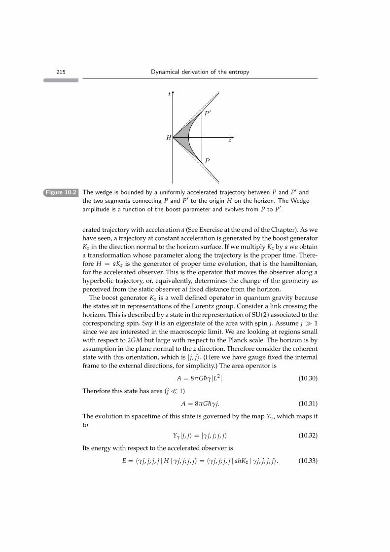
215 Dynamical derivation of the entropy
P
P
z
t
H
tFigure 10.2 The wedge is bounded by a uniformly accelerated trajectory between P and P′ and
the two segments connecting P and P′ to the origin H on the horizon. The Wedge
amplitude is a function of the boost parameter and evolves from P to P′.
erated trajectory with acceleration a (See Exercise at the end of the Chapter). As wehave seen, a trajectory at constant acceleration is generated by the boost generatorKz in the direction normal to the horizon surface. If we multiply Kz by a we obtaina transformation whose parameter along the trajectory is the proper time. There-fore H = aKz is the generator of proper time evolution, that is the hamiltonian,for the accelerated observer. This is the operator that moves the observer along ahyperbolic trajectory, or, equivalently, determines the change of the geometry asperceived from the static observer at fixed distance from the horizon.
The boost generator Kz is a well defined operator in quantum gravity becausethe states sit in representations of the Lorentz group. Consider a link crossing thehorizon. This is described by a state in the representation of SU(2) associated to thecorresponding spin. Say it is an eigenstate of the area with spin j. Assume j 1since we are interested in the macroscopic limit. We are looking at regions smallwith respect to 2GM but large with respect to the Planck scale. The horizon is byassumption in the plane normal to the z direction. Therefore consider the coherentstate with this orientation, which is |j, j〉. (Here we have gauge fixed the internalframe to the external directions, for simplicity.) The area operator is
A = 8πGhγ|L2|. (10.30)
Therefore this state has area (j 1)
A = 8πGhγj. (10.31)
The evolution in spacetime of this state is governed by the map Yγ, which maps itto
Yγ|j, j〉 = |γj, j; j, j〉 (10.32)
Its energy with respect to the accelerated observer is
E = 〈γj, j; j, j |H | γj, j; j, j〉 = 〈γj, j; j, j | ahKz | γj, j; j, j〉. (10.33)

216 Black holes
But since we are in a γ-simple representation, this is
E = 〈γj, j; j, j | ahγLz | γj, j; j, j〉 = a hγ j (10.34)
This can be rewritten in the form
E = ahγA
8πGhγ=
aA8πG
, (10.35)
Which is precisely the Frodden-Ghosh-Perez energy.This result, obtained by Eugenio Bianchi in [Bianchi (2012a)], is very remarkable.
To appreciate, observe that one need that Einstein equations to derive the Frodden-Ghosh-Perez relation. Here, the same relation emerges from the quantum theoryusing only the map Yγ and the SU(2) and SL(2,C) representation theory.
This confirms, indeed, that the information about the Einstein equations is en-coded in the Yγ map. Notice the manner in which the Barbero-Immirzi constantcancels.
The second main ingredient for deriving the Bekenstein-Hawking relation in thequantum theory is the observation that |γj, j; j, j〉 is a thermal state at temperatureT = h/2π for the flow generated by the operator Kz. This is shown by Bianchi inthe original paper [Bianchi (2012a)] by explicitly coupling a thermometer to thisstate, following the accelerated trajectory, and computing the ratio between upand down transitions among the thermometer states.
In fact, this is a general result for an accelerated observer in a Lorentz invariantcontext, as first realized by Unruh. To see this is, consider the wedge amplitude(7.62)
W(g, h) = ∑j(2j + 1) Trj[Y†
γ gYγh], (10.36)
which defines the dynamics of the theory. The amplitude for a transition betweenthe state |j, m〉 and the state |j, m′〉 as observed by an accelerated observer under-going a boost of Lorentzian angle η is given in (7.64)
Wj,m,m′(η) = 〈j, m′|Y†eiKηY|j, m′〉 (10.37)
together with its explicit form. The correlation function between an observable Aand an observable B respectively at the beginning and the end of this evolution is
GAB(η) = 〈W(η)|AB|Ψη〉, (10.38)
where Ψη is the boundary state. What is the boundary state representing a statewhich is locally Lorentz invariant? To answer this, consider a key property of theLorentz group: a boost rotates a spacelike vector into a spacelike vector and nevermoves a vector out of the wedge. But a boost with imaginary parameter is in facta rotation, and can move a vector across the light cone. In particular, a boost withimaginary parameter 2πi moves a vector around the Minkowski plane, and a boostwith imaginary parameter 2πi − η rotates the η half line to the η = 0 one. If we

217 Dynamical derivation of the entropy
take the boundary state to be given by the Lorentz dynamics outside the wedge,we can therefore postulate
Ψη = eiK(2π−η). (10.39)
' '+
eK
This is in fact nothing else than the quan-tum gravity version of the old formal ar-gument that gives an intuitive version ofthe Bisognano-Wichmann theorem [Bisog-nano and Wichmann (1976)] which givesthe mathematics underlying the Unruh ef-fect. The standard formal argument runsas follows. Consider a quantum field onMinkowski space. The vacuum state |0〉 canbe written as the path integral on the fieldsof the lower half plane.
〈ϕ|0〉 =∫
D[φ] eiS. (10.40)
If we split the field in its components ϕ± at the left and the right of the origin, ehave
〈ϕ−, ϕ+|0〉 =∫
D[φ] eiS. (10.41)
But his can be read as the evolution generated by a π rotation from the negative tothe positive x axis, thus
〈ϕ−, ϕ+|0〉 = 〈ϕ−|eπK|ϕ+〉 (10.42)
where K is the boost generator. If we now trace over ϕ− to get the density matrixrepresenting the statistical state restricted to the positive axis, we have
ρ = Trϕ− [〈ϕ−, ϕ+|0〉〈0|ϕ−, ϕ+〉] = Trϕ− [〈ϕ−|eπK|ϕ+〉〈ϕ+|eπK|ϕ−〉] = e2πK.(10.43)
Evolving this with with e−iKη to the boundary of the wedge we have the wedgeboundary state (10.39).
Bringing together the amplitude and the state, we have
GAB(η) = Tr[eiK(2π−η)BeiKη A] (10.44)
where the trace is taken in the unitary Lorentz representation. This correlationfunction satisfies the KMS property, which is the mark of a thermal configuration(see the Complements to this Chapter for a simple introduction to these notions),with dimensionless temperature
T =1
2π(10.45)
with respect to the dimensionless evolution parameter η. Scaling the evolution

218 Black holes
parameter to the proper time s = aη, where a is the acceleration of the observergives the Unruh temperature
TH =ha2π
. (10.46)
Above we have seen that the covariant dynamics gives the Frodden-Ghosh-Perezenergy. Here we have seen that it gives the Unruh temperature. The two together,as we have seen above, give the Bekenstein-Hawking entropy, with the correctfactor. This shows that the Bekenstein-Hawking entropy SBH can be derived en-tirely in the quantum theory. It also shows that it can be viewed as an effect of thequantum correlations across the horizon, because this is the source of the entropycaptured by the thermal state of the Bisognano-Wichmann theorem.
The calculation can be summarized as follows. The quantum state of spacetimenear the horizon has a form that is compatible with local Lorentz invariance. If werestrict it to the algebra of observables of an observer that keeps herself outsidethe hole, this is represented by the state
ρ = e−2πK (10.47)
where K is the generator of boosts normal to the horizon. This state has an entropy
S = −Tr[ρ log ρ]. (10.48)
Now suppose this state is modified by an arbitrary process that changes it by anamount δρ. Then the change in entropy is
δS = −δTr[ρ log ρ] = −Tr[(δρ) log ρ]− δTr[ρ1ρ
δρ]. (10.49)
The second term vanishes because ρ must remain normalized in the change. Thefirst term, using (10.47) and the relation between the boost generator and the Areaderived above gives
δS = Tr[(δρ)2πK] = 2πTr[(δρ)A
8πGh] = 2π
δA8πGh
=δA
4πGh= δSBH . (10.50)
So we find the (differential form of the) Bekenstein-Hawking relation.Say for simplicity we consider a local change of state given by a change δj in the
spin of a link crossing the horizon. Then we have the change in the energy
δE = a hγ δj (10.51)
and the change in entropy
δS = δE/T =a hγ δjha/2π
= 2πγδj. (10.52)
Thus up to a possible additive constant, the entropy associated to a link is a simplefunction of the spin
S = 2πγj (10.53)

219 Dynamical derivation of the entropy
and since the area of a link is A = 8πγGhj, this gives
S =2πγA8πγGh
=A
4hG(10.54)
again the Bekenstein-Hawking formula.
10.4.1 Entanglement entropy and area fluctuations
The two previous sections seem to point to different physical interpretations forthe origin of the black hole entropy. The first is the idea that this is the effect of thequantum fluctuations of the horizon. The second points to the idea that the blackhole entropy is given by the entanglement entropy across the horizon. Is there acontradiction?
No. The two interpretations are not in contradiction with one another; they aretwo faces of the same phenomenon, the local quantum fluctuations (of anything)near the horizon. On the one hand, these fluctuations generate geometry fluctua-tions, and therefore can be visualized as a quantum “shaking” of the horizon, ora Planck scale “thickness” of the horizon, due to the fact that this cannot be re-solved at a scale smaller than the Planck scale. On the other hand, we can hold amental picture where the horizon is fixed in some (imaginary) background coordi-nates, and the quantum field theoretical fluctuations have finite wavelengths thatcorrelate the value of any field across the horizon.
For some time the possibility that the black hole entropy be related to entangle-ment entropy across the horizon has been considered implausible because of anobvious objection: the horizon fluctuations are a purely geometrical phenomenonand therefore can justify a universal formula like the Bekenstein-Hawking for-mula. But the horizon entanglement is a feature of all quantum fields that arepresent, and therefore the entropy should increase if the number of fields increase.Why then the Bekenstein-Hawking formula does not depend on the number offields? The solution to this puzzle has recently been found by Eugenio Bianchi[Bianchi (2012b)], who has computed the variation of the entanglement entropySent and of the horizon area A in a physical process, using standard quantum fieldtheory and classical general relativity. He has found that these variation are finiteand given by
δSent =δA
4hG, (10.55)
independently from the cut off and from the number of fields. The key to the mys-tery is that δSent does not increase with the number of fields, because at smallscale the fields are not independent. The cut off on the fields modes goes into ef-fect when the total energy density of the fields reaches the Planck scale. The totalenergy density depends on the individual field’s fluctuations plus their (negative)potential gravitational energy. Therefore he cut off scale on the wavelength of anindividual field depends on the presence of other fields, which are fluctuating atsmall scale as well. Alltogether, the result is that the entanglement entropy does

220 Black holes
not dependent on he number of fields. (On this, see also the intriguing recent re-sults in [Ghosh et al. (2013)] and [Frodden et al. (2012); Han (2014)].)
The issue of understanding black-hole entropy directly in quantum gravity hasbeen largely clarified by these loop gravity results. The entropy of a black hole isa local phenomenon due to the fact that stationary observers are accelerating. It isrelated to quantum fluctuations of the horizon or, equivalently, to entanglementacross the horizon. The entropy can be computed from first principles, includ-ing the famous 1/4 Hawking factor, it is finite and the calculation can be donefor realistic black holes, such as a Schwartzschild or Kerr hole. This is beautifulachievement of the theory which for the moment is not matched by any of theother tentative quantum theories of gravity.
10.5 Complements
10.5.1 Accelerated observers in Minkowski and Schwarzshild
Exercise: Consider a uniformly accelerated particle in Minkowski space, following the tra-jectory
t = l sinh η, (10.56)x = l cosh η. (10.57)
show that the acceleration is constant and is a = 1/l, the proper time among the trajectoryis s = ηl, the distance between the particle and the origin is constant and given by l, the nullline x = t is a horizon for this particle, and no signal emitted at t = 0, x < 0 can reach theparticle. What is the Unruh temperature felt by this particle?
Exercise: Consider a uniformly accelerated particle in Schwarzshild spacetime, followingthe trajectory
r = 2GM + ε. (10.58)
where ε 2GM. Show that show that the acceleration is a = 1/l where l is the physicaldistance of the particle from the horizon. Show that this distance is constant (do not confuseit with ε)! Compute the temperature felt by this particle using the Hawking temperature atinfinity and the Tolman law. Compare with the previous exercise.
10.5.2 Tolman law and thermal time
If we ignore general relativity, two systems are in equilibrium when they have the sametemperature. An isolated column of gas in a (Newtonian) gravitational field, for instance,will thermalise to an equilibrium state where the pressure decreases with altitude by thetemperature is constant. This, however, is no longer true when general relativity is taken

221 Complements
into account. At equilibrium, the temperature T (measured by a standard thermometer) ofthe gas will decrease with the altitude as
∆TT
=gc2 (10.59)
where g ∼ 9.8m/s2 is Galileo acceleration. The covariant version of this relation is
T ||ξ|| = constant, (10.60)
where ||ξ|| is the norm of the Killing field ξ along which equilibrium established. This fact,which at first is quite surprising was first derived theoretically by Tolman and Ehrenfestin the early thirties [Tolman (1930); Tolman and Ehrenfest (1930)], and then re-derived in anumber of ways by many authors.
The simplest way to understand it is simply to observe that gravity slows down time.In a stationary gravitational field, stationary clocks do not remain synchronised. Thereforethere are two distinct notions of time flow, in a stationary field: the common time τ givenby the Killing field, along which spacetime is stationary, and the local time s, given by theproper time along each trajectory at rest. The ratio of the two is given by the norm of theKilling field. A clock is a devise that measures the transition probability between energylevels, and these levels are determined by the proper time, not by τ. But an equilibriumconfiguration is in equilibrium with respect to the flow of the Killing field, namely in τ, notin s. Therefore the different regions in a global equilibrium configuration are red-shiftedwith respect to the other, by the ratio between τ and s.
Another way if viewing the same effect is to realise that in general relativity energy”weight”, and therefore accumulates at lower altitude. More precisely, when energy leavesa lower part of the system and reaches a hight part of it, it arrives red shifted, thereforediminished. It follows that we cannot anymore maximise entropy by assuming that the en-ergy lost by one subsystem is gained by the other: we must include the red shift factor inthe calculation, and this gives (10.59)
The equilibrium time parameter τ is an example of thermal time [Rovelli (1993a); Connesand Rovelli (1994)]. Temperature can be defined by the ratio between the thermal time andthe proper time T ∼ dτ/ds. The proportionality factor fixes the scale of the Killing field andthermal time [Rovelli and Smerlak (2010)]. Fixing it to
T =hk
dτ
ds(10.61)
is particularly convenient because it makes τ dimensionless and it identifies it with thenumber of individual quantum cells jumped over by a system at equilibrium: see [Haggardand Rovelli (2013)].
10.5.3 Algebraic quantum theory
We describe here the basic formalism of thermal states in the algebraic language, used inthe text. This is more general and more powerful than the standard Hamiltonian languagefor describing thermal states.
We also give a direct physical interpretation of the KMS condition, in terms of thermome-ter coupling.
Consider a quantum system with Hilbert space of statesH, hamiltonian H and an algebraA of self-adjoint observables A, B.... Every state ψ ∈ H defines a positive linear function onthe algebra by
ωψ(A) = 〈ψ|A|ψ〉 (10.62)
and so does, more in general, any density matrix ρ
ωρ(A) = Tr[ρA]. (10.63)

222 Black holes
The hamiltonian defines a flow on the algebra by
αt(A) = eiHt Ae−iHt. (10.64)
The algebra A with the flow αt and the set of its positive state ω provides a language fortalking about quantum theory which is more general than the Hilbert space one (see below).Let us use this language to describe thermally.
10.5.4 KMS and thermometers
Consider a quantum system described by an observable algebraA, with observables A, B, ...,which is in a state ω : A → C. Let αt : A → A with t ∈ R be a flow on the algebra. We saythat the state ω is an equilibrium state with respect to αt if for all t,
ω(αt A) = ω(A), (10.65)
and that its temperature is T = 1/β if
fAB(t) = fBA(−t + iβ) (10.66)
where
fAB(t) = ω(αt A B). (10.67)
An equivalent form of (10.66) is given in term of the Fourier transform fAB of fAB as
fAB(ω) = e−βω fAB(−ω). (10.68)
The canonical example is provided by the case where A is realized by operators on aHilbert space H where a Hamiltonian operator H with eigenstates |n〉 and eigenvalues Enis defined, the flow and the state are defined in terms the evolution operator U(t) = e−iHt
and the density matrix ρ = e−βH = ∑n e−βEn |n〉〈n|, by
αt(A) = U−1(t)AU(t) (10.69)
and
ω(A) = tr[ρA] (10.70)
respectively. In this case, it is straightforward to verify that equation (10.65) and (10.66)follow.
However, the scope of equations (10.65) and (10.66) is wider than this canonical case. Forinstance, these equation permit the treatment of thermal quantum field theory, where theHamiltonian is ill-defined, because of the infinite energy of a thermal state in an infinitespace. It is indeed important to remark that these two equations capture immediately thephysical notions of equilibrium and temperature. For equation (10.65), this is pretty obvi-ous: the state is in equilibrium with respect to a flow of time if the expectation value of anyobservable is time independent.
The direct physical interpretation of equation (10.66) is less evident: it describes the cou-pling of the system with a thermometer.
To see this, consider a simple thermometer formed by a two-state system with an energygap ε, coupled a quantum system S by the interaction term
V = g(|0〉〈1|+ |1〉〈0|)A. (10.71)
where g is a small coupling constant. The amplitude for the thermometer to jump up from

223 Complements
the initial state |0〉 to the final state |1〉, while the system moves from an initial state |i〉 to afinal state | f 〉 can be computed using Fermi golden rule to first order in g:
W+(t) = g∫ t
−∞dt (〈1| ⊗ 〈 f |) αt(V) (|0〉+ |i〉)
= g∫ t
−∞dt eitε〈 f |αt(A)|i〉. (10.72)
The probability for the thermometer to jump up is the modulus square of the amplitude,summed over the final state. This is
P+(t) = g2∫ t
−∞dt1
∫ t
−∞dt2 eiε(t1−t2)ω(αt2 (A†)αt1 (A))
where we have used the algebraic notation ω(A) = 〈i|A|i〉. If the initial state is an equilib-rium state
P+(t) = g2∫ t
−∞dt1
∫ t
−∞dt2 eiε(t1−t2) fA†A(t1 − t2).
and the integrand depends only of the difference of the times. The transition probabilityper unit time is then
p+ =dP+dt
= g2 fA†A(ε) (10.73)
which shows that (10.67) is precisely the quantity giving the transition rate for a thermome-ter coupled to the system. It is immediate to repeat the calculation for the probability tojump down, which gives
p− = g2 fAA† (−ε). (10.74)
And therefore (10.68) expresses precisely the fact that the thermometer thermalizes o attemperature β, that is p+/p− = e−βε
These observations show that equations (10.65) and (10.66) define a generalization ofthe standard quantum statistical mechanics, which fully captures thermal properties of aquantum system. The structure defined by these equations is called a modular flow in themathematical literature: αt is a modular flow, or a Tomita flow, for the state ω, and is thebasic tool for the classification of the C∗ algebras. In the physical literature, the state ω iscalled a KMS state (for the time flow). In order to show that a system is in equilibrium andbehave thermally in a certain state, it is sufficient to show that the state satisfies these twoequations.
Notice that in the context of Hilbert space quantum mechanics, a state can satisfy thesetwo equations also if it is a pure state. The standard example is provided by the vacuumstate of a Poincare invariant quantum field theory, which is KMS with respect to the mod-ular flow defined by the boost in a given direction. Being Poincare invariant, the vacuumis invariant under this flow, and a celebrated calculation by Unruh shows that it is KMS atinverse temperature 2π.
In this case, the physical interpretation is simply given by the fact that an observer sta-tionary with respect this flow, namely an accelerated observer at unit acceleration, will mea-sure a temperature 1/2π. Unruh’s original calculation, indeed, follows precisely the stepsabove in equations (10.71-10.74).
10.5.5 General covariant statistical mechanics and quantumgravity
The relations between gravity, quantum and statistics form a net of intertwined problems,where much of our confusion on the fundamental aspects of nature lies. At the core of the

224 Black holes
difficulty is the fact that we lack a coherent statistical theory for the gravitational field (as wehave one for the electromagnetic field), even in the classical case. The reason is related to thepeculiar manner time appears in general relativity, which makes the standard tools of statis-tical mechanics useless. The effort of extending the power of statistical reasoning to generalcovariant theories is, in our opinion, among the deepest and most beautiful problems openat the core of our present understanding of the physical world. As beautiful as, and mostlikely strictly related to, quantum gravity. Here we only sketch briefly a few results andideas in a research line in this direction under development by the authors, pointing to therelevant literature.
Thermal time in the classical theory. If all the variables are on the same footing, it is notclear what equilibrium means. In such a situation (generically) any statistical stateρ can be seen as an equilibrium state, because it is invariant under a flow in phasespace: the hamiltonian flow generated by H = − ln ρ. Since ρ is a density on phasespace, it has the dimension of inverse action, therefore we need a constant to fix itslogarithm. Looking ahead, we do so by taking h=1 units. The quantity H is calledthe thermal hamiltonian of the state ρ and the (dimensionless) flow parameter τis called thermal time [Rovelli (1993a)]. The thermal hamiltonian of a Gibbs stateis the standard hamiltonian scaled by the temperature and the temperature is theratio between the thermal time τ and the physical time t:
T =hk
τ
t, (10.75)
an expression we have already seen in (10.61) generalises to gravity, where t be-comes the proper time s which varies, as does the temperature, from point to point.
Mean geometry. If we study the thermal fluctuations of the gravitational field, then it isreasonable to call “equilibrium” a state where the these fluctuations are centredaround a “mean geometry” having a Killing field which can be identified with thethermal time flow. This construction is developed in [Rovelli (2013a)].
Thermal time in quantum field theory. The idea of thermal time gets bite in quantum fieldtheory, where the thermal time flow is the modular flow of the state, which isindependent on the state up to unitaries [Connes and Rovelli (1994)]. The modularflow of the vacuum state of a quantum field theory, restricted to the algebra of theobservables on the Rindler wedge x> |t|, is the flow of the boost, the thermal timeis the boost parameter and the local temperature defined by (10.75) is the Unruhtemperature. But the thermal flow makes sense also in non stationary situations,like for instance a Friedmann cosmology, where the thermal time of the cosmicbackground radiation state turns out to be the cosmological time [Rovelli (1993c)].
The zero’th principle. Remarkably, when two systems interact, equilibrium is given by theequality of their thermal times [Haggard and Rovelli (2013)]. This has a physicalinterpretation: thermal time is time in the units given by the time a quantum statemoves to a state orthogonal to itself. Therefore two interacting systems in equilib-rium interact with the same number of distinct states: the net flux of informationthey exchange vanishes. This notion of equilibrium, defined in terms of informa-tion rather than in term of a preferred time variable, generalises to the covariantsystems where no preferred time is available [Haggard and Rovelli (2013)]. In turn,the combined state of the two systems itself can select a time variable among thecombination of the individual times [Chirco et al. (2013)].
Statistical states in the boundary formalism. In Section 2.4.2 we have argued that in grav-ity we need to associate states to the full boundary Σ of a spacetime region. If Σcan be split into a past and a future component, this Hilbert space has the structureH = Hpast ⊗H f uture. This space contains states that are not of the tensor productof a state inHpast and a state inH f uture. What do these represent? It is not difficultto see that they represent statistical states [Bianchi et al. (2013)].
.

225 Complements
tFigure 10.3 Lens shaped spacetime region with spacelike boundaries and corners (filled circles).
Statistical versus quantum fluctuations. In particular, if there is a corner joining the fu-ture and the past components of the boundary, as in Figure 10.3 and if a quantumversion of the equivalent principle holds, implying that the corner is locally likea Minkowski state in the UV, then it follows that all boundary states are mixes.Because locally in the corner the state has the form
ρ = e−2πK (10.76)
where K is the boost generator at the corner. This supports the idea that statisticalfluctuations and thermal fluctuations become indistinguishable when gravity andhorizons are in play.
These brief notes are of course far from exhausting this fascinating topic, which still seek-ing for clarity.

11 Cosmology
The major application of loop gravity to a realistic physical phenomenon is earlycosmology. This is also the most important application, because it appears to bethe most likely to lead to predictions that could confirm the theory. Observationalcosmology is advancing rapidly and there is hope that loop gravity could leadto specific testable predictions in cosmological observations, in particular in thecosmic background radiation.
As for the case of black hole thermodynamics, there are two main avenues forapplying loop gravity to cosmology. The first is based on the canonical formulationof the theory, the second on the covariant formulation. Both are based on the sameidea as classical relativistic cosmology: focusing on the dynamics of the very largescale degrees of the universe [Einstein (1917)]. Here we touch on the first onlybriefly, and we discuss a bit more in detail the second. We begin by reviewing theclassical formulation of a simple cosmological model, concentrating on the aspectsrelevant for the quantum theory.
11.1 Classical cosmology
Cosmology is not the study of the totality of the things in the universe. It is thestudy of a few very large-scale degrees of freedom. It is a fact (intuited by Einstein)that at very large scale the universe appears to be approximately homogenous andisotropic. Therefore it admits an approximate description obtained expanding inmodes around homogenous-isotropic geometries.
The spatial curvature of the universe appears to be very small at the scale weaccess. One must not conclude from this observation that the universe is spatiallyflat: humanity has already made this mistake once: the Earth’s average curvatureis very small at our scales and we concluded that the Earth is flat. Let us not repeatthis mistake (many do). But to a good approximation a spatially flat universe ap-proximates the patch of the Universe that we see, and since a spatially flat universeis a bit easier to describe than a closed one, at least for some purposes, it makessense to use a spatially flat metric here.
Thus, consider a Friedman-Lemaıtre metric, where the function a(t) is the scalefactor, and write it in terms of tetrads:
ds2 = −N(t)dt2 + a(t)2d~x2 = ηI J eIµ(t) eJ
ν(t) dxµdxν (11.1)
where, introducing eIµdxµ = eI ,
226

227 Classical cosmology
e0 = N(t)dt ei = a(t)dxi . (11.2)
Inserting this metric into the action gives
S[a] =3
16πG
∫dt N
(a2a− Λ
3a3)+ Smatter (11.3)
The momentum conjugate to the scale factor is
pa =∂L∂a
=3Vo
8πGNaa (11.4)
where L is the Lagrangian and Vo is the coordinate volume of the space considered.This volume cannot be taken infinite without introducing a confusing infinite inthe formalism. So we take it finite. Normalizing the coordinates so that Vo = 1 hasthe consequence that a3 is the actual volume of the universe. With this choice, theboundary term in the gravitational action is then
Sboundary = paa =3
8πGNaa2. (11.5)
The dynamics of the scale factor defines a one-dimensional dynamical system,which is the ground for studying physical cosmology. Solution to this system andperturbations around these solutions describe the large scale dynamics of the uni-verse quite well. The recent observations by the Planck satellite [Planck Collabo-ration (2013)] have confirmed the credibility of this picture to a surprising degreeof accuracy.
The equation of motion obtained varying the Lapse function N is an equationthat ties a and a. In the presence of a matter energy density
ρ(t) = a3 ∂Smatter
∂N(t)(11.6)
the variation of the Lapse gives(
aa
)2=
Λ3+
83
πGρ, (11.7)
which is the Friedmann equation, the main equation governing the large scaledynamics of the universe. After taking this equation into account, we can fix theLapse, say at N = 1. The Friedman equation gives a as a function of a at every time.Therefore we can view the boundary term simply as a function of a. It follows thatthe Hamilton function is a pure boundary term of the form
S(ai, a f ) = S(a f )− S(ai) (11.8)
where
S(a) =3
8πGaa2 (11.9)
and a depends on a via the Friedmann equation. Therefore we must expect thetransition amplitude of the quantum theory in the small h limit to factorize
W(ai, a f ) ∼ eih S(ai ,a f ) = e
ih S(a f )− i
h S(ai) = eih S(a f )e−
ih S(ai) ∼W(a f )W(ai) (11.10)

228 Cosmology
where
W(a) ∼ e−ih aa2
. (11.11)
This is the classical limit to which a cosmological quantum transition amplitudemust converge, if it is has to agree with standard cosmology.
Let us translate this to the Ashtekar variables defined in Section 3.4.3 . TheAshtekar-Barbero connection Ai
a = Γia + γ ki
a conjugate to the densitized inversetriad Ea
i = 12 εabcεijkej
bekc is the sum of the spin-connection Γi
a of the triad and theextrinsic curvature of the spacial slide ki
a multiplied by the Barbero-Immirzi con-stant β, that we here take equal to γ, as usual in loop quantum cosmology. In theflat case Γi
a = 0 because space is flat and the extrinsic curvature is diagonal and amultiple of the time derivative of the scale factor
kia = ei
a = aδia. (11.12)
Therefore the Ashtekar-Barbero variables are reduced to
Aia = γ a δi
a = cδia Ea
i = a2δai = pδa
i , (11.13)
which satisfy
c, p = 8πG3Vo
γ. (11.14)
Inserting these variables in the hamiltonian constraint (3.86) gives (up to an irrel-evant overall constant)
H =
(cpγ
)2− Λ
3p3. (11.15)
H = 0 is the Friedmann equation for pure gravity. Adding the matter energydensity ρ (assumed constant in space) we obtain
c2
γ2 p=
Λ3+
83
πGρ, (11.16)
which translated back into the a(t) variable is (11.7), namely the standard Fried-mann equation for a flat universe with cosmological constant. The Hamilton func-tion factorizes as above and reads
S(p) ∼ c(p)pγ
(11.17)
where c(p) is the solution of the Friedmann equation. Notice that γ cancels. Forinstance, if there is no matter, we expect
S(p) ∼√
Λ3
p32 . (11.18)
Thus for the classical limit to hold, the transition amplitude must have the small hbehavior
W(p) ∼ eih
√Λ3 p
32
. (11.19)

229 Canonical Loop Quantum Cosmology
11.2 Canonical Loop Quantum Cosmology
A large body of work has been developed to study the canonical quantization ofthe dynamical system defined by the dynamics of the scale factor, as well as theperturbations around it. We refer the interested reader to recent reviews, such as[Ashtekar and Singh (2011)] and [Bojowald (2011)], which follow slightly differentpaths, and references therein.
The main result of this work is that the dynamics of the quantum dynamical sys-tem describing the evolution of the scale factor is well-defined also around whatappears in the classical approximation as the initial singularity. That is, the BigBang singularity does not appear to be a physical event, but only an artifact of theclassical approximation. In this, it is analogous to the possibility for an electron tofall into the nucleus of the atom, which is predicted by the classical approxima-tion but not by the quantum theory of the electron. The quantum evolution of theuniverse near the Big Bang is well defined, and no singularity develops.
Interestingly, the quantum corrections can be approximated in terms of a modi-fied classical dynamical evolution for a wave packet. This gives a modified Fried-man equation. In the case Λ = 0 and k = 0, for instance, one obtain
(aa
)2=
8πG3
ρ
(1− ρ
ρc
), (11.20)
where the critical density ρc is a constant with a value that is approximatetivelyhalf of the Planck density (ρPl ≈ 5.1× 1096kg/m3). In the absence of the correctionterm, a cannot change sign at small scales. In the presence of the correction term, acan vanish, and the dynamics of the scale factor “bounces”: semiclassical trajecto-ries describe a collapsing universe that bounces into an expanding one. We do notgive a derivation of (11.20) here, see [Ashtekar and Singh (2011)], but a few wordson how this happens may be useful.
The idea is to study a quantum system with Friedman cosmology as classicallimit using two key inputs from the full theory.
i.) The first is the idea that the proper operators are not the local ones but the in-tegrated ones. In particular, the relevant operator is not the connection butrather its holonomy. This translates into cosmology in the request that the op-erator well defined in the quantum theory is not c but rather eiµc, for suitableµ.
ii.) The second is that the dynamics is modified to take into account the quantumdiscreteness of space. This is obtained by replacing the curvature in the hamil-tonian constraint with the holonomy around a small circuit encircling thesmallest possible quantum of area.
The first input allows the definition of a suitable Hilbert space where the operatorseiµc are defined. The second permits the definition of the dynamics. A detailedanalysis of the resulting system and its semiclassical limit yields then the above

230 Cosmology
result. The resolution of cosmological singularities can be seen to be quite generic[Singh (2009); Singh and Vidotto (2011)].
The Poisson brackets (11.14) become commutators in the quantum theory, andyield Heisenberg uncertainty relations
∆c∆p >8πhG3Vo
γ. (11.21)
By taking Vo arbitrarily large, the uncertainties can be made arbitrarily small. Thisis analogous to the fact that by taking an object made by sufficiently many atomswe can have its position and velocity arbitrarily well defined. In other words, loopquantum cosmology looks only at the large modes of the field, which are averagesin space of the gravitational field, and is blind to the local quantum fluctuationof the gravitational field, which are dominated by shorter wavelength modes. Itfollows that the theory, so far, does not describe the actual fluctuating geometry athe bounce. The bounce is not determined by the universe being small, but by thematter energy density reaching Planck scale, and this can happen, depending onthe matter content of the universe, at any size of the universe.
We also report here, without deriving it, the effect of quantum gravity on cos-mological perturbations. Remarkably this as well can be summarized in a correc-tion to the standard cosmological perturbation theory. The Mukanov equation thatgoverns the dynamics of the perturbations [Mukhanov et al. (1992)]
v−∇2v− zz
v = 0, (11.22)
is corrected to [Cailleteau et al. (2012a,b)]
v−(
1− 2ρ
ρc
)∇2v− z
zv = 0. (11.23)
An electron does not fall into the Coulomb potential because of the uncertaintyprinciple, which forbids concentrating it into too small a region of space withouthaving a large momentum that allows it to escape. In a sense, quantum mechanicsprovides an effective repulsive force at short distance. The same happens for theuniverse: when too much energy density is concentrated into too small a region,the uncertainty principle prevents further collapse and acts as an effective strongrepulsive force.
The precise interpretation of this semiclassical bounce is in our opinion notcompletely clear yet, because more understanding of the quantum fluctuations ofspacetime at the bounce is needed. The full physics of the gravitational field nearthe bounce is not yet well understood. Is spacetime still approximately classical atthe bounce or do the full quantum fluctuations make the very notion of spacetimeill defined around the bounce, as the notion of a classical trajectory is ill definedfor an electron falling into a Coulomb potential? In the second case, the picture ofa “previous” contracting phase of the universe bouncing into a “later” expandingone might be naive for some purposes: spacetime itself becomes ill defined in earlycosmology.

231 Spinfoam Cosmology
s ttFigure 11.1 Two tetrahedra, glued by all their faces, triangulate a 3-sphere.
11.3 Spinfoam Cosmology
The approach to quantum cosmology based on the covariant formulation of loopgravity was introduced in [Bianchi et al. (2010e)] and is called “spinfoam cosmol-ogy”. The expansion at the basis of the covariant theory is suitable for cosmology,because it is an expansion in the number of degrees of freedom. Since a cosmo-logical model is the reduction of general relativity to a small number of degrees offreedom, it can be naturally described at low order in the spinfoam expansion.
Consider a closed homogeneous and isotropic universe, with the spacial geom-etry of a 3-sphere S3 of radius a, evolving in time. We want to study the quantumdynamics of the degree of freedom a(t) as well as the quantum dynamics of thelarge-scale deformations of the three sphere.
In a finite lapse of time, a compact universe evolves from a 3-sphere to a 3-sphere. Therefore we want the transition amplitude form a state of quantum spacewith the topology of a 3-sphere to different quantum state of space with the topol-ogy of a 3-sphere. To represent one such states, we have to choose a discretisationof a 3-sphere. Spinfoam cosmology was first studied using the simplest cellulardecomposition of S3. This can be obtained by gluing two tetrahedra by all theirfaces.1 The graph dual to this triangulation of S3 is obtained by placing a nodeon each tetrahedron and connecting the two nodes accords each of the four faces.(Figure 11.1). This graph is called Γ2, or “dipole graph”: it is formed by 2 nodes
1 The common sphere S2 can be obtained by taking two triangles and gluing them by their sides.
tFigure 11.2 Five tetrahedra triangulate a 3-sphere.

232 Cosmology
connected by 4 links. Quantum cosmology on this graph was first studied in thehamiltonian language [Rovelli and Vidotto (2008); Battisti et al. (2010); Borja et al.(2010, 2011)]. More general regular graphs were studied in [Vidotto (2011)]. Forinstance, we can obtain a three sphere by pairwise gluing five tetrahedra, as inthe boundary of a four-simplex (Figure 11.2).2 In the following we use a genericregular graph Γ. The first step to describe the large scale geometry of the universeis to write the boundary states in the Hilbert space HΓ, representing semiclassicalconfigurations. Then we can take a couple of these states, which can be thought ofas in and out states, and compute the corresponding transition amplitude.
11.3.1 Homogeneus and isotropic geometry
Fix a regular graph, namely a graph where all the nodes have the same numberof links.3 As an example, we can think about Γ5, the graph formed by five nodesall connected. Pick a cellular decomposition of a (metric) three sphere formed byequal cells and dual to the regular graph. Approximate each cell with a flat cellhaving the same volume, face area and average area normal. This defines normals~nl associated to each oriented link of the graph. By regularity, all areas and ex-trinsic curvatures on the graph are equal. We can construct a coherent state on thegraph, based on these geometrical data, using the coherent states developed inSection 8.4. The coherent state is determined by an SL(2, C) element H` for eachlink, where H` is determined by the two (distinct) normals associated to two cellsbounding the face, and a complex number z, which is the same for all links. Thereal and imaginary parts of z are determined by the area and the extrinsic curva-ture on the face. We assume on the basis of (8.120), that the relation between theseand the coefficients of an isotropic geometry are given simply by
z = c + itpl2o
(11.24)
(For a finer analysis, see [Magliaro et al. (2011)]). Notice that the Planck length inthe denominator is imposed by (8.120) as well as by dimensions.
Γ5
Let us now seek quantum states that describe thegeometry of these triangulated spaces. For this, con-sider the extrinsic coherent states ψH`
(h`) in theHilbert spaceHΓ introduced in Section 8.4. Recall thatthese are determined by the data (cl , pl , ns(l), nt(l))
With these assumptions, a homogeneous isotropiccoherent state on a regular graph is described by asingle complex variable z, whose imaginary part isproportional to the area of each regular face of the cellular decomposition (and
2 The common sphere S2 can be obtained by taking fours triangles and gluing them by their sides, asin the boundary of a tetrahedron.
3 There are an infinite number of such graphs. For instance, two nodes can be connected by arbitrarynumber of links. Examples of regular graphs with N > 2 are given by the (dual of) the Platonicsolids.

233 Spinfoam Cosmology
it can be put in correspondence with the total volume) and whose real part isrelated to the extrinsic curvature [Rovelli and Speziale (2010)]. We denote ψH`(z)this state, and ψH`(z,z′) = ψH`(z) ⊗ ψH`(z′) the state on two copies of the regulargraph, obtained by tensoring an “in” and a “out” homogeneous isotropic state.These states are peaked on an homogenous and isotropic geometry, but since theyare genuine coherent states, they include the quantum fluctuations around thisgeometry, for the degrees of freedom captured by the graph.
11.3.2 Vertex expansion
For a boundary state formed by two disconnected components, the transition am-plitude determines the probability to go from one state to the other. For the coher-ent states that have just been introduced, this reads
WC(z′, z) = 〈z′ |W | z〉 =∫
dh`∫
dh′` ψz′(h′`) WC(h′`, h`) ψz(h′`) (11.25)
The transition amplitude can be computed by approximating it with a truncatedversion of the theory, namely by choosing a two-complex C bounded by the bound-ary graph, that is by two Γ5 graphs. At the lowest order, we have have the contri-bution of a two-complex without vertices.
〈z′ |WCo | z〉 ∼ (11.26)
This vanishes if the initial and final states are sufficiently far apart, which is thenon-trivial case we are interested in. Let us therefore study the first-order term,determined by a two-complex with a single vertex
〈z′ |WC1 | z〉 ∼ s (11.27)
We write this transition amplitude using (7.67) and (7.68)
WC1(h′`, h`) = W(h′`)W(h`) (11.28)
where
W(h`) =∫
SL(2,C)dg′e
L
∏`=1
P(h`, ge) (11.29)

234 Cosmology
The integration over the SL(2, C) elements hn associated to the edges imposesLorentz invariance. It is over all the gn but one. Using these, and the definition(8.126) of the coherent states, a short calculation gives
WC1(z′, z) = W(z)W(z′) (11.30)
where
W(z) =∫
dh`∫
dg′nL
∏`=1
Kt(h`, H`(z)) P(gn, h`)
=∫
dg′nL
∏`=1
∑j`
(2j`+1) e−2tj`(j`+1) D(j`)mm′(H`(z)) D(γj`,j`)
jm′ jm (G`). (11.31)
The transition amplitude factorizes, as we expected from the classical theory. Eachindividual term W(z) can be interpreted as a Hartle-Hawking “wave function ofthe universe” determined by a no-boundary initial condition [Hartle and Hawking(1983)], namely the amplitude to go from nothing to a give state. The reason thisis equivalent to the transition amplitude from a given geometry to another is thereflection of the fact that in the classic theory the dynamics can be expressed as arelation between the scale factor and its momentum, which is a relation at a singletime. The probability of measuring a certain “out” coherent state does not dependon the “in” coherent state.
Let us now evaluate W(z) in the semiclassical regime
11.3.3 Large-spin expansion
We are interested in (11.31) in the regime where the volume of the 3-sphere (whichis determined by p) is large compared to the Planck scale. By (11.24), this corre-sponds to the regime where the imaginary part of z is large. From (8.129), we have
D(j)(H`(z)) = D(j)(R~ns) D(j)(e−iz σ32 ) D(j)(R−1
~nn). (11.32)
When the imaginary part of z is large, Im z 1, the Wigner matrix
D(j)(e−iz σ32 ) = ∑
me−izm |m〉〈m| . (11.33)
is dominated by the term m = j, therefore
D(j)(e−iz σ32 ) ≈ e−izj |j〉〈j|, (11.34)
where |j〉 is the eigenstate of L3 with maximum eigenvalue m = j in the represen-tation j. Inserting this into (11.32) gives
D(j)(H`(z)) = D(j)(R~ns) |j〉 e−izj 〈j|D(j)(R−1~nn
). (11.35)
and recalling the definition (8.23) of the intrinsic coherent states this is
D(j)(H`(z)) = e−izj | j,~n` 〉〈 j,~n` | . (11.36)
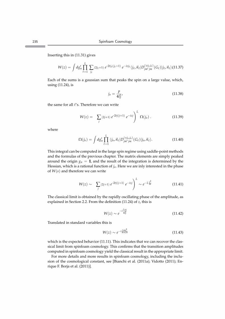
235 Spinfoam Cosmology
Inserting this in (11.31) gives
W(z) =∫
dg′nL
∏`=1
∑j`
(2j`+1) e−2tj`(j`+1) e−izj`〈j`,~n`|D(γj`,j`)jm′ jm (G`)|j`,~n`〉.(11.37)
Each of the sums is a gaussian sum that peaks the spin on a large value, which,using (11.24), is
jo =p
4l2o
, (11.38)
the same for all `’s. Therefore we can write
W(z) =
(∑
j(2j+1) e−2tj(j+1) e−izj
)L
Ω(jo) . (11.39)
where
Ω(jo) =∫
dg′nL
∏`=1〈jo,~n`|D(γjo ,jo)
jm′ jm (G`)|jo,~n`〉. (11.40)
This integral can be computed in the large spin regime using saddle-point methodsand the formulas of the previous chapter. The matrix elements are simply peakedaround the origin gn = 1l, and the result of the integration is determined by theHessian, which is a rational function of jo. Here we are inly interested in the phaseof W(s) and therefore we can write
W(z) ∼(
∑j
(2j+1) e−2tj(j+1) e−izj
)L
∼ e−L z28t (11.41)
The classical limit is obtained by the rapidly oscillating phase of the amplitude, asexplained in Section 2.2. From the definition (11.24) of z, this is
W(z) ∼ e−i Lcq
4l2o (11.42)
Translated in standard variables this is
W(z) ∼ e−i Laa28πGh (11.43)
which is the expected behavior (11.11). This indicates that we can recover the clas-sical limit from spinfoam cosmology. This confirms that the transition amplitudescomputed in spinfoam cosmology yield the classical result in the appropriate limit.
For more details and more results in spinfoam cosmology, including the inclu-sion of the cosmological constant, see [Bianchi et al. (2011a); Vidotto (2011); En-rique F. Borja et al. (2011)].

236 Cosmology
11.4 Maximal acceleration
Spinfoam cosmology is not yet developed to the point of allowing us to describethe quantum physics of the near-black-hole region directly. However, it does pro-vide an indirect element of evidence for the resolution of the classical singularity,because it directly predicts a limit on the acceleration. The idea that quantum grav-ity may limit the acceleration is old [Caianiello (1981); Caianiello and Landi (1985);Brandt (1989); Toller (2003)]. In covariant loop quantum gravity, it can be seen as adirect consequence of the quantisation of the area and the simplicity relations thatrelate area and boost [Rovelli and Vidotto (2013)]. To see this, consider a uniformlyaccelerated observer in Minkowski space, with acceleration a. The wedge definedby a portion of its trajectory is depicted in Figure (10.2). Specifically, taking theboost angle of this wedge η = 1, it is an easy calculation to see that the Lorentzianarea of the wedge is
Al =1
2a2 (11.44)
Therefore the Area of this wedge measures the acceleration of the observer. Butin turn, the Lorentzian area of this wedge is tied to the Euclidean area Ae by thelinear simplicity constraint
Al =1γ
Ae (11.45)
and since the minimum non vanishing eigenvalue of Ae is 8πGhγ√
1/2(1/2 + 1),it follows that the maximal value of the acceleration is
amax =
√1
8πGh. (11.46)
In turn, a maximal acceleration screens the classical singularity. The resolutionof classical singularities under the assumption of a maximal acceleration has beenstudied using canonical methods for Rindler [Caianiello et al. (1990)], Schwarzschild[Feoli et al. (1999)], Reissner-Nordstrom [Bozza et al. (2000)], Kerr-Newman [Bozzaet al. (2001)] and Friedman-Lemaıtre [Cainiello et al. (1991)] metrics. Here we con-sider can sketch a simple argument using a homogeneous and isotropic cosmolog-ical model, with vanishing spatial curvature and pressure. The dynamics is gov-erned by the Friedman equation (we use here R for the scale factor in order not tconfuse it with the acceleration a)
R2
R2 =8πG
3ρ (11.47)
ρ ∼ R−3 is the matter energy density. Any co-moving observer is accelerating withrespect to his neighbours in this geometry. The growing acceleration approachinga classical singularity is bounded by the existence of a maximal acceleration a ∼

237 Physical predictions?
√R/R. This gives a maximal value of the energy density
ρmax ∼3
8πGR2
R2
∣∣∣∣max
=3
8πG`−2
min =3
h(8πG)2 . (11.48)
So one recovers a Planck-scale maximal energy density as in the canonical looptheory.
11.5 Physical predictions?
The possibility of seeing quantum gravitational effects in the CMB is presentlyunder intense study. We do not enter here in any details, since this would takeus too far into cosmology and the subject is rapidly evolving. We only indicate arecent result, from which the interest reader can follow the field. To study quantumgravitational effects on the CMB one needs to study both the effects of the modifieddynamics of the scale factor and that of the quantum fluctuations of the geometrythemselves. The net effect of these is equivalent to having a “dressed” smoothgeometry [Ashtekar et al. (2009)]. Using this result, one can repeat the standardcosmological derivation of the power spectrum of the CMB, but extend it to thepre inflationary era. A recent result, for instance, is the computation of the powerspectrum in [Agullo et al. (2012)]. We give an example of the results in the Figure11.3, take from this paper.
tFigure 11.3 Ratio of predicted power spectrum with and without quantum gravity effects, as a
function of the mode [Agullo et al. (2012)].
For a detailed review, see for instance [Agullo and Corichi (2013)]. This is a fieldthat is rapidly growing and is of major importance, in view of the possibility oftesting the theory.

12 Scattering
In the two previous chapters we have discussed applications of loop gravity tophysically relevant, but specific situations, black holes and early cosmology. Howto extract the entire information from the theory systematically, and compare itwith the usual way of doing high energy physics?
In conventional field theory, knowledge of the n point functions
W(x1, . . . , xn) = 〈0 | φ(xn) . . . φ(x1) | 0〉, (12.1)
amounts to the complete knowledge of the theory, as emphasised by Arthur Wight-man in the fifties [Wightman (1959)]. From these functions we can compute thescattering amplitudes and everything else. Can we recover the value of all thesefunctions, from the theory we have defined in this book? This, for instance, wouldallow us to compare the theory with the effective perturbative quantum theoryof general relativity, which, although non renormalizable is nevertheless usable atlow energy. More in general, it would connect the abstruse background indepen-dent formalism needed for defining quantum gravity in general, with the tools ofquantum field theory that we are used to, from flat space physics.
The answer is yes, the value of the n point functions, can be computed fromthe theory we have defined in this book. This require a careful understanding ofhow the information about the background around which the n-point functionsare defined is dealt with in the background-independent theory. This is done inthis chapter.
12.1 n-point functions in general covariant theories
The n-point functions (12.1) should not be confused with the transition ampli-tudes. Transition amplitudes, such as
W[ϕin, ϕout] = 〈ϕout|e−iHt|ϕin〉 (12.2)
are defined between arbitrary (fixed-time) field configurations ϕ. While n-pointfunctions, such as (12.1), are amplitudes for quanta (excitations) of the field over apreferred state (the vacuum, |0〉).
To illustrate the distinction between these two quantities and clarify the relationbetween the two, consider a simple system with one variable q(t) that evolves in
238

239 n-point functions in general covariant theories
time. The variable q(t) plays here the role of the fields φ(x). The transition ampli-tude is
W(q, t, q′, t′) = 〈q′ | eiH(t′−t) | q〉; (12.3)
this determines the probability of going from |q〉 to |q′〉 in a time t′− t. The 2-pointfunction, on the other hand, is
W(t, t′) = 〈0 | q(t′) q(t) | 0〉; (12.4)
it is a function that depends only on t and t′ and not on q and q′. It is the transitionamplitude between the states q(t)|0〉 and q(t′)|0〉, where q(t) are (Heisenberg) op-erators at different times. The transition amplitude carries information about thefields, while the n-point function carries information about the quanta of the fieldson a given state. The transition amplitude is the probability to see the system ina configuration q′(t′) if we have seen it in the configuration q(t). If the system isin the vacuum state and we create a quantum at time t, then the 2-point functiongives the probability to see a quantum at a later time t′.
The relation between these two quantities is as follows. Write the Heisenbergoperators in terms of Schrodinger operators in the expression for the 2-point func-tion
W(t, t′) = 〈0 | q(t′) q(t) | 0〉 = 〈0 | e+iHt′qe−iHt′ e+iHtqe−iHt | 0〉 (12.5)
The vacuum state is invariant under time evolution. So we can write
W(t, t′) = 〈0 | q e−iH(t′−t)q | 0〉=∫
dq∫
dq′ 〈 0 | q′ 〉 q′ W(q, t, q′, t′) q 〈 q | 0 〉 (12.6)
=∫
dq∫
dq′ W(q, t, q′, t′) qq′ ψo(q) ψo(q′) (12.7)
where now q and q′ are just numbers. The quantity W(q, t, q′, t′) is the transitionamplitude: it does not carry information about any particular state. It character-izes the full dynamics of the theory. On the other hand, W(t, t′) characterizes thedynamics of the theory in the particular state ψo. The n-point functions can bewritten in terms of the transition amplitude, the field operators and a state ψo, tobe specified.
There is another way to write a two-point function, in terms of a path integral:
W(t, t′) =∫
Dq q(t)q(t′)eiS [q] (12.8)
In this expression the state is implicitly fixed by the boundary conditions at infinityin the path integral. The relation between this formula and the previous one isinteresting. The path integral is (the limit of) a multiple integral in variables q(t).Let’s partition these in five groups: the single variables q(t) and q(t′) for fixedvalues of t and t′, and the three classes of times in which t and t′ partition the realline.

240 Scattering
t t0
Then clearly (12.8) reduces to (12.7) where the transition amplitude is the result ofthe integration in the region [t, t′]
W(q, t, q′, t′) =∫
Dq ei∫ t′
t L (12.9)
and the two states are the result of the integrations in the past and future regions
ψo(q) =∫
Dq ei∫ t−∞ L (12.10)
with appropriate boundary conditions at infinity.Let us now promote these same considerations to field theory. Let us fix an (in-
creasing) time ordering for the points xn, so we do not have to worry here aboutT-products. The n-point function can also be written as a path integral.
W(x1, . . . , xn) = 〈0 | φ(xn), . . . , φ(x1) | 0〉 =∫
Dφ φ(xn)...φ(x1) eiS [φ] (12.11)
For simplicity, let us first restrict to a two-point function. We can still break theintegration into the five regions as above, obtaining
W(x, x′) = 〈0 | φ(x′)φ(x) | 0〉 =∫
DφDφ′ W[φ, t, φ′, t′] φ(~x) φ′(~x′) ¯Ψo[φ′]Ψo[φ],
(12.12)
t0
t
x
tx
x0
where now spacetime splits intofive regions and the transitionamplitude W[φ, t, φ′, t′] is the fieldpropagator in the intermediateband, obtained by integrating onthe fields in that band. Observethat in order to perform this inte-gration we have to fix the bound-ary values of the fields at the ini-
tial slice, at the final one, but also at spatial infinity.Once this is understood, it is natural to consider also a different possibility: to
split (12.11) differently. Instead of selecting a band bounded by two equal timesurfaces, let us select an arbitrary compact regionR, as in the figure below.
t0
t
x
tx
x0
Then we can write
WΨb(x, x′) =∫
Dφb W[ϕb] ϕ(~x)ϕ(~x′) Ψb[ϕb]
(12.13)where ϕb are fields on the boundary ofthe region, W[φb] is a functional inte-gral that depends only on the boundaryfields, ϕ(~x) and ϕ(~x′) are field operator in two distinct points on the boundary,

241 n-point functions in general covariant theories
and Ψb[ϕb] is the state of the field on the boundary that describes the integrationoutside the region.
In this manner we have found a connection with the boundary formalism ofSection (2.4.2). The n point functions can be written using the boundary formalism:the background state determines the boundary state, the field operators sit on theboundary.
Now let’s return to quantum gravity. In covariant loop quantum gravity wehave all the ingredients needed to write the last equation. We have the transi-tion amplitude for a field on a boundary, the field operator, and a notion of co-herent states that can describe the quantum gravitational field on the boundaryof a region corresponding to a given classical configuration. By combining theseingredients, we can reconstruct n-point functions over a background, from thebackground-independent quantum gravity theory. The background enters in de-termining the boundary state.
The region considered not need to be a square, in fact, we can take it to be aregion bounded by space like hyper-surfaces, as below.
Rx
x0
The crucial observation, now, was already made in (2.4.2): in a background de-pendent theory, in addition to the boundary value of the field, we must also fixthe shape of the boundary regions, its geometry, its size, the time lapsed from thebeginning to the end of the process, and so on, in order to define the boundaryamplitude
W[φb] =∫
Dφ ei∫R L[φ]. (12.14)
But in quantum gravity, due to general covariance, this expression does not de-pend on the shape or dimension ofR. Assigning the state Ψb[ϕ] of the boundaryfield, indeed, amounts to giving the geometry of the boundary, including its shape itssize, the time lapsed from the beginning to the end of the process, and so on!
This is the true magic of quantum gravity: background dependence disappearsentirely, and the transition amplitude is only a function of the field: there is nothingelse in the universe to be considered besides the dynamical fields in the process.
The position of the n points arguments of the n-point function is well definedwith respect to the background metric around which the boundary state is peaked.
Thus, pick for instance a region R of Minkowski space, with a given metricgeometry, and approximate it with a triangulation sufficiently fine to capture therelevant dynamical scale of the phenomenon to be studied. Determine the extrinsic

242 Scattering
and extrinsic geometry of the boundary of this region, and pick a quantum stateΨ ∈ HΓ of gravity picked on these data. Then the two points ~x and ~x′ sit on nodesof the boundary graph. The operators ~E` associated to these nodes and directionsdetermined by the links describe quanta over the boundary state.
This is the solution of a longstanding confusion in quantum gravity: formally,if S[g] is a general covariant action and D[g] a generally covariant measure, thequantity
W(x1, ..., xn) =∫
D[g] g(x1)...g(xn) eiS[g] (12.15)
is independent from the position of the points (x1, ..., xn) (as long as they do notoverlap), because general covariance can move the points around leaving every-thing else invariant. Therefore (12.15) is a wrong definition of n-point functionsin a generally covariant theory. It has nothing to do with the quantity (12.1) com-puted expanding on a background. The mistake is that the nn in (12.1) are physicaldistances, computed in the background metric, while the nn in (12.15) are coordinatedistances. To have a quantity depending on physical distances, we must explicitlyspecify the background state on a boundary surface, and have the nn’s defined bypositions in this metric.
In more formal terms, (12.13) is nontrivial because both the positions of thepoints and Ψb transform together under a diffeomorphism.
12.2 Graviton propagator
Let us focus on the 2-point function, which in perturbation theory is defined by
Wabcd(x, y) = 〈0 | gab(x)gcd(y) | 0〉 (12.16)
where gab(x) is the metric field. It is convenient to contract this with two couplesof vectors at x and y, which we shall choose appropriately in a moment
W(x, y) = 〈0 | gab(x)gcd(y) | 0〉 na(x)mb(x) nc(y)md(y) (12.17)
We fix a compact metric region M in the background metric, having x and y on itsboundary Σ = ∂M. Then Σ has an intrinsic and an extrinsic geometry associatedto it. We choose vectors~n and ~m tangent to Σ. Passing to triads on Σ we can write
W(x, y) = 〈0 | ~Ea(x) · ~Eb(x) ~Ec(y) · ~Ed(y) | 0〉 na(x)mb(x) nc(y)md(y). (12.18)
and translate this expression in one based on M
W(x, y) = 〈W | ~Ea(x) · ~Eb(x) ~Ec(y) · ~Ed(y) |Ψ〉 na(x)mb(x) nc(y)md(y). (12.19)
where now Ψ is a state on a surface with the topology of a three sphere, peaked onthe geometry of Σ. This state bring the background information with it.
To compute the last expression we resort to approximations. To this aim, we re-place M with a triangulated space ∆. The finer the triangulation ∆, the best will be

243 Graviton propagator
the approximation. The triangulation ∆ induces a triangulation on the boundaryand we search the state Ψ in the spin network Hilbert space HΓ where Γ is thegraph dual to the boundary triangulation. We choose Ψ as the extrinsic coherentstate (8.126) determined by the (discretised) intrinsic and extrinsic geometry of Σ.We identify the points x and y as nodes in the graph, or thetrahedra in the bound-ary of the triangulation, and fix the vectors n and m to be normal to the faces ofthe corresponding tetrahedra.
Then (12.19) becomes a well defined expression: the boundary state Ψ is thestate (8.126) chosen as mentioned, the operators ~Eb(x)nb(x) are the triad operators(7.56) associated to the corresponding links of the spin network. The transitionamplitude W is the amplitude (7.57), associated to the two-complex dual to thebulk triangulation.
At the lowest nontrivial approximation we can take the triangulation formed bya single four-simplex. Since we are expanding around flat space, this is reasonable,as there is no background curvature. That is, we are in the right regime for this ex-pansion to have a chance to work. Then the boundary graph is the regular graphformed by five connected tetrahedra and W is directly given by the vertex ampli-tude (7.58). Thus, using equations (8.126), (7.56) and (7.58), the two point function(12.19) becomes a completely explicit expression. Computing it is just a matter oftechnical ability.
The computation for arbitrary boundary size is hard, but it simplifies in the limitwhere the boundary geometry of Σ is large with respect to Planck scale. In this caseit is possible to use the techniques developed in [Barrett et al. (2010)] replacing thevertex amplitude (7.58) with its saddle point approximation (8.103)-(8.104).
Let us see in a bit more detail, following [Bianchi and Ding (2012)]. The expecta-tion value of an operator is given in (7.60). The operator we are here interested inis the (density-two inverse-) metric operator qab(x) = δijEa
i (x)Ebj (x). We focus on
the connected two-point correlation function Gabcd(x, y) on a semiclassical bound-ary state |Ψ0〉. It is defined as
Gabcd(x, y) = 〈qab(x) qcd(y)〉 − 〈qab(x)〉 〈qcd(y)〉 . (12.20)
Expressing it in terms of triads contracted with the normals to the tetradra faces,this reads
Gabcdnm = 〈Ea
n ·Ebn Ec
m ·Edm〉 − 〈Ea
n ·Ebn〉 〈Ec
m ·Edm〉 , (12.21)
The first problem is to construct the correct boundary state. This is a coherent

244 Scattering
state on the graph
Γ5 = , (12.22)
with five nodes va dual to tetrahedra of the 4-simplex and ten links lab, (a < b)dual to the corresponding meeting triangles. In constructing it, we should takecare to keep track of the orientations of the time orientation of the tetrahedra andthe Thin/Thick nature of the links discussed in Section 8.1.3. See [Bianchi and Ding(2012)]. This allows us to define the intrinsic coherent states
|Γ5, jab,~nab〉 = exp (−i ∑a<b
Πab jab)|Γ5, jab,~nab〉. (12.23)
that depend on a chosen temporal orientation of the boundary tetrahedra, on thespin of the links and the normals to the faces of the tetrahedra.
A Lorentzian extrinsic coherent state peaked both on intrinsic and extrinsicgeometry can be given by a superposition of Lorentzian coherent spin networkstates. Instead of using the full machinery of coherent states, it is simpler to justchoose a wave packet
|Ψo〉 = ∑jab
ψjo ,φo (j)|j,~n〉 , (12.24)
with coefficients ψjo ,φo (j) given by a gaussian times a phase,
ψjo ,φo (j) = exp(−i ∑
abγφab
o (jab − jo))
exp(− ∑
ab,cdγα(ab)(cd) jab − jo√
jo
jcd − jo√jo
).
(12.25)where φo labels the simplicial extrinsic curvature, which is an angle associated tothe triangle shared by the tetrahedra; the 10× 10 matrix α(ab)(cd) is assumed to becomplex with positive definite real part [Bianchi et al. (2009)]. The quantity jo isan external input in the calculation and sets the scale of the background geometryof the boundary, on which the boundary state is fixed. It therefore establishes thedistance between the two points of the the 2-point function we are computing.
We can now insert the state (12.24), the form of the vertex amplitude given in(8.94) and (8.92) in the expectation values (7.60) for the 2-point function (12.21).

245 Graviton propagator
This gives
Gabcdnm =
∑j ψj〈W|Ean ·Eb
n Ecm ·Ed
m|j,~n〉∑j ψj〈W|j,~n〉
− ∑j ψj〈W|Ean ·Eb
n|j,~n〉∑j ψj〈W|j,~n〉
∑j ψj〈W|Ecm ·Ed
m|j,~n〉∑j ψj〈W|j,~n〉
.
(12.26)
The matrix elements 〈W|Ean · Eb
n|j, Υ(~n)〉 and 〈W|Ean · Eb
n Ecm · Ed
m|j, Υ(~n)〉 can begiven an explicit integral expressions following [Bianchi et al. (2009)], by introduc-tion an “insertion”
As in [Bianchi et al. (2009)], one can introduce an “insertion”
Qiab ≡ 〈jab,−~nab(ξ)|Y†g−1
a gbY(Eab)
i|jab,~nba(ξ)〉, (12.27)
and expressing them in terms of this insertion. With some work [Bianchi and Ding(2012)], we arrive at the expression
Gabcdnm =
∑j ψj∫
d4g d10z qabn qcd
m eS
∑j ψj∫
d4g d10z eS− ∑j ψj
∫d4g d10z qab
n eS
∑j ψj∫
d4g d10z eS
∑j ψj∫
d4g d10z qcdm eS
∑j ψj∫
d4g d10z eS,
(12.28)where S is given in (8.92),
qabn ≡ Aa
n · Abn. (12.29)
and
Aiab ≡ γjab
〈σiZba, ξba〉〈Zba, ξba〉
. (12.30)
The low-energy behaviour of the 2-point function is determined by the large-joasympototics of the correlation function (12.28) because jo is the parameter in theboundary state which determine the distance between the two points in the back-ground metric. This can be done [Bianchi et al. (2009)] rescaling the spins jab and(jo)ab by an integer λ so that jab → λjab and (jo)ab → λ(jo)ab, thus the two-pointfunction (12.28) can be reexpressed as G(λ). To study large-spin limit turns then tostudy large-λ limit, via stationary phase approximation. The stationary phase ap-proximation of the integral has been studied in detail and we refer to the literature[Alesci and Rovelli (2008); Bianchi et al. (2009); Bianchi and Ding (2012); Magliaroand Perini (2012); Rovelli and Zhang (2011)], and in particular to [Bianchi andDing (2012)]. The result is that in the classical limit, introduced in [Bianchi et al.(2009)], where the Barbero-Immirzi parameter is taken to zero γ→ 0, and the spinof the boundary state is taken to infinity j → ∞, keeping the size of the quan-tum geometry A ∼ γj finite and fixed (The finite and fixed area A corresponds tothe finite and fixed distance between the two points where the correlation func-tions are defined), the two-point function exactly matches the one obtained fromLorentzian Regge calculus [Regge (1961)]. In turn, in this limit this matches that ofgeneral relativity (12.16).
Therefore the semiclassical limit of the theory gives back usual linearised grav-ity, indicating that the theory is General Relativity in an appropriate limit.

246 Scattering
It is important also to go beyond first rider in the vertex expansion. The asymp-totic analysis of spinfoams with an arbitrary number of vertices is studied in γ→ 0limit in [Magliaro and Perini (2011b,a, 2013)]. Without taking γ→ 0, the large-j ofspinfoams with an arbitrary number of vertices is studied in [Conrady and Freidel(2008)] with a closed manifold. An extensive discussion and analysis is given byMuxin Han in [Han (2013)].
Some aspect of this result are not fully clear. Among these the peculiar limitin which the classical result emerge. The same limit was considered in [Bojowald(2001)] in the context of loop quantum cosmology, and its reason is probably re-lated to the relation (8.107) illustrated in Figure 8.8. But the situation is not com-pletely clear yet. Also, the current calculation is involved. One has the impressionthat a simpler version of it would exist, especially since most of the complicationslead eventually to terms that disappear.
The quantum corrections are contained in higher orders. At the time of writ-ing, only preliminary calculations of radiative corrections with bubbles have beenobtained [Riello (2013)]. This is an extremely important open direction of investi-gation in the theory. A number of questions regarding for instance the proper nor-malisation of the n point functions and similar, are still unclear, and much morework is needed.
Ideally, one would expect that the low energy behaviour of the n point functionscomputed in the non perturbative theory would agree with the one computedusing the non renormalizable perturbative expansion, while at higher orders, thecalculations in the non perturbative theory would amount to fixing all infinite freeparameters of the non renormalizable theory. Whether this is the case is still anopen question.
The true importance of these results, on the other hand, is in the fact that theyindicate the manner to compute background dependent quantities from the nonperturbative theory, a problem that has long been a source of great confusion inquantum gravity.

13 Final remarks
We close with a short historical note on the development of the theory presented,and a few considerations on the main problems that remain open.
13.1 Brief historical note
The quantum theory of gravity presented in this book is the result of a long pathto which many have participated. We collect here a few notes about this path anda few references for the orientation of the reader. A comprehensive bibliographywould be impossible.
The basic ideas are still those of John Wheeler [Wheeler (1968)] and Bryce De-Witt [DeWitt (1967)] for what concerns the state space, and those of Charles Mis-nerMisner (1957), Stephen Hawking [Hawking (1980)], Jonathan Halliwell [Halli-well and Hawking (1985)] and Jim Hartle [Hartle and Hawking (1983)] for whatconcerns the sum over geometries. The theory would not have developed withoutAbhay Ashtekar’s [Ashtekar (1986)] introduction of his variables and grew outof the “loop space representation of quantum general relativity”, which was con-ceived in the late eighties [Rovelli and Smolin (1988, 1990); Ashtekar et al. (1991)].Graphs were introduced by Jurek Lewandowski in [Lewandowski (1994)], spinnetworks and discretisation emerged from loop quantum gravity in the nineties[Rovelli and Smolin (1995b,a); Ashtekar and Lewandowski (1997)]. The geomet-rical picture used here derives from [Bianchi et al. (2011b)]. The idea of usingspinfoams for quantum gravity derives from the work of Hirosi Ooguri [Ooguri(1992)], who generalised to 4d the Boulatov model [Boulatov (1992)], which in turnis a generalisation to 3d of the 2d matrix models. Ooguri theory in 4d is not generalrelativity, but has a structure which matches remarkably well that of loop quantumgravity and therefore it appeared natural to try to import his technique into gravity[Rovelli (1993b)], yielding the spinfoam ideas [Reisenberger and Rovelli (1997)].The problem of adapting the Ooguri model to gravity by suitable constraining itwas discussed long in the nineties and finally brilliantly solved by John Barrettand Louis Crane [Barrett and Crane (1998, 2000)], who devised the first spinfoammodel for 4d quantum gravity. The model prompted the start of the group fieldtheory technology [De Pietri et al. (2000)], but it turned out to have problems,which became clear when it was used to compute the graviton two-point function,which did not turn out correct [Alesci and Rovelli (2007)]. The effort to correct itlead to the model presented here, which was developed in a joint effort involving
247

248 Final remarks
numerous people [Engle et al. (2007, 2008a); Freidel and Krasnov (2008); Livineand Speziale (2007)]. Its euclidean version was found independently and simulta-neously by two groups. The Lorentzian version appeared in [Engle et al. (2008b)].The extension of the theory to arbitrary complexes was rapidly developed by theWarsaw group [Kaminski et al. (2010a,b)].
The theory was puzzling and seen with suspicion until John Barrett and his col-laborators succeeded in the tour de force of computing the semiclassical approx-imation of the amplitude [Barrett et al. (2010)] and this turned out to match theRegge theory. Shortly after the version with cosmological constant was introduced[Han (2010); Fairbairn and Meusburger (2012)] building on the mathematical workin [Noui and Roche (2003)], and the theory proved finite. The coherent states tech-niques have been developed independently by many people [Thiemann (2006);Livine and Speziale (2007); Bianchi et al. (2010a); Freidel and Speziale (2010b)]. Theimportance of bubbles for the study if divergences was undressood early [Perezand Rovelli (2001)], but radiative calculations started only recently [Perini et al.(2009); Riello (2013)]. Fermion coupling has been found in [Bianchi et al. (2010b)].Spinfoam cosmology was introduced in [Bianchi et al. (2010e)] and extended to thecase with many nodes and many links in [Vidotto (2011)]. The application of spin-foams to black holes was developed in [Bianchi (2012a)]. The technique for com-puting n-point functions in a background independent context was introduced in[Rovelli (2006)] using the boundary formalism developed by Robert Oeckl [Oeckl(2003)]. The Lorentzian two point function has been computed in [Bianchi andDing (2012)]. n-point functions for higher n have been computed in [Rovelli andZhang (2011)]. The asymptotic of the theory has been studied recently in [Han andZhang (2013)] and in [Han (2013)].
This is far from being a complete bibliography of loop quantum gravity, and wesincerely apologise to the many scientists that have contributed importantly to thetheory and we have not mentioned here or elsewhere in the book; there are manyof them.
13.2 What is missing
The main open questions in the theory are two. The first regards its consistency,the second the possibility of making predictions. In addition, the theory still needsto be further developed, or perhaps modified, to become complete.
Consistency
1. With the cosmological constant, the transition amplitudes are finite at all ordersand the classical limit of each converges to the truncation of classical limit ofGR on a finite discretization of spacetime; in turn, these converge to classical GRwhen the discretization is refined. This gives a coherent approximation scheme.

249 What is missing
However the approximation scheme may go wrong if the quantum part of thecorrections that one obtains refining the discretization is large. These can becalled “radiative corrections”, since they are somewhat analog to standard QFTradiative corrections: possibly large quantum effects effects that appear takingthe next order in an approximation. It is not sufficient for these radiative cor-rections to be finite, for the approximation to be viable: they must also be small.Since the theory includes a large number: the ratio of the cosmological constantscale over the Planck scale (or over the observation scale), these radiative cor-rections a priori could be large. Understanding whether these are under control(in suitable physical regimes) is the key open problem on which the consistencyof theory hinges today.
Since large contributions to amplitudes come from large spins and these arecut off by the cosmological constant, these potentially dangerous large numberscan be studied as divergences in the Λ = 0 theory. This is the path taken by AldoRiello in [Riello (2013)], where some bubble divergences have been computed.The results are so far reassuring, as the cut off comes in only logarithmically inthe divergent terms, suggesting at worse a logarithm of the cosmological con-stant to enter the amplitudes. But a general analysis is needed, and the problemis fully open.
It is then essential to study whether other bubble divergences appear in theΛ = 0 theory, besides those considered in [Riello (2013)].
2. Can a general result about these divergences be obtained?
3. A separate question is given by the contribution of very fine discretizations.Does something non trivial happen to theory in approaching the continuumlimit? Are there phase transitions? Although this seems unlikely at present, thisis a possibility. A large amount of work is being developed for studying thecontinuum limit is model theories that share similarities with quantum gravitysee for instance [Bonzom and Livine (2011)], [Dittrich et al. (2013)] and refer-ences therein. The results of these works may be of great relevance for gettinginformation on the continuum limit of quantum gravity.
Completing the theory
1. The matter sector of the theory has not been sufficiently developed. Can weobtain the Dirac propagator from the vertex?
2. The q-deformed version of the theory has been sketched [Han (2011a,b); Fair-bairn and Meusburger (2012)] but it is very little developed [Ding and Han(2011)]. It deserves to be studied and better understood. In particular, can wereobtain in this theory the results obtained in the Λ = 0 theory?

250 Final remarks
Modifying the theory?
1. The two versions of the Y map with p = γj and p = γ(j + 1) are equally viableand interesting for the moment. Is there something that selects one of the twotheories?
2. The possibility of expressing the theory as a group field theory has been stud-ied in [Ben Geloun et al. (2010)]. While transition amplitudes on individual dis-cretizations are unaffected by this, this formulation leads to a different defini-tion of the continuum limit, where contributions of increasingly refined dis-cretizations are summed. This is a possible alternative definition of the theory,certainly of interest. In this context, a possible alternative to the formulationgiven here is also the theory defined by Daniele Oriti and Aristide Baratin in[Baratin et al. (2010)].
Physical predictions
1. The most likely window towards observational support to the theory seems atpresent to come from cosmology. While canonical LQC is well developed, thecovariant theory is only at its infancy [Bianchi et al. (2010e); Vidotto (2011); Ren-nert and Sloan (2013)] and much needs to be done to bring it to level. Comput-ing cosmological transition amplitudes to next relevant orders in the Lorentziantheory and for less trivial two complexes is a necessary step. The recent re-sults in writing cosmological states obtained in [Alesci and Cianfrani (2013)]by Alesci and Cianfrani could provide useful tools for this. Comparison withcanonical Loop Quantum Cosmology [Ashtekar (2009); Bojowald (2005)] is alsoto be done.
2. The idea that propagation can be affected by quantum gravity, considered andthen partially discarded some years ago because of the proof that the theoryis Lorentz invariant, is not necessarily wrong, as Lorentz invariant correctionsto the propagator are possible. This is also a direction to explore. For this, oneneeds to study higher order the corrections to the graviton propagator com-puted in [Bianchi et al. (2009); Bianchi and Ding (2012)]. Is there a Planck cor-rection to the form of the classical propagator?
3. As mentioned Riello results in [Riello (2013)] indicate that radiative correctionsare proportional to the logarithm of the cosmological constant. Can this be usedto derive some physics? The scaling of G or Λ? The vacuum energy renormal-ization?
4. A recent suggestion [Rovelli and Vidotto (2014)] is that a star that collapsesgravitationally can reach a further stage of its life, where quantum-gravitationalpressure counteracts weight, as it happens in loop cosmology. This is called a“Planck star”. The duration of this stage is very short in the star proper time,yielding a bounce, but extremely long seen from the outside, because of thehuge gravitational time dilation. Loop quantum gravity indicates that the onsetof quantum-gravitational effects is governed by energy density, or by accelera-

251 What is missing
tion –not by size– therefore the star can be much larger than planckian in thisphase. The object emerging at the end of the Hawking evaporation of a blackhole can can then be larger than planckian by a factor (m/mP)n, where m isthe mass fallen into the hole, mP is the Planck mass, and n is positive. These ob-jects could have astrophysical and cosmological interest: primordial black holesending their evaporation now could produce a detectable signal, of quantumgravitational origin. The large factor amplifying quantum gravitational effectsis here the ratio of the Hubble time tH (the life of the primordial black hole) tothe Planck time tPl, giving a wavelength [Rovelli and Vidotto (2014)]
λ ∼ 3
√tH
tPlLPlanck ∼ 10−14cm (13.1)
which is well within the window of currently detectable signals. Is this sugges-tion viable? Can the dynamics of a Planck star be studied with the loop theory?
There is much yet to do in quantum gravity. Waiting for some empirical sup-port, we are not sure the track is the good one. But the sky is much more clear thanjust a few years ago, in quantum gravity. So, here is the final
Exercise:
• Show that the theory defined in this book is fully consistent; if it is not, correct it.• Find observable and testable consequences.• Using these, test the theory.• If the theory is confirmed, we will feel good, and feeling good is good enough ...
.

References
Adler, S L. 1982. Einstein Gravity as a Symmetry Breaking Effect in Quantum FieldTheory. Rev. Mod. Phys., 54, 729.
Agullo, Ivan, and Corichi, Alejandro. 2013. Loop Quantum Cosmology. gr-qc(Feb.), 52, arXiv:1302.3833.
Agullo, Ivan, Ashtekar, Abhay, and Nelson, William. 2012. A Quantum Grav-ity Extension of the Inflationary Scenario. Phys. Rev. Lett., 109, 251301,arXiv:1209.1609.
Alesci, Emanuele, and Cianfrani, Francesco. 2013. Quantum-Reduced Loop Grav-ity: Cosmology. Phys. Rev., D87, 83521, arXiv:1301.2245.
Alesci, Emanuele, and Rovelli, Carlo. 2007. Complete LQG propagator: Difficultieswith the Barrett-Crane vertex. Physical Review D, 76(10), 104012, arXiv:0708.0883.
Alesci, Emanuele, and Rovelli, Carlo. 2008. The complete LQG propagator: II.Asymptotic behavior of the vertex. Phys. Rev., D77, 44024, arXiv:0711.1284.
Alexandrov, Sergei. 2010. New vertices and canonical quantization. Phys. Rev.,D82(July), 24024, arXiv:1004.2260.
Aquilanti, Vincenzo, Haggard, Hal M, Hedeman, Austin, Jeevanjee, Nadir, Little-john, Robert G, and Yu, Liang. 2010. Semiclassical Mechanics of the Wigner6j-Symbol. arXiv:1009.2811.
Arkani-Hamed, Nima, Dubovsky, Sergei, Nicolis, Alberto, Trincherini, Enrico, andVilladoro, Giovanni. 2007. A Measure of de Sitter entropy and eternal inflation.JHEP, 0705, 55, arXiv:0704.1814.
Arnold, V I. 1989. Mathematical methods of classical mechanics. Springer Verlag.Arnowitt, Richard L, Deser, Stanley, and Misner, Charles W. 1962. The dynamics
of general relativity. arXiv:0405109 [gr-qc].Ashtekar, A. Lectures on nonperturbative canonical gravity.Ashtekar, A. 1986. New Variables for Classical and Quantum Gravity. Phys. Rev.
Lett., 57, 2244–2247.Ashtekar, A, and Petkov, V. 2013. Springer Handbook of Spacetime. Springer.Ashtekar, A, Baez, J, Corichi, A, and Krasnov, Kirill. 1998. Quantum geometry and
black hole entropy. Phys. Rev. Lett., 80, 904–907, arXiv:9710007 [gr-qc].Ashtekar, Abhay. 2009. Loop Quantum Cosmology: An Overview. Gen. Rel. Grav.,
41, 707–741, arXiv:0812.0177.Ashtekar, Abhay. 2011. Introduction to Loop Quantum Gravity. PoS, QGQGS2011,
1, arXiv:1201.4598.
252

253 References
Ashtekar, Abhay, and Lewandowski, Jerzy. 1995. Projective techniques and func-tional integration for gauge theories. J. Math. Phys., 36, 2170–2191, arXiv:9411046[gr-qc].
Ashtekar, Abhay, and Lewandowski, Jerzy. 1997. Quantum theory of geometry. I:Area operators. Class. Quant. Grav., 14, A55–A82, arXiv:9602046 [gr-qc].
Ashtekar, Abhay, and Lewandowski, Jerzy. 1998. Quantum theory of geometry. II:Volume operators. Adv. Theor. Math. Phys., 1, 388–429, arXiv:9711031 [gr-qc].
Ashtekar, Abhay, and Lewandowski, Jerzy. 2004. Background independent quan-tum gravity: A status report. Class. Quant. Grav., 21, R53, arXiv:0404018 [gr-qc].
Ashtekar, Abhay, and Singh, Parampreet. 2011. Loop Quantum Cosmology: AStatus Report. Class.Quant.Grav., 28, 213001, arXiv:1108.0893.
Ashtekar, Abhay, Rovelli, Carlo, and Smolin, Lee. 1991. Gravitons and loops. Phys.Rev., D44, 1740–1755, arXiv:9202054 [hep-th].
Ashtekar, Abhay, Rovelli, Carlo, and Smolin, Lee. 1992. Weaving a classical ge-ometry with quantum threads. Phys. Rev. Lett., 69(Mar.), 237–240, arXiv:9203079[hep-th].
Ashtekar, Abhay, Engle, Jonathan, and Van Den Broeck, Chris. 2005. Quantumhorizons and black hole entropy: Inclusion of distortion and rotation. Class.Quant. Grav., 22, L27, arXiv:0412003 [gr-qc].
Ashtekar, Abhay, Kaminski, Wojciech, and Lewandowski, Jerzy. 2009. Quantumfield theory on a cosmological, quantum space- time. Phys. Rev., D79, 64030,arXiv:0901.0933 [gr-qc].
ATLAS Collaboration. 2012. Observation of a new particle in the search for theStandard Model Higgs boson with the ATLAS detector at the LHC. Phys. Lett.B, 716(1), 1–29.
Baez, J C. 1994a. Generalized Measures in Gauge Theory. Lett. Math. Phys., 31,213–223.
Baez, J C (ed). 1994b. Knots and Quantum Gravity. Oxford Lecture Series in Mathe-matics and its Applications, vol. 1. Oxford, U.K., New York, U.S.A.: ClarendonPress; Oxford University Press.
Baez, J C, and Muniain, J P. 1994. Gauge Fields, Knots, and Gravity. Singapore; RiverEdge, U.S.A.: World Scientific Press.
Baez, John C, and Munian, Javier P. 1994. Gauge fields Knots and Gravity. WorldScientific, Singapore.
Bahr, Benjamin, and Thiemann, Thomas. 2009. Gauge-invariant coherent states forLoop Quantum Gravity II: Non-abelian gauge groups. Class. Quant. Grav., 26,45012, arXiv:0709.4636.
Bahr, Benjamin, Hellmann, Frank, Kaminski, Wojciech, Kisielowski, Marcin, andLewandowski, Jerzy. 2011. Operator Spin Foam Models. Class. Quant. Grav., 28,105003, arXiv:1010.4787.
Baratin, Aristide, Dittrich, Bianca, Oriti, Daniele, and Tambornino, Johannes.2010. Non-commutative flux representation for loop quantum gravity.arXiv:1004.3450 [hep-th].

254 References
Barbero, J Fernando. 1995. Real Ashtekar variables for Lorentzian signature spacetimes. Phys. Rev., D51, 5507–5510, arXiv:9410014 [gr-qc].
Barbieri, Andrea. 1998. Quantum tetrahedra and simplicial spin networks. Nucl.Phys., B518, 714–728, arXiv:9707010 [gr-qc].
Bardeen, James M, Carter, B, and Hawking, S W. 1973. The Four laws of black holemechanics. Commun.Math.Phys., 31, 161–170.
Barrett, John, Giesel, Kristina, Hellmann, Frank, Jonke, Larisa, Krajewski, Thomas,and Others. 2011a. Proceedings of 3rd Quantum Geometry and Quantum Grav-ity School. PoS, QGQGS2011.
Barrett, John W, and Crane, Louis. 1998. Relativistic spin networks and quantumgravity. J. Math. Phys., 39, 3296–3302, arXiv:9709028 [gr-qc].
Barrett, John W, and Crane, Louis. 2000. A Lorentzian signature model for quan-tum general relativity. Class. Quant. Grav., 17, 3101–3118, arXiv:9904025 [gr-qc].
Barrett, John W, and Naish-Guzman, Ileana. 2009. The Ponzano-Regge model.Class.Quant.Grav., 26, 155014, arXiv:0803.3319.
Barrett, John W, Dowdall, Richard J, Fairbairn, Winston J, Hellmann, Frank, andPereira, Roberto. 2010. Lorentzian spin foam amplitudes: graphical calculus andasymptotics. Class. Quant. Grav., 27, 165009, arXiv:0907.2440.
Barrett, John W, Dowdall, R J, Fairbairn, Winston J, Hellmann, Frank, and Pereira,Roberto. 2011b. Asymptotic analysis of Lorentzian spin foam models. PoS,QGQGS2011, 9.
Battisti, Marco Valerio, Marciano, Antonino, and Rovelli, Carlo. 2010. Triangu-lated Loop Quantum Cosmology: Bianchi IX and inhomogenous perturbations.Phys.Rev.D, 81, 64019.
Bekenstein, J D. 1973. Black Holes and Entropy. Phys. Rev. D, 7, 2333–2346.Ben Geloun, Joseph, Gurau, Razvan, and Rivasseau, Vincent. 2010. EPRL/FK
Group Field Theory. Europhys. Lett., 92, 60008, arXiv:1008.0354 [hep-th].Bertone, Gianfranco. 2010. Particle Dark Matter. Cambridge University Press.Bianchi, Eugenio. 2012a. Entropy of Non-Extremal Black Holes from Loop Gravity.
arXiv:1204.5122.Bianchi, Eugenio. 2012b. Horizon entanglement entropy and universality of the
graviton coupling. arXiv:1211.0522.Bianchi, Eugenio, and Ding, You. 2012. Lorentzian spinfoam propagator. Phys.Rev.,
D86, 104040, arXiv:1109.6538.Bianchi, Eugenio, and Rovelli, Carlo. 2010a. Is dark energy really a mystery? Na-
ture, 466, 321, arXiv:1003.3483.Bianchi, Eugenio, and Rovelli, Carlo. 2010b. Why all these prejudices against a
constant? Feb., arXiv:1002.3966, http://arxiv.org/abs/1002.3966v3.Bianchi, Eugenio, and Wieland, Wolfgang. 2012. Horizon energy as the boost
boundary term in general relativity and loop gravity. arXiv:Arxives:1205.5325.Bianchi, Eugenio, Magliaro, Elena, and Perini, Claudio. 2009. LQG propagator
from the new spin foams. Nucl. Phys., B822, 245–269, arXiv:0905.4082.Bianchi, Eugenio, Magliaro, Elena, and Perini, Claudio. 2010a. Coherent spin-
networks. Phys. Rev., D82, 24012, arXiv:0912.4054.

255 References
Bianchi, Eugenio, Han, Muxin, Magliaro, Elena, Perini, Claudio, and Wieland,Wolfgang. 2010b. Spinfoam fermions. arXiv:1012.4719.
Bianchi, Eugenio, Magliaro, Elena, and Perini, Claudio. 2010c. Spinfoams in theholomorphic representation. Phys.Rev.D, 82, 124031.
Bianchi, Eugenio, Magliaro, Elena, and Perini, Claudio. 2010d. Spinfoams in theholomorphic representation. Phys. Rev., D82, 124031, arXiv:1004.4550 [gr-qc].
Bianchi, Eugenio, Rovelli, Carlo, and Vidotto, Francesca. 2010e. Towards SpinfoamCosmology. Phys. Rev., D82, 84035, arXiv:1003.3483.
Bianchi, Eugenio, Krajewski, Thomas, Rovelli, Carlo, and Vidotto, Francesca.2011a. Cosmological constant in spinfoam cosmology. Phys. Rev., D83, 104015,arXiv:1101.4049 [gr-qc].
Bianchi, Eugenio, Dona, Pietro, and Speziale, Simone. 2011b. Polyhedra in loopquantum gravity. Phys. Rev., D83, 44035, arXiv:1009.3402.
Bianchi, Eugenio, Haggard, Hal M., and Rovelli, Carlo. 2013. The boundary ismixed. June, arXiv:1306.5206.
Bisognano, J J, and Wichmann, E H. 1976. On the Duality Condition for QuantumFields. J.Math.Phys., 17, 303–321.
Bohr, N, and Rosenfeld, L. 1933. Det Kongelige Danske Videnskabernes Selskabs.Mathematiks-fysike Meddeleser, 12, 65.
Bojowald, Martin. 2001. The semiclassical limit of loop quantum cosmology. Clas-sical and Quantum Gravity, 18(Sept.), L109–L116, arXiv:0105113 [gr-qc].
Bojowald, Martin. 2005. Loop quantum cosmology. Living Rev. Rel., 8, 11,arXiv:0601085 [gr-qc].
Bojowald, Martin. 2011. Quantum cosmology. Lect.Notes Phys., 835, 1–308.Bonzom, Valentin. 2009. Spin foam models for quantum gravity from lattice path
integrals. Phys.Rev., D80, 64028, arXiv:0905.1501.Bonzom, Valentin, and Livine, Etera R. 2011. Yet Another Recursion Relation for
the 6j-Symbol. arXiv:1103.3415 [gr-qc].Borja, Enrique F, Diaz-Polo, Jacobo, Garay, Inaki, and Livine, Etera R. 2010. Dy-
namics for a 2-vertex Quantum Gravity Model. Class.Quant.Grav., 27, 235010.Borja, Enrique F, Garay, Inaki, and Vidotto, Francesca. 2011. Learning about Quan-
tum Gravity with a Couple of Nodes. SIGMA 8 (2012), 015, 44 pages.Born, M, and Jordan, P. 1925. Zur Quantenmechanik. Zeitschrift fur Physik,
34(September), 858–888.Born, M, Jordan, P, and Heisenberg, W. 1926. Zur Quantenmechanik II. Zeitschrift
fur Physik, 35, 557–615.Boulatov, D V. 1992. A Model of three-dimensional lattice gravity. Mod. Phys. Lett.,
A7, 1629–1646, arXiv:9202074 [hep-th].Bozza, V, Feoli, A, Papini, G, and Scarpetta, G. 2000. Maximal acceleration effects
in Reissner-Nordstrom space. Phys. Lett., A271, 35–43, arXiv:0005124 [gr-qc].Bozza, V, Feoli, A, Lambiase, G, Papini, G, and Scarpetta, G. 2001. Maximal accel-
eration effects in Kerr space. Phys. Lett., A283, 53–61, arXiv:0104058 [gr-qc].Brandt, Howard E. 1989. Maximal proper acceleration and the structure of space-
time. Found. Phys. Lett., 2, 39.

256 References
Bronstein, M P. 1936a. Kvantovanie gravitatsionnykh voln (Quantization of Grav-itational Waves). Zh. Eksp. Tear. Fiz., 6, 195.
Bronstein, M P. 1936b. Quantentheorie schwacher Gravitationsfelder. Phys. Z.Sowjetunion, 9, 140–157.
Buffenoir, Eric, and Roche, Philippe. 1999. Harmonic analysis on the quantumLorentz group. Commun.Math.Phys., 207(3), 499–555, arXiv:9710022 [q-alg].
Caianiello, E R. 1981. Is there a maximal acceleration? Lett. Nuovo Cim., 32, 65.Caianiello, E R, and Landi, G. 1985. Maximal acceleration and Sakhrov’s limiting
temperature. Lett.Nuovo Cim., 42, 70.Caianiello, E R, Feoli, A, Gasperini, M, and Scarpetta, G. 1990. Quantum correc-
tions to the space-time metric from geometric phase space quantization. Int. J.Theor. Phys., 29, 131.
Cailleteau, Thomas, Mielczarek, Jakub, Barrau, Aurelien, and Grain, Julien. 2012a.Anomaly-free scalar perturbations with holonomy corrections in loop quantumcosmology. Class.Quant.Grav., 29, 95010, arXiv:1111.3535 [gr-qc].
Cailleteau, Thomas, Barrau, Aurelien, Grain, Julien, and Vidotto, Francesca. 2012b.Consistency of holonomy-corrected scalar, vector and tensor perturbations inLoop Quantum Cosmology. Phys.Rev., D86, 87301, arXiv:1206.6736.
Cainiello, E R, Gasperini, M, and Scarpetta, G. 1991. Inflation and singularityprevention in a model for extended-object-dominated cosmology. Classical andQuantum Gravity, 8(4), 659.
Carlip, Steven, and Teitelboim, Claudio. 1995. The Off-shell black hole.Class.Quant.Grav., 12, 1699–1704, arXiv:9312002 [gr-qc].
Carter, J Scott, Flath, Daniel E, and Saito, Masahico. 1995. The Classical and Quantum6j-symbol. Princeton University Press.
Chandia, Osvaldo, and Zanelli, Jorge. 1997. Torsional topological invariants (andtheir relevance for real life). arXiv:hep-th/9708138 [hep-th].
Chirco, Goffredo, Haggard, Hal M, and Rovelli, Carlo. 2013. Coupling and Equilib-rium for General-covariant Systems.
Choquet-Bruhat, Yvonne, and Dewitt-Morette, Cecile. 2000. Analysis, Manifolds andPhysics, Part II. North Holland.
Choquet-Bruhat, Yvonne, and Dewitt-Morette, Cecile. 2004. Analysis, Manifolds andPhysics, Part I. 2 edn. North Holland.
Christodoulou, Marios, Riello, Aldo, and Rovelli, Carlo. 2012. How to detect ananti-spacetime. Int.J.Mod.Phys., D21, 1242014, arXiv:1206.3903 [gr-qc].
Christodoulou, Marios, Langvik, Miklos, Riello, Aldo, Roken, Christian, and Rov-elli, Carlo. 2013. Divergences and Orientation in Spinfoams. Class. QuantumGrav., 30, 055009, arXiv:1207.5156.
CMS Collaboration. 2012. Observation of a new boson at a mass of 125 GeV withthe CMS experiment at the LHC. Phys. Lett. B, 716(1), 30–61.
Colosi, Daniele, and Rovelli, Carlo. 2003. A simple background-independentHamiltonian quantum model. Phys. Rev., D68, 104008, arXiv:0306059 [gr-qc].
Colosi, Daniele, and Rovelli, Carlo. 2009. What is a particle? Class. Quant. Grav.,26, 25002, arXiv:0409054 [gr-qc].

257 References
Connes, Alain, and Rovelli, Carlo. 1994. Von Neumann algebra automorphismsand time thermodynamics relation in general covariant quantum theories. Class.Quant. Grav., 11, 2899–2918, arXiv:9406019 [gr-qc].
Conrady, Florian, and Freidel, Laurent. 2008. Path integral representation of spinfoam models of 4d gravity. Class. Quant. Grav., 25, 245010, arXiv:0806.4640.
De Pietri, Roberto, Freidel, Laurent, Krasnov, Kirill, and Rovelli, Carlo. 2000.Barrett-Crane model from a Boulatov-Ooguri field theory over a homogeneousspace. Nucl. Phys., B574, 785–806, arXiv:9907154 [hep-th].
DeWitt, Bryce S. 1967. Quantum Theory of Gravity. 1. The Canonical Theory. Phys.Rev., 160, 1113–1148.
Ding, You, and Han, Muxin. 2011. On the Asymptotics of Quantum Group Spin-foam Model. Mar., arXiv:1103.1597.
Ding, You, and Rovelli, Carlo. 2010a. Physical boundary Hilbert space and volumeoperator in the Lorentzian new spin-foam theory. Class. Quant. Grav., 27, 205003,arXiv:1006.1294.
Ding, You, and Rovelli, Carlo. 2010b. The volume operator in covariant quantumgravity. Class. Quant. Grav., 27, 165003, arXiv:0911.0543.
Dirac, P A M. 1950. Generalized Hamiltonian dynamics. Can. J. Math., 2, 129–148.Dirac, P A M. 1956. Electrons and the vacuum. In: Dirac Papers. Florida State
University Libraries, Tallahassee, Florida, USA.Dirac, P A M. 1958. Generalized Hamiltonian Dynamics. Proc. R. Soc. Lond., 246,
326–332.Dirac, Paul. 2001. Lectures on Quantum Mechanics. Cambridge Monographs on
Mathematical Physics. New York : Belfer Graduate School of Science, YeshivaUniversity.: Dover Books on Physics.
Dittrich, Bianca, Martin-Benito, Mercedes, and Steinhaus, Sebastian. 2013. Quan-tum group spin nets: refinement limit and relation to spin foams. Dec.,arXiv:1312.0905.
Dona, Pietro, and Speziale, Simone. 2010. Introductory lectures to loop quantumgravity.
Durr, S, Fodor, Z, Frison, J, Hoelbling, C, Hoffmann, R, and Others. 2008. Ab-InitioDetermination of Light Hadron Masses. Science, 322, 1224–1227, arXiv:0906.3599[hep-lat].
Einstein, A. 1905a. On a heuristic viewpoint of the creation and modification oflight. Ann d Phys.
Einstein, Albert. 1905b. Zur Elektrodynamik bewegter Korper. Annalen der Physik,17(891).
Einstein, Albert. 1915. Zur Allgemeinen Relativitatstheorie. Preuss. Akad: Wiss.berlin Sitzber., 778–786.
Einstein, Albert. 1916. Grundlage der allgemeinen Relativitatstheorie. Annalen derPhysik, 49, 769–822.
Einstein, Albert. 1917. Cosmological Considerations in the General Theory of Rel-ativity. Sitzungsber. Preuss. Akad. Wiss. Berlin (Math. Phys. ), 1917, 142–152.

258 References
Engle, Jonathan, and Pereira, Roberto. 2009. Regularization and finiteness of theLorentzian LQG vertices. Phys. Rev., D79, 84034, arXiv:0805.4696.
Engle, Jonathan, Pereira, Roberto, and Rovelli, Carlo. 2007. The loop-quantum-gravity vertex-amplitude. Phys. Rev. Lett., 99, 161301, arXiv:0705.2388.
Engle, Jonathan, Pereira, Roberto, and Rovelli, Carlo. 2008a. Flipped spinfoamvertex and loop gravity. Nucl. Phys., B798, 251–290, arXiv:0708.1236.
Engle, Jonathan, Livine, Etera, Pereira, Roberto, and Rovelli, Carlo. 2008b.LQG vertex with finite Immirzi parameter. Nucl. Phys., B799, 136–149,arXiv:0711.0146.
Enrique F. Borja, Inaki Garay, and Francesca Vidotto. 2011. Learning about quan-tum gravity with a couple of nodes. SIGMA, 7.
Fairbairn, Winston J, and Meusburger, Catherine. 2012. Quantum deforma-tion of two four-dimensional spin foam models. J.Math.Phys., 53, 22501,arXiv:1012.4784 [gr-qc].
Farmelo, Graham. 2009. The Strangest Man. The Hidden Life of Paul Dirac, QuantumGenius. Faber and Faber Ltd.
Feoli, A, Lambiase, G, Papini, G, and Scarpetta, G. 1999. Schwarzschild field withmaximal acceleration corrections. Phys. Lett.Lett., A263, 147–153, arXiv:9912089[gr-qc].
Feynman, R P. 1948. Space-time approach to nonrelativistic quantum mechanics.Rev. Mod. Phys., 20, 367–387.
Flanders, Harley. 1963. Differential Forms: With Applications to the Physical Sciences.Dover.
Folland, Gerald B. 1995. A Course in Abstract Harmonic Analysis. CRC Press.Frankel, Theodore. 2003. The Geometry of Physics: An Introduction. 2 edn. Cam-
bridge University Press.Freidel, Laurent, and Krasnov, Kirill. 2008. A New Spin Foam Model for 4d Grav-
ity. Class. Quant. Grav., 25, 125018, arXiv:0708.1595.Freidel, Laurent, and Speziale, Simone. 2010a. From twistors to twisted geome-
tries. Phys.Rev., D82, 84041, arXiv:1006.0199 [gr-qc].Freidel, Laurent, and Speziale, Simone. 2010b. Twisted geometries: A geometric
parametrisation of SU(2) phase space. Phys.Rev., D82, 84040, arXiv:1001.2748.Freidel, Laurent, Krasnov, Kirill, and Livine, Etera R. 2009. Holomorphic Factor-
ization for a Quantum Tetrahedron. arXiv:0905.3627.Frodden, Ernesto, Ghosh, Amit, and Perez, Alejandro. 2011. Black hole entropy in
LQG: Recent developments. AIP Conf.Proc., 1458, 100–115.Frodden, Ernesto, Geiller, Marc, Noui, Karim, and Perez, Alejandro. 2012. Black
Hole Entropy from complex Ashtekar variables. Dec., 5, arXiv:1212.4060, http://arxiv.org/abs/1212.4060.
Gambini, Rodolfo, and Pullin, Jorge. 2010. Introduction to loop quantum gravity.Oxford University Press.
Gel’fand, I M, Minlos, R A, and Shapiro, Z.Ya. 1963. Representations of the rotationand Lorentz groups and their applications. Pergamon Press.
Gel’fand, I.M., and Shilov, G.E. 1968. Generalized functions 1b•“5. Academic Press.

259 References
Ghosh, Amit, and Perez, Alejandro. 2011. Black hole entropy and isolated horizonsthermodynamics. Phys.Rev.Lett., 107, 241301, arXiv:1107.1320.
Ghosh, Amit, Noui, Karim, and Perez, Alejandro. 2013. Statistics, holography, andblack hole entropy in loop quantum gravity. Sept., arXiv:1309.4563, http://arxiv.org/abs/1309.4563.
Gibbons, G W, and Hawking, S W. 1977. Action integrals and partition functionsin quantum gravity. Physical Review D, 15(10), 2752–2756.
Gorelik, Gennady, and Frenkel, Victor. 1994. Matvei Petrovich Bronstein and SovietTheoretical Physics in the Thirties. Birkhauser Verlag.
Haag, Rudolf. 1996. Local Quantum Physics: Fields, Particles, Algebras. Springer.Haggard, Hal M. 2011. Asymptotic Analysis of Spin Networks with Applica-
tions to Quantum Gravity. http://bohr.physics.berkeley.edu/hal/pubs/
Thesis/.Haggard, Hal M, and Rovelli, Carlo. 2013. Death and resurrection of the ze-
roth principle of thermodynamics. Journal of Modern Physics D, 22, 1342007,arXiv:1302.0724.
Haggard, Hal M, Rovelli, Carlo, Wieland, Wolfgang, and Vidotto, Francesca. 2013.The spin connection of twisted geometry. Phys.Rev., D87, 24038, arXiv:1211.2166.
Halliwell, J J, and Hawking, S W. 1985. The Origin of Structure in the Universe.Phys. Rev., D31, 1777.
Han, Muxin. 2010. 4-dimensional Spin-foam Model with Quantum LorentzGroup.
Han, Muxin. 2011a. 4-dimensional Spin-foam Model with Quantum LorentzGroup. J. Math. Phys., 52, 72501, arXiv:1012.4216 [gr-qc].
Han, Muxin. 2011b. Cosmological Constant in LQG Vertex Amplitude. Phys.Rev.,D84, 64010, arXiv:1105.2212.
Han, Muxin. 2013. Covariant Loop Quantum Gravity, Low Energy PerturbationTheory, and Einstein Gravity. arXiv:1308.4063.
Han, Muxin. 2014. Black Hole Entropy in Loop Quantum Gravity, Analytic Con-tinuation, and Dual Holography. Feb., 5, arXiv:1402.2084, http://arxiv.org/abs/1402.2084.
Han, Muxin, and Rovelli, Carlo. 2013. Spin-foam Fermions: PCT Symmetry,Dirac Determinant, and Correlation Functions. Class.Quant.Grav., 30, 75007,arXiv:1101.3264.
Han, Muxin, and Zhang, Mingyi. 2013. Asymptotics of Spinfoam Amplitudeon Simplicial Manifold: Lorentzian Theory. Class.Quant.Grav., 30, 165012,arXiv:1109.0499 [gr-qc].
Hartle, J B, and Hawking, S W. 1983. Wave Function of the Universe. Phys. Rev.,D28, 2960–2975.
Hawking, S W. 1974. Black hole explosions? Nature, 248, 30–31.Hawking, S W. 1975. Particle creation by black holes. Commun. Math. Phys., 43,
199–220.Hawking, Stephen W. 1980. The path integral approach to quantum gravity.

260 References
Hawking, Stephen W, and Ellis, George F R. 1973. The large scale structure of space-time. Cambridge Monographs on Mathematical Physics. Cambridge, U.K.: Cam-bridge University Press.
Heisenberg, W. 1925. Uber quantentheoretische Umdeutung kinematischer und mecha-nischer Beziehungen.
Hellmann, Frank, and Kaminski, Wojciech. 2013. Holonomy spin foam models:Asymptotic geometry of the partition function. July, 63, arXiv:1307.1679.
Hojman, R, Mukku, C, and Sayed, W A. 1980. Parity violation in metric torsiontheories of gravity. Phys.Rev., D22, 1915–1921.
Hollands, Stefan, and Wald, Robert M. 2008. Quantum field theory in curvedspacetime, the operator product expansion, and dark energy. Gen.Rel.Grav., 40,2051–2059, arXiv:0805.3419.
Holst, Soren. 1996. Barbero’s Hamiltonian derived from a generalized Hilbert-Palatini action. Phys. Rev. D, 53, 5966–5969, arXiv:9511026 [gr-qc].
Kaminski, Wojciech. 2010. All 3-edge-connected relativistic BC and EPRL spin-networks are integrable. arXiv:1010.5384 [gr-qc].
Kaminski, Wojciech, Kisielowski, Marcin, and Lewandowski, Jerzy. 2010a. Spin-Foams for All Loop Quantum Gravity. Class. Quant. Grav., 27, 95006,arXiv:0909.0939.
Kaminski, Wojciech, Kisielowski, Marcin, and Lewandowski, Jerzy. 2010b. TheEPRL intertwiners and corrected partition function. Class. Quant. Grav., 27,165020, arXiv:0912.0540.
Kauffman, L H, and Lins, S L. 1994. Temperley–Lieb Recoupling Theory and Invari-ants of 3-Manifolds. Annals of Mathematics Studies, vol. 134. Princeton, U.S.A.:Princeton University Press.
Kiefer, Claus. 2007. Quantum Gravity (International Series of Monographs on Physics).2 edn. Oxford University Press, USA.
Kobayashi, Shoshichi, and Nomizu, Katsumi. 1969. Foundations of Differential Ge-ometry, Volume II. John Wiley & Sons.
Kobayashi, Shoshichi, and Nomizu, Katsumi. 1996. Foundations of Differential Ge-ometry, Volume I. Wiley-Interscience.
Kogut, John B, and Susskind, Leonard. 1975. Hamiltonian Formulation of Wilson’sLattice Gauge Theories. Phys. Rev., D11, 395.
Krajewski, Thomas. 2011. Group field theories. PoS, QGQGS2011, 5,arXiv:1210.6257.
Krajewski, Thomas, Magnen, Jacques, Rivasseau, Vincent, Tanasa, Adrian, and Vi-tale, Patrizia. 2010. Quantum Corrections in the Group Field Theory Formula-tion of the EPRL/FK Models. Phys. Rev., D82, 124069, arXiv:1007.3150 [gr-qc].
Landau, L, and Peierls, R. 1931. Erweiterung des Unbestimmheitsprinzips fur dierelativistische Quantentheorie. Zeitschrift fur Physik, 69, 56–69.
Landau, L D, and Lifshitz, E M. 1951. The classical theory of fields. Oxford: Perga-mon.
Landau, L D, and Lifshitz, E M. 1959. Quantum mechanics. Oxford: Pergamon.

261 References
Lewandowski, J. 1994. Topological Measure and Graph-Differential Geometry onthe Quotient Space of Connections. Int. J. Mod. Phys. D, 3, 207–210.
Liberati, Stefano, and Maccione, Luca. 2009. Lorentz Violation: Motivation andnew constraints. Ann. Rev. Nucl. Part. Sci., 59, 245–267, arXiv:0906.0681 [astro-ph.HE].
Littlejohn, Robert. 2013. Lectures in Marseille.Littlejohn, Robert G. 1992. The Van Vleck Formula, Maslov Theory, and Phase
Space Geometry. Journal of Statistical Physics, 68, 7–50.Livine, Etera R, and Speziale, Simone. 2007. A new spinfoam vertex for quantum
gravity. Phys. Rev., D76, 84028, arXiv:0705.0674.Magliaro, E., and Perini, C. 2011a. Emergence of gravity from spinfoams. EPL
(Europhysics Letters), 95(3), 30007, arXiv:1108.2258.Magliaro, Elena, and Perini, Claudio. 2011b. Regge gravity from spinfoams.
arXiv:1105.0216.Magliaro, Elena, and Perini, Claudio. 2012. Local spin foams. Int.J.Mod.Phys., D21,
1250090, arXiv:1010.5227 [gr-qc].Magliaro, Elena, and Perini, Claudio. 2013. Regge gravity from spinfoams. Inter-
national Journal of Modern Physics D, 22(Feb.), 1350001, arXiv:1105.0216.Magliaro, Elena, Marciano, Antonino, and Perini, Claudio. 2011. Coherent states
for FLRW space-times in loop quantum gravity. Phys.Rev.D, 83, 44029.Misner, Charles W. 1957. Feynman quantization of general relativity. Rev Mod
Phys, 29, 497.Misner, Charles W, Thorne, Kip, and Wheeler, John A. 1973. Gravitation (Physics
Series). W. H. Freeman.Mizoguchi, Shunya, and Tada, Tsukasa. 1992. Three-dimensional gravity from the
Turaev-Viro invariant. Phys.Rev.Lett., 68, 1795–1798, arXiv:9110057 [hep-th].Morales-Tecotl, H A, and Rovelli, Carlo. 1995. Loop space representation of quan-
tum fermions and gravity. Nucl. Phys., B451, 325–361.Morales-Tecotl, Hugo A, and Rovelli, Carlo. 1994. Fermions in quantum gravity.
Phys. Rev. Lett., 72, 3642–3645, arXiv:9401011 [gr-qc].Mukhanov, Viatcheslav F, Feldman, H A, and Brandenberger, Robert H. 1992. The-
ory of cosmological perturbations. Part 1. Classical perturbations. Part 2. Quan-tum theory of perturbations. Part 3. Extensions. Phys.Rept., 215, 203–333.
Noui, Karim, and Roche, Philippe. 2003. Cosmological deformation of Lorentzianspin foam models. Class. Quant. Grav., 20, 3175–3214, arXiv:0211109 [gr-qc].
Oeckl, Robert. 2003. A ’general boundary’ formulation for quantum mechanicsand quantum gravity. Phys. Lett., B575, 318–324, arXiv:0306025 [hep-th].
Oeckl, Robert. 2008. General boundary quantum field theory: Foundations andprobability interpretation. Adv. Theor. Math. Phys., 12, 319–352, arXiv:0509122[hep-th].
Ooguri, Hirosi. 1992. Topological lattice models in four-dimensions. Mod. Phys.Lett., A7, 2799–2810, arXiv:9205090 [hep-th].
Perez, Alejandro. 2012. The Spin Foam Approach to Quantum Gravity. LivingRev.Rel., 16, 3, arXiv:1205.2019.

262 References
Perez, Alejandro, and Rovelli, Carlo. 2001. A spin foam model without bubbledivergences. Nucl. Phys., B599, 255–282, arXiv:0006107 [gr-qc].
Perini, Claudio, Rovelli, Carlo, and Speziale, Simone. 2009. Self-energy and vertexradiative corrections in LQG. Phys. Lett., B682, 78–84, arXiv:0810.1714.
Planck Collaboration. 2013. Planck 2013 results. I. Overview of products and sci-entific results. arXiv:1303.5062.
Ponzano, G, and Regge, Tullio. 1968. Semiclassical limit of Racah coefficients. In:Bloch, F (ed), Spectroscopy and group theoretical methods in Physics. Amsterdam:North-Holland.
Regge, T. 1961. General relativity without coordinates. Nuovo Cim., 19, 558–571.Reisenberger, Michael P, and Rovelli, Carlo. 1997. *Sum over surfaces* form of
loop quantum gravity. Phys. Rev., D56, 3490–3508, arXiv:9612035 [gr-qc].Rennert, Julian, and Sloan, David. 2013. Towards Anisotropic Spinfoam Cosmol-
ogy. arXiv:1304.6688 [gr-qc].Riello, Aldo. 2013. Self-Energy of the Lorentzian EPRL-FK Spin Foam Model of
Quantum Gravity. Phys. Rev., D88, 24011, arXiv:1302.1781.Roberts, Justin. 1999. Classical 6j-symbols and the tetrahedron. geometry and Topol-
ogy, 3, 21–66, arXiv:9812013 [math-ph].Rovelli, Carlo. 1993a. Statistical mechanics of gravity and the thermodynamical
origin of time. Class. Quant. Grav., 10, 1549–1566.Rovelli, Carlo. 1993b. The basis of the Ponzano-Regge-Turaev-Viro-Ooguri model
is the loop representation basis. Phys. Rev. D, 48, 2702–2707, http://arxiv.org/abs/hep-th/9304164v1.
Rovelli, Carlo. 1993c. The Statistical state of the universe. Class. Quant. Grav., 10,1567.
Rovelli, Carlo. 1996a. Black Hole Entropy from Loop Quantum Gravity. PhysicalReview Letters, 77(16), 3288–3291, arXiv:9603063 [gr-qc].
Rovelli, Carlo. 1996b. Relational Quantum Mechanics. Int. J. Theor. Phys., 35(9),1637, arXiv:9609002 [quant-ph].
Rovelli, Carlo. 2004. Quantum Gravity. Cambridge, U.K.: Cambridge UniversityPress.
Rovelli, Carlo. 2006. Graviton propagator from background-independent quan-tum gravity. Phys. Rev. Lett., 97, 151301, arXiv:0508124 [gr-qc].
Rovelli, Carlo. 2011. Zakopane lectures on loop gravity. PoS, QGQGS2011, 3,arXiv:1102.3660.
Rovelli, Carlo. 2013a. General relativistic statistical mechanics. arXiv,D87, 84055, http://arxiv.org/abs/1209.0065papers2://publication/doi/10.1103/PhysRevD.87.084055.
Rovelli, Carlo. 2013b. Why Gauge? arXiv:1308.5599.Rovelli, Carlo, and Smerlak, Matteo. 2010. Thermal time and the Tolman-Ehrenfest
effect: temperature as the ”speed of time”.Rovelli, Carlo, and Smerlak, Matteo. 2012. In quantum gravity, summing is refin-
ing. Class.Quant.Grav., 29, 55004, arXiv:1010.5437 [gr-qc].

263 References
Rovelli, Carlo, and Smolin, Lee. 1988. Knot Theory and Quantum Gravity. Phys.Rev. Lett., 61, 1155.
Rovelli, Carlo, and Smolin, Lee. 1990. Loop Space Representation of QuantumGeneral Relativity. Nucl. Phys., B331, 80.
Rovelli, Carlo, and Smolin, Lee. 1995a. Discreteness of area and volume in quan-tum gravity. Nucl. Phys., B442, 593–622, arXiv:9411005 [gr-qc].
Rovelli, Carlo, and Smolin, Lee. 1995b. Spin Networks and Quantum Gravity.arXiv.org, gr-qc, arXiv:9505006 [gr-qc].
Rovelli, Carlo, and Speziale, Simone. 2010. On the geometry of loop quantumgravity on a graph. Phys. Rev., D82, 44018, arXiv:1005.2927.
Rovelli, Carlo, and Speziale, Simone. 2011. Lorentz covariance of loop quantumgravity. Phys. Rev., D83, 104029, arXiv:1012.1739.
Rovelli, Carlo, and Vidotto, Francesca. 2008. Stepping out of Homogeneity in LoopQuantum Cosmology. arXiv:0805.4585.
Rovelli, Carlo, and Vidotto, Francesca. 2010. Single particle in quantum gravityand BGS entropy of a spin network. Phys.Rev., D81, 44038, arXiv:0905.2983.
Rovelli, Carlo, and Vidotto, Francesca. 2013. Evidence for Maximal Accelerationand Singularity Resolution in Covariant Loop Quantum Gravity. Physical ReviewLetters, 111(9), 091303, arXiv:1307.3228.
Rovelli, Carlo, and Vidotto, Francesca. 2014. Planck stars. arXiv:1401.6562.Rovelli, Carlo, and Zhang, Mingyi. 2011. Euclidean three-point function in loop
and perturbative gravity. Class. Quant. Grav., 28, 175010, arXiv:1105.0566 [gr-qc].Ruhl, W. 1970. The Lorentz group and harmonic analysis. New York: W.A. Benjamin,
Inc.Schrodinger, Erwin. 1926. Quantisierung als Eigenwertproblem. Annalen der
Physik, 13, 29.Sen, A. 1982. Gravity as a spin system. Phys. Lett. B, 119, 89–91.Shannon, C E. 1948. A Mathematical Theory of Communication. The Bell System
Technical Journal, XXVII(3), 379.Singh, Parampreet. 2009. Are loop quantum cosmos never singular? Class. Quant.
Grav., 26, 125005, arXiv:0901.2750.Singh, Parampreet, and Vidotto, Francesca. 2011. Exotic singularities and spatially
curved Loop Quantum Cosmology. Phys.Rev., D83, 64027, arXiv:1012.1307.Smolin, Lee. 1994. Fermions and topology. arXiv:9404010 [gr-qc].Smolin, Lee. 2012. General relativity as the equation of state of spin foam.
arXiv:1205.5529.Sorkin, R D. 1977. On the Relation Between Charge and Topology. J. Phys. A: Math.
Gen., 10, 717.Stone, Douglas. 2013. Einstein and the Quantum: The Quest of the Valiant Swabian.
Princeton University Press.Sundermeyer, Kurt. 1982. Constrained dynamics : with applications to Yang-Mills the-
ory, general relativity, classical spin, dual string model. Springer-Verlag.Thiemann, T. 2007. Modern Canonical Quantum General Relativity. Cambridge, U.K.:
Cambridge University Press.

264 References
Thiemann, Thomas. 2006. Complexifier coherent states for quantum general rela-tivity. Class. Quant. Grav., 23, 2063–2118, arXiv:0206037 [gr-qc].
Toller, M. 2003. Geometries of maximal acceleration. arXiv:0312016 [hep-th].Tolman, Richard C. 1930. On the Weight of Heat and Thermal Equilibrium in
General Relativity. Phys. Rev., 35, 904–924.Tolman, Richard C, and Ehrenfest, Paul. 1930. Temperature Equilibrium in a Static
Gravitational Field. Phys. Rev., 36(12), 1791–1798.Turaev, V G, and Viro, O Y. 1992. State sum invariants of 3 manifolds and quantum
6j symbols. Topology, 31, 865–902.Unruh, W G. 1976. Notes on black hole evaporation. Phys.Rev., D14, 870.Vidotto, Francesca. 2011. Many-nodes/many-links spinfoam: the homogeneous
and isotropic case. Class. Quant Grav., 28(245005), arXiv:1107.2633.Wald, Robert M. 1984. General relativity. Chicago, USA: Univ. Pr.Wheeler, J A. 1962. Geometrodynamics. New York: Academic Press.Wheeler, John A. 1968. Superspace and the nature of quantum geometrodynamics.
In: DeWitt, Bryce S, and Wheeler, John A (eds), Batelles Rencontres. Bennjamin,New York.
Wieland, Wolfgang. 2012. Complex Ashtekar variables and reality conditions forHolst’s action. Annales Henri Poincare, 13, 425, arXiv:1012.1738 [gr-qc].
Wightman, Arthur. 1959. Quantum field theory in terms of vacuum expectationvalues. Physical Review, 101(860).
Wilson, Kenneth G. 1974. Confinement of Quarks. Phys.Rev., D10, 2445–2459.York, James W. 1972. Role of conformal three-geometry in the dynamics of gravi-
tation. Physical Review Letters, 28, 1082.

Index
SL(2, C) little group, 166“Why not trying this?” physics, 92-complex, 1493d action, 953d boundary variables, 964-simplex, 137
action 3D, 140Alexandrov, Sergei, 156antispacetime, 64area fluctuations, 219Area of the horizon, 212Aristarchus of Samos, 60Aristotle, 19Arkani-Hamed, 53Ashtekar electric field, 74Ashtekar variables, 22, 228Ashtekar’s electric field, 14Ashtekar, Abhay, vii, 73, 247Ashtekar-Barbero connection, 228Atiyah, Michael, 177Atyah, Michael, 178
background independence, 147Baez, John, viiBaratin, Aristide, 250Barbero-Immirzi constant, 143Barrett, John, vii, 247Bekenstein, 150Bekenstein-Hawking entropy, 208, 211, 218, 219Berezin integral, 198, 199Bianchi, Eugenio, vii, 219Big Bang, 229Big Bang singularity, 229Bisognano-Wichmann theorem, 217bivector, 180black hole, 207black hole entropy, 150black holes at LHC, 4Bohr, Niels, 6, 23Boltzmann constant, 208boost generator, 215Boulatov model, 247bounce, 229Bronstein, Matvei, 7, 23bubbles, 125Buffenoir, Eric, 155
Cartan equations, 62
Cartan geometry, 62Cartan, Elie, 62CERN, 3, 7, 151classical limit, 189Clausius, 211closure condition, 171closure constraint, 106closure equation, 171closure relation, 13continuum limit, 150contracting phase, 230Copernicus, 5, 6cosmological constant, 123Crane, Louis, 247critical density, 229critical point, 18
dark energy, 4dark matter, 4deficit angle, 89, 90deformation parameter, 133Descartes, Rene, 19DeWitt, Bryce, 247dihedral angle, 171Dirac action, 196Dirac equation, 60, 62, 63Dirac, P.A.M., 20Dirac, Paul, 69dual of a triangulation, 138
edges, 138Einstein, Albert, 5, 6, 209Einstein-Hilbert action, 59, 62Einstein-Weyl-Yang-Mills system,, 203Einstein. Albert, 226Engle, John, viiEntanglement entropy, 219Euler angles, 173extra dimensions, 3
faces, 138Fairbairn, Winston, 155Faraday, Michael, 19fermion doubling, 197fermions, 21, 60Feynman, Richard, 22first order formulation, 65flag, 179Fock space, 151
265

266 Index
four-fermion interaction, 65Freidel, Laurent, 178, 195Friedman-Lemaıtre metric, 226Friedmann equation, 150, 227, 228Frodden-Ghosh-Perez energy, 209, 211, 216, 218fuzziness, 10, 19
Galilei, Galileo, 5Gambini, Rofolfo, viigauge invariance, 61Gauss constraint, 106general covariant quantum fields, 20geometry, 195Giesel, Kristina, viiGiordano Bruno, 15granular structure, 17graph, 20group element, 94, 139group field theory, 152, 247
Haggard, Hal, 133Haggard, Hall, viiHalliwell, Jonathan, 247Hamilton function, 31, 227, 228hamiltonian constraint, 228Han, Muxin, 155, 246Harmonic analysis, 109Hartle, Jim, 247Hawking temperature, 211Hawking, Stephen, 23, 207, 247Hawkings, Steven, 150Heisenberg relation, 172Heisenberg uncertainty, 7, 212Heisenberg, Werner, 6Heron’s formula, 165Higgs particle, 3hinge, 88Hodge dual, 63holonomy, 21Holst action, 137homogeneity and isotropy, 226horizon, 8Hubble radius, 60Hugieia, 149
information, 19infrared divergences, 123integral in spinor space, 182
Jacobson, Ted, 214
Kaluza-Klein, 22Kepler, Johannes, 5Kiefer, Claus, viiKMS property, 217Koguth, John, 84
Landau, Lev, 6, 23Lapse function, 64, 69, 71, 227lattice QCD, 22, 152Levi-Civita symbol, 12
Lewandowski, Jerzy, viiLewandowski, Jurek, 247LHC, 4line of force, 21link, 20locality, 149loop, 11loops, 20, 22Lorentz invariance, 4Lorentzian angle, 216
Maslov index, 188Maxwell equations, 9Maxwell, James, 19Meusburger, Catherine, 155minimal length, 19Misner, Charles, 247modified Friedman equation, 229Mukanov equation, 230Muxin Han, 190
natural units, 19naturalness, 60Newton, Isaac, 5, 19non-renormalizability, 22Noui, Karim, 155null vector, 179
Oeckl, Robert, 248ontology, 20Ooguri, Hirosi, 247Oogury, 247Oriti, Daniele, 250orthogonal basis, 107
Pachner moves, 126Palatini action, 64Parentani, Renaud, 214parity, 180partial observables, 46Pauli principle, 198Penrose, Roger, 179pentagram, 149Perez, Alejandro, viiPeter-Weyl theorem, 107, 118phase transitions, 18Planck length, 8, 18Planck mass, 251Planck star, 250Planck, Max, 209Planck-scale cut-off, 19Plebanski two form, 63Poincare symmetry, 5pressure, 171primordial black holes, 251Ptolemy, 60Pullin, Jorge, viipunctures, 214Pythagoreans, 149

267 Index
QCD, 150–152, 189QED, 150, 152, 189quanta of area, 15quanta of space, 10, 16quanta of volume, 15quantisation postulate, 10, 14quantum correlations across the horizon, 218quantum dimension, 129, 134quantum geometry, 9quantum group, 133
random lattice, 197Regge action, 187, 188Regge equations, 90Regge Hamilton function, 188Regge space, 88Regge, Tullio, 82, 87regular graph, 232renormalisation group, 18Riello, Aldo, 249Riemann curvature, 62Riemann tensor, 62Riemannian manifold, 6Robert Oeckl, 52Roche, Philippe, 155
Sahlmann, Hanno, viiscale factor, 226scaling, 18second order formulation, 65Sen, Amitaba, 74separability of LQG Hilbert space, 145Shift function, 69, 71Smolin, Lee, 202source, 140Speziale, Simone, 178, 195spike, 128spikes, 127spin connection, 62spin-network basis, 107spinfoam cosmology, 231spinors, 177Stalin, Joseph, 7Standard Model, 3string theory, 22supergravity, 22superposition principle, 148supersymmetric particles, 3supersymmetry, 22Susskind, Leonard, 84
target, 140tetrad-Palatini action, 64tetrads, 60Thiemann, Thomas, viitime gauge, 72time-reversal, 63torsion, 62triangular inequality, 108, 134
truncation, 145Turaev-Viro, 129Turaev-Viro model, 129two complex, 92
ultraviolet catastrophe, 209ultraviolet divergences, 123unification, 4Unruh effect, 217Unruh temperature, 211, 218Unruh, Bill, 210
vacuum energy, 59vertices, 138
Warsaw group, 248wedge amplitude, 154, 216Wheeler, John, 202Wheeler, John , 247Wheeler-deWitt equation, 22Wightman, Arthur, 238Wilson, Kenneth, 82Wolfgang, Wieland, 178
Yang-Mills field, 202
Zakopane lecture, viiZel’dovich, 203


![A regularization of the hamiltonian constraint compatible ... · the covariant (spinfoams) [2, 3] versions of loop quantum gravity (LQG) [4]. In 3-d, the relation between the two](https://img.dokumen.tips/doc/110x75/5f0d035f7e708231d4383ef5/a-regularization-of-the-hamiltonian-constraint-compatible-the-covariant-spinfoams.jpg)