Introduction to Higher Mathematics: Combinatorics …jhs/MA0075/IHM2.pdfIntroduction to Higher Mathematics: Combinatorics and Graph Theory Melody Chan (modiﬁed by Joseph Silverman)

Introduction to Higher Mathematics:Combinatorics and Graph Theory

Melody Chan (modified by Joseph Silverman)

c©2017 by Melody ChanVersion Date: June 27, 2018

Contents

1 Combinatorics 11.1 The Pigeonhole Principle . . . . . . . . . . . . . . . . . . . . . . . 11.2 Putting Things In Order . . . . . . . . . . . . . . . . . . . . . . . . 31.3 Bijections . . . . . . . . . . . . . . . . . . . . . . . . . . . . . . . 51.4 Subsets . . . . . . . . . . . . . . . . . . . . . . . . . . . . . . . . 61.5 The Principle of Inclusion-Exclusion . . . . . . . . . . . . . . . . . 111.6 The Erdos-Ko-Rado Theorem . . . . . . . . . . . . . . . . . . . . 15Exercises . . . . . . . . . . . . . . . . . . . . . . . . . . . . . . . . . . 17

2 Graph Theory 242.1 Graphs . . . . . . . . . . . . . . . . . . . . . . . . . . . . . . . . . 252.2 Trees . . . . . . . . . . . . . . . . . . . . . . . . . . . . . . . . . . 292.3 Graph Coloring . . . . . . . . . . . . . . . . . . . . . . . . . . . . 322.4 Ramsey Theory . . . . . . . . . . . . . . . . . . . . . . . . . . . . 382.5 The Probabilistic Method . . . . . . . . . . . . . . . . . . . . . . . 42Exercises . . . . . . . . . . . . . . . . . . . . . . . . . . . . . . . . . . 45

A Appendix: Class Exercises 49A.1 Randomized Playlists . . . . . . . . . . . . . . . . . . . . . . . . . 49A.2 Catalan Bijections . . . . . . . . . . . . . . . . . . . . . . . . . . . 50A.3 How Many Trees? . . . . . . . . . . . . . . . . . . . . . . . . . . . 51

Draft: June 27, 2018 2 c©2017, M. Chan

Chapter 1

Combinatorics

Combinatorics is the study of finite structures in mathematics. Sometimes peoplerefer to it as the art of counting, and indeed, counting is at the core of combinatorics,although there’s more to it as well.

1.1 The Pigeonhole PrincipleLet us start with one of the simplest counting principles. This says that if we put 41balls into 40 boxes any way we want, then there is some box containing at least twoballs. More generally:

Theorem 1.1. (Pigeonhole Principle)1 Let b and n be positive integers with b > n.If we place b balls into n boxes, then some box must contain at least two balls.

If the Pigeonhole Principle seems obvious, that’s good. But it is worth pausingfor a moment and asking ourselves how we would prove such a statement, i.e., howcould we convince a doubtful person beyond any doubt whatsoever using a reasonedargument?

Proof. We prove the Pigeonhole Principle by contradiction. Suppose that we place bballs into n boxes, but that each box contains at most one ball. Since each box con-tains at most one ball, and there are at most n boxes, we have most n balls in total.But the number of balls b was assumed strictly greater than n, so we have arrived ata contradiction. Therefore some box contains at least two balls.

Theorem 1.2. (Pigeonhole Principle, general version) Suppose b, k, n are positiveintegers with b > nk. If we place b balls into n boxes, then some box must containat least k + 1 balls.

Proof. We leave the proof as an exercise; see Exercise 1.1.

1The Pigeonhole Principle is also known as the Box Principle. In German, it’s the Schubfach-Prinzip,and the French version is the Principe de Tiroirs.


2 1. Combinatorics

This silly-sounding principle is actually quite useful. We just need to free ourminds from thinking literally about boxes and balls, or pigeons and pigeonholes,and to think more generally about placing a finite set of things into a fixed num-ber of categories. We recall that the set of integers is the set of whole numbers. . . ,−2, 1, 0, 1, 2, . . ..Example 1.3. No matter how you choose 6 positive integers, two of them will differby a multiple of 5.

Proof. We observe that two numbers differ by a multiple of 5 precisely when theirremainders upon division by 5 are the same. There are only 5 possible remainders

0, 1, 2, 3, 4,

so the Pigeonhole Principle implies that given any six numbers, some pair of themhave the same remainder.

Example 1.4. Given any five points in a square of side length 1, some two of themare at distance < 0.75 of each other.

You might enjoy playing with this example. For example, if you are allowed tochoose only four points instead of five, you can put them at the four corners of thesquare. But if you have to choose five points, we’re claiming that two of them willbe within < 0.75 of each other no matter what. Try it!

How can we prove this using the Pigeonhole Principle? What are the pigeons?What are the pigeonholes? What we would really like is to be able to identify fourreasonably small regions of the square that cover the entire square. Then at least twoof the five given points lie in one of the regions, so are reasoanbly close to each other.Here are the details.

Proof. Divide the square into four smaller squares of side length 1/2, as illustrated inFigure 1.1. Given five points, the Pigeonhole Principle implies that two of the pointslie within one of the small squares. Hence the distance between these two points isat most the length of the diagonal of the small squares, which is

√2/2 ≈ 0.707.

12

12

12

12

Figure 1.1: A square subdivided into four regions

Draft: June 27, 2018 c©2017, M. Chan

1.2. Putting Things In Order 3

1.2 Putting Things In OrderSuppose n is a positive integer.

How many different ways can we put n distinct symbols in some order?

Let’s try writing down all the ways to order 1, . . . , n for some small values of n.Writing down small examples is often a good strategy to get started in solving a mathproblem.

n Different ways to order 1, 2, . . . , n Number of waysn = 1 1 1n = 2 12, 21 2n = 3 123, 132, 213, 231, 312, 321 6n = 4 1234, 1243, 1324, 1342, 1423, 1432, 24

2134, 2143, 2314, 2341, 2413, 2431,3124, 3142, 3214, 3241, 3412, 3421,4123, 4132, 4213, 4231, 4312, 4321

We get 1, 2, 6, 24, . . . .

Definition. Let n be a positive integer. The factorial of n is the product

n · (n− 1) · · · · · 3 · 2 · 1.

It is denoted by the symbol n!.

We observe that n · (n − 1)! = n!, which incidentally gives a good reason forwhy we define 0! = 1. Our evidence suggests:

Proposition 1.5. Let n be a positive integer. There are n! ways to put n distinctsymbols in order.

Informally, we might argue as follows: There are n different ways to pick thefirst symbol. Having done that, there are n − 1 unused symbols, so there are n − 1ways to pick the second symbol. Proceeding in this way, we conclude that thereare n(n− 1) · · · 1 = n! ways to put all n symbols in order.

That’s pretty good, but it’s not quite a proof. What does “proceeding in this way”really mean? How did we know to multiply all of the numbers from 1 to n, insteadof, say, adding them, or doing something even weirder with them?

Proof. (Proof of Proposition 1.5) By induction on n. When n = 1, there is only oneordering possible, so the proposition holds.

Next, assume that n > 1 and that we have already shown that there are (n− 1)!ways to put n− 1 distinct symbols in order. Now we wish to count the ways to put ndistinct symbols in order. Let’s group these ways according to what the first symbolis. There are n such groups. Within each group, we may chop off the first symbol


4 1. Combinatorics

and notice that the remaining strings constitute all ways to order the remaining n−1symbols. Thus each group has size (n− 1)!. So, there are

(n− 1)! + · · ·+ (n− 1)!︸︷︷︸n copies of (n− 1)!

= n · (n− 1)! = n!

ways to put n symbols in some order.

We illustrate the inductive step of the proof. Suppose we already know that thereare 6 ways to put 3 symbols in order, and we wish to deduce that there are 24 waysto put that symbols 1, 2, 3, 4 in order. We divide the orderings according to what thefirst symbol is. There are 4 groups, and each group has size 6.

orderings starting with 1→ 1234, 1243, 1324, 1342, 1423, 1432orderings starting with 2→ 2134, 2143, 2314, 2341, 2413, 2431orderings starting with 3→ 3124, 3142, 3214, 3241, 3412, 3421orderings starting with 4→ 4123, 4132, 4213, 4231, 4312, 4321

Let’s generalize:

Proposition 1.6. (Multiplication rule) Let n ≥ 1 and let m1, . . . ,mn be positiveintegers. Suppose we have a collection C of strings of symbols of length n, such that:

• there are m1 symbols that may appear as the first symbol of a string in C;

• for each i = 2, . . . , n, any initial substring contisting ofof i − 1 symbols ap-pearing in C may be extended in exactly mi ways to a substring of i symbolsappearing in C.

Then|C| = m1 ·m2 · · · ·mn.


The statement of Proposition 1.6 sounds more complicated than it should. It ba-sically says that if you need to make a sequence of n choices, and the number ofchoices you have at each juncture doesn’t depend on past choices, then all in all, youshould multiply the number of choices you have at each juncture. To see this, thinkof the strings of symbols as all of the possible written records of the choices youmade.

Example 1.7. A binary string is a sequence of 0s and 1s. How many binary stringsof length k are there?

Solution. By the multiplication rule, it’s

2 · 2 · · · 2︸︷︷︸k factors of 2

= 2k.


1.3. Bijections 5

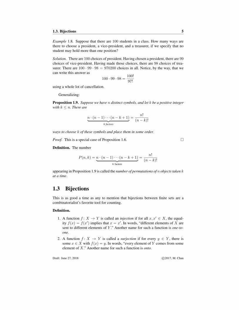
Example 1.8. Suppose that there are 100 students in a class. How many ways arethere to choose a president, a vice-president, and a treasurer, if we specify that nostudent may hold more than one position?

Solution. There are 100 choices of president. Having chosen a president, there are 99choices of vice-president. Having made those choices, there are 98 choices of trea-surer. There are 100 · 99 · 98 = 970200 choices in all. Notice, by the way, that wecan write this answer as

100 · 99 · 98 =100!

97!

using a whole lot of cancellation.

Generalizing:

Proposition 1.9. Suppose we have n distinct symbols, and let k be a positive integerwith k ≤ n. There are

n · (n− 1) · · · (n− k + 1)︸︷︷︸k factors

=n!

(n− k)!

ways to choose k of these symbols and place them in some order.

Proof. This is a special case of Proposition 1.6.

Definition. The number

P (n, k) = n · (n− 1) · · · (n− k + 1)︸︷︷︸k factors

=n!

(n− k)!

appearing in Proposition 1.9 is called the number of permutations of n objects taken kat a time.

1.3 BijectionsThis is as good a time as any to mention that bijections between finite sets are acombinatorialist’s favorite tool for counting.

Definition.

1. A function f : X → Y is called an injection if for all x, x′ ∈ X , the equal-ity f(x) = f(x′) implies that x = x′. In words, “different elements of X aresent to different elements of Y .” Another name for such a function is one-to-one.

2. A function f : X → Y is called a surjection if for every y ∈ Y , there issome x ∈ X with f(x) = y. In words, “every element of Y comes from someelement of X .” Another name for such a function is onto.


6 1. Combinatorics

3. A function f : X → Y is called a bijection if it is both injective and surjective.

Drawing some illustrations of injective/surjective/bijective functions convincesus that bijections are one-to-one correspondences. Alternatively, suppose f is bothinjective and surjective. Surjectivity implies that every element y ∈ Y is the imageunder f of at least one x ∈ X; injectivity implies that every element y ∈ Y is theimage under f of at most one x ∈ X . Hence every element y ∈ Y is the imageunder f of exactly one x ∈ X , which is the definition of one-to-one correspondence.

In particular, we see that compositions of bijections are bijections. It is a goodexercise to convince yourself, and then prove, the following basic fact about bijec-tions:

Proposition 1.10. A function f : X → Y is a bijection if and only if f has a two-sided inverse, i.e., if and only if there is a function g : Y → X such that f ◦ g = 1Yand g ◦ f = 1X .

Now here is why bijections are so useful in combinatorics.

Theorem 1.11. (Bijective Correspondence Principle)

If X and Y are finite sets in bijective correspondencethen they have the same number of elements.

Bijective correspondence simply means that there exists a bijection from one set tothe other.

The claim made in Theorem 1.11 is obvious, right? Then we should be able toprove it.

Proof. Let |X| = n. What does that actually mean? Presumably, it means thatthere is a bijection between X and the set {1, . . . , n}. If so, then by composingthat bijection with a bijection between X and Y , we obtain a bijection between Yand {1, . . . , n}, so |Y | = n also.

One might view the set {1, . . . , n} as the refference n-element set sitting on a shelf atthe National Bureau of Standards. The point is that one way to count the elements in aset Y is simply to establish a bijection between Y and some set X whose cardinalityyou already know. This comes up constantly, and is extremely satisfying! In fact, onecould argue that this is the best and most explicit way to count things—the variousother methods that we discuss are but tricks that we use when we are unable toproduce an explicit bijection.

We will see many examples, starting straightaway in the next section.

1.4 SubsetsDefinition. For n ≥ 0 an integer, we denote the set {1, . . . , n} by [n]. Somewhatstrangely, this convention includes [0] = ∅.


1.4. Subsets 7

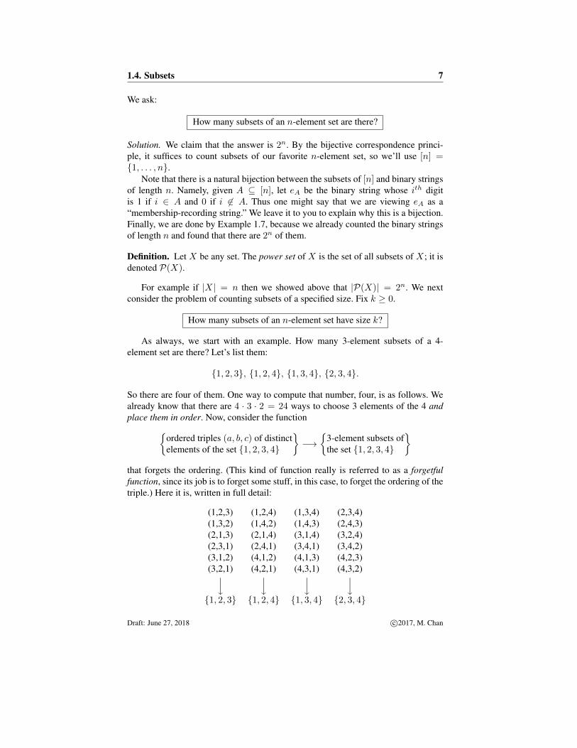
We ask:

How many subsets of an n-element set are there?

Solution. We claim that the answer is 2n. By the bijective correspondence princi-ple, it suffices to count subsets of our favorite n-element set, so we’ll use [n] ={1, . . . , n}.

Note that there is a natural bijection between the subsets of [n] and binary stringsof length n. Namely, given A ⊆ [n], let eA be the binary string whose ith digitis 1 if i ∈ A and 0 if i 6∈ A. Thus one might say that we are viewing eA as a“membership-recording string.” We leave it to you to explain why this is a bijection.Finally, we are done by Example 1.7, because we already counted the binary stringsof length n and found that there are 2n of them.

Definition. Let X be any set. The power set of X is the set of all subsets of X; it isdenoted P(X).

For example if |X| = n then we showed above that |P(X)| = 2n. We nextconsider the problem of counting subsets of a specified size. Fix k ≥ 0.

How many subsets of an n-element set have size k?

As always, we start with an example. How many 3-element subsets of a 4-element set are there? Let’s list them:

{1, 2, 3}, {1, 2, 4}, {1, 3, 4}, {2, 3, 4}.

So there are four of them. One way to compute that number, four, is as follows. Wealready know that there are 4 · 3 · 2 = 24 ways to choose 3 elements of the 4 andplace them in order. Now, consider the function{

ordered triples (a, b, c) of distinctelements of the set {1, 2, 3, 4}

}−→

{3-element subsets ofthe set {1, 2, 3, 4}

}that forgets the ordering. (This kind of function really is referred to as a forgetfulfunction, since its job is to forget some stuff, in this case, to forget the ordering of thetriple.) Here it is, written in full detail:

(1,2,3) (1,2,4) (1,3,4) (2,3,4)(1,3,2) (1,4,2) (1,4,3) (2,4,3)(2,1,3) (2,1,4) (3,1,4) (3,2,4)(2,3,1) (2,4,1) (3,4,1) (3,4,2)(3,1,2) (4,1,2) (4,1,3) (4,2,3)(3,2,1) (4,2,1) (4,3,1) (4,3,2)y y y y{1, 2, 3} {1, 2, 4} {1, 3, 4} {2, 3, 4}


8 1. Combinatorics

In general, each set downstairs has 6 = 3 · 2 · 1 elements sitting above it, where 6represents the number of ways to order the three given symbols. So we compute theanswer 4 as the solution to the problem ? · 6 = 24. More generally:

Definition. Let k, n ≥ 0 be integers with k ≤ n. We write(nk

)to denote the number

of k-element subsets of an n-element set. Such expressions are called binomial co-efficients, for reasons that will be clear soon. We note that this quantity is also calledthe number of combinations of n things taken k at a time and is sometimes denotedby C(n, k), but these days the notation

(nk

)is considered more stylish.

Proposition 1.12. We have(n

k

)=P (n, k)

k!=

n!

k!(n− k)!, (1.1)

where we recall that P (n, k) denotes the number of ways to choose k elements froman n-element set and order them.


Corollary 1.13. For each n ≥ 0, we have the following identity:

2n =

(n

0

)+

(n

1

)+ · · ·+

(n

n− 1

)+

(n

n

).

Proof. Both sides count the number of subsets of [n].

There is so much to say about the binomial coefficients! Let’s start by arrangingthem visually on the page in a big triangle, where the nth row goes from

(n0

)to(nn

).(

00

)(10

) (11

)(20

) (21

) (22

)(30

) (31

) (32

) (33

)This arrangement is commonly known as Pascal’s triangle, although it was inde-

pendently discovered and described by many mathematicians (and poets!) centuriesbefore Pascal’s book about it was published in 1665. A portion of Pascal’s triangle isillustrated in Figure 1.2.

Looking at Figure 1.2, we make some observations. Note that these are justguesses for the moment:

Conjecture 1.14. Pascal’s triangle has the following properties:(a) Each number, besides all the 1s, is the sum of the two numbers directly above.(b) The triangle is left-right symmetric.(c) Every number down the middle is even.(d) Every row is unimodal, meaning it first increases and then decreases.(e) If n is prime, then each

(nk

), other than

(n0

)and

(nn

), is a multiple of n.


1.4. Subsets 9

11 1

1 2 11 3 3 1

1 4 6 4 11 5 10 10 5 1

1 6 15 20 15 6 11 7 21 35 35 21 7 1

1 8 28 56 70 56 28 8 11 9 36 84 126 126 84 36 9 1

Figure 1.2: The first ten rows of Pascal’s triangle.

Proof. We prove the first statement of Conjecture 1.14 and leave the other parts ashomework; see Exercise 1.16. Conjecture 1.14(a) claim amounts to proving that theidentity (

n

k

)=

(n− 1

k

)+

(n− 1

k − 1

)is true for all integers n ≥ 1 and for all integers k satisfying 1 ≤ k ≤ n.

We could hash this out using the expression (1.1), but we’ll leave that for you,and we’ll take a more combinatorial, less computational, approach. We are goingto give a “bijective proof.” We consider the set X of k-element subsets of [n]. Forexample, if n = 4 and k = 2, then

X ={{1, 2}, {1, 3}, {1, 4}, {2, 3}, {2, 4}, {3, 4}

}.

We partition the set X into two subsets X1 and X2, where:• X1 consists of the sets that do not contain n;• X2 consists of the sets that do contain n.

So in our example with n = 4 and k = 2, we have

X1 ={{1, 2}, {1, 3}, {2, 3}

}and X2 =

{{1, 4}, {2, 4}, {3, 4}

}.

We note that X1 is in bijection with the set of k-element subsets of [n− 1], since,the sets in X1 are exactly the subsets of [n− 1]. And X2 is in bijection with theset of (k − 1)-element subsets of [n− 1], since each set in X2 is formed by taking ak − 1-element subset of [n− 1] and throwing in the element n. Alternatively, we candefine a bijection X2 → [n − 1] by taking a set in X2 and removing the element n.All in all, we find that(

n

k

)= |X| = |X1|+ |X2| =

(n− 1

k

)+

(n− 1

k − 1

),

which is exactly what we wanted to show.

Sometimes binomial coefficients are used to count things in unexpected ways:


10 1. Combinatorics

Example 1.15. You have n numbered boxes. How many ways are there to put kindistinguishable balls into them? Note tha “indistinguishable” means that we careonly about how many balls go in each box; the balls themselves are identical.

Solution. Convince yourself that you may count instead sequences consisting of ksymbols that look like • and n− 1 symbols that look like |. The circles represent theballs and the vertical bars represent box-separators. Here is an example of a sequenceof symbols and how it translates into balls in boxes:

• • | | • • • | • • corresponds to

Box 1

• •

Box 2 Box 3

• • •

Box 4

• •

The number of such sequences of circles and bars is(n− 1 + k

k

), since we can

view the problem as that of selecting k of the n − 1 + k symbols to be circles, andthen the other n− 1 symbols must be bars.

The method that we have used to solve this problem is sometimes referred to asthe “stars and bars” method (although we have used circles instead of stars), but atleast one mathematician from the Midwest has suggested that it should be called the“cows and fences” method.

Example 1.16. Same question as in Example 1.15, but now we require that every boxcontains at least one ball.

Solution. If n > k, then the answer is clearly 0, so we assume that n ≤ k. Then weneed to start by using k of the balls to put one in each box. This leave k−n balls to bedistributed in any way we please, so we are in the exactly situation of Example 1.15,except we only have k − n balls to put into the n boxes. So the answer is(

n− 1 + k − nk − n

)=

(k − 1

k − n

)=

(k − 1

n− 1

),

where for the second equailty comes we use the symmetry of Pascal’s triangle.

Finally we come to the binomial theorem, which will also tells us the origin ofthe name binomial coefficient. This theorem explains the pattern of the coefficientswhen we take powers of x+ y:

(x+ y)0 = 1

(x+ y)1 = 1x+ 1y

(x+ y)2 = 1x2 + 2xy + 1y2

(x+ y)3 = 1x3 + 3x2y + 3xy2 + 1y3

(x+ y)4 = 1x4 + 4x3y + 6x2y2 + 4xy3 + 1y4

...


1.5. The Principle of Inclusion-Exclusion 11

Theorem 1.17. (Binomial theorem) Let n ≥ 0 be an integer. We have the polynomialidentity

(x+ y)n =

n∑k=0

(n

k

)xkyn−k. (1.2)

Proof. One way to conceptualize a proof is to completely expand (x + y)n usingthe distributive law but without using commutativity just yet. For example, we mayexpand

(x+ y)(x+ y)(x+ y) = xxx+ xxy + xyx+ xyy + yxx+ yxy + yyx+ yyy.

In such an expansion, there are 2n terms (why?). Now collecting them together usingthe commutative law, we see that the term xkyn−k appears a total of

(nk

)times: this

is the number of binary sequences of length n made of k symbols x and n − ksymbols y.

Example 1.18. If we evaluate the formula (1.2) at x = y = 1, we get a new proof ofCorollary 1.13.

Example 1.19. Evaluating the formula (1.2) at x = 1 and y = −1 gives

0 = (1− 1)n =

n∑k=0

(n

k

)(−1)k =

∑k=0k even

(n

k

)−∑k=0k odd

(n

k

).

This shows that the number of subsets of [n] of even size equals the number of subsetsof [n] of odd size. Can you give a bijective proof of this fact?

There is a whole theory of multinomial coefficients as well, i.e., the coefficientsof

(x1 + · · ·+ xd)n

for some fixed d > 2. See if you can compute the multinomial coefficients andgeneralize the ideas in this section. If you are stuck, look them up!

1.5 The Principle of Inclusion-ExclusionHow many students are there who are on the chess team or the volleyball team?Let X1 be the set of students on the chess team, and let X2 be the set of students onthe volleyball team. Is the answer to our question simply |X1|+ |X2|?

No, not necessarily. If there are students who are on both teams, then we willhave overcounted. In order to correct for the overcounting, we need to subtract |X1∩X2|, which is the number of students on both teams. This is called the Principle ofInclusion/Exclusion, sometimes abbreviated as PIE.

Theorem 1.20. (Principle of Inclusion/Exclusion for two sets) IfX1 andX2 are finitesets, then

|X1 ∪X2| = |X1|+ |X2| − |X1 ∩X2|.


12 1. Combinatorics

Proof. Well, you probably already believe it, if you’re like 99% of people. The ideais that each element of X1 ∪ X2 is counted the same number of times on both leftand right. It is an exercise for you to make that statement entirely precise.

Similarly, if we have three sets that may have elements in common, then

|X1 ∪X2 ∪X3| = |X1|+ |X2|+ |X3| − |X1 ∩X2| − |X1 ∩X3| − |X2 ∩X3|+ |X1 ∩X2 ∩X3|,

and in general:

Theorem 1.21. (Principle of Inclusion/Exclusion, general case) Let n ≥ 1, andlet X1, . . . , Xn be finite sets. Then

|X1 ∪ · · · ∪Xn| =∑∅6=I⊆[n]

(−1)|I|−1∣∣∣∣⋂i∈I

Xi

∣∣∣∣. (1.3)

Proof. As in our proof sketch of Theorem 1.20, we verify that every element x ∈X1 ∪ · · · ∪Xn ends up contributing exactly one to the expression on the right handside of (1.3). Let

Jx = {i ∈ [n] : x ∈ Xi}.

For example, if x is in X1 and X3 and no other sets, then Jx = {1, 3}. On the righthand side of (1.3), we consider the terms in the sum that have a non-zero from x.These are exactly the terms where I is a subset so that x is in Xi for every i ∈ I , i.e.,these are exactly the terms where I is contained in Jx. And these terms are countedwith sign +1 if |I| is odd and with sign −1 if |I| is even.

Thus each x ∈ X1 ∪ · · · ∪Xn contributes exactly∣∣{I ⊆ Jx : |I| is odd}∣∣− ∣∣{I ⊆ Jx : |I| is even and I 6= ∅}

∣∣ (1.4)

to the right hand side of (1.3), and we need to show that (1.4) is equal to 1. But weknow from Example 1.19 that∣∣{I ⊆ Jx : |I| is odd}

∣∣ = ∣∣{I ⊆ Jx : |I| is even}∣∣,

and that gives the desired result, since in 1.4 we haven’t included the empty setamongthe sets with an even number of elements.

Example 1.22. (The problem of derangements). There are n people sitting on a com-pletely full airplane. The airline decides to wreak maximum havoc by reassigningseats in such a way that no person remains in the same seat. How many ways arethere to do this? Such a reassignment is called a derangement.

For example, for three people, there are six possible ways to rearrange them, butwe find that only two of those six permutations are derangements:

123 (all fixed), 132 (1 is fixed), 321 (2 is fixed), 213 (3 is fixed),312 (derangement), 231 (derangement).


1.5. The Principle of Inclusion-Exclusion 13

Solution. Let us temporarily assign numbers 1, . . . , n to the passengers. With norestrictions, there would be n! ways to reassign their seats. But that’s an overcount.For each i = 1, . . . , n, the ith passenger remains in their original seat for (n − 1)!of the possible n! permutations, so we need to subtract those off. But now we haveundercounted, because we’ve subtracted too many times if more than one passengeris in their original seat.

The Principle of Inclusion/Exclusion allows us to organize our successive over-counting and under-counting. For each i = 1, . . . , n, let

Xi = {seat reassignments in which the ith person stays in their seat}.

Note that ∪Xi is the set of all seat reassignments in which someone stays in theirseat, so the number that we seek is

# of derangements of [n] = n!− |X1 ∪ · · · ∪Xn|.

We are going to compute |X1 ∪ · · · ∪ Xn| using PIE. We note that if J ⊆ [n] is asubset of size j, then ∣∣∣∣⋂

i∈JXi

∣∣∣∣is the number of seat reassignments in which the people numbered by J stay in theirseat. There are (n − j)! ways for this to happen. Moreover, there are

(nj

)subsets

of [n] of size j. Applying PIE wile grouping together the subsets of [n] by size, givesthat

|X1 ∪ · · · ∪Xn| =n∑

j=1

(−1)j−1(n

j

)(n− j)!. (1.5)

So the number we want is n! minus the expression in (1.5), which we rewrite as

n!−n∑

j=1

(−1)j−1(n

j

)(n− j)! =

n∑j=0

(−1)j(n

j

)(n− j)! = n!

n∑j=0

(−1)j 1j!.

So we have proved the beautiful formula

# of derangements of [n] = n!

n∑j=0

(−1)j

j!.

If you have taken some calculus, you may recognize that the series∑∞

j=0(−1)j/j!converges to e−1 ≈ 0.368. So if n is large and you randomly choose a permuta-tion of [n], then there is roughly a 36.8% chance that your permutation will be aderangement.

Example 1.23. (Counting surjective functions). Let n and k be positive integers. Howmany surjective functions [n]→ [k] are there?


14 1. Combinatorics

Solution. This example is similar to Example 1.22. First, the multiplication rule saysthat there are kn functions [n] → [k]. Now for each i ∈ {1, . . . , k}, let Xi denotethe set of functions f : [n]→ [k] such that i is not in the image of f . In other words,there is no x ∈ [n] such that f(x) = i. The answer we seek, then, is

kn − |X1 ∪ · · · ∪Xk|.

Now let’s use PIE. We note that if J ⊆ [k] has size j, then∣∣∣∣⋂i∈J

Xi

∣∣∣∣ = (k − j)n.

So PIE says

# of surjective maps [n]→ [k] = kn − |X1 ∪ · · · ∪Xk|

= kn −∑

∅6=J⊆[k]

(−1)|J|−1∣∣⋂i∈J

Xi

∣∣= kn −

k∑j=1

∑J⊆([k]

j )

(−1)j−1(k − j)n

= kn −k∑

j=1

(−1)j−1(k

j

)(k − j)n

=

k∑j=0

(−1)j(k

j

)(k − j)n.

That’s the answer. An amusing side note is that if k > n, then since there are nosurjective maps [n] → [k], this last sum must equal 0. But this fact is is not at allclear if one just looks at the sum.

By the way, there is a closely related quantity that people sometimes refer to asthe Stirling numbers (of the second kind). (If you’re interested, you can look up theStirling numbers of the first kind.)

Definition. Let n and k be positive integers. We define the Stirling numbers of thesecond kind to be the quantities

S(n, k) =1

k!

k∑j=0

(−1)j(k

j

)(k − j)n,

So Example 1.23 says that the number of surjective functions [n]→ [k] is k!·S(n, k).The Stirling number S(n, k) also count somethng interesting, which in particular,implies that they are integers.

Proposition 1.24. The number of ways to divide a pile of n labeled objects intoexactly k piles is the Stirling number S(n, k).


1.6. The Erdos-Ko-Rado Theorem 15

Proof. If the k piles were labeled, this would be exactly the number of surjectivefuntions [n] → [k], where the image of each object tells us in which pile it sits, andthe surjectivity is required to ensure that we end up with exactly k piles. However,the piles are not supposed to be labeled, so we need to divide by the k! ways that wecan rearrange them. Hence the answer is

# of surjective maps [n]→ [k]

k!= S(n, k),

where we have used the formula for the number of surjective functions that we de-rived in Example 1.23.

1.6 The Erdos-Ko-Rado TheoremIn this section we describe a gem of extremal combinatorics. Extremal combinatoricsis a very beautiful part of combinatorics. It concerns understanding combinatorialstructures that are extremal, i.e., that are maximal or minimal with respect to somegiven property.

Fix positive integers r and n with r ≤ n. Your task is to find the largest possi-ble collection of r-element subsets of {1, . . . , n} subject to the following condition:every pair of subsets that you choose must have at least one element in common.

Definition. Let F be a collection of r-element subsets of [n]. We say that F is anintersecting family if for every S, T ∈ F , we have

S ∩ T 6= ∅.

We ask:

How large can an intersecting family of r-element subsets of [n] be?

For example, how large can an intersecting family of 2-element subsets of [4] be?Relabeling, we can always start with the subset {1, 2}. Our next subset must sharean element with {1, 2}, so after relabeling, they share 1 and the new element is 3,i.e., our second subset is {1, 3}. In order to form a third subset, we could take {1, 4},and then every pair of subsets shares 1, or we could take {2, 3}, in which case weagain get an intersecting family. And that’s as far as we can go. So the answer to ourquestion when n = 4 and r = 2 is that an intersecting family of 2-element subsetsof [4] contains at most 3 subsets, and that this can be achieved in two distinct ways(up to relabeling the elements),

F1 ={{1, 2}, {1, 3}, {1, 4}

}and F2 =

{{1, 2}, {1, 3}, {2, 3}

}(1.6)

We can generalize the construction of F1 to build an intersecting family,

F ={S ⊂ [n] : |S| = r and 1 ∈ S

}. (1.7)


16 1. Combinatorics

It is clear that F is an intersectng family, since every S ∈ F shares the commonelement 1. Furthermore,

|F| =(n− 1

r − 1

),

since each S ∈ F has the form {1}∪I for some (r−1)-element subset of {2, . . . , n},and there are

(n−1r−1)

choices for I .The following theorem says that the family F in (1.7) is the biggest that an inter-

secting family can be. This theorem was originally proved by Erdos, Ko, and Rado,but we give here is a later proof due to Katona in 1971.

Theorem 1.25. (Erdos-Ko-Rado theorem) Let n ≥ 2r be positive integers. Any in-tersecting family of r-elements subsets of [n] has size at most(

n− 1

r − 1

).

Proof. We define a cyclic ordering on [n], loosely, as an ordering of 1, 2, . . . , naround a clockwise oriented circle.2 For example, there are 6 cyclic orderingsof {1, 2, 3, 4}, as illustrated in Figure 1.3. In general there are (n − 1)! cyclic or-derings of [n].

1

2

3

4 C1

1

2

4

3 C2

1

3

2

4 C3

1

3

4

2 C4

1

4

2

3 C5

1

4

3

2 C6

Figure 1.3: The 6 cyclic orderings of {1, 2, 3, 4}

Next we say that a subset of [n] is an interval of a cyclic order if its elementsappear consecutively in the cyclic order. For example, in Figure 1.3 the set {3, 4} isan interval of C1, C2, C4, and C6, while {1, 2, 3} is an interval of all six of the Ci.We note that if n ≥ 24, then a given cycle C has exactly n intervals of length r,which are formed by starting at each element of C and taking the set consisting of rconsecutive elements. Thus the cycle C1 in Figure 1.3 has 4 intervals of length 2,namely {1, 2}, {2, 3}, {3, 4}, and {1, 4}.

2More precisely, a cyclic ordering is an equivalence class of cyclic permutations of {1, . . . , n}, underthe equivalence relation generated by a cyclic shift.


Exercises 17

Let F an intersecting family of r-element subsets of [n]. We are going to countthe elements of the following set in two different ways:

X ={(C, S) : C is a cyclic order and S is an interval of C with S ∈ F

}.

First, we count the elements of X by first choosing a set S ∈ F , which can bedone in |F| ways, then creating a cycle by putting the elements of S in some order,which can be done in r! ways, and then putting the elements of [n] that are not in Sin some order, which can be done in (n− r)! ways. So in total, we find that

|X| = |F| · r! · (n− r)!. (1.8)

Now let’s count the elements of X by first choosing the cycle C, which as wesaw earlier can be done in (n− 1)! ways, and then estimate how many S ∈ F can beintervals of the given C. We saw above that C contains n distinct intervals, but sincewe are restricting to intervals that are in the intersecting family F , we claim that atmost r members of F may appear as intervals of C.

To see why, suppose that I is an interval of C that is in F . We can shift I eitherclockwise or counterclockwise to get other intervals of C, but if we shift I too far,we’ll get an interval that has no elements in common with I , so it can’t be in F .More precisely, there are r−1 clockwise shifts of I that have an element in commonwith I , and similarly there are r−1 counterclockwise shifts of I that have an elementin common with I . But a clockwise shift I ′ and a counterclockwise shift I ′′ willhave no elements in common if the total shift for I ′ plus I ′′ is r or greater. Hencethe intersecting family F contains at most r elements that can appear as an intervalof C. In symbols, we have shown that

|X| ≤ (n− 1)! · r. (1.9)

Combining the two expressions (1.8) and (1.9) for |X|, we get

|F| · r! · (n− r)! ≤ (n− 1)! · r,

so

|F| ≤ (n− 1)! · rr! · (n− r)!

=(n− 1)!

(r − 1)!(n− r)!=

(n− 1

r − 1

),

which is exactly what we wanted to show.

Exercises

Section 1.1. The Pigeonhole Principle

1.1. Prove Theorem 1.2, the general version of the Pigeonhole Principle. Hint. Try to imitatethe proof of Theorem 1.1.

1.2. Prove the multiplication rule stated in Proposition 1.6. Hint. Give a proof by inductionon n, imitating the proof of Proposition 1.5.


18 Exercises

1.3. Suppose there are four rows of seats in a classroom, each row containing six seats. Howmany students are necessary to guarantee that no matter how they seat themselves, some rowwill be full?

Note that if you think the answer is N , then you need to argue both that N students forcea row to be full, but fewer than N students may seat themselves such that no row is full.

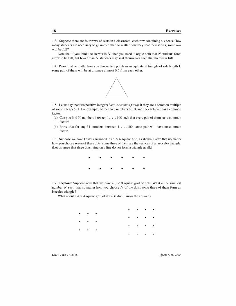
1.4. Prove that no matter how you choose five points in an equilateral triangle of side length 1,some pair of them will be at distance at most 0.5 from each other.

1.5. Let us say that two positive integers have a common factor if they are a common multipleof some integer> 1. For example, of the three numbers 6, 10, and 15, each pair has a commonfactor.

(a) Can you find 50 numbers between 1, . . . , 100 such that every pair of them has a commonfactor?

(b) Prove that for any 51 numbers between 1, . . . , 100, some pair will have no commonfactor.

1.6. Suppose we have 12 dots arranged in a 2× 6 square grid, as shown. Prove that no matterhow you choose seven of these dots, some three of them are the vertices of an isoceles triangle.(Let us agree that three dots lying on a line do not form a triangle at all.)

1.7. Explore: Suppose now that we have a 3 × 3 square grid of dots. What is the smallestnumber N such that no matter how you choose N of the dots, some three of them form anisoceles triangle?

What about a 4× 4 square grid of dots? (I don’t know the answer.)


Exercises 19

Section 1.2. Putting Things In Order

1.8. There are 100 students in a class, and we wish to choose a president, vice-president, andtreasurer. The only problem is that each student has a nemesis in the class, i.e., the class iscomprised of 50 pairs of nemeses, who can’t stand each other.

How many ways are there to choose a president, vice-president, and treasurer, so that notwo nemeses are chosen?

1.9. This exercise asks you to count numbers having certain properties.(a) How many 4-digit numbers are there that are not a multiple of 10?(b) How many 4-digit numbers are there whose digits sum to an even number?

Section 1.3. Bijections

1.10. Prove Proposition 1.10, which says that a function f : X → Y is a bijection if andonly if f has a two-sided inverse, i.e., if and only if there is a function g : Y → X suchthat f ◦ g = 1Y and g ◦ f = 1X .

1.11. How many bijections [n]→ [n] are there?

1.12. Let n > 1 be an integer.(a) How many ways are there to put the numbers 1, . . . , n in order such that 2 occurs imme-

diately after 1?(b) How many ways are there to put the numbers 1, . . . , n in order such that 2 occurs after 1

(but not necessarily immediately after it)?

1.13. Let a1, . . . , an be any positive numbers. Consider all the possible ways of writing a +or− sign before each ai. Prove that at most 2n−1 of these expressions produce a positive sum.For example, if we take 1, 3, and 4, then

+1 + 3 + 4 + 1− 3 + 4 − 1 + 3 + 4

are the three expressions producing a positive sum.

1.14. Let n be a positive integer. Let an be the number of ways to write n as a sum of oddpositive integers. Let bn be the number of ways to write n as a sum of distinct positive integers.In each case, order does not matter. For example, if n = 7, then we have

1 + 1 + 1 + 1 + 1 + 1 + 1, 1 + 1 + 1 + 1 + 3, 1 + 3 + 3, 1 + 1 + 5, 7

and1 + 2 + 4, 3 + 4, 2 + 5, 1 + 6, 7

so an = bn = 5.(a) Write out the various decompositions for n = 5 and n = 6, and verify that a5 = b5 and

a6 = b6.(b) Prove that an = bn for all n.

Section 1.4. Subsets

1.15. Prove Proposition 1.12, which says that the number of k-element subsets of an n elementset is given by the formula (

n

k

)=P (n, k)

k!=

n!

k!(n− k)! .


20 Exercises

1.16. Prove the remaining parts (b), (c), and (d) of Conjecture 1.14, although you may firstneed to formulate more rigorous versions.

1.17. In Example 1.19 we used the binomial formula to prove that the number of subsetsof [n] of even size equals the number of subsets of [n] of odd size. Give a bijective proof ofthis fact.

1.18. Let n ≥ 0 be an integer. Let An ⊆ P([n]) be the set of subsets [n] that do not containany consecutive pairs of numbers. For example,

A3 = {∅, {1}, {2}, {3}, {1, 3}} .

(a) Compute A0, A1, A2, A3, A4, A5.(b) Make a conjecture about the sequence of sizes |An| for all n ≥ 1.(c) Prove your conjecture.

1.19. Let n ≥ 0 be an integer. How many nested pairs of subsets of [n] are there? In otherwords, compute the size of the set

{(A,B) ∈ P([n])× P([n]) : A ⊆ B}.

Section 1.5. The Principle of Inclusion-Exclusion

1.20. This is a strength-training exercise in counting. Give a brief justification for each answer.Consider functions f : [6]→ [3].(A1) How many functions f are there?(A2) How many of them are surjective?(A3) How many of them take the value 1 exactly four times? By this we mean that there are

exactly four numbers i ∈ {1, . . . , 6} such that f(i) = 1.

(A4) How many of them are nondecreasing? By nondecreasing, we mean that

f(1) ≤ f(2) ≤ f(3) ≤ f(4) ≤ f(5) ≤ f(6).

(B1) How many of them are surjective and take the value 1 exactly four times?(B2) How many of them are surjective and nondecreasing?(B3) How many of them take the value 1 exactly four times and are nondecreasing?(B4) How many of them are surjective and nondecreasing and take the value 1 exactly four

times?(C1) How many of them are surjective or take the value 1 exactly four times?(C2) How many of them are surjective or nondecreasing?(C3) How many of them take the value 1 exactly four times or are nondecreasing?(C4) How many of them are surjective or nondecreasing or take the value 1 exactly four

times?Hint. : You may wish to use the Venn diagram in Figure 1.4 to organize your counting.

1.21. Of the numbers 1, . . . , 225, how many of them are relatively prime to 225? (Two posi-tive integers are called relatively prime if their greatest common divisor is 1.)

1.22. Explore: In the setting of Example 1.22, suppose one of the n! possible seat reassign-ments is chosen uniformly at random. On average, how many people stay in their seat?


Exercises 21

surjective

nondecreasing

1 appears four times

Figure 1.4: Venn diagram of functions [6]→ [3] for Exercise 1.20.

Section 1.6. The Erdos-Ko-Rado theorem

1.23. Fix an integer n > 0. Suppose F ⊆ P([n]) is an intersecting family of subsets of [n].In other words, for all S, T ∈ F we have S ∩ T 6= ∅.

(a) Prove that |F| ≤ 2n−1.(b) Find an example of an intersecting family F as above that has size exactly 2n−1.

Note: the difference between this problem and the Erdos-Ko-Rado theorem is that we nolonger require that all sets in F have the same fixed size.

1.24. Explore: Let n = 2r. The Erdos-Ko-Rado theorem says that there are at most(n−1r−1

)intersecting families of r-elements subsets of [n].

(a) If n > 2r, prove that every intersecting family F of r-elements subsets of [n] hasthe property that there is a common element in every S ∈ F . (Hint. Use this strongerassumption n > 24 in the proof of the Erdos-Ko-Rado theorem.)

(b) We saw in (1.6) that (a) is not true for r = 2 and n = 4, since {1, 2}, {1, 3}, {2, 3} is afamily of 2 element subsets of [4] where the subsets do not share a common element. Upto relabeling the elements, find all intersecting families of 3 element subsets of [6]. Howmany are there? Do the same for 4 element subsets of [8].


22 Exercises

(c) Show that every n = 2r, there is a family of r-elements subsets of [n] that do not sharea common element. Generalize (b) by finding a formual for the number of such families,up to relabeling.

(d) Same question as (c), but for n < 2r.


Chapter 2

Graph Theory

The first order of business is to define our primary object of study.

Definition. A graph G is a finite set V , whose elements are the vertices of G,together with a set E of unordered pairs of vertices, which are called the edgesof G.1

An unordered pair of vertices is simply a subset of V of size 2. We sometimesdenote the vertex and edge sets of G by V (G) and E(G), respectively, to emphasizethat they are associated to the graph G.

To save time and space, we often write an edge {i, j} as just ij. Thus, Figure 2.1shows a drawing of a graph G with vertex set V = {1, 2, 3, 4} and edge set

E = {{1, 2}, {2, 3}, {2, 4}, {3, 4}},

or E = {12, 23, 24, 34} for short.

12 3

4

Figure 2.1: A drawing of a graph G.

You can draw a graph by drawing points to represent the vertices, and line seg-ments connecting the points to represent the edges. (Of course, a given graph may bedrawn in many different ways.) Thus in some sense, you have already studied graphtheory if you ever did “Connect-the-Dots” drawings as a child. But in saying that, wedon’t mean to trivialize the field of graph theory. Although graphs are easy to define,

1For those readers who are really keeping track of minutae, we stipulate that V ∩ E = ∅. In practice,it suffices to always take V = [n] for some integer n and then never again have to worry about this issue.


24 2. Graph Theory

there are plenty of deep theorems about them. We will see a few of these theoremsin this chapter.

In addition, graphs are quite useful as structures on which to build models ofmany real-world phenomena, in particular phenomena that have to do with pairwiseinteractions across a collection of agents. For example, many models of networks,such as social networks, computer networks, transportation networks, etc., are builtusing the data structure of graphs.

2.1 GraphsIn this section we take G = (V,E) to be a graph.

Definition. Let v, w ∈ V be vertices of G, and let e ∈ E be an edge of G.

1. The edge e is incident to the vertex v if e contains v, in which case we alsosay that v is an endpoint of e.

2. If vw is an edge of G, then v and w are adjacent vertices, or neighbors, ofthat edge.

3. The degree of the vertex v, denoted deg(v), is the number of edges incidentto v. The degree of v is also sometimes called the valence of v.

Example 2.1. Suppose that there are 41 people at a party, and suppose that each pairof people either know each other or don’t know each other. Then I claim that someoneat the party knows an even number of people. How could we possibly deduce sucha fact from so little information? The answer is provided by the following little gemfrom graph theory.

Proposition 2.2. Let G = (V,E) be a graph. If every vertex of a graph has odddegree, then G has an even number of vertices. In other words,

deg(v) odd for every v ∈ V =⇒ |V | is even.

Proof. Consider the set

H ={(v, e) ∈ V × E : e is incident to v

}.

A good way to visualize such a pair (v, e) is as a “half-edge” in the graph, i.e., anedge with exactly one of its endpoints, as in the following picture:

We know tha each edge has exactly exactly two endpoints, so we can count thenumber of elements of H by computing

|H| =∑e∈E

∣∣{v ∈ V : v is an endpoint of e}∣∣ = ∑

e∈E2 = 2|E|.

In particular, we see that |H| is even.


2.1. Graphs 25

Alternatively, we can count the elements of H by summing over vertices v andcounting how many edges are incident to v. This gives the formula

|H| =∑v∈V

∣∣{e ∈ E : e is incident to v}∣∣ = ∑

v∈Vdeg(v).

We are told that deg(v) is odd for every vertex v, number, whereas we know that |H|is even. So we have shown that

Even Number = (Odd Number) + (Odd Number) + · · ·+ (Odd Number)︸︷︷︸|V | terms in the sum

.

The only way for this to happen is to have |V | even.

Actually, we proved something stronger than the statement in Proposition 2.2,namely that in any graph, the number of odd-degree vertices is even, which is aconsequence of the formula

2|E| =∑v∈V

deg(v) (2.1)

that we proved. The proof of (2.1) is a good example of the technique of double-counting, that is, counting the same thing two different ways in order to deduce theequality of the two counts.

2.1.1 A Zoo of Graphs

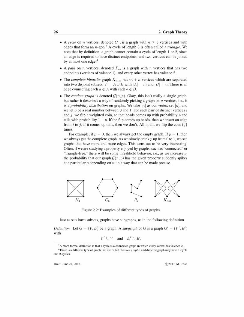
There are many different special kinds of graphs. Here are some nice examples tokeep in mind. See Figure 2.2.

• The complete graph on n vertices is a graph with n vertices such that thereis an edge joining every pair of vertices. Typically one uses [n] as the vertexset [n], and then the edge set is2

([n]

2

):= {S ⊆ [n] : |S| = 2}.

The complete graph on n vertices is denoted Kn.

Question 2.3. How many edges are there in Kn?

• The empty graph on n vertices is a graph with n vertices and no edges.

2Here we have employed a useful expansion of our combinatorial symbol notation. Thus for any set Tand integer k ≥ 0, we write

(Tk

)to denote the collection of k-element subsets of T . With this notation,

by definition we have∣∣∣(Tk)∣∣∣ =

(|T |k

).


26 2. Graph Theory

• A cycle on n vertices, denoted Cn, is a graph with n ≥ 3 vertices and withedges that form an n-gon.3 A cycle of length 3 is often called a triangle. Wenote that by definition, a graph cannot contain a cycle of length 1 or 2, sincean edge is required to have distinct endpoints, and two vertices can be joinedby at most one edge.4

• A path on n vertices, denoted Pn, is a graph with n vertices that has twoendpoints (vertices of valence 1), and every other vertex has valence 2.

• The complete bipartite graph Km,n has m + n vertices which are separatedinto two disjoint subsets, V = A ∪B with |A| = m and |B| = n. There is anedge connecting each a ∈ A with each b ∈ B.

• The random graph is denoted G(n, p). Okay, this isn’t really a single graph,but rather it describes a way of randomly picking a graph on n vertices, i.e., itis a probability distribution on graphs. We take [n] as our vertex set [n], andwe let p be a real number between 0 and 1. For each pair of distinct vertices iand j, we flip a weighted coin, so that heads comes up with probability p andtails with probability 1− p. If the flip comes up heads, then we insert an edgefrom i to j; if it comes up tails, then we don’t. All in all, we flip the coin

(n2

)times.

For example, if p = 0, then we always get the empty graph. If p = 1, thenwe always get the complete graph. As we slowly crank p up from 0 to 1, we seegraphs that have more and more edges. This turns out to be very interesting.Often, if we are studying a property enjoyed by graphs, such as “connected” or“triangle-free,” there will be some threshhold behavior, i.e., as we increase p,the probability that our graph G(n, p) has the given property suddenly spikesat a particular p depending on n, in a way that can be made precise.

K4 C6 P5 K3,3

Figure 2.2: Examples of different types of graphs

Just as sets have subsets, graphs have subgraphs, as in the following definition.

Definition. Let G = (V,E) be a graph. A subgraph of G is a graph G′ = (V ′, E′)with

V ′ ⊆ V and E′ ⊆ E.3A more formal definition is that a cycle is a connected graph in which every vertex has valence 2.4There is a different type of graph that are called directed graphs, and directed graph may have 1-cycle

and 2-cycles.


2.1. Graphs 27

12 3

4

Graph G

12

4

Subgraph G′ of G

Figure 2.3: The graph G from Figure 2.1 and a subgraph G′ of G

Note that the endpoints of an edge e ∈ E′ must be vertices in V ′, no “edges tonowhere” are allowed. This condition is enforced by the requirement that G′ is itselfa graph. Therefore, the elements of E′ are 2-element subsets of V ′. An example isshown in Figure 2.3.

We now introduce a concept that is both simple and deep: isomorphism. It isoften the case that we are interested in the structure of a graph, but we don’t careabout the exact names of the vertices. For example, at some level we would like totreat the two graphs in Figure 2.4 as the same, even though they are not literally thesame, since for instance, their vertex sets are different.

12 3

4

AB C

D

Figure 2.4: Two isomorphic graphs

So we define two graphs to be isomorphic if one is obtained from the other byrelabelling the vertices, as is described more precisely in the following definition.

Definition. Let G = (V,E) and G′ = (V ′, E′) be graphs. An isomorphism G→ G′

is a bijection f : V → V ′ with the property that for i, j ∈ V ,

ij ∈ E if and only if f(i)f(j) ∈ E′.

(We recall that ij is shorthand for {i, j}, and similarly f(i)f(j) is shorthand for{f(i), f(j)

}.)

If you are given two very small graphs, such as the ones in Figure 2.4, it is easyto tell whether they are isomorphic. But for graphs with many vertices and edges, thegeneral problem of determining whether two graphs are isomorphic is very difficult.This Graph Isomorphism Problem is one of the deep problems in computationalcomplexity.

Definition. Let G and G′ be graphs. We say that G contains G′ if G′ is isomorphicto a subgraph of G.


28 2. Graph Theory

12 3

4

12

3

4

5

6

7

Figure 2.5: Examples of Trees

We now have the terminology to define some interesting properties of graphshaving to do with whether they contain a fixed subgraph. An important one for ourpurposes is the property of not containing any cycles.

Definition. A graph G is acyclic if it does not contain any cycle Cn for any n ≥ 3.(We recall that C1 and C2 are not actually graphs.)

Now let us make a very simple observation: IfG is acyclic, then it remains acyclicafter removing any edges. Do you agree? This suggests that it could be interesting tostudy maximally acyclic graphs. By this we mean a graph G that is acyclic, but suchthat if we put in any single additional new edge connecting two of its vertices, thenthe augmented graph contains a cycle.

A graph that is maximal with respect to the property of being acyclic is called atree. They are of fundamental importance in graph theory. We study tress in the nextsection, although we define them there somewhat differently.

2.2 TreesFirst, we define what it means for a graph to be connected: it means that we can startat any vertex and take a walk in the graph to get to every other vertex.

Definition. A graph G is connected if it contains a path between any two vertices.

This is the kind of property that you would want if, say, you ran an airline. Youwould want your network of cities and direct flights to be connected, so that a cus-tomer could travel from any city to any other city on your flights.

A graph T is a tree if it is minimally connected.

In other words, a graph T is a tree if it is connected, but removing any edge wouldmake it disconnected. Thus it’s connected, but just barely, there’s no redundancy inthe connectivity.5 See Figure 2.5 for some examples of trees.

Let’s try to understand the structure of trees. First, we observe that trees areacyclic. After all, if there were a cycle, then removing an edge e lying in the cyclewould not disconnect the graph. (Do you see why?) In fact, we have the followingcharacterization of trees.

5And of course, the graph theory name for a graph that is a disjoint union of trees is a forest.


2.2. Trees 29

Proposition 2.4. A graph G is a tree if and only if G is connected and acyclic.

Proof. If G is a tree, then it is connected by definition, and furthermore we justestablished that it is acyclic as well.6

Suppose G is connected and acyclic. We need to show that G is minimally con-nected, i.e., we need to prove that given any edge ij of G, deleting ij disconnectsthe graph. We give a proof by contradiction, so we suppose G remains connected ifwe remove some particular edge ij. This means that G contains a path P from i to jother than the edge ij. But then P together with ij is a cycle, contradicting that G isacyclic.

There are many equivalent characterizations of trees, some of which you willencounter in the exercises.

Definition. A leaf of a tree is a vertex of degree 1.

We now establish that trees have leaves!

Proposition 2.5. Trees have leaves. More precisely, if T is a tree on at least twovertices, then T has at least two leaves.7

Proof. First, let’s give the idea. Suppose you are sitting around on the middle of anedge ij of T , and you want to find a leaf. What would you do? You would startwalking towards i and then keep walking, and walking, until you reach a dead end.That dead end is a leaf. If you go in the other direction toward j instead, you’d get asecond leaf. The point is that you cannot loop back to any previously visited vertex,because trees are acyclic.

Now we give the official proof.The assumption that T has at least 2 vertices and is connected means that T

contains at least one edge, so T contains some non-trivial paths. Let P be a maximalpath in T , i.e., the path P has the property that it is not contained in a longer pathof T .

Let ` and m be the endpoints of P . The ` is incident to an edge of P , as is m, soin particular deg(`) ≥ 1 and deg(m) ≥ 1.

We claim that the vertices ` and m have degree at most 1. To see why, supposethat deg(`) ≥ 2. We already know that there is a vertix x ∈ P that is adjacent to `.Suppose that there were some other y ∈ T that is adjacent to `. If y /∈ P , the wecan extend P to y. This creates a longer path, which contradicts our choice of P . Onthe other hand, if y ∈ P , then the edge `y together with the path in P from y to ` isa cycle, contradicting the assumption that T is acyclic. Hence deg(`) ≤ 1, and thesame argument gives deg(m) ≤ 1. Therefore ` and m are leaves of T .

Corollary 2.6. Every tree on n vertices has exactly n− 1 edges.

6Actually, we asked you to establish that it is acyclic; see Exercise 2.3.7Although we would be remiss if we didn’t mention that a tree with infinitely many vertices may

have 0 or 1 leaf!


30 2. Graph Theory

Proof. Here’s a sketch of a proof: If n = 1, there are no edges, so the statement isclear. For larger n, remove a leaf and its incident edge, and use induction.

How many trees are there on n vertices {1, . . . , n}?

It’s great counting practice to count trees on n vertices for n = 1, 2, 3, 4, 5, . . . .What do you get?

If you try to do this, you may start to suspect that in order to count labelledstructures, such as trees with labels 1, . . . , n assigned to their vertices, it is usefulto be able to count unlabelled structures and to understand how many symmetries(self-isomorphisms) they have. This is deep problem. It provides motivatation forunderstanding the idea of symmetries and symmetry groups, even if all one wants todo is to count stuff. The idea of symmetry features prominently in the Algebra unitof the course.

In any case, if you make a table for the first few values of n, you may be led toguess the following result.

Theorem 2.7. (Cayley’s Tree Counting Theorem) Let n > 1 be an integer. Thereare nn−2 trees on the vertex set {1, . . . , n}.

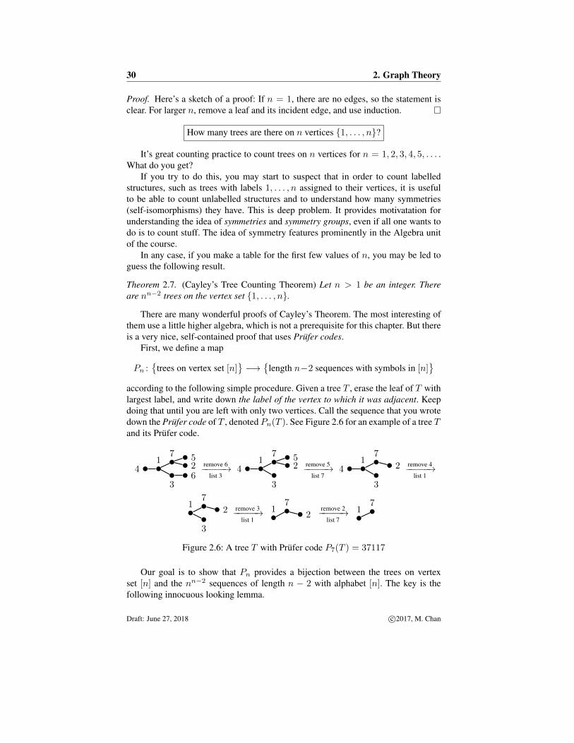
There are many wonderful proofs of Cayley’s Theorem. The most interesting ofthem use a little higher algebra, which is not a prerequisite for this chapter. But thereis a very nice, self-contained proof that uses Prufer codes.

First, we define a map

Pn :{

trees on vertex set [n]}−→

{length n−2 sequences with symbols in [n]

}according to the following simple procedure. Given a tree T , erase the leaf of T withlargest label, and write down the label of the vertex to which it was adjacent. Keepdoing that until you are left with only two vertices. Call the sequence that you wrotedown the Prufer code of T , denoted Pn(T ). See Figure 2.6 for an example of a tree Tand its Prufer code.

41

7

3

526

remove 6−−−−−→list 3

41

7

3

52 remove 5−−−−−→

list 74

17

3

2 remove 4−−−−−→list 1

17

3

2 remove 3−−−−−→list 1

17

2remove 2−−−−−→

list 71

7

Figure 2.6: A tree T with Prufer code P7(T ) = 37117

Our goal is to show that Pn provides a bijection between the trees on vertexset [n] and the nn−2 sequences of length n − 2 with alphabet [n]. The key is thefollowing innocuous looking lemma.


2.3. Graph Coloring 31

Lemma 2.8. Let T be a tree on vertex set [n]. Then the leaves of T are precisely thevertices not appearing in the Prufer code of T .

Proof. If a number i appears in Pn(T ), that means that at some point there was anedge incident to i whose other endpoint was a leaf, and the leaf and edge were rippedoff. So i is not a leaf.

If i is not a leaf, then it has at least two incident edges. At least one of theseedges must have been ripped off at some point. Consider the exact moment when thefirst of these edges was ripped off; it couldn’t have been that i was the leaf, since ihad degree at least 2. Therefore a leaf was ripped off of the other end of an edgecontaining i, so i appears in Pn(T ).

Incidentally, Lemma 2.8 shows that if you are given a Prufer code Pn(T ), butyou don’t know T , you can at least determine one small thing that’s true about T .Namely, if v is the largest vertex not in Pn(T ), then the first thing that was done wasto rip the leaf v off of the vertex whose label is recorded first in Pn(T ). Amazingly,this fact is all that we need to give an inductive proof of Cayley’s Theorem.

Proof of Cayley’s Theorem (Theorem 2.7). Given a sequence S = s1 · · · sn−2 whereeach si ∈ {1, . . . , n}, we want to show that S is the Prufer code of exactly one tree T .In other words, we need to show that Pn is a bijection. That claim is definitely truefor n = 2, which furnishes the base case of our induction.

Now suppose that n > 2. We will assume that Pn−1 is a bijection, and we’lldeduce that Pn is also a bijection. (This is how induction works.) So, suppose that Tis a tree with Pn(T ) = S. We’d like to show that exactly one such T exists.

Let ` be the largest element in [n] not appearing in the Prufer code S =s1s2 · · · sn−2. We know the following two things:

• Lemma 2.8 says that T has a leaf ` attached to the vertex s1.

• After deleting the leaf ` and its edge, the remaining tree T ′ on vertices [n]\{l}has Prufer code s2 · · · sn−2.

But now we are done! By induction, the tree T ′ with Prufer code s2 · · · sn−2exists and is unique, and the two conditions determine a unique T from the given T ′

and `, i.e., we must take T ′ and attach the leaf ` to the vertex s1. So T also exists andis unique.

This proof may annoy you a little, because we have not directly described aprocedure for taking a Prufer code and recovering a tree. This is a nice problem foryou to try.

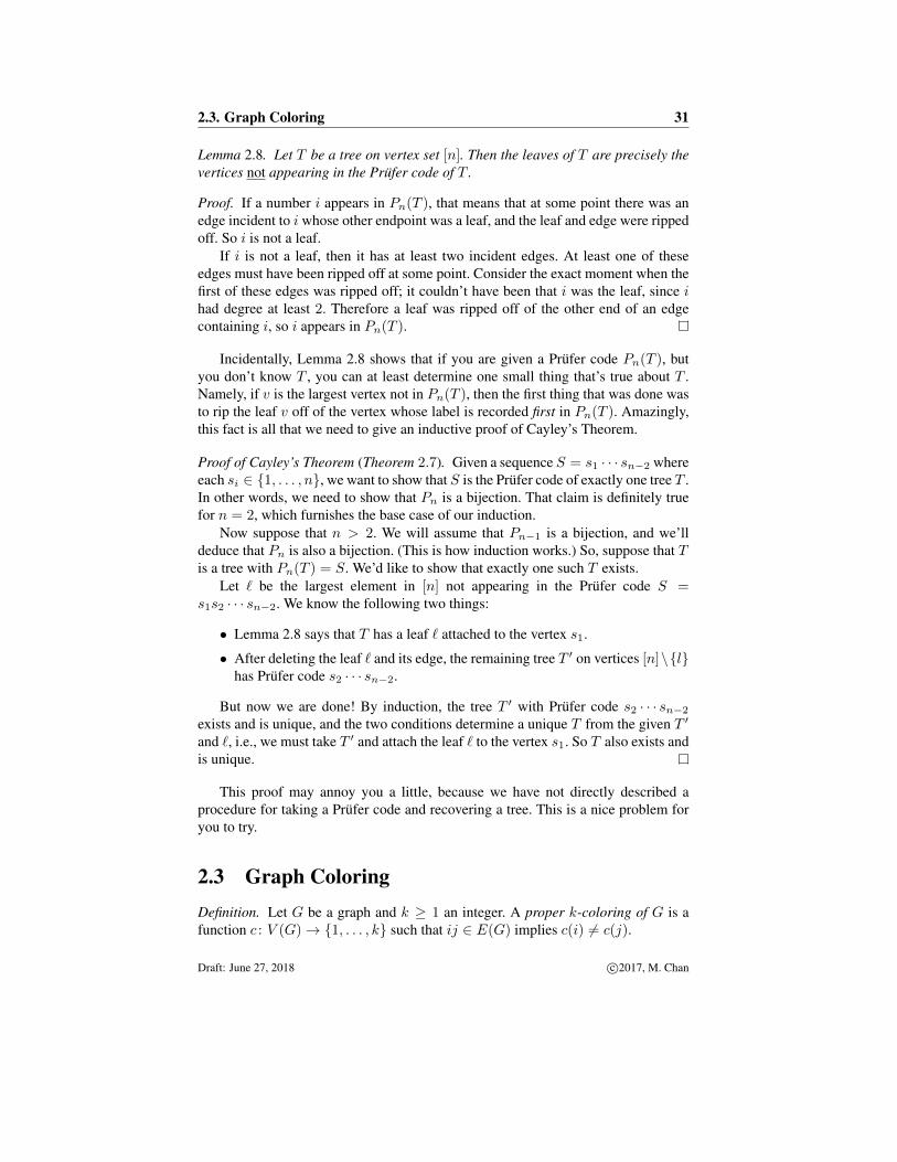
2.3 Graph ColoringDefinition. Let G be a graph and k ≥ 1 an integer. A proper k-coloring of G is afunction c : V (G)→ {1, . . . , k} such that ij ∈ E(G) implies c(i) 6= c(j).


32 2. Graph Theory

We view {1, . . . , k} as being a set of “colors,” and c describes a way to assign acolor to each vertex. With that in mind, the map c : V (G) → S is a proper coloringif adjacent vertices get different colors.

One of the most well-studied numbers that associated to a graph G is its chro-matic number.

Definition. The chromatic number of G, denoted χ(G),8 is the smallest positive in-teger k such that G has a proper k-coloring.

Example 2.9. Let n ≥ 3 be an integer. What is the chromatic number of the cy-cle Cn? We claim that the answer is as follows:

χ(Cn) =

{2 if n is even,3 if n is odd.

We give an informal argument, just to get a feel for chromatic numbers. Figure 2.7shows how to 3-color C5 and how to 2-coloring of C4. It is clear how to generalizethese examples to 2-color Ceven and to 3-color Codd. It remains to show that we can’tdo better.

First, since n ≥ 3, we clearly need at least 2 colors, so χ(Cn) ≥ 2. This handlesthe case that n is even. Suppose that n is odd and that we have a 2-coloring of Cn.Start at a vertex that has color 1 and trace the vertices clockwise around the cycle.They must be colored alternately 12121 · · · . But since n is odd, when we get backto the original vertex, we’ll be stuck with adjacent vertices that are both colored 1.Hence we need a third color.

*1

* 2

* 1*2

*3

*1 * 2

* 1*2

Figure 2.7: A 3-coloring of C5 and a 2-coloring of C4

Example 2.10. At the other extreme, the complete graph Kn on n vertices has chro-matic number χ(Kn) = n. This is clear, since every pair of vertices are connectedby an edge, so every vertex needs its own color. On the other hand, the completebipartite graph Km,n is 2-colorable, that is, χ(Km,n) = 2. This, too, is clear, sincetaking the vertices to be V = A ∪ B as in the definition of Km,n, we use one colorfor the vertices in A and a second color for the vertices in B. See Exercise 2.11 for aconverse statement.

8This is the Greek letter χ, pronounced “ki”. It is the first letter of the Greek word χρωµατικoς forchromatic.



It is useful to unpack the definition of chromatic number slowly. We observe thatfor any graph G:

(a) χ(G) ≤ k holds precisely when G has a proper k-coloring.

(b) χ(G) > ` holds precisely when G does not have any proper `-coloring.

Do you agree? These will be useful statements when proving things about chromaticnumbers. To illustrate, we prove the following simple statement.

Proposition 2.11. If H is a subgraph of G then χ(H) ≤ χ(G).

Proof. Write k = χ(G) for short, and let c : V (G) → [k] be a proper k-coloringof G. But then c : V (H) → [k] is a proper k-coloring of H , since if two verticesare adjacent in H , then they are also adjacent in G, and hence are assigned differentcolors by c. Therefore χ(H) ≤ k = χ(G), which is what we wanted to show.

A Personal Anecdote. In 2005, Professor Chan was a student at the Kneisel HallChamber Music Festival in Blue Hill, Maine. Each of the 55 or so students in theprogram is assigned to two chamber groups, which are small ensembles composedof 3-6 students. Every summer the director has to slot the 27 or so chamber groupsinto a daily rehearsal schedule. Of course, she can’t have the same student assignedto two groups rehearsing at the same time.

Question. Do you see what this scheduling problem have to do with graph coloring?

When Professor Chan arrived that summer, a friend “volunteered” her to write acomputer program to solve the Kneisel Hall scheduling problem, so that the directorwould no longer have to spend hours and hours overnight each summer doing thescheduling by hand. Almost every summer since then, she still uses graph-coloringalgorithms to do the scheduling of all the rehearsals and coachings at Kneisel Hall—as a sort of mathematician’s “in-kind donation.”

2.3.1 Planar Graphs and the Four and Five Color TheoremsLet G be a graph.

Definition. We say that G is planar if it can be drawn in the plane, i.e., on a sheet ofpaper, without edge crossings.

We will be somewhat informal about what exactly a drawing is, but what youpicture in your mind is likely to be correct. Namely, a drawing consists of a placementof the vertices of G at distinct points of your sheet of paper, and edges drawn in areasonable non-intersecting way, e.g. using a finite sequence of line segments orsmooth curves.9

It is important to note that planarity is a property of an abstract graph: it assertsthe existence of a drawing in the plane without edge-crossings. It does not assert that

9For those of you who think we are being too uptight about this, we want to inform, or remind, youthat space-filling curves exist. You can look up space-filling curves.


34 2. Graph Theory

any particular drawing has no edge-crossings. For example, the graph K4 is a planargraph, as illustrated in right-hand picture in Figure 2.8, even though if you were todraw K4 the first way that pops into your head, it might well be as the left-handpicture in Figure 2.8 that has an edge-crossing.

K4 with a edge crossing K4 drawn as a planar graph

Figure 2.8: Drawing K4 as a planar graph

Suppose that you want to draw a map of the world, with all the countries coloredin various shades. As is usual with maps, you impose the condition that two borderingcountries receive different colors.

What does this have to do with graphs? Draw a vertex inside each country. Then,if two countries share a border, draw an edge between their vertices crossing theborder. The resulting graph is called the dual graph, and the map-coloring questionbecomes a question of properly coloring the dual graph.

Mapmakers over the ages have long known, heuristically at least, that four colorsare always enough.

Theorem 2.12. (The Four Color Theorem) Every planar graph is 4-colorable.

This theorem is a cornerstone of combinatorial mathematics. It eluded prooffor several centuries. The first proof was given by Appel and Haken in 1976, butthe proof relied on computers so heavily that it was regarded as not being human-checkable, which upset some people. A simpler proof, but still relying on computers,was obtained decades later by Robertson, Sanders, Seymour, and Thomas, and in2005, Werner and Gonthier gave a formalized computer-readable proof.

The four color theorem sits at an interesting crossroads in mathematical culture,exposing differences in our perspectives on what proof really is. Does a proof needto be entirely human-understandable to really be a proof? After all, humans makemistakes all the time in verifying proofs. But what is a proof other than an argumentused by one human being to convince another of a mathematical truth? What do youthink?

Unsurprisingly, we will not prove the four color theorem in this text. But we willprove the five color theorem.

Theorem 2.13. (The Five Color Theorem) Every planar graph is 5-colorable.

This result was proven by Heawood in 1890 while exposing an error of a pur-ported proof by Kempf of the four color theorem published in 1879. It is remarkable



that it then took more than a century to squeeze that fifth color out of the theoremstatement!

Before proving the five color theorem, we first state a result that we will usewithout proof. First of all, if G is a planar graph, equipped with a fixed drawing onyour sheet of paper, we define a face to be a region of the complement of G. Thisincludes the infinite “outer” face that surround the entire graph.

Intuitively, if you take scissors and cut your paper along all of the edges of G,then the faces are the pieces of paper that are left over. The formula that we needgives a beautiful relationship satisfies by the vertices, edges, and faces.

Proposition 2.14. (Euler’s Polyhedron Formula) Let G be a connected graph drawnin the plane, with v vertices, e edges, and f faces. Then

v − e+ f = 2.

Euler’s Formula is a deep theorem that you will likely discuss in the Geometryunit. By the way, a special case of this formula states that any polyhedron in R3 atall, e.g., a cube, a tetrahedron, a dodecahedron, etc., satisfies v − e + f = 2 for itsvertices, edges, and faces. Do you see why this statement about polyhedra followsfrom Proposition 2.14?

As we now prove, a consequence of Euler’s formula is that every planar graphhas a vertex of degree at most 5.

Lemma 2.15. Every planar graph has a vertex of degree at most 5.

Proof. We may as well prove that every connected planar graph G has a vertex ofdegree at most 5. Suppose to the contrary that G is a connected planar graph andthat every vertex of G has degree 6 or more. Consider a plane drawing of G with vvertices, e edges, and f faces.

We start by by double-counting the set of edge-face incidences, i.e. the set ofordered pairs

EF :={(b, c) : b is an edge bounding the face c

}.

We note that each edge bounds exactly 2 faces, and every face is bounded by at least 3edges (since the boundary of a face is a cycle in G). This allows us to double-countthe set EF :

|EF | =∑

b∈E(G)

∣∣{c ∈ F (G) : b is an edge of c}∣∣ = 2

∣∣E(G)∣∣ = 2e.

|EF | =∑

c∈F (G)

∣∣{b ∈ E(G) : b is an edge of c}∣∣ ≥ 3

∣∣F (G)∣∣ = 3f.

Hence3f ≤ |EF | = 2e, so f ≤ 2

3e.

Next we double-count the set VE of vertex-edge incidences, i.e. the set of orderedpairs


36 2. Graph Theory

VE :={(a, b) : a is a vertex incident to the edge b

}.

Using the fact that every edge has exactly 2 endpoints and the assumption that everyvertex is incident to at least 6 edges, we double-count/estimate:

|VE| =∑

a∈V (G)

∣∣{b ∈ E(G) : a is incident to b}∣∣ ≥ 6

∣∣V (G)∣∣ = 6v.

|VE| =∑

b∈E(G)

∣∣{a ∈ V (G) : a is incident to b}∣∣ = 2

∣∣E(G)∣∣ = 2e.

Thus6v ≤ |VE| = 2e, so v ≤ 1

3e.

Using the estimates f ≤ 23e and v ≤ 1

3e, we find that

v − e+ f ≤ 2

3e− e+ 1

3e = 0,

which contradicts Euler’s Formula (Lemma 2.14).

We are ready to prove the five color theorem. Our strategy will be to delete astrategically chosen vertex v of G, inductively color the rest of G, and then showthat things may be arranged so that there is still a color available for v.

Proof. (Proof of Theorem 2.13, the Five Color Theorem) We wish to show that everyplanar graph is 5-colorable. We induct on the number of vertices. It is obvious thata 1-vertex graph is 5-colorable; indeed, it is 1-colorable! Now suppose that n > 1and that we have already proved that every graph with n− 1 vertices is 5-colorable.Let G be a planar graph on n vertices. We need to show that G is 5-colorable.

It is enough to prove the statement for connected planar graphs, since once we dothat, then we can 5-color any planar graph by 5-coloring its connected componentsone at a time. So we may assume that G is connected.

Let v ∈ V (G) be a vertex of degree at most 5. The existence of such a vertexis asserted in Lemma 2.15. Let G′ denote the graph obtained from G by deleting vand the 5 edges incident to v. Then our inductive hypothesis says that we can find a5-coloring c : G′ → [5] of G′.

If v has degree less than 5, then we win by coloring v using a color not yetused on any of its neighbors. Note that such a color exists because there are 5 colorsavailable, but v has at most 4 neighbors. So we may assume that deg(v) = 5.

Let v1, . . . , v5 be the neighbors of v, ordered clockwise around v, as illustratedin Figure 2.9. If 2 or more of those 5 neighbors are the same color, then there is acolor left over that we can use for v. So we may assume that v1, . . . , v5 use up all 5colors, i.e., c(v1), . . . , c(v5) are distinct.

We make the following simple observation: if the proper coloring of G′ may betweaked in some way so that at most 4 colors are used on v1, . . . , v5, then as above,we win.


2.4. Ramsey Theory 37

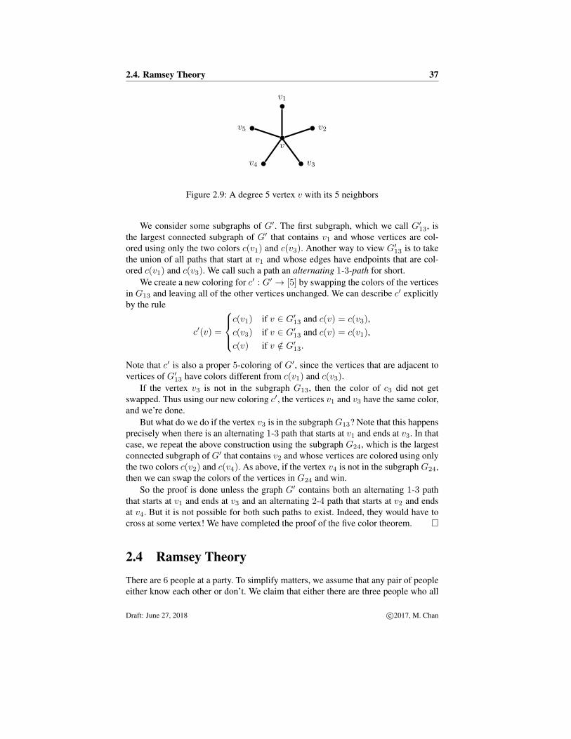
v1

v2

v3v4

v5

v

Figure 2.9: A degree 5 vertex v with its 5 neighbors

We consider some subgraphs of G′. The first subgraph, which we call G′13, isthe largest connected subgraph of G′ that contains v1 and whose vertices are col-ored using only the two colors c(v1) and c(v3). Another way to view G′13 is to takethe union of all paths that start at v1 and whose edges have endpoints that are col-ored c(v1) and c(v3). We call such a path an alternating 1-3-path for short.

We create a new coloring for c′ : G′ → [5] by swapping the colors of the verticesin G13 and leaving all of the other vertices unchanged. We can describe c′ explicitlyby the rule

c′(v) =

c(v1) if v ∈ G′13 and c(v) = c(v3),c(v3) if v ∈ G′13 and c(v) = c(v1),c(v) if v /∈ G′13.

Note that c′ is also a proper 5-coloring of G′, since the vertices that are adjacent tovertices of G′13 have colors different from c(v1) and c(v3).

If the vertex v3 is not in the subgraph G13, then the color of c3 did not getswapped. Thus using our new coloring c′, the vertices v1 and v3 have the same color,and we’re done.

But what do we do if the vertex v3 is in the subgraphG13? Note that this happensprecisely when there is an alternating 1-3 path that starts at v1 and ends at v3. In thatcase, we repeat the above construction using the subgraph G24, which is the largestconnected subgraph of G′ that contains v2 and whose vertices are colored using onlythe two colors c(v2) and c(v4). As above, if the vertex v4 is not in the subgraph G24,then we can swap the colors of the vertices in G24 and win.

So the proof is done unless the graph G′ contains both an alternating 1-3 paththat starts at v1 and ends at v3 and an alternating 2-4 path that starts at v2 and endsat v4. But it is not possible for both such paths to exist. Indeed, they would have tocross at some vertex! We have completed the proof of the five color theorem.

2.4 Ramsey Theory

There are 6 people at a party. To simplify matters, we assume that any pair of peopleeither know each other or don’t. We claim that either there are three people who all


38 2. Graph Theory

know each other, or there are three people who all don’t know each other. This is anexample of Ramsey theory, which is a beautiful topic that we explore in this section.

We can formulate this statement in terms of coloring the edges of K6, the com-plete graph on 6 vertices.

Definition. Let G be a graph G, and let k ≥ 1 be an. A k-edge-coloring of G is afunction

E(G)→ [k]

that assigns a color to each edge of G.

As usual, you may want to visualize an edge-coloring as an assignment of kactual colors to the edges of the graph. We can now formulate the previous claim asfollows:

Proposition 2.16. Every 2-edge-coloring of K6 contains a monochromatic triangle.

Remember that a triangle just means a C3 subgraph, which is the same as a K3

subgraph. Figure 2.10 shows some examples of 2-edge colorings of K6 with two orthree monochromatic triangles as indicated. Can you find a coloring of K6 that hasonly one monochromatic triangle?

Do you see why Proposition 2.16 is a rephrasing of the original claim? Let the 6people be the vertices ofK6, and color an edge blue if its endpoint people know eachother and red if they do not. Then a blue triangle gives three people who know eachother, and a red triangle give three people who don’t know each other.

AB

C

DE

F

ACD and BEF

AB

C

DE

F

ADE and ADF and BEF

AB

C

DE

F

ABC and DEF

Figure 2.10: Some 2-edge colored K6 graphs with indicated monochromatic trian-gles

Proof. For psychological ease, we label the vertices 1, . . . , 6, and call the colorsred and blue. There are five edges incident to vertex 1, and only two colors, so thePigeonhole Principle tells us that three of these edges are the same color, which wemay as well assume is red. So there are edges 1i, 1j, and 1k that are red.

If any of the three edges ij, ik, or jk are red, then we have found an edge thatcompletes a monochromatic red triangle. On the other hand, if ij, ik, or jk areall blue, then they form a monochromatic blue triangle. So in either case we geta monochromatic triangle, and we are done.


2.4. Ramsey Theory 39

We mention that Proposition 2.16 cannot be improved for monochromatic trian-gles in 2-edge-coloring, since it is possible to 2-edge-color the complete graph K5

such that there are no monochromatic triangles. See Exercise 2.15. Thus the num-ber 6 is some kind of threshhold, since it is the smallest number of vertices whichforces the existence of a red K3 or a blue K3.

Let’s think bigger. Is there any party that we could throw that’s big enough toguarantee that either there are 100 people who all know each other or there are 1000people who are all strangers to one another? Note that we definitely need to inviteat least 1000 people, since otherwise we could invite 999 pairwise-strangers. But it’salso clear that 1000 isn’t going to be enough. What do you think?

The question is whether there is always a threshhold, like the number 6 that wefound earlier, or whether instead it is possible to have bigger and bigger parties suchthat the people who know each other, and conversely the people who don’t, do notcome in large clumps.

Definition. Let k, ` ≥ 1 be integers. We define the (k, `)-Ramsey number, de-noted R(k, `), to be the smallest number n, if such a number exists, such that ev-ery 2-edge-coloring of Kn using colors red and blue contains either a red Kk, or ablue K`, or both.

So we have rephrased the question as: Do Ramsey numbers exist? For example,Proposition 2.16 says that R(3, 3) exists and satisfies R(3, 3) ≤ 6, and combinedwith Exercise 2.15 we see that R(3, 3) = 6.

Proposition 2.17. For all integers k, ` ≥ 1, the Ramsey number R(k, `) exists.

This is rather amazing. We model the proof on our proof that R(3, 3) ≤ 6.

Proof. We first note that for every k ≥ 1 and ` ≥ 1, we have

R(1, `) = R(k, 1) = 1.

This is clear, since a monochromatically edge-colored K1 is a vacuous condition,amounting to asking for the existence of at least one vertex.

Now, suppose we have established thatR(k′, `′) exists whenever k′ ≤ k and `′ ≤`, and suppose further that at least one of these inequalities is strict. We wish to showthat R(k, `) exists. (Thus, we are running an induction argument on N2

>0. Do youagree with the validity of this induction?) In fact, we shall show that R(k, `) existsand that

R(k, `) ≤ R(k − 1, `) +R(k, `− 1). (2.2)

In other words, we shall show that if n = R(k − 1, `) + R(k, ` − 1), then any2-edge-coloring of Kn has a red Kk or a blue K`.

Indeed, given a 2-edge-coloring of Kn, consider the

n− 1 = R(k − 1, `) +R(k, `− 1)− 1

edges incident to vertex 1. Among these, the Pigeonhole Principle implies that eitherthere are R(k − 1, `) red edges or there are R(k, ` − 1) blue edges. Let us suppose


40 2. Graph Theory

that there are R(k− 1, `) red edges incident to vertex 1; the other case can be arguedanalogously.

We consider the R(k − 1, `) vertices at the other ends of these red edges. By theinductive hypothesis, there is either a red Kk−1 or a blue K` among them. In thesecond case, we win. In the first case, we also win, since the red Kk−1 together withthe vertex 1 forms a red Kk.

Three colors. Why stop at two colors? Suppose that you are given three in-tegers k, `,m ≥ 1. Does there exist an n such that every 3-edge-coloring of KN

contains a red Kk, a blue K`, or a green Km?

Definition. Let k, `,m ≥ 1 be integers. We define the (k, `,m)-Ramsey number,denoted R(k, `,m), to be the smallest number n, if such a number exists, such thatevery 3-edge-coloring of Kn using colors red, blue, and green contains a red Kk, ablue K`, or a green Km.

Proposition 2.18. For all integers k, `,m ≥ 1, the Ramsey numberR(k, `,m) exists.

Proof. We claim that R(k, `,m) exists and satisfies

R(k, `,m) ≤ R(k,R(`,m)

).

The idea is to suppose that we are temporarily unable to distinguish between blueand green.

Let n = R(k,R(`,m)

)and suppose we have a 3-edge-coloring of Kn. Con-

sider it as 2-edge-coloring of Kn using colors “red” and “blue-green.” Then Propo-sition 2.17 says that either there is a red Kk or a blue-green KR(`,m). In the firstcase we win. In the second case, remembering again the difference between blue andgreen, we see that the original coloring has a KR(`,m)-subgraph which is 2-edge-colored blue and green. By definition of R(`,m), this subgraph contains either ablue K` or a green Km, and again we are done.

This same idea may be extended to arbitrarily many colors.

Proposition 2.19. Let n ≥ 1 be an integer. For integers m1, . . . ,mn ≥ 1, thereexists a number N with the following property: for every n-edge-coloring of thecomplete graph KN , there is some i ∈ {1, . . . , n} so that KN contains a completesubgraph Kmi

whose edges are all colored i.

Proof. Exercise, imitating the proof of Proposition 2.18.

Definition. We write R(m1, . . . ,mn) for the smallest such N such that Proposi-tion 2.19 is true. It is called the (m1, . . . ,mn)-Ramsey number.

What about lower bounds on Ramsey numbers? Let’s unpack this. The statement

R(k, `) > n

means that there exists a 2-edge-coloring of Kn with no red Kk and no blue K`.For example, in Exercise 2.15 you will show that R(3, 3) > 5 by producing anappropriate 2-edge-coloring of K5.


2.5. The Probabilistic Method 41

Question 2.20. What is the best lower bound for R(3, 4) that you can find?

Imagine trying to find a lower bound for R(100, 100). It seems that you wouldhave to painstakingly construct a 2-edge-coloring of a truly enormous graph and thendemonstrate in some way that the graph contains no monochromaticK100 subgraphs.That sounds hard!

It turns out that there is an amazing way to get around this difficulty. It hinges ona crucial idea that has been a theme of this text: it is possible to prove that somethingexists without actually constructing it. It’s better, of course, to give a constructiveproof, but sometimes that can be very hard. For example, we haveseen several argu-ments by contradiction that show that something exists without necessarily giving away to find it. Instead, we simply assume that it does not exist, and then derive anabsurdity.

In the next section we discuss a remarkable idea, called the probabilistic method,that can sometimes be used to prove that something exists without actually con-structing it. We will apply this method to prove some lower bounds on Ramsey num-bers R(k, `).

2.5 The Probabilistic MethodSuppose that we want to demonstrate that there is at least one dog living in Boston.The best thing to do would be to provide a constructive proof, i.e., actually produce aspecific dog who lives in Boston. But we can’t always achieve a constructive proof,even though we’d like to.

Suppose instead that we have a mechanism, such as an alien spaceship, for scoop-ing up a random creature who resides in Boston. And suppose further—and this isthe mysterious part—that we can somehow separately demonstrate that there is apositive probability that the Boston creature who we scoop up is a dog. Then wehave proved that there exists a dog living in Boston! Why? Well, if there were nodogs living in Boston, then the aforementioned probability would be zero.

The above example was chosen to sound maximally ludicrous, even though themethod itself, when applied correctly, is not. We are simply hoping to impress uponyou the remarkable fact that the probabilistic method works, and indeed is an impor-tant method to working combinatorialists today.

In this section we follow the discussion on page 1 of Alon and Spencer’s bookThe Probabilistic Method [1]. It leads to a lower bound for Ramsey numbersR(k, k),discovered by Erdos in 1947.

Proposition 2.21. Let k ≥ 3 be an integer. If n is a positive integer satisfying(n

k

)· 21−(

k2) < 1, (2.3)

then R(k, k) > n.

Before proving the proposition, let’s assume that it’s true and get a sense for howgood a bound it gives for Ramsey numbers.


42 2. Graph Theory

Corollary 2.22. We have R(k, k) > 2k/2.

Proof of Corollary 2.22, assuming Proposition 2.21. We want to show that n =b2k/2c satisfies inequality (2.3). We shall use the following useful bound on sizesof binomial coefficients:(

n

k

)=n · (n− 1) · (n− k + 1)

k!≤ nk

k!.

So, if n = b2k/2c, then(n

k

)· 21−(

k2) ≤ (2k/2)k

k!· 21−(

k2) =

1

k!· 2

k2

2 +1−(k2) =1

k!· 21+ k

2 < 1.

(We leave it for you to check that the final inequality is true, e.g., by induction.) Thisis the desired result, and we’re done.

Now onward to the proof of Proposition 2.21.

Proof of Proposition 2.21. Let n be a positive integer satisfying the inequality (2.3).We want to show that there is a 2-edge-coloring of Kn with no monochromatic Kk.There are finitely many 2-edge-colorings of Kn. We pick one at random and shalldemonstrate that the probability that our randomly chosen coloring contains nomonochromatic Kk is positive. That’s the probabilistic method.

There are a total of 2(n2) distinct 2-edge-colorings ofKn, sinceKn has

(n2

)edges.

Let’s start by focusing our attention on one particularKk subgraph—for instance, theone on vertices {1, . . . , k}—and asking in how many of the 2-edge colorings of Kn

is this particular Kk monochromatic. The answer is

2 · 2(n2)−(

k2),

since there are two ways to monochromatically 2-color Kk, multiplied by all thedifferent ways to 2-color the other

(n2

)−(k2

)edges. And of course, this number does

not depend on the particular Kk subgraph of Kn that we chose.In order to figure out exactly how many of the 2-edge-colorings of Kn have

at least one monochromatic Kk subgraph, we could do some counting via inclu-sion/exclusion. But let’s not do that. Instead, we make the simple observation thatsince the number of Kk subgraphs in Kn is

(nk

), the number of 2-edge colorings in

which some Kk is monochromatic is at most

(number of Kk

subgraphs of Kn

)·

number of ways to 2-edge colorKn so that a specified Kk

subgraph is monochromatic

=

(n

k

)· 2(

n2)−(

k2)+1.

We conclude that the probability that a randomly chosen 2-edge-coloring of Kn

has a monochromatically colored Kk is at most


2.5. The Probabilistic Method 43(n

k

)· 2(

n2)−(

k2)+1

2(n2)

,

which is equal to (n

k

)· 21−(

k2).

This last quantity is smaller than 1 by hypothesis. In other words, if n satisfies thestated inequality (2.3), then some 2-edge-coloring of Kn has no monochromatic Kk.So R(k, k) > n.

To this day, the lower bounds on Ramsey numbers proven by the probabilisticmethod are better than those that have been given in a constructive manner, but thisis a topic of current research. It is also interesting that the only values of R(k, k) thatwe know exactly are R(1, 1) = 1, R(2, 2) = 2, R(3, 3) = 6, and R(4, 4) = 18. Forhigher values of k there are upper and lower bounds, for example 43 ≤ R(5, 5) ≤ 48and 102 ≤ R(6, 6) ≤ 165.

In fact, something tantalizing can be gleaned from the bound that we derivedfor R(k, k). We showed that if n = b2k/2c , then the probability that a random2-edge-coloring of Kn has no monochromatic Kk is 1

k! · 21+k/2. Not only is that

number smaller than 1 when k ≥ 3, it is much, much smaller than 1 when k large.For example, when k = 10 it is roughly 0.0000176, and when k = 100, it is smallerthan 10−142.

This says that a great way to construct a 2-edge coloring of Kn with nomonochromatic Kk is to pick a coloring at random. You should then check that theone you picked is a good one, but it’s very likely to be good. (The reason that thisisn’t the same as a constructive lower bound on Ramsey numbers is that it only dealswith one k at a time, and not all k at once.)

With hindsight, it’s reasonable that we appealed to a probabilistic method to ob-tain a lower bound on Ramsey numbers, since a lower bound asserts the existenceof a structure that is rather disordered, i.e., there are no large clumps of red and nolarge clumps of blue. Roughly speaking, if you try to write down 2-edge-coloringsin some systematic way, you will tend to find these large monochromatic clumps. Insome vague philosophical sense, that’s due to the very fact that you are being sys-tematic. On the other hand, a random 2-edge-coloring of Kbk/2c is likely to be notvery clumpy and thus do the trick.

This is a demonstration, at least morally, of an aptly named principle that is foundall over mathematics and computer science, the so-called difficulty of finding hay ina haystack.10 In practice, it can indeed be hard to find hay in a haystack, despite thefact that 99.9% (or whatever) of the haystack is made of hay, since every time yousystematically reach into the haystack and pull something out, you may find that it isa needle!

10This is from a 2017 talk “Finding Hay in Haystacks: The Power and Limits of Randomness” by math-ematician/computer scientist Avi Wigderson that may be viewed at https://simons.berkeley.edu/events/theoretically-speaking-avi-wigderson.


44 Exercises

One final remark: you might complain that we haven’t really used probability,as opposed to just counting, in a meaningful way. Indeed, in our proof of Propo-sition 2.21, we counted the number of 2-edge-colorings of Kn not containing amonochromatic Kk and showed that this number is smaller than the total numberof 2-edge-colorings of Kn. Your complaint is a good one. In this particular instance,everything we did can be phrased simply in terms of counting and without mentionof probabilities. However, in many situations the perspective of probability and theprobabilistic method, and the techniques they bring to bear, are very useful, evenwhen applied in purely combinatorial situations. That is a story for another time,which you can read about in [1]. For further reading, see Bona’s excellent text-book [2] on combinatorics and Diestel’s graduate level textbook [3] on graph theory.

Exercises

Section 2.1. Graphs

2.1. Prove that in any graph, there are two vertices having equal degree. (Hint. Assume not,and think about the set of vertex degrees.)

2.2. Let G and G′ be the two 6-vertex graphs shown below. How many isomorphisms (seepage 28) from G to G′ are there? Explain your answer briefly.

1

2

3

4

5

6

G

A

B

C

D

E

F

G′

Section 2.2. Trees

2.3. Let G be a graph that contains a cycle. Prove that G is not minimally connected, i.e.,prove that it is possible to remove an edge from G and still be left with a connected graph.

2.4. Prove that a graph G is a tree if and only if it is maximally acyclic. In other words, G isa tree T if and only the following two facts are true:• T is acyclic.• Adding a new edge connecting two vertices of T creates a cycle.

2.5. Draw six nonisomorphic trees on vertex set {1, 2, 3, 4, 5, 6}, and compute each of theirPrufer codes.

2.6. Let n ≥ 2 be an integer. Of the nn−2 trees on vertex set [n], prove that exactly 2nn−3

of them contain the edge {1, 2}. Here are two hints suggesting possible ways to sole thisproblem.

(i) Double-count the elements of the set{(T, {i, j}) : T is a tree with vertices [n] and {i, j} is an edge of T

}.


Exercises 45

(ii) Alternatively, prove carefully that a tree contains the edge {1, 2} if and only if its Prufercode ends in 1 or 2.

2.7. Let n ≥ 2 be an integer. Of the nn−2 trees on vertex set [n], in how many of them isvertex n a leaf?

2.8. Let m > n ≥ 2 be integers. Of the nn−2 trees on vertex set [n], how many haveexactly m leaves?

2.9. Explore: Let n ≥ 3 be an integer. Among the nn−2 trees on vertex set [n], what is theaverage number of leaves?

Section 2.3. Graph coloring

2.10. Let G be a graph, and let D be the maximum degree of its vertices. Prove that

χ(G) ≤ D + 1.

2.11. Let G be a graph that is 2-colorable, i.e., χ(G) = 2. Prove that G is a subgraph of acomplete bipartite graph Km,n with m+ n = |V |.

2.12. Let G be a graph on n vertices. The complement of G, denoted G, is the graph obtainedfrom G by changing edges to non-edges and non-edges to edges. In other words, ij ∈ E(G)if and only if ij 6∈ E(G). Prove that

χ(G) · χ(G) ≥ n.

2.13. The four-color theorem asserts that every planar graph is 4-colorable. Is the conversetrue? That is, is every 4-colorable graph planar?

2.14. Explore: Lemma 2.15 says that every planar graph has a vertex of degree at most 5. Tryto find a planar graph such that every vertex has degree exactly 5. Hint. Use Euler’s formulawith a double count of edge-face incidences and vertex-edge incidences, as in the proof ofLemma 2.15, to find the minimum number of vertices, edges, and faces that might work.

Section 2.4. Ramsey theory

2.15. Find a 2-edge-coloring of the complete graphK5 such that there are no monochromatictriangles.

2.16. Let k, ` ≥ 1 be positive integers. Prove that

R(k, `) ≤

(k + `− 2

k − 1

).

2.17. Consider an N × N square grid of dots, with rows and columns labeled 1, . . . , N .For n ≤ N , let S, T ⊆ [N ] be subsets of size n. An n× n square subgrid is the set of the n2

dots in rows S and columns T . In particular, square subgrids don’t have to be contiguous.(a) Given n ≥ 1, is it true that there exists a number N such that every 2-coloring of the

dots in an N ×N square grid contains an n× n monochromatic square subgrid?(b) If n = 2, can you calculate the smallest N with the property of part (a)?


Appendix A

Appendix: Class Exercises

These are the problems that we may work on during class.

A.1 Randomized PlaylistsSuppose you have 15 songs stored on a computer. A music service creates a 15-songplaylist for you by choosing one song at random from your collection for each of the15 slots. (So, for example, it is possible that it plays the same song 15 times, althoughthat is exceedingly unlikely.)(a) How many possible playlists are there?(b) Of the playlists in part (a), what percentage of them repeat at least one song?

First take a wild guess; then figure it out.(c) Of the playlists in part (a), what percentage of them repeat at least one song

twice in a row? First take a wild guess; then figure it out.(d) Explore: Of the playlists in part (a), what percentage of them repeat at least one

song k times in a row, when k = 3? What about k = 4, . . . , 15?

Note: On the whole, people tend to significantly underestimate the likelihood thata song repeats, or even repeats twice in a row. For this reason, music services likeSpotify or iTunes initially fielded many complaints from users that their playlist al-gorithms were defective. In some cases, these companies decided to rewrite theiralgorithms to make their playlists feel more random, even though the new methodswere actually less random!


A.2. Catalan Bijections 47

A.2 Catalan Bijections(a) Let n be a positive integer. Construct bijections between the following foursets.1

(1) The set Xn of walks from (0, 0) to (2n, 0) and consisting of 2n steps, eachstep in direction (1, 1) or (1,−1), with the property that the walk never crossesbelow the x-axis. For example:

(2) The set Yn of sequences of n open parenthesis symbols ( and n close paren-thesis symbols ) that are correctly parenthesized, meaning that in any initialsubsequence, one never encounters more close parentheses ) than open paren-theses (. For example, here are two valid sequences and one that is not valid:

( ( ) ( ( ) ) )︸︷︷︸a valid sequence

( ( ) ( ) ( ) )︸︷︷︸a valid sequence

( ( ) ) ) ( ( )︸︷︷︸an invalid sequence

(3) The set Zn of bijective assignments of the numbers 1, . . . , 2n to a 2 × n gridof boxes such that the rows increase from left to right and the columns increasefrom top to bottom. For example:

1 3 42 5 6

(4) The set Wn of triangulations of a convex polygon on n+ 2 vertices. A triangu-lation of a convex polygon P is a collection of noncrossing diagonals in P thatdivide it into triangles. For example:

(b) Compute the size of X4 and X5.(c) Make a conjecture about the sequence of sizes of the sets X1, X2, X3, . . . and

prove your conjecture.

1This exercise is inspired by Exercise 6.19 in Richard Stanley’s classic text Enumerative Combina-torics, Volume II.[4] However, instead of having only 4 sets, Stanley lists 66 sets asks the reader to comeup with

(662

)bijections!


48 A. Appendix: Class Exercises

A.3 How Many Trees?1. How many trees are there on vertex set {1}?

2. How many trees are there on vertex set {1, 2}?

3. How many trees are there on vertex set {1, 2, 3}?

4. How many trees are there on vertex set {1, 2, 3, 4}?

5. How many trees are there on vertex set {1, 2, 3, 4, 5}?

6. How many trees are there on vertex set {1, 2, 3, 4, 5, 6}?

Hint. You probably won’t want to actually try to draw all of them when thereare 5 or 6 vertices!


References

[1] N. Alon and J. H. Spencer. The probabilistic method. Wiley Series in DiscreteMathematics and Optimization. John Wiley & Sons, Inc., Hoboken, NJ, fourthedition, 2016.

[2] M. Bona. A walk through combinatorics. World Scientific Publishing Co., Inc.,River Edge, NJ, 2002. An introduction to enumeration and graph theory, With aforeword by Richard Stanley.

[3] R. Diestel. Graph theory, volume 173 of Graduate Texts in Mathematics.Springer-Verlag, New York, 1997. Translated from the 1996 German original.

[4] R. P. Stanley. Enumerative combinatorics. Vol. 2, volume 62 of CambridgeStudies in Advanced Mathematics. Cambridge University Press, Cambridge,1999. With a foreword by Gian-Carlo Rota and appendix 1 by Sergey Fomin.

[5] R. P. Stanley. Enumerative combinatorics. Volume 1, volume 49 of CambridgeStudies in Advanced Mathematics. Cambridge University Press, Cambridge,second edition, 2012.


Documents

Introduction to Higher Mathematics: Combinatorics …jhs/MA0075/IHM2.pdfIntroduction to Higher Mathematics: Combinatorics and Graph Theory Melody Chan (modiﬁed by Joseph Silverman)