Embed Size (px)
Citation preview

Introduction to Data Mining

Motivating Facts
Trends leading to Data Flood• More data is generated:
– Bank, telecom, other business transactions ...– Scientific data: astronomy, biology, etc– Web, text, and e-commerce
Big Data Examples • Europe's Very Long Baseline Interferometry (VLBI) has
16 telescopes, each of which produces 1 Gigabit/second of astronomical data over a 25-day observation session – storage and analysis a big problem
• AT&T handles billions of calls per day– so much data, it cannot be all stored -- analysis has to be done
“on the fly”, on streaming data
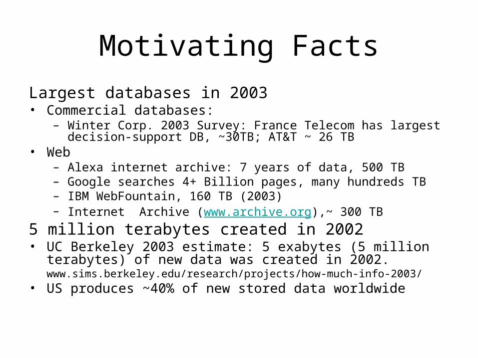
Largest databases in 2003• Commercial databases:
– Winter Corp. 2003 Survey: France Telecom has largest decision-support DB, ~30TB; AT&T ~ 26 TB
• Web– Alexa internet archive: 7 years of data, 500 TB– Google searches 4+ Billion pages, many hundreds TB – IBM WebFountain, 160 TB (2003)– Internet Archive (www.archive.org),~ 300 TB
5 million terabytes created in 2002• UC Berkeley 2003 estimate: 5 exabytes (5 million terabytes) of new
data was created in 2002.www.sims.berkeley.edu/research/projects/how-much-info-2003/
• US produces ~40% of new stored data worldwide
Motivating Facts

Historical Note: Many Names of Data Mining
• Data Fishing, Data Dredging: 1960-– used by Statistician (as bad name)
• Data Mining :1990 -- – used DB, business – in 2003 – bad image because of TIA
• Knowledge Discovery in Databases (1989-)– used by AI, Machine Learning Community
• also Data Archaeology, Information Harvesting, Information Discovery, Knowledge Extraction, ...
Currently: Data Mining and Knowledge Discovery are used interchangeably

Big Picture
• Lots of hype & misinformation about data mining out there
• Data mining is part of a much larger process – 10% of 10% of 10% of 10% – Accuracy not always the most important measure of data mining
• The data itself is critical • Algorithms aren’t as important as some people think • If you can’t understand the patterns discovered with data
mining, you are unlikely to act on them (or convince others to act)

Defining Data Mining
• The automated extraction of hidden predictive information from (large) databases
• Three key words: – Automated – Hidden – Predictive
• Implicit is a statistical methodology • Data mining lets you be proactive
– Prospective rather than Retrospective

Data Mining Is..
• Decision Trees
• Nearest Neighbor Classification
• Neural Networks
• Rule Induction
• K-means Clustering Algorithm
And more …

Data Mining is Not..
• Brute-force crunching of bulk data
• “Blind” application of algorithms
• Going to find relationships where none exist
• Presenting data in different ways
• A database intensive task• A difficult to understand
technology requiring an advanced degree in computer science

• DB’s user knows what is looking for.• DM’s user might/might not know what is looking for.• DB’s answer to query is 100% accurate, if data correct.• DM’s effort is to get the answer as accurate as possible.• DB’s data are retrieved as stored.• DM’s data need to be cleaned (some what) before
producing results.• DB’s results are subset of data.• DM’s results are the analysis of the data.• The meaningfulness of the results is not the concern of
Database as• it is the main issue in Data Mining.
Data Mining vs. Database

Convergence of Three Technologies
DM
Increasing Computing
Power
Statistical &Learning
Algorithms
ImprovedData
CollectionAnd Mgmt

1. Increased Computing Power– Moore’s law doubles computing power every 18 months – Powerful workstations became common – Cost effective servers provide parallel processing to the mass
market
2. Improved Data Collection– The more data the better (usually)

3. Improved Algorithms– Techniques have often been waiting for
computing technology to catch up– Statisticians already doing “manual data
mining” – Good machine learning is just the intelligent
application of statistical processes – A lot of data mining research focused on
tweaking existing techniques to get small percentage gains

Data Mining: On What Kind of Data?
• Relational databases
• Data warehouses• Transactional databases• Advanced DB and information repositories
– Object-oriented and object-relational databases– Spatial databases– Time-series data and temporal data– Text databases and multimedia databases– Heterogeneous and legacy databases– WWW

Data Mining Application areas
• Science– astronomy, bioinformatics, drug discovery, …
• Business– advertising, CRM (Customer Relationship
management), investments, manufacturing, sports/entertainment, telecom, e-Commerce, targeted marketing, health care, …
• Web: – search engines, bots, …
• Government– law enforcement, profiling tax cheaters, anti-terror(?)


Data Mining Tasks...
• Classification [Predictive]
• Clustering [Descriptive]
• Association Rule Discovery [Descriptive]
• Sequential Pattern Discovery [Descriptive]
• Regression [Predictive]
• Deviation Detection [Predictive]

Association Rules
• Given:– A database of customer transactions– Each transaction is a set of items
• Find all rules X => Y that correlate the presence of one set of items X with another set of items Y– Example: 98% of people who purchase diapers and
baby food also buy beer.– Any number of items in the consequent/antecedent of
a rule– Possible to specify constraints on rules (e.g., find only
rules involving expensive imported products)

Confidence and Support
• A rule must have some minimum user-specified confidence1 & 2 => 3 has 90% confidence if when a
customer bought 1 and 2, in 90% of cases, the customer also bought 3.
• A rule must have some minimum user-specified support1 & 2 => 3 should hold in some minimum
percentage of transactions to have business value

Example
• Example:
• For minimum support = 50%, minimum confidence = 50%, we have the following rules
1 => 3 with 50% support and 66% confidence
3 => 1 with 50% support and 100% confidence
Transaction Id Purchased Items 1 {1, 2, 3}2 {1, 4}3 {1, 3}4 {2, 5, 6}

Problem Decomposition - Example
TID Items1 {1, 2, 3}2 {1, 3}3 {1, 4}4 {2, 5, 6}
For minimum support = 50% = 2 transactionsand minimum confidence = 50%
Frequent Itemset Support{1} 75%{2} 50%{3} 50%{1, 3} 50%
For the rule 1 => 3:•Support = Support({1, 3}) = 50%•Confidence = Support({1,3})/Support({1}) = 66%

The Apriori Algorithm
• Fk : Set of frequent itemsets of size k • Ck : Set of candidate itemsets of size k F1 = {large items}for ( k=1; Fk != 0; k++) do { Ck+1 = New candidates generated from Fk
foreach transaction t in the database do Increment the count of all candidates in Ck+1 that are contained in t Fk+1 = Candidates in Ck+1 with minimum support }Answer = Uk Fk

Key Observation
• Every subset of a frequent itemset is also frequent
=> a candidate itemset in Ck+1 can be pruned if even one of its subsets is not contained in Fk

Apriori - Example
TID Items1 {1, 3, 4}2 {2, 3, 5}3 {1, 2, 3, 5}4 {2, 5}
Itemset Sup.{1} 2{2} 3{3} 3{4} 1{5} 3
Itemset Sup.{2} 3{3} 3{5} 3
Itemset{2, 3}{2, 5}{3, 5}
{2, 3} 2{2, 5} 3{3, 5} 2
Itemset Sup.{2, 5} 3
Database D C1 F1
C2 C2 F2
Scan D
Scan D

Partitioning
• Divide database into partitions D1,D2,…,Dp
• Apply Apriori to each partition
• Any large itemset must be large in at least one partition.

Partitioning Algorithm
1. Divide D into partitions D1,D2,…,Dp;
2. For I = 1 to p do
3. Li = Apriori(Di);
4. C = L1 … Lp;
5. Count C on D to generate L;

Partitioning Example
D1
D2
S=10%
L1 ={{Bread}, {Jelly}, {Bread}, {Jelly}, {PeanutButter}, {PeanutButter}, {Bread,Jelly}, {Bread,Jelly}, {Bread,PeanutButter}, {Bread,PeanutButter}, {Jelly, PeanutButter}, {Jelly, PeanutButter}, {Bread,Jelly,PeanutButter}}{Bread,Jelly,PeanutButter}}
L2 ={{Bread}, {Milk}, {Bread}, {Milk}, {PeanutButter}, {Bread,Milk}, {PeanutButter}, {Bread,Milk}, {Bread,PeanutButter}, {Milk, {Bread,PeanutButter}, {Milk, PeanutButter}, PeanutButter}, {Bread,Milk,PeanutButter}, {Bread,Milk,PeanutButter}, {Beer}, {Beer,Bread}, {Beer}, {Beer,Bread}, {Beer,Milk}}{Beer,Milk}}

Partitioning Adv/Disadv
• Advantages:– Adapts to available main memory– Easily parallelized– Maximum number of database scans is
two.
• Disadvantages:– May have many candidates during second
scan.
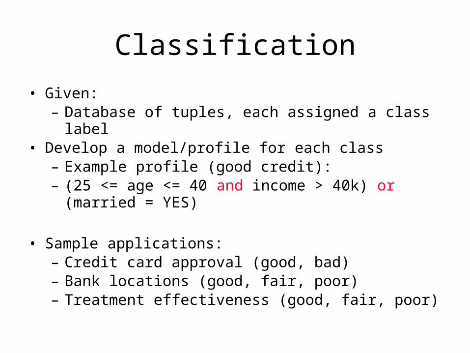
Classification
• Given:– Database of tuples, each assigned a class label
• Develop a model/profile for each class– Example profile (good credit):– (25 <= age <= 40 and income > 40k) or (married =
YES)
• Sample applications:– Credit card approval (good, bad)– Bank locations (good, fair, poor)– Treatment effectiveness (good, fair, poor)

Classification Example
Class C
(>50K)(<=50K)
c
Sample Decision Tree
ClassSalaryAgeJobTid
Industry
0
1
2
3
4
5
Univ.
Self
Self
Univ.
Industry
60K35
30
45
50
35
30
70K
60K
70K
40K
30K
B
A
B
C
C
C
Training Data Set
Sal
Age
(>40)(<=40)
Job
Class B Class A
Class C(Univ., Industry)
(Self)
Self6 60K35 A
Self7 70K30 A

Decision Tree
• Flow-chart like tree structure• Each node denotes a test on an attribute value• Each branch denotes outcome of the test• Tree leaves represent classes or class distribution• Decision tree can be easily converted into set of
classification rules

Example Decision Tree
Tid Refund MaritalStatus
TaxableIncome Cheat
1 Yes Single 125K No
2 No Married 100K No
3 No Single 70K No
4 Yes Married 120K No
5 No Divorced 95K Yes
6 No Married 60K No
7 Yes Divorced 220K No
8 No Single 85K Yes
9 No Married 75K No
10 No Single 90K Yes10
categoric
al
categoric
al
continuous
class
Refund
MarSt
TaxInc
YESNO
NO
NO
Yes No
Married Single, Divorced
< 80K > 80K
Splitting Attributes
The splitting attribute at a node is
determined based on the Gini index.

Decision Trees
• Pros– Fast execution time– Generated rules are easy to interpret by
humans– Scale well for large data sets– Can handle high dimensional data
• Cons– Cannot capture correlations among attributes– Consider only axis-parallel cuts

Regression
Mapping a data item to a real-value
E.g., linear regression
Risk score=0.01*(Balance)-0.3*(Age)+4*(HouseOwned)

Clustering– Identifies natural groups or clusters of instances.
Example: customer segmentation
– Unsupervised learning: Different from classification – clusters are not predefined but are formed based on the data
– Objects in each cluster are very similar to each other and are different from those in other clusters.

Customer Attrition: Case Study
• Situation: Attrition rate at for mobile phone customers is around 25-30% a year!
Task:
• Given customer information for the past N months, predict who is likely to attrite next month.
• Also, estimate customer value and what is the cost-effective offer to be made to this customer.

Customer Attrition Results
• Verizon Wireless built a customer data warehouse
• Identified potential attriters• Developed multiple, regional models• Targeted customers with high propensity to
accept the offer• Reduced attrition rate from over 2%/month to
under 1.5%/month (huge impact, with >30 M subscribers)
(Reported in 2003)

Assessing Credit Risk: Case Study
• Situation: Person applies for a loan
• Task: Should a bank approve the loan?
• Note: People who have the best credit don’t need the loans, and people with worst credit are not likely to repay. Bank’s best customers are in the middle

Credit Risk - Results
• Banks develop credit models using variety of machine learning methods.
• Mortgage and credit card proliferation are the results of being able to successfully predict if a person is likely to default on a loan
• Widely deployed in many countries

Successful e-commerce – Case Study
• A person buys a book (product) at Amazon.com.• Task: Recommend other books (products) this
person is likely to buy• Amazon does clustering based on books bought:
– customers who bought “Advances in Knowledge Discovery and Data Mining”, also bought “Data Mining: Practical Machine Learning Tools and Techniques with Java Implementations”
• Recommendation program is quite successful

Unsuccessful e-commerce case study (KDD-Cup 2000)
• Data: clickstream and purchase data from Gazelle.com, legwear and legcare e-tailer
• Q: Characterize visitors who spend more than $12 on an average order at the site
• Dataset of 3,465 purchases, 1,831 customers• Very interesting analysis by Cup participants
– thousands of hours - $X,000,000 (Millions) of consulting
• Total sales -- $Y,000• Obituary: Gazelle.com out of business, Aug 2000

Genomic Microarrays – Case Study
Given microarray data for a number of samples (patients), can we
• Accurately diagnose the disease?
• Predict outcome for given treatment?
• Recommend best treatment?

Example: ALL/AML data • 38 training cases, 34 test, ~ 7,000 genes
• 2 Classes: Acute Lymphoblastic Leukemia (ALL) vs Acute Myeloid Leukemia (AML)
• Use train data to build diagnostic model
ALL AML
Results on test data: 33/34 correct, 1 error may be
mislabeled
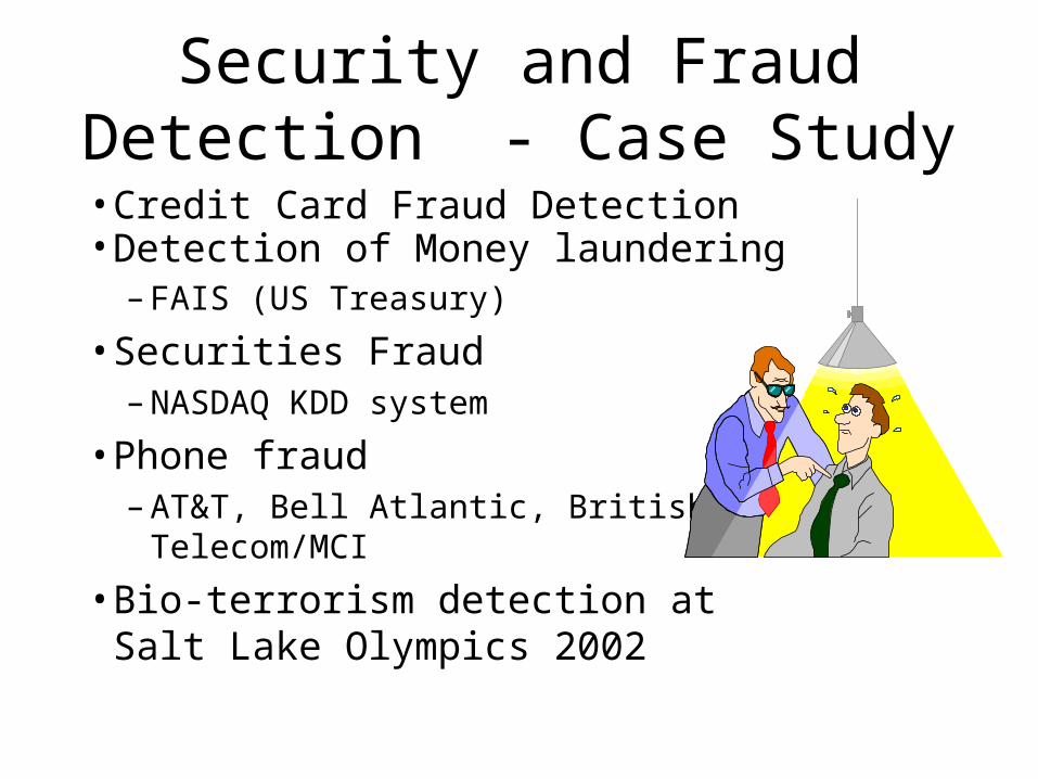
Security and Fraud Detection - Case Study
• Credit Card Fraud Detection• Detection of Money laundering
– FAIS (US Treasury)
• Securities Fraud– NASDAQ KDD system
• Phone fraud– AT&T, Bell Atlantic, British Telecom/MCI
• Bio-terrorism detection at Salt Lake Olympics 2002
Commercial Data Mining Software
• It has come a long way in the past seven or eight years• According to IDC, data mining market size of $540M in
2002, $1.5B in 2005 – Depends on what you call “data mining”
• Less of a focus towards applications as initially thought – Instead, tool vendors slowly expanding capabilities
• Standardization – XML
• CWM, PMML, GEML, Clinical Trial Data Model, … – Web services?
• Integration – Between applications – Between database & application

What is Currently Happening?
• Consolidation • Analytic companies rounding out existing product lines
– SPSS buys ISL, NetGenesis • Analytic companies expanding beyond their niche
– SAS buys Intrinsic • Enterprise software vendors buying analytic software
companies – Oracle buys Thinking Machines – NCR buys Ceres
• Niche players are having a difficult time • A lot of consulting • Limited amount of outsourcing
– Digimine

Top Data Mining Vendors Today
• SAS– 800 Pound Gorilla in the data analysis space
• SPSS • Insightful (formerly Mathsoft/S-Plus)
– Well respected statistical tools, now moving into mining • Oracle
– Integrated data mining into the database • Angoss
– One of the first data mining applications (as opposed to tools) • HNC
– Very specific analytic solutions • Unica
– Great mining technology, focusing less on analytics these days

Standards In Data Mining
– Predictive Model Markup Language (PMML) • The Data Mining Group (www.dmg.org) • XML based (DTD)
– Java Data Mining API spec request (JSR-000073) • Oracle, Sun, IBM, … • Support for data mining APIs on J2EE platforms • Build, manage, and score models programmatically
– OLE DB for Data Mining • Microsoft • Table based • Incorporates PMML
– It takes more than an XML standard to get two applications to work together and make users more productive

Privacy Issues
• DM applications derive demographics about• customers via• – Credit card use• – Store card• – Subscription• – Book, video, etc rental• – and via more sources…• As the DM results are deemed to be a good• estimate or prediction, one has to be sensitive to• the results not to violate privacy.

Final Comments
• Data Mining can be used in any organization that needs to find patterns or relationships in their data.
• DM analysts can have a reasonable level of assurance that their Data Mining efforts will render useful, repeatable, and valid results.

Resources and References
• Good overview book: – Data Mining Techniques
by Michael Berry and Gordon Linoff
• Web: – Knowledge Discovery Nuggets
• http://www.kdnuggets.com (ref-tutorials)
– http://www.thearling.com (ref-tutorials)
• DataMine Mailing List – [email protected] – send message “subscribe datamine-l”

Questions?