Embed Size (px)
Citation preview

Introduction to Computational Fluid Dynamics
Lecture 2 –Basic equations. Dimensionless parameters 1
Fluid Mechanics and Heat Transfer. Basic equations.
Continuity (Mass Conservation)
0vdiv
0
vdiv
t
Momentum Equation (Navier-Stokes equations)
Incompressible viscous fluid ( constant,constant )
vpgradFvvt
v
incompressible

Introduction to Computational Fluid Dynamics
Lecture 2 –Basic equations. Dimensionless parameters 2
Energy equation
Tgradkdivdt
dp
dt
dE
1
where E is the internal energy of a fluid particle (viscous compressible fluid)
- gas heating due to the compression
vdivpdt
dp
equationcontinuity
1
- mechanical work of the viscous forces transformation in heat

Introduction to Computational Fluid Dynamics
Lecture 2 –Basic equations. Dimensionless parameters 3
By taking into account that the enthalpy of a unit of mass is
pEi we
obtain
Tgradkdivdt
dp
dt
di
But for a perfect gas we have
dTcdi p
and energy equation becomes
Tgradkdivdt
dpTc
dt
dp
where
fv
t
f
Dt
Df
dt
df
is the substantial derivative.

Introduction to Computational Fluid Dynamics
Lecture 2 –Basic equations. Dimensionless parameters 4
Momentum Equation (for fluid saturated porous media)
By a porous medium we mean a material consisting of a solid matrix
with an interconnected void.
Porous media are present almost always in the surrounding medium, very
few materials excepting fluids being non-porous.
heat exchanger processor cooler porous rock

Introduction to Computational Fluid Dynamics
Lecture 2 –Basic equations. Dimensionless parameters 5
Darcy’s (law) equation (momentum equation)
gpgradK
v
where
v is the average velocity (filtration velocity, superficial velocity,
seepage velocity or Darcian velocity)
gkK is the permeability of the porous medium
Darcy’ law expresses a linear dependence between the pressure gradient
and the filtration velocity. It was reported that this linear law is not valid
for large values of the pressure gradient.

Introduction to Computational Fluid Dynamics
Lecture 2 –Basic equations. Dimensionless parameters 6
Darcy’s law extensions
Forchheimer’s extension
vvK
cv
Kp F
where Fc is a dimensionless parameter depending on the porous medium
Brinkman’s extension
vvK
p
~
where ~ is an effective viscosity
Brinkman-Forchheimer’s extension
vvvK
cv
Kp F
~

Introduction to Computational Fluid Dynamics
Lecture 2 –Basic equations. Dimensionless parameters 7
Energy equation for porous media
TkTvct
Tc efluidpmp
where
solidpfluidpmp ccc 1
solidfluide kkk 1

Introduction to Computational Fluid Dynamics
Lecture 2 –Basic equations. Dimensionless parameters 8
Bouyancy driven flow1
There exists a large class of fluid flows in which the motion is caused by
buoyancy in the fluid.
Buoyancy is the force experienced in a fluid due to a variation of density in
the presence of a gravitational field. According to the definition of an
incompressible fluid, variations in the density normally mean that the fluid is
compressible, rather than incompressible.
For many of the fluid flows of the type mentioned above, the density variation
is important only in the body-force term of the momentum equations. In all
other places in which the density appears in the governing equations, the
variation of density leads to an insignificant effect.
Buoyancy results in a force acting on the fluid, and the fluid would accelerate
continuously if it were not for the existence of the viscous forces.
The situation depicted above occurs in natural convection.
1 I.G. Currie, Fundamental Mechanics of Fluids, 3rd ed., Marcel Dekker, New York, 2003

Introduction to Computational Fluid Dynamics
Lecture 2 –Basic equations. Dimensionless parameters 9
Generally, density is a function of temperature and concentration
cT ,
Black Sea salinity, temperature
and density
(Ecological Modelling, 221,
2010, p. 2287-2301)

Introduction to Computational Fluid Dynamics
Lecture 2 –Basic equations. Dimensionless parameters 10
Boussinesq’s approximation
,
Momentum

Introduction to Computational Fluid Dynamics
Lecture 2 –Basic equations. Dimensionless parameters 11
Dimensionless equations
0
z
w
y
v
x
u
2
2
2
2
2
2
z
u
y
u
x
u
x
pF
z
uw
y
uv
x
uu
t
ux
2
2
2
2
2
2
z
v
y
v
x
v
y
pF
z
vw
y
vv
x
vu
t
vy
2
2
2
2
2
2
z
w
y
w
x
w
z
pF
z
ww
y
wv
x
wu
t
wz
0)q(2
2
2
2
2
2
z
T
y
T
x
Tk
z
Tw
y
Tv
x
Tu
t
Tcp
222222
222x
w
z
u
z
v
y
w
y
u
x
v
x
w
x
v
x
u

Introduction to Computational Fluid Dynamics
Lecture 2 –Basic equations. Dimensionless parameters 12
We introduce further the dimensionless variables
0t
t ,
L
xX ,
L
yY ,
L
zZ ,
0U
uU ,
0U
vV ,
0U
wW ,
g
FF
' ,
0p
pP ,
T
TT
0
into the governing equations
U
t
U
tUU
t
u
0
00 ,
X
U
L
U
x
XUU
Xx
u
00 ,
X
P
L
p
x
XpP
Xx
p
00 ,
2
2
20
2
200
2
2
X
U
L
U
x
X
X
U
L
U
X
U
L
U
xx
u
xx
u
00
t
T
tTT
t
T,
XL
T
x
XTT
Xx
T
0
2
2
22
2
2
2
X
U
L
T
x
X
XL
T
XL
T
xx
T
xx
T
Introduction to Computational Fluid Dynamics
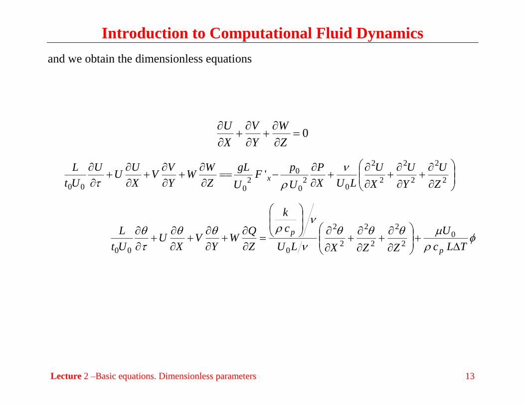
Lecture 2 –Basic equations. Dimensionless parameters 13
and we obtain the dimensionless equations
0
Z
W
Y
V
X
U
2
2
2
2
2
2
02
0
02
000
'Z
U
Y
U
X
U
LUX
P
U
pF
U
gL
Z
WW
Y
VV
X
UU
U
Ut
Lx
TLc
U
ZZXLU
c
k
Z
QW
YV
XU
Ut
L
p
p
02
2
2
2
2
2
000

Introduction to Computational Fluid Dynamics
Lecture 2 –Basic equations. Dimensionless parameters 14
Dimensionless numbers
A. Strouhal number
The Strouhal number (St) is a dimensionless number describing oscillating flow
mechanisms:
velocityaverage
noscillatio
U
L
Ut
LSt
000
B. Froude number
The Froude number (Fr) is a dimensionless number defined as the ratio of the flow inertia
to the external field (the latter in many applications simply due to gravity).
In naval architecture the Froude number is a very significant figure used to determine the
resistance of a partially submerged object moving through water, and permits the
comparison of similar objects of different sizes, because the wave pattern generated is
similar at the same Froude number only.
gL
UFr 0

Introduction to Computational Fluid Dynamics
Lecture 2 –Basic equations. Dimensionless parameters 15
C. Euler number
It expresses the relationship between a local pressure drop e.g. over a restriction and the
kinetic energy per volume, and is used to characterize losses in the flow, where a perfect
frictionless flow corresponds to an Euler number of 1.
20
0
U
pEu
Usually, we take 2
00 Up and we obtain Eu = 1.
D. Reynolds number
LULU 00Re
The Reynolds number is defined as the ratio of inertial forces to viscous forces and
consequently quantifies the relative importance of these two types of forces for given
flow conditions.
laminar flow occurs at low Reynolds numbers, where viscous forces are dominant,
and is characterized by smooth, constant fluid motion;
turbulent flow occurs at high Reynolds numbers and is dominated by inertial forces,
which tend to produce chaotic eddies, vortices and other flow instabilities.

Introduction to Computational Fluid Dynamics
Lecture 2 –Basic equations. Dimensionless parameters 16
E. Prandtl number
p
p
ckk
cPr
/
/
It is the ratio of momentum diffusivity to thermal diffusivity. The Prandtl number
contains no such length scale in its definition and is dependent only on the fluid and the
fluid state. As such, the Prandtl number is often found in property tables alongside other
properties such as viscosity and thermal conductivity.
•gases - Pr ranges 0.7 - 1.0 •water - Pr ranges 1 - 10
•liquid metals - Pr ranges 0.001 - 0.03 •oils - Pr ranges 50 - 2000
E. Eckert number
It expresses the relationship between a flow's kinetic energy and the boundary layer
enthalpy difference, and is used to characterize heat dissipation.
Tc
UΕc
p
20

Introduction to Computational Fluid Dynamics
Lecture 2 –Basic equations. Dimensionless parameters 17
Using the above dimensionless numbers we obtain:
0
Z
W
Y
V
X
U
2
2
2
2
2
2
Re
1'
1
Z
U
Y
U
X
U
X
PEuF
FrZ
WW
Y
VV
X
UU
USt x
….
RePrRe
12
2
2
2
2
2 Ec
ZZXZ
QW
YV
XUSt
or using differential operators
0 V
(23)
VRe
PEuFFr
VVV
St
1'
1
(24)
Re
Ec
PrReVSt
1 (25)

Introduction to Computational Fluid Dynamics
Lecture 2 –Basic equations. Dimensionless parameters 18
Comments
Dimensionless numbers allow for comparisons between very different systems and
tell you how the system will behave
Many useful relationships exist between dimensionless numbers that tell you how
specific things influence the system
When you need to solve a problem numerically, dimensionless groups help you to
scale your problem.
Analytical studies can be performed for limiting values of the dimensionless
parameters
Express the governing equations in dimensionless form to:
(1) identify the governing parameters
(2) plan experiments
(3) guide in the presentation of experimental results and theoretical solutions
If the flow is not oscillatory, we take usually 00 ULt and thus St =1. If 0t we have
St = 0 and the flow is steady.

Introduction to Computational Fluid Dynamics
Lecture 2 –Basic equations. Dimensionless parameters 19
Numerical methods for initial values problems (IVP or Cauchy problem)
Pendulum
Radioactive elements decay:
mdt
dm , 00)( mtm
where m is the mass of the radioactive element and is the decay constant.
L
Mathematical model:
0sin2
2
L
g
dt
d, 0000 ')(,)(
t
dt
dt

Introduction to Computational Fluid Dynamics
Lecture 2 –Basic equations. Dimensionless parameters 20
Theoretical aspects
The general Cauchy problem:
ayay
btaytfty
)(
),,()('
Using numerical methods we obtain a discrete approximation of y in
some points, called nodes, which form a grid (mesh).
A grid for the interval ],[ ba having a constant step h is:
bhNaihahahaa ,)1(,...,...,,2,,
or
Nihiati ...,,1,)1(
where N is the number of subintervals, and the step is constant:
)1/()( Nabh .

Introduction to Computational Fluid Dynamics
Lecture 2 –Basic equations. Dimensionless parameters 21
By using a numerical method we obtain the approximated discrete values
Niyty i
not
i ...,,1,)(
t
yi-2
i-2
yi-1 yi
yi+1 yi+2
i-1 i i+1 i+2
y(t)

Introduction to Computational Fluid Dynamics
Lecture 2 –Basic equations. Dimensionless parameters 22
One step methods
An example: The Euler method (Leonhard Euler-(1707 – 1783))
ayay
btaytfty
)(
),,()('
By using a Taylor expansion (y should be of
class 2C ) we have:
),(),("2
)(')()()( 1
2
1 iiiiiiii ttyh
tyhtyhtyty
Thus, one get:
))(,()()( 1 iiii tytfhtyty )("2
2
iyh
By dropping the last term the Euler formula is obtained:
1...,,1,0),,(1
0
Niytfhyy
yy
iiii
a
Remark: 1i
y depends on iy , it and h.

Introduction to Computational Fluid Dynamics
Lecture 2 –Basic equations. Dimensionless parameters 23
(Richard L. Burden and J. Douglas Faires , Numerical Analysis,Ninth Edition, 2011).

Introduction to Computational Fluid Dynamics
Lecture 2 –Basic equations. Dimensionless parameters 24
One may notice that the
Euler method follow the
tangent for the current
node to approximate the
value in the next node.

Introduction to Computational Fluid Dynamics
Lecture 2 –Basic equations. Dimensionless parameters 25
Same problem for h = 0.2 (11 nodes). Comparison with the

Introduction to Computational Fluid Dynamics
Lecture 2 –Basic equations. Dimensionless parameters 26
An one step method for the Cauchy problem is given by
nn
niiii
ba
hbaythythyy
RR
R
1
1
],[:
0,],[],[),,,(
Considering the exact solution (in the grid points) )(~ity we define the
local truncation error as follow:
h
tytyhyt
h
tyty
h
yyhytT ii
iiiiii
ii
)(~)(~),,(
)(~)(~),,( 111
(the difference between the approximation increment and the exact increment for one step)
A method is consistent if 0),,( hytT uniformly when 0h for nbayt R ],[),( .
(it is necessary that ),()0,,( ytfyt )

Introduction to Computational Fluid Dynamics
Lecture 2 –Basic equations. Dimensionless parameters 27
A method is of order p if
pKhhytT ),,(
uniformly on nba R],[ , where is a vector norm, and K is constant.
We may use the following notation:
0),(),,( hhOhytT p
(for 1p the method is consistent).
It can be shown that Euler method is a method of order one, )(hO .

Introduction to Computational Fluid Dynamics
Lecture 2 –Basic equations. Dimensionless parameters 28
Improved Euler methods
evaluation of the tangent is made in an intermediary point of the interval 1, ii tt
ti ti+1 ti+1/2
yEuler
ymodified
yexact
y(t)
t
ti ti+1
yi
slope = f(ti, yi)
slope = f(ti+1, yi+hf(ti, yi))
average slope
Modified Euler
Heun
Introduction to Computational Fluid Dynamics
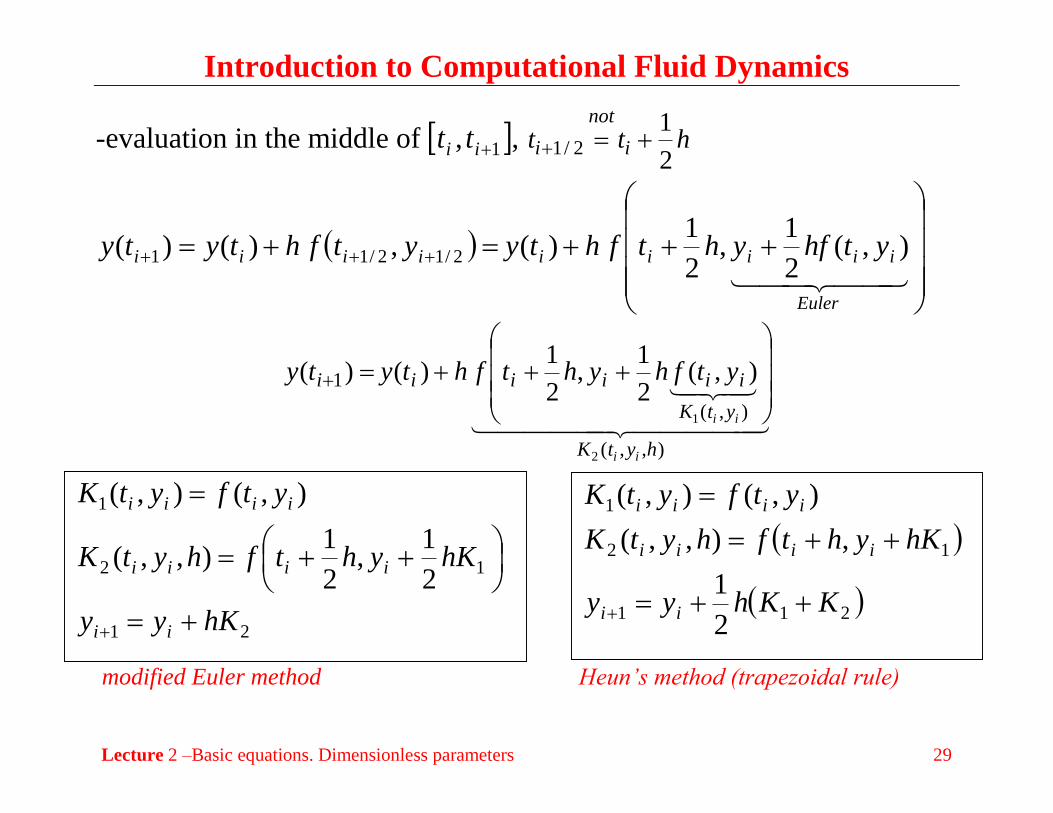
Lecture 2 –Basic equations. Dimensionless parameters 29
-evaluation in the middle of 1, ii tt , htt i
not
i2
12/1
Euler
iiiiiiiii ythfyhtfhtyytfhtyty ),(2
1,
2
1)(,)()( 2/12/11
),,(
),(
1
2
1
),(2
1,
2
1)()(
hytK
ytK
iiiiii
ii
ii
ytfhyhtfhtyty
modified Euler method Heun’s method (trapezoidal rule)
21
12
1
2
1,
2
1),,(
),(),(
hKyy
hKyhtfhytK
ytfytK
ii
iiii
iiii
211
12
1
2
1
,),,(
),(),(
KKhyy
hKyhtfhytK
ytfytK
ii
iiii
iiii

Introduction to Computational Fluid Dynamics
Lecture 2 –Basic equations. Dimensionless parameters 30
Runge-Kutta type methods
evaluation in intermediary points of 1, ii tt
Carl David Tolmé Runge Martin Wilhelm Kutta
(1856 – 1927) (1867 – 1944)
Standard Runge-Kutta method
43211 226
KKKKh
yy ii
34
23
2
1
,
2
1,
2
1
12
1,
2
1
),(
hKyhtfK
hKyhtfK
hKyhtfK
ytfK
ii
ii
ii
ii

Introduction to Computational Fluid Dynamics
Lecture 2 –Basic equations. Dimensionless parameters 31
Matlab solvers for Cauchy problems (ODE)
Syntax
[t,Y] = solver(odefun,tspan,y0,options, p1, p2, ...)
or
sol = solver(odefun,[t0 tf],y0...)
where solver can be
ode45, ode23, ode113, ode15s, ode23s, ode23t or ode23tb.
Input parameters (selection)
odefun – right hand member of the Cauchy problem
tspan –integration interval.
y0– initial value
options – solver options.

Introduction to Computational Fluid Dynamics
Lecture 2 –Basic equations. Dimensionless parameters 32
Output parameters:
t – column vector of time points;
y – solution array
sol – solution structure

Introduction to Computational Fluid Dynamics
Lecture 2 –Basic equations. Dimensionless parameters 33

Introduction to Computational Fluid Dynamics
Lecture 2 –Basic equations. Dimensionless parameters 34
Example: Solve pendulum equation using ode45:
0sin2
2
L
g
dt
d, 1.0)0(,0)0(
dt
d
We note 1y and rewrite the system in the form
1.00;00
sin
;
11
12
21
dt
dyy
yL
g
dt
dy
ydt
dy
function dy=fPendul(t,y,flag,g,L)
dy=[y(2);-g/L*sin(y(1))];

Introduction to Computational Fluid Dynamics
Lecture 2 –Basic equations. Dimensionless parameters 35
%pendulum equation
a=0;b=pi/2;%integration interval
g=9.8;%accelaration due to the gravity
L=0.1;%length of the pendulum
y0=[0,0.1];%initial conditions
options=odeset('RelTol',1e-8);%modify the options
%use the solver
[t,y]=ode45('fPendul',[a,b],y0,options,g,L)
plot(t,y(:,1));