Embed Size (px)
Citation preview

Introduction to Bayesian thinking
Statistics seminar
Rodrigo Díaz
Geneva Observatory, April 11th, 2016

Agenda (I)
• Part I. Basics.
• General concepts & history of Bayesian statistics.
• Bayesian inference.
• Part II. Likelihoods.
• Constructing likelihoods.
• Part III. Priors.
• General concepts and problems. Subjective vs objective priors.
• Assigning priors.

Agenda (II)
• Part IV. Posterior.
• Conjugate priors. The right prior for a given likelihood.
• MCMC.
• Part V. Model comparison.
• Model evidence and Bayes factor. The philosophy of integrating over parameter space.
• Estimating the model evidence. Dos and Don’ts
• Point estimate: BIC.
• Importance sampling and a family of methods.
• Nested sampling.

Part I basics

Statistical inferenceFig. adapted from Gregory (2005)
Observations (data)
Testable hypothesis
(theory)
Deductive inference (predictions)
Statistical inference (hyp. testing,
parameter estimation)

Statistical inferencerequires a probability theory
Frequentist
Bayesian

Thomas Bayes (1701 – 1761)First appearance of the product rule (the base for the Bayes’ theorem; An Essay towards solving a Problem in the Doctrine of Chances).
Pierre-Simon Laplace (1749 – 1827)Wide application of the Bayes' rule. Principle of insufficient reason (non-informative priors). Primitive version of the Bernstein–von Mises theorem.
Laplace’s “inverse probability” is largely rejected for ~100 years. The reign of frequentist probability. Fischer, Pearson, etc.
p(Hi|I,D) = p(D|Hi,I)p(D|I) · p(Hi|I)

Harold Jeffreys (1891 – 1989)Objective Bayesian probability revived. Jeffreys rule for priors.
(1940s - 1960s) R. T. Cox George Pólya E. T. JaynesPlausible reasoning. Reasoning with uncertainty. Probability theory as an extension of Aristotelian logic. The product and sum rules deduced for basic principles. MAXENT priors.
See E.T Jaynes. Probability Theory: The Logic of Science. http://www-biba.inrialpes.fr/Jaynes/prob.html

Statistical inferenceFig. adapted from Gregory (2005)
Observations (data)
Testable hypothesis
(theory)
Deductive inference (predictions)
Statistical inference (hyp. testing,
parameter estimation)

The three desiderata
• Rules of deductive reasoning: strong syllogisms from Aristotelian logic.• Brain works using plausible inference. Woman in wood cabin story.• The rules for plausible reasoning are deduced from three simple
desiderata on how the mind of a thinking robot should work (Cox-Póyla-Jaynes).
I. Degrees of Plausibility are represented by real numbers.
II. Qualitative Correspondence with common sense.III. If a conclusion can be reasoned out in more than
one way; then every possible way must lead to the same result.

“… if degrees of plausibility are represented by real numbers ︎, then there is a uniquely determined set of quantitative rules for conducting inference ︎ That is ︎ any, other rules whose results conflict with them will necessarily violate an elementary -and nearly inescapable- desideratum of rationality or consistency.
But the final result was just the standard rules of probability theory, given already by Bernoulli and Laplace, so why all the fuss? The important new feature was that these rules were now seen as uniquely valid principles of logic in general, making no reference to “chance” or “random variables”; so their range of application is vastly greater than had been supposed in the conventional probability theory that was developed in the early 20th century. As a result, the imaginary distinction between ︎probability theory︎ and ︎statistical inference︎ disappears ︎ and the field achieves not only logical unity and simplicity ︎ but far greater technical power and flexibility in applications.”

The basic rules of probability theory.
p(A+B) = p(A) + p(B)� p(AB)
p(AB) = p(A|B)p(B) = p(B|A)p(A)
A BSum
Product“Aristotelian
deductive logic is the
limiting form of our rules
for plausible reasoning”
E.T. Jaynes
Once these rules are recognised as general ways of manipulating any preposition, a world of applications opens up.

“… if degrees of plausibility are represented by real numbers ︎, then there is a uniquely determined set of quantitative rules for conducting inference ︎ That is ︎ any, other rules whose results conflict with them will necessarily violate an elementary -and nearly inescapable- desideratum of rationality or consistency.
But the final result was just the standard rules of probability theory, given already by Bernoulli and Laplace, so why all the fuss? The important new feature was that these rules were now seen as uniquely valid principles of logic in general, making no reference to “chance” or “random variables”; so their range of application is vastly greater than had been supposed in the conventional probability theory that was developed in the early 20th century. As a result, the imaginary distinction between ︎probability theory︎ and ︎statistical inference︎ disappears ︎ and the field achieves not only logical unity and simplicity ︎ but far greater technical power and flexibility in applications.”

Bayes’ theorem
p(A|B) =p(B|A) p(A)
p(B)
The Bayesian recipe
p(AB) = p(A|B)p(B) = p(B|A)p(A)Product
p(A+B) = p(A) + p(B)� p(AB)Sum

The Bayesian recipe
Law of Total Probability
for {Bi} exclusive and exhaustive
B5
B4B1
B2 B3
B6
A
p(A|I) =X
i
p(A|Bi, I)p(Bi|I)

Bayes’ theorem
p(A|B) =p(B|A) p(A)
p(B)
The Bayesian recipe
p(AB) = p(A|B)p(B) = p(B|A)p(A)Product
p(A+B) = p(A) + p(B)� p(AB)Sum
Law of Total Probability
for {Bi} exclusive and exhaustive
p(A|I) =X
i
p(A|Bi, I)p(Bi|I)

Bayes’ theorem
p(A|B) =p(B|A) p(A)
p(B)
The Bayesian recipe
p(AB) = p(A|B)p(B) = p(B|A)p(A)Product
p(A+B) = p(A) + p(B)� p(AB)Sum
Law of Total Probability
for {Bi} exclusive and exhaustive
p(A|I) =X
i
p(A|Bi, I)p(Bi|I)
Normalisation
X
i
p(Bi|I) = 1for {Bi} exclusive and exhaustive

"Bayes", "Bayesian", MCMC


Two basic tasks of statistical inference
Learning process (parameter estimation)
Decision making (model comparison)

Bayesian probability represents a state of knowledge
Learning process
p(Hi|I) p(Hi|I,D)
D: data Discrete space (hypothesis space)
Posteriorp(✓̄|D,Hi, I)p(✓̄|Hi, I)
Prior: parameter vector Hi: hypothesis I: information
✓̄
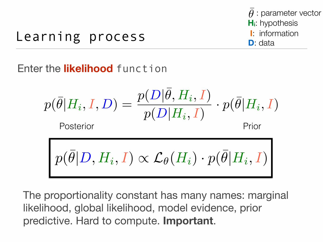
Enter the likelihood function
Learning process
p(✓̄|Hi, I,D) =p(D|✓̄, Hi, I)
p(D|Hi, I)· p(✓̄|Hi, I)
PriorPosterior
D: data
: parameter vector Hi: hypothesis I: information
✓̄
p(✓̄|D,Hi, I) / L✓(Hi) · p(✓̄|Hi, I)
The proportionality constant has many names: marginal likelihood, global likelihood, model evidence, prior predictive. Hard to compute. Important.

Optimising the learning process
• The likelihood needs to be selective for the learning process to be effective.
Two extreme cases are shown in Figure 1.2. In the first, panel (a), the prior is
much broader than the likelihood. In this case, the posterior PDF is determinedentirely by the new data. In the second extreme, panel (b), the new data are much
less selective than our prior information and hence the posterior is essentially theprior.
Now suppose we acquire more data represented by proposition D2. We can againapply Bayes’ theorem to compute a posterior that reflects our new state of knowledge
about the parameter. This time our new prior, I 0, is the posterior derived from D1; I,i.e., I 0 ¼D1; I. The new posterior is given by
pðH0jD2; I0Þ / pðH0jI 0ÞpðD2jH0; I
0Þ: (1:13)
1.3.4 Example of the use of Bayes’ theorem
Here we analyze a simple model comparison problem using Bayes’ theorem. We startby stating our prior information, I, and the new data, D.
I stands for:
a) Model M1 predicts a star’s distance, d1 ¼ 100 light years (ly).
b) Model M2 predicts a star’s distance, d2 ¼ 200 ly.
c) The uncertainty, e, in distance measurements is described by a Gaussian distribution of
the form
Parameter H0
(a)
Posteriorp(H0|D,M1,I )
Likelihoodp(D |H0,M1,I )
Priorp(H0|M1,I )
Parameter H0
(b)
Posteriorp(H0|D,M1,I )
Priorp(H0|M1,I )
Likelihoodp(D |H0,M1,I )
Figure 1.2 Bayes’ theorem provides a model of the inductive learning process. The posteriorPDF (lower graphs) is proportional to the product of the prior PDF and the likelihood function(upper graphs). This figure illustrates two extreme cases: (a) the prior much broader thanlikelihood, and (b) likelihood much broader than prior.
8 Role of probability theory in science
P. Gregory (2005)
Domina
ted
by prio
r
inform
ation
Dominated
by data

Bayes’ theorem is also the base for model comparison
Computation of the evidence cannot be escaped.
but now
p(Hi|I,D) =p(D|Hi, I)
p(D|I) · p(Hi|I)
p(D|Hi, I) =
Z
⇡p(D|✓̄, Hi, I)p(✓̄|Hi, I) d
n✓
Decision making

Model comparison consists in computing the ratio of the posteriors (odds ratio) of two competing hypotheses.
Bayes factor Prior odds
p(Hi|I)
p(Hi|I,D)
p(D|Hi, I)
p(Hi|I,D) =p(D|Hi, I)
p(D|I)· p(Hi|I)
D = DRVDtransitDastrometry...DN
p(D|H, I) = p(E1, E2, ..., EN |H, I)indep.=
N∏
i=1
p(Ei|H, I)
L(Hi) = p(D|θ̄, Hi, I)indep.,gauss.
∝ exp−χ2θ̄
2
p(Hi|D, I)
p(Hj |D, I)
p(θ̄|Hi, I,D) =p(D|θ̄, Hi, I)
p(D|Hi, I)· p(θ̄|Hi, I)
p(θ̄|Hi, I)
p(θ̄|D,Hi, I) ∝ p(D|θ̄, Hi, I) · p(θ̄|Hi, I)
p(θ̄|D,Hi, I) ∝ L(Hi) · p(θ̄|Hi, I)
p(Hi|D, I) ∝ p(D|Hi, I) · p(Hi|I)
p(Hi|I,D)
p(Hj |I,D)∝
p(D|Hi, I)
p(D|Hj , I)·p(Hi|I)
p(Hj |I)
1
p(Hi|I,D)p(Hj |I,D) =
p(D|Hi,I)p(D|Hj ,I)
· p(Hi|I)p(Hj |I)
Decision making
Part II likelihoods

The likelihood function
p(✓̄|Hi, I,D) =p(D|✓̄, Hi, I)
p(D|Hi, I)· p(✓̄|Hi, I)
PriorPosterior
D: data
: parameter vector Hi: hypothesis I: information
✓̄
p(✓̄|D,Hi, I) / L✓(Hi) · p(✓̄|Hi, I)
The likelihood is the probability of obtaining data D, for a given prior information I and a set of parameters !.
Remember, likelihood is not a probability for parameter vector !(for that you need the prior)

Optimising the learning process
• The likelihood needs to be selective for the learning process to be effective.
Two extreme cases are shown in Figure 1.2. In the first, panel (a), the prior is
much broader than the likelihood. In this case, the posterior PDF is determinedentirely by the new data. In the second extreme, panel (b), the new data are much
less selective than our prior information and hence the posterior is essentially theprior.
Now suppose we acquire more data represented by proposition D2. We can againapply Bayes’ theorem to compute a posterior that reflects our new state of knowledge
about the parameter. This time our new prior, I 0, is the posterior derived from D1; I,i.e., I 0 ¼D1; I. The new posterior is given by
pðH0jD2; I0Þ / pðH0jI 0ÞpðD2jH0; I
0Þ: (1:13)
1.3.4 Example of the use of Bayes’ theorem
Here we analyze a simple model comparison problem using Bayes’ theorem. We startby stating our prior information, I, and the new data, D.
I stands for:
a) Model M1 predicts a star’s distance, d1 ¼ 100 light years (ly).
b) Model M2 predicts a star’s distance, d2 ¼ 200 ly.
c) The uncertainty, e, in distance measurements is described by a Gaussian distribution of
the form
Parameter H0
(a)
Posteriorp(H0|D,M1,I )
Likelihoodp(D |H0,M1,I )
Priorp(H0|M1,I )
Parameter H0
(b)
Posteriorp(H0|D,M1,I )
Priorp(H0|M1,I )
Likelihoodp(D |H0,M1,I )
Figure 1.2 Bayes’ theorem provides a model of the inductive learning process. The posteriorPDF (lower graphs) is proportional to the product of the prior PDF and the likelihood function(upper graphs). This figure illustrates two extreme cases: (a) the prior much broader thanlikelihood, and (b) likelihood much broader than prior.
8 Role of probability theory in science
Two extreme cases are shown in Figure 1.2. In the first, panel (a), the prior is
much broader than the likelihood. In this case, the posterior PDF is determinedentirely by the new data. In the second extreme, panel (b), the new data are much
less selective than our prior information and hence the posterior is essentially theprior.
Now suppose we acquire more data represented by proposition D2. We can againapply Bayes’ theorem to compute a posterior that reflects our new state of knowledge
about the parameter. This time our new prior, I 0, is the posterior derived from D1; I,i.e., I 0 ¼D1; I. The new posterior is given by
pðH0jD2; I0Þ / pðH0jI 0ÞpðD2jH0; I
0Þ: (1:13)
1.3.4 Example of the use of Bayes’ theorem
Here we analyze a simple model comparison problem using Bayes’ theorem. We startby stating our prior information, I, and the new data, D.
I stands for:
a) Model M1 predicts a star’s distance, d1 ¼ 100 light years (ly).
b) Model M2 predicts a star’s distance, d2 ¼ 200 ly.
c) The uncertainty, e, in distance measurements is described by a Gaussian distribution of
the form
Parameter H0
(a)
Posteriorp(H0|D,M1,I )
Likelihoodp(D |H0,M1,I )
Priorp(H0|M1,I )
Parameter H0
(b)
Posteriorp(H0|D,M1,I )
Priorp(H0|M1,I )
Likelihoodp(D |H0,M1,I )
Figure 1.2 Bayes’ theorem provides a model of the inductive learning process. The posteriorPDF (lower graphs) is proportional to the product of the prior PDF and the likelihood function(upper graphs). This figure illustrates two extreme cases: (a) the prior much broader thanlikelihood, and (b) likelihood much broader than prior.
8 Role of probability theory in science
P. Gregory (2005)
Domina
ted
by prio
r
inform
ation
Dominated
by data
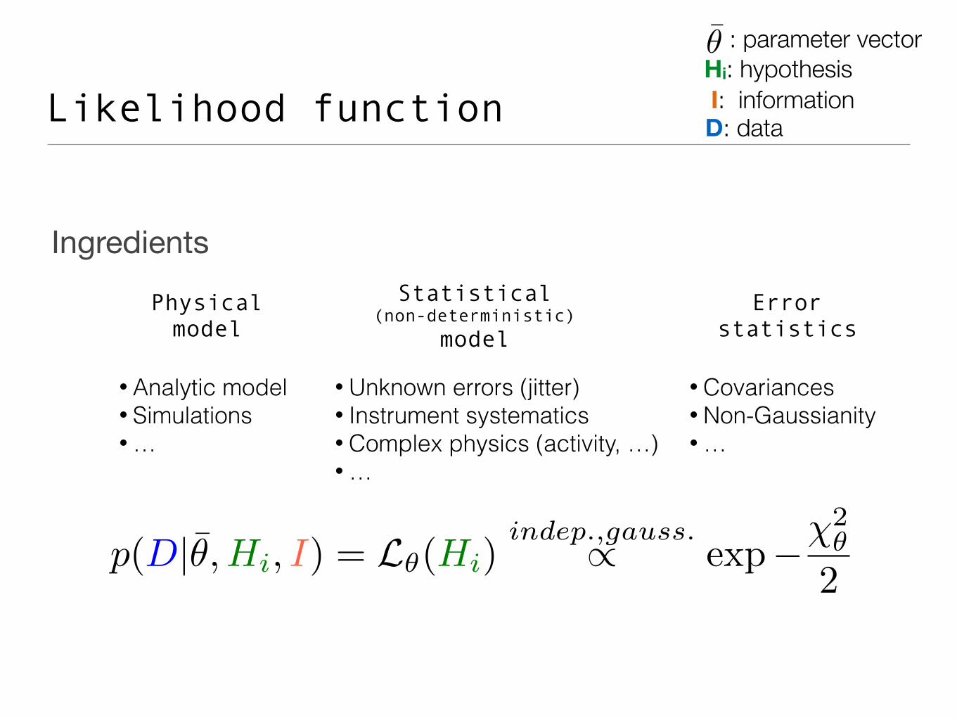
Ingredients
Likelihood function D: data
: parameter vector Hi: hypothesis I: information
✓̄
Statistical (non-deterministic)
model
Physical model
Error statistics
• Analytic model • Simulations • …
• Unknown errors (jitter) • Instrument systematics • Complex physics (activity, …) • …
• Covariances • Non-Gaussianity • …
p(D|¯✓, Hi, I) = L✓(Hi)indep.,gauss./ exp��2
✓
2

Constructing the likelihood
D = D1 D2 ... Dn = {Di}Di: the i-th measurement is in the infinitesimal range yi to yi + dyi
The data:
The errors:
Ei: the i-th error is in the infinitesimal range ei to ei + dei
p(Ei|✓, H, I) = fE(ei) The probability distribution of statement Ei
Most used fEfE(ei) = N(0,�2
i )
The model:
Mi: the i-th error is in the infinitesimal range mi to mi + dmi
p(Mi|✓, H, I) = fM (mi) The probability distribution of statement Mi

Constructing the likelihood
D = D1 D2 ... Dn = {Di}The data:
yi = mi + eiWrite:
p(D|✓, H, I) = p(D1, D2, ..., Dn|✓, H, I)
We want to build the probability distribution:
p(Di|✓, H, I) =
Zdmi fM (mi) fE(yi �mi)
It can be shown that: Convolution
equation

Constructing the likelihood
p(Di|✓, H, I) =
Zdmi fM (mi) fE(yi �mi)
But for a deterministic model, mi is obtained from a (usually analytically) function f without any uncertainty (say, a Keplerian curve for RV measurements)
mi = f(xi|✓)fM (mi) = �(mi � f(xi|✓))
Then: p(Di|✓, H, I) =
Zdmi �(mi � f(xi|✓)) fE(yi �mi)
= fE(yi � f(xi|✓) = p(Ei|✓, H, I)
p(D|✓, H, I) = p(D1, D2, ..., Dn|✓, H, I) = p(E1, E2, ..., En|✓, H, I)
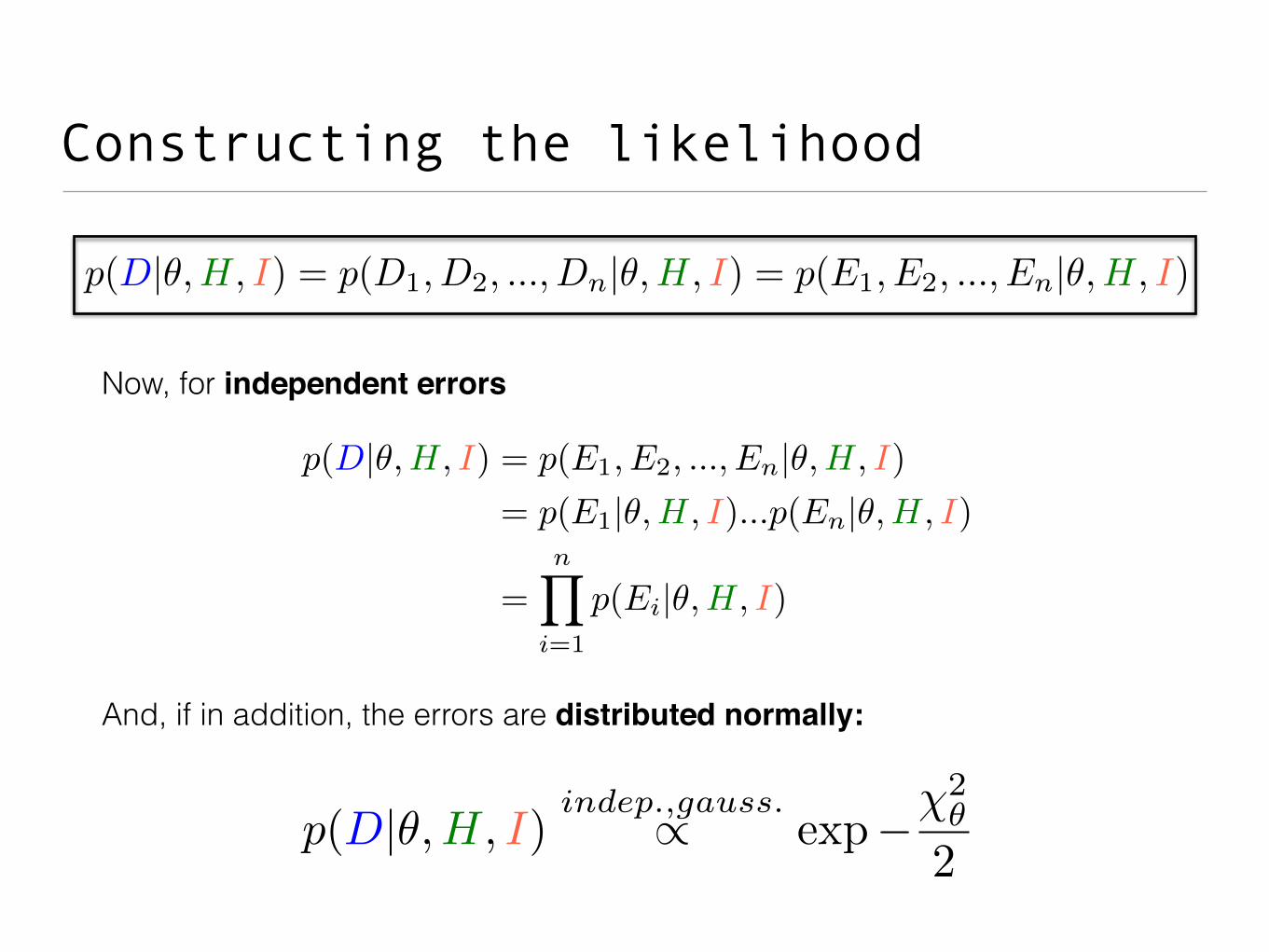
Constructing the likelihood
Now, for independent errors
p(D|✓, H, I) = p(D1, D2, ..., Dn|✓, H, I) = p(E1, E2, ..., En|✓, H, I)
p(D|✓, H, I) = p(E1, E2, ..., En|✓, H, I)
= p(E1|✓, H, I)...p(En|✓, H, I)
=nY
i=1
p(Ei|✓, H, I)
And, if in addition, the errors are distributed normally:
p(D|✓, H, I)indep.,gauss./ exp��2
✓
2

Constructing the likelihood
p(Di|✓, H, I) =
Zdmi fM (mi) fE(yi �mi)
For a non-deterministic model, Mi is distributed:
Back to the convolution equation
Mi: the i-th error is in the infinitesimal range mi to mi + dmi
p(Mi|✓, H, I) = fM (mi) The probability distribution of statement Mi
E.g. adding instrumental error / resolution:
fM (mi) = N(f(xi|✓),�2inst)

Part III priors

Prior probabilities
Hi: hypothesis (can be continuous). I: information
• Prior information I is always present:
• The term “prior” does not necessarily mean “earlier in time”.
• Philosophical controversy on how to assign priors.
• Subjective vs. objective views.
• No single universal rule, but a few accepted methods.
• Informative priors. Usually based on the output from previous observations. (What was the prior of the first analysis?).
• Ignorance priors. Required as a starting point for the theory.
p(Hi|I)

Assigning ignorance priors
1. Principle of indifference.
Given n mutually exclusive, exhaustive hypothesis, {Hi}, with i = 1, …, n, the PoI states:
p(Hi|I) = 1/n

Assigning ignorance priors
2. Transformation groups. Location and scale parameters.
For a certain type of parameters (location and scale), “total ignorance” can we represented as invariance under certain (group of) transformation.
Location: “position of highest tree along a river.” Problem must be invariant under a translation.
X 0 = X + c
p(X|I) dX = p(X 0|I) dX 0 =
p(X 0|I)d(X + c) = p(X 0|I)dX
p(X|I) = constant
Uniform prior.

Assigning ignorance priors
2. Transformation groups. Location and scale parameters.
For a certain type of parameters (location and scale), “total ignorance” can we represented as invariance under certain (group of) transformation.
Scale: “life time of a new bacteria” or “Poisson rate” Problem must be invariant under scaling.
“Jeffreys” prior.
X 0 = aX
p(X|I) dX = p(X 0|I) dX 0 =
p(X 0|I)d(aX) = ap(X 0|I)dX
p(X|I) = constant
x

3. Jeffreys rule.
Besides location and scale parameters, little more can be said using transformation invariance.
Jeffreys priors use the Fisher information; parameterisation invariant, but strange behaviour in many dimensions.
Assigning ignorance priors
Observed Fischer information: ID = �d
2logLD
d✓2
But D is not known when we have to define a prior. Use expectation value over D.
I(✓) = �ED
d
2logLD
d✓2
�

3. Jeffreys rule says:
Assigning ignorance priors
p(✓|I) /p
I(✓)
Examples:
• Mean of Normal distribution (") with known variance #^2.
• Rate $ of Poisson distribution.
• Exercise: Scale of Normal with known mean value?
p(µ|�2, I) / constant
p(�|I) / 1/p�

3. Jeffreys rule:
Assigning ignorance priors
p(✓|I) /p
I(✓)
• Favours parts of parameter space where data provides more information.
• Is invariant under reparametrisation.
• Works fine only in one dimension…
See more examples here: en.wikipedia.org/wiki/Jeffreys_prior
I(✓) = �ED
d
2logLD
d✓2
�

Assigning ignorance priors
4. Maximum entropy.
Uses information theory to define a measurement of the distribution information.
S = �nX
i=0
pi log(pi)
• Maximise entropy subject to constraints (use Lagrange multipliers).
• Defined strictly for discrete distributions.
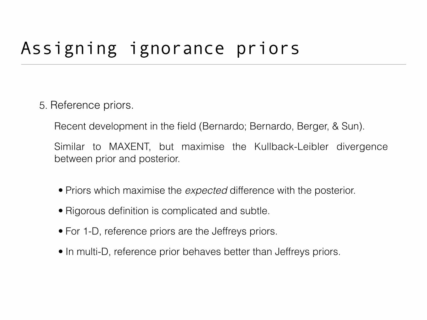
Assigning ignorance priors
5. Reference priors.
Recent development in the field (Bernardo; Bernardo, Berger, & Sun).
Similar to MAXENT, but maximise the Kullback-Leibler divergence between prior and posterior.
• Priors which maximise the expected difference with the posterior.
• Rigorous definition is complicated and subtle.
• For 1-D, reference priors are the Jeffreys priors.
• In multi-D, reference prior behaves better than Jeffreys priors.

Agenda (II)
• Part IV. Posterior.
• Conjugate priors. The right prior for a given likelihood.
• MCMC.
• Part V. Model comparison.
• Model evidence and Bayes factor. The philosophy of integrating over parameter space.
• Estimating the model evidence. Dos and Don’ts
• BIC, Chib & Jeliazkov, etc.
• Importance sampling and a family of methods.

Part IV sampling the posterior / MCMC

Sampling from the posterior
p(✓̄|D,Hi, I) / L✓(Hi) · p(✓̄|Hi, I)
• The posterior distribution is proportional to the likelihood times the prior.
• The normalising constant (called model evidence, marginal likelihood, etc.) is of importance when comparing different models.
• The posterior contains all the information on a given model a Bayesian statistician can get for a given set of priors and data.
• Posterior is only analytical in few cases:
• Conjugate priors.
• Other methods needed to sample from posterior.
Remember, most Bayesian computations can be reduced to expectation values with respect to the posterior.

Markov Chain Monte Carlo D: data
: parameter vector Hi: hypothesis I: information
✓̄
Metropolis-Hastings
p(✓̄|D,Hi, I) / L✓(Hi) · p(✓̄|Hi, I)
✓̄0*
✓̄0*q(✓̄ 0, ✓̄)
L✓0 · p(✓̄0|I)1.
2. Create proposal point.
L✓0 · p(✓̄0|I)3.
r = L✓0 ·p(✓̄0|I)L✓0 ·p(✓̄0|I)
4.

Markov Chain Monte Carlo D: data
: parameter vector Hi: hypothesis I: information
✓̄
Metropolis-Hastings
p(✓̄|D,Hi, I) / L✓(Hi) · p(✓̄|Hi, I)
L✓0 · p(✓̄0|I)1.
2. Create proposal point.
L✓0 · p(✓̄0|I)3.
r = L✓0 ·p(✓̄0|I)L✓0 ·p(✓̄0|I)
4.
5. Accept proposal with probability min(1, r)
✓̄0 q(✓̄0 , ✓̄)
*
✓̄0*
*q(✓̄ 0, ✓̄)
✓̄1

Markov Chain Monte Carlo D: data
: parameter vector Hi: hypothesis I: information
✓̄
Metropolis-Hastings
p(✓̄|D,Hi, I) / L✓(Hi) · p(✓̄|Hi, I)
L✓0 · p(✓̄0|I)1.
2. Create proposal point.
L✓0 · p(✓̄0|I)3.
r = L✓0 ·p(✓̄0|I)L✓0 ·p(✓̄0|I)
4.
5. Accept proposal with probability min(1, r)
✓̄0*
*
q(✓̄ 0, ✓̄)
✓̄1

Markov Chain Monte Carlo D: data
: parameter vector Hi: hypothesis I: information
✓̄
Metropolis-Hastings
p(✓̄|D,Hi, I) / L✓(Hi) · p(✓̄|Hi, I)
✓̄0 q(✓̄0 , ✓̄)
*
✓̄0*
*q(✓̄ 0, ✓̄)
✓̄1
pymc emcee kombine cobmcmc …
AlgorithmsMetropolis-Hastings Gibbs sampling Slice sampling … Hybrid Monte Carlo
Codes

5 minutes to LEARN
a lifetime to MASTER

But beware. Non-convergence,
bad mixing. The dark side of
MCMC are they.
Problems with correlations and multi-modal distributions.

The problem with Correlations
If parameters exhibit correlations, then step size must be small to reach the demanded fraction of accepted jumps.
Need a very long chain to explore the entire posterior. Or, more relevant, the entire posterior will not be explored thoroughly (i.e. reduced error bars!)
Rejected proposal
Accepted proposal

MCMC: the Good, the Bad, and the Ugly
Visual inspection of traces.
Good
Marginal mixing
No convergence

MCMC: the Good, the Bad, and the Ugly
Evaluation of the chain auto-correlations
Checking Autocorrelation Function
Image credit: E. Ford

Multi-modal posteriors.
Difficult for sampler to move across modes if separated by a low-probability barrier.
Has this Chain Converged?
Image credit: E. Ford

Multi-modal posteriors.
Run as many chains as possible starting from significantly different places in the prior space.
Be paranoid! You can always be missing modes.


Part V model comparison

Bayes’ theorem is also the base for model comparison
Computation of the model evidence (a.k.a. marginal likelihood, global likelihood, prior predictive, …) cannot be escaped.
but now
p(Hi|I,D) =p(D|Hi, I)
p(D|I) · p(Hi|I)
p(D|Hi, I) =
Z
⇡p(D|✓̄, Hi, I)p(✓̄|Hi, I) d
n✓
Decision making

Model comparison consists in computing the ratio of the posteriors (odds ratio) of two competing hypotheses.
Bayes factor Prior odds
p(Hi|I)
p(Hi|I,D)
p(D|Hi, I)
p(Hi|I,D) =p(D|Hi, I)
p(D|I)· p(Hi|I)
D = DRVDtransitDastrometry...DN
p(D|H, I) = p(E1, E2, ..., EN |H, I)indep.=
N∏
i=1
p(Ei|H, I)
L(Hi) = p(D|θ̄, Hi, I)indep.,gauss.
∝ exp−χ2θ̄
2
p(Hi|D, I)
p(Hj |D, I)
p(θ̄|Hi, I,D) =p(D|θ̄, Hi, I)
p(D|Hi, I)· p(θ̄|Hi, I)
p(θ̄|Hi, I)
p(θ̄|D,Hi, I) ∝ p(D|θ̄, Hi, I) · p(θ̄|Hi, I)
p(θ̄|D,Hi, I) ∝ L(Hi) · p(θ̄|Hi, I)
p(Hi|D, I) ∝ p(D|Hi, I) · p(Hi|I)
p(Hi|I,D)
p(Hj |I,D)∝
p(D|Hi, I)
p(D|Hj , I)·p(Hi|I)
p(Hj |I)
1
p(Hi|I,D)p(Hj |I,D) =
p(D|Hi,I)p(D|Hj ,I)
· p(Hi|I)p(Hj |I)
Decision making

A built-in Occam’s razor
The likelihood has a characteristic width2 which we represent by !". The character-istic width is defined by
Z
!"d" pðDj";M1; IÞ¼ pðDj"̂;M1; IÞ $ !": (3:21)
Then we can approximate the global likelihood (Equation (3.8)) for M1 in thefollowing way:
pðDjM1; IÞ¼Z
d" pð"jM1; IÞpðDj";M1; IÞ ¼ LðM1Þ
¼ 1
!"
Zd" pðDj";M1; IÞ
% pðDj"̂;M1; IÞ!"
!"
or alternatively; LðM1Þ % Lð"̂Þ !"!"
:
(3:22)
Since model M0 has no free parameters, no integral need be calculated to find itsglobal likelihood, which is simply equal to the likelihood for model M1 for " ¼ "0,
pðDjM0; IÞ¼ pðDj"0;M1; IÞ¼Lð"0Þ: (3:23)
Thus the Bayes factor in favor of the more complicated model is
B10 %pðDj"̂;M1; IÞpðDj"0;M1; IÞ
!"
!"¼ Lð"̂Þ
Lð"0Þ!"
!": (3:24)
Parameter θ
p(D|θ, M1, I ) = L(θ)
L(θ) = p(D|θ, M1, I )
p(θ|M1,I ) = 1∆θ
θ
δθ
∆θ
∧∧ ∧
Figure 3.1 The characteristic width !" of the likelihood peak and !" of the prior.
2 If the likelihood function is really a Gaussian and the prior is flat, it is simple to show that !" ¼ #"
ffiffiffiffiffiffi2p
p, where #" is the
standard deviation of the posterior PDF for ".
48 The how-to of Bayesian inference
Gregory (2005)
p(D|Hi, I) =
Zp(D|✓̄, Hi, I)p(✓̄|Hi, I) d✓̄
The Bayes factor naturally punishes models with more parameters
E.g.: model M0, without free parameters. Model M1, with one parameter.
M0 = M1(✓ = ✓0) p(D|M0, I) = p(D|✓0,M1, I)
p(D|M1, I) =
Zp(D|✓,M1, I) · p(✓|M1, I) d✓
=1
�✓
Zp(D|✓,M1, I) d✓
⇡ p(D|✓̂,M1, I)�✓
�✓
B10 ⇡ p(D|✓̂,M1, I)
p(D|✓0,M1, I)
�✓
�✓Occam’s factor One per parameter

Estimating the marginal likelihood
p(D|Hi, I) =
Z
⇡p(D|✓̄, Hi, I)p(✓̄|Hi, I) d
n✓
Marginal likelihood is a k-dimensional integral over parameter space.
Accounting for the “size” of parameter space bring many good things to Bayesian statistics, but the integral is intractable…
Large number of techniques to estimate the value of the integral:
• Asymptotic estimates (Laplace approximation, BIC).
• Importance sampling.
• Chib & Jeliazkov.
• Nested sampling.

Point Estimations
Information criteria for astrophysics L75
where the evidence is not readily calculable, and a simpler model
selection technique is required.
In this article I describe and apply an additional information cri-
terion, the Deviance Information Criterion (DIC) of Spiegelhalter
et al. (2002, henceforth SBCL02), which combines heritage from
both Bayesian methods and information theory. It has interesting
properties. First, unlike the AIC and BIC it accounts for the sit-
uation, common in astrophysics, where one or more parameters
or combination of parameters is poorly constrained by the data.
Secondly, it is readily calculable from posterior samples, such as
those generated by MCMC methods. It has already been used in
astrophysics to study quasar clustering (Porciani & Norberg 2006).
2 M O D E L S E L E C T I O N S TAT I S T I C S
2.1 Bayesian evidence
The Bayesian evidence, also known as the model likelihood and
sometimes, less accurately, as the marginal likelihood, comes from
a full implementation of Bayesian inference at the model level,
and is the probability of the data given the model. Using Bayes
theorem, it updates the prior model probability to the posterior model
probability. Usually the prior model probabilities are taken as equal,
but quoted results can readily be rescaled to allow for unequal ones if
required (e.g. Lasenby & Hobson 2006). In many circumstances the
evidence can be calculated without simplifying assumptions (though
perhaps with numerical errors). It has now been quite widely applied
in cosmology; see for example Jaffe (1996), Hobson, Bridle & Lahav
(2002), Saini, Weller & Bridle (2004), Trotta (2005), Parkinson et al.
(2006), and Lasenby & Hobson (2006).
The evidence is given by
E ≡
∫L(θ ) P(θ ) dθ, (1)
where θ is the vector of parameters being varied in the model and
P(θ ) is the properly normalized prior distribution of those parame-
ters (often chosen to be flat). It is the average value of the likelihood
L over the entire model parameter space that was allowed before
the data came in. It rewards a combination of data fit and model
predictiveness. Models which fit the data well and make narrow
predictions are likely to fit well over much of their available pa-
rameter space, giving a high average. Models which fit well for
particular parameter values, but were not very predictive, will fit
poorly in most of their parameter space, driving the average down.
Models which cannot fit the data well will do poorly in any event.
The integral in equation (1) may however be difficult to calculate,
as it may have too many dimensions to be amenable to evaluation
by gridding, and the simplest MCMC methods such as Metropolis–
Hastings produce samples only in the part of parameter space where
the posterior probability is high rather than throughout the prior.
Nevertheless, many methods exist (e.g. Gregory 2005; Trotta 2005),
and the nested sampling algorithm (Skilling 2006) has proven fea-
sible for many cosmology applications (Mukherjee et al. 2006;
Parkinson et al. 2006; Liddle et al. 2006b).
A particular property of the evidence worth noting is that it does
not penalize parameters (or, more generally, degenerate parameter
combinations) which are unconstrained by the data. If the likelihood
is flat or nearly flat in a particular direction, it simply factorizes out
of the evidence integral leaving it unchanged. This is an appealing
property, as it indicates that the model fitting the data is doing so
really by varying fewer parameters than at first seemed to be the
case, and it is the unnecessary parameters that should be discarded,
not the entire model.
2.2 AIC and BIC
Much of the literature, both in astrophysics and elsewhere, seeks a
simpler surrogate for the evidence which still encodes the tension
between fit and model complexity. In Liddle (2004), I described two
such statistics, the AIC and BIC, which have subsequently been quite
widely applied to astrophysics problems. They are relatively simple
to apply because they require only the maximum likelihood achiev-
able within a given model, rather than the likelihood throughout the
parameter space. Of course, such simplification comes at a cost, the
cost being that they are derived using various assumptions, partic-
ularly Gaussianity or near-Gaussianity of the posterior distribution,
that may be poorly respected in real-world situations.
The AIC is defined as
AIC ≡ −2 lnLmax + 2k, (2)
where Lmax is the maximum likelihood achievable by the model
and k the number of parameters of the model (Akaike 1974). The
best model is the one which minimizes the AIC, and there is no
requirement for the models to be nested. The AIC is derived by
an approximate minimization of the Kullback–Leibler informa-
tion entropy, which measures the difference between the true data
distribution and the model distribution. An explanation geared to
astronomers can be found in Takeuchi (2000), while the full statis-
tical justification is given by Burnham & Anderson (2002).
The BIC was introduced by Schwarz (1978), and is defined as
BIC ≡ −2 lnLmax + k ln N , (3)
where N is the number of data points used in the fit. It comes from
approximating the evidence ratios of models, known as the Bayes
factor (Jeffreys 1961; Kass & Raftery 1995). The BIC assumes that
the data points are independent and identically distributed, which
may or may not be valid depending on the data set under considera-
tion (e.g. it is unlikely to be good for cosmic microwave anisotropy
data, but may well be for supernova luminosity–distance data).
Applications of these two criteria have usually shown broad
agreement in the conclusions reached, but occasional differences
in the detailed ranking of models. One should consider the extent to
which the conditions used in the derivation of the criteria are vio-
lated in real situations. A particular case in point is the existence of
parameter degeneracies; inclusion (inadvertent or otherwise) of un-
constrained parameters is penalized by the AIC and BIC, but not by
the evidence. Interpretation of the BIC as an estimator of evidence
differences is therefore suspect in such cases.
Burnham & Anderson (2002, 2004) have stressed the importance
of using a version of the AIC corrected for small sample sizes, AICc.
This is given by (Sugiura 1978)
AICc = AIC +2k(k + 1)
N − k − 1. (4)
Because the correction term anyway disappears for large sample
sizes, N ≫ k, there is no reason not to use it even in that case, i.e.
it is always preferable to use AICc rather than the original AIC. In
typical small-sample cases, e.g. N/k being only a few, the correction
term strengthens the penalty, bringing the AICc towards the BIC and
potentially mitigating the difference between them.
2.3 DIC
The DIC was introduced by SBCL02. It has already been widely
applied outside of astrophysics. Its starting point is a definition of an
effective number of parameters pD of a model. This quantity, known
C⃝ 2007 The Author. Journal compilation C⃝ 2007 RAS, MNRAS 377, L74–L78
Bayesian Information Criterion
• Some nice properties are lost, such as reasonable parameter penalisation (see Liddle 2007).
• The error term of the BIC is generally O(1). “Even for large samples, it does not produce the right value.”
Estimating the marginal likelihood

Importance Sampling (I)
• Used to obtain moments of distributions using samples from another distribution.
• The evidence is the expectation value of the likelihood over the prior space.
• The simplest estimation of the evidence is to take samples from the prior and compute the average of the p(D|θ, Hi, I):
• But this estimator is extremely inefficient if the likelihood is concentrated relative to the prior. A large number of samples are needed, which is computationally expensive.
p(D|Hi, I) =
Z
⇡p(D|✓̄, Hi, I)p(✓̄|Hi, I) d
n✓
p̂(D|Hi, I) =1
S
SX
i
p(D|✓(i), Hi, I)

Importance Sampling (II)
More generally, we can choose a distribution g(θ) (from which we can sample) and express the integral as an expectation value over that distribution (dropping conditional I for notation simplicity)
where θ(i) is sampled from g(θ), the importance sampling function.
Zp(✓|Hi) p(D|✓, Hi)d✓ =
Zwg(✓)z }| {
p(✓|Hi)
g(✓)p(D|✓, Hi) g(✓)d✓ =
= Eg(✓) [wg(✓) p(D|✓, Hi)]
⇠ 1
S
SX
i
wg(✓(i)) p(D|✓(i), Hi)

• Different choices of g(θ) give different estimates:
Importance Sampling (III)
The Harmonic Mean:• does not satisfy a Gaussian central limit theorem (Kass & Raftery 1995). The
sum is dominated by the occasional small terms in the likelihood. • Its variance can be infinite.• Insensitive to diffuse priors (i.e. priors much larger than likelihood).
Harmonic mean
g(✓) = p(✓|Hi, I) p̂(D|Hi, I) =1
S
SX
i
p(D|✓(i), Hi, I)
g(✓) = p(✓|D,Hi, I) ˆp(D|Hi, I) = S
"SX
i
1
p(D|✓(i), Hi, I)
#�1

Importance Sampling (IV)
g(✓) =kY
i=1
p(✓i|D,Hi, I)
Perrakis et al. (2014) use the product of the posterior marginal distributions.
ˆp(D|H, I) =1
S
SX
i
L(✓(i))p(✓(i)|H, I)Qk
j=1 p(✓(i)|D,H, I)
Which leads to the estimator
• Behaves much better than the harmonic mean. • Requires estimating the marginal densities in the denominator. Different
techniques available (moment-matching, kernel estimation, etc.) • Samples from the marginal distributions are readily obtained from
MCMC samples

Estimations based on importance sampling (IS)
Prior
Posterior
Tuomi & Jones (2012)
Mean Estimate
Harmonic Mean Estimate
ISF Leads to... But...
Very inefficient
Dominated by points with low likelihood.
Posterior & Prior Mixture Estimate
Requires drawing from both posterior
and prior
Kaas & Raferty (1995)
Posterior x 2Truncated-
Posterior Mixture Estimate
Inconsistent or as good as HM.
Estimating the marginal likelihood

Nested sampling (Skilling 2007)
p(D|Hi, I) =
Z
⇡p(D|✓̄, Hi, I)p(✓̄|Hi, I) d
n✓
dX = p(✓|I,H)dn✓
A non-trivial change of variables. Define “prior volume” X
X(�) =RL(✓)>� p(✓|I,H)dn✓
Then, the integral is a “simple” 1-D integral over prior volume
p(D|H, I) =
Z 1
0L(X)dX

Nested sampling (Skilling 2007)
p(D|H, I) =
Z 1
0L(X)dX MULTINEST: efficient and robust Bayesian inference 1603
Figure 1. Cartoon illustrating (a) the posterior of a two-dimensional prob-lem and (b) the transformed L(X) function where the prior volumes Xi areassociated with each likelihood Li .
where L(X), the inverse of equation (4), is a monotonically de-creasing function of X. Thus, if one can evaluate the likelihoodsLi = L(Xi), where Xi is a sequence of decreasing values,
0 < XM < · · · < X2 < X1 < X0 = 1, (6)
as shown schematically in Fig. 1, the evidence can be approximatednumerically using standard quadrature methods as a weighted sum
Z =M∑
i=1
Liwi . (7)
In the following we will use the simple trapezium rule, for whichthe weights are given by wi = 1
2 (Xi−1 − Xi+1). An example ofa posterior in two dimensions and its associated function L(X) isshown in Fig. 1.
The summation (equation 7) is performed as follows. The itera-tion counter is first set to i = 0 and N ‘active’ (or ‘live’) samplesare drawn from the full prior π (Θ) (which is often simply the uni-form distribution over the prior range), so the initial prior volume isX0 = 1. The samples are then sorted in order of their likelihood,and the smallest (with likelihood L0) is removed from the active set(hence becoming ‘inactive’) and replaced by a point drawn fromthe prior subject to the constraint that the point has a likelihoodL > L0. The corresponding prior volume contained within this iso-likelihood contour will be a random variable given by X1 = t1X0,where t1 follows the distribution Pr(t) = NtN−1 (i.e. the probabil-ity distribution for the largest of N samples drawn uniformly fromthe interval [0, 1]). At each subsequent iteration i, the removal ofthe lowest-likelihood point Li in the active set, the drawing of areplacement with L > Li and the reduction of the correspondingprior volume Xi = tiXi−1 are repeated, until the entire prior vol-ume has been traversed. The algorithm thus travels through nestedshells of likelihood as the prior volume is reduced. The mean andstandard deviations of log t, which dominates the geometrical ex-ploration, are E[ log t] = −1/N and σ [ log t] = 1/N. Since eachvalue of log t is independent, after i iterations the prior volume willshrink down such that log Xi ≈ −(i±
√i)/N . Thus, one takes Xi =
exp(−i/N).The algorithm is terminated on determining the evidence to some
specified precision (we use 0.5 in log-evidence): at iteration i, thelargest evidence contribution that can be made by the remaining por-tion of the posterior is #Zi = LmaxXi , where Lmax is the maximumlikelihood in the current set of active points. The evidence estimate(equation 7) may then be refined by adding a final increment fromthe set of N active points, which is given by
#Z =N∑
j=1
LjwM+j , (8)
where wM+j = XM/N for all j. The final uncertainty on the calculatedevidence may be straightforwardly estimated from a single run ofthe nested sampling algorithm by calculating the relative entropy ofthe full sequence of samples (see FH08).
Once the evidence Z is found, posterior inferences can be easilygenerated using the full sequence of (inactive and active) pointsgenerated in the nested sampling process. Each such point is simplyassigned the weight
pj = Ljwj
Z, (9)
where the sample index j runs from 1 to N = M + N , the to-tal number of sampled points. These samples can then be used tocalculate inferences of posterior parameters, such as means, stan-dard deviations, covariances and so on, or to construct marginalizedposterior distributions.
4 ELLIPSOIDAL NESTED SAMPLING
The most challenging task in implementing the nested samplingalgorithm is drawing samples from the prior within the hard con-straint L > Li at each iteration i. Employing a naive approach thatdraws blindly from the prior would result in a steady decrease inthe acceptance rate of new samples with decreasing prior volume(and increasing likelihood).
Ellipsoidal nested sampling (Mukherjee et al. 2006) tries to over-come the above problem by approximating the iso-likelihood con-tour L = Li by a D-dimensional ellipsoid determined from thecovariance matrix of the current set of active points. New points arethen selected from the prior within this ellipsoidal bound (usu-ally enlarged slightly by some user-defined factor) until one isobtained that has a likelihood exceeding that of the removed lowest-likelihood point. In the limit that the ellipsoid coincides with thetrue iso-likelihood contour, the acceptance rate tends to unity.
Ellipsoidal nested sampling as described above is efficient forsimple unimodal posterior distributions without pronounced de-generacies, but is not well suited to multimodal distributions. Asadvocated by Shaw et al. (2007) and shown in Fig. 2, the samplingefficiency can be substantially improved by identifying distinct clus-ters of active points that are well separated and by constructingan individual (enlarged) ellipsoid bound for each cluster. In someproblems, however, some modes of the posterior may exhibit a pro-nounced curving degeneracy so that it more closely resembles a(multidimensional) ‘banana’. Such features are problematic for allsampling methods, including that of Shaw et al. (2007).
In FH08, we made several improvements to the sampling methodof Shaw et al. (2007), which significantly improved its efficiencyand robustness. Among these, we proposed a solution to the aboveproblem by partitioning the set of active points into as many sub-clusters as possible to allow maximum flexibility in following thedegeneracy. These clusters are then enclosed in ellipsoids and a newpoint is then drawn from the set of these ‘overlapping’ ellipsoids,correctly taking into account the overlaps. Although this subcluster-ing approach provides maximum efficiency for highly degeneratedistributions, it can result in lower efficiencies for relatively simplerproblems owing to the overlap between the ellipsoids. Also, thefactor by which each ellipsoid was enlarged was chosen arbitrar-ily. Another problem with our previous approach was in separatingmodes with elongated curving degeneracies. We now propose solu-tions to all these problems, along with some additional modificationsto improve efficiency and robustness still further, in the MULTINEST
algorithm presented in the following section.
C⃝ 2009 The Authors. Journal compilation C⃝ 2009 RAS, MNRAS 398, 1601–1614

Nested sampling (Skilling 2007)
p(D|H, I) =
Z 1
0L(X)dX
MULTINEST: efficient and robust Bayesian inference 1603
Figure 1. Cartoon illustrating (a) the posterior of a two-dimensional prob-lem and (b) the transformed L(X) function where the prior volumes Xi areassociated with each likelihood Li .
where L(X), the inverse of equation (4), is a monotonically de-creasing function of X. Thus, if one can evaluate the likelihoodsLi = L(Xi), where Xi is a sequence of decreasing values,
0 < XM < · · · < X2 < X1 < X0 = 1, (6)
as shown schematically in Fig. 1, the evidence can be approximatednumerically using standard quadrature methods as a weighted sum
Z =M∑
i=1
Liwi . (7)
In the following we will use the simple trapezium rule, for whichthe weights are given by wi = 1
2 (Xi−1 − Xi+1). An example ofa posterior in two dimensions and its associated function L(X) isshown in Fig. 1.
The summation (equation 7) is performed as follows. The itera-tion counter is first set to i = 0 and N ‘active’ (or ‘live’) samplesare drawn from the full prior π (Θ) (which is often simply the uni-form distribution over the prior range), so the initial prior volume isX0 = 1. The samples are then sorted in order of their likelihood,and the smallest (with likelihood L0) is removed from the active set(hence becoming ‘inactive’) and replaced by a point drawn fromthe prior subject to the constraint that the point has a likelihoodL > L0. The corresponding prior volume contained within this iso-likelihood contour will be a random variable given by X1 = t1X0,where t1 follows the distribution Pr(t) = NtN−1 (i.e. the probabil-ity distribution for the largest of N samples drawn uniformly fromthe interval [0, 1]). At each subsequent iteration i, the removal ofthe lowest-likelihood point Li in the active set, the drawing of areplacement with L > Li and the reduction of the correspondingprior volume Xi = tiXi−1 are repeated, until the entire prior vol-ume has been traversed. The algorithm thus travels through nestedshells of likelihood as the prior volume is reduced. The mean andstandard deviations of log t, which dominates the geometrical ex-ploration, are E[ log t] = −1/N and σ [ log t] = 1/N. Since eachvalue of log t is independent, after i iterations the prior volume willshrink down such that log Xi ≈ −(i±
√i)/N . Thus, one takes Xi =
exp(−i/N).The algorithm is terminated on determining the evidence to some
specified precision (we use 0.5 in log-evidence): at iteration i, thelargest evidence contribution that can be made by the remaining por-tion of the posterior is #Zi = LmaxXi , where Lmax is the maximumlikelihood in the current set of active points. The evidence estimate(equation 7) may then be refined by adding a final increment fromthe set of N active points, which is given by
#Z =N∑
j=1
LjwM+j , (8)
where wM+j = XM/N for all j. The final uncertainty on the calculatedevidence may be straightforwardly estimated from a single run ofthe nested sampling algorithm by calculating the relative entropy ofthe full sequence of samples (see FH08).
Once the evidence Z is found, posterior inferences can be easilygenerated using the full sequence of (inactive and active) pointsgenerated in the nested sampling process. Each such point is simplyassigned the weight
pj = Ljwj
Z, (9)
where the sample index j runs from 1 to N = M + N , the to-tal number of sampled points. These samples can then be used tocalculate inferences of posterior parameters, such as means, stan-dard deviations, covariances and so on, or to construct marginalizedposterior distributions.
4 ELLIPSOIDAL NESTED SAMPLING
The most challenging task in implementing the nested samplingalgorithm is drawing samples from the prior within the hard con-straint L > Li at each iteration i. Employing a naive approach thatdraws blindly from the prior would result in a steady decrease inthe acceptance rate of new samples with decreasing prior volume(and increasing likelihood).
Ellipsoidal nested sampling (Mukherjee et al. 2006) tries to over-come the above problem by approximating the iso-likelihood con-tour L = Li by a D-dimensional ellipsoid determined from thecovariance matrix of the current set of active points. New points arethen selected from the prior within this ellipsoidal bound (usu-ally enlarged slightly by some user-defined factor) until one isobtained that has a likelihood exceeding that of the removed lowest-likelihood point. In the limit that the ellipsoid coincides with thetrue iso-likelihood contour, the acceptance rate tends to unity.
Ellipsoidal nested sampling as described above is efficient forsimple unimodal posterior distributions without pronounced de-generacies, but is not well suited to multimodal distributions. Asadvocated by Shaw et al. (2007) and shown in Fig. 2, the samplingefficiency can be substantially improved by identifying distinct clus-ters of active points that are well separated and by constructingan individual (enlarged) ellipsoid bound for each cluster. In someproblems, however, some modes of the posterior may exhibit a pro-nounced curving degeneracy so that it more closely resembles a(multidimensional) ‘banana’. Such features are problematic for allsampling methods, including that of Shaw et al. (2007).
In FH08, we made several improvements to the sampling methodof Shaw et al. (2007), which significantly improved its efficiencyand robustness. Among these, we proposed a solution to the aboveproblem by partitioning the set of active points into as many sub-clusters as possible to allow maximum flexibility in following thedegeneracy. These clusters are then enclosed in ellipsoids and a newpoint is then drawn from the set of these ‘overlapping’ ellipsoids,correctly taking into account the overlaps. Although this subcluster-ing approach provides maximum efficiency for highly degeneratedistributions, it can result in lower efficiencies for relatively simplerproblems owing to the overlap between the ellipsoids. Also, thefactor by which each ellipsoid was enlarged was chosen arbitrar-ily. Another problem with our previous approach was in separatingmodes with elongated curving degeneracies. We now propose solu-tions to all these problems, along with some additional modificationsto improve efficiency and robustness still further, in the MULTINEST
algorithm presented in the following section.
C⃝ 2009 The Authors. Journal compilation C⃝ 2009 RAS, MNRAS 398, 1601–1614
Algorithm:
John Skilling 839
X = 0. In terms of coordinates θ, the intervals represent nested shells around contours ofconstant likelihood value, with points exactly on the same contour being ranked by their labelsℓ. More generally, instead of taking one point within the likelihood-constrained box, take Nof them where N is any convenient number, and select the worst (lowest L, highest X), as thei’th point. This recurrence is
X0 = 1, Xi = tiXi−1, Pr(ti) = NtN−1i in (0, 1) , (14)
ti being the largest of N random numbers from Uniform(0,1). The mean and standard deviationof log t (which dominates the geometrical exploration) are
E(log t) = −1/N, dev(log t) = 1/N . (15)
The individual log t are independent, so after i steps, the prior mass is expected to shrink tolog Xi ≈ −(i ±
√i)/N . Thus we expect the procedure to take about NH ±
√NH steps to
shrink down to the bulk of the posterior, and a further N√
C or so steps to cross it. For acrude implementation, we can simply proclaim log Xi = −i/N as if we knew it, though it’smore professional to acknowledge the uncertainties.
Actually, it is not necessary to find N points anew at each step, because N−1 of themare already available, being the survivors after deleting the worst. Only one new point isrequired per step, and this θ may be found by any method that draws from the prior subjectto L(θ) being above its constraint Li−1. One method is to replace the deleted point by a copyof a random survivor, evolved within the box by MCMC for some adequate number of trials.Surviving points could be used as stationary guides in such exploration. Another method mightbe generation of new points by genetic mixing of the survivors’ coordinates. All that mattersis that the step ends with N usably independent samples within the box.
6 Nested sampling procedure
At each step, the procedure has N points θ1, . . . , θN , with corresponding likelihoodsL(θ1), . . . , L(θN ), augmented to L+ as in (6) if ties of likelihood are anticipated. Thelowest (minimum) such value is the likelihood Li associated with step i. There are to be jiterative steps.
Start with N points θ1, . . . , θN from prior;
initialise Z = 0, X0 = 1.Repeat for i = 1, 2, . . . , j;
record the lowest of the current likelihood values as Li,
set Xi = exp(−i/N) (crude) or sample it to get uncertainty,set wi = Xi−1 −Xi (simple) or (Xi−1 −Xi+1)/2 (trapezoidal),increment Z by Liwi,
then replace point of lowest likelihood by new one drawn
from within L(θ) > Li, in proportion to the prior π(θ).Increment Z by N−1(L(θ1) + . . . + L(θN)) Xj .
The last step fills in the missing band 0 < X < Xj of the desired integral∫ 1
0L dX with weight
w = N−1Xj for each surviving point, after the iterative steps have compressed the domainTwo keys: - Assign Xi. - Draw with condition L > Li.

Nested sampling (Skilling 2007)
Draw new point with condition.
Elipsoidal nested sampling (Mukherjee et al. 2006). • Uses ellipsoidal contours around active points. • Becomes inefficient at high dimensions or multi-modal.
MultiNest algorithm (Feroz, Hobson, Bridges, 2009). • Ellipsoids break up as needed to improve efficiency. • Still problems at high dimensions (the curse goes on).
1604 F. Feroz, M. P. Hobson and M. Bridges
(a) (b) (c) (d) (e)
Figure 2. Cartoon of ellipsoidal nested sampling from a simple bimodal distribution. In (a) we see that the ellipsoid represents a good bound to the activeregion. In (b)–(d), as we nest inwards we can see that the acceptance rate will rapidly decrease as the bound steadily worsens. (e) illustrates the increase inefficiency obtained by sampling from each clustered region separately.
5 TH E M ULTIN ES T A L G O R I T H M
The MULTINEST algorithm builds upon the ‘simultaneous ellipsoidalnested sampling method’ presented in FH08, but incorporates anumber of improvements. In short, at each iteration i of the nestedsampling process, the full set of N active points is partitioned andellipsoidal bounds are constructed using a new algorithm presentedin Section 5.2. This new algorithm is far more efficient and robustthan the method used in FH08 and automatically accommodateselongated curving degeneracies, while maintaining high efficiencyfor simpler problems. This results in a set of (possibly overlapping)ellipsoids. The lowest-likelihood point from the full set of N activepoints is then removed (hence becoming ‘inactive’) and replaced bya new point drawn from the set of ellipsoids, correctly taking intoaccount any overlaps. Once a point becomes inactive, it plays nofurther part in the nested sampling process, but its details remainstored. We now discuss the MULTINEST algorithm in detail.
5.1 Unit hypercube sampling space
The new algorithm for partitioning the active points into clustersand for constructing ellipsoidal bounds requires the points to beuniformly distributed in the parameter space. To satisfy this require-ment, the MULTINEST ‘native’ space is taken as a D-dimensional unithypercube (each parameter value varies from 0 to 1) in which sam-ples are drawn uniformly. All partitioning of points into clusters,construction of ellipsoidal bounds and sampling are performed inthe unit hypercube.
In order to conserve probability mass, the point u = (u1, u2, . . . ,uD) in the unit hypercube should be transformed to the point Θ =(θ 1, θ2, . . . , θD) in the ‘physical’ parameter space, such that∫
π (θ1, θ2, . . . , θD) dθ1 dθ2 . . . dθD =∫
du1 du2 . . . duD. (10)
In the simple case that the prior π (Θ) is separable
π (θ1, θ2, . . . , θD) = π1(θ1)π2(θ2) . . . πD(θD), (11)
one can satisfy equation (10) by setting
πj (θj ) dθj = duj . (12)
Therefore, for a given value of uj , the corresponding value of θj
can be found by solving
uj =∫ θj
−∞πj (θ ′
j ) dθ ′j . (13)
In the more general case in which the prior π (Θ) is not separable,one instead writes
π (θ1, θ2, . . . , θD) = π1(θ1)π2(θ2|θ1) . . . πD(θD|θ1, θ2 . . . θD−1),(14)
where we define
πj (θj |θ1, . . . , θj−1)
=∫
π (θ1, . . . , θj−1, θj , θj+1, . . . , θD) dθj+1 . . . dθD. (15)
The physical parameters Θ corresponding to the parameters u inthe unit hypercube can then be found by replacing the distributionsπj in equation (13) with those defined in equation (15) and solvingfor θj . The corresponding physical parameters Θ are then used tocalculate the likelihood value of the point u in the unit hypercube.
It is worth mentioning that in many problems the prior π (Θ) isuniform, in which case the unit hypercube and the physical param-eter space coincide. Even when this is not so, one is often able tosolve equation (13) analytically, resulting in virtually no compu-tational overhead. For more complicated problems, two alternativeapproaches are possible. First, one may solve equation (13) numer-ically, most often using lookup tables to reduce the computationalcost. Alternatively, one can recast the inference problem, so thatthe conversion between the unit hypercube and the physical param-eter space becomes trivial. This is straightforwardly achieved by,e.g., defining the new ‘likelihood’ L′(Θ) ≡ L(Θ)π (Θ) and ‘prior’π ′(Θ) ≡ constant. The latter approach does, however, have the po-tential to be inefficient since it does not make use of the true priorπ (Θ) to guide the sampling of the active points.
5.2 Partitioning and construction of ellipsoidal bounds
In FH08, the partitioning of the set of N active points at each itera-tion was performed in two stages. First, X-means (Pelleg & Moore2000) was used to partition the set into the number of clusters thatoptimized the Bayesian Information Criterion. Secondly, to accom-modate modes with elongated, curving degeneracies, each clusteridentified by X-means was divided into subclusters to follow the de-generacy. To allow maximum flexibility, this was performed using amodified, iterative k-means algorithm with k = 2 to produce as manysubclusters as possible consistent with there being at least D + 1points in any subcluster, where D is the dimensionality of the param-eter space. As mentioned above, however, this approach can lead toinefficiencies for simpler problems in which the iso-likelihood con-tour is well described by a few (well-separated) ellipsoidal bounds,owing to large overlaps between the ellipsoids enclosing each sub-cluster. Moreover, the factor f by which each ellipsoid was enlargedwas chosen arbitrarily.
We now address these problems by using a new method to parti-tion the active points into clusters and simultaneously constructthe ellipsoidal bound for each cluster (this also makes the no-tion of subclustering redundant). At the ith iteration of the nestedsampling process, an ‘expectation-maximization’ (EM) approach isused to find the optimal ellipsoidal decomposition of N active points
C⃝ 2009 The Authors. Journal compilation C⃝ 2009 RAS, MNRAS 398, 1601–1614

Nested sampling (Skilling 2007)
p(D|H, I) =
Z 1
0L(X)dX MULTINEST: efficient and robust Bayesian inference 1603
Figure 1. Cartoon illustrating (a) the posterior of a two-dimensional prob-lem and (b) the transformed L(X) function where the prior volumes Xi areassociated with each likelihood Li .
where L(X), the inverse of equation (4), is a monotonically de-creasing function of X. Thus, if one can evaluate the likelihoodsLi = L(Xi), where Xi is a sequence of decreasing values,
0 < XM < · · · < X2 < X1 < X0 = 1, (6)
as shown schematically in Fig. 1, the evidence can be approximatednumerically using standard quadrature methods as a weighted sum
Z =M∑
i=1
Liwi . (7)
In the following we will use the simple trapezium rule, for whichthe weights are given by wi = 1
2 (Xi−1 − Xi+1). An example ofa posterior in two dimensions and its associated function L(X) isshown in Fig. 1.
The summation (equation 7) is performed as follows. The itera-tion counter is first set to i = 0 and N ‘active’ (or ‘live’) samplesare drawn from the full prior π (Θ) (which is often simply the uni-form distribution over the prior range), so the initial prior volume isX0 = 1. The samples are then sorted in order of their likelihood,and the smallest (with likelihood L0) is removed from the active set(hence becoming ‘inactive’) and replaced by a point drawn fromthe prior subject to the constraint that the point has a likelihoodL > L0. The corresponding prior volume contained within this iso-likelihood contour will be a random variable given by X1 = t1X0,where t1 follows the distribution Pr(t) = NtN−1 (i.e. the probabil-ity distribution for the largest of N samples drawn uniformly fromthe interval [0, 1]). At each subsequent iteration i, the removal ofthe lowest-likelihood point Li in the active set, the drawing of areplacement with L > Li and the reduction of the correspondingprior volume Xi = tiXi−1 are repeated, until the entire prior vol-ume has been traversed. The algorithm thus travels through nestedshells of likelihood as the prior volume is reduced. The mean andstandard deviations of log t, which dominates the geometrical ex-ploration, are E[ log t] = −1/N and σ [ log t] = 1/N. Since eachvalue of log t is independent, after i iterations the prior volume willshrink down such that log Xi ≈ −(i±
√i)/N . Thus, one takes Xi =
exp(−i/N).The algorithm is terminated on determining the evidence to some
specified precision (we use 0.5 in log-evidence): at iteration i, thelargest evidence contribution that can be made by the remaining por-tion of the posterior is #Zi = LmaxXi , where Lmax is the maximumlikelihood in the current set of active points. The evidence estimate(equation 7) may then be refined by adding a final increment fromthe set of N active points, which is given by
#Z =N∑
j=1
LjwM+j , (8)
where wM+j = XM/N for all j. The final uncertainty on the calculatedevidence may be straightforwardly estimated from a single run ofthe nested sampling algorithm by calculating the relative entropy ofthe full sequence of samples (see FH08).
Once the evidence Z is found, posterior inferences can be easilygenerated using the full sequence of (inactive and active) pointsgenerated in the nested sampling process. Each such point is simplyassigned the weight
pj = Ljwj
Z, (9)
where the sample index j runs from 1 to N = M + N , the to-tal number of sampled points. These samples can then be used tocalculate inferences of posterior parameters, such as means, stan-dard deviations, covariances and so on, or to construct marginalizedposterior distributions.
4 ELLIPSOIDAL NESTED SAMPLING
The most challenging task in implementing the nested samplingalgorithm is drawing samples from the prior within the hard con-straint L > Li at each iteration i. Employing a naive approach thatdraws blindly from the prior would result in a steady decrease inthe acceptance rate of new samples with decreasing prior volume(and increasing likelihood).
Ellipsoidal nested sampling (Mukherjee et al. 2006) tries to over-come the above problem by approximating the iso-likelihood con-tour L = Li by a D-dimensional ellipsoid determined from thecovariance matrix of the current set of active points. New points arethen selected from the prior within this ellipsoidal bound (usu-ally enlarged slightly by some user-defined factor) until one isobtained that has a likelihood exceeding that of the removed lowest-likelihood point. In the limit that the ellipsoid coincides with thetrue iso-likelihood contour, the acceptance rate tends to unity.
Ellipsoidal nested sampling as described above is efficient forsimple unimodal posterior distributions without pronounced de-generacies, but is not well suited to multimodal distributions. Asadvocated by Shaw et al. (2007) and shown in Fig. 2, the samplingefficiency can be substantially improved by identifying distinct clus-ters of active points that are well separated and by constructingan individual (enlarged) ellipsoid bound for each cluster. In someproblems, however, some modes of the posterior may exhibit a pro-nounced curving degeneracy so that it more closely resembles a(multidimensional) ‘banana’. Such features are problematic for allsampling methods, including that of Shaw et al. (2007).
In FH08, we made several improvements to the sampling methodof Shaw et al. (2007), which significantly improved its efficiencyand robustness. Among these, we proposed a solution to the aboveproblem by partitioning the set of active points into as many sub-clusters as possible to allow maximum flexibility in following thedegeneracy. These clusters are then enclosed in ellipsoids and a newpoint is then drawn from the set of these ‘overlapping’ ellipsoids,correctly taking into account the overlaps. Although this subcluster-ing approach provides maximum efficiency for highly degeneratedistributions, it can result in lower efficiencies for relatively simplerproblems owing to the overlap between the ellipsoids. Also, thefactor by which each ellipsoid was enlarged was chosen arbitrar-ily. Another problem with our previous approach was in separatingmodes with elongated curving degeneracies. We now propose solu-tions to all these problems, along with some additional modificationsto improve efficiency and robustness still further, in the MULTINEST
algorithm presented in the following section.
C⃝ 2009 The Authors. Journal compilation C⃝ 2009 RAS, MNRAS 398, 1601–1614
Assigning Xi.
Use statistical properties of randomly distributed points.
X0 = 1, Xi = tiXi�1, p(ti) = NtN�1i
E [log t] = �1/N
ti = exp(�i/N)
Take mean valueDraw from
distribution to account for uncertainty.
OR