arX

iv:0

712.

0689

v2 [

hep-

th]

20

Dec

200

7

TIT/HEP-578December 2007

Introduction to AdS-CFT

lectures by

Horatiu Nastase

Global Edge Institute, Tokyo Institute of Technology

Ookayama 2-12-1, Meguro, Tokyo 152-8550, Japan

Abstract

These lectures present an introduction to AdS-CFT, and are in-tended both for begining and more advanced graduate students,which are familiar with quantum field theory and have a workingknowledge of their basic methods. Familiarity with supersymmetry,general relativity and string theory is helpful, but not necessary, asthe course intends to be as self-contained as possible. I will intro-duce the needed elements of field and gauge theory, general relativ-ity, supersymmetry, supergravity, strings and conformal field the-ory. Then I describe the basic AdS-CFT scenario, of N = 4 SuperYang-Mills’s relation to string theory in AdS5×S5, and applicationsthat can be derived from it: 3-point functions, quark-antiquark po-tential, finite temperature and scattering processes, the pp wavecorrespondence and spin chains. I also describe some general prop-erties of gravity duals of gauge theories.

1

Introduction

These notes are based on lectures given at the Tokyo Institute of Technology and atthe Tokyo Metropolitan University in 2007. The full material is designed to be taught in12 lectures of 1.5 hours each, each lecture corresponding to a section. I have added somematerial at the end dealing with current research on obtaining models that better describeQCD. Otherwise, the course deals with the basic AdS-CFT scenario, relating string theoryin AdS5 × S5 to N = 4 Supersymmetric Yang-Mills theory in 4 dimensions, since this is thebest understood and the most rigorously defined case.

So what is the Anti de Sitter - Conformal Field theory correspondence, or AdS-CFT?It is a relation between a quantum field theory with conformal invariance (a generalizationof scaling invariance), living in our flat 4 dimensional space, and string theory, which is aquantum theory of gravity and other fields, living in the background solution of AdS5 × S5

(5 dimensional Anti de Sitter space times a 5-sphere), a curved space with the property thata light signal sent to infinity comes back in a finite time. The flat 4 dimensional space livesat the boundary (at infinity) of the AdS5 × S5, thus the correspondence (or equivalence) issaid to be an example of holography, since it is similar to the way a 2 dimensional hologramencodes the information about a 3 dimensional object. The background AdS5 × S5 solutionis itself a solution of string theory, as the relevant theory of quantum gravity.

We see that in order to describe AdS-CFT we need to introduce a number of topics. Iwill start by describing the notions needed from quantum field theory and gauge theory. Iwill then describe some basics of general relativity, supersymmetry and supergravity, sincestring theory is a supersymmetric theory, whose low energy limit is supergravity. I will thenintroduce black holes and p-branes, since the AdS5 × S5 string theory background appearsas a limit of them. I will then introduce string theory, and elements of conformal field theory(4 dimensional flat space theories with conformal invariance). Finally, I will introduce AdS-CFT, give a heuristic derivation and some evidence for it. I will then describe applicationsof the correspondence. First, I will show how to compute 3-point functions of conformalfield theory correlators at strong coupling. Then I will describe how to introduce very heavy(static) quarks in AdS-CFT, and compute the interaction potential between them. I willfollow with a definition of AdS-CFT at finite temperature, in which case supersymmetry andconformal invariance is broken, and the theory looks more like QCD. I will also show howto define scattering of gauge invariant states in AdS-CFT. Finally, I will introduce the ppwave correspondence, which is a limit of AdS-CFT (the Penrose limit in string theory and acertain limit of large number of fields in the CFT) in which strings appear easily (unlike inthe usual AdS-CFT).

But why is AdS-CFT interesting? It relates perturbative string theory calculations tononperturbative (strong coupling) calculations in the 4 dimensional N = 4 Super Yang-Millstheory, which are otherwise very difficult to obtain. Of course, we would be interested todescribe strong coupling calculations in the real world, thus in QCD, the theory of strong

2

interactions. N = 4 Super Yang-Mills is quite far from QCD, in particular by being super-symmetric and conformally invariant, and another complication is that AdS-CFT is definedfor a gauge group SU(N) as a perturbation around N = ∞.

Nevertheless, since Juan Maldacena put forward AdS-CFT 10 years ago (in 1997), wehave understood many things about quantum field theories at strong coupling, and havelearned many lessons that can also be applied to QCD. In particular, AdS-CFT has beenextended to include many other quantum field theories except N = 4 Super Yang-Mills,mapped to string theory in a corresponding gravitational background known as the gravitydual of the quantum field theory. In some cases we have even learned how to go to a finitenumber of ”colours” N , hoping to get to the physical value of Nc = 3 of QCD. I have addedat the end a discussion of some of these developments.

3

Contents

1 Elements of quantum field theory and gauge theory 5

2 Basics of general relativity; Anti de Sitter space. 14

3 Basics of supersymmetry 25

4 Basics of supergravity 33

5 Black holes and p-branes 40

6 String theory actions and spectra 48

7 Elements of conformal field theory; D-branes 58

8 The AdS-CFT correspondence: motivation, definition and spectra 67

9 Witten prescription and 3-point function calculation 78

10 Quarks and the Wilson loop 88

11 Finite temperature and scattering processes 98

12 The PP wave correspondence and spin chains 108

13 Gravity duals 118

4

1 Elements of quantum field theory and gauge theory

In this section I will review some elements of quantum field theory and gauge theory thatwill be needed in the following.

The Fenyman path integral and Feynman diagramsConventions: throughout this course, I will use theorist’s conventions, where ~ = c = 1.

To reintroduce ~ and c one can use dimensional analysis. In these conventions, there isonly one dimensionful unit, mass = 1/length = energy = 1/time = ... and when I speak ofdimension of a quantity I refer to mass dimension, i.e. the mass dimension of d4x, [d4x], is −4.The Minkowski metric ηµν will have signature (− + ++), thus ηµν = diag(−1,+1,+1,+1).

I will use the example of the scalar field φ(x), that transforms as φ′(x′) = φ(x) under acoordinate transformation xµ → x′µ. The action of such a field is of the type

S =

∫

d4xL(φ, ∂µφ) (1.1)

where L is the Lagrangian density.Classically, one varies this action with respect to φ(x) to give the classical equations of

motion for φ(x)∂L∂φ

= ∂µ∂L

∂(∂µφ)(1.2)

Quantum mechanically, the field φ(x) is not observable anymore, and instead one mustuse the vacuum expectation value (VEV) of the scalar field quantum operator instead, whichis given as a ”path integral”

< 0|φ(x1)|0 >=

∫

DφeiS[φ]φ(x1) (1.3)

Here the symbol Dφ represents a discretization of spacetime followed by integration ofthe field at each discrete point:

Dφ(x) =∏

i

∫

dφ(xi) (1.4)

A generalization of this object is the correlation function or n-point function

Gn(x1, ..., xn) =< 0|Tφ(x1)...φ(xn)|0 > (1.5)

The generating function of the correlation functions is called the partition function,

Z[J ] =

∫

DφeiS[φ]+iR

d4xJ(x)φ(x) (1.6)

It turns out to be convenient for calculations to write quantum field theory in Euclideansignature, and go between the Minkowski signature (− + ++) and the Euclidean signature(+ + ++) via a Wick rotation, t = −itE and iS → −SE , where tE is Euclidean time (with

5

positive metric) and SE is the Euclidean action. Because the phase eiS is replaced by thedamped e−SE , the integral in Z[J ] is easier to perform.

The partition function in Euclidean space is

ZE[J ] =

∫

Dφe−SE [φ]+R

d4xJ(x)φ(x) (1.7)

and the correlation functions

Gn(x1, ..., xn) =

∫

Dφe−SE [φ]φ(x1)...φ(xn) (1.8)

are given by differentiation of the partition function

Gn(x1, ..., xn) =δ

δJ(x1)...

δ

δJ(xn)

∫

Dφe−SE [φ]+R

d4xJ(x)φ(x)|J=0 (1.9)

This formula can be calculated in perturbation theory, using the so called Feynmandiagrams. To exemplify it, we will use a scalar field Euclidean action

SE[φ] =

∫

d4x[1

2(∂µφ)2 +m2φ2 + V (φ)] (1.10)

Here I have used the notation

(∂µφ)2 = ∂µφ∂µφ = ∂µφ∂νφη

µν = −φ2 + (~∇φ)2 (1.11)

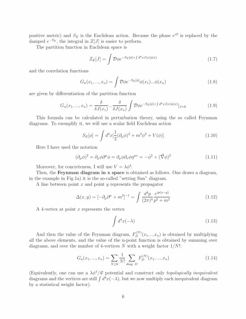
Moreover, for concreteness, I will use V = λφ4.Then, the Feynman diagram in x space is obtained as follows. One draws a diagram,

in the example in Fig.1a) it is the so-called ”setting Sun” diagram.A line between point x and point y represents the propagator

∆(x, y) = [−∂µ∂µ +m2]−1 =

∫

d4p

(2π)4

eip(x−y)

p2 +m2(1.12)

A 4-vertex at point x represents the vertex∫

d4x(−λ) (1.13)

And then the value of the Feynman diagram, F(N)D (x1, ...xn) is obtained by multiplying

all the above elements, and the value of the n-point function is obtained by summing overdiagrams, and over the number of 4-vertices N with a weight factor 1/N !:

Gn(x1, ..., xn) =∑

N≥0

1

N !

∑

diag D

F(N)D (x1, ..., xn) (1.14)

(Equivalently, one can use a λφ4/4! potential and construct only topologically inequivalentdiagrams and the vertices are still

∫

d4x(−λ), but we now multiply each inequivalent diagramby a statistical weight factor).

6

k1−p2−p3

x1 x2 x3 x4

a)

k1 p1

p2

p3

b)

d=2 d=4

d)

d=6

e)c)

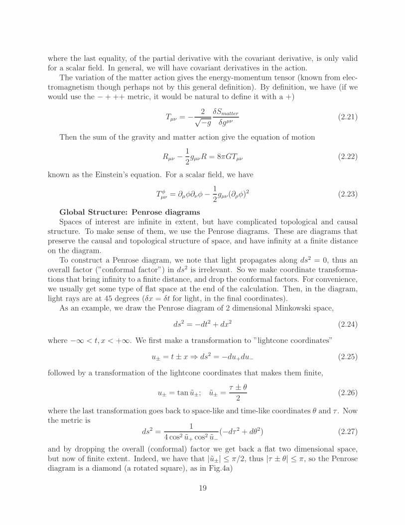
Figure 1: a) ”Setting sun” diagram in x-space. b) ”Setting sun” diagram in momentum space.c)anomalous diagram in 2 dimensions; d)anomalous diagram (triangle) in 4 dimensions;e)anomalous diagram (box) in 6 dimensions.

We mentioned that the VEV of the scalar field operator is an observable. In fact, thenormalized VEV in the presence of a source J(x),

φ(x; J) =J < 0|φ(x)|0 >J

J < 0|0 >J=

1

Z[J ]

∫

Dφe−S[φ]+J ·φφ(x) =δ

δJlnZ[J ] (1.15)

is called the classical field and satisfies an analog (quantum version) of the classical fieldequation.

S matricesFor real scattering, one constructs incoming and outgoing wavefunctions, representing

actual states, in terms of the idealized states of fixed (external) momenta ~k.Then one analyzes the scattering of these idealized states and at the end one convolutes

with the wavefunctions. The S matrix defines the transition amplitude between the idealizedstates by

< ~p1, ~p2, ...|S|~k1, ~k2, ... > (1.16)

The value of this S matrix transition amplitude is given in terms of Feynman diagrams inmomentum space. The diagrams are of a restricted type: connected (don’t contain dis-connected pieces) and amputated (which means that one does not use propagators for theexternal lines).

For instance, the setting sun diagram with external momenta k1 and p1 and internalmomenta p2, p3 and k1 − p2 − p3 in Fig.1b) is (in Euclidean space; for the S-matrix we mustgo to Minkowski space)

(2π)4δ4(k1 − p1)

∫

d4p2

(2π)4

d4p3

(2π)4λ2 1

p22 +m2

1

p23 +m2

1

(k1 − p2 − p3)2 +m24

(1.17)

7

The LSZ formulation relates S matrices in Minkowski space with correlation functionsas follows. The Fourier transformed n+m-point function near the physical poles k2

j = −m2

(for incoming particles) and p2i = −m2 (for outgoing particles) behaves as

Gn+m(p1, ..., pn; k1, ..., km) ∼(

n∏

i=1

√Zi

p2i +m2 + iǫ

)(

m∏

j+1

√Zi

k2j +m2 + iǫ

)

< p1, ..., pn|S|k1, .., km > (1.18)

where Z is the ”field renormalization” factor. For this reason, the study of correlationfunctions, which is easier, is preferred, since any physical process can be extracted fromthem as above.

If the external states are not states of a single field, but of a composite field O(x), e.g.

Oµν(x) = (∂µφ∂νφ)(x)(+...) (1.19)

it is useful to define Euclidean space correlation functions for these operators

< O(x1)...O(xn) >Eucl=

∫

Dφe−SEO(x1)...O(xn)

=δn

δJ(x1)...δJ(xn)

∫

Dφe−SE+R

d4xO(x)J(x)|J=0 (1.20)

which can be obtained from the generating functional

ZO[J ] =

∫

Dφe−SE+R

d4xO(x)J(x) (1.21)

Yang-Mills theory and gauge groupsElectromagnetismIn electromagnetism we have a gauge field

Aµ(x) = (φ(~x, t), ~A(~x, t)) (1.22)

with the field strength (containg the ~E and ~B fields)

Fµν = ∂µAν − ∂νAµ ≡ 2∂[µAν] (1.23)

The observables like ~E and ~B are defined in terms of Fµν and as such the theory has agauge symmetry under a U(1) group, that leaves Fµν invariant

δAµ = ∂µλ; δFµν = 2∂[µ∂ν]λ = 0 (1.24)

The Minkowski space action is

SMink = −1

4

∫

d4xF 2µν (1.25)

8

which becomes in Euclidean space (since A0 and x0 = t rotate in the same way)

SE =1

4

∫

d4x(Fµν)2 =

1

4

∫

d4xFµνFρσηµρηνσ (1.26)

The coupling of electromagnetism to a scalar field φ and a fermion field φ is obtained asfollows (note that in Minkowski space, we have ψ ≡ ψ+iγ0 and Lψ = −ψ(D/ + m)ψ, ∗ andhere ψ is independent of ψ and so there are no 1/2 factors, and φ∗ is independent of φ)

StotalE = SE,A +

∫

d4x[ψ(D/+m)ψ + (Dµφ)∗Dµφ]

D/ ≡ Dµγµ; Dµ ≡ ∂µ − ieAµ (1.27)

This is known as the minimal coupling. Then there is a U(1) local symmetry that extendsthe above gauge symmetry, namely

ψ′ = eieλ(x)ψ; φ′ = eieλ(x)φ (1.28)

under which Dµψ transforms as eieλDµψ, i.e transforms covariantly, as does Dµφ.The reverse is also possible, namely we can start with the action for φ and ψ only, with

∂µ instead of Dµ. It will have the symmetry in (1.28), except with a global parameter only.If we want to promote the global symmetry to a local one, we need to introduce a gaugefield and minimal coupling as above.

Yang-Mills fieldsYang-Mills fields Aaµ are self-interacting gauge fields, where a is an index belonging to a

nonabelian gauge group. There is thus a 3-point self-interaction of the gauge fields Aaµ, Abν , A

cρ,

that is defined by the constants fabc.The gauge group G has generators (T a)ij in the representation R. T a satisfy the Lie

algebra of the group,[Ta, Tb] = fab

cTc (1.29)

The group G is usually SU(N), SO(N). The adjoint representation is defined by (T a)bc =fabc. Then the gauge fields live in the adjoint representation and the field strength is

F aµν = ∂µA

aν − ∂νA

aµ + gfabcA

bµA

cν (1.30)

One can define A = AaTa and Fµν = F aµνTa in terms of which we have

Fµν = ∂µAν − ∂νAµ + g[Aµ, Aν ] (1.31)

(If one further defines the forms F = 1/2Fµνdxµ ∧ dxν and A = Aµdx

ν where wedge ∧denotes antisymmetrization, one has F = dA+ gA ∧ A).

The generators T a are taken to be antihermitian, their normalization being defined bytheir trace in the fundamental representation,

trT aT b = −1

2δab (1.32)

∗A note on conventions: If one instead uses the ηµν = (+ − −−) metric, then since γµ, γν = 2ηµν , wehave γµ = iγµ, so in Minkowski space one has ψ(iD/−m)ψ, with ψ = ψ+γ0

9

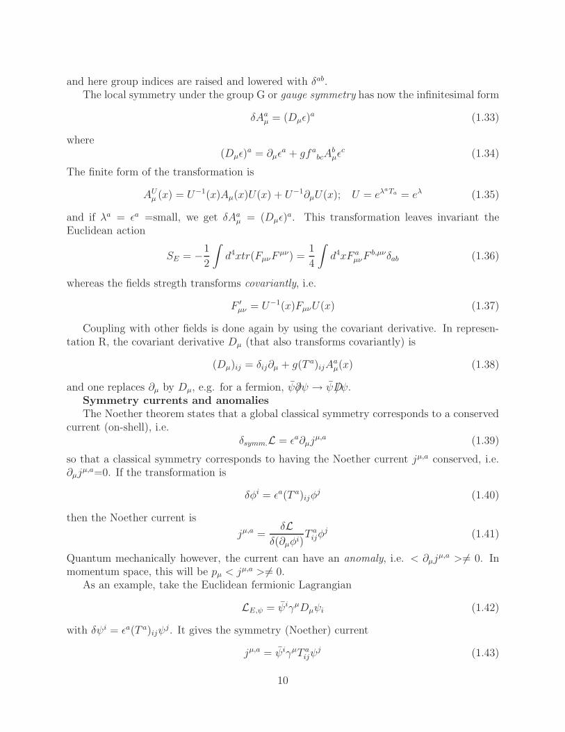
and here group indices are raised and lowered with δab.The local symmetry under the group G or gauge symmetry has now the infinitesimal form

δAaµ = (Dµǫ)a (1.33)

where(Dµǫ)

a = ∂µǫa + gfabcA

bµǫc (1.34)

The finite form of the transformation is

AUµ (x) = U−1(x)Aµ(x)U(x) + U−1∂µU(x); U = eλaTa = eλ (1.35)

and if λa = ǫa =small, we get δAaµ = (Dµǫ)a. This transformation leaves invariant the

Euclidean action

SE = −1

2

∫

d4xtr(FµνFµν) =

1

4

∫

d4xF aµνF

b,µνδab (1.36)

whereas the fields stregth transforms covariantly, i.e.

F ′µν = U−1(x)FµνU(x) (1.37)

Coupling with other fields is done again by using the covariant derivative. In represen-tation R, the covariant derivative Dµ (that also transforms covariantly) is

(Dµ)ij = δij∂µ + g(T a)ijAaµ(x) (1.38)

and one replaces ∂µ by Dµ, e.g. for a fermion, ψ∂/ψ → ψD/ψ.Symmetry currents and anomaliesThe Noether theorem states that a global classical symmetry corresponds to a conserved

current (on-shell), i.e.δsymm.L = ǫa∂µj

µ,a (1.39)

so that a classical symmetry corresponds to having the Noether current jµ,a conserved, i.e.∂µj

µ,a=0. If the transformation is

δφi = ǫa(T a)ijφj (1.40)

then the Noether current is

jµ,a =δL

δ(∂µφi)T aijφ

j (1.41)

Quantum mechanically however, the current can have an anomaly, i.e. < ∂µjµ,a > 6= 0. In

momentum space, this will be pµ < jµ,a > 6= 0.As an example, take the Euclidean fermionic Lagrangian

LE,ψ = ψiγµDµψi (1.42)

with δψi = ǫa(T a)ijψj . It gives the symmetry (Noether) current

jµ,a = ψiγµT aijψj (1.43)

10

Some observations can be made about this example. First, jaµ is a composite operator.Second, if ψi has also some gauge (local symmetry) indices (this is the reason why we wroteDµ instead of ∂µ), then jµ,a is gauge invariant, therefore it can represent a physical state.

One can use the formalism for composite operators and define the correlator

< jµ1,a1(x1)...jµn,an(xn) >=

δn

δAa1µ1(x1)...δAanνn

(xn)

∫

D[fields]e−SE+R

d4xjµ,a(x)Aaµ(x) (1.44)

which will then be a correlator of some external physical states (observables).We will see that this kind of correlators are obtained from AdS-CFT. The current anomaly

can manifest itself also in this correlator. jµ,a is inserted inside the quantum average, thusin momentum space, we could a priori have the anomaly

pµ1< jµ1,a1 ...jµn,an > 6= 0 (1.45)

In general, the anomaly is 1-loop only, and is given by polygon graphs, i.e. a 1-loop contribu-tion (a 1-loop Feynman diagram) to an n-point current correlator that looks like a n-polygonwith vertices = the x1, ..xn points. In d=2, only the 2-point correlator is anomalous by theFeynman diagram in Fig.1c, in d=4, the 3-point, by a triangle Feynman diagram, as inFig.1d, in d=6 the 4-point, by a box (square) graph, as in Fig.1e, etc.

Therefore, in d=4, the anomaly is called triangle anomaly.

Important concepts to remember

• Correlation functions are given by a Feynman diagram expansion and appear as deriva-tives of the partition function

• S matrices defining physical scatterings are obtained via the LSZ formalism from thepoles of the correlation functions

• Correlation functions of composite operators are obtained from a partition functionwith sources coupling to the operators

• Coupling of fields to electromagnetism is done via minimal coupling, replacing thederivatives d with the covariant derivatives D = d− ieA.

• Yang-Mills fields are self-coupled. Both the covariant derivative and the field strengthtransform covariantly.

• Classically, the Noether theorem associates every symmetry with a conserved current.

• Quantum mechanically, global symmetries can have an anomaly, i.e the current is notconserved, when inserted inside a quantum average.

• The anomaly comes only from 1-loop Feynman diagrams. In d=4, it comes from atriangle, thus only affects the 3-point function.

11

• In a gauge theory, the current of a global symmetry is gauge invariant, thus correspondsto some physical state.

References and further readingA good introductory course in quantum field theory is Peskin and Schroeder [1], and an

advanced level course that has more information, but is harder to digest, is Weinberg [2]. Inthis section I have only selected bits of QFT needed in the following.

12

Exercises, Section 1

1. If we have the partition function

ZE[J ] = exp−∫

d4x[(

∫

d4x0K(x, x0)J(x0))(−2x

2)(

∫

d4y0K(x, y0)J(y0))

+λ(

∫

d4x0K(x, x0)(J(x0)))3] (1.46)

write an expression for G2(x, y) and G3(x, y).

2. If we have the Euclidean action

SE =

∫

d4x[1

2(∂µφ)2 +

m2φ2

2+ λφ3] (1.47)

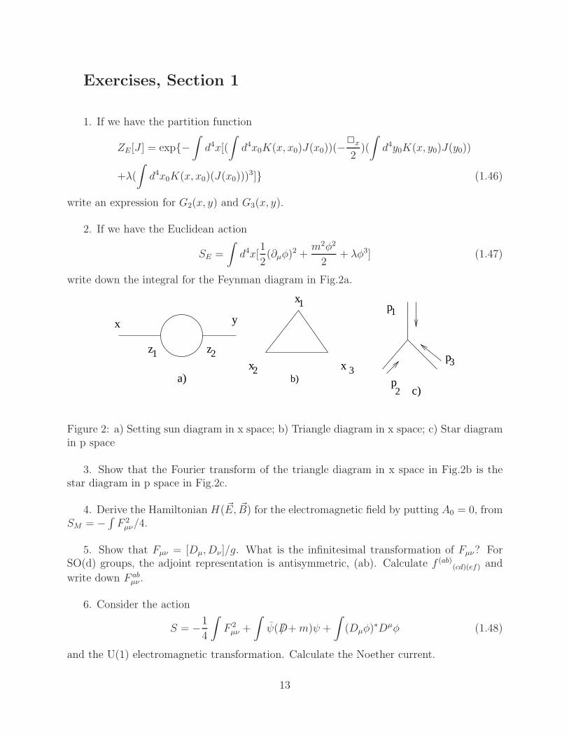
write down the integral for the Feynman diagram in Fig.2a.

c)

x y

z z1 2

a)

x

x x

1

2 3b)

p

p

p

1

2

3

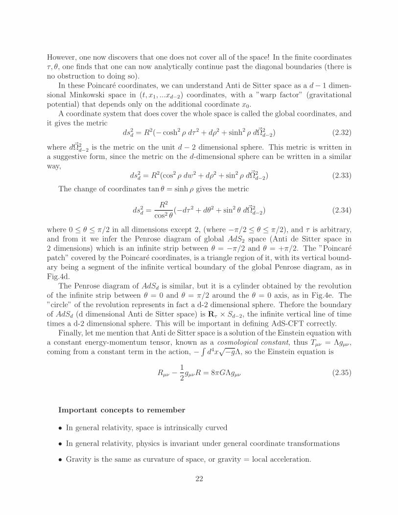
Figure 2: a) Setting sun diagram in x space; b) Triangle diagram in x space; c) Star diagramin p space

3. Show that the Fourier transform of the triangle diagram in x space in Fig.2b is thestar diagram in p space in Fig.2c.

4. Derive the Hamiltonian H( ~E, ~B) for the electromagnetic field by putting A0 = 0, fromSM = −

∫

F 2µν/4.

5. Show that Fµν = [Dµ, Dν ]/g. What is the infinitesimal transformation of Fµν? ForSO(d) groups, the adjoint representation is antisymmetric, (ab). Calculate f (ab)

(cd)(ef) and

write down F abµν .

6. Consider the action

S = −1

4

∫

F 2µν +

∫

ψ(D/+m)ψ +

∫

(Dµφ)∗Dµφ (1.48)

and the U(1) electromagnetic transformation. Calculate the Noether current.

13

2 Basics of general relativity; Anti de Sitter space.

Curved spacetime and geometryIn special relativity, one postulates that the speed of light is constant in all inertial

reference frames, i.e. c = 1. As a result, the line element

ds2 = −dt2 + d~x2 = ηijdxidxj (2.1)

is invariant, and is called the invariant distance. Here ηij = diag(−1, 1, ..., 1). Thereforethe symmetry group of general relativity is the group that leaves the above line elementinvariant, namely SO(1,3), or in general SO(1,d-1).

This Lorentz group is a generalized rotation group: The rotation group SO(3) is thegroup that leaves the 3 dimensional length d~x2 invariant. The Lorentz transformation is ageneralized rotation

x′i = Λijxj ; Λi

j ∈ SO(1, 3) (2.2)

Therefore the statement of special relativity is that physics is Lorentz invariant (invariantunder the Lorentz group SO(1,3) of generalized rotations).

In general relativity, one considers a more general spacetime, specifically a curvedspacetime, defined by the distance between two points, or line element,

ds2 = gij(x)dxidxj (2.3)

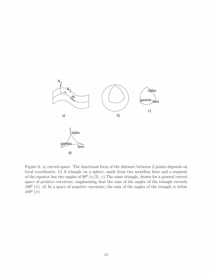
where gij(x) are arbitrary functions called the metric (sometimes one refers to ds2 as themetric). This situation is depicted in Fig.3a.

As we can see from the definition, the metric gij(x) is a symmetric matrix.To understand this, let us take the example of the sphere, specifically the familiar example

of a 2-sphere embedded in 3 dimensional space. Then the metric in the embedding space isthe usual Euclidean distance

ds2 = dx21 + dx2

2 + dx33 (2.4)

but if we are on a two-sphere we have the constraint

x21 + x2

2 + x23 = R2 ⇒ 2(x1dx1 + x2dx2 + x3dx3) = 0

⇒ dx3 = −x1dx1 + x2dx2

x3= − x1

√

R2 − x21 − x2

2

dx1 −x2

√

R2 − x21 − x2

2

dx2 (2.5)

which therefore gives the induced metric (line element) on the sphere

ds2 = dx21(1 +

x21

R2 − x21 − x2

2

) + dx22(1 +

x22

R2 − x21 − x2

2

) + 2dx1dx2x1x2

R2 − x21 − x2

2

= gijdxidxj

(2.6)So this is an example of a curved d-dimensional space which is obtained by embedding itinto a flat (Euclidean or Minkowski) d+1 dimensional space. But if the metric gij(x) arearbitrary functions, then one cannot in general embed such a space in flat d+1 dimensionalspace: there are d(d+1)/2 functions gij(x) to be obtained and only one function (in the above

14

d)

Xi

Xj

ds

a)

alpha

betagamma

b)c)

alpha

betagamma

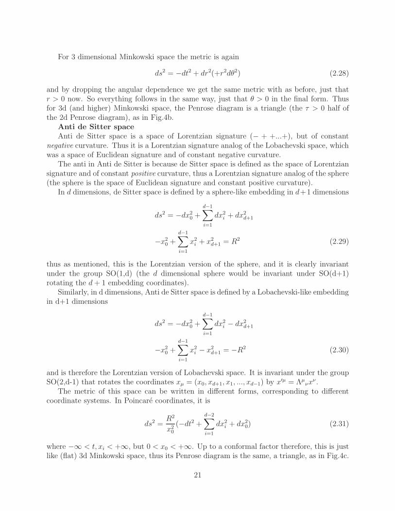
Figure 3: a) curved space. The functional form of the distance between 2 points depends onlocal coordinates. b) A triangle on a sphere, made from two meridian lines and a seqmentof the equator has two angles of 900 (π/2). c) The same triangle, drawn for a general curvedspace of positive curvature, emphasizing that the sum of the angles of the triangle exceeds1800 (π). d) In a space of negative curvature, the sum of the angles of the triangle is below1800 (π).

15

example, the function x3(x1, x2)), together with d coordinate transformations x′i = x′i(xj)available for the embedding. In fact, we will see that the problem is even more complicatedin general due to the signature of the metric (signs on the diagonal of the diagonalized matrixgij). Thus, even though a 2 dimensional metric has 3 components, equal to the 3 functionsavailable for a 3 dimensional embedding, to embed a metric of Euclidean signature in 3done needs to consider both 3d Euclidean and 3d Minkowski space, which means that 3dEuclidean space doesn’t contain all possible 2d surfaces.

That means that a general space can be intrinsically curved, defined not by embeddingin a flat space, but by the arbitrary functions gij(x) (the metric). In a general space, we

define the geodesic as the line of shortest distance∫ b

ads between two points a and b.

In a curved space, the triangle made by 3 geodesics has an unusual property: the sumof the angles of the triangle, α + β + γ is not equal to π. For example, if we make atriangle from geodesics on the sphere as in Fig.3b, we can easily convince ourselves thatα + β + γ > π. In fact, by taking a vertex on the North Pole and two vertices on theEquator, we get β = γ = π/2 and α > 0. This is the situation for a space with positivecurvature, R > 0: two parallel geodesics converge to a point (Fig.3c) (by definition, twoparallel lines are perpendicular to the same geodesic). In the example given, the two parallelgeodesics are the lines between the North Pole and the Equator: both lines are perpendicularto the equator, therefore are parallel by definition, yet they converge at the North Pole.

But one can have also a space with negative curvature, R < 0, for which α + β + γ < πand two parallel geodesics diverge, as in Fig.3d. Such a space is for instance the so-calledLobachevski space, which is a two dimensional space of Euclidean signature (like the twodimensional sphere), i.e. the diagonalized metric has positive numbers on the diagonal.However, this metric cannot be obtained as an embedding in a Euclidean 3d space, butrather an embedding in a Minkowski 3 dimensional space, by

ds2 = dx2 + dy2 − dz2; x2 + y2 − z2 = −R2 (2.7)

Einstein’s theory of general relativity makes two physical assumptions

• gravity is geometry: matter follows geodesics in a curved space, and the resultingmotion appears to us as the effect of gravity. AND

• matter sources gravity: matter curves space, i.e. the source of spacetime curvature(and thus of gravity) is a matter distribution.

We can translate these assumptions into two mathematically well defined physical prin-ciples and an equation for the dynamics of gravity (Einstein’s equation). The physicalprinciples are

• Physics is invariant under general coordinate transformations

x′i = x′i(xj) ⇒ ds2 = gij(x)dxidxj = g′ij(x

′)dx′idx′j (2.8)

16

• The Equivalence principle, which can be stated as ”there is no difference betweenacceleration and gravity” OR ”if you are in a free falling elevator you cannot distinguishit from being weightless (without gravity)”. This is only a local statement: for example,if you are falling towards a black hole, tidal forces will pull you apart before you reachit (gravity acts slightly differently at different points). The quantitative way to writethis principle is

mi = mg where ~F = mi~a (Newton′s law) and ~Fg = mg~g (gravitational force)(2.9)

In other words, both gravity and acceleration are manifestations of the curvature of space.Before describing the dynamics of gravity (Einstein’s equation), we must define the kine-

matics (objects used to describe gravity).As we saw, the metric gµν changes when we make a coordinate transformation, thus

different metrics can describe the same space. In fact, since the metric is symmetric, it hasd(d + 1)/2 components. But there are d coordinate transformations x′µ(xν) one can makethat leave the physics invariant, thus we have d(d − 1)/2 degrees of freedom that describethe curvature of space (different physics).

We need other objects besides the metric that can describe the space in a more invariantmanner. The basic such object is called the Riemann tensor, Rµ

νρσ. To define it, we firstdefine the inverse metric, gµν = (g−1)µν (matrix inverse), i.e. gµρg

ρσ = δσµ. Then we definean object that plays the role of ”gauge field of gravity”, the Christoffel symbol

Γµνρ =1

2gµσ(∂ρgνσ + ∂νgσρ − ∂σgνρ) (2.10)

Then the Riemann tensor is like the ”field strength of the gravity gauge field”, in that itsdefinition can be written as to mimic the definition of the field strength of an SO(n) gaugegroup (see exercise 5 in section 1),

F abµν = ∂µA

abν − ∂νA

abµ + Aacµ A

cbν −Aacν A

cbµ (2.11)

where a, b, c are fundamental SO(n) indices, i.e. ab (antisymmetric) is an adjoint index. Weput brackets in the definition of the Riemann tensor Rµ

νρσ to emphasize the similarity withthe above:

(Rµν)ρσ(Γ) = ∂ρ(Γ

µν)σ − ∂σ(Γ

µν)ρ + (Γµλ)ρ(Γ

λν)σ − (Γµλ)σ(Γ

λν)ρ (2.12)

the only difference being that here ”gauge” and ”spacetime” indices are the same.From the Riemann tensor we construct by contraction the Ricci tensor

Rµν = Rλµλν (2.13)

and the Ricci scalar R = Rµνgµν . The Ricci scalar is coordinate invariant, so it is truly an

invariant measure of the curvature of space. The Riemann and Ricci tensors are examplesof tensors. A contravariant tensor Aµ transforms as dxµ,

A′µ =∂x′µ

∂xνAν (2.14)

17

whereas a covariant tensor Bµ transforms as ∂/∂xµ, i.e.

B′µ =

∂xν

∂x′µBν (2.15)

and a general tensor transforms as the product of the transformations of the indices. Themetric gµν , the Riemann Rµ

νρσ and Ricci Rµν and R are tensors, but the Christoffel symbolΓµνρ is not (even though it carries the same kind of indices; but Γ can be made equal to zeroat any given point by a coordinate transformation).

To describe physics in curved space, we replace the Lorentz metric ηµν by the generalmetric gµν , and Lorentz tensors with general tensors. One important observation is that ∂µis not a tensor! The tensor that replaces it is the curved space covariant derivative, Dµ,modelled after the Yang-Mills covariant derivative, with (Γµν)ρ as a gauge field

DµTρν ≡ ∂µT

ρν + ΓρµσT

σν − ΓσµνT

ρσ (2.16)

We are now ready to describe the dynamics of gravity, in the form of Einstein’s equa-tion. It is obtained by postulating an action for gravity. The invariant volume of integra-tion over space is not ddx anymore as in Minkowski or Euclidean space, but ddx

√−g ≡ddx√

− det(gµν) (where the − sign comes from the Minkowski signature of the metric, whichmeans that det gµν < 0). The Lagrangian has to be invariant under general coordinatetransformations, thus it must be a scalar (tensor with no indices). There would be severalpossible choices for such a scalar, but the simplest possible one, the Ricci scalar, turns outto be correct (i.e. compatible with experiment). Thus, one postulates the Einstein-Hilbertaction for gravity †

Sgravity =1

16πG

∫

ddx√−gR (2.17)

The equations of motion of this action are

δSgravδgµν

= 0 : Rµν −1

2gµνR = 0 (2.18)

and as we mentioned, this action is not fixed by theory, it just happens to agree well withexperiments. In fact, in quantum gravity/string theory, Sg could have quantum correctionsof different functional form (e.g.,

∫

ddx√−gR2, etc.).

The next step is to put matter in curved space, since one of the physical principles wasthat matter sources gravity. This follows the above mentioned rules. For instance, the kineticterm for a scalar field in Minkowski space was

SM,φ = −1

2

∫

d4x(∂µφ)(∂νφ)ηµν (2.19)

and it becomes now

− 1

2

∫

d4x√−g(Dµφ)(Dνφ)gµν = −1

2

∫

d4x√−g(∂µφ)(∂νφ)gµν (2.20)

† Note on conventions: If we use the +−−− metric, we get a − in front of the action, since R = gµνRµν

and Rµν is invariant under constant rescalings of gµν .

18

where the last equality, of the partial derivative with the covariant derivative, is only validfor a scalar field. In general, we will have covariant derivatives in the action.

The variation of the matter action gives the energy-momentum tensor (known from elec-tromagnetism though perhaps not by this general definition). By definition, we have (if wewould use the − + ++ metric, it would be natural to define it with a +)

Tµν = − 2√−gδSmatterδgµν

(2.21)

Then the sum of the gravity and matter action give the equation of motion

Rµν −1

2gµνR = 8πGTµν (2.22)

known as the Einstein’s equation. For a scalar field, we have

T φµν = ∂µφ∂νφ− 1

2gµν(∂ρφ)2 (2.23)

Global Structure: Penrose diagramsSpaces of interest are infinite in extent, but have complicated topological and causal

structure. To make sense of them, we use the Penrose diagrams. These are diagrams thatpreserve the causal and topological structure of space, and have infinity at a finite distanceon the diagram.

To construct a Penrose diagram, we note that light propagates along ds2 = 0, thus anoverall factor (”conformal factor”) in ds2 is irrelevant. So we make coordinate transforma-tions that bring infinity to a finite distance, and drop the conformal factors. For convenience,we usually get some type of flat space at the end of the calculation. Then, in the diagram,light rays are at 45 degrees (δx = δt for light, in the final coordinates).

As an example, we draw the Penrose diagram of 2 dimensional Minkowski space,

ds2 = −dt2 + dx2 (2.24)

where −∞ < t, x < +∞. We first make a transformation to ”lightcone coordinates”

u± = t± x⇒ ds2 = −du+du− (2.25)

followed by a transformation of the lightcone coordinates that makes them finite,

u± = tan u±; u± =τ ± θ

2(2.26)

where the last transformation goes back to space-like and time-like coordinates θ and τ . Nowthe metric is

ds2 =1

4 cos2 u+ cos2 u−(−dτ 2 + dθ2) (2.27)

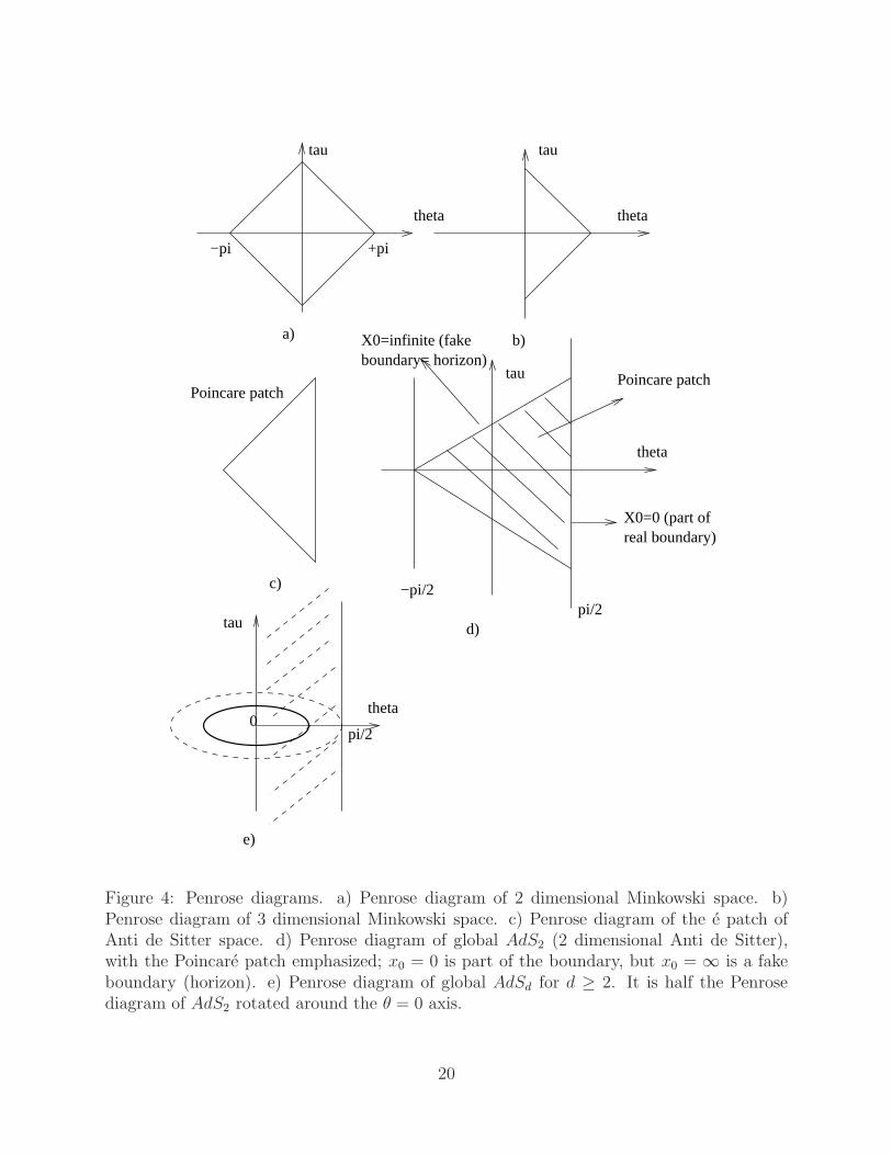
and by dropping the overall (conformal) factor we get back a flat two dimensional space,but now of finite extent. Indeed, we have that |u±| ≤ π/2, thus |τ ± θ| ≤ π, so the Penrosediagram is a diamond (a rotated square), as in Fig.4a)

19

e)

−pi +pi

theta

tau

a)

theta

tau

b)

c)

tau

theta

pi/2−pi/2

Poincare patchPoincare patch

X0=0 (part ofreal boundary)

X0=infinite (fakeboundary= horizon)

d)

theta

tau

pi/20

Figure 4: Penrose diagrams. a) Penrose diagram of 2 dimensional Minkowski space. b)Penrose diagram of 3 dimensional Minkowski space. c) Penrose diagram of the e patch ofAnti de Sitter space. d) Penrose diagram of global AdS2 (2 dimensional Anti de Sitter),with the Poincare patch emphasized; x0 = 0 is part of the boundary, but x0 = ∞ is a fakeboundary (horizon). e) Penrose diagram of global AdSd for d ≥ 2. It is half the Penrosediagram of AdS2 rotated around the θ = 0 axis.

20

For 3 dimensional Minkowski space the metric is again

ds2 = −dt2 + dr2(+r2dθ2) (2.28)

and by dropping the angular dependence we get the same metric with as before, just thatr > 0 now. So everything follows in the same way, just that θ > 0 in the final form. Thusfor 3d (and higher) Minkowski space, the Penrose diagram is a triangle (the τ > 0 half ofthe 2d Penrose diagram), as in Fig.4b.

Anti de Sitter spaceAnti de Sitter space is a space of Lorentzian signature (− + +...+), but of constant

negative curvature. Thus it is a Lorentzian signature analog of the Lobachevski space, whichwas a space of Euclidean signature and of constant negative curvature.

The anti in Anti de Sitter is because de Sitter space is defined as the space of Lorentziansignature and of constant positive curvature, thus a Lorentzian signature analog of the sphere(the sphere is the space of Euclidean signature and constant positive curvature).

In d dimensions, de Sitter space is defined by a sphere-like embedding in d+1 dimensions

ds2 = −dx20 +

d−1∑

i=1

dx2i + dx2

d+1

−x20 +

d−1∑

i=1

x2i + x2

d+1 = R2 (2.29)

thus as mentioned, this is the Lorentzian version of the sphere, and it is clearly invariantunder the group SO(1,d) (the d dimensional sphere would be invariant under SO(d+1)rotating the d+ 1 embedding coordinates).

Similarly, in d dimensions, Anti de Sitter space is defined by a Lobachevski-like embeddingin d+1 dimensions

ds2 = −dx20 +

d−1∑

i=1

dx2i − dx2

d+1

−x20 +

d−1∑

i=1

x2i − x2

d+1 = −R2 (2.30)

and is therefore the Lorentzian version of Lobachevski space. It is invariant under the groupSO(2,d-1) that rotates the coordinates xµ = (x0, xd+1, x1, ..., xd−1) by x′µ = Λµ

νxν .

The metric of this space can be written in different forms, corresponding to differentcoordinate systems. In Poincare coordinates, it is

ds2 =R2

x20

(−dt2 +

d−2∑

i=1

dx2i + dx2

0) (2.31)

where −∞ < t, xi < +∞, but 0 < x0 < +∞. Up to a conformal factor therefore, this is justlike (flat) 3d Minkowski space, thus its Penrose diagram is the same, a triangle, as in Fig.4c.

21

However, one now discovers that one does not cover all of the space! In the finite coordinatesτ, θ, one finds that one can now analytically continue past the diagonal boundaries (there isno obstruction to doing so).

In these Poincare coordinates, we can understand Anti de Sitter space as a d− 1 dimen-sional Minkowski space in (t, x1, ...xd−2) coordinates, with a ”warp factor” (gravitationalpotential) that depends only on the additional coordinate x0.

A coordinate system that does cover the whole space is called the global coordinates, andit gives the metric

ds2d = R2(− cosh2 ρ dτ 2 + dρ2 + sinh2 ρ d~Ω2

d−2) (2.32)

where d~Ω2d−2 is the metric on the unit d − 2 dimensional sphere. This metric is written in

a suggestive form, since the metric on the d-dimensional sphere can be written in a similarway,

ds2d = R2(cos2 ρ dw2 + dρ2 + sin2 ρ d~Ω2

d−2) (2.33)

The change of coordinates tan θ = sinh ρ gives the metric

ds2d =

R2

cos2 θ(−dτ 2 + dθ2 + sin2 θ d~Ω2

d−2) (2.34)

where 0 ≤ θ ≤ π/2 in all dimensions except 2, (where −π/2 ≤ θ ≤ π/2), and τ is arbitrary,and from it we infer the Penrose diagram of global AdS2 space (Anti de Sitter space in2 dimensions) which is an infinite strip between θ = −π/2 and θ = +π/2. The ”Poincarepatch” covered by the Poincare coordinates, is a triangle region of it, with its vertical bound-ary being a segment of the infinite vertical boundary of the global Penrose diagram, as inFig.4d.

The Penrose diagram of AdSd is similar, but it is a cylinder obtained by the revolutionof the infinite strip between θ = 0 and θ = π/2 around the θ = 0 axis, as in Fig.4e. The”circle” of the revolution represents in fact a d-2 dimensional sphere. Thefore the boundaryof AdSd (d dimensional Anti de Sitter space) is Rτ × Sd−2, the infinite vertical line of timetimes a d-2 dimensional sphere. This will be important in defining AdS-CFT correctly.

Finally, let me mention that Anti de Sitter space is a solution of the Einstein equation witha constant energy-momentum tensor, known as a cosmological constant, thus Tµν = Λgµν ,coming from a constant term in the action, −

∫

d4x√−gΛ, so the Einstein equation is

Rµν −1

2gµνR = 8πGΛgµν (2.35)

Important concepts to remember

• In general relativity, space is intrinsically curved

• In general relativity, physics is invariant under general coordinate transformations

• Gravity is the same as curvature of space, or gravity = local acceleration.

22

• The Christoffel symbol acts like a gauge field of gravity, giving the covariant derivative

• Its field strength is the Riemann tensor, whose scalar contraction, the Ricci scalar, isan invariant measure of curvature

• One postulates the action for gravity as (1/(16πG))∫ √−gR, giving Einstein’s equa-

tions

• To understand the causal and topological structure of curved spaces, we draw Penrosediagrams, which bring infinity to a finite distance in a controlled way.

• de Sitter space is the Lorentzian signature version of the sphere; Anti de Sitter spaceis the Lorentzian version of Lobachevski space, a space of negative curvature.

• Anti de Sitter space in d dimensions has SO(2, d− 1) invariance.

• The Poincare coordinates only cover part of Anti de Sitter space, despite having max-imum possible range (over the whole real line).

• Anti de Sitter space has a cosmological constant.

References and further readingFor a very basic (but not too explicit) introduction to general relativity you can try the

general relativity chapter in Peebles [3]. A good and comprehensive treatment is done in[4], which has a very good index, and detailed information, but one needs to be selectivein reading only the parts you are interested in. An advanced treatment, with an eleganceand concision that a theoretical physicist should appreciate, is found in the general relativitysection of Landau and Lifshitz [5], though it might not be the best introductory book. Amore advanced and thorough book for the theoretical physicist is Wald [6].

23

Exercises, section 2

1) Parallel the derivation in the text to find the metric on the 2-sphere in its usual form,

ds2 = R2(dθ2 + sin2 θdφ2) (2.36)

from the 3d Euclidean metric.

2) Show that on-shell, the graviton has degrees of freedom corresponding to a transverse(d-2 indices) symmetric traceless tensor.

3) Show that the metric gµν is covariantly constant (Dµgνρ = 0) by substituting theChristoffel symbols.

4) The Christoffel symbol Γµνρ is not a tensor, and can be put to zero at any point bya choice of coordinates (Riemann normal coordinates, for instance), but δΓµνρ is a tensor.Show that the variation of the Ricci scalar can be written as

δR = δρµgνσ(∂ρδΓ

µνσ − ∂σδΓ

µνρ) +Rνσδg

νσ (2.37)

5) Parallel the calculation in 2d to show that the Penrose diagram of 3d Minkwoski space,with an angle (0 ≤ φ ≤ 2π) supressed, is a triangle.

6) Substitute the coordinate transformation

X0 = R cosh ρ cos τ ; Xi = R sinh ρΩi; Xd+1 = R cosh ρ sin τ (2.38)

to find the global metric of AdS space from the embedding (2,d-1) signature flat space.

24

3 Basics of supersymmetry

In the 1960’s people were asking what kind of symmetries are possible in particle physics?We know the Poincare symmetry defined by the Lorentz generators Jab of the SO(1,3)

Lorentz group and the generators of 3+1 dimensional translation symmetries, Pa.We also know there are possible internal symmetries Tr of particle physics, such as the

local U(1) of electromagnetism, the local SU(3) of QCD or the global SU(2) of isospin. Thesegenerators will form a Lie algebra

[Tr, Ts] = frstTt (3.1)

So the question arose: can they be combined, i.e. [Ts, Pa] 6= 0, [Ts, Jab] 6= 0, such that maybewe could embed the SU(2) of isospin together with the SU(2) of spin into a larger group?

The answer turned out to be NO, in the form of the Coleman-Mandula theorem, whichsays that if the Poincare and internal symmetries were to combine, the S matrices for allprocesses would be zero.

But like all theorems, it was only as strong as its assumptions, and one of them was thatthe final algebra is a Lie algebra.

But people realized that one can generalize the notion of Lie algebra to a graded Liealgebra and thus evade the theorem. A graded Lie algebra is an algebra that has somegenerators Qi

α that satisfy not a commuting law, but an anticommuting law

Qiα, Q

jβ = other generators (3.2)

Then the generators Pa, Jab and Tr are called ”even generators” and the Qiα are called ”odd”

generators. The graded Lie algebra then is of the type

[even, even] = even; odd, odd = even; [even, odd] = odd (3.3)

So such a graded Lie algebra generalization of the Poincare + internal symmetries ispossible. But what kind of symmetry would a Qi

α generator describe?

[Qiα, Jab] = (...)Jcd (3.4)

means that Qiα must be in a representation of Jab (the Lorentz group). Because of the

anticommuting nature of Qiα (Qα, Qβ =others), we choose the spinor representation. But

a spinor field times a boson field gives a spinor field. Therefore when acting with Qiα (spinor)

on a boson field, we will get a spinor field.Therefore Qi

α gives a symmetry between bosons and fermions, called supersymmetry!

δ boson = fermion; δ fermion = boson (3.5)

Qα, Qβ is called the supersymmetry algebra, and the above graded Lie algebra is calledthe superalgebra.

Here Qiα is a spinor, with α a spinor index and i a label, thus the parameter of the

transformation law, ǫiα is a spinor also.

25

But what kind of spinor? In particle physics, Weyl spinors are used, that satisfy γ5ψ =±ψ, but in supersymmetry one uses Majorana spinors, that satisfy the reality condition

χC ≡ χTC = χ ≡ χ†iγ0 (3.6)

where C is the ”charge conjugation matrix”, that relates γm with γTm. In 4 Minkowskidimensions, it satisfies

CT = −C; CγmC−1 = −(γm)T (3.7)

And C is used to raise and lower indices, but since it is antisymmetric, one must define aconvention for contraction of indices (the order matters, i.e. χαψ

α = −χαψα).The reason we use Majorana spinors is convenience, since it is easier to prove various

supersymmetry identities, and then in the Lagrangian we can always go from a Majorana toa Weyl spinor and viceversa.

2 dimensional Wess Zumino modelWe will exemplify supersymmetry with the simplest possible models, which occur in 2

dimensions.A general (Dirac) fermion in d dimensions has 2[d/2] complex components, therefore in

2 dimensions it has 2 complex dimensions, and thus a Majorana fermion will have 2 realcomponents. An on-shell Majorana fermion (that satisfies the Dirac equation, or equationof motion) will then have a single component (since the Dirac equation is a matrix equationthat relates half of the components to the other half).

Since we have a symmetry between bosons and fermions, the number of degrees of freedomof the bosons must match the number of degrees of freedom of the fermions (the symmetrywill map a degree of freedom to another degree of freedom). This matching can be

• on-shell, in which case we have on-shell supersymmetry OR

• off-shell, in which case we have off-shell supersymmetry

Thus, in 2d, the simplest possible model has 1 Majorana fermion ψ (which has one degreeof freedom on-shell), and 1 real scalar φ (also one on-shell degree of freedom). We can thenobtain on-shell supersymmetry and get the Wess-Zumino model in 2 dimensions.

The action of a free boson and a free fermion in two Minkowski dimensions is ‡

S = −1

2

∫

d2x[(∂µφ)2 + ψ∂/ψ] (3.8)

and this is actually the action of the free Wess-Zumino model. From the action, the massdimension of the scalar is [φ] = 0, and of the fermion is [ψ] = 1/2 (the mass dimension of∫

d2x is −2 and of ∂µ is +1, and the action is dimensionless).To write down the supersymmetry transformation between the boson and the fermion,

we start by varying the boson into fermion times ǫ, i.e

δφ = ǫψ = ǫαψα = ǫβCβαψ

α (3.9)

‡Note that the Majorana reality condition implies that ψ = ψTC is not independent from ψ, thus wehave a 1/2 factor in the fermionic action

26

From this we infer that the mass dimension of ǫ is [ǫ] = −1/2. This also defines the orderof indices in contractions χψ (χψ = χαψ

α and χα = χβCβα). By dimensional reasons, forthe reverse transformation we must add an object of mass dimension 1 with no free vectorindices, and the only one such object available to us is ∂/, thus

δψ = ∂/φǫ (3.10)

We can check that the above free action is indeed invariant on-shell under this symmetry.For this, we must use the Majorana spinor identities, valid both in 2d and 4d

1) ǫχ = +χǫ; 2) ǫγµχ = −χγµǫ3) ǫγ5χ = +χγ5ǫ 4) ǫγµγ5χ = +χγµγ5ǫ; γ5 ≡ iγ0γ1γ2γ3 (3.11)

To prove, for instance, the first identity, we write ǫχ = ǫαCαβχβ , but Cαβ is antisymmetric

and ǫ and χ anticommute, being spinors, thus we get −χβCαβǫα = +χβCβαǫα. Then the

variation of the action gives

δS = −∫

d2x[−φ2δφ +1

2δψ∂/ψ +

1

2ψ∂/δψ] = −

∫

d2x[−φ2δφ + ψ∂/δψ] (3.12)

where in the second equality we have used partial integration together with identity 2) above.Then substituting the transformation law we get

δS = −∫

d2x[−φ2ǫψ + ψ∂/∂/φǫ] (3.13)

But we have

∂/∂/ = ∂µ∂νγµγν = ∂µ∂ν

1

2γµ, γν = ∂µ∂νg

µν = 2 (3.14)

and by using this identity, together with two partial integrations, we obtain that δS = 0.So the action is invariant without the need for the equations of motion, so it would seemthat this is an off-shell supersymmetry. However, the invariance of the action is not enough,since we have not proven that the above transformation law closes on the fields, i.e. that byacting twice on every field and forming the Lie algebra of the symmetry, we get back to thesame field, or that we have a representation of the Lie algebra on the fields. The graded Liealgebra of supersymmetry is generically of the type

Qiα, Q

jβ = 2(Cγµ)αβPµδ

ij + ... (3.15)

In the case of a single supersymmetry, for the 2d Wess-Zumino model we don’t have any+..., the above algebra is complete. In order to realize it on the fields, we need that (since Pµis represented by the translation ∂µ and Qα is represented by δǫα and we have a commutatorinstead of an anticommutator since φ→ δǫφ is a bosonic operation)

[δǫ1,α, δǫ2β

]

(

φψ

)

= 2ǫ2γµǫ1∂µ

(

φψ

)

(3.16)

27

We get that[δǫ1 , δǫ2]φ = 2ǫ2γ

ρǫ1∂ρφ (3.17)

as expected, but[δǫ1 , δǫ2]ψ = 2(ǫ2γ

ρǫ1)∂ρψ − (ǫ2γρǫ1)γρ∂/ψ (3.18)

thus we have an extra term that vanishes on-shell (i.e., if ∂/ψ = 0). So on-shell the algebrais satisfied and we have on-shell supersymmetry.

It is left as an exercise to prove these relations. One must use the previous spinor identitiestogether with new ones, called 2 dimensional ”Fierz identities” (or ”Fierz recoupling”),

Mχ(ψNφ) = −∑

j

1

2MOjNφ(ψOjχ) (3.19)

where M and N are arbitrary matrices, and the set of matrices Oj is = 1, γµ, γ5 (in2 Minkowski dimensions, γµ = (iτ1, τ2) and γ5 ≡ τ3, where τi are Dirac matrices). In4 Minkowski dimensions, the Fierz recoupling has 1/4 instead of 1/2 in front (since nowtr(OiOj) = 4δij instead of 2δij) and Oij = 1, γµ, γ5, iγµγ5, iγµν.

Off-shell supersymmetryIn 2 dimensions, an off-shell Majorana fermion has 2 degrees of freedom, but a scalar has

only one. Thus to close the algebra of the Wess-Zumino model off-shell, we need one extrascalar field F . But on-shell, we must get back the previous model, thus the extra scalar Fneeds to be auxiliary (non-dynamical, with no propagating degree of freedom). That meansthat its action is

∫

F 2/2, thus

S = −1

2

∫

d2x[(∂µφ)2 + ψ∂/ψ − F 2] (3.20)

From the action we see that F has mass dimension [F ] = 1, and the equation of motionof F is F = 0. The off-shell Wess-Zumino model algebra does not close on ψ, thus we needto add to δψ a term proportional to the equation of motion of F. By dimensional analysis,Fǫ has the right dimension. Since F itself is a (bosonic) equation of motion, its variation δFshould be the fermionic equation of motion, and by dimensional analysis ǫ∂/ψ is OK. Thusthe transformations laws are

δφ = ǫψ; δψ = ∂/φǫ+ Fǫ; δF = ǫ∂/ψ (3.21)

We can similarly check that these transformations leave the action invariant again, andmoreover now we have

[δǫ1, δǫ2]

φψF

= 2ǫ2γµǫ1∂µ

φψF

(3.22)

so the algebra closes off-shell, i.e. we have an off-shell representation of Qα, Qβ = 2(Cγµ)αβPµ.

4 dimensions

28

Similarly, in 4 dimensions the on-shell Wess-Zumino model has one Majorana fermion,which however now has 2 real on-shell degrees of freedom, thus needs 2 real scalars, A andB. The action is then

S0 = −1

2

∫

d4x[(∂µA)2 + (∂µB)2 + ψ∂/ψ] (3.23)

and the transformation laws are as in 2 dimensions, except nowB aquires an iγ5 to distinguishit from A, thus

δA = ǫψ; δB = ǫiγ5ψ; δψ = ∂/(A+ iγ5B)ǫ (3.24)

And again, off-shell the Majorana fermion has 4 degrees of freedom, so one needs to introduceone auxiliary scalar for each propagating scalar, and the action is

S = S0 +

∫

d4x[F 2

2+G2

2] (3.25)

with the transformation rules

δA = ǫψ; δB = ǫiγ5ψ; δψ = ∂/(A+ iγ5B)ǫ+ (F + iγ5G)ǫ

δF = ǫ∂/ψ; δG = ǫiγ5∂/ψ (3.26)

One can form a complex field φ = A+ iB and one complex auxiliary field M = F + iG, thusthe Wess-Zumino multiplet in 4 dimensions is (φ, ψ,M).

We have written the free Wess-Zumino model in 2d and 4d, but one can write downinteractions between them as well, that preserve the supersymmetry.

These were examples of N = 1 supersymmetry that is, there was only one supersymmetrygenerator Qα. The possible on-shell multiplets of N = 1 supersymmetry that have spins ≤ 1are

• The Wess-Zumino or chiral multiplet that we discussed, (φ, ψ).

• The vector multiplet (λA, AAµ ), where A is an adjoint index. The vector Aµ in 4dimensions has 2 on-shell degrees of freedom: it has 4 components, minus one gaugeinvariance symmetry parametrized by an arbitrary ǫa, δAAµ = ∂µǫ

A giving 3 off-shellcomponents. In the covariant gauge ∂µAµ = 0 the equation of motion k2 = 0 issupplemented with the constraint kµǫaµ(k) = 0 (ǫaµ(k) =polarization), which has only2 independent solutions. The two degrees of freedom of the gauge field match the 2degrees of freedom of the on-shell fermion.

For N ≥ 2 supersymmetry, we have Qiα with i = 1, ...,N . For N = 2, the possible

multiplets of spins ≤ 1 are

• The N = 2 vector multiplet, made of one N = 1 vector multiplet (Aµ, λ) and oneN = 1 chiral (Wess-Zumino) multiplet (ψ, φ).

• The N = 2 hypermultiplet, made of two N = 1 chiral multiplets (ψ1, φ1) and (ψ2, φ2).

29

For N = 4 supersymmetry, there is a single multiplet of spins ≤ 1, the N = 4 vectormultiplet, made of an N = 2 vector multiplet and a N = 2 hypermultiplet, or one N = 1vector multiplet (Aµ, ψ4) and 3 N = 1 chiral multiplets (ψi, φi), i = 1, 2, 3. They can berearranged into (Aaµ, ψ

ai, φ[ij]), where i = 1, .., 4 is an SU(4) = SO(6) index, [ij] is the6 dimensional antisymmetric representation of SU(4) or the fundamental representation ofSO(6), and i is the fundamental representation of SU(4) or the spinor representation ofSO(6). The field φ[ij] has complex entries but satisfies a reality condition,

φ†ij =

1

2φij ≡ ǫijklφkl (3.27)

The action of the N = 1 vector multiplet in 4d Minkowski space is (trTaTb = −δab/2)

SN=1SYM = −2

∫

d4xtr[−1

4F 2µν −

1

2ψD/ψ(+

D2

2)] (3.28)

where D/ = γµDµ, ψ = ψaTa is an adjoint fermion and D = DaTa is an auxiliary field for theoff-shell action. It is just the action of a gauge field, a spinor minimally coupled to it, andan auxiliary field. The transformation rules are

δAaµ = ǫγµψa

δψa = (−1

2γµνF a

µν + iγ5Da)ǫ

δDa = iǫγ5D/ψa (3.29)

They are similar to the rules of the Wess-Zumino multiplet, except for the gamma matrixfactors introduced in order to match the index structure, and for replacing ∂µφ with Fµν .

The action of the N = 4 Super Yang-Mills multiplet is §

SN=4SYM = −2

∫

d4x tr[−1

4F 2µν −

1

2ψiD/ψ

i − 1

2DµφijD

µφij

+igψi[φij, ψj] − g2[φij, φkl][φ

ij , φkl]] (3.30)

where Dµ = ∂µ + g[Aµ, ]. This action however has no (covariant and un-constrainedauxiliary fields) off-shell formulation.

The supersymmetry rules are

δAaµ = ǫiγµψai

δφ[ij]a =

i

2ǫ[iψj]a

δλai = −γµν

2F aµνǫ

i + 2iγµDµφa,[ij]ǫj − 2gfabc(φ

bφc)[ij]ǫj ; (φaφb)ij ≡ φa,ikφb,kj(3.31)

§This action and supersymmetry transformation rules can be obtained by ”dimensional reduction”, de-fined in the next section, of the N = 1 Super Yang-Mills action in 10 dimensions for the fields AM andΨΠ = Majorana -Weyl, Γ11Ψ = Ψ, Ψ = ΨTC10, with the reduction ansatz: ΓM = (γµ ⊗ 1, γ5 ⊗ γm),C10 = C4 ⊗ C6, AM = (Aµ, φm), φ[ij] ≡ φmγ

mij , γm

[ij] ≡ i/2(C6γmγ7)[ij], where the Clebsh-Gordan γm[ij] are

normalized, γm[ij]γ

[ij]n = δm

n . The Majorana conjugate in 4d is then defined as ψM ≡ ψTC4 ⊗C6 and the 10dWeyl condition restricts the spinors to be 4 dimensional, ΨΠ = ψαi, i = 1, .., 4

30

Important concepts to remember

• A graded Lie algebra can contain the Poincare algebra, internal algebra and supersym-metry.

• The supersymmetry Qα relates bosons and fermions.

• If the on-shell number of degrees of freedom of bosons and fermions match we have on-shell supersymmetry, if the off-shell number matches we have off-shell supersymmetry.

• For off-shell supersymmetry, the supersymmetry algebra must be realized on the fields.

• The prototype for all (linear) supersymmetry is the 2 dimensional Wess-Zumino model,with δφ = ǫψ, δψ = ∂/φǫ.

• The Wess-Zumino model in 4 dimensions has a fermion and a complex scalar on-shell.Off-shell there is also an auxiliary complex scalar.

• The on-shell vector multiplet has a gauge field and a fermion

• The N = 4 supersymmetric vector multiple (N = 4 SYM) has one gauge field, 4fermions and 6 scalars, all in the adjoint of the gauge field.

References and further readingFor a very basic introduction to supersymmetry, see the introductory parts of [7] and [8].

Good introductory books are West [9] and Wess and Bagger [10]. An advanced book that isharder to digest but contains a lot of useful information is [11]. An advanced student mightwant to try also volume 3 of Weinberg [2], which is also more recent than the above, but itis harder to read and mostly uses approaches seldom used in string theory. A book with amodern approach but emphasizing phenomenology is [12]. For a good treatment of spinorsin various dimensions, and spinor identities (symmetries and Fierz rearrangements) see [13].For an earlier but less detailed acount, see [14].

31

Exercises, section 3

1) Prove that the matrix

CAB =

(

ǫαβ 00 ǫαβ

)

; ǫαβ = ǫαβ =

(

0 1−1 0

)

(3.32)

is a representation of the 4d C matrix, i.e. CT = −C,CγµC−1 = −(γµ)T , if γµ is representedby

γµ =

(

0 σµ

σµ 0

)

; (σµ)αα = (1, ~σ)αα; (σµ)αα = (1,−~σ)αα (3.33)

2) Prove that if ǫ, χ are 4d Majorana spinors, we have

ǫγµγ5χ = +χγµγ5ǫ (3.34)

3) Prove that, for

S = −1

2

∫

d4x[(∂µφ)2 + ψ∂/ψ] (3.35)

we have

[δǫ1 , δǫ2]φ = 2ǫ2∂/ǫ1φ

[δǫ1 , δǫ2]ψ = 2(ǫ2γρǫ1)∂ρψ − (ǫ2γ

ρǫ1)γρ∂/ψ (3.36)

4) Show that the susy variation of the 4d Wess-Zumino model is zero, paralleling the 2dWZ model.

5) Check the invariance of the N=1 off-shell SYM action

S =

∫

d4x[−1

4(F a

µν)2 − 1

2ψaD/ψa +

1

2D2a] (3.37)

under the susy transformations

δAaµ = ǫγµψa; δψa = (−1

2σµνF a

µν + iγ5Da)ǫ; δDa = iǫγ5D/ψ

a (3.38)

6)Calculate the number of off-shell degrees of freedom of the on-shell N=4 SYM action.Propose a set of bosonic+fermionic auxiliary fields that could make the number of degreesof freedom match. Are they likely to give an off-shell formulation, and why?

32

4 Basics of supergravity

Vielbeins and spin connectionsWe saw that gravity is defined by the metric gµν , which in turn defines the Christoffel

symbols Γµνρ(g), which is like a gauge field of gravity, with the Riemann tensor Rµνρσ(Γ)

playing the role of its field strength.But there is a formulation that makes the gauge theory analogy more manifest, namely

in terms of the ”vielbein” eaµ and the ”spin connection” ωabµ . The word ”vielbein” comes fromthe german viel= many and bein=leg. It was introduced in 4 dimensions, where it is knownas ”vierbein”, since vier=four. In various dimensions one uses einbein, zweibein, dreibein,...(1,2,3= ein, zwei, drei), or generically vielbein, as we will do here.

Any curved space is locally flat, if we look at a scale much smaller than the scale of thecurvature. That means that locally, we have the Lorentz invariance of special relativity. Thevielbein is an object that makes that local Lorentz invariance manifest. It is a sort of squareroot of the metric, i.e.

gµν(x) = eaµ(x)ebν(x)ηab (4.1)

so in eaµ(x), µ is a ”curved” index, acted upon by a general coordinate transformation (sothat eaµ is a covariant vector of general coordinate transformations, like a gauge field), and ais a newly introduced ”flat” index, acted upon by a local Lorentz gauge invariance. That is,around each point we define a small flat neighbourhood (”tangent space”) and a is a tensorindex living in that local Minkowski space, acted upon by Lorentz transformations.

We can check that an infinitesimal general coordinate transformation (”Einstein” trans-formation) δxµ = ξµ acting on the metric gives

δξgµν(x) = (ξρ∂ρ)gµν + (∂µξρ)gρν + (∂νξ

ρ)gρν (4.2)

where the first term corresponds to a translation, but there are extra terms. Thus thegeneral coordinate transformations are the general relativity analog of Pµ translations inspecial relativity.

On the vielbein eaµ, the infinitesimal coordinate transformation gives

δξeaµ(x) = (ξρ∂ρ)e

aµ + (∂µξ

ρ)eaρ (4.3)

thus it acts only on the curved index µ. On the other hand, the local Lorentz transformation

δl.L.eaµ(x) = λab(x)e

bµ(x) (4.4)

is as usual.Thus the vielbein is like a sort of gauge field, with one covariant vector index and a gauge

group index. But there is one more ”gauge field” ωabµ , the ”spin connection”, which is definedas the ”connection” (≡ gauge field) for the action of the Lorentz group on spinors.

Namely, the curved space covariant derivative acting on spinors acts similarly to thegauge field covariant derivative on a spinor, by

Dµψ = ∂µψ +1

4ωabµ Γabψ (4.5)

33

This definition means that Dµψ is the object that transforms as a tensor under generalcoordinate transformations. It implies that ωabµ acts as a gauge field on any local Lorentzindex a.

If there are no dynamical fermions (i.e. fermions that have a kinetic term in the action)then ωabµ = ωabµ (e) is a fixed function, defined through the ”vielbein postulate”

T a[µν] = D[µeaν] = ∂[µe

aν] + ωab[µe

bν] = 0 (4.6)

Note that we can also start with

Dµeaν ≡ ∂µe

aν + ωabµ e

bν − Γρµνe

aρ = 0 (4.7)

and antisymmetrize, since Γρµν is symmetric. This is also sometimes called the vielbeinpostulate.

Here T a is called the ”torsion”, and as we can see it is a sort of field strength of eaµ, andthe vielbein postulate says that the torsion (field strength of vielbein) is zero.

But we can also construct an object that is a field strength of ωabµ ,

Rabµν(ω) = ∂µω

abν − ∂νω

abµ + ωabµ ω

bcν − ωacν ω

cbµ (4.8)

and this time the definition is exactly the definition of the field strength of a gauge field ofthe Lorentz group SO(1, d− 1) (see exercise 5, section 1; though there still are subtleties intrying to make the identification of ωabµ with a gauge field of the Lorentz group).

This curvature is in fact the analog of the Riemann tensor, i.e. we have

Rabρσ(ω(e)) = eaµe

−1,νbRµνρσ(Γ(e)) (4.9)

The Einstein-Hilbert action is then

SEH =1

16πG

∫

d4x(det e)Rabµν(ω(e))e−1,µ

a e−1,νb (4.10)

since√detg = det e.

The formulation just described of gravity in terms of e and ω is the second order formu-lation, so called because ω is not independent, but is a function of e.

But notice that if we make ω an independent variable in the above Einstein-Hilbertaction, the ω equation of motion gives exactly T aµν = 0, i.e. the vielbein postulate that weneeded to postulate before. Thus we might as well make ω independent without changing theclassical theory (only possibly the quantum version). This is then the first order formulationof gravity (Palatini formalism), in terms of independent (eaµ, ω

abµ ).

SupergravitySupergravity can be defined in two independent ways that give the same result. It is a

supersymmetric theory of gravity; and it is also a theory of local supersymmetry. Thus wecould either take Einstein gravity and supersymmetrize it, or we can take a supersymmetricmodel and make the supersymmetry local. In practice we use a combination of the two.

34

We want a theory of local supersymmetry, which means that we need to make the rigidǫα transformation local. We know from gauge theory that if we want to make a globalsymmetry local we need to introduce a gauge field for the symmetry. The gauge field wouldbe ”Aαµ” (since the supersymmetry acts on the index α), which we denote in fact by ψµα andcall the gravitino.

Here µ is a curved space index (”curved”) and α is a local Lorentz spinor index (”flat”).In flat space, an object ψµα would have the same kind of indices (”curved”=”flat”) and wecan then show that µα forms a spin 3/2 field, therefore the same is true in curved space.

The fact that we have a supersymmetric theory of gravity means that gravitino must betransformed by supersymmetry into some gravity variable, thus ψµα = Qα(gravity). Butthe index structure tells us that the gravity variable cannot be the metric, but somethingwith only one curved index, namely the vielbein.

Therefore we see that supergravity needs the vielbein-spin connection formulation ofgravity. To write down the supersymmetry transformations, we start with the vielbein. Inanalogy with the Wess-Zumino model where δφ = ǫφ or the vector multiplet where the gaugefield variation is δAaµ = ǫγµψ

a, it is easy to see that the vielbein variation has to be

δeaµ =k

2ǫγaψµ (4.11)

where k is the Newton constant and appears for dimensional reasons. Since ψ is like a gaugefield of local supersymmetry, we expect something like δAµ = Dµǫ. Therefore we must have

δψµ =1

kDµǫ; Dµǫ = ∂µǫ+

1

4ωabµ γabǫ (4.12)

plus maybe more terms.The action for a free spin 3/2 field in flat space is the Rarita-Schwinger action which is

SRS = − i

2

∫

d4xǫµνρσψµγ5γν∂ρψσ = −1

2

∫

ddxψµγµνρ∂νψρ (4.13)

where the first form is only valid in 4 dimensions and the second is valid in all dimensions(iǫµνρσγ5γν = γµρσ in 4 dimensions, γ5 = iγ0γ1γ2γ3). In curved space, this becomes

SRS = − i

2

∫

d4xǫµνρσψµγ5γνDρψσ = −1

2

∫

ddx(det e)ψµγµνρDνψρ (4.14)

N = 1 (on-shell) supergravity in 4 dimensionsWe are now ready to write down N = 1 on-shell supergravity in 4 dimensions. Its action

is just the sum of the Einstein-Hilbert action and the Rarita-Schwinger action

SN=1 = SEH(ω, e) + SRS(ψµ) (4.15)

and the supersymmetry transformations rules are just the ones defined previously,

δeaµ =k

2ǫγaψµ; δψµ =

1

kDµǫ (4.16)

However, this is not yet enough to specify the theory. We must specify the formalism andvarious quantities:

35

• second order formalism: The independent fields are eaµ, ψµ and ω is not an independentfield. But now there is a dynamical fermion (ψµ), so the torsion T aµν is not zero anymore,thus ω 6= ω(e)! In fact,

ωabµ = ωabµ (e, ψ) = ωabµ (e) + ψψ terms (4.17)

is found by varying the action with respect to ω, as in the ψ = 0 case:

δSN=1

δωabµ= 0 ⇒ ωabµ (e, ψ) (4.18)

• first order formalism: All fields, ψ, e, ω are independent. But now we must suplementthe action with a transformation law for ω. It is

δωabµ (first order) = −1

4ǫγ5γµψ

ab +1

8ǫγ5(γ

λψbλeaµ − γλψaλe

bµ)

ψab = ǫabcdψcd; ψab = e−1a

µe−1b

ν(Dµψν −Dνψµ) (4.19)

General features of supergravity theories4 dimensionsThe N = 1 supergravity multiplet is (eaµ, ψµα) as we saw, and has spins (2,3/2).It can also couple with other N = 1 supersymmetric multiplets of lower spin: the chiral

multiplet of spins (1/2,0) and the gauge multiplet of spins (1,1/2) that have been described,as well as the so called gravitino multiplet, composed of a gravitino and a vector, thus spins(3/2,1).

By adding appropriate numbers of such multiplets we obtain the N = 2, 3, 4, 8 supergrav-ity multiplets. Here N is the number of supersymmetries, and since it acts on the graviton,there should be exactly N gravitini in the multiplet, so that each supersymetry maps thegraviton to a different gravitino.

N = 8 supergravity is the maximal supersymmetric multiplet that has spins ≤ 2 (i.e.,an N > 8 multiplet will contains spins > 2, which are not very well defined), so we consideronly N ≤ 8.

Coupling to supergravity of a supersymmetric multiplet is a generalization of couplingto gravity, which means putting fields in curved space. Now we put fields in curved spaceand introduce also a few more couplings.

We will denote the N = 1 supersymmetry multiplets by brackets, e.g. (1,1/2), (1/2,0),etc. The supergravity multiplets are compose of the following fields:

N = 3 supergravity: Supergravity multiplet (2,3/2) + 2 gravitino multiplets (3/2,1) +one vector multiplet (1,1/2). The fields are then eaµ, ψiµ, Aiµ, λ, i=1,2,3.

N = 4 supergravity: Supergravity multiplet (2,3/2) + 3 gravitino multiplets (3/2,1) + 3vector multiplets (1,1/2) + one chiral multiplet (1/2,0). The fields are eaµ, ψiµ, Akµ, Bk

µ, λi, φ,

B, where i=1,2,3,4; k=1,2,3, A is a vector, B is an axial vector, φ is a scalar and B is apseudoscalar.

N = 8 supergravity: Supergravity multiplet (2,3/2) + 7 gravitino multiplets (3/2,1) + 21vector multiplets (1,1/2) + 35 chiral multiplets (1/2,0). The fields are eaµ, ψiµ, AIJµ , χijk, ν

36

which are: one graviton, 8 gravitinos ψiµ, 28 photons AIJµ , 56 spin 1/2 fermions χijk and 70scalars in the matrix ν.

In these models, the photons are not coupled to the fermions, i.e. the gauge couplingg = 0, thus they are ”ungauged” models. But these models have global symmetries, e.g. theN = 8 model has SO(8) global symmetry.

One can couple the gauge fields to the fermions, thus ”gauging” (making local) someglobal symmetry (e.g. SO(8)). Thus abelian fields become nonabelian (Yang-Mills), i.e.self-coupled. Another way to obtain the gauged models is by adding a cosmological constantand requiring invariance

δψiµ = Dµ(ω(e, ψ))ǫi + gγµǫi + gAµǫ

i (4.20)

where g is related to the cosmological constant, i.e. Λ ∝ g. Because of the cosmologicalconstant, it means that gauged supergravities have Anti de Sitter (AdS) backgrounds.

Higher dimensionsIn D > 4, it is possible to have also antisymmetric tensor fields Aµ1,...,µn, which are just

an extension of abelian vector fields, with field strength

Fµ1,...,µn+1= ∂[µ1

Aµ2,...,µn+1] (4.21)

and gauge invarianceδAµ1,...,µn = ∂[µ1

Λµ2,..,µn] (4.22)

and action∫

ddx(det e)F 2µ1,...,µn+1

(4.23)

The maximal model possible that makes sense as a 4 dimensional theory is the N = 1supergravity model in 11 dimensions, made up of a graviton eaµ, a gravitino ψµα and a 3index antisymmetric tensor Aµνρ.

But how do we make sense of a higher dimensional theory? The answer is the so calledKaluza-Klein (KK) dimensional reduction. The idea is that the extra dimensions(d− 4) are curled up in a small space, like a small sphere or a small d− 4-torus.

For this to happen, we consider a background solution of the theory that looks like, e.g.(in the simplest case) as a product space,

gΛΣ =

(

g(0)µν (x) 0

0 g(0)mn(y)

)

(4.24)

where g(0)µν (x) is the metric on our 4 dimensional space and g

(0)mn(y) is the metric on the extra

dimensional space.We then expand the fields of the higher dimensional theory around this background

solution in Fourier-like modes, called spherical harmonics. E.g., gµν(x, y) = g(0)µν (x) +

∑

n g(n)µν (x)Yn(y), with Yn(y) being the spherical harmonic (like eikx for Fourier modes).

37

Finally, dimensional reduction means dropping the higher modes, and keeping only thelowest Fourier mode, the constant one, e.g.

gΛΣ =

(

g(0)µν (x) + hµν(x) hµm(x)

hmν(x) g(0)mn(y) + hmn(x)

)

(4.25)

Important concepts to remember

• Vielbeins are defined by gµν(x) = eaµ(x)ebν(x)ηab, by introducing a Minkowski space in

the neighbourhood of a point x, giving local Lorentz invariance.

• The spin connection is the gauge field needed to define covariant derivatives acting onspinors. In the absence of dynamical fermions, it is determined as ω = ω(e) by thevielbein postulate: the torsion is zero.

• The field strength of this gauge field is related to the Riemann tensor.

• In the first order formulation (Palatini), the spin connection is independent, and isdetermined from its equation of motion.

• Supergravity is a supersymmetric theory of gravity and a theory of local supersymme-try.

• The gauge field of local supersymmetry and superpartner of the vielbein (graviton) isthe gravitino ψµ.

• Supergravity (local supersymmetry) is of the type δeaµ = (k/2)ǫγaψµ + ..., δψµ =(Dµǫ)/k + ...

• For each supersymmetry we have a gravitino. The maximal supersymmetry in d=4 isN = 8.

• Supergravity theories in higher dimensions can contain antisymmetric tensor fields.

• The maximal dimension for a supergravity theory is d=11, with a unique model com-posed of eaµ, ψµ, Aµνρ.

• A higher dimensional theory can be dimensionally reduced: expand in generalizedFourier modes (spherical harmonics) around a vacuum solution that contains a compactspace for the extra dimensions (like a sphere or torus), and keep only the lowest modes.

References and further readingAn introduction to supergravity, but not a very clear one is found in West [9] and Wess

and Bagger [10]. A good supergravity course, that starts at an introductory level and reachesquite far, is [14]. For the Kaluza-Klein approach to supergravity, see [15].

38

Exercises, section 4

1) Prove that the general coordinate transformation on gµν ,

g′µν(x′) = gρσ(x)

∂xρ

∂x′µ∂xσ

∂x′ν(4.26)

reduces for infinitesimal tranformations to

∂ξgµν(x) = (ξρ∂ρ)gµν + (∂µξρ)gρν + (∂νξ

ρ)gρµ (4.27)

2) Check that

ωabµ (e) =1

2eaν(∂µe

bν − ∂νe

bµ) −

1

2ebν(∂µe

aν − ∂νe

aµ) −

1

2eaρebσ(∂ρecσ − ∂σecρ)e

cµ (4.28)

satisfies the no-torsion (vielbein) constraint, T aµν = D[µeaν] = 0.

3) Check that the equation of motion for ωabµ in the first order formulation of gravity(Palatini formalism) gives T aµν = 0.

4) Write down the free gravitino equation of motion in curved space.

5) Find ωabµ (e, ψ) − ωabµ (e) in the second order formalism for N=1 supergravity.

6) Calculate the number of off-shell bosonic and fermionic degrees of freedom of N=8on-shell supergravity.

7) Consider the Kaluza Klein dimensional reduction ansatz from 5d to 4d

gΛΠ = φ−1/3

(

ηµν + hµν + φAµAν φAµφAν φ

)

(4.29)

Show that the action for the linearized perturbation hµν contains no factors of φ. (Hint: firstshow that for small hµν , where gµν = f(ηµν + hµν), Rµν(g) is independent of f).

39

5 Black holes and p-branes

The Schwarzschild solution (1916)The Schwarzschild solution is a solution to the Einstein’s equation without matter (Tµν =

0), namely

Rµν −1

2gµνR = 0 (5.1)

It is in fact the most general solution of Einstein’s equation with Tµν = 0 and spherical sym-metry (Birkhoff’s theorem, 1923). That means that by general coordinate transformationswe can always bring the metric to this form.

The 4 dimensional solution is

ds2 = −(1 − 2MG

r)dt2 +

dr2

1 − 2MGr

+R2dΩ22 (5.2)

It is remarkable that Schwarzschild derived this solution while fighting in World War I(literally, in the trenches: in fact, he even got ill there and died shortly after the end ofWWI).

The Newtonian approximation of general relativity is one of weak fields, i.e. gµν − ηµν ≡hµν ≪ 1 and nonrelativistic, i.e. v ≪ 1. In this limit, one can prove that the metric can bewritten in the general form

ds2 ≃ −(1 + 2U)dt2 + (1 − 2U)d~x2 = −(1 + 2U)dt2 + (1 − 2U)(dr2 + r2dΩ22) (5.3)

where U =Newtonian potential for gravity. In this way we recover Newton’s gravity theory.We can check that, with a O(ǫ) redefinition of r, the Newtonian approximation metricmatches the Schwarzschild metric if

U(r) = −2MG

r(5.4)

without any additional coordinate transformations, so at least its Newtonian limit is correct.Observation: Of course, this metric has a source at r = 0, which we can verify in the

Newtonian approximation: the solution is given by a point mass situated at r = 0. But thepoint is that if the space is empty at r ≥ r0, with r0 some arbitrary value, and is sphericallysymmetric, Birkhoff’s theorem says that we should obtain the Schwarzschild metric for r ≥ r0(and maybe a modified solution at r ≤ r0).

But the solution becomes apparently singular at rH = 2MG > 0, so it would seem thatit cannot reach its source at r = 0? This would be a paradoxical situation, since then whatwould be the role of the source? It would seem as if we don’t really need a point mass tocreate this metric.

If the Schwarzschild solution is valid all the way down to r = rH (not just to some r0 > rHwhich is the case for, let’s say, the gravitational field of the Earth, in which case r0 is theEarth’s radius), then we call that solution a Schwarzschild black hole.

So what does happen at rH = 2MG? We will try to understand it in the following.

40

First, let’s investigate the propagation of light (the fastest possible signal). If lightpropagates radially (dθ = dφ = 0), ds2 = 0 (light propagation) implies

dt =dr

1 − 2MGr

(5.5)

That means that near rH we have

dt ≃ 2MGdr

r − 2MG⇒ t ≃ 2MG ln(r − 2MG) → ∞ (5.6)

In other words, from the point of view of an asymptotic observer, that measures coor-dinates r, t (since at large r, ds2 ≃ −dt2 + dr2 + r2dΩ2

2), it takes an infinite time for lightto reach rH . And reversely, it takes an infinite time for a light signal from r = rH to reachthe observer at large r. That means that r = rH is cut-off from causal communication withr = rH . For this reason, r = rH is called an ”event horizon”. Nothing can reach, nor escapefrom the event horizon.

Observation: However, quantum mechanically, Hawking proved that black holes radiatethermally, thus thermal radiation does escape the event horizon of the black hole.

But is the event horizon of the black hole singular or not?The answer is actually NO. In gravity, the metric is not gauge invariant, it changes under

coordinate transformations. The appropriate gauge invariant (general coordinate transfor-mations invariant) quantity that measures the curvature of space is the Ricci scalar R. Onecan calculate it for the Schwarzschild solution and one obtains that at the event horizon

R ∼ 1

r2H

=1

(2MG)2= finite! (5.7)

Since the curvature of space at the horizon is finite, an observer falling into a black holedoesn’t feel anything special at r = rH , other than a finite curvature of space creating sometidal force pulling him apart (with finite strength).

So for an observer at large r, the event horizon looks singular, but for an observerfalling into the black hole it doesn’t seem remarkable at all. This shows that in generalrelativity, more than in special relativity, different observers see apparently different events:For instance, in special relativity, synchronicity of two events is relative which is still true ingeneral relativity, but now there are more examples of relativity.

An observer at fixed r close to the horizon sees an apparently singular behaviour: Ifdr = 0, dΩ = 0, then

ds2 = − dt2

1 − 2MGr

= −dτ 2 ⇒ dτ =√−g00dt =

dt√

1 − 2MGr

(5.8)

thus the time measured by that observer becomes infinite as r → rH , and we get an infinitetime dilation: an observer fixed at the horizon is ”frozen in time” from the point of view ofthe observer at infinity.

41

Since there is no singularity at the event horizon, it means that there must exist coordi-nates that continue inside the horizon, and there are indeed. The first such coordinates werefound by Eddington (around 1924!) and Finkelstein (in 1958! He rediscovered it, whithoutbeing aware of Eddington’s work, which shows that the subject of black holes was not sopopular back then...). The Eddington-Finkelstein coordinates however don’t cover all thegeometry.

The first set of coordinates that cover all the geometry was found by Kruskal and Szekeresin 1960, and they give maximum insight into the physics, so we will describe them here.

One first introduces the ”tortoise” coordinates r∗ by imposing

dr

1 − 2MGr

= dr∗ ⇒ r∗ = r + 2MG ln(r

2MG− 1) (5.9)

which gives the metric

ds2 = (1 − 2MG

r)(−dt2 + dr2

∗) + r2(r∗)dΩ22 (5.10)

Next one introduces null (lightcone) coordinates

u = t− r∗; v = t+ r∗ (5.11)

such that light (ds2 = 0) travels at u=constant or v=constant. Finally, one introducesKruskal coordinates,

u = −4MGe−u

4MG ; v = +4MGev

4MG (5.12)

Then the region r ≥ 2MG becomes −∞ < r∗ < +∞, thus −∞ < u ≤ 0, 0 ≤ v < +∞. Butthe metric in Kruskal coordinates is

ds2 = −2MG

re−

r2MGdudv + r2dΩ2

2 (5.13)

where r stands for the implicit r(u, v). This metric is non-singular at the horizon r = 2MG,thus can be analytically continued for general values of u, v, covering all the real line, having4 quadrants instead of one!

The resulting Kruskal diagram (diagram in Kruskal coordinate) in given in Fig.5a andthe Penrose diagram (which can be obtained from (5.13) as a subset of the flat 2 dimensionalspace ds2 = dudv Penrose diagram) is given in Fig.5b. The Penrose diagram of a physicalblack hole, obtained from a collapsing star, is given in Fig.5c.

Solutions with chargeThe Reissner-Nordstrom black hole is obtained by adding a charge Q at r = 0, giving

the solution

ds2 = −(1 − 2MG

r+Q2G

r2)dt2 +

dr2

1 − 2MGr

+ Q2Gr2

+ r2dΩ22 (5.14)

together with the electric field given by

Frt =Q

r2⇒ At = −Q

r(5.15)

42

horizon

r=0 singularity

r=0 singularity

III

II

IV

Ifuture eventhorizon

past event horizon

III

I

IV

II

b)

r=0 singularity

r=0

i0(spatialinfinity)

i+(temporal infinity)

null infinity

null past infinity

c)

a)

Figure 5: a) Kruskal diagram of the Schwarzschild black hole. b) Penrose diagram of theeternal Schwarzschild black hole (time independent solution). The dotted line gives thecompletion to the Penrose diagram of flat 2 dimensional (Minkowski) space. c) Penrosediagram of a physical black hole, obtained from a collapsing star (the curved line). The dottedline gives the completion to the Penrose diagram of flat d > 2 dimensional (Minkowski) space.

43

that is, the electric field of a point charge. The event horizon is now where 1 − 2MG/r +Q2G/r2 = 0. In the following we will put G = 1 for simplicity, and G can be reintroducedby dimensional analysis. The event horizon is at

r = r± = M ±√

M2 −Q2 (5.16)

thus we have now 2 horizons, instead of one, and the metric can be rewritten as

ds2 = −∆dt2 +dr2

∆+ r2dΩ2

2; ∆ = (1 − r+r

)(1 − r−r

) (5.17)

However, if M < Q, there is no horizon at all, just a ”naked singularity” at r = 0(the singularity is not covered by a horizon), which is believed to be excluded on physicsgrounds: there are a number of theorems saying that naked singularities should not occurunder certain very reasonable assumptions. Therefore we must have M ≥ Q.

The case M = Q is special and is called the ”extremal black hole”. Its metric is

ds2 = −(1 − M

r)2dt2 +

(

dr

1 − Mr

)2

+ r2dΩ22 (5.18)

and by a change of coordinates r = M + r we get

ds2 = − 1

(1 + Mr

)2dt2 + (1 +

M

r)2(dr2 + r2dΩ2

2) (5.19)

Here

H = 1 +M

r(5.20)

is a harmonic function, i.e. it satisfies

∆(3)H ∝ Mδ3(r) (5.21)

So we see that the extremal solutions are defined by a harmonic function in 3 dimensions.One can put this Reissner-Nordstrom black hole inside an Anti de Sitter space as well as

follows. The Anti de Sitter metric can be written (by a coordinate transformation) as

ds2 = −(1 − Λr2

3)dt2 +

dr2

1 − Λr2

3

+ r2dΩ22 (5.22)

Then the Anti de Sitter charged black hole metric is

ds2 = −∆dt2 +dr2

∆+ r2dΩ2

2; ∆ ≡ 1 − 2M

r+Q

r2− Λr2

3(5.23)

The only other parameter one can add to a black hole is the angular momentum J , inwhich case however the metric is quite complicated. There are so called ”no hair theorems”

44

stating that black holes are characterized only by Q,M and J (any other charge or parameterwould be called ”hair” of the black hole).

P-branesBlack holes that extend in p spatial dimensions are called p-branes (the terminology

comes from the word mem-brane which is now called a 2-brane, that is, extends in 2 spatialdimensions). We will especially be interested in ”extremal p-branes” (M = Q).

In 4 dimensions, the only localized extremal p-branes are the black holes. An extendedobject can be either a cosmic string (one spatial extension) or a domain wall (two spatialextensions). However, we will shortly see that the extremal p-branes are defined by harmonicfunctions in D-p-1 dimensions (the black hole, with p=0, in d=4 is defined by a harmonicfunction in 3 dimensions). Thus for a cosmic string, the harmonic function would be in 2dimensions, which is H = ln |z| (z = x1 + ix2), whereas for a domain wall, the harmonicfunction would be in one dimension, which is H = 1 + a|x|. In both cases, the harmonicfunction increases away from its source, so both the cosmic string and the domain wallextremal p-brane solutions would affect the whole space. They are therefore quite unlikeblack holes, and not quite physical.

But in dimensions higher than 4, we can have black-hole like objects extended in pspatial dimensions that are localized in space (don’t grow at infinity). These are the ”blackp-branes”, and have complicated metrics.

We will focus on the case of D=10, which is the case relevant for string theory, as wewill see in the next section. We will also focus on extremal objects (with Q = M), whichare very special: in fact, they are very relevant for string theory. The solution of the D=10supergravity theory that approximates string theory at moderate energies is of the generaltype

ds2string = H−1/2

p (−dt2 + d~x2p) +H1/2

p (dr2 + r2dΩ28−p)

= H−1/2p (−dt2 + d~x2

p) +H1/2p d~x2

9−p)

e−2φ = Hp−3

2p

A01...p = −1

2(H−1

p − 1) (5.24)

where Hp is a harmonic function of ~x9−p, i.e.

∆(9−p)Hp ∝ Qδ(9−p)(xi); ⇒ Hp = 1 +(...)Q

r7−p(5.25)

Here ds2string is known as the ”string metric” and is related to the usual ”Einstein metric”

defined until now byds2

Einstein = e−φ/2ds2string (5.26)

and A01...p is some antisymmetric tensor (”gauge”) field present in the 10 dimensional super-gravity theory (there are several), and φ is the ”dilaton” field, which is a scalar field that isrelated to the string theory coupling constant by gs = e−φ.

We noted that a black hole carries electric (or magnetic!) charge Q, with respect to theelectromagnetic potential Aµ. Specifically, for a static electric charge, only A0 is nonzero.

45

That means that there is a source coupling in the action, of the type∫

d4xjµAµ =

∫

j0A0 (5.27)

and if j0 is taken to be the current of a static charge, j0 = Qδ3(x), the source term givesrise by the Aµ equation of motion to the solution of nonzero A0.

Similarly, we find that a p-brane carries electric charge Q with respect to the p+1-formfield Aµ1...µp+1

. By analogy with the above means that there should be a source coupling∫

ddxjµ1...µp+1Aµ1...µp+1→∫

j01...pA01...p (5.28)

It therefore follows that a source for the A01...p field will be of the type j01...p = Qδ(d−p−1)(x),which is therefore an object extended in p spatial dimensions plus time. The solution of thesource coupling is an object with nonzero A01..p, and indeed the p-brane has such a nonzerofield.

Important concepts to remember

• The Schwarzschild solution is the most general solution with spherical symmetry andno sources. Its source is localed behind the event horizon.

• If the solution is valid down to the horizon, it is called a black hole.

• Light takes an infinite time to reach the horizon, from the point of view of the far awayobserver, and one has an infinite time dilation at the horizon (”frozen in time”).

• Classically, nothing escapes the horizon. (quantum mechanically, Hawking radiation)

• The horizon is not singular, and one can analytically continue inside it via the Kruskalcoordinates.

• Black hole solutions with charge have Q ≥ M . The Q = M solutions (extremal) aredefined by a harmonic function and have a collapsed horizon.

• P-brane solutions are (extremal) black hole solutions that extend in p spatial dimen-sions. They also carry charge under an antisymmetric tensor field Aµ1...µp+1

, and aredetermined by a harmonic function.

References and further readingFor an introduction to black holes, the relevant chapters in [4] are probably the best. A

very advanced treatment of the topological properties of black holes can be found in Hawkingand Ellis [16]. They also have a good treament of Penrose diagrams, so one can read thatselectively. For an introduction to p-brane solutions of supergravity, see the review [17]. Tounderstand the usefulness of p-branes, one can look at Tseytlin’s ”harmonic function rule”developped in [18]. To understand the meaning of extremal p-branes, one can look at therule for making an extremal solution non-extremal, found in [19].

46

Exercises, section 5

1) Check the transformation from Schwarzschild coordinates to Kruskal coordinates.

2) Find the equation for the r=0 singularity in Kruskal coordinates (the singularitycurve on the Kruskal diagram). Hint: calculate the equation at r = r0=arbitrary and thenextrapolate the final result to r = 0.

3) Check that the transformation of coordinates r/R = sinh ρ takes the AdS metricbetween the global coordinates

ds2 = R2(−dt2 cosh2 ρ+ dρ2 + sinh2 ρdΩ2) (5.29)

and the coordinates (here R =√

−Λ/3)

ds2 = −(1 − Λ

3r2)dt2 +

dr2

1 − Λ3r2

+ r2dΩ2 (5.30)

4) Check that H = 1 + a/r7−p is a good harmonic function for a p-brane. Check thatr=0 is an event horizon (it traps light).

5) The electric current of a point charge is jµ = Qdxµ

dτδd−1(xµ(τ)). Write an expression

for the p+1-form current of a p-brane, jµ1...µp+1.

47

6 String theory actions and spectra

The Nambu-Goto actionString theory is the theory of relativistic strings. That is, not strings like the violin

strings, but strings that move at the speed of light. They don’t have a compression mode(the energy density along a string is not a Lorentz invariant, so cannot appear as a physicalvariable in a relativistic theory). They only have a vibration mode, unlike, e.g. a massivecosmic string or a violin string.

However, they can have tension, which resists against pulling the string apart (energyper unit length). The point is that if one stretches the string the energy density stays thesame, just the length increases, thus energy = tension × length.

Because they have tension, the only possible action for a string is the one that minimizesthe area traversed by the string, i.e. the ”worldsheet”. The coordinates for the position ofthe string are Xµ(σ, τ), where σ =worldsheet length and τ = worldsheet time, i.e. (σ, τ) areintrinsic coordinates on the surface drawn by the moving string (worldsheet), as in Fig.6a.The string action, due to Nambu and Goto, is

SNG = − 1

2πα′

∫

dτdσ√

det(hab) (6.1)

where 1/(2πα′) = T is the string tension. The metric hab is the metric induced on theworldsheet by the motion through spacetime, or ”pull-back” of the spacetime metric,

hab(σ, τ) = ∂aXµ∂bX

νgµν(X) (6.2)

and dτdσ√

det h is the ”volume element” (infinitesimal area) on the worldsheet. This issimilar to the case of the metric on a 2-sphere in 3 dimensional Euclidean space given as anexample at the begining of the General Relativity section. As there, the metric is obtainedby the fact that the metric on the worldsheet is expressed in two ways

ds2|on M = dξadξbhab(ξ) = gµν(X)dXµdXν ; ξa = (σ, τ) (6.3)

What does the Nambu-Goto action calculate though? It calculates Xµ(σ, τ), the stringtrajectory through spacetime.

So, an analog of the string action is the particle action in flat space

S = −m∫

ds = −m∫

dτ

√

−XµXνηµν = −m∫

dt√

1 − ~v2 (6.4)

By varying it with respect to Xµ we get the equation of motion

−md

dτ[Xνηµν

√

−(Xµ)2

] = −m d

dτ[Xνηµν ] = 0 ⇒ d2

dτXµ = 0 (6.5)

Here X = dX/dτ and we have used −(Xµ)2 = −ds2/dτ 2 ≡ 1.

48

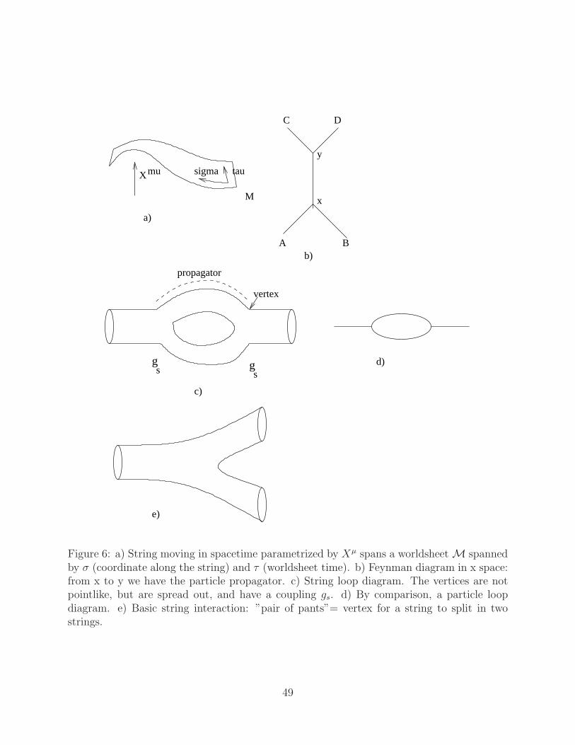
e)

tausigma

M

Xmu

a)

x

y

A B

C D

b)

g gss

propagator

vertex

c)

d)

Figure 6: a) String moving in spacetime parametrized by Xµ spans a worldsheet M spannedby σ (coordinate along the string) and τ (worldsheet time). b) Feynman diagram in x space:from x to y we have the particle propagator. c) String loop diagram. The vertices are notpointlike, but are spread out, and have a coupling gs. d) By comparison, a particle loopdiagram. e) Basic string interaction: ”pair of pants”= vertex for a string to split in twostrings.

49

This of course looks a little trivial, we obtain just the free motion in a straight line.However, if the write the same action in curved space instead, replacing ηµν → gµν , we willget the free motion along a geodesic in spacetime. The geodesic equation is then nontrivial,and can be understood as the interaction of the particle with the gravitational field. In moregeneral terms, we can say that background fields (like the metric) appearing in the particleor string actions will give interaction effects.

But what is the usefulness of the particle action for quantum field theory?Let us suppose that we don’t know how to do quantum field theory and/or the precise

theory we have. We can then still construct Feynman diagrams, considered as describingactual particles propagating in spacetime, for instance as in Fig.6b.

To construct such a Feynman diagram, we need

• the propagator from x to y

• the vertex factor at x and y: this contains the coupling g, thus it defines a particulartheory.

• rules about how to integrate (in this case,∫

d4x∫

d4y). For particles, this is obvious,but for strings, we need to carefully define a path integral construction. There aresubtleties due to the possibility of overcounting if we use naive integration.

The propagator from x to y for a massless particle is (here, 2= kinetic operator)

< x|2−1|y >=

∫ ∞

0

dτ < y|e−τ2|x > (6.6)

But now we can use a trick: A massive nonrelativistic particle has the Hamiltonian H =~p2/(2m) = 2/(2m) (if ~p and 2 live in an Euclidean x space). Using m = 1/2 we get H = 2

and therefore we can use quantum mechanics to write a path integral representation of thetransition amplitude

< y|e−τH|x >=

∫ y

x

Dx(t)e− 1

4

R τ0dtx2

(6.7)

Since H = 2, we use this representation to express the propagator of a massless relativisticparticle in (6.6) as

< x|2−1|y >=

∫ τ

0

∫ y

x

Dx(t)e− 1

4Sp (6.8)

where Sp =∫ τ

0dtx2 is the massless particle action (in fact, we have not quite seen that yet,

we just looked at the massive particle action, but we will see on the next page that it is aswe said).

So the particle action defines the propagator, and to complete the perturbative definitionof the quantum field theory by Feynman diagrams we need to add the vertex rules (specifyingthe interactions of the theory: for instance, in the V = λφ4 example in section 1 we had avertex −λ), as well as the integration rules (trivial, in the case of the particle).

We will do the same for string theory: we will define perturbative string theory by definingFeynman diagrams. We will write a worldsheet action that will give the propagator, andthen interaction rules and integration rules.

50

Before that however, we need to understand better the possible particle actions.Specifically, we can write down a first order action for the massive particle that is morefundamental than the one we wrote. First order means that we introduce an independent”worldline metric” field, γττ (τ), not defined by embedding in the spacetime metric. Rather,we will use the vielbein, or rather einbein in this case, e(τ) =

√

−γττ (τ).Then we can write the first order particle action (

√det γ × γττ = e−1(τ))

Sp =1

2

∫

dτ(e−1(τ)dXµ

dτ

dXν

dτηµν − em2) (6.9)

Then the e(τ) equation of motion gives

− 1

e2X2 −m2 = 0 ⇒ e2(τ) = −X

µXµ

m2(6.10)

Substituting in Sp we get

Sp =1

2

∫

dτ

[

m√

−X2X2 −

√

−X2

mm2

]

= −m∫

dτ

√

−XµXµ = Sp (6.11)

so we do indeed get the previous (second order) action by solving the e(τ) equation of motionand substituting.

Note that now we can take the m→ 0 limit of the first order action Sp, unlike the secondorder action Sp which is proportional to m. The first order action has a gauge invariance,which is the reparametrization invariance, τ → τ ′(τ) that gives e → edτ/dτ ′. Therefore bya reparametrization τ ′(τ) I can set e to whatever value. In particular it is convenient tochoose the gauge e = 1. Then the massless particle action in this gauge is

Sm=0,e=1 =

∫

dτdXµ

dτ

dXν

dτηµν (6.12)

which is the result we used above, in the calculation of the massless particle propagator.Note that now the equation of motion for Xµ(τ) is

d

dτ(dXµ

dτ) = 0 (6.13)

Note also that, since we work in the gauge e = 1, we must impose the e(τ) equation ofmotion as a constraint on the solutions. It gives

− ds2

dτ 2=dXµ

dτ

dXν

dτηµν = 0 (6.14)

which is just the statement that the particle is massless.We now go back to strings and mimic what we did for particles, to write down a first

order action. It is called the Polyakov action. In flat spacetime (gµν = ηµν), it is

SP [X, γ] = − 1

4πα′

∫

dσdτ√−γγab∂aXµ∂bX

νηµν (6.15)

51

Here γab is an independent metric on the worldsheet. Its equation of motion gives

hab −1

2γab(γ

cdhcd) = 0 (6.16)

wherehab = ∂aX

µ∂bXνηµν (6.17)

as before. We then obtain

hab√−h

=γab√−γ ⇒ SP = − 1

2πα′

∫

dτdσ√−h = SNG (6.18)

thus indeed, the Polyakov action is the first order form of the Nambu-Goto action.The Polyakov action has the following invariances:

• Spacetime Poincare invariance

• Worldsheet diffeomorphism invariance, defined by two transformations (σ′(σ, τ), τ ′(σ,τ)), that give X ′µ(σ′, τ ′) = Xµ(σ, τ)

• Worldsheet Weyl invariance: for any ω(σ, τ), we have

X ′µ(σ, τ) = Xµ(σ, τ); γ′ab(σ, τ) = e2ω(σ,τ)γab(σ, τ) (6.19)

The Weyl invariance is very important in the following, and is not present in the Nambu-Goto action. Therefore the Polyakov form is more fundamental. Classically, the two actionsare equivalent, as we saw. But quantum mechanically, they are not.

Strings have spatial extension, but that means we also need boundary conditions forthem. They can be open, in which case the endpoints of the string are different (and canhave either Neumann or Dirichlet boundary conditions) or closed. We will study closedstrings in the following.

Closed string spectrum.The Polyakov action has 3 worldsheet invariances (defined by arbitrary functions): 2

diffeomorphisms (σ′(σ, τ) and τ ′(σ, τ)) and one Weyl invariance (ω(σ, τ)). That means thatwe can choose the 3 independent elements of the symmetric matrix hαβ(σ, τ) (the worldsheetmetric) to be anything we want. We will choose the gauge

hαβ = ηαβ =

(

−1 00 1

)

(6.20)

called the conformal gauge. Then, the Polyakov action in flat spacetime becomes

S = −T2

∫

d2σηαβ∂αXµ∂βX

νηµν (6.21)

The Xµ equation of motion gives the 2 dimensional wave equation

2Xµ =

(

∂2

∂σ2− ∂2

∂τ 2

)

Xµ = −4∂+∂−Xµ = 0 (6.22)

52

We define

σ± = τ ± σ; ∂± =1

2(∂τ ± ∂σ) (6.23)

Then the general solution of the 2 dimensional wave equation is

Xµ(σ, τ) = XµR(σ−) +Xµ

L(σ+) (6.24)

For a closed string, that is everything, since we don’t need to impose a boundary condi-tion, and we can expand this general solution in Fourier modes:

XµR =

1

2xµ +

l2

2pµ(τ − σ) +

il

2

∑

n 6=0

1

nαµne

−2in(τ−σ)

XµL =

1

2xµ +

l2

2pµ(τ + σ) +

il

2

∑

n 6=0

1

nαµne

−2in(τ+σ) (6.25)

Note that the zero mode has been written in a particular way: The zero mode is Xµ =xµ + l2pµτ , where l2/2 = α, but has been split into a Xµ

L part and a XµR part.

As in the case of the particle action, because we work in a gauge for 2 dimensionalinvariance, we need to impose the equation of motion of the worldsheet metric γab as aconstraint

2√γ

δS

δγαβ≡ Tαβ = 0 (6.26)

So the constraint is that the worldsheet energy-momentum tensor must be equal to zero.We expand also this constraint in Fourier modes and define

Lm =T

2

∫ π

0

e−2imσT−−dσ

Lm =T

2

∫ π

0

e2imσT++dσ (6.27)

The zero modes of the constraints give

L0 + L0 = 0 ⇒ pµpµ ≡M2 =2

α′

∑

n≥1

(αµ−nαµn + αµ−nα

µn) (6.28)

We are still left with L0 − L0 = 0 and Ln = 0, Ln = 0 (n 6= 0) to impose.But there is in fact a quantum correction, that one can calculate, giving in fact L0 + L0 =

2, and modifying the mass relation (see below). One quantizes these oscillation modes (asis familiar from, let’s say, the phonon quantization or the quantization of sounds modes ina cavity) by setting, for m > 0 (There are several ways of quantizing, but we can think ofkeeping just the µ = 1, ..., D − 2, transverse components. When quantizing, one must alsoimpose the physical state conditions Lm| >= 0, Lm| >= 0.)

αµm =√maµm; αµ−m =

√ma†m

µ; [aµm, a

†n

ν] = δmnδ

µν (6.29)

53

Then one obtains the closed string mass spectrum

α′M2 = −4 + 2∑

m,µ

m(Nµm + Nµ

m); Nµm = a†m

µaµm = number operator (6.30)

where the constant actually depends on dimension. Quantum consistency requires D=26,and then the constant is −4 as above.

So this string theory makes sense at the quantum level only if it is defined in 26 di-mensions, so in order to get a 4 dimensional theory we must use the Kaluza-Klein idea ofdimensional reduction.

There is now an extra condition for physical states. It can be understood in two ways.We can say that is the invariance of translations along the closed string, σ → σ + s, whichmeans that Pσ, the translation generator along σ, should act trivially on states, and it turnsout that we must impose

Pσ = −2π

l

∑

m,µ

m(Nµm − Nµ

m) = 0 (6.31)

Another way of saying this is that Pσ is proportional to L0 − L0, which was still left to beimposed on states. In any case, that means that

N ≡∑

m,µ

mNµm =

∑

m,µ

mNµm ≡ N (6.32)

Then, the closed string spectrum starts with a tachyon of α′M2 = −4. It is denotedby |0, 0; k >, that is, vacuum for αm oscillators, vacuum for αm oscillators, and with zero-mode momentum p = k. At the next level, we have 1 excitation on the level m = 1. Butthen Nµ

m = Nµm = 1 and we must have both a α−1 and a α−1 excitation. We get that this

excitation has α′M2 = −4 + 2 · 2 = 0, so these are massless states. These states will be ofthe type

αµ−1αν−1|0, 0; k > (6.33)

This will then be a tensor state Aµν (with two spacetime indices). It decomposes into asymmetric traceless tensor part gµν , an antisymmetric tensor part Bµν and a trace partφ. These massless modes of the string correspond to the graviton gµν , a field called theantisymmetric tensor field (or B field) Bµν and the dilaton field φ.

This was for the simplest string action, the bosonic string, and we saw that the groundstate is tachyonic, thus unstable (M2 < 0 means that we are perturbing a potential V (Φ),where Φ is the tachyon field, around a maximum, V (Φ) ≃ V0 +M2(δΦ)2; M2 < 0 insteadof a minimum). It then means that this vacuum will decay to the true vacuum. The bosonicstring thus is not very well undestood.

Instead, one defines the superstring, which is a supersymmetric string. One extends thePolyakov action to a supersymmetric action. Then the spectrum of the supersymmetricclosed string is in part obtained by projecting out some of the bosonic string states. Thetachyon ground state is projected out, but the massless states remain.

So the superstring has a ground state composed of the massless states (gµν , Bµν , φ),together with some supersymmetric partners. Quantum consistency of the superstring now

54

requires D=10. Thus we still need to use the Kaluza-Klein idea of dimensional reduction inorder to get to a 4 dimensional theory.

Above this ground state, the string modes have increasing mass. Each string modecorresponds to a spacetime field of a given mass. But since the mass scale of the modes isset by 1/α′, in the limit of α′ → 0 only the massless fields remain. The massless fields thenaquire VEVs that correspond to classical backgrounds (with quantum corrections).

By self-consistency, we write down the propagation of the string in backgrounds generatedby the massless string modes, i.e. gµν , Bµν , φ. The action is

S = − 1

4πα′

∫

d2σ[√hhαβ∂αX

µ∂βXνgµν(X

ρ) + ǫαβ∂αXµ∂βX

νBµν(Xρ) − α′

√hR(2)Φ(Xρ)]

(6.34)where R(2) is the 2 dimensional Ricci scalar and the quantity

1

4π

∫

d2σ√hR(2) = χ (6.35)

is a topological invariant, i.e. a negative integer that counts the number of holes the topologyof the 2 dimensional surface has (times −2, specifically, χ = 2(1−g)). But e−S contains thene−χΦ = (eΦ)2(g−1). Therefore, the addition of a hole to a whorldsheet, which is interpretedas an extra loop in the quantum interaction of a string, as in Fig.6c, gives a factor of e2Φ,prompting the identification of eΦ with the string coupling constant, gs.

This procedure, of putting the string in a background (”condensate”) of its own groundstate modes, needs a self-consistency condition: the procedure must preserve the originalinvariances of the action, specifically Weyl invariance (or conformal invariance, see nextsection). Imposing Weyl invariance of the action in fact turns out to give the equations ofmotion for gµν , Bµν , φ.

When using this self-consistency on the full superstring, the background will be a su-persymmetric theory of gravity = supergravity! It will contain the fields gµν , Bµν , φ amongothers. That means that the α′ → 0 (low energy limit) of string theory, which is the theoryof the massless backgrounds of string theory, will be supergravity in 10 dimensions.

There are different types of string theories in 10 dimensions, and correspondingly differenttypes of supergravities (type IIA, massless and massive, type I and type IIB). In this course,we will be focusing on type IIB string theory and type IIB supergravity. The type refersto how many 10 dimensional supersymmetries, or minimal fermions (Majorana-Weyl, i.e.satsfying both the Majorana condition and the chiral -Weyl- condition) there are in thetheory. Type I refers to a single fermion, with 16 components (half the maximal 32). TypeIIA refers to two fermions of opposite chiralities, and type IIB to two fermions of the samechirality.

Now, to construct string theory perturbatively, as for the particle case, we constructS matrices through Feynman diagrams, as in Fig.6c. The basic interaction that gives theFeynman digrams is the ”pants diagram” in Fig.6e. The Polyakov action will define thepropagator, the vertices are defined such that we reproduce supergravity vertices in the lowenergy limit α′ → 0, and as noted, one needs to define integration carefully at each looporder, since as we can see the vertex is ”smoothed out”.

55

Important concepts to remember

• String theory is the theory of relativistic strings, with tension = energy/ length.

• The string action is the area spanned by the moving string, and its minimization isdue to its tension

• For the Feynman diagram construction of quantum field theory, we need the particleaction to define the propagator, the vertex factors to define the theory, and integrationrules.

• The first order particle action is more fundamental: it contains the massless case. ThePolyakov string action is also more fundamental: it has more symmetries.

• By fixing a gauge, the closed string action reduces to free 2 dimensional bosons, whichcontain left and right moving wave modes.

• By quantizing these modes, we get the particle spectrum. The massless particles arethe graviton, an antisymmetric tensor and a scalar.

• The bosonic string is unstable. The superstring is stable and lives in 10 dimensions,thus we need to use Kaluza-Klein dimensional reduction.

• Self-consistent backgrounds for the string are given by the theory of the massless modesof the superstring, namely supergravity.

• Thus the low energy limit (α′ → 0) of string theory is supergravity.

• We will be working with IIB supergravity, which has two minimal 10d fermions of thesame chirality.

• One knows how to construct string theory S matrices from Feynman diagrams bydefining the propagator, vertices and integration rules.

References and further readingPerhaps the best introduction to string theory (tailored to MIT undergraduates) is

Zwiebach [20]. A good advanced book, though somewhat dated by now (it doesn’t haveany of the developments relating to the ”second superstring revolution” dealing with D-branes and dualities) is Green, Schwarz and Witten [21]. It still contains the most in depthexplanations of many classic string theory problems. A modern book that also contains bothD-branes and dualities is Polchinski [22], from one of the people who started the second su-persting revolution. The most up to date book, containing many of the research problemsbeing developed now (but as a result with less in depth coverage of the basics of stringtheory), is [23]. Finally, a book focused more on D-branes is [24].

56

Exercises, section 6

1) Write down the worldline reparametrization invariance for the particle, both the finiteand infinitesimal versions.

2) Calculate Lm, Lm and L0 + L0.

3) Derive Pσ.

4) Write down the states of the first massive closed string level.

5) Show that the coupling to Bµν is of the type of p-brane sources, thus a string is a1-brane source for the field Bµν .

57

7 Elements of conformal field theory; D-branes

Conformal transformations and the conformal groupConsider flat space (either Euclidean or Minkowski), and quantum field theory in it.

Conformal transformations are then generalizations of the scale transformations

x′µ = αxµ ⇒ ds2 = d~x′2 = α2d~x2 (7.1)

Before we define conformal transformations, let’s understand scale transformations infield theory.

The procedure of renormalization involves a cut-off ǫ and bare coupling λ0 and massm0. For example, dimensional regularization of scalar field theory for V (φ) = m2φ2/2 + λφ4

gives

λ0 = µǫ(λ+

∞∑

k=1

ak(λ)

ǫk); m2

0 = m2(1 +

∞∑

k=1

bk(λ)

ǫk) (7.2)

where µ is the renormalization scale, out of which we extract the renormalized couplingλ = λ(µ, ǫ;λ0, m0), which in general depends on scale.

This running of the coupling constant with the scale is characterized by the β function,

β(λ, ǫ) = µdλ

dµ|m0,λ0,ǫ (7.3)

A scale invariant theory (i.e. a theory independent of α in (7.1)) must then be µ-independent, thus have a zero β function. There are two ways in which this can happen:

• β = 0 everywhere, which means a cancellation of Feynman diagrams that implies thereare no infinities. OR

• a nontrivial interacting theory: the β function is nontrivial, but has a zero (fixed point)away from λ = 0, at which a nontrivial (nonperturbative) theory emerges: a conformalfield theory. For the case in Fig.7c, ΛF is called an IR stable point. Indeed, if λ > λF ,β(λ) > 0, thus λ decreases if µ decreases (thus in the IR). And f λ < λF , β(λ) < 0,thus λ increases if µ again decreases (in the IR). That means that if we go to the IR,wherever we start, we are driven to λ = λF , that has β(λF ) = 0.

If we have a theory with classical scale invariance, it must be respected in the quantumtheory. But a priori there could be a quantum anomaly (that is, there are Feynman diagramsthat could potentially break scale invariance of the quantum averaged theory). So one mustrequire as a consistency of the theory the absence of quantum anomalies to Weyl (scale)invariance, which will give constraints on the theory.

Most theories that are quantum mechanically scale invariant (thus have β = 0), have alarger invariance, called conformal invariance.

In flat d dimensions, i.e. on R1,d−1, conformal transformations are defined by xµ → x′µ(x)such that

dx′µdx′µ = [Ω(x)]−2dxµdxµ (7.4)

58

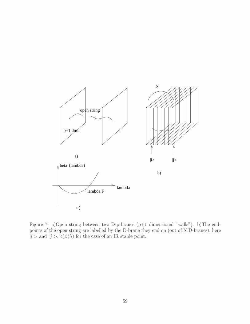
c)

p+1 dim.

open string

a)

N

|i> |j>

b)

lambda

beta

lambda F

(lambda)

Figure 7: a)Open string between two D-p-branes (p+1 dimensional ”walls”). b)The end-points of the open string are labelled by the D-brane they end on (out of N D-branes), here|i > and |j >. c)β(λ) for the case of an IR stable point.

59

Note that conformal invariance is NOT the same as general coordinate invariance (thoughconformal transformations obviously are a subclass of general coordinate transformations),since the metric is modified, from flat ds2 = dx′µdx

′µ to ”conformally flat” ds2 = [Ω(x)]−2

dxµdxµ, yet we are studying flat space field theories. This is a statement of the fact thatconformal transformations are generalizations of scale transformations (7.1) that change thedistance between points.

The infinitesimal conformal transformation is then

x′µ = xµ + vµ(x); Ω(x) = 1 − σv(x)

⇒ ∂µvν + ∂νvµ = 2σvδµν ⇒ σv =1

d∂ · v (7.5)

D=2 is special, and will be analyzed separately. But except for d=2, the most generalsolution to this equation is

vµ(x) = aµ + ωµνxν + λxµ + bµx2 − 2xmub · x (7.6)

with ωµν = −ωνµ (antisymmetric) and σv(x) = λ − 2b · x. Thus the parameters of confor-mal transformations are λ, aµ, bµ, ωµν , corresponding respectively to scale transformations,translations, a new type of transformations, and rotations. The new type of transforma-tions parametrized by bµ is called ”special conformal transformations”. Together there are1 + d + d + d(d − 1)/2 = (d + 1)(d + 2)/2 components for the parameters of conformaltransformatios.

These transformations form together a symmetry group. Its generators are: Pµ for aµand Jµν for ωµν forming together the Poincare group, as expected. For them, we havethe particular case of Ω(x) = 1. The new generators are Kµ for the special conformaltransformations bµ and dilatation generator D for λ. Counting shows that we can assemblethese generators in a group defined by an antisymmetric (d+ 2) × (d+ 2) matrix,

JMN =

Jµν Jµ,d+1 Jµ,d+2

−Jν,d+1 0 D−Jν,d+2 −D 0

(7.7)

where

Jµ,d+1 =Kµ − Pµ

2; Jµ,d+2 =

Kµ + Pµ2

; Jd+1,d+2 = D (7.8)

By looking at the Lie algebra of JMN we find that the metric in the d + 2 direction isnegative, thus the symmetry group is SO(2, d). So conformal invariance in flat (1, d − 1)dimensions (d > 2) corresponds to the symmetry group SO(2, d), the same as the symmetrygroup of d+ 1-dimensional Anti de Sitter space, AdSd+1.

This is in fact the first hint of a relation between d-dimensional conformal field theory,i.e. a field theory on d-dimensional Minkwoski space that is invariant under the conformalgroup, and a gravity theory in d+1 dimensional Anti de Sitter space. The precise relationbetween the two will be AdS-CFT, defined in the next section.

60

A comment is in order here. Strictly speaking, SO(2,d) is a group that only containselements continously connected to the identity, however the conformal group is an extensionthat also contains the inversion

I : x′µ =xµx2

⇒ Ω(x) = x2 (7.9)

In fact, all conformal transformations can be generated by combining the inversion withthe rotations and translations. The finite version of the special conformal transformation is

xµ → xµ + bµx2

1 + 2xνbν + b2x2(7.10)

and the finite version of the scale transformation is xµ → λxµ.Since we will be defining AdS-CFT in Euclidean space, we should note that the conformal

group on Rd (Euclidean space) is SO(1, d+ 1).Conformal fields in 2 dimensionsAs noted, d=2 is special. In d=2, the conformal group is much larger: in fact, it has an

infinite set of generators.To describe conformal fields in Euclidean d=2, we will use complex coordinates (z, z),

ds2 = dzdz (7.11)

It is easy then to see that the most general solution of the conformal transformation condition(7.5) is a general holomorphic transformation, i.e. z′ = f(z) (but not a function of z). Then,

ds′2 = dz′dz′ =∂z′

∂z

∂z′

∂zdzdz = Ω−2(z, z)dzdz (7.12)

The simplest example of a euclidean d=2 conformal field theory is just a set of free scalarfields, with action

S =1

4πα′

∫

d2σ[∂1Xµ∂1Xµ + ∂2X

µ∂2Xµ] (7.13)

As we can see, this is nothing but the Polyakov string action in conformal gauge. Infact, the choice of conformal gauge was actually related to Weyl (scale) invariance, which isa part of conformal invariance. We can check in fact that the string action before imposingconformal gauge is conformally invariant.

Using complex coordinates

z = σ1 + iσ2; z = σ1 − iσ2; ∂ ≡ ∂z =∂1 − i∂2

2; ∂ ≡ ∂z =

∂1 + i∂2

2(7.14)

we get the action

S =1

2πα′

∫

d2z∂Xµ∂Xµ (7.15)

giving the equation of motion∂∂Xµ(z, z) = 0 (7.16)

61

with the general solutionXµ = Xµ(z) +Xµ(z) (7.17)

The continuation to Minkowski space is done by σ2 = iσ0 = iτ , and under it a holomorphicfunction (function of z only) becomes a function of −(τ −σ), i.e. right-moving, and an anti-holomorphic function (function of z only) becomes a function of z = τ + σ, i.e. left-moving.We thus recover the Minkwoski space treatment of the string in the previous section.

There we had defined

Lm =T

2

∫ π

0

e−2imσT−−dσ

Lm =T

2

∫ π

0

e2imσT++dσ (7.18)

In complex coordinates, Lm and Lm are defined (equivalently) as Laurent coefficients of Tzzand Tzz, namely

Tzz(z) =∑

m∈Z

Lmzm+2

; Tzz(z) =∑

m∈Z

Lmzm+2

(7.19)

By commuting the Lm’s one finds the Virasoro algebra

[Lm, Ln] = (m− n)Lm+n +c

12(m3 −m)δm,−n (7.20)

and similarly for the Lm’s. The algebra at c = 0 is the classical part, and the term with c isa quantum correction. Here c = ”central charge” is a parameter of the theory in general. Instring theory it can be fixed.

The Virasoro algebra defines the ”conformal group” in 2 dimensions, which means Lm’sare conserved charges, corresponding to symmetry operators. But it is not really a usualgroup, since it has an infinite number of generators and more importantly the algebra con-tains a constant term (proportional to c), therefore the algebra does not close in the usualsense. However, L0, L1 and L−1 for a closed algebra without central charge:

[L1, L−1] = 2L0; [L0, L1] = −L1; [L0, L−1] = L−1 (7.21)

which is the algebra of the group Sl(2, C), whose finite transformations act on z as

z → az + b

cz + d(7.22)

This is then a subalgebra of the Virasoro algebra that sometimes is called (by an abuse ofnotation) the conformal algebra in 2 dimensions.

In 2 dimensions, we define tensors of general relativity as objects that under a generalcoordinate transformation (z1, z2) → (z′1, z

′2) transform as

Ti1...in(z1, z2) = T ′j1...jn

∂z′j1∂zi1

...∂′jn∂zin

(7.23)

62

Under a conformal transformation, in z, z notation, i.e. z′ = z′(z), z′ = z′(z), we obtain

Tz...zz...z(z, z) = T ′z...zz...z(z

′z′)(dz′

dz)h(

dz′

dz)h (7.24)

where there are h indices of type z and h indices of type z.In two dimensions there are no distinctions between fields and composite operators as

there are in 4 dimensions (where the two have different properties). Then either a fieldφ(z, z) or an operator O(z, z) is called a tensor operator or a primary field of dimensions(h, h) if it transforms as Tz...zz...z above under a conformal transformation. But unlike inthe example above that used GR tensors, for a general primary field, h and h need not beintegers!

Under a scale transformation z → λz, z → λz, Tz...zz...z transforms as

Tz...zz...z → Tz...zz...z(λ)h+h, (7.25)

so ∆ = h + h is called the scaling dimension.Back to d > 2We now define primary operators in d > 2 also, but in a slightly different manner.Representations of the conformal group are defined by eigenfunctions of the scaling op-

erator D with eigenvalue −i∆, where ∆ is the scaling dimension, i.e. under x → λx, weget

φ(x) → φ′(x) = λ∆φ(λx) (7.26)

Then ∆ is increased by Pµ, since the SO(d, 2) conformal algebra described before acts as

[D,Pµ] = −iPµ ⇒ D(Pµφ) = Pµ(Dφ) − iPµφ = −i(∆ + 1)(Pµφ) (7.27)

and decreased by Kµ, since[D,Kµ] = iKµ (7.28)

thus we can think of Kµ as an annihilation operator a and Pµ as a creation operator a†.Since Pµ and Kµ are symmetry operators, by succesive action of them we get other statesin the theory. The representation then is built as if using creation/ annihilation operatorsPµ/Kµ.

There will be an operator of lowest dimension, Φ0, in the representation of the conformalgroup. Then, it follows that KµΦ0 = 0, and Φ0 is called the primary operator. The repre-sentation is obtained from Φ0 and operators obtained by acting succesively with Pµ (∼ a†)on Φ0 (∼ |0 >).

In d=4, N = 4 Super Yang-Mills theory is such a representation of the conformal group.N = 4 Super Yang-Mills theory with SU(N) gauge group has the fields Aaµ, ψaiα , φa[ij]. Here

we have used SU(4) notation (i ∈ SU(4)) and a ∈ SU(N). Indeed, one can calculate theβ function of the theory and obtain that it is zero, thus the theory has quantum scaleinvariance. It is in fact, quantum mechanically invariant under the full conformal group.

Observation: The quantum conformal dimension (scaling dimension) ∆ need not bethe same as the free (at coupling g = 0) scaling dimension for an operator in N = 4 Super

63

Yang-Mills, since β = 0 just means that there are no infinities, but there still can be finiterenormalizations giving nontrivial quantum effects (so that ∆ = ∆0 + o(g)).

Classically, the fundamental fields have dimensions [Aaµ] = 1, [ψaiα ] = 3/2, [φa[ij]] = 1,

and we form operators out of them, for instance trF 2µν (which will have classical dimension

4). For some of these, the classical dimension will be exact, for some it will get quantumcorrections.

D-branesClosed strings are free to move arbitrarily through space. Open strings however need to

have boundary conditions defined on the endpoints. By varying the Polyakov string action,we get the an extra boundary term for an open string,

δSP,boundary = − 1

2πα′

∫

dτ√−γδXµ × ∂σXµ|σ=l

σ=0 (7.29)

which must vanish independently. This means that the possible boundary conditions are

• Neumann boundary condition: ∂σXµ = 0 at σ = 0 and l. It implies that the endpointsmust move at the speed of light.

• Dirichlet boundary condition: δXµ = 0 at σ = 0 and l, thus Xµ = constant at σ = 0and l. Thus in this case the endpoints of the string are fixed in space.

But, we can choose p + 1 Neumann boundary conditions for p spatial dimensions andtime, and d − p − 1 Dirichlet boundary conditions. This means that the endpoints of thestring are constrained to live on a p + 1-dimensional wall in spacetime. But different stringendpoints could be on a different wall, as in Fig.7a.

Dai, Leigh and Polchinski, in 1989, proved that in fact this wall is dynamical, i.e. it canfluctuate and respond to external interactions, and that it has degrees of freedom living onit.

The wall was then called a D-brane, from Dirichlet-brane (as in Dirichlet boundaryconditions). For p=2, we would have a Dirichlet mem-brane. By extension, we have aDirichlet p-brane, or D p-brane.

The endpoints of strings can have a label |i >, called ”Chan-Patton factor”, that corre-sponds to a label of the D-brane on which the string ends, as in Fig.7b.

An open string state then will have labels of the type |i > |j > λaij, which means they areN ×N matrices if there are N D-branes. One can prove it is a U(N) matrix, and the openstring state lives in the adjoint of U(N). So we have a theory of open strings in the adjoint ofU(N) living on the D-branes. One can prove that in fact, the low energy limit of this theoryis a SU(N) Yang-Mills theory. Since it also has N = 4 supersymmetry in 4 dimensions,the theory on the 4 dimensional world-volume of N D3-branes (D-branes for p=3) is N = 4

64

Super Yang-Mills theory with gauge group SU(N) (the U(1) = U(N)/SU(N) correspondsto the ”center of mass” D-brane and decouples for most questions).

Important concepts to remember

• Conformal transformations are coordinate transformations that act on flat space andgive a space-dependent scale factor [Ω(x)]−2, thus conformal invariance is an invarianceof flat space.

• A scale invariant theory (with zero beta function) is generally conformal invariant. Theabsence of anomalies requires consistency conditions on the theory.

• In d > 2 Minkowski dimensions, the conformal group is SO(d, 2), the same as theinvariance group of AdSd+1.

• In 2 dimensions, conformal invariance is an infinite algebra, the Virasoro algebra, of amore general type (with a constant term). A normal subgroup is Sl(2, C).

• Primary fields of dimensions (h, h) in 2 dimensions scale under z → λz, z → λz asφ→ (λ)h+h, and in 4 dimensions primary fields of dimension ∆ scale as φ→ φ(λ)∆.

• In d=4, a representation of the conformal algebra is obtained by acting with Pµ on theprimary field.

• D-branes are (p+ 1)−dimensional endpoints of strings, that act as dynamical walls.

• N coincident D-branes give an U(N) gauge group, and the theory on the D3-branes (in4 dimensions) is N = 4 Super Yang-Mills.

References and further readingFor an introduction to renormalization, see any quantum field theory book, in particular

[1] and [2]. For an introduction to conformal field theory in the context of string theory,see Polchinski [22]. For conformal field theory in 4 dimensions, in the context of AdS-CFT,see the AdS-CFT review [25]. D-branes were found to be dynamical objects (not fixed wallsin spacetime) in [26], but their importance was not understood until the seminal paper ofPolchinski [27]. For an introductory treatment of D-branes, see [22]. The book by CliffordJohnson [24] contains the most information on D-branes.

65

Exercises, section 7

1) Check that

vµ = aµ + ωµνxν + λxµ + bµx2 − 2xµb · x

∂µvν + ∂νvµ = 2σvδµν ; σv =1

d∂ · v (7.30)

and that if x′µ = xµ + vµ, then the conformal factor is Ω(x) = 1 − σv(x).

2) Derive the conformal algebra in terms of Pµ, Jµν , Kµ, D from the SO(d,2) algebra,given that Jµ,d+1 = (Kµ − Pµ)/2, Jµ,d+2 = (Kµ + Pµ)/2, Jd+1,d+2 = D.

3) Prove that the special conformal transformation

xµ → xµ + bµx2

1 + 2xνbν + b2x2(7.31)

can be obtained by an inversion, followed by a translation, and another inversion.

4) Prove that a circle (xµ − cµ)2 = R2 remains a circle after a general finite conformal

transformation.

5) The action for the U(1) gauge field on a D-brane is

S = Tp

∫

dp+1ξ√

det(gµν + α′Fµν) (7.32)

Show that as α′ → 0, the action becomes the action for electromagnetism.

66

8 The AdS-CFT correspondence: motivation, defini-

tion and spectra

The AdS-CFT correspondence is a relation between a conformal field theory (CFT) in ddimensions and a gravity theory in d+1-dimensional Anti de Sitter space (AdS). We alreadysaw the first hint that this should be possible: Both such theories will have the same sym-metry group, SO(2, d). Specifically, the case of interest for us in the following will be d=4,in which case the CFT will be N = 4 Supersymmetric Yang-Mills theory with gauge groupSU(N) and the gravitational theory will be string theory.

D-branes =p-branesThe first step towards finding such an equivalence is to prove that D-branes are the same

as p-branes. A D-brane is a dynamical wall on which strings can end. Then a string statewill contain a factor λaij |i > ⊗|j > from the D-branes i and j on which the two endpoints lie.Although we have not proved this here, the massless state of an open string can be shownto be a vector, thus the massless open string state will be

|µ > ⊗|i > ⊗|j > (8.1)

which is a gauge field Aaµ in an SU(N) gauge group (if there are N branes, i.e. i, j =1, ..., N). Here λaij are generators of the adjoint representation. In the α′ → 0 only themassless string states remain, therefore the low energy theory living on the N D-branes isSupersymmetric Yang-Mills with SU(N) gauge group. But string theory has 32 supercharges(32 components Qi

α), which form a 11-dimensional spinor or 8 4-dimensional spinors, thusN = 8 supersymmetry in d=4. But a D-brane background breaks 1/2 of the supersymmetry(supersymmetry invariance requires δψµα ∼ (...)(1 − Γ0Γ1...Γp)ǫ = 0 and Γ0Γ1...Γpǫ = ǫselects half of the spinors ǫ), thus for p=3 the 4 dimensional worldvolume of the D3-braneswill contain N = 4 Supersymmetric Yang-Mills with SU(N) gauge group, a conformal fieldtheory.

On the other hand, extremal p-branes are solutions of supergravity, which is the lowenergy limit (α′ → 0) of string theory. Therefore the extremal p-branes discussed in section6 are solutions of string theory, of a solitonic-like character (although they are not quitesolitons). The extremal p-branes, as we saw, have Q = M , saturating the bound |Q| ≤ M ,which bound can be derived in two ways

• In gravity, it comes from the fact that singularities must be hidden behind a horizon,as we saw. As mentioned, there are ”no naked singularity” theorems, and for Q > M ,we would obtain a naked singularity.

• On the other hand, in a supersymmetric theory, this bound comes from the super-symmetry algebra and is known as the ”BPS bound”. When the bound is saturated,the solution preserves the maximum amount of supersymmetry, which is 1/2, i.e. thesolution is left invariant by a half of the supersymmetry generators.

Therefore the extremal p-branes also have N = 4 supersymmetry in d=4, and are solu-tions of supergravity with horizons at r = 0 (singularity=horizon).

67

Polchinski, in 1995, has proven that in fact D-branes and extremal p-branes are one andthe same, thus the dynamical endpoints of open strings correspond to extremal solutions ofsupergravity. The proof involves computing p-brane charges and tensions of the endpointsof open strings, and matching with the supergravity solutions.

Thus D-branes curve space and N D3-branes (p = 3) correspond to the supergravitysolution (here wedge ∧ means antisymmetrization and F5 = Fµ1...µ5

dxµ1 ∧ ... ∧ dxµ5)

ds2 = H−1/2(r)d~x2|| +H1/2(r)(dr2 + r2dΩ2

5)

F5 = (1 + ∗)dt ∧ dx1 ∧ dx2 ∧ dx3 ∧ (dH−1)

H(r) = 1 +R4

r4; R = 4πgsNα

′2; Q = gsN (8.2)

But if we go a bit away from the extremal limit Q = M by adding a small mass δM , thissolution will develop an event horizon at a small r0 > 0, and like the Schwarzschild blackhole, it will emit ”Hawking radiation” (thermal radiation produced by the event horizon).

But if this supergravity solution (extremal p-brane) represents a D-brane also, one canderive this Hawking radiation in the D-brane picture from a unitary quantum process: Twoopen strings living on a D-brane collide to form a closed string, which then is not bound tothe D-brane anymore and can peel off the D-brane and move away as Hawking radiation, asin Fig.8a.

This then also means that there should be a relation between the theory of open stringsliving on the D3-brane, i.e. N = 4 Super Yang-Mills, and the gravity theory of fields livingin the space curved by the D3-brane (8.2) (the ”Hawking radiation”).

MotivationWe will now motivate (heuristically derive) this relation by studying string theory in the

presence of D3-branes from two points of view.Point of view nr.1Consider the D-branes viewed as endpoints of open strings. Then string theory with

D3-branes has 3 ingredients

• the open strings living on the D3-branes, giving a theory that reduces to N = 4 SuperYang-Mills in the low energy limit.

• the closed strings living in the bulk (the whole) of spacetime, giving a theory that issupergravity coupled to the massive modes of the string. In the low energy limit, onlysupergravity remains.

• the interactions between the two, giving for instance Hawking radiation through theprocess I just described.

Thus the action of these strings will be something like

S = Sbulk + Sbrane + Sinteractions (8.3)

In the low energy limit α′ → 0, the massive string modes drop out, and Sbulk →Ssupergravity, also Sbrane → SN=4SYM . Moreover, since

Sint ∝ k ∼ gsα′2 (8.4)

68

s

a)

+=g

g

YM

YM b)

g

Figure 8: a)Two open strings living on a D-brane collide and form a closed string, that canthen peel off and go away from the brane. b) Two open string splitting interactions can beglued on the edges to give a closed string interaction (”pair of pants”), therefore g2

YM = gs.

69

where k =√Newton constant and α′ → 0, whereas gs is the string coupling and stays

fixed. Then we see that Sint → 0 and moreover, since the Newton constant k2 → 0, gravity(thus supergravity also) becomes free. Thus in this limit we get two decoupled systems(non-interacting)

• free gravity in the bulk of spacetime

• 4 dimensional N = 4 gauge theory on the D3-branes.

Point of view nr.2.We now replace the D3 brane by the supergravity solution (p-brane).Then the energy Ep measured at a point r and the energy E measured at infinity are

related by

Ep ∼d

dτ=

1√−g00

d

dt∼ 1√−g00

E ⇒ E = H−1/4Ep ∼ rEp (8.5)

Therefore for fixed Ep, as r → 0, the energy observed at infinity, E, goes to zero, i.e. weare in the low energy regime.

Thus from this point of view, we also have two decoupled low energy systems of excitations

• At large distances (δr → ∞), therefore at low energies (energy ∼ 1/length), gravitybecomes free (the gravitational coupling has dimensions, therefore the effective dimen-sionless coupling is GE2 → 0 as E → 0). Thus again we have free gravity at largedistances (i.e., away from the p-brane, in the bulk of spacetime).

• At small distances r → 0, we have also low energy excitations, as we saw.

The fact that these two systems are decoupled can be seen in a couple of ways. One cancalculate that waves of large r have vanishing absorbtion cross section on D-branes. One canalso show that reversely, the waves at r = 0 can’t climb out of the gravitational potentialand escape at infinity.

Thus in the second point of view we again have two decoupled low energy systems, one ofwhich is free gravity at large distances (in the bulk of spacetime). Therefore, we can identifythe other low energy system in the two points of view and obtain that

The 4 dimensional gauge theory on the D3-branes, i.e.N = 4 Super Yang-Mills with gauge group SU(N), at large N is == gravity theory at r → 0 in the D-brane background, if we take α′ → 0.This is called AdS-CFT, but at this moment it is just a vague statement.Definition: limit, state map, validityLet us therefore define better what we mean. If we take r → 0, then the harmonic

function H ≃ R4/r4, and we obtain the supergravity background solution

ds2 ≃ r2

R2(−dt2 + d~x2

3) +R2

r2dr2 +R2dΩ2

5 (8.6)

70

By changing the coordinates r/R ≡ R/x0, we get

ds2 = R2−dt2 + d~x23 + dx2

0

x20

+R2dΩ25 (8.7)

which is the metric of AdS5 ×S5, i.e. 5 dimensional Anti de Sitter space times a 5-sphere ofthe same radius R, where AdS5 is in Poincare coordinates.

From the point of view of the supergravity background solution, the gauge theory livesin the original metric (before taking the r → 0 limit). Therefore in the new AdS5 × S5 limitspace we can say that the gauge theory lives at r → ∞, or x0 → 0, which as we have provenwhen analyzing AdS space, is part of the real boundary of global AdS space, and in Poincarecoordinates x0 → 0 is a Minkowski space.

Therefore the gravity theory lives in AdS5 × S5, whereas the Super Yang-Mills theorylives on the 4 dimensional Minkowski boundary of AdS5 parametrized by t and ~x3.

We still need to understand the α′ → 0 limit. We want to keep arbitrary excited stringstates at position r as we take r → 0 to find the low energy limit. Therefore the energy atpoint p in string units, Ep

√α′ needs to be fixed. Since H ≃ R4/r4 ∝ α′2/r4, the energy

measured at infinity isE = EpH

−1/4 ∝ Epr/√α′ (8.8)

But at infinity we have the gauge theory, therefore the energy measured at infinity (in thegauge theory) must also stay fixed. Then since Ep

√α′ ∼ Eα′/r must be fixed, it follows

thatU ≡ r

α′(8.9)

is fixed as α′ → 0 and r → 0 and can be thought of as an energy scale in the gauge theory(since we said that E/U was fixed). The metric is then (R4 = α′24πgsN)

ds2 = α′

[

U2

√4πgsN

(−dt2 + d~x23) +

√

4πgsN(dU2

U2+ dΩ2

5)

]

(8.10)

where α′ → 0 but everything inside the brackets is finite.Here in the gravity theory N is the number of D3-branes and gs is the string coupling. In

the Super Yang-Mills gauge theory, N is the rank of the SU(N) gauge group, (which is thelow energy gauge group on the N D3-branes). And gs is related to the Yang-Mills couplingby

gs = g2YM (8.11)

since gYM is the coupling of the gauge field Aaµ, which we argued is the massless modeof the open string living on the D3-branes. But out of two open strings we can make aclosed string, therefore out of two open string splitting interactions, governed by the gYMopen string coupling, we can make one closed string splitting interaction, governed by thegs coupling, as in Fig.8b.

The last observation that one needs to make is that in the limit α′ → 0, string theorybecomes its low energy limit, supergravity.

71

Therefore AdS-CFT relates string theory, in its supergravity limit, in the background(8.10), with N = 4 Super Yang-Mills with gauge group SU(N) living in d=4, at the boundaryof AdS5.

Now it remains to define the limits of validity of this identification.As it was stated, the supergravity approximation of string theory means that

• the curvature of the background (8.10) must be large compared to the string length,i.e. R =

√α′(gsN)1/4 ≫

√α′ = ls. That means that we are in the limit gsN ≫ 1, or

g2YMN ≫ 1.

• quantum string corrections, governed by gs, are small, thus gs → 0.

Therefore, for supergravity to be valid, we need to have gs → 0, N → ∞, but λ = gsN =g2YMN must be fixed and large (≫ 1).

On the other hand, in an SU(N) gauge theory, as ’t Hooft showed, at large N , theeffective coupling is the ’t Hooft coupling λ ≡ g2

YMN , therefore if perturbation theory isvalid, λ≪ 1, which is the opposite case of the supergravity approximation of AdS-CFT.

That is the reason why AdS-CFT is called a duality, since the two descriptions (gaugetheory perturbation theory and supergravity in AdS5 × S5) are valid in opposite regimes(λ ≪ 1 and λ ≫ 1, respectively). That means that such a duality will be hard to check,since in one regime we can use a description to calculate, but not the other.

So finally, we have come to the definition of AdS-CFT as a duality between supergravityon AdS5 × S5 as in (8.10) and 4 dimensional N = 4 Super Yang-Mills with SU(N) gaugegroup, living at the AdS5 boundary, with gs → 0, N → ∞ and gsN fixed and large.

But AdS-CFT can have then several possible versions:

• The weakest version is the one that was just described: AdS-CFT is valid only atlarge gsN , when we have just the supergravity approximation of string theory in thebackground (8.10). If we go to the full string theory (away from large gsN), we mightfind disagreements.

• A stronger version would be that the AdS-CFT duality is valid at any finite gsN , butonly ifN → ∞ and gs → 0, which means that α′ corrections, given by α′/R2 = 1/

√gsN

agree, but gs corrections might not.

• The strongest version would be that the duality is valid at any gs and N , even if wecan only make calculations in certain limits. This is what is believed to be true, sincemany examples were found of α′ and gs corrections that agree between AdS and CFTtheories.

Next we will turn to the relation between various observables in the two theories.State mapLet us take an operator O in the N = 4 Super Yang-Mills CFT. It will be character-

ized by a certain conformal dimensions ∆ (since we are in a conformal field theory) and arepresentation index In for the SO(6) = SU(4) symmetry.

72

In the gravity theory (string theory) in AdS5 × S5 it will correspond to a field.In this discussion we will restrict to the supergravity limit. Then we have supergravity

on AdS5×S5, where S5 is a compact space, thus we can apply the Kaluza-Klein procedure ofcompactification: We expand the supergravity fields in ”spherical harmonics” (Fourier-likemodes) on the sphere. For instance, a scalar field would be expanded as

φ(x, y) =∑

n

∑

In

φIn(n)(x)YIn(n)(y) (8.12)

where n is the level, the analog of the n in einx/R for a Fourier mode around a circle of radiusR. In is an index in a representation of the symmetry group, x is a coordinate on AdS5 andy a coordinate on S5, and the spherical harmonic Y In

(n)(y) is the analog of einx/R for a Fouriermode.

Then the field φIn(n) living in AdS5, of mass m, corresponds to an operator OIn(n) in 4

dimensional N = 4 Super Yang-Mills, of dimension ∆. The relation between m and ∆ is

∆ =d

2+

√

d2

4+m2R2 (8.13)

The dimensional reduction on S5, i.e. keeping only the lowest mode in the Fourier-likeexpansion, should give a supergravity theory in AdS5. But as we mentioned in section 4,supergravity theories that admit Anti de Sitter backgrounds (with a cosmological constant)are actually gauged supergravity theories, so we obtain maximal 5 dimensional gauged su-pergravity.

The symmetry group of the reduction, under which φ(n) has representation index In,is SO(2, 4) × SO(6), with SO(2, 4) being the symmetry group of AdS5 and the conformalgroup of the N = 4 Super Yang-Mills, and SO(6) being the symmetry group of S5 and the”R-symmetry group” of N = 4 Super Yang-Mills, the global symmetry rotating the SYMfields.

The level n indicates fields φ(n) of increasing mass m, and by the above relation, SYMfields of increasing conformal dimension ∆.

”Experimental evidence”One can now analyze the set of fields φ(n) obtained by the spherical harmonic expansion

of 10 dimensional supergravity around the background solution AdS5×S5 and match againstthe set of operators in the conformal field theory that belong to definite representations ofthe symmetry groups. One then matches In’s and ∆’s versus m’s.

However, this is not as simple as it sounds, since we mentioned that even though N = 4Super Yang-Mills has zero beta function, there are still quantum corrections to the conformaldimensions ∆ of operators. Since we are working in the deeply nonperturbative gauge theoryregime, of effective coupling λ ≫ 1, it would seem that we have no control over the resultfor the quantum value of ∆ of a given operator.

But we are saved by the large amount of symmetry available. Supersymmetry togetherwith the conformal group SO(2, 4) gives the superconformal group SU(2, 2|4).

Representations of the conformal group are given as we said by a primary operator Oand their ”descendants,” obtained by acting with Pµ on them like a creation operator on thevacuum (Pµ1

...PµnO).

73

Representations of the superconformal group are correspondingly larger (there are moresymmetries, which must relate more fields), so they will include many primary operators ofthe conformal group (there are 216 primaries for a generic representation of N = 4 in d=4,since there are 16 supercharges).

However, there are special, short representations of the superconformal group, that aregenerated by chiral primary operators, which are primary operators that are annihilatedby some combination of Q’s (thus they preserve some supersymmetry by themselves), i.e.[Q comb.]Och.pr = 0. The conformal dimension ∆ of chiral primary operators is uniquelydetermined by the R-symmetry (this fact comes out of the superconformal algebra), thus itdoes not receive quantum corrections, i.e. the λ ≫ 1 value is the same as the λ = 0 value,and we can check it using AdS-CFT!

The representations In of the symmetry groups are in fact such small representations forsupergravity fields (non-supergravity string fields will in general belong to large representa-tions), thus Kaluza-Klein supergravity modes in AdS5 correspond to chiral primary fields inSuper Yang-Mills, with dimensions protected against quantum corrections.

KK scalar fields in AdS5 belong to 5 families, and correspondingly we find 5 families ofchiral primary representations. For simplicity, we analyze three of these 5, which are

• tr(φ(I1...φIn)) (in the symmetric representation), plus its fermionic partners, whichtherefore has dimension ∆ = n (there are n fields of dimension 1), and by the aboverelation we expect it to correspond to a KK field of mass m2R2 = n(n− 4), n ≥ 2

• tr(ǫαβλαAλβBφI1...φIn−1) of dimension ∆ = n + 2 (λ has dimension 3/2), therefore

corresponding to a KK field of mass m2 = (n+ 2)(n− 2), n ≥ 0.

• tr(FµνFµνφn) where φ is a complex scalar, of dimension ∆ = n+ 4 (Aµ has dimension

1), corresponding to m2 = n(n+ 4).

We find that indeed 3 of the KK families have such masses, therefore we have ”experi-mental evidence” for AdS-CFT.

Global AdS-CFTWe obtained AdS-CFT in the Poincare patch, but AdS space is larger, therefore AdS-

CFT must relate global AdS5 space to the N = 4 Super Yang-Mills theory in 4 dimensions.But the twist is that then one must make a conformal transformation in Euclidean space.

String theory in the Poincare patch of AdS space is related to N = 4 Super Yang-Millsliving the 4d dimensional Minkowski space at the boundary. The boundary of global AdS5

space is, as we saw, an Rt × S3, therefore string theory in global AdS5 is related to gaugetheory on the Rt × S3 space at its boundary.

The metric of global AdS5 (times S5) is

ds2 =R2

cos2 θ(−dτ 2 + dθ2 + sin2 θdΩ2

3)(+R2dΩ2

5) (8.14)

If we put θ = π/2 in it, we obtain the boundary

ds2 =R2

cos2 θ(−dτ 2 + dΩ2

3) (8.15)

74

where 1/ cos2 θ → ∞, whereas in Poincare coordinates

ds2 = R2d~x2 + dx2

0 + x20dΩ

25

x20

= R2d~x2

x20

(8.16)

with x0 → 0.Then indeed, the Euclidean versions of the two metrics, d~x2 and dτ 2 + dΩ2

3 are relatedby a conformal transformation.

ds2 = d~x2 = dx2 + x2dΩ23 = x2((d lnx)2 + dΩ2

3) = x2(dτ 2 + dΩ23) (8.17)

Thus string theory in global AdS5 × S5 is related to N = 4 Super Yang-Mills on Rt× S3

(conformally related to R4).

Important concepts to remember

• D-branes are the same as (extremal) p-branes, and we have N = 4 Super Yang-Millswith gauge group SU(N) on the worldvolume of N D3-branes.

• AdS-CFT states that the N = 4 Super Yang-Mills with gauge group SU(N) at largeN equals string theory in the α′ → limit, in the r → 0 of the D3-brane metric, whichis AdS5 × S5.

• The most conservative statement of AdS-CFT relates supergravity in AdS5 × S5 withN = 4 Super Yang-Mills with gauge group SU(N) and g2

YM = gs at gs → 0, N → ∞and λ = gsN fixed and large (≫ 1).

• The strongest version of AdS-CFT is believed to hold: string theory in AdS5 × S5 isrelated to N = 4 Super Yang-Mills with gauge group SU(N) at any g2

YM = gs and N .,but away from the above limit it is hard to calculate anything

• AdS-CFT is a duality, since weak coupling calculations in string theory α′ → 0, gs → 0are strong coupling (large λ = g2

YMN) in N = 4 Super Yang-Mills, and vice versa.

• Supergravity fields in AdS5×S5, Kaluza-Klein dimensionally reduced on S5, correspondto operators in N = 4 Super Yang-Mills, and the conformal dimension of operators isrelated to the mass of supergravity fields.

• Chiral primary operators are primary operators that preserve some supersymmetry,and belong to special (short) representations of the superconformal group. The dimen-sion of chiral primary operators matches with what is expected from the mass of thecorresponding AdS5 fields.

• AdS-CFT is actually defined in global AdS space, which has a S3 ×Rt boundary. TheN = 4 Super Yang-Mills theory lives at this boundary, which is conformally related toR4.

75

References and further readingThe most complete review of AdS-CFT is [25], though it is somewhat dated. It also

assumes a lot of information, much more than it is assumed here, so it is good mainly asa reference tool. Another useful review is [28]. The AdS-CFT correspondence was startedby Maldacena in [29], but the paper is not easy to read. It was then made more concretefirst in [30] and then in the paper by Witten [31]. In particular, the state map and the”experimental evidence” was found in [31]. The comparison is done with the spectrum of10d IIB supergravity on AdS5 × S5, found in [32]. This dimensional reduction is only atthe linear level. The full nonlinear reduction on S5 is not yet done. For the other 2 casesof interest (discussed only in the last section of this review) of AdS-CFT, AdS4 × S7 andAdS7 × S4, the nonlinear reduction was done in [33] (though it is not totally complete) forAdS4 × S7 and in [34, 35] (completely) for the AdS7 × S4 case.

76

Exercises, section 8

1) The metric for an ”M2 brane” solution of d=11 supergravity (and of so called ”Mtheory,” related to string theory, by extension) is given by

ds2 = H−2/3(d~x3)2 +H+1/3(dr2 + r2dΩ2

7); H = 1 +25π2l6Pr6

(8.18)

Check that the same limit taken for D3 branes gives M theory on AdS4 × S7 if lP → 0,U ≡ r2/l3P fixed.

2) Let Y A be 6 cartesian coordinates for the 5-sphere S5. Then Y A are vector sphericalharmonics and Y A1...An = Y (A1 ...Y An) − traces is a totally symmetric traceless sphericalharmonic (i.e. Y A1...AnδAmAp = 0, ∀ 1 ≤ m, p ≤ n). Check that, as polynomials in 6d,Y A1...An satisfy 26dY

A1...An = 0. Expressing 26d in terms of 2S5 and ∂r (where Y AY A ≡ r2),check that Y A1...An are eigenfunctions with eigenvalues −k(k + 6 − 1)/r2.

3) Check that the r → 0 limit of the Dp-brane metric gives AdSp+2 × S8−p only for p=3.

4) String corrections to the gravity action come about as gs corrections to terms alreadypresent and α′ corrections appear generally as (α′R)n, with R the Ricci scalar, or some par-ticular contraction of Riemann tensors. What then do α′ and gs string corrections correspondto in SYM via AdS-CFT (in the N → ∞, λ = g2

YMN fixed and large limit)?

5) Show that the time it takes a light ray to travel from a finite point in AdS to thereal boundary of space and back is finite, but the times it takes to reach the center of AdS(x0 = ∞, or r = 0, or ρ = 0) is infinite. Try this in both Poincare and global coordinates.

77

9 Witten prescription and 3-point function calculation

Witten prescriptionA precise correspondence between the fundamental observables, the correlators of the

CFT and the correlators of Supergravity, was proposed by Witten. This prescription relatesthe Euclidean version of AdS5 (Lobachevski space) with the CFT on Euclidean R4. Thephysical case of Minkowski space is harder. One needs to analytically continue the Euclideanspace final results to Minkowski space, but there are extra features appearing in Minkowskispace.

An operator O in N = 4 SYM of dimension ∆ is related to a field φ of mass m inAdS5 × S5 supergravity where the relation between ∆ and m is (8.13). A massless fieldm = 0 corresponds to a field φ of ∆ = d living at the boundary of space.

At the boundary of AdS5×S5, S5 shrinks to zero size, and the boundary is either Rt×S3 inglobal coordinates, or the conformally equivalent R4 in the Poincare patch, and is identifiedwith the space where N = 4 SYM lives. But the massless field φ will have a value φ0 onthe boundary of AdS5, which therefore should have a corresponding meaning in the gaugetheory.

The natural interpretation is that φ0 is a source for O, i.e. that it couples to it. Sinceφ0 has no gauge indices (there is no ”gauge group” in gravity), O has none, so it must be agauge invariant operator, therefore composite (since fundamental fields have gauge indices).

One is then led to consider the partition function with sources for the composite operatorO, ZO[φ0], which is a generating functional of correlation functions of O, as we discussed insection 1.

In Euclidean space, we have

ZO[φ0] =

∫

D[SYM fields] exp(−SN=4 SYM +

∫

d4xO(x)φ0(x))

⇒< O(x1)...O(xn) >=δn

δφ0(x1)...δφ0(xn)ZO[φ0]|φ0=0 (9.1)

We now need to understand how to compute ZO[φ0] in AdS5. It should be a partitionfunction of string theory in AdS5 for the field φ, with the source φ0 on its boundary, i.e. thefield φ approaches φ0 on its boundary.

But if we are in the classical supergravity limit, gs → 0, α′ → 0, R4/α′2 = gsN ≫ 1, wehave no quantum corrections, therefore the classical supergravity is a good approximation.Then the partition function Z[φ0] of the field φ in classical supergravity, for φ → φ0 on theboundary, becomes (quantum fluctuations are exponentially damped)

Z[φ0] = exp[−Ssugra[φ[φ0]]] (9.2)

i.e., one finds the classical solution φ[φ0] and replaces it in Ssugra.Therefore, Witten’s prescription for the correlation functions of massless fields in AdS-

CFT is

ZO[φ0]CFT =

∫

D[fields]e−S+R

d4xO(x)φ0(x) = Zclass[φ0]AdS = e−Ssugra[φ[φ0]] (9.3)

78

One can define a classical AdS5 Green’s function (for instance, in the Poincare patch).The bulk-to boundary propagator KB is defined by

”2~x,x0”KB(~x, x0; ~x

′) = δ4(~x− ~x′) (9.4)

where ”2~x,x0” is the kinetic operator and the delta function is a source on the flat 4 dimen-

sional boundary of AdS5. Then the field φ is written as

φ(~x, x0) =

∫

d4~x′KB(~x, x0; ~x′)φ0(~x

′) (9.5)

and one replaces it in Ssugra[φ].The simplest example is a CFT 2-point function of the operator O corresponding to φ,

< O(x1)O(x2) >=δ2

δφ0[x1]δφ0[x2]e−Ssugra[φ[φ0]]|φ0=0 (9.6)

But since

Ssugra[φ[φ0]] ∼∫

(d5x√g)

∫

d4~x′∫

d4~y′”∂µ”KB(~x, x0; ~x′)φ0(~x

′)”∂µ”KB(~x, x0; ~y′)φ0(~y

′)+O(φ30)

(9.7)where ”∂µ · ∂µ” = ”2” = kinetic operator, we get that

Ssugra[φ[φ0]]|φ0=0 = 0;δS

δφ0

[φ[φ0]]|φ0=0 = 0 (9.8)

and only second derivatives and higher give a nonzero result. Then

< O(x1)O(x2) >=δ

δφ0[x1](−δSsugraδφ0[x2]

e−Ssugra)|φ0=0 = − δ2Ssugra[φ[φ0]]

δφ0(x1)δφ0(x2)|φ0=0

= − δ2

δφ0[x1]δφ0[x2]

∫

d5x√g

∫

d4~x′∫

d4~y′”∂µ~x,x0”KB(~x, x0; ~x

′)φ0(~x′) ×

×”∂µ~x,x0”KB(~x, x0; ~y

′)φ0(~y′) =

∫

d5x√g”∂µ~x,x0

”KB(~x, x0; ~x′)”∂µ~x,x0

”KB(~x, x0; ~y′)(9.9)

This is the general approach one can use for any n-point function, but in the particular caseof the 2-point function the problem simplifies, and the integral that needs to be done issimpler. We are working in Euclidean AdSd+1 (Lobachevski space) in the Poincare patch,with metric

ds2 = R2d~x2 + dx2

0

x20

(9.10)

As we just saw, because we take two φ0 derivatives and afterwards put φ0 to zero, theinteracting terms in the supergravity action can be neglected for the calculation of the twopoint function. Therefore we are considering only a free scalar field, satisfying 2φ = 0, andwith action

S =1

2

∫

d5x√g(∂µφ)∂µφ = −1

2

∫

d5x√gφ2φ+

1

2

∫

d5x√g∂µ(φ∂

µφ)

=1

2

∫

boundary

d4x√h(φ~n · ~∇φ) (9.11)

79

where h is the metric on the boundary. From the bulk-to-boundary propagator equation(9.4) one finds that

KB(~x, x0; ~x′) =

Cxd0(x2

0 + |~x− ~x′|2)d (9.12)

where C is a normalization constant and we have√h = x−d0 ; ~n · ~∇ = x0∂/∂x0. We also have

φ(~x, x0) → φ0(~x) as x0 → 0 and

x0∂

∂x0φ(~x, x0) = x0

∂

∂x0

∫

dd~x′KB(~x, x0; ~x′)φ0(~x

′) → Cdxd0

∫

dd~xφ0(~x

′)

|~x− ~x′|2d (9.13)

as x0 → 0, thus we obtain

Ssugra[φ] = limx0→0

∫

dd~xx−d0 φ(~x, x0)x0∂

∂x0φ(~x, x0) =

Cd

2

∫

dd~x

∫

dd~x′φ0(~x)φ0(~x

′)

|~x− ~x′|2d (9.14)

and therefore

< O(x1)O(x2) >= − Cd/2

|~x− ~x′|2d (9.15)

which is the correct behaviour for a field of conformal dimension ∆ = d. As we said, themassless scalar field should indeed correspond to an operator of protected dimension ∆ = d,so we have our first check of AdS-CFT!

But a real test comes at the level of interactions. The two-point function behaviour iskinematically fixed (by conformal invariance), and the numerical factor −Cd/2 is only anormalization constant. Not so for a 3-point function. Even though the functional form willbe dictated by conformal invariance (plus the conformal dimensions, tested in the two-pointfunctions), the actual numerical coefficient could provide a test of the dynamics. But, asfor the conformal dimension, the numerical coefficient of a 3-point function will in generalreceive quantum corrections. So we need to find quantitites that are not renormalized.

R current anomalyLuckily, the first such example is easy to find. There is an SU(4) = SO(6) R-symmetry

in the N = 4 SYM theory, which in principle can be broken by quantum anomalies, asdescribed in section 1. And as we said there, these anomalies appear only at 1-loop, so theycan be calculated exactly. Also, in 4 dimensions, the only one-loop diagram that gives aquantum anomaly is the triangle graph, which has 3 external points, therefore contributesto the 3-point function.

The SU(4) R-symmetry currents Jaµ are gauge invariant, composite operators of the typeof O, which by Witten’s AdS-CFT prescription couple to fields Aaµ in AdS5, that haveboundary values aaµ. Here a is a SU(4)=SO(6) index, and in gravity SO(6) is the symmetryof the sphere S5. From this one can infer that the fields Aaµ are the gauge fields of thegauged supergravity obtained by the Kaluza-Klein dimensional reduction of 10 dimensionalsupergravity compactified on the S5. The Witten prescription gives

Z =

∫

D[fields]e−S+R

d4xJaµa

aµ = e−Ssugra[A[a]] (9.16)

80

The R symmetry currents are obtained as follows. The N = 4 SYM action is

SN=4 SYM = Tr

∫

d4x[−1

4F 2µν −

1

2ψiD/ψ

i − 1

2DµφijD

µφij

+ig

2ψi[φ

ij, ψj ] −g2

4[φij, φkl][φ

ij , φkl]] (9.17)

and the SU(4) R symmetry transformations are

δψi = ǫa(Ta)ij

1 + γ5

2ψj ; δφij = ǫa(Ta)ij

klφkl (9.18)

and then the Noether current (1.41) is

Jµa (x) =1

2φ(x)T φa (

↔

∂µ

+ 2gAµ(x))φ(x) − 1

2ψ(x)Tψa γ

µ1 + γ5

2ψ(x) (9.19)

The conventions we use here are that

TaTb =1

2(fab

c − idabc)Tc ⇒ [Ta, Tb] = fab

cTc; Ta, Tb = −idabcTc (9.20)

and thatTrR(TaTb) = −CRδAB (9.21)

where CR is the Casimir in the corresponding representation (Cf = 1/2). We note that theR-symmetry is carried in particular by the chiral fermions 1

2(1 + γ5)ψ. The d=4 anomaly

is given by a triangle diagram as in Fig.9a), where the loop (triangle) is formed by chiralfermions. Anomaly means that

∂

∂xµ< Jaµ(x)J

bν(y)J

cρ(z) > 6= 0 (9.22)

The quantum anomaly has in general the properties

• is one-loop exact, so we expect to find the same result from AdS-CFT

• is proportional to dabc = Tr(TaTb, Tc), which is totally symmetric under the inter-change of a, b, c indices, therefore the anomaly (9.22) will be totally symmetric underthe interchange of a, b, c.

• is antisymmetric in the indices µ, ν, ρ.

In a similar manner to the 2-point function calculation in (9.9) we get

< Jaµ(x)Jbν(y)J

cρ(z) >=

δ3e−Ssugra[Aaµ[ab

ν ]]

δaaµ(x)δabν(y)δa

cρ(z)

|a=0 = − δ3Ssugra[Aaµ[a

bν ]]

δaaµ(x)δabν(y)δa

cρ(z)

|a=0 (9.23)

Since Aaµ ∝ aaµ, to get a nonzero result we look for the term with 3 Aaµ’s in Ssugra.Moreover, since we are interested in the anomaly, which is antisymmetric in µ, ν, ρ, we

81

c)

J

Ja

b

Jc

mu

nu

rho

(x)

(y)(z)

a)

KKB

KB

B

w,w0

x

y

z

b)

Figure 9: a)Triangle diagram contributing to the < Jaµ(x)Jbν(y)J

cρ(z) > correlator. Chiral

fermions run in the loop. b) Tree level ”Witten diagram” for the 3-point function in AdSspace. c)Tree level Witten diagrams for the 4-point function in AdS space.

82

look for a term in the 5 dimensional gauged supergravity (since Aaµ belongs to it) that isantisymmetric in µ, ν, ρ. This is the so-called Chern-Simons term. It can be written as

SCS(A) =iN2

16π2Tr

∫

B5=∂M6

ǫµνρστ (Aµ(∂νAρ)∂σAτ + A4 terms + A5 terms)

=iN2

16π2Tr

∫

M6

ǫµνρστǫFµνFρσFτǫ (9.24)

and we can see that it is symmetric under the interchange of the 3 F’s. The term is 5-dimensional, but when written in 5 dimensions it looks complicated, an A3 term that weare interested in for the calculation of the 3-point function and A4, A5 terms. But it lookssimple when written in 6 dimensions as a boundary term, since

ǫǫµνρστ∂ǫ(Aµ(∂νAρ)∂σAτ + A4 terms + A5 terms) = ǫǫµνρστFǫµFνρFστ (9.25)

The Chern-Simons term is easily seen to be proportional (upon performing the trace) todabc = Tr(TaTb, Tc), thus it indeed gives a contribution to the quantum anomaly.

The supergravity action for Aaµ is of the type

S[A] =

∫

(Aµ)2 term +

∫

(AaµAbνA

cρ term) + ... (9.26)

and the quadratic term gives a propagator, whereas the cubic term gives a 3-point vertex, outof which we construct so-called ”Witten diagrams” (a particular type of Feynman diagrams,really) as in Fig.9b,c. In Fig.9b) we have the unique tree diagram contributing to the soughtafter 3-point function, a 3-point vertex in the middle of AdS space, with 3 bulk-to-boundarypropagators connecting it to 3 points on the boundary. In Fig.9c) we similarly have theonly tree diagrams contributing to the 4-point function: a 4-point vertex united with the4 boundary points, and two diagrams with two internal 3-vertices each, connected to eachother and to the boundary. We can draw similar tree diagrams for any n-point function.Since we use the classical supergravity action (we are in the classical supergravity limit),we will only get tree diagrams. Loop diagrams would correspond to quantum corrections,therefore will only appear in the full string theory, and are suppressed in this limit.

Coming back to our case, the Chern-Simons term contains the only dabc 3-point vertex,therefore gives the only anomalous contribution to the 3-point correlator:

< Jµa(x)Jνb(y)Jρc(z) >CFT, dabc part= −δ3S3−pnt vertex

CS,sugra [Aaµ[adσ]]

δaaµ(x)δabν(y)δa

cρ(z)

|a=0 (9.27)

We could continue by substituting Aaµ[adσ] and doing the integrals and differentiations,

but there is a simpler way in the case of the anomaly.The gauge variation

δAaµ = (DµΛ)a = ∂µλa + gfabcA

bµλ

c (9.28)

83

of the Chern-Simons term gives

δΛSCS =iN2

16π2Tr

∫

B5

d5xǫµνρστ (δAµFνρFστ )

=iN2

16π2dabc

∫

B5

d5xǫµνρστ (DµΛ)aF bνρF

cστ

= − iN2

16π2dabc

∫

B5

d5xǫµνρστ∂τ (Λa∂µ(A

bν∂ρA

cσ +

1

4f cdeA

bνA

dρA

eσ))

= − iN2

16π2dabc

∫

boundary

d4xǫµνρσΛa∂µ(Abν∂ρA

cσ +

1

4f cdeA

bνA

dρA

eσ) (9.29)

where in the third line we have used partial integration and D[µFνρ] = 0 and in the lastexpression we can substitute Aaµ’s with their boundary values aaµ.

But the AdS-CFT prescription (9.16) implies that

δΛSclass[aaµ] = δΛ(− lnZ[aaµ]) =

∫

d4xδaµa(x)Jaµ(x) =

∫

d4x(DµΛ)aJaµ(x) = −∫

d4xΛa[DµJµ]a

(9.30)Substituting δΛSCS we get (at leading order in N)

(DµJµ)a(x) ≡ ∂

∂xµJaµ + fabca

µbJcµ =iN2

16π2dabcǫ

µνρσ∂µ(abν∂ρa

cσ +

1

4f cdea

bνa

dρaeσ) (9.31)

which is exactly the operator equation for the R-current anomaly in the CFT (coming fromthe 1-loop CFT computation). At a = 0, the 1-loop result for the anomaly of the 3-pointfunction is

∂

∂zρ< Jaµ(x)J

bν(y)J

cρ(z) >CFT,dabc

= −(N2 − 1)idabc16π2

ǫµνρσ∂

∂xρ

∂

∂yσδ(x− y)δ(y − z) (9.32)

which indeed matches with the above at leading order in N (and a careful analysis matchesalso at subleading order).

We want now to calculate the full 3-point function, not only the anomalous part. Sincethe dabc part is anomalous, the other group invariant that appears in the 3-point vertex isfabc, which will thus give the non-anomalous part of the 3-point function. This calculationcould in principle be done in x space and in p space. The p space calculation is more familiarin field theory, but in gravity is somewhat more involved, so we will describe the x-spacecalculation.

In x-space we can use conformal invariance to simplify the calculations. It dictates thatthe 3-point function of currents should have the general form

< Jaµ(x)Jbν(y)J

cρ(z) >fabc

= fabc(k1Dsymµνρ (x, y, z) + k2C

symµνρ (x, y, z)) (9.33)

where k1, k2 are arbitrary coefficients and Csymµνρ and Dsym

µνρ stand for the symmetrized versionof the objects

Dµνρ(x, y, z) =1

(x− y)2(z − y)2(x− z)2

∂

∂xµ∂

∂yνlog(x− y)2 ∂

∂zρlog

(

(x− z)2

(y − z)2

)

Cµνρ(x, y, z) =1

(x− z)4

∂

∂xµ∂

∂zσlog(x− z)2 ∂

∂yν∂

∂zσlog(y − z)2 ∂

∂zρlog

(

(x− z)2

(y − z)2

)

(9.34)

84

By conformal invariance we can fix one point, e.g. z = 0, and another, e.g. y → ∞.Then the form of the two structures becomes

Dµνρ(x, y, 0)y→∞→ 4

y6x4Iνσ(y)δµρxσ − δµσxρ − δσρxµ − 2

xµxρxσx2

Cµνρ(x, y, 0)y→∞→ 8

y6x4Iνσ(y)δµρxσ − δµσxρ − δσρxµ + 4

xµxρxσx2

Iµν(x) ≡ δµν − 2xµxνx2

(9.35)

On the other hand, the AdS calculation comes from the 3-point vertex proportional tofabc, which is

1

2g2SG

∫

ddwdw0

wd+10

ifabc∂[µAaν]w

40A

bµ(w)Acν(w) (9.36)

The bulk to boundary propagator now has a vector index and depends on the gauge forA in which we work

Aaµ(z) =

∫

d4~xGµα(z, ~x)aaα(~x) (9.37)

where α and ~x denote boundary values. The gauge symmetry of A implies the gauge trans-formation of the bulk to boundary propagator

Gµα(z, ~x) → Gµα(z, ~x) +∂

∂zµΛα(z, ~x) (9.38)

We can choose the propagator that is conformally invariant on the boundary, in orderto be able to take advantage of the conformal invariance properties. In principle we can dothe calculation with any other propagator, but it will be longer. The conformally invariantpropagator is

Gµα(z, ~x) = Cd

(

z0(z − ~x)2

)d−2

∂µ

(

(z − ~x)α(z − ~x)2

)

(9.39)

where Cd is a constant. Then one finds

< Jaα(x)Jbβ(y)J

cγ(z) >fabc

= − ifabc2g2

SG

2F symmαβγ (~x, ~y, ~z)

Fαβγ(~x, ~y, ~z) ≡∫

ddwdw0

wd+10

∂[µGν]α(w, ~x)w40Gµβ(w, ~y)Gνγ(w, ~z) (9.40)

After some algebra, one finds

Fαβγ(~x, ~y, ~z) = −Cd Jβδ(~y − ~x)

|~y − ~x|2(d−1)

Jγǫ(~z − ~x)

|~z − ~x|2(d−1)

1

|~t|d(δδǫtα + (d− 1)δαδtǫ + (d− 1)δαǫtδ − d

tαtǫtδ

|~t|2)

(9.41)where

~t ≡ (~y − ~x)′ − (~z − ~x)′ and (~w)′ ≡ ~w

~w2(9.42)

85

We can now put ~z = 0 and |~y| → ∞ in this result and compare with the CFT result(9.33) and (9.35) and we can then find that

F symmαβγ (~x, ~y, ~z) =

1

π4(Dsym

αβγ (~x, ~y, ~z) −Csymαβγ (~x, ~y, ~z)

8) (9.43)

One can in fact check that this matches the 1-loop result of CFT, even though we are atstrong coupling (λ ≡ g2N ≫ 1). That implies that there should exist some nonrenormaliza-tion theorem at work, similar to the one for the quantum anomaly. In fact, such a theoremwas subsequently proved for 3-point functions, using superconformal symmetry. Thus infact, in N = 4 SYM the 3-point functions of currents are 1-loop exact and match with theAdS space calculation!

Important concepts to remember

• The Witten prescription states that the exponential of (minus) the supergravity ac-tion for fields φ with boundary values φ0 is the partition function for operators Ocorresponding to φ, and with sources φ0.

• The bulk to boundary propagator, together with the AdS supergravity (gauged super-gravity) vertices, define ”Witten diagrams” from which we calculate the boundary (2-,3-, 4-,...-point) correlators.

• The 2-point functions match, but they are kinematic. Dynamics is encoded in 3-pointfunctions and higher

• To compare both sides of the duality, we need correlators that do not get renormalized.The R-current anomaly is such an object

• The R-current anomaly in field theory is given by a one-loop triangle Feynman diagramcontribution to the 3-point function of R-currents, and comes from the AdS (gauged)supergravity Chern-Simons term. It matches.

• Even the full 3-point function of R-currents matches with the AdS space calculation ofgauge field 3-point function. It was later understood to come from non-renormalizationtheorems.

References and further readingThe prescription for calculating CFT correlators was done by Witten in [31], as well as

the calculation of scalar 2-point functions and the anomaly in the R-current 3-point function.The 3-point functions were calculated in [36, 37, 38]. Three-point functions of scalars werecalculated in [36], in [37] 3-point functions of scalars and R-currents were calculated using x-space and conformal invariance (the method described in the text), and in [38] a momentumspace method for the calculation of R-current 3-point function was used, matching to theusual p-space quantum field theory calculation.

86

Exercises, section 9

1) Knowing that parts of the gauge terms trF 2µν and SCS used for the AdS-CFT calcula-

tion of the 3-point function of R-currents come from the 10d Einstein term ∼ 1g2s

∫

d10x√G(10)

R (here R= 10d Ricci scalar), prove that the overall factor in Ssugra[Aµ(aρ)], and thus in the3-point function of R-currents, isN2 (no gYM factors). Use that RAdS5

= RS5 =√α′(gsN)1/4.

2) Consider the equation (2 −m2)φ = 0 in the Poincare patch of AdSd+1. Check that

near the boundary x0 = 0, the two independent solutions go like x2h±0 , with

2h± =d

2±√

d2

4+m2R2 (9.44)

(so that 2h+ = ∆, the conformal dimension of the operator dual to φ).

3) Check that near x0 = 0, the massless scalar field φ =∫

KBφ0, with

KB(~x, x0; ~x′) = c

(

x0

x20 + |~x− ~x′|2

)d

(9.45)

goes to a constant, φ0. Then check that for the massive scalar case, replacing in KB thepower d by 2h+, we have φ→ x

2h−0 φ0 near the boundary.

4) Check that the (1-loop) anomaly of R-currents is proportional to N2 at leading order,by doing the trace over indices in the diagram.

5) Write down the classical equations of motion for the 5d Chern-Simons action for Aaµ.

6) Consider a scalar field φ in AdS5 supergravity, with action

S =

∫

1

2(∂µφ)2 +

1

2m2φ2 + λ

φ3

3(9.46)

Is the 4-point function of operators O sourced by φ, < O(x1)...O(x4) >, zero or nonzero,and why?

87

10 Quarks and the Wilson loop

External quarks in QCDQuarks can be introduced in QCD as

• fundamental: light quarks, appearing in the action

• external probes: (infinitely) heavy quarks, external (not in the action).

QCD is confining, which means light quarks are not free in the vacuum, they appear inpairs with an antiquark. Thus even if we put external quarks (not in the theory), we don’texpect to be able to put a single quark in the vacuum, we need at least two: a quark andan antiquark.

Since the external quarks are very heavy, they will stay fixed, i.e. the distance betweenq and q will stay fixed in time, as in Fig.10a. The question is then how do we measurethe interaction potential between two such quarks, Vqq(L)? We need to define physicalobservables that can measure it. One such physical, gauge invariant object is called theWilson loop.

We first define the path ordered exponential

Φ(y, x;P ) = P expi∫ y

x

Aµ(ξ)dξµ ≡ lim

n→∞

∏

n

eiAµ(ξµn−ξ

µn−1

) (10.1)

where Aµ ≡ AaµTa.Consider first an U(1) gauge field Aµ. Under a gauge transformation δAµ = ∂µχ

eiAµdξµ → eiAµdξµ+i∂µχdξµ

= eiAµdξµ

eiχ(x+dx)−iχ(x) (10.2)

which implies

Φ(y, x;P ) =∏

eiAµdξµ →∏

(eiAµdξµ

eiχ(x+dx)−iχ(x))

= eiχ(y)(∏

eiAµdξµ

)e−iχ(x) = eiχ(y)Φ(y, x;P )e−iχ(x) (10.3)

If we have a complex field φ charged under this U(1), i.e. transforming as

φ(x) → eiχ(x)φ(x) (10.4)

then the multiplication by Φ(y, x;P ) gives

Φ(y, x;P )φ(x) → eiχ(y)Φ(y, x;P )e−iχ(x)eiχ(x)φ(x) = eiχ(y)(Φ(y, x;P )φ(x)) (10.5)

thus it defines parallel transport, i.e. the field φ(x) was parallel transported to the point y.On the other hand, for a closed curve, i.e. for y = x, we have

Φ(x, x;P ) → eiχ(x)Φ(x, x;P )e−iχ(x) = Φ(x, x;P ) (10.6)

88

d)

L

q q

time

a)

R

T

q q

b)

C:

q qflux lines

R

c)

U(N) U(1)

i=1,...,N i=N+1

R

U=inf.U=U0

T

flat space

gravity

AdS spaceU=infinityU=0

e)

f) g)

Figure 10: a)Heavy quark and antiquark staying at fixed distance L. b)Wilson loop contourC for the calculation of the quark-antiquark potential. c) Between a quark and an antiquarkin QCD, flux lines are confined: they live in a flux tube. d)One D-brane separated from therest (N) D-branes acts as a probe on which the Wilson loop is located. e) The Wilson loopcontour C is located at U = ∞ and the string worldsheet ends on it and stretches down toU = U0. f) In flat space, the string worldsheet would form a flat surface ending on C, butin AdS space 5 dimensional gravity pulls the string inside AdS. g) The free ”W bosons” arestrings that would stretch in all of the AdS space, from U = ∞ to U = 0, straight down,forming an area proportional to the perimeter of the contour C.

89

i.e. it is a gauge invariant object.For a nonabelian gauge field, the gauge transformation is

Aµ → Ω(x)AµΩ−1(x) − i(∂µΩ)Ω−1 (10.7)

An infinitesimal transformation Ω(x) = eiχ(x) for small χ(x) = χaTa gives

δAµ = Dµχ = ∂µχ− i[Aµ, χ] (10.8)

which implies

eiAµdξµ ≃ (1 + iAµdξµ) → 1 + Ω(Aµdξ

µ)Ω−1 + dξµ(∂µΩ)Ω−1

= [eiχ(x)(1 + iAµdξµ) + dξµ∂µe

iχ(x)]e−iχ(x)

≃ eiχ(x+dx)(1 + iAµdξµ)e−iχ(x) ≃ eiχ(x+dx)eiAµdξµ

e−iχ(x) (10.9)

where we have neglected terms of order o(dx2).By taking products, we get again

Φ(y, x;P ) → eiχ(y)Φ(y, x;P )e−iχ(x) (10.10)

but unlike for the U(1) gauge field, the order of the terms matters now. So again, Φ(y, x;P )defines parallel transport, for the same reason.

However, now for a closed path (y=x), Φ is not gauge invariant anymore, but rathergauge covariant:

Φ(y, x;P ) → eiχ(x)Φ(x, x;P )e−iχ(x) 6= Φ(x, x;P ) (10.11)

But now the trace of this object is gauge invariant (since it is cyclic). Thus we define theWilson loop

W (C) = trΦ(x, x;C) (10.12)

which is gauge invariant and independent of the particular point x on the closed curve C,since

tr[eiχ(x)Φe−iχ(x)] = Tr[Φ] (10.13)

In the abelian case, for x=y we can use the Stokes theorem to put Φ in an explicitlygauge invariant form

ΦC = eiR

C=∂AAµdξµ

= eiR

AFµνdσµν

(10.14)

In the nonabelian case, we can do something similar, but we have corrections. If we takea small square of side a in the plane defined by directions µ and ν, we get

Φ2µν = eia2Fµν + o(a4) (10.15)

Since Fµν transforms covariantly:

Fµν → Ω(x)FµνΩ−1(x) (10.16)

90

then the Wilson loop, defined for convenience with a 1/N since there are N terms in thetrace for a SU(N) gauge field, becomes

W2µν =1

NtrΦ2µν = 1 − a4

2NTrFµνFµν +O(a6) (10.17)

where we don’t have a sum over the indices µ, ν. Here TrFµνFµν is a gauge invariantoperator (even if it is not summed over µ, ν), thus to first nontrivial order this is explicitlygauge invariant, and moreover we obtain the kinetic term in the action.

The object of interest is therefore

W [C] = trP exp[

∫

iAµdξµ] (10.18)

and for the calculation of the static quark-antiquark potential we are interested in a loop asin Fig.10b, a rectangle with length T in the time direction and R in the spatial direction,with T ≫ R.

The statement of confinement is that there is a constant force that resists when pullingthe quark and the antiquark away, therefore that

Vqq(R) ∼ σR (10.19)

i.e. a linear potential, with σ called the (QCD) string tension. The ”QCD string” is aconfined flux tube for the QCD color electric flux, as in Fig.10c. It is not a fundamentalobject, but an effective description due to the confinement which forces the flux lines to stay(be confined) in a tube.

On the other hand, for QED with infinitely massive (external) quarks, we have theCoulomb static potential

Vqq(R) ∼ α

R(10.20)

and this model is in fact conformal, since it is scale invariant. This is the kind of potentialwe therefore expect in a conformally invariant theory.

One can prove that the VEV of the Wilson loop in Fig.9b behaves as

< W (C) >0∝ e−Vqq(R)T (10.21)

if T → ∞.Therefore in a confining theory like QCD we get

< W (C) >0∝ e−σT ·R = e−σA (10.22)

where A = area, thus this behaviour is known as the area law. In fact, since

W (C1 ∪ C2) = W (C1)W (C2) (10.23)

we can extend the area law to any smooth curve C, not just to the infinitely thin rectangleanalyzed here, since we can approximate any area by such infinitely thin rectangles, as inFig.11.

91

...

...

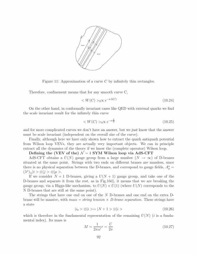
Figure 11: Approximation of a curve C by infinitely thin rectangles.

Therefore, confinement means that for any smooth curve C,

< W (C) >0∝ e−σA(C) (10.24)

On the other hand, in conformally invariant cases like QED with external quarks we findthe scale invariant result for the infintely thin curve

< W (C) >0∝ e−αTR (10.25)

and for more complicated curves we don’t have an answer, but we just know that the answermust be scale invariant (independent on the overall size of the curve).

Finally, although here we have only shown how to extract the quark antiquark potentialfrom Wilson loop VEVs, they are actually very important objects. We can in principleextract all the dynamics of the theory if we know the (complete operator) Wilson loop.

Defining the (VEV of the) N = 4 SYM Wilson loop via AdS-CFTAdS-CFT obtains a U(N) gauge group from a large number (N → ∞) of D-branes

situated at the same point. Strings with two ends on different branes are massless, sincethere is no physical separation between the D-branes, and correspond to gauge fields, Aaµ =(λa)ij |i > ⊗|j > ⊗|µ >.

If we consider N + 1 D-branes, giving a U(N + 1) gauge group, and take one of theD-branes and separate it from the rest, as in Fig.10d), it means that we are breaking thegauge group, via a Higgs-like mechanism, to U(N) × U(1) (where U(N) corresponds to theN D-branes that are still at the same point).

The strings that have one end on one of the N D-branes and one end on the extra D-brane will be massive, with mass = string tension × D-brane separation. These strings havea state

|i0 > ⊗|i >= |N + 1 > ⊗|i > (10.26)

which is therefore in the fundamental representation of the remaining U(N) (i is a funda-mental index). Its mass is

M =1

2πα′r =

U

2π(10.27)

92

This string behaves as a ”W boson,” since as the Standard Model particle, it is a vectorfield (gauge field) made massive by a Higgs mechanism, that in our case breaks U(N +1) →U(N) × U(1). The string state (or rather, its |i > endpoint) acts in the U(N) gauge theoryas a source for the U(N) gauge fields, or as a quark, and as a quark, is in the fundamentalrepresentation of U(N).

From (10.27), to get an infinite mass we need to take U → ∞. Therefore the introductionof infinitely massive external quark is obtained by having a string stretched in AdS space,in the metric (8.10), between infinity in U and a finite point.

Since infinity in (8.10) is also where the N = 4 SYM gauge theory lives, we put the Wilsonloop contour C at infinity, as a boundary condition for the string. So the string worldsheetstretches between the contour C at infinity down to a finite point in AdS, forming a smoothsurface, as in Fig.10e.

But there is a subtlety. Strings must also extend on the S5, parametrized by coordinatesθI (since the dual of N = 4 SYM is AdS5 × S5, not just AdS5). And θI correspond to thescalars XI of N = 4 SYM, which transform in the SO(6) symmetry group (R symmetry ofN = 4SYM and invariance symmetry of S5). Because of that, one finds that supersymmetrydictates that the string worldsheet described above is not a source for the usual Wilson loop,but for the supersymmetric generalized Wilson loop

W [C] =1

NTr P exp[

∮

(iAµxµ + θIXI(xµ)

√x2)dτ ] (10.28)

where xµ(τ) parametrizes the loop and θI is a unit vector that gives the position on S5 wherethe string is sitting. We will consider the case of θI =constant.

Then the prescription for calculating < W [C] > is as a partition function for the stringwith boundary on C. In the supergravity limit (gs → 0, gsN fixed and large) we obtain

< W [C] >= Zstring[C] = e−Sstring[C] (10.29)

where Sstring=string worldsheet action= 1/(2πα′)× area of worldsheet (area in AdS5 × S5,not area of the 4 dimensional projection!). That however doesn’t necessarily give the (4dimensional) area law for C, since the worldsheet has an area bigger than the 4 dimensionalarea enclosed by C.

The string has tension, and it wants to have a minimum area. In flat space, that wouldmean that it would span just the flat surface enclosed by C, giving the area law (see Fig.10f).However, in AdS space, we have a gravitational field

ds2 = α′U2

R2(−dt2 + d~x2) + ... (10.30)

To understand the physics, we compare with the Newtonian approximation (though it is nota good approximation now, but we do get the correct qualitative picture)

ds2 = (1 + 2V )(−dt2 + ...) (10.31)

where V is the Newton potential. Newtonian gravity means that the string would go to theminimum V . In our case, that would mean the minimum U . Therefore the string worldsheet

93

with boundary at U = ∞ ”drops” down to U = U0 as in Fig.10f) and is stopped (held back)by its tension.

But the prescription is not complete yet, since the area of the worldsheet stretching fromU = ∞ to U = U0 is divergent, so we would get < W [C] >= 0. In fact, we must rememberthat we said the string stretched between the |i > and |N + 1 > D-branes, and thereforebetween U = ∞ and U = U0 also represents an infinitely massive ”W boson,” whose massφ we must now subtract. The ”free W boson” would stretch along all of AdS5, thus fromU = ∞ to U = 0, in a straight line, parallel with C, as in Fig.10g. Thus the action that wemust subtract is φl, where l = length of loop C and φ = free W boson (free string) mass,U/(2π). Then

< W [C] >= e−(Sφ−lφ) (10.32)

Calculation of the quark-antiquark potentialWe take the contour C to be the infinitely thin rectangle, with T → ∞, and a quark q

at x = −L/2 and an antiquark q at x = +L/2. The metric is

ds2 = α′[U2

R2(dt2 + d~x2) +R2dU

2

U2+R2dΩ2

5]; R2 =√

4πgsN (10.33)

and the Nambu-Goto action for the string is

Sstring =1

2πα′

∫

dτdσ√

detGMN∂αXM∂βXN (10.34)

We choose a gauge where the worldsheet coordinates equal 2 spacetime coordinates,specifically τ = t and σ = x. This choice is known as a static gauge, and it is consistentto take it since we are looking for a static solution. Then we approximate the worldhseetto be translationally invariant in the time direction, which is only a good approximation ifT/L→ ∞ (otherwise the curvature of the worldsheet near the corners becomes important).Since we also are looking at a static configuration, we have a single variable for the worldsheet,U = U(σ) which becomes U = U(x).

We calculate hαβ = GMN∂αXM∂βX

N and obtain

h11 = α′U2

R2(dt

dτ)2 = α′U

2

R2; h22 = α′U

2

R2(dx

dσ)2 + α′R

2

U2(dU

dσ)2 = α′(

U2

R2+R2

U2U ′2); h12 = 0

(10.35)thus

Sstring =1

2πT

∫

dx

√

(∂xU)2 +U4

R4(10.36)

and we have reduced the problem to a 1 dimensional mechanics problem.We define U0 as the minimum of U(x) and y = U/U0. Then we can check that the

solution is defined by

x =R2

U0

∫ U/U0

1

dy

y2√

y4 − 1(10.37)

94

which gives x(U,U0) and inverted gives U(x, U0). To find U0 we note that at U = ∞ we havex = L/2, therefore

L

2=R2

U0

∫ ∞

1

dy

y2√

y4 − 1=R2

U0

√2π3/2

Γ(1/4)2(10.38)

Then from the Wilson loop prescription

Sφ − lφ = TVqq(L) (10.39)

and we regularize this formula by integrating only up to Umax. Then l ≃ 2T and the massof the string,

φ =Umax − U0

2π+U0

2π=U0

2π

∫ ymax

1

dy +U0

2π(10.40)

therefore (there is a factor of 2 since we integrate from Umax to U0 and then from U0 to Umax)

TVqq(L) = T2U0

2π[

∫ ∞

1

dy(y2

√

y4 − 1− 1) − 1] (10.41)

Finally, by substituting U0 and R2, we get

Vqq(L) = − 4π2

Γ(1/4)4

√

2g2YMN

L(10.42)

So we do get Vqq(L) ∝ 1/L as expected for a conformally invariant theory (therefore no

area law). However, we also get that Vqq(L) ∝√

g2YMN which is a nonpolynomial, therefore

nonperturbative result. That means that this cannot be obtained by a finite loop ordercalculation. For example, the 1-loop result would be proportional to g2

YMN .

Important concepts to remember

• Introducing external quarks in the theory, we can measure the quark-antiquark poten-tial between heavy sources.

• The Wilson loop, W [C] = tr P exp∫

iAµdxµ is gauge invariant.

• By choosing the contour C as a rectangle with 2 sides in the time direction, of lengthT, and two sides in a space direction, of length R ≪ T , we have a contour C fromwhich we can extract Vqq(R) by < W (C) >0= exp(−Vqq(R)).

• In a confining theory like QCD, Vqq(R) ∼ σR, thus we have the area law: < W (C) >0∝exp(−σA(C)) for any smooth curve C, and reversely, if we find the area law the theoryis confining.

• In a conformally invariant theory like QED with external quarks, Vqq(R) = α/R andthe Wilson loop is conformally (scale) invariant. For the above C, < W (C) >0∝exp(−αT/R).

95

• In AdS-CFT, the Wilson loop one finds has also coupling to scalars (and fermions),and is defined by < W (C) >0= exp(−Sstring(C)), where the string worldsheet ends atU = ∞ on the curve C and drops inside AdS space. One needs to subtract the massof the free strings extending straight down over the whole space.

• The result or the calculation is nonperturbative (proportional to√λ), but has the

expected conformal (Coulomb) behaviour.

References and further readingFor more on Wilson loops, see any QCD textbook, e.g. [39]. The Wilson loop in AdS-CFT

was defined and calculated in [40, 41]. I have followed here Maldacena’s [40] derivation.

96

Exercises, section 10

1) Check that in the nonabelian case, for a closed square contour of side a, in a planedefined by µν, we have

Φ2µν = eia2Fµν + o(a4) (10.43)

2) Check that if a free relativistic string in 4 flat dimensions is stretched between q andq and we use the AdS-CFT prescription for the Wilson loop, W [C] = e−Sstring[C], we get thearea law.

3) Consider a circular Wilson loop C, of radius R. Give an argument to show that W[C] inN=4 SYM, obtained from AdS-CFT as in the rectangular case, is also conformally invariant,i.e. independent of R.

4) Check that if AdS5 terminates at a fixed U = U1 and strings are allowed to reachU1 and get stuck there, then we get the area law for < W [C] >. (This is similar to whathappens in the case of finite temperature AdS-CFT).

5) Finish the steps left out in the calculation of the quark antiquark potential to get thefinal result for Vqq(L).

97

11 Finite temperature and scattering processes

We now turn to phenomena that have relevance for QCD, at least in terms of qualitativebehaviour. We will examine two important examples, finite temperature field theory andscattering processes.

Finite temperature in field theory; periodic timeIn quantum mechanics, we write down a transition amplitude between points q, t and

q′, t′ as

< q′, t′|q, t > = < q′|e−iH(t′−t)|q >=∑

nm

< q′|n >< n|e−iH(t′−t)|m >< m|q >

=∑

n

ψn(q′)ψ∗

n(q)e−iEn(t′−t) (11.1)

On the other hand it can also be written as a path integral

< q′, t′|q, t >=

∫

Dq(t)eiS[q(t)] (11.2)

If we perform a Wick rotation to Euclidean space by t→ −itE , t′ − t→ −iβ, iS → −SEand look at closed paths q′ = q(tE + β) = q = q(tE), we obtain

< q, t′|q, t >= Tr(e−βH) =

∫

q(tE+β)=q(tE)

Dq(tE)e−SE [q(tE)] (11.3)

That means that the Euclidean path integral on a closed path equals the statistical mechanicspartition function at temperature T = 1/β (Boltzmann constant k = 1).

Similarly in field theory we obtain for the euclidean partition function

ZE[β] =

∫

φ(~x,tE+β)=φ(~x,tE)

Dφe−SE [φ] = Tr(e−βH) (11.4)

Therefore the partition function at finite temperature T is expressed again as a euclideanpath integral over periodic euclidean time paths. One can then extend this formula byadding sources and calculating propagators and correlators, exactly as for zero temperaturefield theory.

Thus the finite temperature field theory, for static quantities only (time-independent!),is obtained by considering periodic imaginary time, with period β = 1/T .

Black hole temperatureWe can use this approach to deduce that black holes radiate thermally at a given tem-

perature T , a process known as Hawking radiation.We want to describe quantum field theory in the black hole background. As always,

it is best described by performing a Wick rotation to Euclidean time. The Wick-rotatedSchwarzschild black hole is

ds2 = +(1 − 2M

r)dτ 2 +

dr2

1 − 2Mr

+ r2dΩ22 (11.5)

98

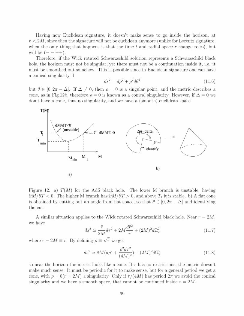
Having now Euclidean signature, it doesn’t make sense to go inside the horizon, atr < 2M , since then the signature will not be euclidean anymore (unlike for Lorentz signature,when the only thing that happens is that the time t and radial space r change roles), butwill be (−− ++).

Therefore, if the Wick rotated Schwarzschild solution represents a Schwarzschild blackhole, the horizon must not be singular, yet there must not be a continuation inside it, i.e. itmust be smoothed out somehow. This is possible since in Euclidean signature one can havea conical singularity if

ds2 = dρ2 + ρ2dθ2 (11.6)

but θ ∈ [0, 2π − ∆]. If ∆ 6= 0, then ρ = 0 is a singular point, and the metric describes acone, as in Fig.12b, therefore ρ = 0 is known as a conical singularity. However, if ∆ = 0 wedon’t have a cone, thus no singularity, and we have a (smooth) euclidean space.

2pi−delta

M

T(M)

dM/dT<0(unstable)

M

Tmin

min

T1

M1

C=dM/dT>0

a)

identify

b)

Figure 12: a) T (M) for the AdS black hole. The lower M branch is unstable, having∂M/∂T < 0. The higher M branch has ∂M/∂T > 0, and above T1 it is stable. b) A flat coneis obtained by cutting out an angle from flat space, so that θ ∈ [0, 2π − ∆] and identifyingthe cut.

A similar situation applies to the Wick rotated Schwarzschild black hole. Near r = 2M ,we have

ds2 ≃ r

2Mdτ 2 + 2M

dr2

r+ (2M)2dΩ2

2 (11.7)

where r − 2M ≡ r. By defining ρ ≡√r we get

ds2 ≃ 8M(dρ2 +ρ2dτ 2

(4M)2) + (2M)2dΩ2

2 (11.8)

so near the horizon the metric looks like a cone. If τ has no restrictions, the metric doesn’tmake much sense. It must be periodic for it to make sense, but for a general period we get acone, with ρ = 0(r = 2M) a singularity. Only if τ/(4M) has period 2π we avoid the conicalsingularity and we have a smooth space, that cannot be continued inside r = 2M .

99

Therefore we have periodic euclidean time, with period βτ = 8πM . By the previousanalysis, this corresponds to finite temperature quantum field theory at temperature

TBH =1

βτ=

1

8πM(11.9)

We can therefore say that quantum field theory in the presence of a black hole has atemperature TBH or that black holes radiate thermally at temperature TBH .

Does that mean that we can put a quantum field theory at finite temperature by addinga black hole? Not quite, since the specific heat of the black hole is

C =∂M

∂T= − 1

8πT 2< 0 (11.10)

therefore the black hole is thermodynamically unstable, and it does not represent an equi-librium situation.

But we will see that in Anti de Sitter space we have a different situation. Adding ablack hole does provide a thermodynamically stable system, which therefore does representan equilibrium situation.

Before anlyzing that however, we will try to understand better the Schwarzschild solutionin Euclidean space.

At r → ∞, the solution is R3 × S1 (since τ is periodic, but the metric is flat), which is aKaluza-Klein vacuum. That is, it is a background solution around which we can expand thefields in Fourier modes (in general, we have spherical harmonics, but for compactification ona circle we have actual Fourier modes) and perform a dimensional reduction by keeping onlythe lowest modes.

In particular, fermions can in principle acquire a phase eiα when going around the S1τ

circle at infinity:ψ → eiαψ (11.11)

These are known as ”spin structures”, and α = 0 and α = π are always OK, since theLagrangian has always terms with an even number of fermions, thus such a phase would stillleave it invariant. If L has additional symmetries, there could be other values of α allowed.

At r → 2M (the horizon), the solution is R2×S2, with R2 being dρ2+ρ2dθ2 (θ = τ/(4M))and S2 from dΩ2

2. But R2×S2 is simply connected, which means that there are no nontrivialcycles, or that any loop on R2 × S2 can be smoothly shrunk to zero. That means that therecannot be nontrivial fermion phases as you go in around any loop on R2 × S2, or that thereis a unique spin structure.

We must therefore find to what does this unique spin structure correspond at infinity?The relevant loop at infinity is τ → τ + βτ , which near the horizon is θ → θ + 2π, i.e arotation in the 2d plane R2. Under such a rotation a fermion picks up a minus sign.

Indeed, a fermion can be defined as an object that gives a minus sign under a completespatial rotation, i.e. an object that is periodic under 4π rotations instead of 2π. In 4d, theway to see that is that the spatial rotation ψ → Sψ around the axis defined by ~ν is given by

S(~ν, 0) = cosθ

2I + i~ν · ~Σ sin

θ

2; ~Σ =

(

~σ 00 ~σ

)

(11.12)

100

where ~σ are Pauli matrices. We can see that under a 2π rotation, S = −1.Therefore the unique spin strucure in the Euclidean Schwarzschild black hole background

is one that makes the fermions antiperiodic at infinity, around the Euclidean time direction.That can only happen if they have some Euclidean time dependence, ψ = ψ(θ). That inturns means that the fermions at infinity get a nontrivial mass under dimensional reductions,since the 4 dimensional free flat space equation (valid at r → ∞) gives (2 = ∂/2)

0 = 24d = (23d +∂2

∂θ2)ψ = (23d −m2)ψ (11.13)

where m2 6= 0 is a 3 dimensional spinor mass squared.Bosons on the other hand have no such restrictions on them, and we can have bosons

that are periodic at infinity under θ → θ+2π, thus also the simplest case of bosons that areindependent of θ. Then at infinity

0 = 24dφ = (23d +∂2

∂θ2)φ = 23dφ (11.14)

and therefore they can be massless in 3 dimensions.But if one would have supersymmetry in flat 3 dimensional euclidean space, we would

need that mscalar = mfermion. That is not the case in the presence of the black hole, sincewe can have mfermion 6= 0, but mboson = 0, therefore the presence of the black hole breakssupersymmetry.

In fact, one can prove that finite temperature always breaks supersymmetry, in any fieldtheory.

Therefore, one of the ways to break the unwelcome N = 4 supersymmetry in AdS-CFTand get to more realistic field theories is by having finite temperature, specifically by puttinga black hole in AdS space. We will discuss this prescrition in the following. Of course, inthe way shown above we obtain a non-supersymmetric 3 dimensional field theory, but thereare ways (that we will not explain) to obtain a 4 dimensional nonsupersymmetric theory ina similar manner.

Witten prescriptionWitten gave a prescription about how to put AdS-CFT at finite temperature by intro-

ducing a black hole in AdS5.As we have seen, the metric of global Anti de Sitter space can be written as

ds2 = −(r2

R2+ 1)dt2 +

dr2

r2

R2 + 1+ r2dΩ2 (11.15)

where in relation to the previous form in (5.22) (which was for AdS4) we have renamed1/R2 ≡ −Λ/3 (the cosmological constant Λ is < 0).

Then the black hole in (n+1)-dimensional Anti de Sitter space is

ds2 = −(r2

R2+ 1 − wnM

rn−2)dt2 +

dr2

r2

R2 + 1 − wnMrn−2

+ r2dΩ2n−2 (11.16)

101

which solves Einstein’s equation with a cosmological constant

Rµν = − n

R2gµν ≡ Λgµν (11.17)

Here

wn =16πGN

(n− 1)Ωn−1(11.18)

and Ωn−1 is the volume of the unit sphere in n − 1 dimensions. For n=3 (AdS4), Ω2 = 4πand w3 = 2GN .

Repeating the above analysis for the horizon of the Wick rotated AdS black hole, we findthat the temperature of the black hole is

T =nr2

+ + (n− 2)R2

4πR2r+(11.19)

where r+ is the largest solution of

r2

R2+ 1 − wnM

rn−2= 0 (11.20)

which is called the outer horizon. Then T(M) looks like in Fig.12a, having a minimum of

Tmin =

√

n(n− 2)

2πR(11.21)

The low M brach has C = ∂M∂T < 0 therefore is thermodynamically unstable, like theSchwarzschild black hole in flat space (it is in fact a small perturbation of that solution,since the black hole is small compared to the radius of curvature of AdS space).

The high M branch however has C = ∂M/∂T > 0, thus is thermodynamically stable.We also need to check the free energy of the black hole solution, FBH , is smaller than thefree energy of pure AdS space, FAdS.

The free energy is defined as

Z =∑

e−βF (11.22)

where β = 1/T (if k = 1). But in a gravitational theory,

Zgrav = e−S (11.23)

where S = euclidean action. We have seen this for example when defining correlators inAdS-CFT. Then we have that

S(euclidean action) =F

T(11.24)

and therefore we need to compare

FBH − FAdS = T (SBH − SAdS) (11.25)

102

and an explicit calculation shows that it is < 0 if

T > T1 =n− 1

2πR> Tmin (11.26)

There is one more problem. At r → ∞, the metric is

ds2 ≃ (r

Rdt)2 + (

R

rdr)2 + r2dΩ2

n−1 (11.27)

therefore the Euclidean time direction is a circle of radius (r/R)× (1/T ), and the transversen − 1 dimensional sphere has radius r. Thus both are proportional to r → ∞, howeverthe N = 4 SYM gauge theory that lives at r → ∞ has conformal invariance, thereforeonly relative scales are relevant for it, so we can drop the overall r. Then the topologyat infinity, where N = 4 SYM lives, is Sn−1 × S1, but we want to have a theory definedon Rn−1 × S1 instead, namely n-dimensional flat space at finite temperature (with periodicEuclidean time).

That means that we need to scale the ratio of sizes to infinity

rrR

1T

= R · T → ∞ (11.28)

Therefore we must take T → ∞, only possible if M → ∞, and we must rescale the coordi-nates to get finite quantities. The rescaling is

r =

(

wnM

Rn−2

)1/n

ρ; t =

(

wnM

Rn−2

)−1/n

τ (11.29)

and M → ∞. Under this rescaling, the metric becomes

ds2 = (ρ2

R2− Rn−2

ρn−2)dτ 2 +

dρ2

ρ2

R2 − Rn−2

ρn−2

+ ρ2n−1∑

i=1

dx2i (11.30)

and the period of τ is

β1 =4πR

n(11.31)

Since for ρ→ ∞ we get

ds2ρ→∞ ≃ ρ2(

dτ 2

R2+ d~x2) (11.32)

considering string theory in the metric (11.30)puts N = 4 SYM at constant finite tempera-ture

T =R

β1=

n

4π(11.33)

As we saw before, in this AdS black hole metric, supersymmetry is broken. At (r =)infinity, the fermions are antiperiodic around the Euclidean time direction, thus if we di-mensionally reduce the N = 4 SYM theory to 3 dimensions (compactify on the Euclidean

103

time) the fermions become massive. The gauge fields are protected by gauge invariance andremain massless under this dimensional reduction. The scalars as we saw remain masslessin 3 dimensions, at the classical level. At the quantum level, they also get a mass at 1 loop.

Therefore the 3 dimensional theory obtained by dimensionally reducing N = 4 SYM onthe compact Euclidean time is pure QCD (only gauge fields Aaµ and nothing else)! This is theperturbative spectrum of the theory, and it is defined as pure 3 dimensional QCD. But likethe real world 4 dimensional QCD, in 3 dimensions the vacuum structure is very interesting,with nonperturbative states that aquire a mass despite being composed of massless QCDfields. This phenomenon is known as a mass gap (spontaneous appearence of a minimummass of physical states in a system of massless fields).

Application: mass gapWe would like to understand the mass gap from AdS-CFT. The spontaneous appearence

of a mass for physical states of N = SYM dimensionally reduced to 3 dimensions translatesinto having a classical mass for physical states living in the gravitational dual (11.30). Wetherefore study the fields living in the bulk of the Witten metric (11.30) and we would liketo find a nonzero 3 dimensional mass (for n=4). We look for solutions of the free masslessfield equation of motion, 2φ = 0 on this space, such that

φ(ρ, ~x, τ) = f(ρ)ei~k·~x (11.34)

is independent of τ (dimensionally reduced) and factorizes in ρ and ~x dependence. At thehorizon ρ = b we need to impose that the solution is smooth, i.e. df/dρ = 0. On the otherhand, at ρ→ ∞ we need to impose that the solution is normalizable, which gives

f ∼ 1

ρ4(11.35)

There is also a non-normalizable solution that goes to a constant at infinity. Then oneplugs the ansatz and boundary conditions in the Klein-Gordon equation and finds a discretepositive spectrum of values for ~k2 ≡ m2, which is the value of the 3 dimensional masssquared. That means that the finite temperature AdS space (11.30) behaves like a quantummechanical box, with a nonzero ground state energy. This is exactly the statement of themass gap.

QCD scattering and the Polchinski-Strassler scenarioWe saw that for generic fields φ living in AdS space, they take some value φ0 on the

boundary, and then φ0 acts as a classical source for φ through

φ =

∫

KBφ0 (11.36)

and as sources for composite operators in the CFT that lives at the boundary of AdS space,out of which we can construct correlators. But in QCD we are interested in S matrices thatdescribe scattering of physical asymptotic states. The LSZ formalism relates the S matricesto correlators, but it assumes the existence of separated asymptotic states.

In a conformal field theory however, there is no notion of scale, therefore there is no notionof infinity, and no asymptotic states, so we cannot construct S matrices from correlators.

104

Therefore in order to construct S matrices so that we can study scattering of states as inQCD, we need to break the conformal invariance.

It has been understood how to modify AdS5 × S5 in order to get something closer toQCD on the field theory side. There are many examples of possible modifications. To obtainsomething that behaves like real QCD, the ”gravity dual” background looks like AdS5×X5 atlarge ρ (large fifth dimension), which describe the UV (ultraviolet or high energy) behaviourof QCD (QCD is conformal in the UV, where any small physical masses are irrelevant).Here X5 is some compact space. This AdS5 ×X5 is then modified in some way at small ρ,corresponding to the IR (infrared or low energy) behaviour of QCD.

The simplest possible model that captures some of the properties of QCD is then obtainedby just cutting off AdS5 ×X5 at a certain value of r, rmin = R2Λ, where Λ is the QCD scale(the scale of the lowest fundamental excitations).

Fields in AdS5 × X5 correspond to 4d composite operators, which correspond to gaugeinvariant, composite particles. Examples are nucleons and meson or glueballs. An exampleof glueball operator is tr FµνF

µν .The wavefunction for a glueball state, for instance eik·x, corresponds via AdS-CFT to a

wavefunction Φ for the corresponding AdS5×S5 field which equals the glueball wavefunctiontimes a wavefunction in the extra coordinates, e.g.

Φ = eik·x × Ψ(ρ, ~Ω5) (11.37)

In the example of the mass gap, this wavefunction was (11.34).Then, Polchinski and Strassler made an ansatz for the scattering of gauge invariant states

in QCD. The amplitudes A(pi) in QCD and in the ”gravity dual” are related by convolutionas

AQCD(pi) =

∫

drd5Ω√−gAstring(pi)

∏

i

Ψi(r, ~Ω) (11.38)

Since

ds2 =r2

R2d~x2 + ... (11.39)

the momentum pµ = −i∂/∂xµ is rescaled between QCD (pµ) and string theory (pµ) by

pµ =R

rpµ (11.40)

Important concepts to remember

• Finite temperature field theory is obtained by having a periodic euclidean time, withperiod β = 1/T . The partition function for such periodic paths gives the thermalpartition function, from which we can extract correlators by adding sources, etc.

• The Wick rotated Schwarzschild black hole has a smooth (non-singular) ”horizon” onlyif the euclidean time is periodic with period β = 1/TBH = 8πM . Thus black holesHawking radiate.

105

• Quantum field theory in the presence of a black hole does not have finite tempera-ture though, since the Schwarzschild black hole is thermodynamically unstable (C =∂M/∂T < 0).

• Fermions in the Wick rotated black hole are antiperiodic around the Euclidean timeat infinity, thus they are massive if we dimensionally reduce the theory on the peri-odic time. Since bosons are massless, the black hole (and finite temperature) breakssupersymmetry.

• By putting a black hole in AdS space, the thermodynamics is stable if we are at highenough black hole mass M.

• The Witten prescription for finite temperature AdS-CFT is to put a black hole of massM → ∞ inside AdS5 and to take a certain scaling of coordinates, giving the metric(11.30).

• By dimensionally reducing d=4 N = 4 Super Yang-Mills on the periodic euclideantime, we get pure Yang-Mills in 3 dimensions, which has a mass gap (spontaneousappearence of a lowest nonzero mass state in a massless theory).

• The mass gap is obtained in AdS space from solutions of the wave equation in AdS thathave a 3 dimensional mass spectrum like the one of a quantum mechanical box withthe ground state removed. Thus the Witten metric is similar in terms of eigenmodesto a finite box.

• Since N = 4 Super Yang-Mills is conformal, it does not have asymptotic states, sono S matrices. To define scattering, one must modify the duality and introduce afundamental scale (break scale invariance). The simplest model is to cut-off AdS spaceat an rmin = R2ΛQCD.

• Gauge invariant scattered states (nucleons, mesons, glueballs) correspond to fields inAdS5 × S5.

• Other models (”gravity duals”) look like AdS5 × X5 in the UV and cut-off in the IRand give theories that better mimic QCD.

• The Polchinski-Strassler scenario for the scattering amplitude of QCD (or the QCD-likemodel) is a convolution of the amplitude for scattering in the gravity dual.

References and further readingThe prescription for AdS-CFT at finite temperature was done by Witten in [42]. The

prescription for scattering of colourless states in QCD was done by Polchinski and Strasslerin [43].

106

Exercises, section 11

1) Parallel the calculation of the Schwarzschild black hole to show that the extremal(Q = M) black hole has zero temperature.

2) Derive T (r+) and Tmin(M) for the AdS black hole.

3) Check that the rescaling plus the limit given in (11.29) gives the Witten backgroundfor finite temperature AdS-CFT.

4) Take a near-horizon nonextremal D3-brane metric,

ds2 = α′U2

R2[−f(U)ds2 + d~y2] +R2 dU2

U2f(U)+R2dΩ2

5

f(U) = 1 − U4T

U4(11.41)

where UT is fixed, UT = TR2 (T=temperature). Note that for f(U) = 1 we get the near-horizon extremal D3 brane, i.e. AdS5 × S4. Check that a light ray travelling between theboundary at U = ∞ and the horizon at U = UT takes a finite time (at UT = 0, it takes aninfinite time to reach U=0).

5) Check that the rescaling

U = ρ · (TR); t =τ

TR; ~y =

~x

T(11.42)

where R = AdS radius and T=temperature, takes the above near horizon nonextremal D3brane metric to the Witten finite T AdS-CFT metric.

6) Near the boundary at r = ∞, the normalizable solutions (wavefunctions) of the massiveAdS laplaceian go like (x∆

0 ∼)r−∆ (where ∆ = 2h+ = d/2 +√

d2/4 +m2R2). Substitutein the Polchinski-Strassler formula to obtain the r dependence of the integral at large r,and using that r ∼ 1/p, estimate the hard scattering (all momenta of the same order, p)behaviour of QCD amplitudes.

107

12 The PP wave correspondence and spin chains

The Penrose limit in gravity and pp wavesPP waves are plane fronted gravitational waves that is, solutions of the Einstein equation

that correspond to perturbations moving at the speed of light, having a plane wave front.In a flat background, the pp wave metric is

ds2 = 2dx+dx− + (dx+)2H(x+, xi) +∑

i

dx2i (12.1)

For this metric, the only nonzero component of the Ricci tensor is

R++ = −1

2∂2iH(X+, xi) (12.2)

PP waves can be defined in pure Einstein gravity, supergravity, or any theory that includesgravity.

In particular, in the maximal 11 dimensional supergravity, we find a solution that hasthe above metric, together with

F4 = dx+ ∧ φ (12.3)

where φ is a 3-form that satisfies (Here ∧ denotes antisymmetrization, φ ≡ φµνρdxµ∧dxν∧dxρ,

|φ|2 ≡ φµνρφµνρ and (∗φ)µ1...µ8

≡ ǫµ1...µ11φµ9µ10µ11)

dφ = d ∗ φ = 0; ∂2iH =

1

12|φ|2 (12.4)

For φ = 0 we have a solution with

H =1

|x− x0|2(12.5)

that corresponds to a D0-brane that is localized in space and time.On the other hand, if

H =∑

ij

Aijxixj ; 2trA =

1

12|φ|2 (12.6)

we have a solution that is not localized in space and time (the spacetime is not flat at infinity).For φ = 0 we have purely gravitational solutions that obey trA = 0. A solution for generic(A, φ) preserves 1/2 of the supersymmetry, namely the supersymmetry that satisfies Γ−ǫ = 0(where ǫ is a generic supersymmetry parameter). There is however a very particular case,that has been found by Kowalski-Glikman in 1984, that preserves ALL the supersymmetry.It is

Aijxixj = −

∑

i=1,2,3

µ2

9x2i −

9∑

i=4

µ2

36x2i

φ = µdx1 ∧ dx2 ∧ dx3 (12.7)

108

He also showed that the only background solutions that preserve all the supersymmetryof 11 dimensional supergravity are Minkowski space, AdS7×S4, AdS4×S7 and the maximallysupersymmetric wave (12.7).

Observation There is one other particular type of pp wave that is relevant, the shock-wave of Aichelburg and Sexl. The solution has a delta function source, corresponding to ablack hole boosted to the speed of light (while keeping its momentum fixed), by

δn(xi, x1) → δn−1(xi)δ(x+) (12.8)

which implies that the harmonic function H of the pp wave splits as follows

H(xi, x+) = δ(x+)h(xi) (12.9)

Horowitz and Steif (1990) proved that in a pp wave background there are no α′ correctionsto the equations of motion (all possible R2 corrections vanish on-shell, i.e. by the use of theEinstein equation), therefore pp waves give exact string solutions!

In particular, 10 dimensional type IIB string theory, the theory that has AdS5 × S5 asa background solution, contains solutions of the pp wave type, with metric (12.1), togetherwith

F5 = dx+ ∧ (ω + ∗ω); H =∑

ij

Aijxixj (12.10)

satisfyingdω = d ∗ ω = 0; ; ∂2

iH = −32|ω|2 (12.11)

As in 11 dimensions, here the general metric preserves 1/2 of the supersymmetry definedby Γ−ǫ = 0. There is also a maximally supersymmetric solution, that has

H = µ2∑

i

x2i ; ω =

µ

2dx1 ∧ dx2 ∧ dx3 ∧ dx4 (12.12)

Penrose limitThere is a theorem due to Penrose, which states that near a null geodesic (the path of a

light ray) in any metric, the space becomes a pp wave.Formally, it says that in the neighbourhood of a null geodesic, we can always put the

metric in the form

ds2 = dV (dU + αdV +∑

i

βidYi) +

∑

ij

CijdYidY j (12.13)

and then we can take the limit

U = u; V =v

R2; Y i =

yi

R; R→ ∞ (12.14)

and obtain a pp wave metric in u, v, yi coordinates.The interpretation of this procedure is: we boost along a direction, e.g. x, while taking

the overall scale of the metric to infinity. The boost

t′ = cosh β t+ sinh β x; x′ = sinh β t+ cosh β x (12.15)

109

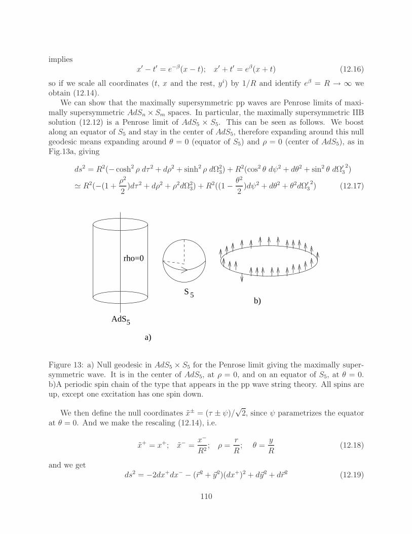
impliesx′ − t′ = e−β(x− t); x′ + t′ = eβ(x+ t) (12.16)

so if we scale all coordinates (t, x and the rest, yi) by 1/R and identify eβ = R → ∞ weobtain (12.14).

We can show that the maximally supersymmetric pp waves are Penrose limits of maxi-mally supersymmetric AdSn× Sm spaces. In particular, the maximally supersymmetric IIBsolution (12.12) is a Penrose limit of AdS5 × S5. This can be seen as follows. We boostalong an equator of S5 and stay in the center of AdS5, therefore expanding around this nullgeodesic means expanding around θ = 0 (equator of S5) and ρ = 0 (center of AdS5), as inFig.13a, giving

ds2 = R2(− cosh2 ρ dτ 2 + dρ2 + sinh2 ρ dΩ23) +R2(cos2 θ dψ2 + dθ2 + sin2 θ dΩ′

32)

≃ R2(−(1 +ρ2

2)dτ 2 + dρ2 + ρ2dΩ2

3) +R2((1 − θ2

2)dψ2 + dθ2 + θ2dΩ′

32) (12.17)

b)

rho=0

AdS

S

5

5

a)

Figure 13: a) Null geodesic in AdS5 × S5 for the Penrose limit giving the maximally super-symmetric wave. It is in the center of AdS5, at ρ = 0, and on an equator of S5, at θ = 0.b)A periodic spin chain of the type that appears in the pp wave string theory. All spins areup, except one excitation has one spin down.

We then define the null coordinates x± = (τ ± ψ)/√

2, since ψ parametrizes the equatorat θ = 0. And we make the rescaling (12.14), i.e.

x+ = x+; x− =x−

R2; ρ =

r

R; θ =

y

R(12.18)

and we getds2 = −2dx+dx− − (~r2 + ~y2)(dx+)2 + d~y2 + d~r2 (12.19)

110

which is the maximally supersymmetric wave (12.12). The F5 field also matches.Penrose limit of AdS-CFT; large R chargeSince the maximally supersymmetric wave is the Penrose limit of AdS5×S5, which defines

AdS-CFT, we would like to understand what it means to take the Penrose limit of AdS-CFT.This was done by Berenstein, Maldacena and myself (BMN) in 2002.

The energy in AdS space is given by E = i∂τ (the energy is the Noether generator oftime translations) and the angular momentum (Noether generator of rotations) for rotationsin the plane of two coordinates X5, X6 is J = −i∂ψ, where ψ is the angle between X5 andX6.

But by the AdS-CFT dictionary the energy E corresponds to the conformal dimension ∆in N = 4 SYM, whereas the angular momentum J corresponds to an R-charge, specificallya U(1) subgroup of SU(4) = SO(6) that rotates the scalar fields X5 and X6.

After taking the Penrose limit, we will have momenta p± in the pp wave backgrounddefined as

p− = −p+ = i∂x+ = i∂x+ = i(∂τ + ∂ψ) = ∆ − J

p+ = −p− = i∂x− = i∂x−

R2=

i

R2(∂t − ∂ψ) =

∆ + J

R2(12.20)

We would like to describe string theory on the pp wave, which is the Penrose limit ofAdS5 × S5. That means that we need to keep the pp wave momenta p+, p− (momenta ofphysical states on the pp wave) finite as we take the Penrose limit. That means that wemust take to infinity the radius of AdS space, R → ∞, but keep ∆ − J and (∆ + J)/R2 ofN = 4 SYM operators fixed in the limit. Therefore we must consider only SYM operatorsthat have ∆ ≃ J ∼ R2 → ∞, thus only operators with large R charge!

From the supersymmetry algebra we can obtain that ∆ ≥ |J | (in a similar manner to thecondition M ≥ |Q|, the BPS condition), which means that p± > 0. Since R2/α′ =

√gsN =

√

g2YMN , if we keep gs fixed, J ∼ R2 means that J/

√N is fixed, or we look at operators

with R-charge J ∼√N .

String spectrum from Super Yang-MillsOne can calculate the lightcone Hamiltonian (for time= x+) for a string moving in the

pp wave and obtain

Hl.c. ≡ p− = −p+ =∑

n∈Z

Nn

√

µ2 +n2

(α′p+)2(12.21)

where Nn is the total occupation number,

Nn =∑

i

ain†ain +

∑

α

bαn†bαn (12.22)

Here n > 0 are left-movers and n < 0 are right-movers. Note that the formula includesthe n=0 mode! We also have the condition that the total momentum along the closed stringshould be zero, by translational invariance (the same as for the flat space string), giving

P =∑

n∈Z

nNn = 0 (12.23)

111

A physical state is then |ni, p+ >.We note that the flat space limit µ→ 0 gives

p+p− =1

α′

∑

n

nNn (12.24)

which is indeed the flat space spectrum in lightcone parametrization (M2 = p+p− + ~p2).If we translate the Hamiltonian in SYM variables, using that E/µ = (∆ − J), p+ =

(∆ + J)/R2 ≃ 2J/R2 = 2J/(α′√

g2YMN , we get

(∆ − J)n = wn =

√

1 +g2YMN

J2(12.25)

where we are in the limit thatg2YMN

J2= fixed (12.26)

Thus we will try to find operators with fixed ∆ − J in the above limit.The SYM fieldsIn SYM J rotates X5 and X6, therefore the field Z = Φ5 + iΦ6 is charged with charge

+1 under those rotations, and Z is charged with charge −1, whereas the rest of the 6SYM scalars, φi, i = 1, ..., 4 are neutral. The gaugino χ splits under this symmetry into 8components χaJ=+1/2 and 8 components χaJ=−1/2. The 4 gauge field components Aµ completethe SYM multiplet.

These SYM fields are arranged under their gYM = 0 value for ∆ − J as follows. At∆ − J = 0 we have a single field, Z (∆ = 1 and J = 1). At ∆ − J = 1 we have Φi (∆ = 1and J = 0), χaJ=+1/2 (∆ = 3/2 and J = 1/2) and Aµ (∆ = 1 and J = 0). The rest have

∆ − J > 1 (Z and χaJ=1/2 have ∆ − J = 2).The vacuum state of the string then must be represented by an operator of momentum

p+, therefore with charge J , and with zero energy, thus with ∆ − J = 0. From the aboveanalysis, the unique such operator is

|0, p+ >=1√

JNJ/2Tr[ZJ ] (12.27)

The string oscillators (creation operators) on the pp wave at the n = 0 level are 8bosons and 8 fermions of p− = 1, therefore should correspond to fields of ∆ − J = 1 tobe inserted inside the operator corresponding to the vacuum, (12.27). They must be gaugecovariant, in order to obtain a gauge invariant operator. It is easy to see then that theunique possibility is the 8 χaJ=+1/2 for the fermions and the 4 φi’s, together with 4 covariant

derivatives DµZ = ∂µZ + [Aµ, Z] for the bosons. We have replaced the 4 Aµ’s with thecovariant derivatives DµZ in order to obtain a covariant object.

These fields are to be inserted inside the trace of the vacuum operator (12.27), for examplea state with 2 n=0 excitations will be (a†0,r corresponds to Φr and b†0,b to ψbJ=1/2)

a†0,rb†0,b|0, p+ >=

1

NJ/2+1√J

J∑

l=1

Tr[ΦrZ lψbJ=1/2ZJ−l] (12.28)

112

where we have put the φr field on the first position in the trace by cyclicity of the trace.The string oscillators at levels n > 1 are obtained in a similar manner. But now they

correspond to excitations that have a momentum einx/L around the closed string of lengthL. Since the closed string is modelled by the vacuum state Tr[ZJ ], the appropriate operatorcorresponding to an a†n,4 insertion is

a†n,4|0, p+ >=1√J

J∑

l=1

1√JNJ/2+1/2

Tr[Z lφ4ZJ−l]e2πinl

J (12.29)

Actually, this operator vanishes by cyclicity of the trace, and the corresponding string statedoesn’t satisfy the equivalent zero momentum constraint (cyclicity). In order to obtain anonzero state, we must introduce at least two such insertions.

Discretized string actionWe can now also derive a Hamiltonian that acts on the above string states, from the

SYM interactions. One starts by noting that in SYM, the operator

O = Tr[Z lφZJ−l] (12.30)

can be mapped to a state|bl >≡ Tr[(a†)lb†(a†)J−l]|0 > (12.31)

The reason this mapping can be done is a bit complicated, but one can do it. One thenperforms a rather involved derivation, which can be understood as follows. One introducesb+l operators for inserting b+ among a+’s as above. Then the action of the interacting piece ofthe Lagrangian, Lint on the 2-point function of operators O, < OO > via Feynman diagrams,becomes the action of a Hamiltonian on a state |bl >. One can then find the Hamiltonian

H ∼∑

l

b+l bl +g2YMN

(2π)2[(bl + b+l ) − (bl+1 + b+l+1)]

2 (12.32)

Then the first term is a usual harmonic oscilator, giving a discrete version of∫

dx[φ(x)2 +φ(x)2]. Since a discretized relativistic field is written as φ(x) ∼ bl + b+l , the second term is adiscretized version of φ′2, giving the continuum version of the Hamiltonian

H =

∫ L

0

dσ1

2[φ2 + φ′2 + φ2] (12.33)

where

L = J

√

π

gsN(12.34)

is the length of the string. This Hamiltonian then is exactly the Hamiltonian of the stringon a pp wave (before quantization).

This description of the insertion of φ’s and their corresponding b+l operators among aloop of Z’s and their corresponding a+ operators reminds one of spin chains. A spin chain

113

is a one dimensional system of length L of spins with only up | ↑> or down | ↓> degrees offreedom, as in Fig.13b. This equivalence can in fact be made exact.

The Heisenberg XXX spin chain Hamiltonian, HXXX

A spin chain is a model for magnetic interactions in one dimension, where the onlyrelevant degrees of freedom are the electron spins. Heisenberg (1928) wrote a simple modelfor the rotationally invariant interaction of a system of spin 1/2, called the Heisenberg XXXmodel, with Hamiltonian

H = JL∑

j=1

(~σj · ~σj+1 − 1) = 2JL∑

j=1

(Pj,j+1 − 1) (12.35)

Here ~σj are Pauli matrices (spin 1/2 operators) at site j, with periodic boundary condi-tions, i.e. ~σL+1 ≡ ~σ1, J is a coupling constant and Pi,k is the permutation operator.

• If J < 0 the system is ferromagnetic, and the interaction of spins is minimized if thespins are parallel, therefore the vacuum is | ↑↑ ... ↑>.

• If J > 0 the system is antiferromagnetic and the interaction is minimized for antipar-allel spins, therefore the vacuum is | ↑↓↑↓ ... ↑↓>.

The XXX stands for rotationally invariant. The XYZ model is not rotationally invariantand has

H =∑

j

(Jxσxj σ

xj+1 + Jyσ

yj σ

yj+1 + Jzσ

zjσ

zj+1) − const. (12.36)

and Jx 6= Jy 6= Jz.The solution of the HXXX model was done by Bethe in 1931, by what is now known as

the Bethe ansatz.Denote by |x1, ..., xN > the state with spins up at sites xi along the chain of spins down,

e.g. |1, 3, 4 >L=5= | ↑↓↑↑↓>. Each spin up excitation is called a ”magnon”.Then the one-magnon (one pseudoparticle) state is

|ψ(p1) >=

L∑

x=1

eip1x|x > (12.37)

which diagonalizes the Hamiltonian

H|ψ(p1) >= 8J sin2 p1

2|ψ(p1) >= E1|ψ(p1) > (12.38)

The ansatz for the 2-magnon state is

|ψ(p1, p2) >=∑

1≤x1<x2≤L

ψ(x1, x2) > |x1, x2 > (12.39)

where the wavefunction ψ(x1, x2) is

ψ(x1, x2) = ei(p1x1+p2x2) + S(p2, p1)ei(p2x1+p1x2) (12.40)

114

Plugging this ansatz in the Schrodinger equation we obtain solutions for S and the totalenergy E. The total energy is just the sum of the 2 magnons’ energies, E = E1 + E2, and

S(p1, p2) =φ(p1) − φ(p2) + i

φ(p1) − φ(p2) − i; φ(p) ≡ 1

2cot

p

2(12.41)

One can then also write down ansatze for a multiple magnon state, and the Schrodingerequation will give a set of equations (Bethe equations) for the ansatz, but we will not describethem here.

The SU(2) sector and HXXX from SYMIn the previous analysis we had only few insertions of b+l operators, i.e. we had only few

φi’s among mostly Z’s inside the operators and no Z’s.We can instead consider instead of such operators the ”SU(2) sector” constructed out of

two complex fields,Z = φ1 + iφ2; and W = φ3 + iφ4 (12.42)

and no φ5, φ6, nor Z and W . And consider operators with large, but arbitrary numbers ofboth Z and W , that is, operators of the type

OJ1,J2

α = Tr[ZJ1W J2] + ...(permutations) (12.43)

Then one can similarly calculate the Hamiltonian acting on states corresponding to suchoperators, and obtain that if we only consider 1-loop interactions and planar diagrams (thatcan be drawn on a plane without self-intersections; these diagrams are leading in a 1/Nexpansion, for an SU(N) gauge group),

H1−loop,planar =g2YMN

8π2HXXX1/2 (12.44)

In the notation in (12.35) we have J = −2, thus a ferromagnetic system, with groundstate | ↑↑ ... ↑>.

Important concepts to remember

• pp waves are gravitational waves (gravitational solutions for perturbations moving atthe speed of light), having a plane wave front.

• Both the maximal 11 dimensional supergravity and the 10 dimensional supergravitythat is the low energy limit of string theory have a pp wave solution that preservesmaximal supersymmetry.

• The maximally supersymmetric pp wave solution of 10 dimensional supergravity is thePenrose limit of AdS5 × S5: look near a null geodesic at ρ = θ = 0.

• The Penrose limit of AdS-CFT corresponds to large R charge J , J ≃ ∆ ∼ R2 ∼√

g2YMN .

115

• String energy levels on the pp wave are recovered from AdS-CFT if g2YMN/J

2 = fixed.String oscillators correspond to insertion of φi, DµZ and χaJ=1/2 inside Tr[ZJ ], with

some momentum e2πin/J .

• The discretized string action is obtained from Super Yang-Mills’s Feynman diagramat-tic action. Thus the long operator acts as a discretized closed string.

• The Heisenberg XXX spin chain Hamiltonian is diagonalized by Bethe ansatz, forexcitations (”magnons”) of spin up propagating in a sea of spin down states.

• One loop planar interactions in the SU(2) sector (Z,W ) of large R-charge Super Yang-Mills gives the Heisenberg XXX spin chain Hamiltonian.

References and further readingThe pp wave correspondence was defined by Berenstein, Maldacena and myself in [44]

(BMN). For a review of the correspondence, see for instance [45]. The maximally supersym-metric 11 dimensional supergravity pp wave was found by Kowalski-Glikman in [46]. TheAichelburg-Sexl shockwave was found in [47]. Horowitz and Steif [48] proved that pp wavesare solutions of string theory exact in α′. The Penrose limit can be found in [49], whereas itsphysical interpretation is described in [44]. The type IIB maximally supersymmetric planewave was found in [50] and it was shown to be the Penrose limit of AdS5 × S5 in [51, 44].The identification of the 1 loop SYM Hamiltonian with the Heisenberg spin chain was donein [52]. Good reviews of spin chain in SYM are [53, 54]. However, none of the papers andreviews for the pp wave correspondence and spin chains are easy to digest, they are at anadvanced level.

116

Exercises, section 12

1) An Aichelburg-Sexl shockwave is a gravitational solution given by a massless sourceof momentum p, i.e. T++ = pδ(x+)δ(xi). Find the function H(x+, xi) defining the pp wavein D dimensions.

2) If the null geodesic moves on S5, one can choose the coordinates such that it moveson an equator, thus the Penrose limit gives the maximally supersymmetric pp wave. Showthat if instead the null geodesic moves on AdS5, the Penrose limit gives 10d Minkowski space(choose again ρ = 0)

3) Write down the N=4 SYM fields (including derivatives) with ∆ − J = 2.

4) Check that, by cyclicity of the trace, the operator with 2 insertions of Φ1,Φ2 at levels+n and −n equals (up to normalization)

Tr[Φ1Z lΦ2ZJ−l] (12.45)

5) Check that the Bethe ansatz for 2 magnons, with

E = E1 + E2; S(p1, p2) =φ(p1) − φ(p2) + i

φ(p1) − φ(p2) − i; φ(p) =

1

2cot

p

2(12.46)

solves the Schrodinger equation for HXXX1/2.

117

13 Gravity duals

Throughout these lectures we have been dealing with the original AdS-CFT correspondence,of N = 4 Super Yang-Mills dual to string theory in AdS5×S5, since it is the best understood,and one can calculate many quantities. But since 1997, a slew of other cases have beendiscovered, including theories with less supersymmetry and/or no conformal invariance. Inthese cases (when there is no conformal field theory, and no AdS space), one can use theterm AdS-CFT, but the proper name of the correspondence is gravity-gauge duality, since itrelates a gravitational theory (string theory in a certain background) to a gauge theory in lessdimensions, via holography. In that case the gravitational background is known as the gravitydual of the gauge theory. I will try to explain some general features of these gravity-gaugedualities, explaining the map between the two theories and giving some explicit examples.

Related cases and CFTsFirst of all, there are two other cases of AdS-CFT, relating string theory in an AdS space

with a conformal field theory of maximal supersymmetry living on its boundary. Obviouslythis is not related to the same 10 dimensional type IIB string theory, since in fact there is atheorem [50] that we have aluded to in the previous section, stating that the only maximallysupersymmetric backgrounds of type IIB are 10 dimensional Minkowski space, AdS5 × S5,and the maximally supersymmetric pp wave, which is just the Penrose limit of AdS5 × S5.

They are in fact related to what is know as M-theory, which can be defined as stringtheory at a large value of the coupling gs. However, the string theory involved is type IIAstring theory, with two spinors of opposite chirality, and not the type IIB (spinors of samechirality) that we have been discussing up to now. It was shown by Witten [55] that atlarge gs, the string coupling in type IIA string theory acts as an 11-th dimension, via therelation gs = (R11/α

′)3/2. This strong coupling theory is known as M theory, and it isnot very well defined (since we don’t have a nonperturbative definition of string theory),but we do know that its low energy theory is the unique 11 dimensional supergravity. In11 dimensions, the unique spinor is made up of the 2 10 dimensional spinors of opposite10d chirality. Note that type IIB supergravity can still be related to M theory, though therelation is more complicated. For the 11 dimensional supergravity, Kowalski-Glikman [46]has shown that the only maximally supersymmetric backgrounds are 11d Minkowski space,AdS7 × S4, AdS4 × S7 and the maximally supersymmetric wave, which can be obtained asa Penrose limit of both AdS4 × S7 and AdS7 × S4.

Moreover, the AdS4 × S7 and AdS7 × S4 cases can be also obtained as the near-horizonlimit of certain brane solutions, specifically the M2- and M5-branes. Here M stands for Mtheory, which points out that these are different than D-branes: in fact, M2 can be thoughtof as a strong coupling version of a fundamental string and M5 as a strong coupling version ofa D4-brane. In any case, a similar heuristic derivation, also done by Maldacena in [29] showsthat M theory (and in particular its low energy limit, 11d supergravity) in the AdS4 × S7 /AdS7 ×S4 is dual to a certain 3 dimensional / 6 dimensional conformal field theory. Similarmethods can be used to describe these versions of AdS-CFT. The metric for AdS7 × S4 is

ds2 = l2P [U2

(πN)1/3dx2

|| + 4(πN)2/3dU2

U2+ (πN)2/3dΩ2

4] (13.1)

118

thus here Rsph = RAdS/2 = lP (πN)1/3 and the decoupling limit takes the 11 dimensionalPlanck length lP → 0, whereas the number of M5 branes N → ∞. For AdS4×S7 one obtainsRsph = 2RAdS = lP (25π2N)1/6, where lP → 0 and the number of M2 branes, N → ∞.

Conformal invariance is related to the presence of an AdS background, since as we sawthe conformal group in d Minkowski dimensions is SO(d,2), the same as the invariancegroup of AdSd+1. A number of AdS-CFT cases can be therefore obtained, but due tothe theorems mentioned above, they necessarily have less supersymmetry. Therefore wehave gauge theories in d dimensions with less supersymmetry but with conformal invariancerelated to string/M theory in a certain background of type AdSd+1 ×X. Some of these weredescribed already in [29]. Others can be obtained from the maximally supersymmetric ones(or from less supersymmetric ones) by dividing the extra space Sm (or Xm) by a discretegroup (identifying the theory under the action of a discrete subgroup of symmetries).

Indeed, the symmetry group of the extra space Xm corresponds to the ”R-symmetrygroup” of the CFTd, which itself is related to the number of supersymmetries present. Inthe case of N = 4 supersymmetry, the R-symmetry group was SU(4) = SO(6), related tothe symmetry of S5. Since dividing by a discrete subgroup will make the group of symmetriesof Xm smaller, this corresponds in the CFT with a smaller number of supersymmetries.

As an example, we will look at a conformal case with N = 2 supersymmetry involvingquarks in the fundamental representation, obtained by an ”orientifold” of AdS5×S5, analyzedin [56]. An orientifold is obtained by dividing the space by a discrete symmetry groupcomposed of a spacetime symmetry together with the worldsheet parity transformation,Xm(z, z) → Xm(z, z). The effect of worldsheet parity is to introduce some extra minus signsin the transformation laws for spacetime fields. In this model the added spacetime symmetryis a Z2 that acts on the AdS5 × S5 metric

ds2 = R2(− cosh2 ρdt2 + dρ2 + sinh2 ρdΩ23 + cos2 θdψ2 + dψ2 + sin2 θdΩ2

3)

dΩ23 = cos2 θ′dψ′2 + dψ′2 + sin2 θ′dφ2 (13.2)

as ψ′ → ψ′ + π. The effect of the orientifolding is to have θ′ ∈ (0, π/2) instead of (0, π), andthe invariant plane (”orientifold O(7) plane”) is situated at θ′ = π/2 and carries −4 units ofD7-brane charge, which are cancelled by the addition of 4 D7-branes. Due to the presence ofthe orientifold projection, the gauge group on the D3 branes (whose near horizon the abovemetric corresponds to) is not SU(N), but rather USp(2N). Then the 4 D7-branes wouldhave an SO(8) gauge symmetry on them (not SU(4) as in the absence of O(7)), but theAdS-CFT limit implies that the gauge coupling for SO(8) is zero, thus we have a model withan SO(8) global symmetry.

Strings stretching between D3-brane i and D3-brane j will have a state |i > |j > thatwould have corresponded to the adjoint of SU(N), giving the usual N = 4 Super Yang-Millsmultiplet. Due to the orientifold projection, one instead obtains the N = 2 Super Yang-Mills multiplet in the adjoint of USp(2N), coupled to a hypermultiplet in the antisymmetricrepresentation of USp(2N). Strings stretching between D7-brane m and D7-brane n willhave a state |m > |n > in the adjoint representation of SO(8), but as we mentioned,they decouple from the theory (their coupling to the rest of the fields becomes zero in theAdS-CFT limit). Finally, strings stretching between D3-brane i and D7-brane m give a

119

state |i > |m > in the fundamental representation of the gauge group USp(2N) and thefundamental of SO(8), described by hypermultiplets qm, qm, i=1,4. These can be thoughtof as N = 2 ”quarks” in the theory, which however is still conformal (as seen by the gravitydual having still an unmodified AdS5 factor).

The gravity dual is the AdS5 × S5 metric with the Z2 identification, but now the de-coupling limit still keeps the 7+1 dimensional Super Yang-Mills fields on the 7-branes atthe orientifold point. These 7-branes wrap an S3 inside the S5, thus in AdS5 we have theKaluza-Klein modes of 10d supergravity on S5, acting as usual as sources for CFT operatorsO with no SO(8) charges, but now there are also Kaluza-Klein modes of 8d SO(8) SYMfields reduced on S3, acting as sources for CFT operators Om... with SO(8) charges. Notethat these charged operators are analogous to pion operators in QCD. Indeed, the simplestsuch operator would be made up of two |i > |m > fields, in the fundamental of the gaugesymmetry USp(2N) and of the global symmetry SO(8), thus something like Omn = qmqn

(summed over gauge indices, but not global symmetry indices). For the pion we have a sim-ilar operator, with 2 quark fields, summed over SU(3) gauge indices, but not isospin SU(2)findices.

In conclusion, quarks are introduced by the addition in the dual of a different kind ofbranes (here D7 and O(7)). In the dual, it corresponds to adding Super Yang-Mills modesliving on these branes, which act as sources for pion-like operators.

Up to now the discussion was only for CFT models. When conformal invariance ispresent in the gauge field theory, therefore when we have a AdSd+1 × Xm gravity dual,we can use the same kind of methods we have described in these lectures. However wegenerically can perform less tests, since due to having less symmetries, results one one sideof the correspondence will generically get quantum corrections if the other side can be safelycalculated.

Cases without conformal invariance (and less supersymmetry)For real world applications however, we are interested in cases that break conformal

invariance as well as supersymmetry.We have seen one such example, namely putting N = 4 Super Yang-Mills at finite tem-

perature. The finite temperature broke the conformal symmetry by introducing an energyscale, the temperature T , whereas the supersymmetry was broken by the presence of an-tiperiodic boundary conditions for the fermions around the periodic euclidean time. Wesaw that Kaluza-Klein dimensional reduction of N = 4 Super Yang-Mills on the periodiceuclidean time gave us a 3 dimensional theory of pure glue (only 3d gauge fields Aaµ), whichhas a mass gap. We derived the mass gap from the fact that the gravity dual (11.30) acts asa one dimensional quantum mechanical box, with a nonzero ground state energy.

Unfortunately, in that example, the energy scale M0 characterizing the mass gap andthe masses of the discrete tower of states is proportional to the only other scale availablein the theory, the temperature scale T . However, at the scale T = 1/R we start havingback the rest of the fields of N = 4 Super Yang-Mills in 4 dimensions, instead of pure gluein 3 dimensions. This is so since the masses of Kaluza-Klein states (Fourier modes around

120

periodic time) are given by

m2einy/R = −∂2yeiny/R =

n2

R2einy/R (13.3)

so when we reach E = 1/R we cannot neglect them anymore. The fermions that weredropped out of the theory for being massive also have masses M ∝ T = 1/R. That meansthat any quantitative statements about the mass gap or massive states in 3d QCD are notquite valid anymore, since the mass scale involved is the one at which the theory is not 3dQCD anymore.

Unfortunately, this is the situation in all attempts at a QCD (or N = 1 Super QCD)gravity dual analyzed until now. One would hope that there would be a separation of scalesbetween the interesting physics scale M0 and the cut-off scale of the model (here T = 1/R),i.e. M0 ≪ T , which could in principle appear due to e.g. string coupling dependence.However, in all models studied so far, this never happens in a controllable way (such thatwe can calculate what happens).

With this caveat in mind, we will now turn to general properties of gravity duals ofinteresting field theories.

General propertiesFirst, let’s consider the ingredients available on both sides:

• A large N quantum gauge field theory. The gauge group most common is SU(N),but SO(N) or Sp(N) is also possible. In the gravity theory, N corresponds to somenumber of branes, a discrete parameter characterizing the curvature of space. We needN → ∞ to have small quantum string (gs) corrections.

• We usually want the field theory to live in flat space. This flat space can be identifiedwith the boundary at infinity of the gravity dual.

• Since we are interested in non-conformal field theories, the energy scale is relevant (thetheory does not look the same at all energy scales). The energy scale is identified withthe extra (radial) dimension of the gravity dual, whose infinity limit gives the boundaryof space. In the case of N = 4 SYM (or more precisely, for the finite temperature casewhich is non-conformal), the energy scale is U = r/α′, as we have already argued. Weobtain the so-called UV-IR correspondence: the UV of the field theory (high energiesE = U) corresponds to the IR of the gravity dual (large distances, or r → ∞), andvice versa.

• The gravity dual then is defined by the d + 1 dimensional space obtained from thefield theory space (boundary at infinity) and the energy scale, together with a compactspace Xm whose symmetries give global symmetries of the field theory.

• The nonconformal theories we are interested in are asymptotically free, which meansthey are defined in the UV. This is the meaning of the statement that the field theorylives at infinity (U → ∞) in the dual. However, since U is an energy scale, it meansthat the physics at different energy scales in the field theory correspond to physics

121

at different radial coordinates U in the gravity dual. This means that motion in Ucorresponds to RG flow in the field theory. In particular, the low energy physics (IR)of interest (since it is hard to calculate in field theory) is situated at small values of Uin the gravity dual.

Now let us define the map from field theory to gravity dual:

• The gauge group of the field theory has no correspondent in the gravity dual and onlyquantities that do not involve color indices in a nontrivial way can be calculated (e.g.correlators of gauge invariant states).

• Global symmetries in the d dimensional field theory correspond to gauge symmetriesin the d+1 dimensional space (gravity dual reduced over the compact space). Noethercurrents Jaµ for the global symmetries couple to (correspond to) gauge fields Aaµ forthose gauge symmetries in the gravity dual.

• An important special case of symmetry is Pµ (translational invariance) in the fieldtheory, whose local version is general coordinate invariance of the gravity dual. Corre-spondingly, the energy-momentum tensor Tµν (Noether current of Pµ) couples to thegraviton gµν (”gauge field of local translations”) in the gravity dual.

• As in the AdS5 × S5 case, the string coupling is gs = g2YM (this comes from the fact

that gclosed = g2open).

• Gauge invariant operators in the dual couple to (are sourced by) d + 1 dimensionalfields in the gravity dual.

• Supergravity fields in the d + 1 dimensional space (dual reduced on Xm) couple toSuper Yang-Mills operators (made of adjoint fields) in field theory (”supergravity ↔gauge field glueballs”)

• To introduce ”quarks” in the field theory (fields in the fundamental of the gauge groupand some representation of a global symmetry group G), we need to introduce SuperYang-Mills fields for the group G in the gravity dual, which couple to G-charged,pion-like operators (made of ”quarks”) in the field theory (”Super Yang-Mills ↔ pionfields”)

• Thus glueballs ↔ supergravity modes and mesons ↔ Super Yang-Mills modes.

• The mass spectrum Mn of the tower of glueballs is found as the mass spectrum for thewave equation of the correspoding supergravity mode in the gravity dual, like in theexample of AdS5 × S5 at finite temperature. A similar statement holds for mesons.

• Baryons are operators that have more than 2 fundamental fields (in QCD, there are3, in an SU(N) gauge theory there are N). They have a solitonic character in fieldtheory- they can be obtained for instance as topological solitons in the Skyrme model.The same is found in AdS-CFT: in the original AdS5 × S5 AdS-CFT, the baryon,

122

understood as a bound state of N external quarks, corresponds to a D5-brane wrappedon the S5. The same is true in more general models, the baryons being obtained insoliton-like fashion by wrapping branes on nontrivial cycles.

• Wavefunctions eik·x of states in field theory correspond to wavefunctions

Φ = eik·xΨ(U,Xm) (13.4)

of states in the gravity dual.

Finally, let us describe general features of gravity duals for QCD- or SQCD-like theories:

• At high energies, QCD or the QCD-like theories will look conformal, since all massscales become irrelevant. Therefore in the field theory UV (close to the boundary ofthe dual, U → ∞) the space will look like AdS5 × X5, with X5 some compact space,maybe with some subleading corrections to the metric.

• At low energies, QCD or the QCD-like theories are nontrivial, and have a mass gap.For AdS5 × S5, the wave equation doesn’t give a mass gap (discrete tower of massstates), a statement mapped to the fact that there is no mass gap in a CFT. Therefore,for the gravity dual of the QCD-like theory, space must terminate in a certain mannerbefore U = 0, such that the ”warp factor” U2 in front of d~x2 remains finite. In fact,since a singularity would not be good for the field theory, the space must terminate ina smooth manner. A more rigorous (though not always applicable) way to see this isas follows. It takes a finite time for a light ray to go to the boundary of AdS space,since ds2 = 0 implies

∫

dt =∫∞

dU/U2 =finite. However, it takes light an infinite timeto go to the center of AdS space, since

∫

dt =∫

0dU/U2 = ∞. Therefore if AdS space

cuts off before U = 0, as far as light is concerned, AdS space acts as a finite box, witha discrete spectrum and a mass gap (like a quantum mechanical 1d box).

• If fundamental quarks are introduced in the theory, open string modes (a gauge theory)living on a certain brane in the gravity dual must be introduced. These will couple tothe meson-like (pion-like) operators.

• If the QCD-like theory has global symmetries (like flavor symmetries or R symme-tries), they are reflected in local symmetries in the d + 1 dimensional dual theory, orequivalently in symmetries of the extra dimensional space Xm.

ExamplesLet us now exemplify the above features with some of the more used (and better defined)

models.Finite temperature reduxFirst, let us consider again AdS5 × S5 at finite temperature, since it is the simplest toy

model for pure QCD (in 3 dimensions). The metric is

ds2 = (ρ2

R2− Rn−2

ρn−2)dτ 2 +

dρ2

ρ2

R2 − Rn−2

ρn−2

+ ρ2

n−1∑

i=1

dx2i (13.5)

123

But making the rescaling r = ρ(TR)/, t = τ/(TR), ~y = ~x/T and introducing r0 = TR2 weget

ds2 =r2

R2[−dt2(1 − rn0

rn) + d~y2

(n−1)] +R2 dr2

r2(1 − rn0 /rn)

(13.6)

which is the same as the metric of the near-horizon near-extremal D3-branes. We see thatindeed at large r the metric goes over to AdS5 × S5 (in Poincare coordinates), whereas atsmall r the space terminates smoothly at r = r0. We can also check that light travels a finitetime t between r = r0 and r = ∞, and as we said the spectrum is discrete and has a massgap.

Cut-off AdS5

The simplest possible model for QCD is obtained just by cutting the AdS5 at an rmin =R2Λ. Then trivially one has that the large r metric is AdS5 × S5, and at r = rmin the spaceterminates (though not smoothly). Also trivially, light travels a finite time between r = rminand r = ∞, and the spectrum will be discrete and have the mass gap Λ, the only scale inthe theory. Therefore Λ can be phenomenologically fixed to be (related to) the mass gap.As we have described, in this simple model one can define scattering of colourless states viathe Polchinski-Strassler prescription.

But one can improve this simple model, by making the cut-off dynamical, i.e. consideringit as an added D-brane living at r = rmin in the gravity dual. By the arguments given before,the modes on this extra D-brane should source pion-like operators. In fact, it turns out thatthe fluctuation in position of this D-brane is a good enough model for (a singlet version of)the QCD pion [57]. One can in this way model the saturation of the Froissart unitaritybound for QCD from the gravity dual [58, 59, 57].

The Polchinski-Strassler solutionThe Polchinski-Strassler [60] solution gives the gravity dual of N = 1∗ SYM, which is a

certain massive deformation of N = 1 Super Yang-Mills. The brane configuration giving it isof D3 branes ”polarizing” (puffing up) into D5 branes due to the presence of a nonzero flux.It exhibits a mass gap through a phenomenon similar to the finite temperature AdS5 × S5

case (near extremal D3 branes). The metric and dilaton are given by

ds2 = Z−1/2x d~x2 + Z1/2

y (dy2 + y2dΩ2y + dw2) + Z

1/2Ω w2dΩ2

w

Zx = Zy = Z0 =R4

ρ2+ρ

2−

; ZΩ = Z0[ρ2−

ρ2− + ρ2

c

]2

ρ± = (y2 + (w ± r0)2)1/2; R4 = 4πgsN ; ρc =

2gsroα′

R2; r0 = πα′mN

e2Φ = g2s

ρ2−

ρ2− + ρ2

c

(13.7)

and m is the mass parameter of the deformation. The metric goes over to AdS5 × S5 atlarge ρ = ρ− ≃ ρ+, as it should. The ”near-core” region is ρ ∼ r0, which however is quitecomplicated (depends on y and w separately), but we see that the typical warp factor (Z1/2)is finite in this region, thus we do have the situation we advocated. At particular points,there are still AdS-like throats that are not regulated though.

124

The Klebanov-Strassler solutionThe Klebanov-Strassler solution describes an N = 1 supersymmetric SU(N + M) ×

SU(N) gauge theory (”cascading” gauge theory- at consecutive scales the relevant degreesof freedom are reduced by ”Seiberg duality” transformations, which change the descriptionto one in terms of smaller gauge groups). The metric, obtained from a configuration of M”fractional 3-branes” on a ”conifold point” (we will not explain these definitions here) in thenear horizon limit, is [61]

ds210 = h−1/2(τ)d~x2 + h1/2(τ)ds2

6

ds26 = (3/2)1/3K(τ)[

1

3K3(τ)(dτ 2 + (g5)

2) + cosh2(τ

2)((g3)

2 + (g4)2)

+ sinh2(τ

2)((g1)

2 + (g2)2)]

K(τ) =(sinh(2τ) − 2τ)1/3

21/3 sinh τ

h(τ) = α22/3

4

∫ ∞

τ

dxx coth x− 1

sinh2 x(sinh(2x) − 2x)1/3 (13.8)

and α ∝ (gsM)2 is a normalization factor. At large τ it becomes a log-corrected AdS5 ×T 1,1

metric,

ds2 = h−1/2(r)d~x2 + h1/2(r)(dr2 + r2ds2T 1,1)

h(r) ∼ (gsM)2 ln(r/rs)

r4

ds2T 11 =

1

9(dψ2 +

∑

i=1,2

cos θidφi)2 +

1

6

∑

i=1,2

(dθ2i + sin2 θidφ

2i ) =

1

9(g5)

2 +

4∑

i=1

(gi)2(13.9)

and g1, ..., g5 are some independent basis of 1-forms. Here the dilaton is approximatelyconstant, φ = φ0. Thus again, up to the log correction, we have an AdS5 ×X5 metric. Thelog correction is in fact related in this model to the log renormalization of the field theory(running coupling constant). In the field theory IR, i.e. at small τ in the gravity dual, themetric looks like

ds2 = a−1/20 d~x2 + a

1/20 (

dτ 2

2+ dΩ2

3 +τ 2

4((g1)

2 + (g2)2) (13.10)

thus here also the space terminates smoothly and the warp factor a1/20 remains finite (a0 is

a constant).The Maldacena-Nunez solutionThe solution of Maldacena and Nunez [62] involves NS5-branes wrapped on S2 (NS5-

branes can be thought of as the gs → 1/gs, or φ → −φ transformed D5-branes), givingN = 1 Super Yang-Mills in 4d, coupled to other modes. It has the (string frame) metric and

125

dilaton

ds210 = ds2

7,string + α′N1

4(wa − Aa)2

H = N [−1

4

1

6ǫabc(w

a − Aa)(wb − Ab)(wc −Ac) +1

4F a(wa − Aa)]

ds27,string = d~x2

3+1 + α′N [dρ2 +R2(ρ)dΩ22]

A =1

2[σ1a(ρ)dθ + σ2a(ρ) sinh θdφ+ σ3 cos θdφ]; a(ρ) =

2ρ

sinh 2ρ

R2(ρ) = ρ coth(2ρ) − ρ2

sinh2(2ρ)− 1

4

e2φ = e2φ02R(ρ)

sinh(2ρ)(13.11)

where the first two lines represent the uplifting of a 7d N = 1 supergravity solution into10d on S3 (transverse to the 5-branes), the rest represent the 7d solution and wa are left-invariant one-forms on S3. However, the decoupling of other modes (Kaluza-Klein modes,for instance) cannot be done in a controllable way, as usual (to do so one needs to switch toa D5-brane description, that is highly nonperturbative).

The behaviour at ρ→ ∞ (corresponding to the usual UV boundary of space) is

R2 ∼ ρ; a ∼ 2ρe−2ρ; φ = φ0 − ρ+log ρ

4(13.12)

At first, it seems this is not good, since we do not obtain a log-corrected AdS5 × X5

space, but rather

ds2 = d~x23+1 + α′N [dρ2 + ρdΩ2

2 +1

4(wa −Aa)2]

= d~x23+1 + α′N [

dz2

z2+ (− log z)dΩ2

2 +1

4(wa − Aa)2] (13.13)

where ρ = − log z. However, now the dilaton is nontrivial, unlike the previous cases (andunlike for AdS5). But in fact, this is good, since all we need is that the 5 dimensionalKaluza-Klein reduced supergravity action is the same. In the presence of a dilaton (andusing a ”string frame” metric as above), the relevant action is

S =

∫

d5x√g5

(∫

X5

√gX5

)

e−2φ[R + (∂X)2 + ...]

=

∫

d5x√g5

(∫

X5

√gX5

)

gµνe−2φ[Rµν + ∂µX∂νX + ...] (13.14)

where X is a generic scalar. For a metric

ds2 = e2A(ρ)d~x23+1 + dρ2 + ds2

X5= e2A(z)d~x2

3+1 +dz2

z2+ ds2

X5(13.15)

126

the bracket [Rµν + ∂µX∂νX + ...] doesn’t contain e2A factors and we get

∫

d4xdρ

(∫

X5

√gX5

)

e2(A−φ)δµν [Rµν + ∂µX∂νX + ...] (13.16)

thus in fact we have the condition

φ− φ0 −Aρ→∞→ −ρ(+ log corrections) = + log z(+ corrections) (13.17)

which before was satisfied by φ = φ0 and A→ −ρ+ ... = + log z+ ..., but now is satisfied byA = 0 and φ = φ0 − ρ+ ... = φ0 + log z+ .... Also note that now there is some ρ dependencein

√gX5

as well.The behaviour in the IR of the field theory, i.e. at ρ→ 0 is

R2 = ρ2 + o(ρ4); a = 1 + o(ρ2); φ = φ0 + o(ρ2) (13.18)

which means that the effective warp factor e2(A−φ) is constant as in the previous examples.The Maldacena-Nastase solutionThe Maldacena-Nastase solution in [63] is the analog of the Maldacena-Nunez solution

for NS5-branes wrapped on S3, and gives N = 1 Super Yang-Mills in 3 dimensions, with aChern-Simons coupling, and coupled to other modes as in 4d. The Chern-Simons couplingis quantized as always by a quantum number k. The gravity dual corresponds to k = N/2,where N is the number of 5-branes, and in this case an index computation shows that thereis a unique vacuum, that confines. The solution is

ds210 = ds2

7,string + α′N1

4(wa − Aa)2

H = N [−1

4

1

6ǫabc(w

a − Aa)(wb − Ab)(wc −Ac) +1

4F a(wa − Aa)] + h

ds27,string = d~x2

2+1 + α′N [dρ2 +R2(ρ)dΩ23]

A =w(ρ) + 1

2waL

h = N [w3(ρ) − 3w(ρ) + 2]1

16

1

6ǫabcw

awbwc

(13.19)

where w(ρ), R(ρ), φ(ρ) have some complicated form that can be evaluated numerically. Atlarge ρ they become

R2(ρ) ∼ 2ρ; w(ρ) ∼ 1

4ρ; φ = −ρ+

3

8log ρ (13.20)

thus as for the Maldacena-Nunez solution,

φ− φ0 −A→ −ρ+ log corrections (13.21)

127

where the metric is

ds2 = e2A(ρ)d~x22+1 + dρ2 + ds2

X6= e2A(z)d~x2

2+1 +dz2

z2+ ds2

X6(13.22)

implying the same dual supergravity action as in a log-corrected AdS4 ×X6 background.The behaviour at ρ→ 0 (for the IR of the field theory) is

R2(ρ) = ρ2 + o(ρ4); w(ρ) = 1 + o(ρ2); φ = φ0 + o(ρ2) (13.23)

giving a finite effective warp factor, e2(A−φ) = e−2φ0+....If we wrap a small number n of branes (n ≪ N/2) on a non-contractible S3 in the

geometry, the metric is unmodified, but the dual field theory is modified by having k = N/2+n, that still preserves supersymmetry. By adding |n| (n < 0) antibranes instead, we get k =N/2 + n which breaks supersymmetry dynamically. Thus this dynamical (nonperturbative)breaking of supersymmetry becomes a spontaneous (classical) effect in field theory, anothergood example of the power of AdS-CFT.

The Sakai-Sugimoto modelThe Sakai-Sugimoto model [64] is a model that incorporates quarks (fermions in the fun-

damental representation of the gauge group), however does so in a probe approximation, i.e.without incorporating the backreaction of the modes dual to quark operators to the geom-etry. Specifically, the model involves a large number Nc of D4 branes at finite temperaturegiving a gravity dual similar to the one studied by Witten for D3-branes, namely

ds2 =

(

U

R

)3/2

(f(U)dτ 2 + d~x2) +

(

R

U

)3/2

(dU2

f(U)+ U2dΩ2

4)

eφ = gs

(

U

R

)3/4

; F4 =2πNc

V4ǫ4; f(U) = 1 − U3

KK

U3(13.24)

Inside this background, one considers Nf D8-brane probes, whose transverse coordinate isU , and is value depends on the worldvolume coordinate τ , i.e. U = U(τ). The solution forU(τ) is given via its inverse,

τ(U) = U40 f(U0)

1/2

∫ U

U0

dU

(UR)3/2f(U)

√

U8f(U) − U80 f(U0)

(13.25)

The modes living on this brane are dual to (couple to) mesonic operators (pion-like, involvingquarks and charged under the global symmetry). Unlike e.g. the CFT dual in [56], thebackreaction of this modes on the geometry has not been included, i.e. the backgroundmetric is not modified by the presence of the D8-branes. That means that the model is validonly perturbatively if Nf ≪ Nc, otherwise one has corrections to this solution.

The D4 brane background at finite temperature is similar to the Witten constructionfor D3 branes at finite temperature (giving N = 4 SYM at finite temperature). In fact,in [42] it was related to a construction of pure 4 dimensional SU(N) Yang-Mills via sometransformations and compactification on periodic euclidean time. We can easily see that up

128

to a overall (conformal) factor, the metric has the right behaviour, by changing variables toρ = U1/2, which gives the metric

ds2 = ρ

[

ρ2(f(ρ)dτ 2 + d~x2) +dρ2

f(ρ)ρ2+ dΩ2

4

]

(13.26)

So up to a conformal factor, we get AdS6 × S4 at large U . Compactification on τ givesthe correct behaviour for the dual of the 4 dimensional theory.

Finite N?Throughout these lectures we have analyzed only large N (N → ∞) gauge theories, and

one can treat perturbations away from N = ∞ by including string (gs) corrections. But forthe case of interest, namely real QCD, N = 3 which is far from infinity. However, it is knownthat for most quantities of interest, corrections are actually of order 1/N2 ≃ 0.1, which canbe argued to be small. But one would like to know whether we can calculate anything atfinite N , and perhaps at finite λ = g2

YMN (which corresponds to string worldsheet (α′)corrections). For generic quantities, the answer (at this point) is no.

However, there is one process for which this is possible, namely forward (small angle)scattering of gauge invariant particles. It was shown in [58, 59] that string corrections (bothworldsheet α′ and quantum gs corrections) to the high energy, small angle (forward, or inthe case of 4-point scattering s → ∞ and t fixed) scattering cross section in a gravitationaltheory are exponentially small in the energy, specifically

exp(− G24s

8α′ log(α′s)) (13.27)

From this we can calculate, using the Polchinski-Strassler formalism described in section 11,that 1/N and 1/(g2N) corrections to the high energy small angle scattering cross section areexponentially suppressed in energy.

129

References

[1] M. E. Peskin and D. V. Schroeder, ”An introduction to quantum field theory,” PerseusBooks, 1995.

[2] Steven Weinberg, ”The quantum theory of fields,” vols. 1,2,3, Cambridge UniversityPress, 1995, 1996 and 2000.

[3] P. J. E. Peebles, ”Principles of physical cosmology,” Princeton University Press, 1993.

[4] C. W. Misner, K. S. Thorne and J. A. Wheeler, ”Gravitation,” W. H. Freeman and Co.,1970

[5] L.D. Landau and E. M. Lifchitz, ”Mechanics,” Butterworth-Heinemann, 1982.

[6] R. M. Wald, ”General relativity,” University of Chicago Press, 1984.

[7] S. V. Ketov, ”Solitons, monopoles and duality: from sine-Gordon to Seiberg-Witten,”Fortsch. Phys. 45 (1997) 237 [arXiv:hep-th/9611209].

[8] L. Alvarez-Gaume, S. F. Hassan, ” Introduction to S-duality in N=2 supersymmetricgauge theory. (A pedagogical review of the work of Seiberg and Witten),” Fortsch. Phys.45 (1997) 159 [arXiv:hep-th/9701069].

[9] P. West, ”Introduction to supersymmetry and supergravity,” World Scientific, 1990.

[10] J. Wess and J. Bagger, ”Supersymmetry and supergravity,” Princeton University Press,1992.

[11] S. J. Gates, M. T. Grisaru, M. Rocek and W. Siegel, ”Superspace or one thousand andone lessons in supersymmetry,” Front. Phys. 5 (1983) 1 [arXiv:hep-th/0108200]

[12] M. Dine, ”Supersymmetry and string theory, Beyond the Standard Model,” CambridgeUniversity Press, 2007.

[13] P. van Nieuwenhuizen, Les Houches 1983, Proceedings, Relativity, groups and topologyII, p. 823.

[14] P. van Nieuwenhuizen, ”Supergravity,” Phys. Rept. 68 (1981) 189.

[15] M. J. Duff, B. E. W. Nilsson and C. N. Pope, ”Kaluza-Klein supergravity,” Phys. Rept.130 (1986) 1.

[16] S. W. Hawking and G. F. R. Ellis, ”The large scale structure of space-time,” CambridgeUniversity Press, 1973.

[17] M. J. Duff, R. R. Khuri and J. X. Lu, ”String solitons,” Phys. Rept. 259 (1995) 213[arXiv:hep-th/9412184].

130

[18] A. A. Tseytlin, ”Harmonic superpositions of M-branes,” Nucl. Phys. B475 (1996) 149[arXiv:hep-th/9604035]

[19] M. Cvetic, A. A. Tseytlin, ”Non-extreme black holes from non-extreme intersectingM-branes,” Nucl. Phys. B478 (1996) 181 [arXiv:hep-th/9606033]

[20] B. Zwiebach, ”A first course in string theory,” Cambridge University Press, 2004.

[21] M. B. Green, J. H. Schwarz and E. Witten, ”Superstring theory,” vols. 1 and 2, Cam-bridge University Press, 1987.

[22] Joseph Polchinski, ”String theory”, vol.1 and 2, Cambridge University Press, 1998.

[23] K. Becker, M. Becker and J. H. Schwarz, ”String theory and M-theory,” CambridgeUniversity Press, 2007.

[24] Clifford Johnson, ”D-branes,” Cambridge University Press, 2003.

[25] O. Aharony, S. S. Gubser, J. Maldacena, H. Ooguri and Y. Oz, ”Large N field theories,string theory and gravity,” Phys. Rept. 323 (2000) 183 [arXiv:hep-th/9905111]

[26] J. Dai, R. G. Leigh and J. Polchinski, ”New connections between string theories,” Mod.Phys. Lett. A4 (1989) 2073

[27] J. Polchinski, ”Dirichlet branes and Ramond-Ramond charges,” Phys. Rev. Lett. 75(1995) 4724 [arXiv:hep-th/9510017]

[28] E. D’Hoker and D. Z. Freedman, ”Supersymmetric gauge theories and the AdS/CFTcorrespondence,” TASI 2001 lecture notes, arXiv:hep-th/0201253.

[29] J. M. Maldacena, ”The large N limit of superconformal field theories and supergrav-ity,” Adv. Theor. Math. Phys. 2 (1998) 231; Int. J. Theor. Phys. 38 (1999) 1113[arXiv:hep-th/9711200]

[30] S. S. Gubser, I. R. Klebanov, A. M. Polyakov, ”Gauge theory correlators from non-critical string theory,” Phys. Lett. B428 (1998) 105 [arXiv:hep-th/9802109].

[31] E. Witten, ”Anti de Sitter space and holography,” Adv. Theor. Math. Phys. 2 (1998)253 [arXiv:hep-th/9802150]

[32] H. J. Kim, L. J. Romans and P. van Nieuwenhuizen, ”The mass spectrum of chiral N=2D=10 supergravity on S5,” Phys. Rev. D32 (1985) 389.

[33] B. de Wit and H. Nicolai, Nucl. Phys. B 243 (1984) 91; B. de Wit, H. Nicolai andN. P. Warner Nucl. Phys. B 255 (1985) 29; B. de Wit, H. Nicolai, Nucl. Phys. B 274(1986) 363; B. de Wit, H. Nicolai, Nucl. Phys. B 281 (1987) 211

131

[34] H. Nastase, D. Vaman and P. van Nieuwenhuizen, ”Consistent nonlinear KK reductionof 11d supergravity on AdS7×S4 and self-duality in odd dimensions,” Phys. Lett. B469(1999) 96 [arXiv:hep-th/9905075]

[35] H. Nastase, D. Vaman and P. van Nieuwenhuizen, ”Consistency of the AdS7 × S4 re-duction and the origin of self-duality in odd dimensions,” Nucl. Phys. B581 (2000) 179[arXiv:hep-th/9911238].

[36] W. Muck and K. S. Viswanathan, ”Conformal field theory correlators from classicalscalar field theory on AdSd+1,” Phys. Rev. D58 (1998) 041901 [arXiv:hep-th/9804035].

[37] D. Z. Freedman, S. D. Mathur, A. Matusis and L. Rastelli, ”Correlation func-tions in the CFT(d)/AdS(d+1) correpondence,” Nucl. Phys. B546 (1999) 96[arXiv:hep-th/9804058].

[38] G. Chalmers, H. Nastase, K. Schalm and R. Siebelink, ”R-Current correlators in N=4Super Yang-Mills theory from Anti-de Sitter supergravity,” Nucl. Phys. B540 (1999)247 [arXiv:hep-th/9805105].

[39] A. Smilga, ”Lectures on Quantum Chromodynamics,” World Scientific, 2001.

[40] J. M. Maldacena, ”Wilson loops in large N field theories,” Phys. Rev. Lett. 80 (1998)4859 [arXiv:hep-th/9803002]

[41] S.-J. Rey and J.-T. Yee, ” Macroscopic strings as heavy quarks: Large-N gauge theoryand anti-de Sitter supergravity,” Eur. Phys. J. C22 (2001) 379 [arXiv:hep-th/9803001]

[42] E. Witten, ”Anti-de Sitter space, thermal phase transition, and confinement in gaugetheories,” Adv. Theor. Math. Phys. 2 (1998) 505 [arXiv:hep-th/9803131]

[43] J. Polchinski and M. J. Strassler, ”Hard scattering and gauge/string duality,” Phys.Rev. Lett. 88 (2002) 031601 [arXiv:hep-th/0109174]

[44] D. Berenstein, J. M. Maldacena and H. Nastase, ”Strings in flat space and pp wavesfrom N = 4 Super Yang Mills,” JHEP 0204 (2002) 013 [arXiv:hep-th/0202021]

[45] Jan Plefka, ”Lectures on the plane-wave string/gauge theory duality,” Fortsch. Phys.52 (2004) 264 [arXiv:hep-th/0307101].

[46] J. Kowalski-Glikman, ”Vacuum States In Supersymmetric Kaluza-Klein Theory,” Phys.Lett. B 134, 194 (1984).

[47] P. C. Aichelburg and R. U. Sexl, ”On the gravitational field of a massless particle,”Gen. Rel. and Grav. 2 (1971) 303.

[48] G. T. Horowitz and A. R. Steif, ”Space-Time Singularities In String Theory,” Phys.Rev. Lett. 64, 260 (1990).

132

[49] R. Penrose, ”Any spacetime has a plane wave as a limit,” Differential geometry andrelativity, Reidel, Dordrecht, 1976, pp. 271-275.

[50] M. Blau, J. Figueroa-OFarrill, C. Hull and G. Papadopoulos, ”A new maximallysupersymmetric background of IIB superstring theory,” JHEP 0201, 047 (2001)[arXiv:hep-th/0110242].

[51] M. Blau, J. Figueroa-O’Farrill, C. Hull and G. Papadopoulos, ”Penrose limits andmaximal supersymmetry,” Class. Quant. Grav. 19 (2002) L87 [arXiv:hep-th/0201081].

[52] J. A. Minahan and K. Zarembo, ”The Bethe-Ansatz for N=4 Super Yang-Mills,” JHEP0303 (2003) 013 [arXiv:hep-th/0212208]

[53] Jan Plefka, ”Spinning strings and integrable spin chains in the AdS-CFT correspon-dence,” hep-th/0507136

[54] K. Zarembo, ”Semiclassical Bethe ansatz and AdS-CFT,” Comptes Rendus Physique 5(2004) 1081 and Fortsch. Phys. 53 (2005) 647 [arXiv:hep-th/0411191].

[55] E. Witten, ”String theory dynamics in various dimensions,” Nucl. Phys. B443 (1995)85 [arXiv:hep-th/9503124]

[56] O. Aharony, A. Fayyazuddin and J. Maldacena, ”The Large N limit of N = 2, 1 fieldtheories from threebranes in F-theory,” JHEP 9807 (1998) 013 [arXiv:hep-th/9806159].

[57] S. B. Giddings, ”High energy QCD scattering, the shape of gravity on an IR brane, andthe Froissart bound,” Phys. Rev. D67 (2003) 126001 [arXiv:hep-th/0203004]

[58] K. Kang and H. Nastase, ”High energy QCD from Planckian scattering in AdS and theFroissart bound,” Phys.Rev. D72 (2005) 106003 [arXiv:hep-th/0410173]

[59] K. Kang and H. Nastase, ”Heisenberg saturation of the Froissart bound from AdS-CFT,” Phys. Lett. B624 (2005) 125 [arXiv:hep-th/0501038]

[60] J. Polchinski and M. J. Strassler, ”The string dual of a confining four-dimensional gaugetheory,” arXiv:hep-th/0003136.

[61] I. Klebanov and M. J. Strassler, ”Supergravity and a confining gauge theory: Du-ality cascades and chi SB resolution of naked singularities,” JHEP 0008 (2000) 052[arXiv:hep-th/0007191].

[62] J. M. Maldacena and C. Nunez, ”Towards the large N limit of pure N=1 super Yang-Mills,” Phys. Rev. Lett. 86 (2001) 588 [arXiv:hep-th/0008001]

[63] J. M. Maldacena and H. Nastase, ”The supergravity dual of a theory with dynamicalsupersymmetry breaking,” JHEP 0109 (2001) 024 [arXiv:hep-th/0105049]

[64] T. Sakai and S. Sugimoto, ”Low energy hadron physics in holographic QCD,” Prog.Theor. Phys. 113 (2005) 843 [arXiv:hep-th/0412141]

133