OU-HET-961

Deep Learning and AdS/CFT

Koji Hashimoto,1 Sotaro Sugishita,1 Akinori Tanaka,2, 3, 4 and Akio Tomiya5

1Department of Physics, Osaka University, Toyonaka, Osaka 560-0043, Japan2Mathematical Science Team, RIKEN Center for Advanced Intelligence Project (AIP),

1-4-1 Nihonbashi, Chuo-ku, Tokyo 103-0027, Japan3Department of Mathematics, Faculty of Science and Technology,

Keio University, 3-14-1 Hiyoshi, Kouhoku-ku, Yokohama 223-8522, Japan4interdisciplinary Theoretical & Mathematical Sciences Program

(iTHEMS) RIKEN 2-1, Hirosawa, Wako, Saitama 351-0198, Japan5Key Laboratory of Quark & Lepton Physics (MOE) and Institute of Particle Physics,

Central China Normal University, Wuhan 430079, China

We present a deep neural network representation of the AdS/CFT correspondence, and demon-strate the emergence of the bulk metric function via the learning process for given data sets ofresponse in boundary quantum field theories. The emergent radial direction of the bulk is identifiedwith the depth of the layers, and the network itself is interpreted as a bulk geometry. Our net-work provides a data-driven holographic modeling of strongly coupled systems. With a scalar φ4

theory with unknown mass and coupling, in unknown curved spacetime with a black hole horizon,we demonstrate our deep learning (DL) framework can determine them which fit given responsedata. First, we show that, from boundary data generated by the AdS Schwarzschild spacetime, ournetwork can reproduce the metric. Second, we demonstrate that our network with experimentaldata as an input can determine the bulk metric, the mass and the quadratic coupling of the holo-graphic model. As an example we use the experimental data of magnetic response of a stronglycorrelated material Sm0.6Sr0.4MnO3. This AdS/DL correspondence not only enables gravity mod-eling of strongly correlated systems, but also sheds light on a hidden mechanism of the emergingspace in both AdS and DL.

Introduction.— The AdS/CFT correspondence [1–3], arenowned holographic relation between d-dimensionalquantum field theories (QFTs) and (d + 1)-dimensionalgravity, has been vastly applied to strongly coupled QFTsincluding QCD and condensed matter systems. For phe-nomenology, the holographic modelings were successfulonly for restricted class of systems in which symmetriesare manifest, mainly because the mechanism of how theholography works is still unknown. For a quantum sys-tem given, we do not know whether its gravity dual existsand how we can construct a holographic model.

Suppose one is given experimental data of lin-ear/nonlinear response under some external field, canone model it holographically? In this letter we employdeep learning (DL) [4–6], an active subject of compu-tational science, to provide a data-driven holographicgravity modeling of strongly coupled quantum systems.While conventional holographic modeling starts with agiven bulk gravity metric, our novel DL method solvesthe inverse problem: given data of a boundary QFT cal-culates a suitable bulk metric function, assuming the ex-istence of a black hole horizon.

Our strategy is simple: we provide a deep neural net-work representation of a scalar field equation in (d+ 1)-dimensional curved spacetime. The discretized holo-graphic (“AdS radial”) direction is the deep layers, seeFig. 1. The weights of the neural network to be trainedare identified with a metric component of the curvedspacetime. The input response data is at the boundaryof AdS, and the output binomial data is the black hole

FIG. 1: The AdS/CFT and the DL. Top: a typical view of theAdS/CFT correspondence. The CFT at a finite temperaturelives at a boundary of asymptotically AdS spacetime with ablack hole horizon at the other end. Bottom: a typical neuralnetwork of a deep learning.

horizon condition. Therefore, a successful machine learn-ing results in a concrete metric of a holographic modelingof the system measured by the experiment [67]. We callthis implementation of the holographic model into thedeep neural network as AdS/DL correspondence.

We check that the holographic DL modeling nicely

arX

iv:1

802.

0831

3v1

[he

p-th

] 2

2 Fe

b 20

18

2

works with the popular AdS Schwarzschild metric, byshowing that the metric is successfully learned and re-produced by the DL. Then we proceed to use an exper-imental data of a magnetic response of Sm0.6Sr0.4MnO3

known to have strong quantum fluctuations, and demon-strate the emergence of a bulk metric via the AdS/DLcorrespondence.

Our study gives a first concrete implementation of theAdS/CFT into deep neural networks. We show the emer-gence of a smooth geometry from given experimentaldata, which opens a possibility of revealing the mysteryof the emergent geometry in the AdS/CFT with the helpof the active researches of DL. A similarity between theAdS/CFT and the DL was discussed recently [7] [68],and it can be discussed through tensor networks, theAdS/MERA correspondence [11] [69].

Let us briefly review a standard deep neural network.It consists of layers (see Fig. 1), and between the adja-cent layers, a linear transformation xi → Wijxj and anonlinear transformation known as an activation func-tion, xi → ϕ(xi), are succeedingly act. The final layer isfor summarizing all the component of the vector. So theoutput of the neural network is

y(x(1)) = fiϕ(W(N−1)ij ϕ(W

(N−2)jk · · ·ϕ(W

(1)lm x(1)

m ))). (1)

In the learning process, the variables of the network

(fi,W(n)ij ) for n = 1, 2, · · · , N − 1 are updated by a gra-

dient descent method with a given loss function of theL1-norm error,

E ≡∑data

∣∣∣∣ y(x(1))− y∣∣∣∣ +Ereg(W ). (2)

Here the sum is over the whole set of pairs {(x(1), y)} ofthe input data x(1) and the output data y. The regular-ization Ereg is introduced to require expected propertiesfor the weights [70].

Neural network of scalar field in AdS.— Let us embed thescalar field theory into a deep neural network. A scalarfield theory in a (d+ 1)-dimensional curved spacetime iswritten as

S=

∫dd+1x

√−det g

[−1

2(∂µφ)2 − 1

2m2φ2 − V (φ)

].

(3)

For simplicity we consider the field configuration to de-pend only on η (the holographic direction). Here thegeneric metric is given by

ds2 = −f(η)dt2 + dη2 + g(η)(dx21 + · · ·+ dx2

d−1) (4)

with the asymptotic AdS boundary condition f ≈ g ≈exp[2η/L] (η ≈ ∞) with the AdS radius L, and anotherboundary condition at the black hole horizon, f ≈ η2, g ≈

FIG. 2: The simplest deep neural network reproducingthe homogeneous scalar field equation in a curved spacetime.Weights W are shown by solid lines explicitly, while the acti-vation is not.

const. (η ≈ 0). The classical equation of motion for φ(η)is

∂ηπ + h(η)π −m2φ− δV [φ]

δφ= 0, π ≡ ∂ηφ , (5)

where we have defined π so that the equations become afirst order in derivatives. The metric dependence is sum-marized into a combination h(η) ≡ ∂η log

√f(η)g(η)d−1.

Discretizing the radial η direction, the equations arerewritten as

φ(η + ∆η) = φ(η) + ∆η π(η) , (6)

π(η + ∆η) = π(η)−∆η

(h(η)π(η)−m2φ(η)− δV (φ)

δφ(η)

).

We regard these equations as a propagation equationon a neural network, from the boundary η = ∞ wherethe input data (φ(∞), π(∞)) is given, to the black holehorizon η = 0 for the output data, see Fig. 2. TheN layers of the deep neural network are a discretizedradial direction η which is the emergent space in AdS,

η(n) ≡ (N −n+ 1)∆η. The input data x(1)i of the neural

network is a two-dimensional real vector (φ(∞), π(∞))T.So the linear algebra part of the neural network (the solidlines in Fig. 1) is automatically provided by

W (n) =

(1 ∆η

∆ηm2 1−∆η h(η(n))

). (7)

The activation function at each layer reproducing (6) is{ϕ(x1) = x1,

ϕ(x2) = x2 + ∆η δV (x1)δx1

.(8)

The definitions (7) and (8) bring the scalar field system incurved geometry (3) into the form of the neural network(1) [71].

Response and input/output data.— In the AdS/CFT,asymptotically AdS spacetime provides a boundary con-dition of the scalar field corresponding to the responsedata of the quantum field theory (QFT). With the AdSradius L, asymptotically h(η) ≈ d/L. The external fieldvalue J (the coefficient of a non-normalizable mode of φ)and its response 〈O〉 (that of a normalizable mode) in

3

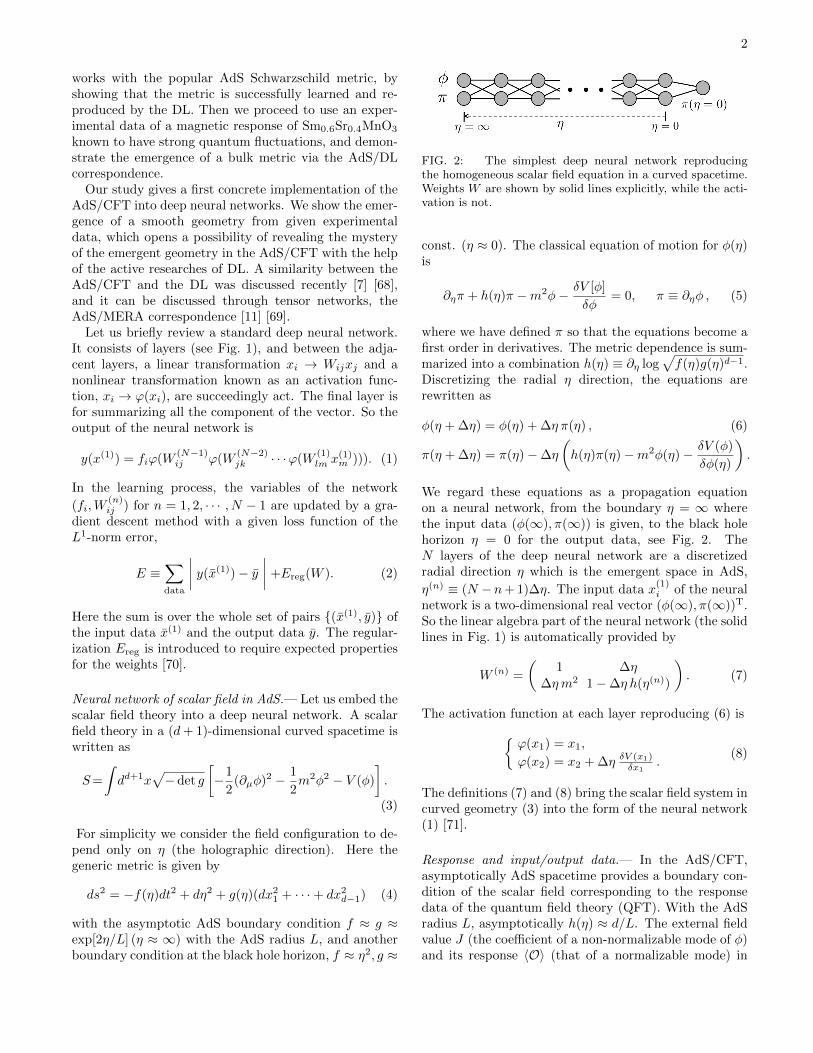
FIG. 3: The data generated by the discretized AdSSchwarzschild metric (11). Blue points are the positive data(y = 0) and the green points are the negative data (y = 1).

the QFT are [55], in the unit of L = 1, a linear map

φ(ηini) = J exp[−∆−ηini] + 〈O〉exp[−∆+ηini]

∆+ −∆−, (9)

π(ηini) = −J∆− exp[−∆−ηini]− 〈O〉∆+ exp[−∆+ηini]

∆+ −∆−,

with ∆± ≡ (d/2)±√d2/4 +m2L2 (∆+ is the conformal

dimension of the QFT operator O corresponding to thebulk scalar φ). The value η = ηini ≈ ∞ is the regularizedcutoff of the asymptotic AdS spacetime. We use (9) forconverting the response data of QFT to the input dataof the neural network.

The input data at η = ηini propagates in the neuralnetwork toward η = 0, the horizon. If the input datais positive, the output at the final layer should satisfythe boundary condition of the black hole horizon (see forexample [56]),

0 = F ≡[

2

ηπ −m2φ− δV (φ)

δφ

]η=ηfin

(10)

Here η = ηfin ≈ 0 is the horizon cutoff. Our final layeris defined by the map F , and the output data is y = 0for a positive answer response data (J, 〈O〉). In the limitηfin → 0, the condition (10) is equivalent to π(η = 0) = 0.

With this definition of the network and the trainingdata, we can make the deep neural network to learn themetric component function h(η), the parameter m andthe interaction V [φ]. The training is with a loss functionE given by (2)[72]. Experiments provide only positiveanswer data {(J, 〈O〉), y = 0}, while for the training weneed also negative answer data : {(J, 〈O〉), y = 1}. Itis easy to generate false response data (J, 〈O〉), and weassign output y = 1 for them. To make the final outputof the neural network to be binary, we use a functiontanh |F | (or its variant) for the final layer rather thanjust F , because tanh |F | provides ≈ 1 for any negativeinput.

Learning test: AdS Schwarzschild black hole.— To checkwhether this neural network can learn the bulk met-ric, we first demonstrate a learning test. We will seethat with data generated by a known AdS Schwarzschildmetric, our neural network can learn and reproduce themetric[73]. We work here with d = 3 in the unit L = 1.The metric is

h(η) = 3 coth(3η) (11)

and we discretize the η direction by N = 10 layers withηini = 1 and ηfin = 0.1. We fix for simplicity m2 = −1and V [φ] = λ

4φ4 with λ = 1. Then we generate positive

answer data with the neural network with the discretized(11), by collecting randomly generated (φ(ηini, π(ηini))giving |F | < ε where ε = 0.1 is a cut-off. The negativeanswer data are similarly generated under the criterion|F | > ε. We collect 1000 positive and 1000 negativedata, see Fig. 3. Since we are interested in a smoothcontinuum limit of h(η), and the horizon boundary con-dition h(η) ≈ 1/η(η ≈ 0), we introduced the regular-

ization E(1)reg ≡ creg

∑N−1n=1 (η(n))4(h(η(n+1))− h(η(n)))2 ∝∫

dη (h′(η)η2)2, with creg = 10−3.We use PyTorch for a Python deep learning library to

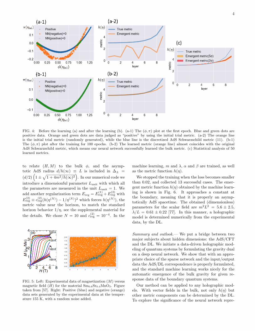
implement our network [74]. The initial metric is ran-domly chosen. Choosing the batch size equal to 10, wefind that after 100 epochs of the training our deep neuralnetwork successfully learned h(η) and it coincides with(11), see Fig. 4 (b) [75]. The statistical analysis with50 learned metric, Fig. 4 (c), shows that the asymptoticAdS region is almost perfectly learned. The near horizonregion has ≈ 30% systematic error, and it is expectedalso for the following analysis with experimental data.

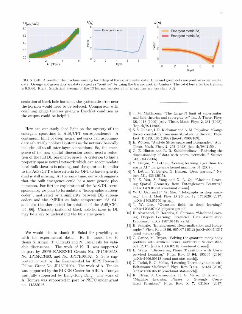
Emergent metric from experiments.— Since we havechecked that the AdS Schwarzschild metric is success-fully reproduced, we shall apply the deep neural net-work to learn a bulk geometry for a given experimen-tal data. We use experimental data of the magnetiza-tion curve (the magnetization M [µB/Mn] vs the externalmagnetic field H [Tesla]) for the 3-dimensional materialSm0.6Sr0.4MnO3 which is known to have a strong quan-tum fluctuation [57], see Fig. 5. We employ a set of dataat temperature 155 K which is slightly above the criticaltemperature, since it exhibits the deviation from a linearM -H curve suggesting a strong correlation. To form apositive data we add a random noise around the experi-mental data, and also generated negative data positionedaway from the positive data.[76]

The same neural network is used, except that we adda new zero-th layer to relate the experimental data with(φ, π), motivated by (9) :

φ(ηini) = αH + βMπ(ηini) = −∆−αH −∆+βM.

(12)

We introduce the normalization parameters α and β

4

FIG. 4: Before the learning (a) and after the learning (b). (a-1) The (φ, π) plot at the first epoch. Blue and green dots arepositive data. Orange and green dots are data judged as “positive” by using the initial trial metric. (a-2) The orange lineis the initial trial metric (randomly generated), while the blue line is the discretized AdS Schwarzschild metric (11). (b-1)The (φ, π) plot after the training for 100 epochs. (b-2) The learned metric (orange line) almost coincides with the originalAdS Schwarzschild metric, which means our neural network successfully learned the bulk metric. (c) Statistical analysis of 50learned metrics.

to relate (H,M) to the bulk φ, and the asymp-totic AdS radius d/h(∞) ≡ L is included in ∆± =

(d/2)(

1±√

1 + 4m2/h(∞)2)

. In our numerical code we

introduce a dimensionful parameter Lunit with which allthe parameters are measured in the unit Lunit = 1. We

add another regularization term Ereg = E(1)reg +E

(2)reg with

E(2)reg ≡ c(2)

reg(h(η(N))− 1/η(N))2 which forces h(η(N)), themetric value near the horizon, to match the standardhorizon behavior 1/η, see the supplemental material for

the details. We chose N = 10 and c(2)reg = 10−4. In the

0 1 2 3 4 5 6

0.00

0.25

0.50

0.75

1.00

1.25

1.50

1.75

2.00

FIG. 5: Left: Experimental data of magnetization (M) versusmagnetic field (H) for the material Sm0.6Sr0.4MnO3. Figuretaken from [57]. Right: Positive (blue) and negative (orange)data sets generated by the experimental data at the temper-ature 155 K, with a random noise added.

machine learning, m and λ, α and β are trained, as wellas the metric function h(η).

We stopped the training when the loss becomes smallerthan 0.02, and collected 13 successful cases. The emer-gent metric function h(η) obtained by the machine learn-ing is shown in Fig. 6. It approaches a constant atthe boundary, meaning that it is properly an asymp-totically AdS spacetime. The obtained (dimensionless)parameters for the scalar field are m2L2 = 5.6 ± 2.5,λ/L = 0.61 ± 0.22 [77]. In this manner, a holographicmodel is determined numerically from the experimentaldata, by the DL.

Summary and outlook.— We put a bridge between twomajor subjects about hidden dimensions: the AdS/CFTand the DL. We initiate a data-driven holographic mod-eling of quantum systems by formulating the gravity dualon a deep neural network. We show that with an appro-priate choice of the sparse network and the input/outputdata the AdS/DL correspondence is properly formulated,and the standard machine learning works nicely for theautomatic emergence of the bulk gravity for given re-sponse data of the boundary quantum systems.

Our method can be applied to any holographic mod-els. With vector fields in the bulk, not only h(η) butother metric components can be determined by the DL.To explore the significance of the neural network repre-

5

FIG. 6: Left: A result of the machine learning for fitting of the experimental data. Blue and green dots are positive experimentaldata. Orange and green dots are data judged as “positive” by using the learned metric (Center). The total loss after the trainingis 0.0096. Right: Statistical average of the 13 learned metrics all of whose loss are less than 0.02.

sentation of black hole horizons, the systematic error nearthe horizon would need to be reduced. Comparison withconfining gauge theories giving a Dirichlet condition asthe output could be helpful.

How can our study shed light on the mystery of theemergent spacetime in AdS/CFT correspondence? Acontinuum limit of deep neural networks can accommo-date arbitrarily nonlocal systems as the network basicallyincludes all-to-all inter-layer connections. So, the emer-gence of the new spatial dimension would need a reduc-tion of the full DL parameter space. A criterion to find aproperly sparse neural network which can accommodatelocal bulk theories is missing, and the question is similarto the AdS/CFT where criteria for QFT to have a gravitydual is still missing. At the same time, our work suggeststhat the bulk emergence could be a more generic phe-nomenon. For further exploration of the AdS/DL corre-spondence, we plan to formulate a “holographic autoen-coder”, motivated by a similarity between DL autoen-coders and the cMERA at finite temperature [63, 64],and also the thermofield formulation of the AdS/CFT[65, 66]. Characterization of black hole horizons in DLmay be a key to understand the bulk emergence.

We would like to thank H. Sakai for providing uswith the experimental data. K. H. would like tothank S. Amari, T. Ohtsuki and N. Tanahashi for valu-able discussions. The work of K. H. was supportedin part by JSPS KAKENHI Grants No. JP15H03658,No. JP15K13483, and No. JP17H06462. S. S. is sup-ported in part by the Grant-in-Aid for JSPS ResearchFellow, Grant No. JP16J01004. The work of A. Tanakawas supported by the RIKEN Center for AIP. A. Tomiyawas fully supported by Heng-Tong Ding. The work ofA. Toimya was supported in part by NSFC under grantno. 11535012.

[1] J. M. Maldacena, “The Large N limit of superconfor-mal field theories and supergravity,” Int. J. Theor. Phys.38, 1113 (1999) [Adv. Theor. Math. Phys. 2, 231 (1998)][hep-th/9711200].

[2] S. S. Gubser, I. R. Klebanov and A. M. Polyakov, “Gaugetheory correlators from noncritical string theory,” Phys.Lett. B 428, 105 (1998) [hep-th/9802109].

[3] E. Witten, “Anti-de Sitter space and holography,” Adv.Theor. Math. Phys. 2, 253 (1998) [hep-th/9802150].

[4] G. E. Hinton and R. R. Salakhutdinov, “Reducing thedimensionality of data with neural networks.,” Science313, 504 (2006).

[5] Y. Bengio, Y. LeCun, “Scaling learning algorithms to-wards AI,” Large-scale kernel machines 34 (2007).

[6] Y. LeCun, Y. Bengio, G. Hinton, “Deep learning,” Na-ture 521, 436 (2015).

[7] Y. Z. You, Z. Yang and X. L. Qi, “Machine Learn-ing Spatial Geometry from Entanglement Features,”arXiv:1709.01223 [cond-mat.dis-nn].

[8] W. C. Gan and F. W. Shu, “Holography as deep learn-ing,” Int. J. Mod. Phys. D 26, no. 12, 1743020 (2017)[arXiv:1705.05750 [gr-qc]].

[9] J. W. Lee, “Quantum fields as deep learning,”arXiv:1708.07408 [physics.gen-ph].

[10] H. Abarbanel, P. Rozdeba, S. Shirman, “Machine Learn-ing, Deepest Learning: Statistical Data AssimilationProblems,” arXiv:1707.01415 [cs.AI].

[11] B. Swingle, “Entanglement Renormalization and Holog-raphy,” Phys. Rev. D 86, 065007 (2012) [arXiv:0905.1317[cond-mat.str-el]].

[12] G. Carleo, M. Troyer, “Solving the quantum many-bodyproblem with artificial neural networks,” Science 355,602 (2017) [arXiv:1606.02318 [cond-mat.dis-nn]].

[13] L. Wang, “Discovering Phase Transitions with Unsu-pervised Learning,” Phys. Rev. B 94, 195105 (2016)[arXiv:1606.00318 [cond-mat.stat-mech]].

[14] G. Torlai, R. G. Melko, “Learning Thermodynamics withBoltzmann Machines,” Phys. Rev. B 94, 165134 (2016)[arXiv:1606.02718 [cond-mat.stat-mech]].

[15] K. Ch’ng, J. Carrasquilla, R. G. Melko, E. Khatami,“Machine Learning Phases of Strongly Corre-lated Fermions,” Phys. Rev. X 7, 031038 (2017)

6

[arXiv:1609.02552 [cond-mat.str-el]].[16] D.-L. Deng, X. Li, S. Das Sarma, “Machine Learning

Topological States,” Phys. Rev. B 96, 195145 (2017)[arXiv:1609.09060 [cond-mat.dis-nn]].

[17] A. Tanaka, A. Tomiya, “Detection of phase transitionvia convolutional neural network,” J. Phys. Soc. Jpn. 86,063001 (2017) [arXiv:1609.09087 [cond-mat.dis-nn]].

[18] T. Ohtsuki, T. Ohtsuki “Deep Learning the QuantumPhase Transitions in Random Two-Dimensional Elec-tron Systems,” J. Phys. Soc. Jpn. 85, 123706 (2016)[arXiv:1610.00462 [cond-mat.dis-nn]].

[19] G. Torlai, R. G. Melko, “A Neural Decoder for Topo-logical Codes,” Phys. Rev. Lett. 119, 030501 (2017)[arXiv:1610.04238 [quant-ph]].

[20] Y. Zhang, E.-A. Kim, “Quantum Loop Topography forMachine Learning,” Phys. Rev. Lett. 118, 216401 (2017)[arXiv:1611.01518 [cond-mat.str-el]].

[21] L.-G. Pang, K. Zhou, N. Su, H. Petersen, H. Stocker,X.-N. Wang, “An equation-of-state-meter of QCD tran-sition from deep learning,” Nature Communications 9,210 (2018) [arXiv:1612.04262 [hep-ph]].

[22] T. Ohtsuki, T. Ohtsuki “Deep Learning the QuantumPhase Transitions in Random Electron Systems: Appli-cations to Three Dimensions,” J. Phys. Soc. Jpn. 86,044708 (2017) [arXiv:1612.04909 [cond-mat.dis-nn]].

[23] J. Chen, S. Cheng, H. Xie, L. Wang, T. Xiang, “On theEquivalence of Restricted Boltzmann Machines and Ten-sor Network States,” arXiv:1701.04831 [cond-mat.str-el].

[24] D.-L. Deng, X. Li, S. Das Sarma, “Quantum Entangle-ment in Neural Network States,” Phys. Rev. X 7, 021021(2017) [arXiv:1701.04844 [cond-mat.dis-nn]].

[25] X. Gao, L.-M. Duan, “Efficient Representation of Quan-tum Many-body States with Deep Neural Networks,”arXiv:1701.05039 [cond-mat.dis-nn].

[26] Y. Huang, J. E. Moore, “Neural network representationof tensor network and chiral states,” arXiv:1701.06246[cond-mat.dis-nn]

[27] K. Mills, M. Spanner, I. Tamblyn, “Deep learning and theSchrodinger equation,” Phys. Rev. A 96, 042113 (2017)[arXiv:1702.01361 [cond-mat.mtrl-sci]].

[28] S. J. Wetzel, “Unsupervised learning of phase tran-sitions: from principal component analysis to varia-tional autoencoders,” Phys. Rev. E 96, 022140 (2017)[arXiv:1703.02435 [cond-mat.stat-mech]].

[29] W. Hu, R. R. P. Singh, R. T. Scalettar, “DiscoveringPhases, Phase Transitions and Crossovers through Un-supervised Machine Learning: A critical examination,”Phys. Rev. E 95, 062122 (2017) [arXiv:1704.00080 [cond-mat.stat-mech]].

[30] F. Schindler, N. Regnault, T. Neupert, “Probing many-body localization with neural networks,” Phys. Rev. B95, 245134 (2017) [arXiv:1704.01578 [cond-mat.dis-nn]].

[31] P. Ponte, R. G. Melko, “Kernel methods for interpretablemachine learning of order parameters,” Phys. Rev. B 96,205146 (2017) [arXiv:1704.05848 [cond-mat.stat-mech]].

[32] M. Koch-Janusz, Z. Ringel, “Mutual Information,Neural Networks and the Renormalization Group,”arXiv:1704.06279 [cond-mat.dis-nn].

[33] Y. Zhang, R. G. Melko, E.-A. Kim, “Machine Learn-ing Z2 Quantum Spin Liquids with Quasi-particle Statis-tics,” Phys. Rev. B 96, 245119 (2017) [arXiv:1705.01947[cond-mat.str-el]].

[34] H. Fujita, Y. O. Nakagawa, S. Sugiura, M. Oshikawa,“Construction of Hamiltonians by machine learning of

energy and entanglement spectra,” arXiv:1705.05372[cond-mat.str-el].

[35] S. J. Wetzel, M. Scherzer, “Machine Learning of ExplicitOrder Parameters: From the Ising Model to SU(2) Lat-tice Gauge Theory,” Phys. Rev. B 96, 184410 (2017)[arXiv:1705.05582 [cond-mat.stat-mech]].

[36] K. Mills, I. Tamblyn, “Deep neural networks for direct,featureless learning through observation: the case of 2dspin models,” arXiv:1706.09779 [cond-mat.mtrl-sci].

[37] H. Saito, “Solving the Bose-Hubbard model with ma-chine learning,” J. Phys. Soc. Jpn. 86, 093001 (2017)[arXiv:1707.09723 [cond-mat.dis-nn]].

[38] N. C. Costa, W. Hu, Z. J. Bai, R. T. Scalettar,R. R. P. Singh, “Learning Fermionic Critical Points,”Phys. Rev. B 96, 195138 (2017) [arXiv:1708.04762 [cond-mat.str-el]].

[39] T. Mano, T. Ohtsuki, “Phase Diagrams of Three-Dimensional Anderson and Quantum Percolation Mod-els using Deep Three-Dimensional Convolutional Neu-ral Network,” J. Phys. Soc. Jpn. 86, 113704 (2017)[arXiv:1709.00812 [cond-mat.dis-nn]].

[40] H. Saito, M. Kato, “Machine learning technique tofind quantum many-body ground states of bosons ona lattice,” J. Phys. Soc. Jpn. 87, 014001 (2018)[arXiv:1709.05468 [cond-mat.dis-nn]].

[41] I. Glasser, N. Pancotti, M. August, I. D. Ro-driguez, J. I. Cirac, “Neural Networks QuantumStates, String-Bond States and chiral topological states,”arXiv:1710.04045 [quant-ph].

[42] R. Kaubruegger, L. Pastori, J. C. Budich, “ChiralTopological Phases from Artificial Neural Networks,”arXiv:1710.04713 [cond-mat.str-el].

[43] Z. Liu, S. P. Rodrigues, W. Cai, “Simulating the IsingModel with a Deep Convolutional Generative AdversarialNetwork,” arXiv:1710.04987 [cond-mat.dis-nn].

[44] J. Venderley, V. Khemani, E.-A. Kim, “Machine learningout-of-equilibrium phases of matter,” arXiv:1711.00020[cond-mat.dis-nn].

[45] Z. Li, M. Luo, X. Wan, “Extracting Critical Exponentby Finite-Size Scaling with Convolutional Neural Net-works,” arXiv:1711.04252 [cond-mat.dis-nn].

[46] E. van Nieuwenburg, E. Bairey, G. Refael, “Learn-ing phase transitions from dynamics,” arXiv:1712.00450[cond-mat.dis-nn].

[47] X. Liang, S. Liu, Y. Li, Y.-S. Zhang. “Generation of Bose-Einstein Condensates’ Ground State Through MachineLearning,” arXiv:1712.10093 [quant-ph].

[48] Y. H. He, “Deep-Learning the Landscape,”arXiv:1706.02714 [hep-th].

[49] Y. H. He, “Machine-learning the string landscape,” Phys.Lett. B 774, 564 (2017).

[50] J. Liu, “Artificial Neural Network in Cosmic Landscape,”arXiv:1707.02800 [hep-th].

[51] J. Carifio, J. Halverson, D. Krioukov and B. D. Nel-son, “Machine Learning in the String Landscape,” JHEP1709, 157 (2017) [arXiv:1707.00655 [hep-th]].

[52] F. Ruehle, “Evolving neural networks with genetic algo-rithms to study the String Landscape,” JHEP 1708, 038(2017) [arXiv:1706.07024 [hep-th]].

[53] A. E. Faraggi, J. Rizos and H. Sonmez, “Classification ofStandard-like Heterotic-String Vacua,” arXiv:1709.08229[hep-th].

[54] J. Carifio, W. J. Cunningham, J. Halverson, D. Kri-oukov, C. Long and B. D. Nelson, “Vacuum Selection

7

from Cosmology on Networks of String Geometries,”arXiv:1711.06685 [hep-th].

[55] I. R. Klebanov and E. Witten, “AdS / CFT correspon-dence and symmetry breaking,” Nucl. Phys. B 556, 89(1999) [hep-th/9905104].

[56] G. T. Horowitz, “Introduction to Holographic Su-perconductors,” Lect. Notes Phys. 828, 313 (2011)[arXiv:1002.1722 [hep-th]].

[57] H. Sakai, Y. Taguchi, Y. Tokura, “Impact of BicriticalFluctuation on Magnetocaloric Phenomena in PerovskiteManganites,” J. Phys. Soc. Japan 78, 113708 (2009).

[58] S. de Haro, S. N. Solodukhin and K. Skenderis, “Holo-graphic reconstruction of space-time and renormalizationin the AdS / CFT correspondence,” Commun. Math.Phys. 217, 595 (2001) [hep-th/0002230].

[59] K. Skenderis, “Lecture notes on holographic renormal-ization,” Class. Quant. Grav. 19, 5849 (2002) [hep-th/0209067].

[60] I. Papadimitriou and K. Skenderis, “AdS / CFT cor-respondence and geometry,” IRMA Lect. Math. Theor.Phys. 8, 73 (2005) [hep-th/0404176].

[61] I. Papadimitriou and K. Skenderis, “Correlation func-tions in holographic RG flows,” JHEP 0410, 075 (2004)[hep-th/0407071].

[62] I. Papadimitriou, “Holographic renormalization as acanonical transformation,” JHEP 1011, 014 (2010)[arXiv:1007.4592 [hep-th]].

[63] H. Matsueda, M. Ishihara and Y. Hashizume, “Tensornetwork and a black hole,” Phys. Rev. D 87, no. 6,066002 (2013) [arXiv:1208.0206 [hep-th]].

[64] A. Mollabashi, M. Nozaki, S. Ryu and T. Takayanagi,“Holographic Geometry of cMERA for QuantumQuenches and Finite Temperature,” JHEP 1403, 098(2014) [arXiv:1311.6095 [hep-th]].

[65] J. M. Maldacena, “Eternal black holes in anti-de Sitter,”JHEP 0304, 021 (2003) [hep-th/0106112].

[66] T. Hartman and J. Maldacena, “Time Evolution of En-tanglement Entropy from Black Hole Interiors,” JHEP1305, 014 (2013) [arXiv:1303.1080 [hep-th]].

[67] We assume that the system can be described holograph-ically by a classical scalar field in asymptotically AdSspace.

[68] See [8, 9] for related essays. A continuum limit of thedeep layers was studied in a different context [10].

[69] An application of DL or machine learning to quantummany-body problems is a rapidly developing subject. See[12] for one of the initial papers, together with recentpapers [13–47]. For machine learning applied to stringlandscape, see [48–54].

[70] In Bayesian neural networks, regularizations are intro-duced as a prior.

[71] Note that ϕ(x2) in (8) includes x1 so it is not local, op-posed to the standard neural network (1) with local ac-tivation functions. See the supplemental material for animproved expression with local activation functions.

[72] The explicit expression for the loss function is availablefor λ = 0: see the supplemental material.

[73] See the supplemental material for the details about thecoordinate system.

[74] See the supplemental material for the details of the setupand coding, and the effect of the regularization and statis-tics.

[75] At the first epoch, the loss was 0.2349, while after the100th epoch, the loss was 0.0002. We terminated the

learning when the loss did not decrease.[76] Our experimental data does not have an error bar, so we

add the noise.[77] For numerically estimated conformal dimension and its

implications, see the supplemental material.

8

Supplemental Material for “Deep Learning and AdS/CFT”

HAMILTONIAN SYSTEMS REALIZED BY DEEP NEURAL NETWORK

Here we show that a restricted class of Hamiltonian systems can be realized by a deep neural network with a localactivation function.[10] We consider a generic Hamiltonian H(p, q) and its Hamilton equation, and seek for a deepneural network representation (1) representing the time evolution by H(p, q). The time direction is discretized to formthe layers. (For our AdS/CFT examples, the radial evolution corresponds to the time direction of the Hamiltonianwhich we consider here.)

Let us try first the following generic neural network and identify the time translation t→ t+∆t with the inter-layerpropagation,

q(t+ ∆t) = ϕ1(W11q(t) +W12p(t)), p(t+ ∆t) = ϕ2(W12q(t) +W22p(t)). (S.13)

This is successive actions of a linear W transformation and a local ϕ nonlinear transformation. The relevant part of

the network is shown in the left panel of Fig. 7. The units x(n)1 and x

(n)2 are directly identified with the canonical

variables q(t) and p(t), and t = n∆t. We want to represent Hamilton equations to be of the form (S.13). It turns outthat it is impossible except for free Hamiltonians.

In order for (S.13) to be consistent at ∆t = 0, we need to require

W11 = 1 +O(∆t), W22 = 1 +O(∆t), W12 = O(∆t), W21 = O(∆t), ϕ(x) = x+O(∆t). (S.14)

So we put an ansatz

Wij = δij + wij∆t, ϕi(x) = x+ gi(x)∆t, (S.15)

where wij (i, j = 1, 2) are constant parameters and gi(x) (i = 1, 2) are nonlinear functions. Substituting these intothe original (S.13) and taking the limit ∆t→ 0, we obtain

q = w11q + w12p+ g1(q), p = w21q + w22p+ g2(p) . (S.16)

For these equations to be Hamiltonian equations, we need to require a symplectic structure

∂

∂q(w11q + w12p+ g1(q)) +

∂

∂p(w21q + w22p+ g2(p)) = 0. (S.17)

However, this equation does not allow any nonlinear activation function gi(x). So, we conclude that a simple identifi-cation of the units of the neural network with the canonical variables allow only linear Hamilton equations, thus freeHamiltonians.

In order for a deep neural network representation to allow generic nonlinear Hamilton equations, we need to improveour identification of the units with the canonical variables, and also of the layer propagation with the time translation.Let us instead try

xi(t+ ∆t) = Wijϕj(Wjkxk(t)). (S.18)

The difference from (S.13) is two folds: First, we define i, j, k = 0, 1, 2, 3 with x1 = q and x2 = p, meaning that we

have additional units x0 and x3. Second, we consider a multiplication by a linear W . So, in total, this is successiveactions of a linear W , a nonlinear local ϕ and a linear W , and we interpret this set as a time translation ∆t. Sincewe pile up these sets as many layers, the last W at t and the next W at t + ∆t are combined into a single lineartransformation Wt+∆tWt, so the standard form (1) of the deep neural network is kept.

We arrange the following sparse weights and local activation functions

W =

0 0 v 00 1 + w11∆t w12∆t 00 w21∆t 1 + w22∆t 00 u 0 0

, W =

0 0 0 0λ1 1 0 00 0 1 λ2

0 0 0 0

,

ϕ0(x0)ϕ1(x1)ϕ2(x2)ϕ3(x3)

=

f(x0)∆t

11

g(x3)∆t

, (S.19)

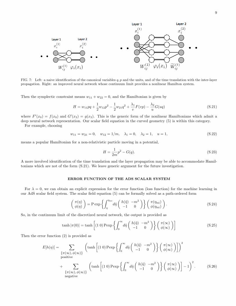
where u, v, wij (i, j = 1, 2) are constant weights, and ϕi(xi) are local activation functions. The network is shown inthe right panel of Fig. 7. Using this definition of the time translation, we arrive at

q = w11q + w12p+ λ1f(vp), p = w11q + w12p+ λ2g(uq). (S.20)

9

FIG. 7: Left: a naive identification of the canonical variables q, p and the units, and of the time translation with the inter-layerpropagation. Right: an improved neural network whose continuum limit provides a nonlinear Hamilton system.

Then the symplectic constraint means w11 + w22 = 0, and the Hamiltonian is given by

H = w11pq +1

2w12p

2 − 1

2w21q

2 +λ1

vF (vp)− λ2

uG(uq) (S.21)

where F ′(x0) = f(x0) and G′(x3) = g(x3). This is the generic form of the nonlinear Hamiltonians which admit adeep neural network representation. Our scalar field equation in the curved geometry (5) is within this category.

For example, choosing

w11 = w21 = 0, w12 = 1/m, λ1 = 0, λ2 = 1, u = 1, (S.22)

means a popular Hamiltonian for a non-relativistic particle moving in a potential,

H =1

2mp2 −G(q). (S.23)

A more involved identification of the time translation and the layer propagation may be able to accommodate Hamil-tonians which are not of the form (S.21). We leave generic argument for the future investigation.

ERROR FUNCTION OF THE ADS SCALAR SYSTEM

For λ = 0, we can obtain an explicit expression for the error function (loss function) for the machine learning inour AdS scalar field system. The scalar field equation (5) can be formally solved as a path-ordered form(

π(η)φ(η)

)= P exp

{∫ ηini

η

dη

(h(η) −m2

−1 0

)}(π(ηini)φ(ηini)

). (S.24)

So, in the continuum limit of the discretized neural network, the output is provided as

tanh |π(0)| = tanh

[(1 0) Pexp

{∫ ∞0

dη

(h(η) −m2

−1 0

)}(π(∞)φ(∞)

)](S.25)

Then the error function (2) is provided as

E[h(η)] =∑

{π(∞), φ(∞)}positive

(tanh

[(1 0) Pexp

{∫ ∞0

dη

(h(η) −m2

−1 0

)}(π(∞)φ(∞)

)])2

+∑

{π(∞), φ(∞)}negative

(tanh

[(1 0) Pexp

{∫ ∞0

dη

(h(η) −m2

−1 0

)}(π(∞)φ(∞)

)]− 1

)2

. (S.26)

10

The learning process is equivalent to the following gradient flow equation with a fictitious time variable τ ,

∂h(η, τ)

∂τ=∂E[h(η, τ)]

∂h(η, τ). (S.27)

For the training of our numerical experiment using the experimental data, we have chosen the initial configurationof h(η) as a constant (which corresponds to a pure AdS metric). For a constant h(η) = h, the error function can beexplicitly evaluated with

π(0) =1

λ+ − λ−(λ+(π(ηini)− λ−φ(ηini))e

−λ+ηini + λ−(−π(ηini) + λ+φ(ηini))e−λ−ηini

)(S.28)

where λ± ≡ 12 (−h ±

√h2 + 4m2) is the eigenvalue of the matrix which is path-ordered. Using this expression, we

find that at the initial epoch of the training the function h(η) is updated by an addition of a function of the formexp[(λ+ − λ−)η] and of the form exp[−(λ+ − λ−)η]. This means that the update is effective in two regions: near theblack hole horizon η ≈ 0 and near the AdS boundary η ≈ ∞.

Normally in deep learning the update is effective near the output layer because any back propagation could besuppressed by the factor of the activation function. However our example above shows that the update near the inputlayer is also updated. The reason for this difference is that in the example above we assumed λ = 0 to solve the errorfunction explicitly, and it means that the activation function is trivial. In our numerical simulations where λ 6= 0, theback propagation is expected to be suppressed near the input layer.

BLACK HOLE METRIC AND COORDINATE SYSTEMS

Here we summarize the properties of the bulk metric and the coordinate frame which we prefer to use in the maintext.

The 4-dimensional AdS Schwarzschild black hole metric is given by

ds2 = −f(r)dt2 +1

f(r)dr2 +

r2

L2

2∑i=1

dx2i , f(r) ≡ r2

L2

(1− r3

0

r3

)(S.29)

where L is the AdS radius, and r = r0 is the location of the black hole horizon. r = ∞ corresponds to the AdSboundary. To bring it to the form (4), we make a coordinate transformation

r = r0

(cosh

3η

2L

)2/3

. (S.30)

With this coordinate η, the metric is given by

ds2 = −f(η)dt2 + dη2 + g(η)

2∑i=1

dx2i , f(η) ≡ r2

0

L2

(cosh

3η

2L

)−2/3(sinh

3η

2L

)2

, g(η) ≡ r20

L2

(cosh

3η

2L

)4/3

. (S.31)

The AdS boundary is located at η = ∞ while the black hole horizon resides at η = 0. The function h(η) appearingin the scalar field equation (5) is

h(η) ≡ ∂η log√f(η)g(η)d−1 =

3

Lcoth

3η

L. (S.32)

The r0 dependence, and hence the temperature dependence, disappears because our scalar field equation (5) assumestime independence and xi-independence. This h(η) is basically the invariant volume of the spacetime, and is importantin the sense that a certain tensor component of the vacuum Einstein equation coming from

SE =

∫d4x√−det g

(R+

6

L2

)(S.33)

results in a closed form

− 9

L2+ ∂ηh(η) + h(η)2 = 0 . (S.34)

11

It can be shown that the ansatz (S.29) leads to a unique metric solution for the vacuum Einstein equations, and thesolution is given by (S.32) up to a constant shift of η. Generically, whatever the temperature is, and whatever thematter energy momentum tensor is, the metric function h(η) behaves as h(η) ≈ 1/η near the horizon η ≈ 0, and goesto a constant (proportional to the AdS radius L) at the AdS boundary η ≈ ∞.

One may try to impose some physical condition on h(η). In fact, the right hand side of (S.34) is a linear combinationof the energy momentum tensor, and generally we expect that the energy momentum tensor is subject to variousenergy conditions, which may constrain the η-evolution of h(η). Unfortunately it turns out that a suitable energycondition for constraining h(η) is not available, within our search. So, non-monotonic functions in η are allowed as alearned metric.

DETAILS ABOUT OUR CODING FOR THE LEARNING

Comments on the regularization

Before getting into the detailed presentation of the coding, let us make some comments on the effect of the regu-larization Ereg and the statistical analysis of the learning trials.

First, we discuss the meaning of Ereg in (2). In the first numerical experiment for the reproduction of the AdSSchwarzschild black hole metric we took

E(1)reg ≡ 3× 10−3

N−1∑n=1

(η(n))4(h(η(n+1))− h(η(n))

)2

∝∫dη (h′(η)η2)2. (S.35)

This regularization term works as a selection of the metrics which are smooth. We are interested in the metric withwhich we can take a continuum limit, so a smooth h(η) is better for our physical interpretation. Without Ereg, thelearned metrics are far from the AdS Schwarzschild metric: see Fig.8 for an example of the learned metric withoutEreg. Note that the example in Fig. 8 achieves the accuracy which is the same order as that of the learned metricwith Ereg. So, in effect, this regularization term does not spoil the learning process, but actually picks up the metricswhich are smooth, among the learned metrics achieving the same accuracy.

Second, we discuss how the learned metric shown in Fig. 4 is generic, for the case of the first numerical experiment.We have collected results of 50 trials of the machine learning, and the statistical analysis is presented in Fig. 4 (c). Itis shown that the metric in the asymptotic region is quite nicely learned, and we can conclude that the asymptoticAdS spacetime has been learned properly. On the other hand, for the result in the region near the black hole horizon,the learned metric reproduces qualitatively the behavior around the horizon, but quantitatively it deviates from thetrue metric. This could be due to the discretization of the spacetime.

Third, let us discuss the regularization for the second numerical experiment for the emergence of the metric for thecondensed mater material data. The regularization used is

Ereg = E(1)reg + E(2)

reg

= 3× 10−3N−1∑n=1

(η(n))4(h(η(n+1))− h(η(n))

)2

+ c(2)reg

(h(η(N))− 1/η(N)

)2

, (S.36)

with c(2)reg = 10−4. The second term is to fit the metric h(η) near the horizon to the value 1/η, because 1/η behavior is

expected for any regular horizons. In Fig. 9, we present our statistical analyses of the obtained metrics for two other

distinct choices of the regularization parameter: c(2)reg = 0 and c

(2)reg = 0.1. For c

(2)reg = 0, there is no regularization Ereg,

so the metric goes down to a negative number at the horizon. For c(2)reg = 0, which is a strong regularization, the metric

is almost completely fixed to a value 1/η with η = η(N). For all cases, the learned metrics achieve a loss ≈ 0.02, sothe system is successfully learned. The only difference is how we pick up ”physically sensible” metrics among many

learned metrics. In Fig. 6, we chose c(2)reg = 10−4 which is in between the values used in Fig. 9, because the deviation

of the metric near the horizon is of the same order as that near the asymptotic region.

Numerical experiment 1: Reconstructing AdS Schwarzschild black hole

We have performed two independent numerical experiments: The first one is about the reconstruction of the AdSSchwarzschild black hole metric, and the second one is about the emergence of a metric from the experimental data of

12

FIG. 8: A learned metric with a high accuracy, without the use of the regularization Ereg. The used setup is the same aswhat we used for the reproduction of the AdS Schwarzschild metric.

FIG. 9: Statistical results of the obtained 13 metrics. Left: c(2)reg = 0. Right: c

(2)reg = 0.1.

a condensed matter material. Here we explain details about the coding and the setup, for each numerical experiment.In the first numerical experiment, we fix the mass of the scalar field m2 and coupling constant in potential V (φ) =

λ4φ

4 to

m2 = −1, λ = 1, (S.37)

and prepare data {(x(1), y)} to train the neural network. The training data is just a list of initial pairs of x(1) = (φ, π)and corresponding answer signal y. We regard x(1) = (φ, π) as field values at the AdS boundary, and define the answersignal so that it represents whether they are permissible or not when they propagate toward the black hole horizon.More explicitly, what we do is the iteration defined below:

1. randomly choose φ ∈ [0, 1.5], π ∈ [−0.2, 0.2] and regard them as input : x(1) =

(φπ

).

2. propagate it by E.O.M (6) with AdS Schwarzschild metric (11) from

(φ(ηini) = φπ(ηini) = π

)to

(φ(ηfin)π(ηfin)

).

3. calculate consistency F , i.e. right hand side of (10), and define the answer signal : y =

{0 if F < 0.11 if F > 0.1

.

To train the network appropriately, it is better to prepare a data containing roughly equal number of y = 0 samplesand y = 1 samples. We take a naive strategy here: If the result of step 3 becomes y = 0, we add the sample (x(1), y)to the positive data category, if not, we add the sample to the negative data category. Once the number of samples

13

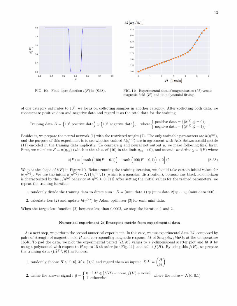
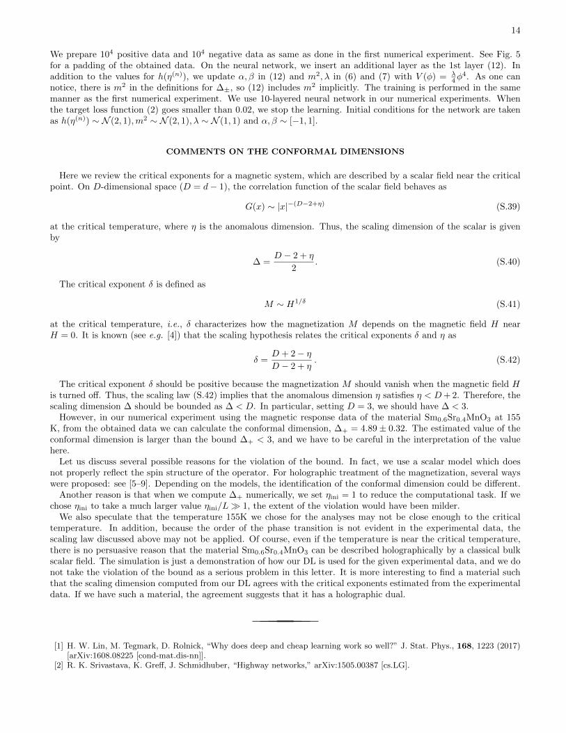
FIG. 10: Final layer function t(F ) in (S.38). FIG. 11: Experimental data of magnetization (M) versusmagnetic field (H) and its polynomial fitting.

of one category saturates to 103, we focus on collecting samples in another category. After collecting both data, weconcatenate positive data and negative data and regard it as the total data for the training:

Training data D =(

103 positive data)⊕(

103 negative data), where

{positive data = {(x(1), y = 0)}negatve data = {(x(1), y = 1)} .

Besides it, we prepare the neural network (1) with the restricted weight (7). The only trainable parameters are h(η(n)),and the purpose of this experiment is to see whether trained h(η(n)) are in agreement with AdS Schwarzschild metric(11) encoded in the training data implicitly. To compare y and neural net output y, we make following final layer.First, we calculate F ≡ π(ηfin) (which is the r.h.s. of (10) in the limit ηfin → 0), and second, we define y ≡ t(F ) where

t(F ) =[

tanh(

100(F − 0.1))− tanh

(100(F + 0.1)

)+ 2]/2. (S.38)

We plot the shape of t(F ) in Figure 10. Before running the training iteration, we should take certain initial values forh(η(n)). We use the initial h(η(n)) ∼ N (1/η(n), 1) (which is a gaussian distribution), because any black hole horizonis characterized by the 1/η(n) behavior at η(n) ≈ 0. [11] After setting the initial values for the trained parameters, werepeat the training iteration:

1. randomly divide the training data to direct sum : D = (mini data 1)⊕ (mini data 2)⊕ · · · ⊕ (mini data 200).

2. calculate loss (2) and update h(η(n)) by Adam optimizer [3] for each mini data.

When the target loss function (2) becomes less than 0.0002, we stop the iteration 1 and 2.

Numerical experiment 2: Emergent metric from experimental data

As a next step, we perform the second numerical experiment. In this case, we use experimental data [57] composed bypairs of strength of magnetic field H and corresponding magnetic response M of Sm0.6Sr0.4MnO3 at the temperature155K. To pad the data, we plot the experimental paired (H,M) values to a 2-dimensional scatter plot and fit it byusing a polynomial with respect to H up to 15-th order (see Fig. 11), and call it f(H). By using this f(H), we preparethe training data {(X(1), y)} as follows:

1. randomly choose H ∈ [0, 6],M ∈ [0, 2] and regard them as input : X(1) =

(HM

)

2. define the answer signal : y =

{0 if M ∈ [f(H)− noise, f(H) + noise]1 otherwise

where the noise ∼ N (0, 0.1)

14

We prepare 104 positive data and 104 negative data as same as done in the first numerical experiment. See Fig. 5for a padding of the obtained data. On the neural network, we insert an additional layer as the 1st layer (12). Inaddition to the values for h(η(n)), we update α, β in (12) and m2, λ in (6) and (7) with V (φ) = λ

4φ4. As one can

notice, there is m2 in the definitions for ∆±, so (12) includes m2 implicitly. The training is performed in the samemanner as the first numerical experiment. We use 10-layered neural network in our numerical experiments. Whenthe target loss function (2) goes smaller than 0.02, we stop the learning. Initial conditions for the network are takenas h(η(n)) ∼ N (2, 1),m2 ∼ N (2, 1), λ ∼ N (1, 1) and α, β ∼ [−1, 1].

COMMENTS ON THE CONFORMAL DIMENSIONS

Here we review the critical exponents for a magnetic system, which are described by a scalar field near the criticalpoint. On D-dimensional space (D = d− 1), the correlation function of the scalar field behaves as

G(x) ∼ |x|−(D−2+η) (S.39)

at the critical temperature, where η is the anomalous dimension. Thus, the scaling dimension of the scalar is givenby

∆ =D − 2 + η

2. (S.40)

The critical exponent δ is defined as

M ∼ H1/δ (S.41)

at the critical temperature, i.e., δ characterizes how the magnetization M depends on the magnetic field H nearH = 0. It is known (see e.g. [4]) that the scaling hypothesis relates the critical exponents δ and η as

δ =D + 2− ηD − 2 + η

. (S.42)

The critical exponent δ should be positive because the magnetization M should vanish when the magnetic field His turned off. Thus, the scaling law (S.42) implies that the anomalous dimension η satisfies η < D+ 2. Therefore, thescaling dimension ∆ should be bounded as ∆ < D. In particular, setting D = 3, we should have ∆ < 3.

However, in our numerical experiment using the magnetic response data of the material Sm0.6Sr0.4MnO3 at 155K, from the obtained data we can calculate the conformal dimension, ∆+ = 4.89± 0.32. The estimated value of theconformal dimension is larger than the bound ∆+ < 3, and we have to be careful in the interpretation of the valuehere.

Let us discuss several possible reasons for the violation of the bound. In fact, we use a scalar model which doesnot properly reflect the spin structure of the operator. For holographic treatment of the magnetization, several wayswere proposed: see [5–9]. Depending on the models, the identification of the conformal dimension could be different.

Another reason is that when we compute ∆+ numerically, we set ηini = 1 to reduce the computational task. If wechose ηini to take a much larger value ηini/L� 1, the extent of the violation would have been milder.

We also speculate that the temperature 155K we chose for the analyses may not be close enough to the criticaltemperature. In addition, because the order of the phase transition is not evident in the experimental data, thescaling law discussed above may not be applied. Of course, even if the temperature is near the critical temperature,there is no persuasive reason that the material Sm0.6Sr0.4MnO3 can be described holographically by a classical bulkscalar field. The simulation is just a demonstration of how our DL is used for the given experimental data, and we donot take the violation of the bound as a serious problem in this letter. It is more interesting to find a material suchthat the scaling dimension computed from our DL agrees with the critical exponents estimated from the experimentaldata. If we have such a material, the agreement suggests that it has a holographic dual.

[1] H. W. Lin, M. Tegmark, D. Rolnick, “Why does deep and cheap learning work so well?” J. Stat. Phys., 168, 1223 (2017)[arXiv:1608.08225 [cond-mat.dis-nn]].

[2] R. K. Srivastava, K. Greff, J. Schmidhuber, “Highway networks,” arXiv:1505.00387 [cs.LG].

15

[3] D. Kingma and J. Ba: “Adam: A method for stochastic optimization,” arXiv:1412.6980 [cs.LG].[4] P. Di Francesco, P. Mathieu and D. Senechal, “Conformal Field Theory,”[5] N. Iqbal, H. Liu, M. Mezei and Q. Si, “Quantum phase transitions in holographic models of magnetism and superconduc-

tors,” Phys. Rev. D 82, 045002 (2010) [arXiv:1003.0010 [hep-th]].[6] K. Hashimoto, N. Iizuka and T. Kimura, “Towards Holographic Spintronics,” Phys. Rev. D 91, no. 8, 086003 (2015)

[arXiv:1304.3126 [hep-th]].[7] R. G. Cai and R. Q. Yang, “Paramagnetism-Ferromagnetism Phase Transition in a Dyonic Black Hole,” Phys. Rev. D 90,

no. 8, 081901 (2014) [arXiv:1404.2856 [hep-th]].[8] R. G. Cai, R. Q. Yang, Y. B. Wu and C. Y. Zhang, “Massive 2-form field and holographic ferromagnetic phase transition,”

JHEP 1511, 021 (2015) [arXiv:1507.00546 [hep-th]].[9] N. Yokoi, M. Ishihara, K. Sato and E. Saitoh, “Holographic realization of ferromagnets,” Phys. Rev. D 93, no. 2, 026002

(2016) [arXiv:1508.01626 [hep-th]].[10] Here we regard the time evolution of the Hamiltonian as the propagation in the neural network. For other ways to identify

Hamiltonian systems in machine learning, see [1].[11] Note that we do not teach the value of h(η) at the AdS boundary, i.e. 3 in our case.