Introduction The interplay between local and global ... · Introduction The interplay between local and global ... Our SDSS galaxies have star ... If instead of the considered functional

Introduction The interplay between local and global

processes in galaxies

C. Jakob Walcher Leibniz Institut für Astrophysik Potsdam (AIP)

Introduction Why this is NOT and IFU conference!!

C. Jakob Walcher Leibniz Institut für Astrophysik Potsdam (AIP)

11.4.2016 Cozumel, Walcher

Global M-Z ⬌ local Σ-Z

3

Tremonti et al., 2004mass, we invoke another well-known empirical correlation,the Schmidt star formation law (Schmidt 1959; Kennicutt1998), which relates the star formation surface density to thegas surface density.

For each of our galaxies we calculate the star formation rate(SFR) in the fiber aperture from the attenuation-corrected H!luminosity following Brinchmann et al. (2004).

We multiply our SFRs by a factor of 1.5 to convert from aKroupa (2001) IMF to the Salpeter IMF used by Kennicutt(1998). Our SDSS galaxies have star formation surface den-sities that are within a factor of 10 of !SFR ¼ 0:3 M" yr#1

kpc#2, exactly the range found by Kennicutt (1998) for thecentral regions of normal disk galaxies. We convert star for-mation surface density to surface gas mass density, !gas, byinverting the composite Schmidt law of Kennicutt (1998),

!SFR ¼ 1:6 ; 10#4 !gas

1 M" pc#2

! "1:4

M" yr#1 kpc#2: ð5Þ

(Note that the numerical coefficient has been adjusted to in-clude helium in !gas.) Combining our spectroscopically de-rived M/L ratio with a measurement of the z-band surfacebrightness in the fiber aperture, we compute !star, the stellarsurface mass density. The gas mass fraction is then "gas ¼!gas=(!gas þ !star).

In Figure 8 we plot the effective yield of our SDSS star-forming galaxies as a function of total baryonic (stellar+gas)mass. Baryonic mass is believed to correlate with dark mass, asevidenced by the existence of a baryonic ‘‘Tully-Fisher’’ rela-tion (McGaugh et al. 2000; Bell & de Jong 2001). We are inter-ested in the dark mass because departures from the ‘‘closedbox’’ model might be expected to correlate with the depth ofthe galaxy potential well. Data on the distribution of the ef-fective yield at fixed baryonic mass are provided in Table 4.Because very few of our SDSS galaxies have masses below108.5 M", we augment our data set with measurements fromLee et al. (2003), Garnett (2002), and Pilyugin & Ferrini(2000), all of which use direct gas mass measurements. We

Fig. 6.—Relation between stellar mass, in units of solar masses, and gas-phase oxygen abundance for '53,400 star-forming galaxies in the SDSS. The largeblack filled diamonds represent the median in bins of 0.1 dex in mass that include at least 100 data points. The solid lines are the contours that enclose 68% and 95%of the data. The red line shows a polynomial fit to the data. The inset plot shows the residuals of the fit. Data for the contours are given in Table 3.

ORIGIN OF MASS-METALLICITY RELATION 907No. 2, 2004

Stellar mass

TBW: The Mass-Metallity relation explored with CALIFA:

0 1 2 3 4

88.

59

12+l

og (O

/H) O

3N2

0 1 2 3 4

-3-2

-10

0 1 2 3 4

88.

59

12+l

og (O

/H) O

3N2

-2-1

Δ 1

2+lo

g (O

/H) O

3N2

-3 -2 -1

-0.2

00.

2

10 20

% HII reg.

Fig. 3. . Top-left panel: Distribution of the oxygen abundances for the 3000 individual H ii regions extracted from the CALIFA data, along thesurface mass density, represented with a density contour-plot. The first contour encircles a 95% of the total number of H ii regions. The solid-bluepoints represent the average oxygen abundances, with their corresponding standard deviations indicated as error bars, for consecutive bins of 0.1dex in surface mass density. The solid line represents the best fitted curve for these points. Top-right panel: Distribution of the SFR surface densityalong the stellar mass density each individual H ii region. The contour plots represent the density of points in the distribution of oxygen abundancesalong the surface SFR densities. The first contour encircles a 95% of the total number of H ii regions. Bottom-left panel: Same distribution shownin the top-left panel, for the CALIFA and feasibility-studies objects. The colors represent the logarithm of the integrated surface density of the SFRfor each H ii region. Bottom-right panel: Distribution of the differential oxygen abundance, once the dependency with the surface mass density hasbeen subtracted, for individual H ii regions. The contour plots represent the density of points in the distribution of differential oxygen abundances,ones subtracted the dependence with the surface masses densities, along the surface SFR densities. The first contour encircles a 95% of the totalnumber of H ii regions. The solid-blue points represent the average differential abundances, with their corresponding standard deviations indicatedas error bars, for consecutive bins of 0.1 dex in surface SFR density.

ter parameters governs how metallicity actually increases withmass, while the first one is the asymptotic oxygen abundancefor large masses. This value can be interpreted as the maximummetallicity of the universe at a certain redshift. As shows byMoustakas et al. (2011), this parameter evolves with redshift atabout −0.2∆log(O/H)

∆z . The functional form describe well the con-sidered data, as it can be appreciated in Fig. 2. The dispersionof the abundance values along this curve is σ∆log(O/H) =0.069dex, much smaller than previous reported values by (e.g., T04Mannucci et al. 2010; Hughes et al. 2012, all of them ∼0.1dex). Although the dispersion around the correlation depends onthe actual form adopted for the M-Z relation, the derived valueis alwasy low. If instead of the considered functional form weadopt a 3 or 4 order polynomial function, as the one consideredby Kewley & Ellison (2008), the dispersion is just 0.084 dex,smaller than the value reported in that publication for SDSS datausing the same calibrator. In any case, our adopted functionalform is the one that reduces more the dispersion around the fit-ted value from the different ones that we have tested.

Once derived this functional form, we have determined theoffset and dispersion for the data corresponding to the galaxiesanalyzed in Sánchez et al. (2012). Based also on IFS, and cov-ering the full optical extension of the galaxies, the only possibledifference would be either the detail sample selection and/or theredshift range. The galaxies from the feasibility studies consid-ered here are all of them face-on spiral galaxies, with a sim-ilar average redshift than the CALIFA data (z ∼0.016), andonly slightly larger projected size (red squares in Fig. 2). Theypresent a minor offset with respect to the derived M-Z rela-tion (∆log(O/H) = −0.003 dex) and a slightly larger dispersion(σ∆log(O/H) =0.084 dex). Considering that the spectrophotomet-ric calibration of the data is slight worse (Mármol-Queraltó et al.2011), the slightly larger redshift range covered by this sample(Sánchez et al. 2012), and that the sample is more reduced (31objects), the difference is not significant. If we considered to-gether those data and the CALIFA ones described before, thederived dispersion is quite low (σ∆log(O/H) =0.073).

Finally, for the PINGS data, there is a clear offset with re-spect to the M-Z relation (∆log(O/H) =0.117 dex) and a clear

6

Stellar Mass Surface densitySanchez et al., 2013

[O/H][O/H]


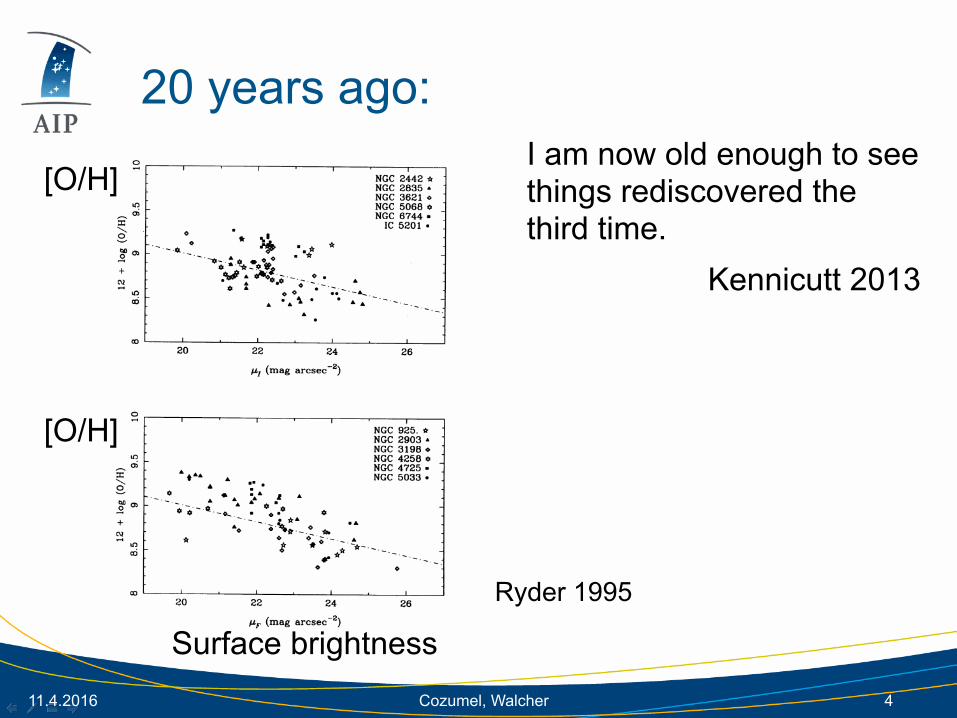
20 years ago:

4

1995ApJ...444..610R

Ryder 1995

Surface brightness

[O/H]

[O/H]I am now old enough to see things rediscovered the third time.

Kennicutt 2013


Local: Escape velocity and abundances

5

ATLAS3D, Scott et al., 2013

MgB

Fe50

15Hβ

Vesc


Global SF MS ⬌ local SF MS

6

Sta

r For

mat

ion

Rat

e

Galaxy MassSanchez et al., 2013, Cano-Diaz, et al., subm. see also Catalan-Torecilla, et al., 2015

A&A 554, A58 (2013)

9 10 11

88.

59

12+l

og(O

/H)

Re

O3N

2

9 10 11

-10

1

9 10 11

88.

59

12+l

og(O

/H)

Re

O3N

2

-0.8

-0.6

-0.4

-0.2

0.0

+0.2

+0.4

+0.6

+0.8

+1.0

-1 0 1

-0.2

00.

2

∆ 12

+log

(O/H

) Re

O3N

2

10 20

% Obj.

Fig. 4. . Top-left panel: distribution of the oxygen abundances at the effective radii as a function of the integrated stellar masses for the CALIFAgalaxies (113, blue solid circles). For comparison purposes, we show similar values for the galaxies observed in the CALIFA feasibility studies (31,red solid squares) included in the H II regions catalog described in Sánchez et al. (2012b). The size of the symbols is proportional to the integratedSFR. The solid line represents the best-fitted curve, as described in the text. We also included the distribution of abundaces as a function of thestellar masses for the SDSS data corresponding to the redshift ranges sampled by Lara-López et al. (2010), dashed black contours, and Mannucciet al. (2010), solid grey contours. In both cases, the first contour encircles the 95% of the objects, and 20% less objects in each consecutivecontour. Top-right panel: distribution of the integrated SFR as a function of the stellar masses. The size of the symbols is proportional to theoxygen abundance shown in previous panel. The solid line represents the best fitted linear regression to the CALIFA data. Like in the previospanel the contours represent the distribution of both parameters corresponding to the redshift ranges sampled by Lara-López et al. (2010), dashedblack contours, and Mannucci et al. (2010), solid grey contours Bottom-left panel: same distribution shown in the top-left panel, for the CALIFAand feasibility-studies objects. The colors represent the logarithm of the integrated SFR for each galaxy. Bottom-right Panel: distribution of thedifferential oxygen abundances at the effective radii, once the dependency with the stellar mass has been subtracted, as a function of the integratedSFR for the CALIFA galaxies (113, blue solid circles). The size of the symbols is proportional to the oxygen abundances shown in Fig. 4. Thehistogram shows the same distribution of differential oxygen abundances. The solid line represents a Gaussian function with the same central value(0.01 dex) and standard deviation (0.07 dex) as the represented distribution, scaled to match the histogram.

oxygen abundances estimated for each galaxy at the effectiveradius using the radial gradients with the oxygen abundancesderived directly from the spectra integrated over the entire field-of-view. As expected, both parameters shows a tight correlation(σ ∼ 0.06 dex). The errors estimated for the integrated abun-dance are larger, and they are directly transferred to the disper-sion along the one-to-one relation, and thus, to the correspondingM-Z distribution.

Once this functional form had been derived, we determinedthe offset and dispersion for the data corresponding to the galax-ies analyzed in Sánchez et al. (2012b). Based also on IFS, andcovering the full optical extent of the galaxies, the only pos-sible differences would be either the details of the sample se-lection and/or the redshift range. The galaxies from the fea-sibility studies considered here are all face-on spiral galaxies,with an average redshift similar to that of the CALIFA data(z ∼ 0.016), and only slightly higher projected sizes (red squares

in Fig. 4). They present a minor offset with respect to the derivedM-Z relation (∆log (O/H) = −0.003 dex) and a slightly broaderdispersion (σ∆log (O/H) = 0.084 dex). Considering that the spec-trophotometric calibration of the data is not that accurate (∼20%,Mármol-Queraltó et al. 2011), the slightly larger redshift rangecovered by this sample (Sánchez et al. 2012b), and consider-ing that the sample is smaller (31 objects), the difference is notsignificant. If we consider this dataset and the CALIFA one de-scribed before, the derived dispersion is just σ∆log (O/H) = 0.07.

3.3. Dependence of theM-Z relation on the SFR

The main goal of this study is to explore whether there is a de-pendence of the M-Z relation on the SFR. Before doing that, itis important to understand the possible additional dependenceof the SFR on other properties of the galaxies, in particularon the stellar mass. The SFR of blue/star-forming galaxies has

A58, page 8 of 19

A&A 554, A58 (2013)

0 1 2 3 4

88.

59

12+

log

(O/H

) O

3N2

0 1 2 3 4

-3-2

-10

0 1 2 3 4

88.

59

12+

log

(O/H

) O

3N2

-2-1

∆ 12

+log

(O/H

) O3N

2

-3 -2 -1

-0.2

00.

2

10 20

% HII reg.

Fig. 5. . Top-left panel: distribution of the oxygen abundances for the 3000 individual H II regions extracted from the CALIFA data as a functionof the surface mass density, represented with a density contour-plot. The first contour encircles 95% of the total number of H II regions, with∼20% less in each consecutive contour. The solid-yellow points represent the average oxygen abundances, with their corresponding standarddeviations indicated as error bars for consecutive bins of 0.1 dex in surface mass density. The dot-dashed line represents the best-fitted curve forthese points. Top-right panel: distribution of the SFR surface density as a function of the stellar mass density of each individual H II region. Thecontour plots represent the density of points in the distribution of oxygen abundances as a function of the surface SFR densities, with the sameencircled numbers as in the previous panel. Bottom-left panel: same distribution shown in the top-left panel, for the CALIFA and feasibility-studiesobjects. The colors represent the logarithm of the integrated surface density of the SFR for each H II region. Bottom-right panel: distribution of thedifferential oxygen abundance, once the dependency with the surface mass density has been subtracted, for individual H II regions. The contourplots represent the density of points in the distribution of differential oxygen abundances, once subtracted the dependence on the surface massesdensities, as a function of the surface SFR densities, with the same encircled numbers as in the previous panel. The solid-yellow points representthe average values for the abundance offsets, with their corresponding standard deviations indicated as error bars, for consecutive bins of 0.1 dexin surface SFR density.

by a simple linear regression. The surface star-formation den-sity scales with the surface mass density with a slope of α =0.66 ± 0.18, again, below the expected value derived in semi-analytical simulations for the mass-SFR relation. Note that acomparison with a simulation taking into account the describedlocal relationship is not feasible at present, since no such simu-lation exists to our knowledge.

This relation indicates that the HII regions with stronger star-formation are located in more massive areas of the galaxies (i.e.,towards the center). We explored if our result is affected byyoung stars that biases our mass derivation. However, we foundthat our surface-brightness and colors (the two parameters usedto derive the masses) are not strongly correlated with either theage of the underlying stellar population or the fraction of youngstars. Even more, the SFR density presents a positive weak trendwith the B − V color, not the other way round.

Like in the global case, these two relations between theoxygen abundance and the surface SFR with the surface massdensity may induce a third relation between the two former

parameters. In fact, there is a trend between the two parame-ters, much weaker than the other two described here (r = 0.59),as expected from an induced correlation. Figure 5 bottom-leftpanel illustrates this dependence, showing the local-M-Z rela-tion, color-coded by the mean surface SFR per bin of oxygenabundance and surface mass density. There is a clear gradientin the surface SFR that mostly follows the local-M-Z relation.In this figure we can see a deviation from this global trendin agreement with the results by Lara-López et al. (2010) andMannucci et al. (2010), in the sense that there are a few H II re-gions with a low metal content and high SFR for their corre-sponding mass surface density (bottom-right edge of the figure).However, all together they represent less than a 2−3% of thetotal sampled regions, and therefore cannot explain a global ef-fect as described in these publications. Furthermore, the stochas-tic fluctuations around the average values at this low numberstatistics may clearly produce this effect, since there are otherH II regions in the same location of the diagram with much lowersurface SFR.

A58, page 10 of 19

Sta

r For

mat

ion

Rat

eStellar Mass Surface Density


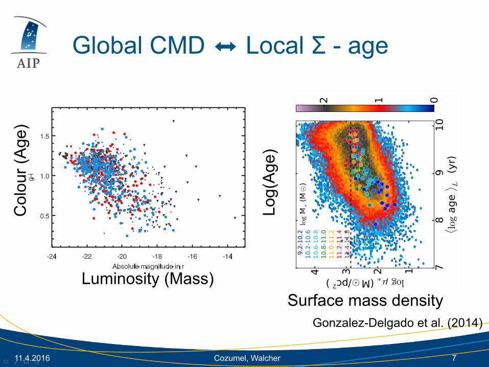
Global CMD ⬌ Local Σ - age

7

Gonzalez-Delgado et al. (2014)

Log(

Age

)

Surface mass density

Col

our (

Age

)

Luminosity (Mass)Th

eC

ALI

FAco

llabo

ratio

n:Th

est

arfo

rmat

ion

hist

ory

ofC

ALI

FAga

laxi

es

Fig.

10.

Rel

atio

nbe

twee

naM 50/a

L 50an

dth

eto

tal

stel

lar

mas

s.Po

ints

are

colo

red

acco

rdin

gto

the

lum

inos

ityw

eigh

ted

age

ofth

est

ella

rpop

ulat

ion

atR=

0.5a

L 50.G

alax

iesw

ithco

ncen

tratio

nin

dex

C�

2.8

are

mar

ked

with

acr

oss.

Das

hed

blue

line

show

the

fitfo

rall

the

gala

xies

with

log

M⇤

(M�)

11,d

ashe

dre

dfo

rlo

gM⇤

(M�)>

11,a

nddo

tted

blue

and

red

lines

are

the

fitfo

rdi

skdo

min

ated

gala

xies

and

sphe

roid

alga

laxi

es,r

espe

ctiv

ely.

colo

rs.T

hey

find

that

ages

are

muc

hbe

tterc

orre

late

dw

ithth

eir

loca

lsu

rfac

ebr

ight

ness

than

with

the

gala

xyab

solu

tem

agni

-tu

dein

the

Kba

nd,a

ndco

nclu

deth

atth

esu

rfac

ede

nsity

play

sa

mor

efu

ndam

enta

lrol

ein

the

SFH

ofdi

sks

than

the

mas

sof

the

gala

xy.T

hey

sugg

est

that

the

corr

elat

ion

can

beex

plai

ned

thro

ugh

ade

pend

ence

ofth

est

arfo

rmat

ion

law

onth

elo

cald

en-

sity

(see

also

Bel

l&B

owen

2000

;Boi

ssie

r&

Pran

tzos

2000

).N

ote

that

they

assu

me

that

colo

rstra

ceag

e,an

dus

esu

rfac

ebr

ight

ness

and

tota

llum

inos

ityas

prox

ies

forµ⇤

and

M⇤

resp

ec-

tivel

y.Fu

rther

mor

e,th

isco

nclu

sion

was

obta

ined

only

fors

pira

lga

laxi

es.

Inth

elig

htof

this

resu

lt,an

dar

med

with

our

spec

-tro

scop

ical

lyde

rived

prop

ertie

s,w

eas

kw

heth

erth

isco

nclu

sion

hold

sfor

allt

ypes

ofga

laxi

es,a

ndfo

rall

regi

onsw

ithin

gala

xies

.W

est

artb

yex

plor

ing

the

age-

dens

ityre

latio

nfo

rall

regi

ons

ofal

lgal

axie

sin

our

sam

ple.

Fig.

11pl

otsµ⇤

asa

func

tion

ofhlo

gag

eiL

for

allo

ur98

291

indi

vidu

alsp

ectra

,col

orco

ded

byth

elo

gde

nsity

ofpo

ints

inth

edi

agra

m.L

arge

circ

leso

verp

lotte

dre

pres

entt

hega

laxy

aver

agedhlo

gag

eiL

and

logµ⇤

obta

ined

asex

plai

ned

inSe

ctio

n6

(equ

atio

ns1

and

2).T

heco

lor

ofth

ese

circ

les

code

M⇤

(as

labe

led

onth

ele

ft-ha

ndsi

dele

gend

).In

this

plan

e,ou

rgal

axie

sare

wel

ldiv

ided

into

two

dist

inct

fam

ilies

that

brea

kat

ast

ella

rmas

sof⇠

6–8⇥

1010

M�.

Gal

axie

sbe

low

this

criti

calm

ass

show

aco

rrel

atio

nbe

twee

nlo

gµ⇤

andhlo

gag

eiL,

and

are

usua

llyyo

ung

disk

gala

xies

.Abo

veth

ecr

itica

lmas

s,th

ere

latio

nis

sign

ifica

ntly

flatte

r,an

dga

laxi

esth

ere

are

incr

easi

ngly

dom

inat

edby

asp

hero

idal

com

pone

nt.A

sim

ilarr

esul

tis

foun

dby

Kau↵

man

net

al.(

2003

b,20

06)

anal

yzin

gga

laxy

aver

aged

hlog

agei

Lan

dµ⇤

for

1228

08SD

SSga

laxi

es.T

hecr

itica

lmas

sre

porte

dby

thes

ew

orks

(⇠3⇥

1010

M�)

,is

clos

eto

the

one

we

find

here

once

the

di↵

eren

ces

inIM

Far

eac

coun

ted

for.

Not

eth

atga

laxy

-ave

rage

dva

lues

fall

whe

rea

larg

efr

ac-

tion

ofth

ein

divi

dual

zone

resu

ltsar

elo

cate

d.Th

isis

beca

use

logµ

gala

xy⇤

andhlo

gag

eiga

laxy

Lar

ew

ell

repr

esen

ted

byva

lues

arou

nd1

HLR

,and

mos

toft

hesi

ngle

spax

elzo

nes

are

loca

ted

betw

een

1–1.

5H

LR.I

nfa

ct,F

ig.1

1sh

ows

that

mos

toft

hein

-di

vidu

alzo

nes

follo

wth

esa

me

gene

ral

trend

follo

wed

byth

ega

laxy

aver

aged

prop

ertie

s.Th

us,l

ocal

ages

corr

elat

est

rong

ly

Fig.

11.

The

stel

lar

mas

ssu

rfac

ede

nsity

–ag

ere

latio

nshi

pre

-su

lting

from

fittin

gth

e98

291

spec

traof

107

gala

xies

.The

colo

rba

rsho

wst

hede

nsity

ofsp

ectra

perp

lotte

dpo

int(

red-

oran

gear

ea

few

tens

ofsp

ectra

).A

lso

plot

ted

(as

larg

erci

rcle

s)ar

eth

eav

-er

aged

valu

esfo

reac

hga

laxy

,obt

aine

das

expl

aine

din

Sect

ion

6.Th

eco

lors

ofth

ese

circ

les

code

the

gala

xym

ass

(ora

nge-

red

are

gala

xies

mor

em

assi

veth

an10

11M�)

dash

edlin

em

arks

µ⇤=

7⇥

102

M�/

pc2 .

with

loca

lsur

face

dens

ity.T

hisd

istri

butio

nal

sosh

owst

hatt

here

isa

criti

calv

alue

ofµ⇤⇠

7⇥

102M�/

pc2

(sim

ilar

toth

eva

lue

foun

dby

Kau↵

man

net

al.2

006

once

di↵

eren

cesi

nIM

Far

efa

c-to

red

in).

Bel

owth

iscr

itica

lden

sityµ⇤

incr

ease

sw

ithag

e,su

chth

atre

gion

sof

low

dens

ityfo

rmed

late

r(a

reyo

unge

r)th

anth

ere

gion

sof

high

ersu

rfac

ede

nsity

,whi

leab

ove

this

criti

cald

en-

sity

the

depe

nden

ceofµ⇤

onag

eis

very

shal

low

oral

toge

ther

abse

nt.

Sinc

ehlo

gag

eiL

refle

cts

the

SFH

and

itco

rrel

ates

withµ⇤,

the

gene

rald

istri

butio

nof

gala

xyzo

nes

inFi

g.11

sugg

ests

that

the

loca

lmas

sde

nsity

islin

ked

toth

elo

calS

FH,a

tlea

stw

hen

µ⇤

7⇥

102M�/

pc2 .S

ince

thes

ede

nsiti

esar

ety

pica

lof

disk

s(F

ig.7

),th

isre

sult

isin

agre

emen

twith

the

findi

ngso

fBel

l&de

Jong

(200

0)th

atex

plai

nth

eco

rrel

atio

nth

roug

ha

loca

lden

sity

depe

nden

cein

the

star

form

atio

nla

w.N

ote,

how

ever

,tha

tthe

reis

ala

rge

disp

ersi

onin

the

dist

ribut

ion

for

indi

vidu

alre

gion

s,ca

used

mai

nly

byth

era

dial

stru

ctur

eof

the

age

and

ofth

est

ella

rm

ass

surf

ace

dens

ity.

8.2.

Rad

ialg

radi

ents

ofst

ella

rmas

ssu

rface

dens

ityan

dag

e

We

now

inve

stig

ate

inne

rgr

adie

nts

inag

ean

dµ⇤,

and

thei

rre

-la

tion

with

M⇤.

The

grad

ient

oflo

gµ⇤

inth

ein

nerH

LRof

each

gala

xyw

asco

mpu

ted

as5

logµ⇤=

logµ⇤[

1H

LR]�

logµ⇤[

0],

and

sim

ilarly

for5hlo

gag

eiL.F

ig.1

2sh

owst

hese

grad

ient

sasa

func

tion

ofth

ega

laxy

mas

s.G

rey

dots

deno

tedi

skdo

min

ated

gala

xies

(C<

2.8)

and

blac

kdo

tsm

ark

sphe

roid

dom

inat

edga

laxi

es(C�

2.8)

.Col

oure

dsy

mbo

lssh

owm

ean

valu

esin

eigh

teq

ually

popu

late

dm

assb

ins3 ,w

ithci

rcle

sand

star

srep

rese

ntin

gsp

hero

idan

ddi

skdo

min

ated

syst

ems,

resp

ectiv

ely.

Acl

eara

nti-c

orre

latio

nex

ists

betw

een5

logµ⇤

and

M⇤.

The

stel

lar

mas

ssu

rfac

ede

nsity

profi

lebe

com

esst

eepe

rw

ithin

-cr

easi

ngga

laxy

mas

s.Th

ere

does

nots

eem

tobe

ade

pend

ence

315

gala

xies

per

bin,

exce

ptin

the

two

bins

with

larg

estm

ass

(log

M�>

11.4

)tha

tadd

upto

17ga

laxi

es

13


Local IMF-stellar metallicity

8

detailed description of gravity-sensitive features in SDSSspectra).

The fact that the three data sets included, although based ondifferent sets of line-strengths, lie on the same relation,supports a tight connection between IMF slope and metallicity,regardless of the details in the determination of the stellarpopulation parameters. Moreover, the agreement betweenintegrated measurements from the SDSS spectra and spatiallyresolved values, suggests that the mechanism behind the localIMF variations ultimately shapes the global galaxy mass–IMFrelation.

A linear fit to all the measurements shown in Figure 2 leadsto the following relation between IMF slope and metallicity inETGs:

2. 2( 0.1) 3. 1( 0.5) [M H]. (2)b( � o � o q

Since IMF-sensitive features ultimately trace the dwarf-to-giantratio F0.5, as defined in La Barbera et al. (2013), the aboveequation can be expressed in terms of a single power law IMF as

1.50 ( 0.05) 2.1( 0.2) [M H]. (3)( � o � o q

Apart from the measurement errors, the scatter in the relationcomes from two sources: the IMF–[α/Fe] degeneracy whenfitting gravity-sensitive features around the Kroupa-like IMFregime (La Barbera et al. 2013) and the dependence of the IMF

on the minimized set of indices12 (Spiniello et al. 2014a). Inthis sense, the fact that the TiO2-based CALIFA measurementsshow a steeper IMF-metallicity trend is consistent with astronger metallicity dependence of this index than predicted inthe MILES models. On the other hand, the consistency amongdifferent data sets ( 0.82S � when CALIFA, SDSS andMartín-Navarro et al. 2015a, 2015b are considered) points toa genuine IMF-[M/H] trend, as shown in Figure 2.

4.2. The [MgFe]a–TiO2CALIFA Empirical Relation

To strengthen the validity of our result, we adopted anempirical approach. In Figure 3 we compare the [MgFe]′ to theTiO2CALIFA individual measurements for all radial bins in oursample, at a common 200 km s−1 resolution. Each point iscolor-coded by its H OC value, representing an age segregation.The [MgFe]′ index is independent of the IMF, dependingalmost entirely on the total metallicity. On the contrary, theTiO2CALIFA is a strong IMF indicator, that increases with age (LaBarbera et al. 2013). Since MILES stellar population modelspredict the TiO2CALIFA feature to be, in the explored metallicityand age regime, almost independent of total metallicity, thestrong (correlation coefficient 0.86S � ) correlation shown inFigure 3 can be interpreted as a metallicity–IMF trend. A

Figure 1. Best-fitting IMF slope b( is compared to the local σ (a), Vrms (b), [Mg/Fe] (c), and age (b). Neither the kinematics properties nor the [Mg/Fe] or the agefollow the measured IMF variations ( 0.35S �T , 0.30VrmsS � , 0.21[Mg Fe]S � , 0.50ageS � � , with ρ being the Spearman correlation coefficient). The right vertical axisrepresents the IMF slope in terms of F0.5, defined as the fraction (with respect to the total mass) of stars with masses below 0.5 M:.

Figure 2. IMF–metallicity relation obtained from CALIFA local measurements(blue). We also show the local IMF and metallicities measurements derived byMartín-Navarro et al. (2015a, 2015b; red, orange) for three of nearby ETGs, aswell as global SDSS measurements (black). We found it to be the strongestcorrelation ( 0.82[M H]S � ). As in Figure 1, the right vertical axis indicates theF0.5 ratio. For reference, the standard Kroupa IMF value is shown as ahorizontal dotted line. Dashed line correspond to the best-fitting linear relationto all the data sets.

Figure 3. Empirical relation between the metallicity-sensitive [MgFe]′ and theIMF-sensitive TiO2CALIFA features. Index measurements (at a resolution of200 km s−1) are color-coded by their H oC value, as an age proxy. An IMF–metallicity relation is needed to explain the observed trend, since theTiO2CALIFA weakly depends on the total metallicity and [MgFe]′ is almostindependent of the IMF.

12 Uncertainties in Equations (2) and (3) account for this effect, by repeatingthe fit using only CALIFA data.

3

The Astrophysical Journal Letters, 806:L31 (5pp), 2015 June 20 Martín-Navarro et al.

Martin-Navarro, et al., 2015

NGC3610

Obs

erva

tions

M/L

=2.8

DM

=6%

-20 -10 0 10arcsec

M/L

=1.9

DM

=24%

Vrms (km/s)

135 168 200

NGC4342

Obs

erva

tions

M/L

=10

DM=1

%

-10 0 10arcsec

M/L

=6.8

DM

=8%

Vrms (km/s)

160 200 240

NGC4350

Obs

erva

tions

M/L

=5.7

DM

=4%

-10 0 10 20arcsec

M/L

=3.7

DM

=23%

Vrms (km/s)

130 163 195

NGC4621

Obs

erva

tions

M/L

=5.9

DM

=1%

-20 -10 0 10 20arcsec

M/L

=3.8

DM

=30%

Vrms (km/s)

165 193 220

NGC4638

Obs

erva

tions

M/L

=2.9

DM

=3%

-10 0 10 20arcsec

M/L

=1.9

DM

=17%

Vrms (km/s)

105 133 160

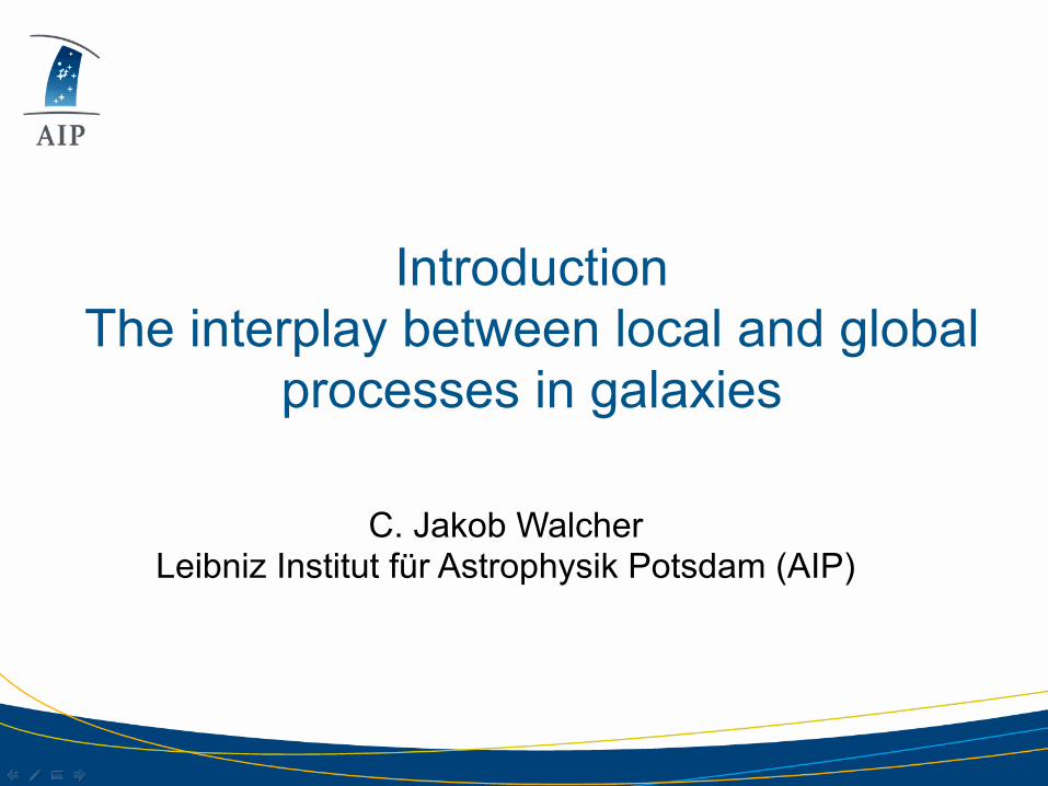
Figure 1 | Disentangling the stellar and dark mass with integral-field stellar kinematics. The top panels show the symmetrized SAURON stellar kinematicsVrms =

√V 2 + σ2 for five galaxies representing a variety of shapes of the kinematics fields, and spanning a range in (M/L)stars values. Here V is the mean

stellar velocity and σ is the stellar velocity dispersion. The middle panel is the best-fitting dynamical model10 with a standard11 dark halo (model b in Table 1). Thebottom panel is a dynamical model where the (M/L)stars was fixed to be 0.65 times the best-fitting one. Where this decrease in (M/L)stars represents the changein mass between a Salpeter and Kroupa IMF. The other three model parameters, the galaxy inclination i, the orbital anisotropy βz and the halo total massM200, wereoptimized to fit the data, but cannot provide an acceptable description of the observations. This plots shows that, for a standard halo profile, the data tightly constrainboth the dark matter fraction and (M/L)stars. The effect would be even more dramatic if we had assumed a more shallow inner halo profile. The contours show theobserved and modelled surface brightness respectively. The values of (M/L)stars and the fraction of dark matter within a sphere with radius equal to the projectedhalf-light radiusRe are printed next to each panel. The galaxy names are given at the top.

0.0

0.5

1.0

1.5

2.0

(M/L

) star

s / (M

/L) S

alp

ChabrierKroupa

x=-2.8 or x=-1.5

no dark-matter halo

Salpeter

a

ChabrierKroupa

x=-2.8 or x=-1.5

best standard halo

Salpeter

b

ChabrierKroupa

x=-2.8 or x=-1.5

best contracted halo

Salpeter

c

1 2 3 4 5 6 8 12(M/L)stars (MO • /LO •)

0.0

0.5

1.0

1.5

2.0

(M/L

) star

s / (M

/L) S

alp

ChabrierKroupa

x=-2.8 or x=-1.5

best general halo

Salpeter

d

1 2 3 4 5 6 8 12(M/L)stars (MO • /LO •)

ChabrierKroupa

x=-2.8 or x=-1.5

fixed standard halo

Salpeter

e

1 2 3 4 5 6 8 12(M/L)stars (MO • /LO •)

ChabrierKroupa

x=-2.8 or x=-1.5

fixed contracted halo

Salpeter (x=-2.3)

f

log σe (km/s)

1.7 1.9 2.1 2.3 2.5

Figure 2 | The systematic variation of the IMF in early-type galaxies. The six panels show the ratio between the (M/L)stars of the stellar component, determinedusing dynamical models, and the (M/L)Salp of the stellar population, measured via stellar population models with a Salpeter IMF, as a function of (M/L)stars.The black solid line is a loess smoothed version of the data. Colours indicate the galaxies’ stellar velocity dispersion σe, which is related to the galaxy mass. Thehorizontal lines indicate the expected values for the ratio if the galaxy had (i) a Chabrier IMF (red dash-dotted line); (ii) a Kroupa IMF (green dashed line); (iii) aSalpeter IMF (x = −2.3, solid magenta line) and two additional power-law IMFs with (iv) x = −2.8 and (v) x = −1.5 respectively (blue dotted line). Differentpanels correspond to different assumptions for the dark matter halos employed in the dynamical models as written in the black titles. Details about the six sets of modelsare given in Table 1. A clear curved relation is visible in all panels. Panels a, b and e look quite similar, as for all of them the dark matter contributes only a smallfraction (zero in a and a median of 12% in b and e) of the total mass inside a sphere with the projected size of the region where we have kinematics (about one projectedhalf-light radiusRe). Panel f with a fixed contracted halo, still shows the same IMF variation, but it is almost systematically lower by 35% in (M/L)stars reflectingthe increase in dark matter fraction. The two black thick ellipses plotted on top of the smooth relation in panel d show the representative 1σ error for one measurementat the given locations. We excluded from the plot the galaxies with very young stellar population (selected as having Hβ > 2.3 A absorption). These galaxies havestrong radial gradients in their population, which break our assumption of spatially constantM/L and makes both (M/L)Salp and (M/L)stars inaccurate.

2

Cappellari et al., 2012


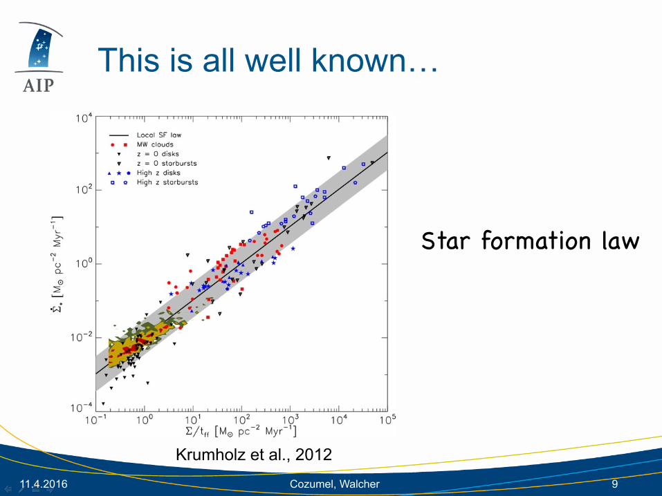
This is all well known…

9

Krumholz et al., 2012

Star formation law


So what do we make of this?

10

A nice conference

Can we do even more?


Can we use this to understand galaxy evolution?

11

There are a few questions that arise:

In order of increasing naivety


What is the right scale?

1) Galaxies are points - they are the entities we study

2) 1 kpc - that is the typical scale we can resolve for large samples (both obs and sim)

3) Probably not one scale to rule them all, but one scale for each process…

12


Is this emergence???

13

The ability to reduce everything to simple fundamental laws does not imply the ability to start from those laws and reconstruct the universe.

Anderson (1972)

Emergence: the arising of novel and coherent structures, patterns and properties during the process of self-organization in complex systems.

Goldstein (1999)Analytical expressions?


What is the right level of complexity???

14

Due to the highly complex and nonlinear physical processes involved in galaxy formation numerical simulations have become the major tool for theoretical progress in this field.

Springel (2016)

But: If you built a computer the size of the universe, with every single atom in it, you could recompute the universe, but you would understand nothing!


On progress in galaxy evolution

• Use simulations to identify analytical laws • Not to reproduce the universe

• Use observations to understand processes • Not to study “pet objects”

• We need a revival of analytic formulations of astrophysical processes

15

11.4.2016 Cozumel, Walcher 16

There is more to discuss.

What does it mean to understand galaxy evolution? -> Debate on Friday

Barbara Catinella, Patricia Sanchez-Blazquez, Klaus Dolag, Vladimir Avila

Documents

Introduction The interplay between local and global ... · Introduction The interplay between local and global ... Our SDSS galaxies have star ... If instead of the considered functional