Introduction of Model Predictive Control COPYRIGHTED MATERIAL

1

Multivariable Predictive Control: Applications in Industry, First Edition. Sandip Kumar Lahiri. © 2017 John Wiley & Sons Ltd. Published 2017 by John Wiley & Sons Ltd.

1

1.1 Purpose of Process Control in Chemical Process Industries (CPI)

Any industrial process, especially oil refineries and chemical plants, must satisfy several requirements imposed by its design and by technical, economic, and social conditions in the presence of ever‐changing external influences (disturbances). Among such require-ments, the most important ones are as follows:

●● Safety: This is the most important requirement for the well‐being of the people in and around the plant and for its continued contribution to economic development. Thus, the operating pressures, temperatures, concentrations of chemicals, and so on should always be within allowable limits.

●● Product quality/quantity: A plant should produce the desired quantity and quality of the final products.

●● Environmental regulations: Various international and state laws may limit the range of specifications of the effluents from a plant (e.g., for ecological reasons).

●● Operational constraints: The various types of equipment used in a chemical plant have constraints (limits) inherent to their operation. Such constraints should be satisfied throughout the operation of the plant (e.g., tanks should not overflow or go dry).

●● Economics: The operation of the plant should be as economical as possible in its utilization of raw materials, energy, and human labor.

●● Reliability: The operation of the plant should be as reliable as possible to ensure that the plant is always available to make products.

These requirements dictate the need for continuous monitoring and control of the operation of a process plant to ensure that operational objectives are met. This is accomplished through an arrangement of instrumentation and control equipment (measuring devices, valves, controllers, computers) and human intervention (plant designers, plant operators), which together constitute the control system.

There are three general classes of requirement that a control system is called on to satisfy:

1) Suppression of disturbances2) Ensuring the stability of the process3) Optimizing the performance of the process

Introduction of Model Predictive Control

0003106549.indd 1 7/12/2017 7:40:48 AM

COPYRIG

HTED M

ATERIAL

1 Introduction of Model Predictive Control2

Traditionally, PID controllers are used in CPI to perform these tasks. PID regulatory controllers efficiently ensure stability of the process and suppression of disturbance. However, due to the multivariable nature of the process and complex interactions between process parameters, PID controllers cannot make a coordinated control move to optimize the process performance. Here lies the need of model predictive control.

1.2 Shortcomings of Simple Regulatory PID Control

PID control forms the backbone of control systems and is found in most CPI. PID control has acted very efficiently as a base‐layer control for many decades. But with increased global competitiveness, process industries have been forced to reduce production costs in order to maximize profit. They must continuously operate in the most efficient and economical matter possible.

Most modern chemical processes are multivariable (i.e., multiple inputs influence same output) and exhibit strong interaction among the variables. Let us consider an operation of a boiler whose main function is to produce and deliver steam to down-stream units or steam header at a specified temperature and pressure. The boiler has a drum with inlet water flow and is heated by fuel gas to produce steam. Now consider a situation where demand of the steam in downstream units increases, and it starts drawing more steam from the header. As a result, water level in the boiler will drop, vapor space above the water will expand, and consequently pressure and temperature will drop. Note that the water level in boilers is not independent and can affect the steam pressure and temperature. As a corrective action, if inlet water flow increases to control level, this will drop the boiler temperature. It will call for more heating and more evaporation, which will again lead to level drop. This demonstrates that there are very strong multivariable interactions among steam pressure, temperature, boiler level, and inlet water flow. Everything affects everything.

Now consider a conventional basic regulatory control scheme in a boiler where multiple single‐input, single‐output PID controllers are used for controlling the plant (multiloop control). Say, boiler level is controlled by inlet water flow, temperature is controlled by fuel gas flow, and boiler pressure is controlled by outlet steam flow. One basic shortcoming of PID loop controls is that they act as a single‐input, single‐output (SISO) controller in an island mode. For example, level controller will see and maintain only level with no idea what is happening with pressure and temperature. The same is true for the temperature controller, which will adjust the fuel gas base on temperature feedback and will not care for level. Now consider the previous situation, where the level starts dropping due to more drawing of steam from header. Level controller will increase inlet water flow, which will reduce the temperature. Temperature controller will increase fuel gas flow, which will again lead to level drop. Again, the level controller allows more inlet water flow to maintain level. There is a lack of coordination among the controllers, and they all act as unconnected islands. Neighboring PID loops can cooperate with each other or end up opposing or disturbing each other. This is due to loop interactions and is a serious limitation of PID regulatory controller. It is very important to understand the multivariable interactions in the chemical process plant and then try to develop model predictive control.

MPC usually stands for model predictive control. Model predictive control is used in multivariable processes where multivariable interactions among the process

0003106549.indd 2 7/12/2017 7:40:48 AM

1.3 What Is Multivariable Model Predictive Control? 3

parameters are significant. However, MPC also stands for multivariable predictive control. MPC is used for both model predictive control and multivariable predictive control throughout this book. In industry, sometimes it is also called advanced process control or APC. Reader should appreciate that MPC stands for all of them in this book and fundamentally they refer to same model predictive control in a multi variable pro-cess environment.

Unlike the PID controller, MPC is a multi‐input, multi‐output (MIMO) controller. MPC receives all the inputs (e.g., temperature, pressure, level, fuel gas flow, inlet eater flow) and uses a predictive model to predict the output. As the name suggests, the heart of MPC is the predictive model. It then calculate the fuel gas flow, inlet water flow and other factors so that the controlled variables (temperature, pressure, level) are main-tained at their set point or within their specified limit. The internal predictive model will account for all the multivariable interactions among the process parameters and adjust the manipulated variable accordingly. This is where MPC is more advantageous than multiloop PID controllers.

Let us consider another example of driving a car on the busy road. The car has two control outputs—namely, speed and direction. The manipulated variables are accel-erator, brake, and steering. Now it must adhere to some safety limits—it cannot leave the road, it has to follow left or right side of the road depending on the country, it must maintain safe distance with other vehicles, and so on. There are some input constraints, also. For example, fuel injection cannot be increased rapidly to very large value.

Now consider two simple regulatory PID‐type controls on the car. Let’s say that direction is controlled by steering and speed is controlled by the accelerator, and these two controllers act independently without knowing each other. As it is well known, while turning on a curved road, speed will decrease—there are interactions between direction and speed. The two independent controllers are just like two drivers running the car, one only looks at direction and other only maintains the speed irrespective of direction, and there is no coordination between them. It would be a disaster, and cars cannot be drive in this manner. Here we need multivariable controller, which will simultaneously measure direction and speed and changes steering, accelerator, and brake simultaneously. This example is given to demonstrate the limitations of PID controllers in multivariable interactive process plant and MPC will be helpful over conventional multiloop PID controller.

1.3 What Is Multivariable Model Predictive Control?

In a process plant, it is only seldom that one encounters a situation where there is a one‐to‐one correspondence among manipulated and controlled variables. Given the relations between various interacting variables, constraints, and economic objectives, a multivariable controller is able to choose from several comfortable combinations of variables to manipulate and drive a process to its optimum limit and at the same time achieve the stated economic objectives. By balancing the actions of several actuators that each affect several process variables, a multivariable controller tries to maximize the performance of the process at the lowest possible cost. In a distillation column, for example, several tightly coupled temperatures, pressures, and flow rates must all be coordinated to maximize the quality of the distilled product.

0003106549.indd 3 7/12/2017 7:40:48 AM


Model predictive control is, as the name implies, a method of predicting the behavior of a process based on its past behavior and on dynamic models of the process. Based on the predicted behavior, an optimal sequence of actions is calculated. The first step in this sequence is applied to the process. For every execution period, a new scenario is predicted and corresponding actions are calculated based on updated information.

The real task of multivariable model predictive control (MPC) is to ensure that the operational and economic objectives of the plant are adhered to at all times. This is possible because the computer is infinitely patient, continuously observing the plant, and prepared to make many, tiny steps to meet the goals.

A definition that seems to provide the best overall description of what is intended is thus:

MPC is the continuous and real‐time implementation of technological and oper-ational know‐how through the use of sufficient computing power in a dynamic plant environment in order to maximize profitability.

1.4 Why Is a Multivariable Model Predictive Optimizing Controller Necessary?

Due to interactive nature of process variables, where change in one affects more than one related variable, it would be ideal to have a controller that is able to combine the operation of a number of single loop controllers. At the same time, this controller should also be able to choose, intelligently, a comfortable selective group of those variables whose manipulation will drive the object variable(s) to its or their optimum targets.

Interaction among process variables is a very common situation encountered in many process plants. Often, the selection of variables to be driven to their limits and extent of their manipulation is left to the subjective judgment, consequent of experi-ence, of operator‐in‐charge. The selection is essentially a trade‐off between variables to be driven to their limits. This is largely because of the complexity of interactions among variables. This judgment, while not wrong from a process or operational viewpoint, may not be in sync with company’s objectives or market demands. Every operator recognizes the interaction among process variables. However, it is the impracticality of negotiating these variables to maintain an optimum condition at all times that forces operators to maintain the variables at a “comfortable” location, away from their constraints. A direct result of this is that the operation is never at its optimum point. This is where a multivariable controller steps in to perform.

Let us understand the concept of process interactions through a distillation column example. Figure 1.1 is a schematic of a distillation column (debutanizer column). In this scheme, there are two primary aims:

1) Reduce butane in column overhead.2) Prevent slip of propane into butane at bottom.

The two concentration levels at top and bottom are themselves interactive. Further, the two are affected by reflux flow, reboiler steam, and variations in feed flow and quality. A variation in feed quality will change bottom composition sooner than it will affect top

0003106549.indd 4 7/12/2017 7:40:48 AM

1.4 Why Is a Multivariable Model Predictive Optimizing Controller Necessary? 5

product. Once the controller senses the change in bottom quality, it will immediately calculate the changes to be made to reflux and reboiler steam flow rates to drive bottom quality to the set target. While arriving at the step values for reflux and steam flow rates that will drive bottom quality, the controller also takes cognizance of the effect of feed disturbance, reflux, and steam flow on top quality. This way, top quality is kept under control.

If the controls were single‐loop controllers, one each for top quality and bottom quality, the column will swing because of interacting effects of change in steam flow and reflux flow on bottom and top qualities. A multivariable control system can also take into account the cost of applying each control effort and the potential cost of not applying the correct control effort. Costs can include not only financial considerations, such as energy spent versus energy saved, but safety and health factors as well.

Once the basic aim of maintaining quality is achieved, the focus can be shifted to achieving economic targets. It is possible to set a constraint (of the more expensive product in cheaper product), thereby minimizing loss of the more expensive product. While forcing the controller toward realizing this goal, it can also be asked to look into the possibility of reducing reflux flow and reboiler duties. All three goals set for the controller are dependent on one another. Yet, because it is a multivariable controller that has already been taught the effect of changing one variable on related variables, it keeps a check of the variables at each move.

FC

FITI

FCLC

LC

QI

QI

MPC withpredictive

model

Figure 1.1 Flow scheme of a simple distillation column using multivariable model predictive controller

0003106549.indd 5 7/12/2017 7:40:48 AM


1.5 Relevance of Multivariable Predictive Control (MPC) in Chemical Process Industry in Today’s Business Environment

Business environment has drastically changed in last 20 years. Globalization, reduced profit margin, and cut‐throat competition among process industries has changed the rule of the game. Making money by safely producing chemicals, petrochemicals, and oil refinery products are not sufficient to survive in today’s business environment. Maximization of profit, continuous improvement of operation, enhanced reliability, and maximization of on‐stream factor are buzzwords in today’s CPI. Industries are shifting focus to energy efficiency, environment friendliness, and sustainability. Capacity maximization by exploiting the margin available in process equipment is no longer a luxury but a necessity. Maximize profit margin by reducing waste product, by increasing mass transfer and energy efficiency of equipment, and by pushing the process at their physical limit are the current trends of CPI. Reduction in oil price, decline in Chinese economy, growing instability in Middle East, and competition from US shale gas, for example, add new dimensions in business environment in recent years. Process industries are experiencing threats to their survival like never before. Stringent pollution control laws, enforcement of energy efficient process, involvement by government agencies, and decline of sales price of end products are some issues that force the process industries to look for new technological innova-tions to do business.

Traditionally, process controls were meant to control the process parameters within their safe boundary limit. This ensures a stable and safe operation. The introduction of sophisticated DCS system in CPI reduces manpower and production costs and increases the ability to monitor and operate the whole process from the control room. Traditional regulatory control (PID control) makes it possible to run the process at its set point given by DCS operator. However, optimization of process parameters to maximize profit depends on the individual operator understanding and efficiency. Online optimi-zation of process, pushing the process at multiple constraints and deriving maximum profit margin, is no longer possible by traditional regulatory control. There is a need for higher‐level control to oversee the scope of optimization. Multivariable process control fits that demand. The real task of MPC is to ensure that the operational and economic objectives of the plant are adhered to at all times.

1.6 Position of MPC in Control Hierarchy

Advance process control nowadays consists of several layers in a hierarchical fashion, as shown in Figure 1.2.

1.6.1 Regulatory PID Control Layer

The bottommost level, which is directly connected with the instruments (transmitters, valves) of the plant, is known as basic regulatory PID control level. PID control has single sensing element and single final control element. That’s why they are called

0003106549.indd 6 7/12/2017 7:40:48 AM

1.6 Position of MPC in Control Hierarchy 7

single‐input, single‐output system (SISO). Simple conventional temperature, pressure, flow control loops along with cascade control, and ratio control are fall under this level. A typical setup consists of a basic instrumentation layer in a DCS system that contains the PID controllers, which send outputs to the control valves in the plant. The primary goals of this base‐level control are fast sensing the disturbance, fast disturbance rejection, and operational stability. Execution time is typically one second or less. PID controllers have been available for decades across chemical process industries and are considered the backbone of the industrial control system.

Long-term scheduling and planning

Plant performance

Average data &constraints of whole plant

Average data & constraints

Measured values

Process

FT

Controller set points

Target

Target

Economics andconstraints

MPC

Real-time optimizer (RTO)

First layer of online optimizer

Basic control loop in DCS

Advance regularatory control layerRegularatory PID loop

Multivariable model predictive control (MPC)

Second layer of online optimizer for multiple MPC

1 – 2 weeks

1 – 2 days

1 – 3 hrs

1 – 3 min

0.3 – 1 sec

Figure 1.2 Hierarchy of plant‐wide control framework

0003106549.indd 7 7/12/2017 7:40:48 AM


1.6.2 Advance Regulatory Control (ARC) Layer

The second layer just above the PID control layer is called the advanced regulatory control. The main feature of this control layer is that most of the time they are multi‐input, single‐output (MISO) systems. A few examples are pressure‐compensated temperature, pressure, temperature, and density‐compensated flow or mass flow, simple feedforward control based on auxiliary measurements, and override or adaptive gain control. Simple inferential process calculation‐based control systems such as heater duty control and distillation tower flooding control also fall under this category. ARCs are typically implemented using function blocks or custom programming capabilities at the DCS level. Execution time is typically one to two seconds. Primary goals are enhanced stability and performance, simple inferential control, and feedforward actions along with feedback control.

1.6.3 Multivariable Model‐Based Control

This type of control is characterized by simultaneous considerations of many controlled variables (CVs) and simultaneously adjusting many manipulated variables (MVs) based on model predictions. That’s why this type of control is called a multi‐input, multi‐output (MIMO) system. The heart of the control is a dynamic model of the process that predicts future paths of control variables. Simultaneous control of more than one CV by coordinated adjustment of more than one MV is a main feature of this control layer.

An MPC is a multivariable model predictive controller that sits above a regulatory control implemented in DCS. In its turn, it receives its set point from a real‐time optimizer. The tree can be extended upward to market forces. In a hierarchical sense, an MPC is a low‐level controller. It takes cognizance of ground‐level realities or constraints and directs basic controllers, already provided, toward an optimum target. The direction or targets can be set by operator or higher‐level optimizers.

The principal aims of an MPC are as follows:

●● Drive variables in a process to their optimum targets keeping in mind the interaction among variables.

●● Effectively deal with constraints.●● Respond quickly to changes in optimum operating conditions.●● Achieve economic objectives.

Typical execution time is one to five minutes. MPC resides in a supervisory computer, which at regular intervals (typically once per minute) scans measured data from the DCS system and then writes set point to the regulatory control loop.

1.6.4 Economic Optimization Layer

Optimization layers sit at the top of multivariable control layer. Optimization again has three layers.

1.6.4.1 First Layer of OptimizationMPC provides first‐level optimization. User normally specifies an economic objective function for the controller and assigns costs or values to its variables. Most of the time, most CVs are not required to control at specific set points; rather, they are required to be maintained between high and low ranges. This gives rise to degrees of freedom,

0003106549.indd 8 7/12/2017 7:40:48 AM

1.6 Position of MPC in Control Hierarchy 9

and the optimizer translates into a direction to move the MVs. Steady‐state optimizer calculates the objective function while obeying the constraints of CV and MV limits. Economic optimizer finds the best position (corner) in the solution space by using the linear program (LP) or quadratic program (QP) method of optimization. These constrained economic optimizers are typically used in conjunction with a multivariable control engine to implement the solution. The multivariable control layer and this first layer of optimizer together are known as model‐based predictive control (MPC). Typical execution time is one to five minutes.

1.6.4.2 Second Layer of OptimizationThis layer sits on the top of first layer of optimization and overlooks any potential opportunity that exists among the different units of a process plant. This optimization algorithm coordinates between different units of the plant, makes use of feedforward or disturbance variables, and tries to optimize the overall plant objective functions instead of individual unit objective functions with an aim to maximize the economic benefit of whole plant.

Each MPC application normally operates independent of the others. In order to optimize the operation of an entire unit, an online optimization system can be installed. MPC can accommodate optimization by slogan on each subplant over which it has control. These systems include calculations to the level of detail of, for example, tray‐to‐tray calculations in distillation columns. In the online optimization system, a profit function taking into account feedstock and energy cost and product prices is maximized for the unit. When calculating the optimum, all product flows from the unit are calcu-lated, taking into account all known unit constraints and the heat integration in the unit.

Based on solutions of overall objective function, it provides set value to the MPC optimizer (first layer), which subsequently implemented it in the plant. Sometimes, running a particular unit suboptimally gives scope to increase profit in other units and this maximizes the overall profit. This particular feature is exploited in the multiunit optimizer. Typical execution frequency is one hour.

1.6.4.3 Third Layer of OptimizationReal‐time optimizer (RTO) is the highest level of optimizer whose job is to optimally shift in operation priorities as per market demand and raw material availability. Just as, for example, fluidized catalytic cracking (FCC) unit of oil refinery is operated to produce different products like gasoline, ATF, and LPG. FCC unit can be operated under many following priorities, as per market demand:

●● Maximization of gasoline or LPG product●● Maximization of ATF●● Maximization of profit●● Minimization of energy consumption

Now these market‐driven operating goals must be achieved while operating condi-tions are also changing. Some examples of operating conditions changes are as follows:

●● Changes in crude oil quality●● Changes in operating conditions due to catalyst performance degradation over time

(low selectivity), heat exchanger fouling, or changes in separation efficiency in distil-lation columns

0003106549.indd 9 7/12/2017 7:40:48 AM


Now in a situation where objective function (operational priorities) and constraints (operating conditions and inputs) are changing dynamically, what is the best way to run the plant (FCC, for example)? Real‐time optimizers (RTOs) address this issue. An RTO has complex algebraic and partial differential equations models of the whole system along with data reconciliation and it solves it dynamically (say, every 16 to 24 hours), while honoring all the operational constraints.

What should be the best operating points amid constraints and as per current market demand? RTO solutions answer this question and implement them in the plant. Solutions of RTO downloaded as external targets in the lower layer and all the lower‐layer optimizers are subsequently implemented in the plant. The optimizer first calculates a base‐case situation that identifies where the plant is currently operating. In a second stage, the optimizer will maximize a profit function, which results in setting the target values for control. The new target set points are downloaded every two to four hours. Via this technique, circumstances of changing economics, varying feed types, and modes can be handled such that a high number of multiple constraints can be met simultane-ously and “hidden” opportunities from distant interactions in the plant can be exploited.

As already seen, advance process control today is a multilevel hierarchical control, solves a variety of problems, and requires large, multilevel technical skills starting with control engineering, planning and scheduling engineers, process engineering, and optimization experts. Today’s process control systems not only keep the process parameters within their desired range but also dynamically move the plant in the most economically optimum zone. They keep recalculating and moving the plant while the economical optimum zone keeps moving from one place to another based on market demand and input constraints.

Figure 1.2 shows the full hierarchy of optimization/process control, as discussed in this section.

1.7 Advantage of Implementing MPC

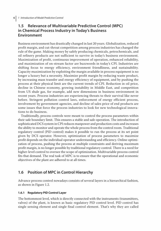
Each type of controller realizes benefits for the user. As we move into realms of greater sophistication, the benefits are more. Figure 1.3 shows some typical benefits associated at each level of control.

Advanced control and optimization benefits are field proven and generate high rates of return on investment. Figure 1.4 shows some typical areas where MPC is used to bring more profit:

●● Increased throughput: A typical 2 to 4 percent throughput increase is very common in industry after MPC implementation. This throughput increase is done while obeying different constraints and limits.

●● Better management of constraints: As MPC has internal dynamic predictive model, it predicts the CVs future value and try to maintain them very near to constraints. In industry, the following constraints are reported to generate high returns:

●● Furnace capacity●● Column flooding and hydraulic limits●● Overhead condenser capacity limitation●● Less flaring

0003106549.indd 10 7/12/2017 7:40:48 AM

1.7 Advantage of Implementing MPC 11

●● Improved yields: MPCs stabilize and optimize the process parameters by their predic-tive capability, which ultimately helps to improve yields, catalyst selectivity, etc.

●● Reduced energy usage: MPCs constantly try to reduce the steam and fuel gas —i.e., energy input to the process by its optimization capability.

●● Decreased operating costs: MPCs always move the process toward its most economic operating zone and hold the process at multiple constraints. It makes it possible to lower pressure operation, adjust fuel gas to oxygen ratio, and make more severe flushing, produce less slops, and so on, and thus continuously decrease operating cost of the unit.

●● Lower pressure operation: Generally, a distillation column operated at lower pressure means better separation and lower energy costs. Column operating pressure is dic-tated by cooling water temperature available to cool light components coming from top. APC can be configured to keep a constant watch on column top pressure or reflux temperature, allowing the column to be operated at minimum possible pressure.

●● Less flue gas oxygen: A typical case of multivariable controller. Target heater outlet temperature is maintained by simultaneously adjusting the fuel rate and airflow rate (or excess oxygen). More oxygen or air implies lower hearth temperatures or higher fuel consumption for the same heater outlet temperatures. Very low excess oxygen implies inefficient combustion or fuel loss.

●● Reduced slop make: APC not only minimizes producing better‐quality product but also avoids making off‐spec product. Hereby, it reduces slop make.

●● Improved quality consistency: MPCs make less quality giveaway against specification. When quality is a critical parameter, it is the general tendency to operate the plant at a condition where the average quality is better than necessary. It is cost to pay for being safe. With APC in place, the swings are reduced. This automatically translates into money due to reduced give away.

●● Increased production of more valuable products: In refineries where high‐value products are occasionally blended with low‐value products, it is imperative that only

00

110

100

100

90

90

80

80

70

70

60

60

50

50

40

40

30

30

Capital investment (%)

Advance regulatory control

Basic control

MPC

Pot

entia

l ben

efit

from

pro

cess

con

trol

(%

)

20

20

10

10

Online optimizer

Figure 1.3 Expected cost vs. benefits for different levels of controls

0003106549.indd 11 7/12/2017 7:40:48 AM

Incr

ease

dth

roug

hput

Bet

ter

cons

trai

nts

man

agem

ent

Impr

oved

yiel

ds

Dec

reas

edop

erat

ing

cost

s

Impr

oved

qual

ityco

nsis

tenc

y

Incr

ease

dop

erat

ing

flexi

bilit

y

Incr

ease

dop

erat

ing

safe

ty

Impr

oved

proc

ess

stab

ility

Red

uced

ener

gy/

utili

ty u

sage

Figu

re 1

.4 T

ypic

al b

enef

it of

MPC

0003106549.indd 12 7/12/2017 7:40:48 AM

1.8 How Does MPC Extract Benefit? 13

the requisite quantity of high‐value product be used. Any excess use is loss. APC, with its smoothening effect, minimizes these losses while maintaining quality target.

●● More stable product quality: MPCs are able to maintain more stable product quality for blending/downstream unit.

●● Increased operating flexibility: MPC uses coordinated movement of multiple MVs to control multiple CVs. It uses the impact of disturbance variables on CVs as a feedfor-ward variable. All these are used to give more flexibility to operate the process plant.

●● Easier and smoother operation with less operator intervention: This will reduce their stress while more rapidly returning the process to normal operations, and it provides a smoother, faster, and better transition between different feed rates.

●● Reduced time off‐spec during grade change of polymer or crude changeover.●● Improved process stability: MPC uses its inherent model to stabilize the process first.

Typically it reduces the standard deviation of key process parameters to 50 percent of pre‐MPC value.

●● Reduced utility consumption (stripping steam, driving steam, air blower, etc.): When a column operates at lower pressures, reboil requirement is reduced.

●● Increased operating safety: This is in direct relation to uptime of MPC. Higher upti-mes signify less operator intervention in process. This reduces chances of error mak-ing process inherently safer.

●● Implementation of APC/MPC: In terms of blend property control and blend ratio control in the blending area, implementation usually results in the following:

●● Reduced quality giveaway●● Optimum use of the more valuable components and additives●● Reduced reblending requirements●● Better usage of the available tankage●● Typical benefits range from US¢ 10–20/bbl. of product●● Reduction of reformer processing severity due to the reduced requirement for

octane achieved by better blend property controls●● Increased blender throughput as the need for reblends is reduced or eliminated●● Potentially huge savings may be realized through reduction in operating incidents

with the use of blending APC solutions

1.8 How Does MPC Extract Benefit?

Process conditions that can be improved dramatically through MPC application are listed in this section.

1.8.1 MPC Inherent Stabilization Effect

MPC first stabilizes the process. If a process is unstable or has poor control on its key parameters, there is always a scope to potentially lose some of the economic benefits that could have been captured if a well‐controlled process were available. MPC uses feedforward information, best use surge volumes available in the plant, and continu-ously taking small incremental steps for preventive and corrective actions to stabilize the process.

0003106549.indd 13 7/12/2017 7:40:48 AM


The immediate effect of making a move while keeping in view the amplitude of move and its consequence is a smoother operation. MPC takes advantage of this. It pushes its controlled variables toward their constraints. This phenomenon is explained in Figure 1.5.

The real benefit from MPC is obtained not just by reducing variations but also by operating closer to constraints, as illustrated in Figure 1.6.

1.8.2 Process Interactions

Modern chemical plants are highly integrated and have large interactions among pro-cess variable. Nowadays, due to intense global competition, plants were designed with large recycle, heat integrated, less design margin, and more. This leads to large interac-tions and makes different process parameters highly dependent on each other. Normal PID regulatory controllers cannot see these interactions and act as independent con-troller in island mode. Due to this highly interactive environment, tighter control is impossible in PID controller level. As MPC knows about the interaction through its MV‐CV‐DV models, it is capable to compensate the interactions with its prediction capability. Thus, MPC allows optimal and tighter control possible.

Profit

Old S.P. New S.P.

CONSTRAINT

Figure 1.6 Reduced variability allows operation closer to constraints by shifting set point

107

105

103

Before MPC Stabilization afterMPC online

Plant capacity limit

Profitincreasedue tohighercapacity

Exploitation, setpointmoved closer to limit

101

99

97

95

93

91

89

Pla

nt c

apac

ity

Figure 1.5 MPC stabilization effect can increase plant capacity closer to its maximum limit

0003106549.indd 14 7/12/2017 7:40:49 AM

1.8 How Does MPC Extract Benefit? 15

1.8.3 Multiple Constraints

Any chemical process has multiple constraints or limits. These limits are posed by equipment hardware limits (like flooding, furnace tube maximum temperature limits, etc.) and process safety limits (like maximum allowable oxygen concentration to avoid flammable region, etc.). This is shown in Figure 1.7. For an efficient operator, it is impossible to run the process at its limit all the time. MPCs predict onset of such constraints and push the process to hit multiple constraints. MPCs maximize profit function reflecting most favorable combination of conflicting constraints. MPC pushes the process out of the comfort zone of individual operator toward the optimum performance while still honoring the plant safety and operating constraints like high and low limits (set points) for CVs, product composition specifications, metallurgical limits, valve output. All constraints are considered and accounted for in the overall control and optimization strategy.

Unmeasurable targets: MPCs can control calculated variables (commonly called soft sensor or quality estimator)—that is, it can control target or constraints that are not directly measured. Examples are distillation tower flooding, tray or down comer loading, compressor efficiency, impurities in product, and so on.

Large delay process: Many commercial chemical processes have large delay in their responses. These delays may be due to large process inventory (like tempera-ture rise after increasing reboiler steam), process itself (e.g., catalyst selectivity change after changing inhibitor or activator feed rate) or may be due to analyzer dead time. As these delays are captured during step test and incorporated inside the MPC model, MPC is better positioned to anticipate the delayed response and control accordingly.

Difference in product value in a multiproduct plant: for a multiproduct plant, product yields can be changed dynamically as per market conditions by utilizing MPC economic

Operating zone

Process safety limit

Quality specification limit

Equipment metalurgical limit

Process parameter limit

Valve output limit

Equipment capacity limit

Figure 1.7 Operating zone limited by multiple constraints

0003106549.indd 15 7/12/2017 7:40:49 AM


objective value maximization. MPCs can exploit its internal optimization capability if such condition exists.

Different mode of operations: MPCs can be modeled to accommodate different regime or mode of operation such as different polymer grade or different quality crude oil processing. MPCs can be used to quickly switch one mode to other online without much disturbance in the process.

Plant load maximization: When all the constraints are within limit, MPC tries to maximize the plant load continuously with small incremental steps. Due to its prediction capability, MPC will do that without violating any major constraints.

Optimization of load distribution between different equipment: As the MPC model has good understanding of constraint limit, it is always possible to allocate feed in such a way in different units so that the most efficient unit utilization can be maximized. It can also be possible to balance column tray load between rectification and stripping section.

Ambient conditions change: Ambient conditions like cooling water temperature and air temperature vary between day–night and summer–winter. For example, low cooling water temperature at winter can increase condensing load in a distillation column condenser, thus providing extra opportunity to increase load in column assuming that condenser heat duty pose a constraint in summer time. MPC is well equipped to exploit any such spare degree of freedom.

Figure 1.8 shows how opportunity is lost in a typical plant by operator actions. MPC can act on this lost opportunity and bring more profit as it is continuously optimizing the plant on a minute‐by‐minute basis.

●● Use of soft sensor: Sometimes reliable analyzers may not exist for quality estimation of a major product. In such situations, soft sensors can be made that will calculate the quality parameters based on other available process parameters. MPC can use these soft sensors readings as a controlled variable and can control the quality based on real time predictions.

Manipulated variablee.g. feed rate

Optimum

Costly operationbeyond constraint

Conservativeoperation

Worst Operator(do nothing)

Time

Best Operator(chase the optimum)

Delay in respondingto extra capacity

Overcompensationfor violation

Advanced control

Winter seasonincreases process

capacity

Summer limits theproduction capacity

$$

$

Figure 1.8 Opportunity loss due to operator action

0003106549.indd 16 7/12/2017 7:40:49 AM

1.9 Application of MPC in Oil Refinery, Petrochemical, Fertilizer, and Chemical Plants, and Related Benefits 17

●● Excessive operator intervention area: During grade change of polymer, excessive operator interventions sometimes needed to carry out sequence of predetermined action. MPC can be utilized in such situations to automate complex series of action consistently without any error.

1.8.4 Intangible Benefits of MPC

One of the major intangible benefits of MPC is to change the mindsets of operators. Before MPC, operators used to monitor process parameters like flow, level, tem-perature, and pressure. After MPC, operator monitor performance parameters like yields, selectivity, specific energy, efficiency, and constraints. Thus, operation staff can better align themselves to company objective such as maximizing profit and pushing the process to its limit. The obvious benefits are that the process becomes more flexible, there is less switchover timing of crude/polymer grade, and there is less off spec production.

Intangible benefits are harder to quantify but can be quite significant, depending on the project under evaluation:

●● Improved process safety: MPC works as a process watchdog and is capable of identifying any problem beforehand, as it has predictive capability.

●● Improved operator effectiveness: After MPC implementations, operators can focus on key operating parameters and plant constraints rather than focusing on every temperature, pressure, and flow value.

●● Reduced downstream unit variability: It has been reported in industry that fewer process upsets are seen in downstream units after MPC implementations.

●● Better process information: As MPC works on plant economics and plant constraints, operators and engineers have better process understanding after MPC implementation. They start to look at the unit as a profit generator rather than as a simple process unit.

All of these benefits cannot be measured by monetary terms, but they have profound long‐term intangible effect on plant economics.

1.9 Application of MPC in Oil Refinery, Petrochemical, Fertilizer, and Chemical Plants, and Related Benefits

MPC has been applied to almost all types of chemical plants since its inception in 1970. MPC application started in chemical plants and oil refineries and then spread to other chemical plants and slowly other branches of engineering. Currently, it is used in robot-ics application, space application, and biochemical plants. Normally, process responses in chemical plants are considered slow; that’s why it started with chemical plants in 1970s, when computers took a long time to calculate online optimization solutions. Over the years, MPC technology passed through many structural modifications, and now it is considered as a mature technology with large applications in chemical, petro-chemical, and refineries across the globe. Bowen (2008) describes an application of advance process control, RMPCT of Honeywell, in crude distillation unit. Similarly, McDonald (1987) gives an application of dynamic matrix control to distillation towers.

0003106549.indd 17 7/12/2017 7:40:49 AM


Wang (2002) describes application of multivariable predictive control technology in atmosphere and vacuum distillation unit. Other good references of various application of MPC in industry are Clarke (1988); Ordys (2001); and Cremaschi (2005).

The typical payback period of an MPC project is six months. Some actual imple-mentation payback periods are given in Table 1.1. Industries across the globe have reported huge profits due to MPC implementations. Table 1.2 and Table 1.3 give some ballpark benefit numbers reported from chemical industry and refinery, respectively (Honeywell Inc. 2008).

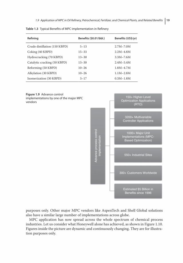
To give the idea of penetration of MPC in the chemical industry, let us consider what one major MPC vendor alone has implemented across globe (refer to Figure 1.9). Figures inside the picture are dynamic and continuously changing. They are for illustration

Table 1.2 Typical Benefits of MPC Implementation in CPI

Petrochemicals Benefits (per year)

Ethylene 2–4% Increase in productionVCM 3–5% Increased capacity/1–4% yield improvementAromatics (50KBPD) 3.4M–5.3M US$

ChemicalsAmmonia 2–4% Increased capacity/2–5% less energy/tonPoly olefins 2–5% Increase in production/Up to 30% faster grade transition

Oil & GasUpstream production 1–5% Increase in productionIndustrial utilitiesCogeneration/Power systems 2–5% Decrease in operating costsPulpingBleaching 10–20% Reduction in chemical usageTMP (Thermos Mechanical Pulping)

$1M–$2M

Table 1.1 Typical Payback Period of MPC

Plants Typical Payback Periods

Oil and gas 1–2 monthsRefining 3–6 monthsChemicals 3–6 monthsPetrochem 4–6 monthsPulping/paper 6–8 monthsIndustrial power 10–12 months

0003106549.indd 18 7/12/2017 7:40:49 AM

1.9 Application of MPC in Oil Refinery, Petrochemical, Fertilizer, and Chemical Plants, and Related Benefits 19

purposes only. Other major MPC vendors like AspenTech and Shell Global solutions also have a similar large number of implementations across globe.

MPC application has now spread across the whole spectrum of chemical process industries. Let us consider what Honeywell alone has achieved, as shown in Figure 1.10. Figures inside the picture are dynamic and continuously changing. They are for illustra-tion purposes only.

Table 1.3 Typical Benefits of MPC implementation in Refinery

Refining Benefits ($0.01/bbl.) Benefits (US$/yr)

Crude distillation (150 KBPD) 5–13 2.7M–7.0MCoking (40 KBPD) 15–33 2.2M–4.8MHydrocracking (70 KBPD) 13–30 3.3M–7.6MCatalytic cracking (50 KBPD) 13–30 2.4M–5.4MReforming (50 KBPD) 10–26 1.8M–4.7MAlkylation (30 KBPD) 10–26 1.1M–2.8MIsomerization (30 KBPD) 3–17 0.3M–1.8M

150+ Higher-LevelOptimization Applications

(RTO)

3200+ MultivariableController Applications

1000+ Major UnitImplementations (MPC-

Based Optimization)

550+ Industrial Sites

300+ Customers Worldwide

Adv

ance

pro

cess

con

trol

impl

emen

tatio

n

Estimated $5 Billion inBenefits since 1996

Figure 1.9 Advance control implementations by one of the major MPC vendors

0003106549.indd 19 7/12/2017 7:40:49 AM

Ref

inin

g p

roce

sses

•Alk

ylat

ion

(40+

)•C

atal

ytic

cra

ckin

g (2

25+

)•C

okin

g (5

0+)

•Cru

de d

istil

latio

n (2

75+

)•H

ydro

crac

king

(60

+)

•Hyd

ro tr

eatin

g (4

5+)

•Iso

mer

izat

ion

(15+

)•L

ubes

(25

+)

•Ref

orm

ing

(100

+)

•MD

con

trol

ble

achi

ng li

me

kiln

•ClO

2 ge

nera

tion

O2

del

igni

ficat

ion

•Dig

este

r (R

&D

) th

erm

o- m

echa

nica

l

•Pul

ping

(T

MP

)

•Aro

mat

ics

•Nyl

on

•Pol

yeth

ylen

e

•Pol

ypro

pyle

ne

•Pol

ysty

rene

•NG

L pl

ants

•Off-

shor

e pr

oduc

tion

•LN

G p

rodu

ctio

n

•But

adie

ne•E

thyl

ene

•VC

M•P

TA

•Eth

ylen

e ox

ide

and

glyc

ol p

lant

•Co-

gene

ratio

n po

wer

/ste

am•A

cetic

anh

ydrid

e

•Met

hano

l

•Am

mon

ia

•Pht

halic

anh

ydrid

e

Pu

lp &

pap

er

Pet

roch

emic

alP

oly

mer

sO

il &

gas

Ind

ust

rial

uti

litie

sC

hem

ical

s

Figu

re 1

.10

Spre

ad o

f MPC

app

licat

ion

acro

ss th

e w

hole

spe

ctru

m o

f che

mic

al p

roce

ss in

dust

ries

0003106549.indd 20 7/12/2017 7:40:49 AM

References 21

References

Bowen, G. X. D. F. X. (2008). Application of Advanced Process Control, RMPCT of Honeywell, in DCU. Process Automation Instrumentation, 4, 013.

Clarke, D. W. (1988). Application of generalized predictive control to industrial processes. IEEE Control Systems magazine, 8(2), 49–55.

Cremaschi, R. A., & Perinetti, J. A. (2005). Implementing multivariable process control. Petroleum Technology Quarterly, 10(1), 115–119.

Honeywell Inc. (2008). Layered Optimization: A low‐risk, scalable approach to driving sustainable plant wide benefits. Optimization Solution White Paper from Honeywell, Inc., USA, April 2008.

McDonald, K. A., & McAvoy, T. J. (1987). Application of dynamic matrix control to moderate‐and high‐purity distillation towers. Industrial & Engineering Chemistry Research, 26(5), 1011–1018.

Ordys, A. W. (2001). Predictive control for industrial applications. Annual Reviews in Control, 25, 13–24.

Wang, C. M., & Lei, R. X. (2002). Application of multivariable predictive control technology in atmosphere and vacuum distillation unit. Petrochemical Technology and Application, 20(5), 321–323.

0003106549.indd 21 7/12/2017 7:40:49 AM

0003106549.indd 22 7/12/2017 7:40:49 AM

Documents

Introduction of Model Predictive Control COPYRIGHTED MATERIAL