1

IATTC-SAMWS

Introduction of a Statistical Age-structured Model Used for Southern Bluefin Tuna in CCSBT

Hiroyuki Kurota and Yukio Takeuchi

National Research Institute of Far Seas Fisheries, Shizuoka, Japan The Commission for the Conservation of Southern Bluefin Tuna (CCSBT) started the development of management procedure (MP) in 2002, which includes a decision rule to determine TAC based on available data such as CPUE series. A MP developed by Butterworth and Mori was selected from several final candidates at the scientific committee in September 2005 and this MP project was almost complete (CCSBT 2005). For evaluating MP performance, an operating model to simulate future population dynamics is necessary. The CCSBT took a long time to develop the operating model besides management procedure itself. Operating models need to reflect actual dynamics of fish population and fisheries with sufficient uncertainty. Thus, development of operating models includes a process of conditioning them on past fisheries data to estimate model parameters, as usually seen in stock assessment models. The operating model used for the SBT MP evaluation originates from a statistical age-structured stock assessment model for the SBT, which incorporates temporal changes in the selectivity (Butterworth et al. 2003). Although it was modified slightly to use as the operating model, the basic concept and the model formulation are not changed substantially. This can be indicated by the fact that the CCSBT continues to use this operating model as one of stock assessment models. Model specification Detailed model specification of conditioning and projection is described in Appendices 1 and 2, which are extracted from documents distributed in the CCSBT. Basic model characteristics are as follows: 1) General target species southern bluefin tuna (SBT) users CCSBT language ADMB Bayesian

grid approach. It assigns weights to results under different assumptions based on prior and/or likelihood. A reference set needs 720 point estimates to be integrated.

MCMC converges used to be “yes” model uncertainty no calculation time over 40 hours (using my laptop PC) No. parameters estimated

571 (for current version. Most of them are selectivity and recruit residuals)

2) Model Structure basic structure age-structured model

2

(convert age into length by a growth curve with variance) spatial pop dynamics no (single stock) sex structured no growth morphs no fishing season events (two seasons per year) fisheries 5 fisheries (longline 1-3, surface, spawning ground) fishing mortality Pope’s approximation natural mortality fixed age specific vectors (grid axis) selectivity smoothness penalties, incorporate temporal variability catchability linear increase (0.5% per year) stock recruitment stochastic Beverton-Holt model

sigmaR (fixed), R0 (estimated), steepness (grid axis) recruit autocorrelation: no (for conditioning), empirical (for projection)

maturity fixed knife edged (age 10) unreported catch allowed for alternative amounts (but without error) 3) Data used catch-effort standardized Japanese longline CPUE (since 1969, five

series, grid) catch at age surface, spawning ground catch at length longlines (Japanese data exists since 1952) tag return yes. Reporting rate is fixed. age-length fixed growth curves depending on cohorts weight-length fixed? discard no environmental data no 4) Likelihood component

Japanese longline CPUE

log-normal likelihood function (The variance is estimated.)

catch at age and length multinominal likelihood function (The sample size is set for each fishery based on sampling intensity.)

tag return data Poisson likelihood function (The variance is fixed.) penalties

recruitment residuals, smoothness of selectivity (random effects are treated as fixed effects)

Eight questions to be discussed Maunder and Hoyle (2005) address eight specific questions that will be discussed during the meeting. The CCSBT has encountered some of these issues in the process of the operating model development. Here we describe current status of the SBT modeling with respect to each question. 1) How to model fishing mortality: Pope’s approximation, effort deviates (MF-CL), solving the catch equation, or virtual population analysis (VPA)-type annual variation in selectivity The SBT model uses Pope’s approximation. It assumes that there are two fishing seasons in a year and each fishery occurs as a pulse annually. This model relies on the

3

separability assumption like other statistical models. The parameterization of selectivity is age-specific and the model structure allows the selectivity ogives to change slowly over time. This assumption of temporal change can give not only flexibility but also instability to the model. Thus, it is a key issue to set amount and frequency of temporal changes. In the SBT model, these parameters are fixed in each fishery considering historical changes of the fishing pattern. 2) How to model selectivity: functional form, smoothness penalties, cubic splines Nonparametric selectivity form is used with constraints by smoothness penalties. The amount of smoothness penalties was fixed by trial and error. The CCSBT tried to use a functional form (double-half-Gaussian function) as a preliminary trial to resolve a convergence problem of MCMC (CCSBT 2004b). However, use of the functional form did not resolve the problem and it was not accepted. 3) Do we need to integrate across random effects (e.g. recruitment deviates) and estimate standard deviations? The SBT model treats random effects regarding recruitment and selectivity as fixed ones, with a penalty added to the objective function based on the distribution assumption. The variance of residuals is fixed. 4) How to estimate uncertainty: Bayesian; profile likelihood; bootstrap; model uncertainty The SBT model adopts Bayesian approach (Punt and Hilborn 1997). At first, the CCSBT estimated parameter uncertainty using MCMC and it worked well. However, when fishery data was updated in 2004, the model had convergence problems. Natural mortality and selectivity estimates showed undesirable results. Although this is probably due to model instability rather than an issue with the ADMB, there was not sufficient time to identify exact causes. Instead, a new simpler approach called the grid approach was used to integrate uncertainties of critical factors into a reference set including 2000 replicates for projection (also see Appendix 2, CCSBT 2004). Since this approach considers only a limited number of uncertainty factors, uncertainties may be underestimated. However, we adopted it as the second best. To estimate uncertainty with this approach, first we selected seven grid axes of uncertainty such as fundamental parameters (e.g. steepness, natural mortality, CPUE-abundance relationship), structural assumptions (e.g. age-specific catchability, sample size) and input data (e.g. different CPUE series). Then we set two or three different fixed values or assumptions in each axis and obtained a point estimate (MPD) for each combination (cell) of those. Finally, each estimation result was assigned a weight depending on prior (steepness, catchability, CPUE, sample size), likelihood (natural mortality) or combination of the two, posterior (CPUE-abundance relationship). The weight determined the number of replicates to be simulated from each estimation result to produce a total of 2000 replicates, a reference set.

4

By using the grid approach, the CCSBT was released from the convergence problem. However, this approach is as computationally intensive as MCMC. This grid approach takes over 40 hours to calculate all 720 cells. 5) How to include environmental data The SBT model does not use environmental data directly as input data. However, in order to take the regime shift of the Aleutian low in 1977 into consideration (but the mechanism is not obvious), different values for R0 (stock-recruitment scale parameter) before and after the year were applied as one of sensitivity tests. The value of estimated R0 for the later years was about half the value for the earlier years. 6) How to perform forward projections The SBT model was developed as an operating model for management procedure evaluation. Therefore, projection specification was determined carefully to test management procedures under more realistic conditions (Appendix 2). Following the classification of uncertainty in projections by Maunder and Hoyle (2005), the reference set integrated by the grid approach covers the uncertainty in estimating the current status and population dynamics. As for the stochastic uncertainty about future conditions, process error in stock-recruitment ( Rσ ) is considered. In particular, because a sudden drop of recruitments after 2000 is a matter of serious concern for the SBT management, recent recruitments are modeled in detail to cover enough uncertainties. This is the reason the projection model assumes autocorrelation in the recruit residuals and stochasticity for the initial number of young fish under age 4 at the beginning of the projection. 7) What likelihood functions to use for different data sets and how to weight data sets in the assessment Objective function consists of three likelihood components for data fits and penalties for recruit residuals and selectivity changes. Total catch estimates for each fishery are assumed to be without error. The log-normal likelihood function is used for Japanese longline CPUE index and the variance parameter is estimated though the fitting procedure. The fit to tag return data is based on an approximation to the Poisson distribution. The variance is fixed in advance. For fitting to age- or length-frequency data, the multinominal likelihood is assumed. The sample size is basically determined based on historical sampling intensity, which is different among years and fisheries. However, there was considerable discussion on how to determine reasonable values of the sample size, and a certain amount of trial and error were required. Alternative error structures such as robust normal likelihood (Fournier et al. 1998) and the log-normal distribution with additional process error were explored in the final phase of the model development. However, due to time constraints, they were not examined adequately. It should be further explored in the future.

5

8) Should we use spatial structure in the population dynamics or are spatially-defined fisheries adequate? The SBT model does not have spatial structure in the dynamics, although fisheries are grouped based on selectivity, which has some connection to fishing ground. This is partly because the SBT has the only spawning ground and it is regarded as a single stock. However, some fishery data and archival tagging data indicate that the SBT has some site fidelity. It may be necessary to include spatial structure explicitly in some way in the future. What we learned from the SBT modeling The stock assessment group (SAG) conducted stock assessment through this age-structured model in September 2005 to finalize the operating model for MP evaluation (Figure 1). Future projection results under current levels of catch indicated that the SBT stock biomass would further decline if nothing was done. Therefore, the Scientific Committee recommended significant quota reduction to the Commission before implementation of MP in 2008 or 2009. Complex statistical stock assessment models are highly valuable to integrate many kinds of information and estimate uncertainties. However, at the same time, model structures and assumptions tend to be too complicated to examine model validity appropriately within limited time. Also there is a possibility that over-parameterization may result in instability of model behaviours. The CCSBT often encountered difficulties that assessment and projection results were sensitive to minor changes of arbitrary assumptions and data. For example, results varied greatly depending on which longline CPUE series was used among five series, which looked quite similar. Also the shape of selectivity curve for Indonesian fishery was one of key issues that influenced results significantly, but there was little information and knowledge on it. Although such difficulties may reflect shortage of data and knowledge on population dynamics, it will be risky to conduct stock assessment within limited time using such models. Therefore, we consider it important to examine model behaviours in advance and eliminate redundant parts to make models slim and reduce calculation time. References Butterworth, D.S., Ianelli, J.N., and Hilborn R. (2003) A statistical model for stock

assessment of southern bluefin tuna with temporal changes in selectivity. African Journal of Marine Science 25, 331-361.

CCSBT (2004a) Report of the Special Management Procedure Technical Meeting. 15-18 February 2004, Seattle, USA.

CCSBT (2004b) Report of the Fifth Meeting of the Stock Assessment Group. 6-11 September 2004, Seogwipo City, Jeju, Republic of Korea.

CCSBT (2005) Report of the Sixth Meeting of the Stock Assessment Group. 29 August – 3 September 2005, Taipei, Taiwan.

Fournier, D.A., Hampton, J., and Sibert, J.R. (1998) MULTIFAN-CL: a length-based, age-structured model for fisheries stock assessment, with application to South Pacific albacore, Thunnus alalunga. Can. J. Fish. Aquat. Sci. 55, 2105-2116.

6

Maunder, M. and Hoyle, S. (2005) Stock assessment methods background. IATTC stock assessment methods workshop. 7-11 November 2005, La Jolla, USA.

Punt, A.E. and Hilborn. R. (1997) Fisheries stock assessment and decision analysis: the Bayesian approach. Reviews in Fish Biology and Fisheries 7, 35-63.

7

1940 1960 1980 2000 2020

05

1015

2025

Rec

ruits

(mill

ions

)

1940 1960 1980 2000 2020

020

040

060

080

010

00

Spa

wni

ng s

tock

bio

mas

s (t

hous

and

tonn

es)

Figure 1. Stock assessment and projection results of the southern bluefin tuna. The projection was conducted under current levels of catch.

8

Appendix 1: A model specification distributed to CCSBT in June 2004 (by courtesy of Vivian Haist)

CONDITIONING MODEL FOR SBT MP TESTING (sbtmod7.tpl, June/04)

THE AGE-STRUCTURED POPULATION MODEL

Population Model

The SBT are modeled with age-specific dynamics. Fishing and natural mortality are treated as discrete events and two seasons are modeled for each year. The population dynamics are:

1 2

1

1 2

1 2

1, 1 1 2

1, , 1 , , 1 , , 1

1 1 for 0 -2,

1 1

1 1

a

m

My a ya fya fya n n

f f f f

My m y m f y m f y m

f f f f

ym fym fymf f f f

N N H H e a m y y y

N N H H e

N H H

−

−+ +

∈ ∈

−+ − − −

∈ ∈

∈ ∈

= − − ≤ ≤ ≤ ≤

= − − +

− −

∑ ∑

∑ ∑

∑ ∑ 1 2 for mMn ne y y y−

≤ ≤

1,0 1y yN R+ +=

1

* 21aM

ya ya fyaf f

N N H e−

∈

= −

∑

fya fya fyH s F=

1

2

*

for

for

1 if in numbers

if in biomass

fyfy

fya fya yaa

fyfy

fya fya yaa

fy

fya

fya fy

CF f f

v s N

CF f f

v s N

Cv

w C

= ∈

= ∈

=

∑

∑

where: yaN is the number of fish of age a at the start of year y,

*yaN is the number of fish of age a at mid-year y,

aM denotes the natural mortality rate on fish of age a, fyC is the catch of fish (numbers or biomass) in fishery f in year y,

fyF is the age-averaged fishing proportion of fishery f in year y,

9

fyaH is the fishing proportion of fishery f in year y for fish of age a,

fyas is the standardized selectivity of fish of age a in fishery f in year y,

fyaw is the average weight of fish of age a in year y in fishery f ,

yR is the age-0 recruitment in year y,

1f is the set of fisheries that occur in the first season (I33),

2f is the set of fisheries that occur in the second season (I33), and m is the maximum age considered (I6, taken to be a plus-group). 1 2,n ny y are the first (I1) and the last (I2) years for the stock reconstruction. Note that solutions are constrained so that the maximum harvest rate on an age-class during a fishing season is 0.9. For the MP reference case the maximum age considered, m, is 30.

Stock-Recruitment

The number of recruits at the start of year y ( )yR is related to the spawning stock size by a

stochastic Beverton-Holt stock-recruitment relationship. The relationship includes a parameter that allows for depensatory effects and has the option for serial correlation (AC) in a terminal sub-set of the residuals:

( ) ( )2

0

1

ln 0.5exp /2 1 exp

if no AC

if AC and

if AC and

ry y

y y Rr ry

y

y y AC

y y AC

S SR

S B

y y

y y

ατ σ

β ν

δ

τ δ

ϖτ δ−

= − − +

= ≤ + >

where yS is the spawning stock biomass in year y,

,r rα β are Beverton-Holt stock-recruitment parameters for regime r,

yτ is the stock-recruitment residual for year y, 2~ 0,y RNτ σ ,

ν is a depensation parameter (I23), ( Note that setting ν at a very small number corresponds in the limit to no depensation),

roB is the equilibrium spawning stock biomass expected during regime r in the

absence of fishing, yδ are stock-recruitment residual parameters estimated in the fitting procedure for

years 1 2 1n ny y y> ≤ + ϖ is the empirical serial correlation in the recruitment residuals,

( )( )1Cor( , ) 1966 3y y ACy yϖ τ τ −= ≤ ≤ − ,

ACy is the year initiating the serial correlation in the stock-recruitment residuals (must be 1996 or later to activate this option, I13).

Spawning stock biomass is estimated as:

10

( )1

ms

y a ya yaa

S b w Nκ

=

= ∑

where ab is the proportion of fish of age a that are mature, s

yaw , the spawning weight at age a

in year y is assumed to be the same as the mean weight-at-age for the Indonesian spawning fishery, and κ is the exponent for a non-linear relationship between body size and reproductive potential (I24). Note that all these parameters, ab , s

yaw , and κ are specified as

model inputs. In order to work with parameters that are more meaningful biologically, the stock-recruitment relationship is reparameterized in terms of the equilibrium spawning biomass expected in the absence of fishing, 0

rB , and the “steepness”, h, of the stock-recruitment relationship (steepness is defined as the fraction of the average spawning biomass expected in the unfished stock, which is obtained when recruitment is 20% of the recruitment expected in the unfished stock):

( )00 14 and

5 1 5 1

rrr r B hhR

h hα β

−= =

− −

where

( ) ( )( ) ( )( )( )

( )1 1

11 '1 ' 0

0 0 , ' ,' 01

exp/ exp

1 expn n

mm aa ar r s s

a y a a m y mama

MR B b w M b w

M

κ κ

−−

− =

==

− = − + − −

∑∑ ∑ .

Only a very limited regime shift option is currently coded in the SBT conditioning model. When the regime shift option (called carrying capacity) is invoked (I8b), an alternate stock-recruitment relationship, based on a different 0

rB , is used from 1978 onward. The two regimes share a common steepness parameter.

Selectivity Ogives

The parameterization of selectivity is age-specific and the model structure allows the selectivity ogives to change slowly over time. Fishing selectivity is parameterized as:

1, ,,

0 for

for

for and

0 for and

cmaxsf

minsf

mins maxsfa f f

maxs ff y aff a

maxs ff

a a

a a as

a a f z

a a f z

λ

λ

< ≤ ≤′ = > ∈ > ∉

( )1

1

1

, ,, ,

, ,

1c

maxsc f

cminsf

maxs minsf f f y a

f y a a a

f y aa a

a a ss

s=

=

′− +=

′∑

11

( ) ( )2

, 1,

exp for , ~ 0,

for

fy

ffya fya fya S

f y af

fya

s y c Ns

s y c

γ γ σ+

∈′ = ∉

( )1maxsf

minsf

maxs minsf f fya

fya a a

fyaa a

a a ss

s=

=

′− +=

′∑

where and maxs mins

f fa a are the minimum (I34) and maximum (I35) age-classes for which

selectivity parameters are estimated for fishery f, fz is the set of fisheries for which age-classes greater than maxs

fa have the same selectivity as age-class maxsfa (I36), fc is the set of

years in which the fishing selectivity ogive can change for fishery f (non-zero I40), and fyaγ

reflects the amount of change in the age effect of fishery f for age a, and 1cy is the first year in which there is catch data (I3).

The stochastic error terms, ftaγ are treated as free parameters subject to the constraints of

their input variances, 2fyS

σ (I40). If the age effects of fishing ( fyas ) are constant over time,

this results in a decomposition of the fleet-specific fishing mortality rate into an age component and a year component. This assumption creates what is known as a separable model. If the age effect of fishing in fact changes over time, then the separable model can mask important changes in fish abundance. The constraints imposed through the variance terms can restrict the selectivity to change only slowly over time, thus improving the ability to estimate the fyaγ ’s. Also, to provide smoothness in the age component there is a curvature

penalty on the age-specific coefficients. This can be based on either the logarithm of the selectivity parameters (I38=0), or a non-negative power of the selectivity parameters (I38>0):

( )( )I38

I38 = ln for

for

0

I38 > 0

fya

fya

fya

sx

s

=

Then a penalty term, based on either squared second-differences or squared third-differences, is added to the negative log-likelihood function for each fishery:

( )

( )( )

( )( )

1

1

22, , 2 , , 1

2,

2

23, , 3 , , 2 , , 1

2,

I39 2

for 2

;

3 3

= 2

I for 39 2

= 3

maxsf

f mins fc f

f

maxsf

f mins fc f

a af y a f y a fya

y y c a a bf

fya ba a

f y a f y a f y a fya

y y c a a b

x x x

g x

x x x x

σ

σ

σ

= −+ +

∈ =

= −+ + +

∈ =

− +

=

− + −

∑ ∑

∑ ∑

This prevents irregular shifts between adjacent age classes. A selection of the third differences penalty function encourages selectivity to be dome-shaped with age while the second difference penalty function favours linear behaviour with age.

12

Growth

Growth is not estimated in the model, but is fixed with assumed known length-age relationships. The mean length-at-age is input for each year, so growth can change over time. Also, fixed length-weight relationships are assumed for each fishery. The length frequency distributions for each age are calculated assuming normal distributions. The standard deviation ( aσ ) of length-at-age is linearly related to the mean length-at-age ( aµ ) based on the

relationship of Kolody and Polacheck (2001): ( )12. 30a aσ µ= + .

Natural Mortality

Age-specific natural mortality can either be specified through input vectors or estimated through the minimization process (I8a). When estimated, the SBT MP model parameterization is used. In that case, two parameters, representing the instantaneous natural mortality at ages 0 and 10 are estimated. A fixed curvilinear function interpolates between those age-specific estimates:

( )0.7

0 10 00.7

10

for 0 1010

for 10a

am m m aM

M a

+ − ≤ ≤=

>

where 0m is the natural mortality rate for age 0 fish and 10m is the natural mortality rate for age 10 fish.

Tagging Model

The dynamics for fish that are tagged and released are assumed to be the same as those for the general population. The tag releases have generally occurred near the beginning of the calendar year (January) so they are treated as discrete events occurring between the two fishing seasons. Because the tagged fish will not be completely mixed during the season following their release it is not assumed that they have the same vulnerability to the immediate fisheries as the general population. Rather, the number of tags released are adjusted for recoveries that occur during the season immediately following their release. The dynamics for the tagged fish are described by:

1 2

0

1, 1

0 for 8 and 1992 1997

1 1 +

yaa a

ya

M My a ya fya fya ya

yaf f f f

T a y

rT T H H e G eυ

− −+ +

∈ ∈

= ≤ > >

= − − −

∑ ∑

for 0 a 7 and 1992 1997y≤ ≤ ≤ ≤

1

* 21aM

ya ya fyaf f

T T H e−

∈

= −

∑

where: yaT is the number of tagged fish of age a at large in the population at the

start of year y, *

yaT is the number of tagged fish of age a at large in the population at mid-

year y, yaG is the number of fish of age a tagged and released at the start of year y,

13

0yar is the number of fish of age a tagged and released at the start of year y

and recovered in year y, yaυ is the reporting rate for fish of age a in year y (I15).

Catch Underreporting

The SBT conditioning model contains a single option for underreporting of historic catches. When this option is selected (I42) the values input for the catches in each fishery and year are increased. For years up to and including 1990 the catches are increased by 5%. For 1991 and onward the input catches are increased by 15%.

PREDICTED QUANTITIES

Catch-at-age and Catch-at-length

Observations of either catch-at-age or catch-at-length are available for each of the fisheries, and are fitted in the model. The predicted catch-at-age a in fishery f and year y is:

1

* 2

ˆ for

ˆ for

fya fya fy ya

fya fya fy ya

C s F N f f

C s F N f f

= ∈

= ∈

For fisheries with length-based data, the predicted catch-at-length l in fishery f and year y is given by:

1 2ˆˆ for , 1 ; for , 2tfyl yal fya

aL p C f f t f f t= ∈ = ∈ =∑

where t

yalp is the proportion of fish of age a that are length l in season t. The tyalp are

calculated assuming normal distributions for length-at-age with known means and variances.

CPUE

Catch per unit effort (CPUE) is fitted as an aggregate index (i.e. not age based) for the LL1 fishery only. The relationships between CPUE and abundance and between CPUE and effort allow for a number of non-linear effects. These effects are not estimated in the model fitting procedure, but rather are determined by control parameters input by the user. The predicted

CPUE in year y ( )ˆyI is given by:

( ) 2 2

2 2

2

ˆ 1 I I

I I

y y y yy y y

y y

E E E EI q q N

E E

ωζ φ

− − = + +

%

14

2

1

*

4

2 1

where for LL11

( 1)

and for LL1

a mfya

y yaj aa

fyjj a

fyy

y

sN N f

sa a

CE f

I

ψ

=

==

=

= = − +

= =

∑∑

%

Input parameters specified by the user are: ζ (I17), φ (I18), ω (I19), ψ (I20), yq (I16),

1a (I21), 2a (I22). The only parameter in the above equations that is estimated through the minimization is q , the catchability when yq =1.

Tag Returns

The predicted number of tag recoveries for each fishery is a function of the number of tagged fish in the population and fishing mortality:

1

* 2

for

for

fya fya fy ya

fya fya fy ya

r s F T f f

r s F T f f

′ = ∈

′ = ∈

where fyar′ is the predicted number of recoveries of fish of age a in fishery f in year y. The

expected number of tag returns in year y is dependent on the tag reporting rate ( )I15, yaυ :

ya ya fyaf

r rυ ′= ∑ .

OBJECTIVE FUNCTION

Likelihood Components for Data Fits

The model is fitted to a CPUE index series, fishery catch-at-age and catch-at-length data, and tag return data. The estimates of total catch for each fishery are assumed to be without error. The negative of the log-likelihood (-lnL) for each of the data components are described below. Note that constant terms of the negative log-likelihood are ignored. CPUE data The likelihood is calculated assuming that the observed abundance index (I14) is log-normally distributed about its expected value with variance 2

Iσ :

( )( ) ( )( )

2

1

2

2

ˆln lnln ln

2

I

I

y y

y yy y

I II

I IL n σ

σ

=

=

−− = +

∑

15

where 1 2 and I Iy y are the first (I4) and the last (I5) years with CPUE data and In

( )2 1 1I I In y y= − + is the number of CPUE observations. The variance parameter, 2Iσ , is

estimated through the fitting procedure, assuming a normal distribution with a minimum

value of ( )20.1 . Catch-at-age and catch-at-length For fitting to catch-at-age and catch-at-length data a multinomial sampling distribution is assumed. Under this assumption, the log-likelihood function for the catch-at-age or catch-at-length data (in numbers) from each fishery can be written:

( )ˆln ln fy fyk fyk

y kL n p p− = ∑∑

where k = a for catch-at-age data, k = l for catch-at-length data, fyn is the effective sample

size for fishery f in year y, and

ˆˆ, for age-based dataˆ

ˆˆ, for length-based dataˆ

fya fyafya fya

fya fyaa a

fyl fylfyl fyl

fyl fyll l

O Cp p

O C

O Lp p

O L

= =

= =

∑ ∑

∑ ∑

.

The ˆ ˆ, , ,fya fyl fya fylO O C L are the observed and predicted catch-at-age or catch-at-length for

fishery f. The effective sample sizes, fyn , are quantities input for each fishery and year (I41).

Different methods are used for inputting age-frequency and length-frequency data in the SBT conditioning model code. Input of length-frequency data is hard-wired such that the code expects input of data for 110 length-frequency bins each of 2cm width and beginning at 32cm. The user controls the fitting of these data by specifying the minimum length category fitted in the model (I25, fish in bins of smaller length than the minimum are aggregated in the first bin), the width of the length bins used in the fitting procedure (I26, best to specify this in 2 cm increments, consistent with how the data is input), and the number of bins used in the fitting (I27, note that any fish of length greater than the length of the terminal bin are aggregated in the terminal bin). The specified binning values apply to the length-frequency data from all fisheries. An additional option allows for fishery-specific aggregation of a specified number of the smallest length bins seen by the model (I28). For age-frequency data, the data input controls the age range in the model fit. For each fishery with age-frequency data (I29 and I30) the user specifies the minimum (I31) and the maximum (I32) ages in the data set. The only aggregation of age-classes that is allowed is when the maximum age specified for fitting the age-frequency is the same as the maximum age in the model, which is a plus group. Tag Returns The fits to the tag return data is based on an approximation to the Poisson distribution. If the tag recapture process is governed by a Poisson distribution, a square root transformation will

16

produce variables that are approximately normally distributed with a standard deviation of 0.5. The negative log-likelihood used in the SBT model is:

( )2

2

ˆln

2ya ya

Ty a

r rL

σ

−− = ∑∑

where yar is the number of tag returns of age a in year y which have been at liberty for more

than one year. In practice the distribution of tag recoveries is likely over-dispersed relative to the Poisson assumption, so the user can specify the variance, 2

Tσ , used in the model fit (I24b).

Likelihood Components for Priors

Stock-recruitment relationship The stock-recruitment relationship used in the SBT model requires prior assumptions about the stock-recruitment steepness parameter, the magnitude of the change in carrying capacity, and the magnitude of the recruitment residuals. The steepness parameter can either be fixed (I9<1) or estimated in the analysis (I9 ≥ 1). When estimated, the steepness is assumed to be normally distributed 2~ ,0.1h N h

% , but the user can specify a tighter area of support (i.e

bounds, I10 and I 11) than would be expected for a normal distribution. The negative log-likelihood for the steepness prior is:

( )( )

2

2 2 0.1

h h− %where h% = 0.5*(I10+I11)

A normal distribution (in log space) is also assumed for the stock-recruitment residuals,

2~ 0,y RNτ σ . The variance of the residuals can either be fixed (I12 <1, Rσ =I12) or

estimated (I12 ≥ 1). In either event, the negative log-likelihood for the normal distribution prior is:

( ) ( ) 1

12

12 1 21 ln

2

ny y

yy y

n n RR

y yτ

σσ

= +

= +− + +∑

.

Note that when estimated there is a lower bound of 0.4 on the Rσ parameter. An uninformative prior is assumed for the change in the carrying capacity (ie. uniform), so the contribution to the objective function is a constant. Selectivity The age-specific selectivity parameterization incorporates two type of assumption that reflect prior belief about the form of the selectivity function. For all fisheries either a dome-shaped or linear relationship between selectivity and age can be specified. The negative log-likelihood for the prior is: ( )2; f

ffya b

fg x σ∑

17

where the variance term, 2

fbσ (I37), reflects belief about the degree to which the selectivities

for fishery f follow the expected shape (domed or linear). For some or all fisheries, the age-specific selectivity functions can change over time. The amount of change is controlled by input parameters (fishery and year specific, I40) related to

the variance of the changes ( )2f

ySσ .

( )2

22f fy

fya

f y c S

γ

σ∈∑ ∑

where fc is the set of years in which selectivity changes for fishery f. Note that for fisheries with time-invariant selectivity this set will be empty. Natural Mortality Additional components of the likelihood function occur when the option to estimate natural mortality is selected (I8a=0). In that case normal prior distributions are assumed for both the

0 10 and M M parameters ( )0 2 10 2~ N 0.4,0.04 ; ~ N 0.1,0.06M M . The negative log-

likelihoods for these priors are:

( )( )

( )( )

2 20 10

2 2

0.4 0.1 and .

2 0.04 2 0.06

M M− −

18

Table 1. Fixed quantities determined through model inputs. Quantity Description Control file code

1 2,n ny y first and last years for reconstruction I1, I2

1cy first year for catch data I3

1 2,I Iy y first and last years for CPUE index data

I4, I5

ACy the year that initiates serial correlation in the stock-recruitment residuals

I13

m last age class in model I6 number of fisheries I7

,mins maxsf fa a minimum and maximum age-class for which selectivity

parameters are estimated for fishery f I34, I35

1 2,f f the set of fisheries in season 1 and in season 2 I33

fc the set of years in which selectivity changes for fishery f I40 fz the set of fisheries where selectivity for fish older than

maxsfa is equal to that of maxs

fa I36

1 2

, , , ,, ,yq a a

ζ φ ω ψ

parameters determining the relationship between CPUE and stock abundance

I16, I17, 118, I19, I20, I21, I22

ν stock-recruitment depensation parameter I23 κ parameter for non-linear body weight-reproductive potential

relationship I24a

h stock-recruitment steepness parameter (Note: also can be estimated)

I9 ≥ 1, then ( )0.5 I10+I11h =

aM natural mortality (Note: also can be estimated) I8a 2Tσ variance of the tag recovery residuals I24b 2Rσ variance of stock-recruitment residuals (Note: can be

estimated) I12<1

2fbσ variance for the shape of the selectivity function for fishery f I37

2f

ySσ variance of the selectivity change in year y for fishery f I40

fyn multinomial sample size for length or age sample from

fishery f in year y I41

Table 2. Quantities “hardwired” in code (i.e. you will need to change the code if you want to change these) Quantity Description

ab proportion of fish mature at age a

fyaw mean weight at age a in fishery f in year y – dependent on input mean lengths-at-age, but weight-length relationship for each fishery is hardwired

syaw mean weight of spawning fish at age a in year y is set equal to mean weight-at-age

for fishery 1 (LL1 fishery) ϖ empirical S-R residuals correlation used in “hard-wired” AC is based on residuals

from 1966 to ( )3ACy − I13.

19

Table 3. Quantities estimated through the function minimization. Note that with the exception of the stock-recruitment steepness parameter and the variances of the stock-recruitment residuals and the selectivity changes, the prior distributions are “hardwired” in the code. (ie. you will need to change the code if you wish to change the prior). Quantity Description Prior

0rB Equilibrium spawning stock biomass in the absence of

fishing for regime r [ ]0 ~ 0,rB U ∞

h stock-recruitment steepness (Note: can also be a fixed quantitiy)

( )

2~ , 0.1

0.5* I10+I11

h N h

h

=

%

%

q catchability [ ]~ ,q U −∞ ∞ 0m natural mortality at age 0 0 2~ 0.4, 0.04m N

10m natural mortality at age 10 10 2~ 0.1, 0.06m N

yδ parameters related to the stock-recruitment residuals – note that the prior distribution is for the s-r residuals, yτ , not the

estimated parameters

2~ 0,y RNτ σ

faλ selectivity parameter for age a in fishery f [ ]~ 0,fa Uλ ∞

fyaγ logarithm of the parameter governing the change in selectivity at age a in year y and fishery f

2~ 0, fy

fya SNγ σ

2Iσ variance of the CPUE index data [ ]2 ~ 0.1,I Uσ ∞ 2Rσ variance of stock-recruitment residuals (Note: also can be

fixed) [ ]2 ~ 0.4,R Uσ ∞

20

Appendix 2: Configuration of the SBT model for the reference set (excerpt of attachment 5 in CCSBT (2004b)).

Specification of grid axes:

Axis Levels Values Prior Simulation

Weights Steepness 3 0.385 0.55 0.73 0.2, 0.6, 0.2 Prior

M0 3 0.3 0.4 0.5 Uniform Posterior M10 2 0.1 0.14 Uniform Posterior

Omega 2 0.75 1 0.4, 0.6 Posterior CPUE 5 Uniform Prior

q Age-range 2 4-18 8-12 0.67, 0.33 Prior Sample Size 2 Panel Original/2 Uniform Prior

Note: when different series are used in conditioning, the MPs tested in projections will still use the median CPUE for the historical period.

Process for assigning weights and integrating over grid cells

The approach used to assign weights to the different cells differs depending on the grid axis, as detailed in the Table above. For some axes (M0, M10 and omega) the weights are based on Likelihood × prior. In other axes, the prior weights override the likelihood. The latter is the case of all factors related to changes in data input (CPUE series and sample sizes), and also the case of the steepness parameter. Given problems in model structure, the likelihood was not considered an adequate basis to assign weights to steepness. In particular, the lack of account for autocorrelation in recruitment in the likelihood and the use of a Beverton-Holt curve were discussed in connection to steepness. Once weights are assigned, the code samples cells with probabilities based on these weights. In order to assure adequate coverage on the steepness, CPUE and sampling size axes, the number of realizations for each h ×CPUE×SS stratum is fixed and values for other axes are sampled within each stratum. Sample sizes are computed as separate grids and outputs are combined in the *.grid file but they are not randomized. In case users want to use only a subset of the 2000 realizations (e.g. 500 to start tuning procedures), they will need to randomize the records to avoid biases due to the change in sample size assumptions.

Basic model assumptions

Projection period: 2004-2031 (last biomass computed for beginning of 2032) Catch split: based on average of 2001-2003

21

Selectivities

Conditioning - LL1 selectivity changes (CV=0.5) every 4 years, with change in 1997 and 2001 (last

block is only three years). - LL2, LL3 and LL4 are constant. - Indonesian selectivity is constant up to 1996 when it starts changing every two years

with CV=0.5. - Australian selectivity changes (CV=2) by blocks of 4 years up to 1997 when it starts

changing every year.

Projections Randomness in future selectivities were added so that the age-composition data were not unrealistically informative. Random-walk processes as assumed in conditioning are not appropriate because they may result in the selectivities wandering off into implausible regions. The following lognormal formulation is used for LL1 fishery (note that first subscript corresponds to fishery f=1): ,

1, , 1, ,2003ea y

a y as s ε= for ss aaa max1

min1 ≥≥ where 17,2 max

1min1 == ss aa

yy ,2,2 ηε =

yayaya ,2

1sel,1sel,1 1 ηρερε −+=+ , where )2.0,0(~ 2, Nyaη and 7.01sel =ρ

and selectivities only change every four years so that yayayaya ssss ,1,,12,,13,,1 === +++ , with

change in 1997 and 2001 (last block is 3 yrs) For the Australian surface fishery, lognormal variability combined with targeting on age 3 is assumed as follows: Define

∑ =

= 5

1 ,

,3,3

a ya

yy

N

NP and

2003

3 3,1994

110

y

yyP P

=

== ∑

If 3,3 PP y ≥

6, , 26, , 6, ,2003 6, ,e for 1,2,3,4,5 where ~ (0,0.1 )a y

a y a a ys s a Nε ε= =

Otherwise, increase selectivity of age 3:

6, ,

6, ,

3 3,6,3, 6,3,2003

3

6, , 6, ,2003

e 1 0.5

e for 1,2,4,5

a y

a y

yy

a y a

P Ps s

P

s s a

ε

ε

− = +

= =

Natural Mortality

Natural mortality at ages 0 and 10 are included as grid axes. Mortality is assumed constant for ages 10 and older.

22

Stock-recruitment issues

Steepness

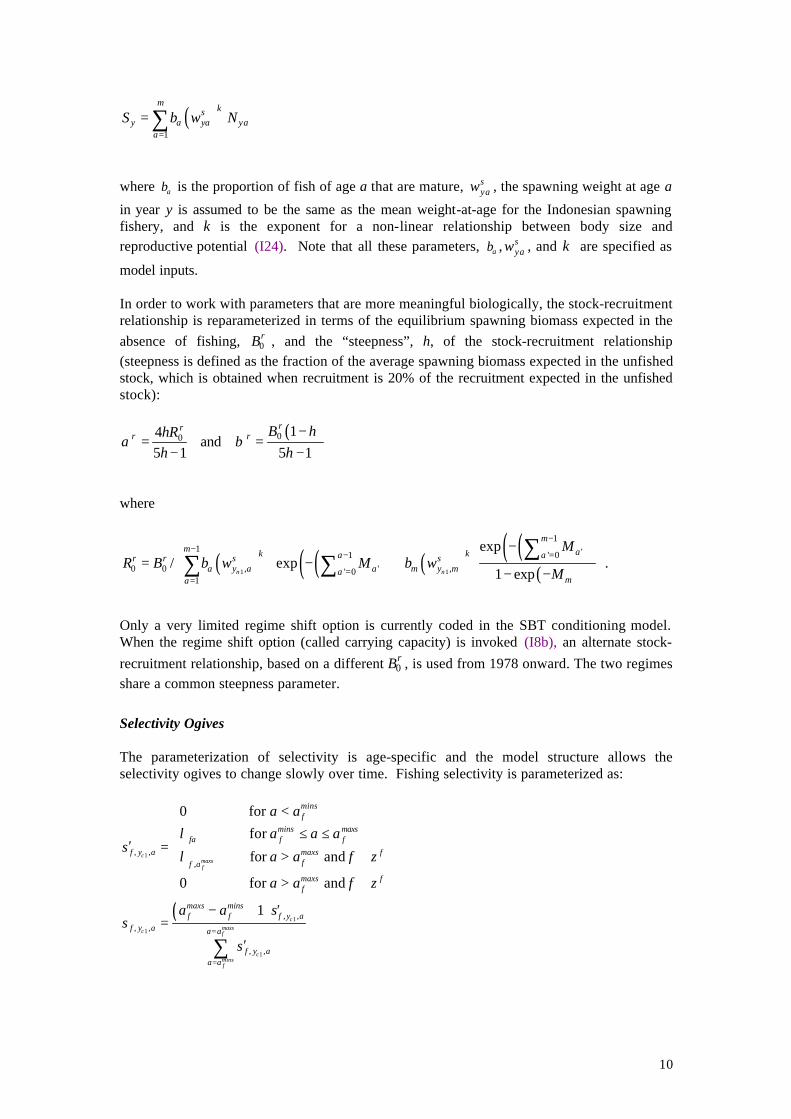
Conditioning and Projections Steepness is included as one of the main grid axis, with values 0.385, 0.55, and 0.73.

Recent recruitments

Conditioning The likelihood assumes no autocorrelation except for the last two years. The empirical autocorrelation in the recruitment residuals estimated over the period 1965-1998 is applied from 2001 onward.

Projection Lognormal autocorrelated error is added to initial abundances (numbers at age 0 through 2 in 2004) within the projection code. Let yτ represent the lognormal recruitment deviate in year y and ˆyτ its MPD estimate. The

initial abundances passed from the conditioning code correspond to 1) 2001τ estimated from model fit

2002 2001ˆˆ ˆτ ρτ=

22003 2001ˆˆ ˆτ ρ τ=

32004 2001ˆˆ ˆτ ρ τ=

where ρ is the empirical estimate of autocorrelation based on recruitments for years 1965-1998. 2) Stochastic projections { }2004,4 2004,4

ˆ exp 0.4 0.08N N z= −

{ }2004,3 2004,3ˆ exp 0.4 0.08N N z= −

{ }2004,2 2004,2 2002ˆ expN N ε=

{ }2004,1 2004,1 2002 2003ˆ ˆexpN N ρ ε ε= +

{ }22004,0 2004,0 2002 2003 2004

ˆ ˆ ˆexpN N ρ ε ρ ε ε= + +

where ( )~ 0,1z N and ( )2 2~ 0,(1 )y RNε ρ σ−

These equations imply that: 2

2004 2004 2002 2003 2004ˆ ˆˆτ τ ρ ε ρ ε ε= + + + which is used to generate

2005 2004 2005ˆτ ρτ ε= + and so on. This formulation amounts to assuming autocorrelated recruitment starting in 2002.

23

Treatment of Rσ

Conditioning Initially Rσ was estimated with a lower bound of 0.40. Since the SAG of 2003, the value has been fixed at 0.6. This was originally done to help achieve a close-to-uniform MCMC distribution of h values within each bin.

Projections Use value passed from conditioning.

Trends in carrying capacity

Conditioning A suggestion was made that one reason many assessments show a low value of steepness may be attributed to changes in carrying capacity. It was suggested that the Aleutian low (i.e., large-scale climate/oceanographic regime shifts) may affect spawning grounds for SBT (but in a way that is not directly obvious). The shift was identified in 1977 and the suggestion was made to apply a different value for R0 (stock-recruitment scale parameter), which would be estimated in the model-fitting process. Results of this conditioning trial resulted in an estimate of h=0.57 and a value of R0 about half the value estimated for the earlier years. The workshop decided to maintain this run as a robustness test. Parameter values related to MSY, depletion, etc. will be computed using the set of parameters estimated for the most recent period.

Projections Use stock recruitment parameters estimated for the most recent period and values of ρ and

Rσ as specified for the baseline sets.

CPUE-abundance relationship

Catchability Model

Conditioning The following model was proposed at the 7th SC meeting to link abundance with expected CPUE.

y

yLLy

ayaajaj jyLL

ayLLy

yyyyy

CPUE

CE

Ns

aa

sN

E

EE

E

EENqCPUE

,1

,

,,112

,,1

2

2000

2000

2000

2000

and

)1(1

~where

1~

2

1

=

+−

=

−+

−+=

∑∑ =

=

ψ

γβϖ

(1)

In this model, parameters 21 andand,,,, aaq yψϖγβ are specified by the user. Current default

values are: .30,4,1,1,0,0 21 ====== aaψωγβ

24

Parameters β and γ : changing the values of β and γ had little or no effect in the conditioning (CCSBT-MP/0304/07). Parameter ω : Is one of the axes in the grid, with values 1 and 0.75. Parameters a1 and a2 (age range to standardize selectivity for CPUE predictions) are included as one grid axes with two alternative ranges: (1) a1=4 and a2=18 (2) a1=8 and a2=12. The rational for changing a2 from 30 to 18 was that selectivities estimated for ages 19-30 are very low.

Projections Same as in conditioning. Trends in efficiency

Conditioning The analyses looking at historical CPUE trend based on a linear increase (CCSBT-MP/0304/07) showed that no improvement was obtained by imposing this relationship. The CPUE working group recommended to include a test assuming a linear increase in catchability of 1% per year throughout the whole time series. This test was later dropped but an increase in q of 0.5 % a year (half way between Q0 and Q1) was kept in both the conditioning and in the projections in the core set. Suggestions were made that catchability might best be modeled as a break-point (two periods, pre and post GPS/plotting). This was supported somewhat with the residual pattern.

Projections The 0.5% annual increase in q is also applied in conditioning. CPUE is generated using autocorrelated trends in catchability, as estimated from conditioning. The empirical estimate of autocorrelation based on the entire time series (1969-2003) is used. For the sigma: use a value of 0.2 or the empirical estimate for the entire time series, whichever is largest. Alternatively, the user can select a value as a command option to the projection code by typing

-cpuestd xx where for xx>=0, the value xx is the standard deviation of the log of the cpue residuals. A sensitivity test assuming a 20% up and down change in q in year 2006 is included. NB!: first int in *.grid file needs to be set by hand to 1 (20% increase in q) or –1 (20% decrease in q) instead of the default 0.

Growth

Projections: Size and weight at age assumed constant over time but different for the four fisheries. Data are input in fixed_quants04.

Errors in catches

Conditioning: Core set assumes no errors in catches. A robustness test is done with actual catches (5% for 1969-1990 and 15% for y≥1991) larger than those in the input file (controlled by a switch in *.dat file).

Projections: - Core set assumes TAC=catch. - When underreporting of catches is assumed in the conditioning, it is also assumed in

projections (actual catch is 15% larger than TAC). Only reported catches are assumed

25

known by the MPs. In other words, the MP does not know the “true” historical catch vectors used for conditioning and the simulated actual catches.