Introduction

1

Panel Data Analysis

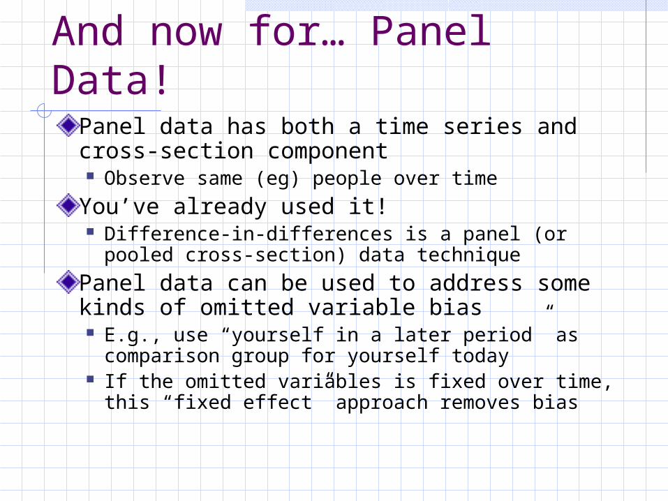
And now for… Panel Data!Panel data has both a time series and cross-section component Observe same (eg) people over time

You’ve already used it! Difference-in-differences is a panel (or pooled cross-

section) data technique

Panel data can be used to address some kinds of omitted variable bias E.g., use “yourself in a later period” as comparison

group for yourself today If the omitted variables is fixed over time, this “fixed

effect” approach removes bias

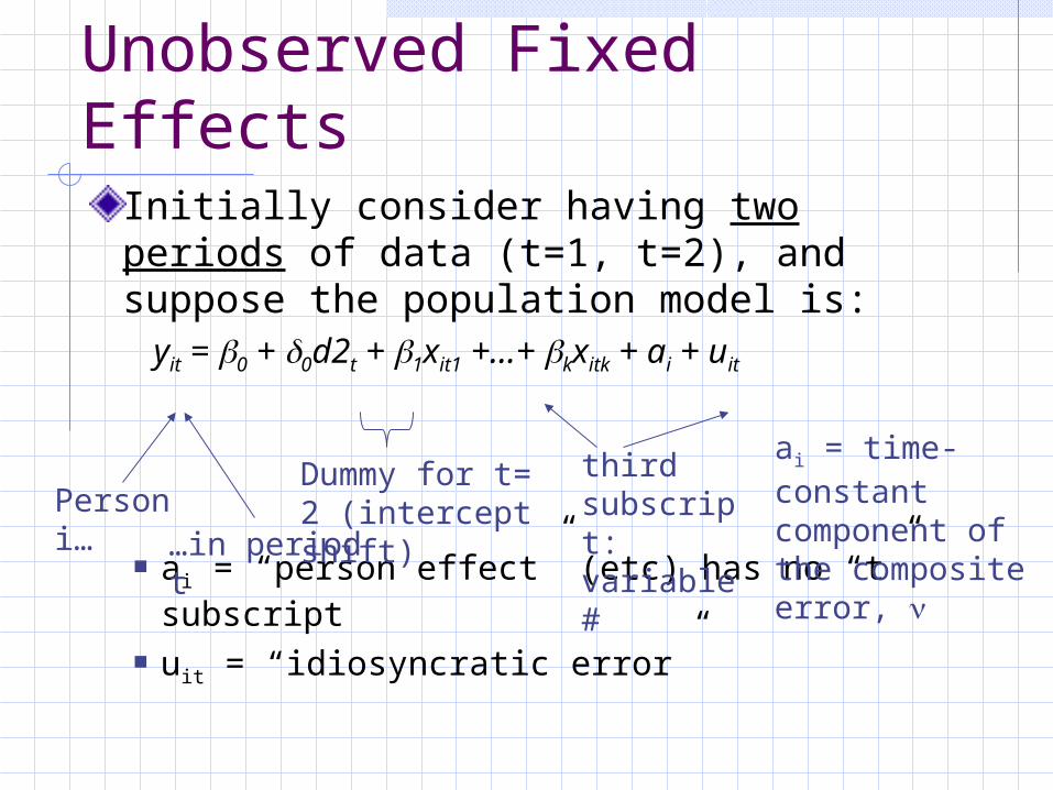
Unobserved Fixed EffectsInitially consider having two periods of data (t=1, t=2), and suppose the population model is: yit = 0 + 0d2t + 1xit1 +…+ kxitk + ai + uit

ai = “person effect” (etc) has no “t” subscript

uit = “idiosyncratic error”

Person i……in period t

Dummy for t= 2 (intercept shift)

ai = time-constant component of the composite error,

third subscript: variable #

Unobserved Fixed EffectsThe population model is yit = 0 + 0d2t + 1xit1 +…+ kxitk + ai + uit

If ai is correlated with the x’s, OLS will be biased, since ai is part of the composite error term

Aside: this also suffers from autocorrelation Cov(i1, i2) = cov(ai,ai) + 2cov(uit,ai) + cov(ui2,ui1)

= var(ai)

So OLS standard errors biased (downward) – more later.

But supposing the uit are not correlated with the x’s – just the fixed part of the error is -- we can “difference out” the unobserved fixed effect…

it

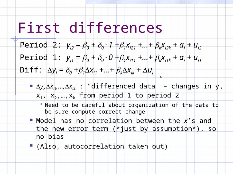
First differencesPeriod 2: yi2 = 0 + 0∙1 +1xi21 +…+ kxi2k + ai + ui2

Period 1: yi1 = 0 + 0∙0 +1xi11 +…+ kxi1k + ai + ui1

Diff: yi = 0 +1xi1 +…+ kxik + ui

yi,xi1,…,xik : “differenced data” – changes in y, x1, x2,…,xk from period 1 to period 2 Need to be careful about organization of the data to be sure

compute correct change Model has no correlation between the x’s and the new

error term (*just by assumption*), so no bias (Also, autocorrelation taken out)

Differencing w/ Multiple Periods

Can extend this method to more periods Simply difference all adjacent periods So if 3 periods, then subtract period 1 from period 2,

period 2 from period 3 and have 2 observations per individual; etc. Also: include dummies for each period, so called “period

dummies” or “period effects”

Assuming the uit are uncorrelated over time (and with x’s) can estimate by OLS Otherwise, autocorrelation (and ov bias) remain

7

Two-period example from textbook

Does higher unemployment rate raise crime? Data from:

46 U.S. cities (cross-sectional unit “i”) in 1982, 1987 (the two years, “t”)

Regress crmrte (crimes per 1000 population) on unem (unemployment rate) and a dummy for 1987

First, let’s see the data…

8

crmrte unem d87

73.31342 14.9 0

63.69899 7.7 1

169.3155 9.1 0

164.4824 2.4 1

96.08725 11.3 0

120.0292 3.9 1

116.3118 5.3 0

169.4747 4.6 1

70.77671 6.9 0

72.51898 6.2 1

… … …

9

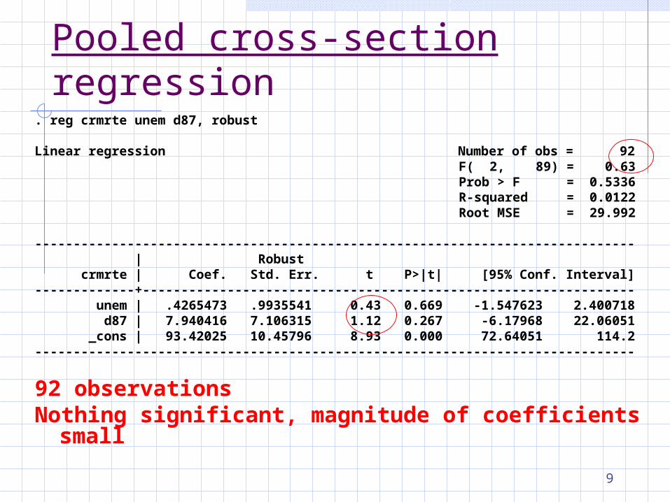
Pooled cross-section regression. reg crmrte unem d87, robust

Linear regression Number of obs = 92 F( 2, 89) = 0.63 Prob > F = 0.5336 R-squared = 0.0122 Root MSE = 29.992

------------------------------------------------------------------------------ | Robust crmrte | Coef. Std. Err. t P>|t| [95% Conf. Interval]-------------+---------------------------------------------------------------- unem | .4265473 .9935541 0.43 0.669 -1.547623 2.400718 d87 | 7.940416 7.106315 1.12 0.267 -6.17968 22.06051 _cons | 93.42025 10.45796 8.93 0.000 72.64051 114.2------------------------------------------------------------------------------

92 observationsNothing significant, magnitude of coefficients small

10

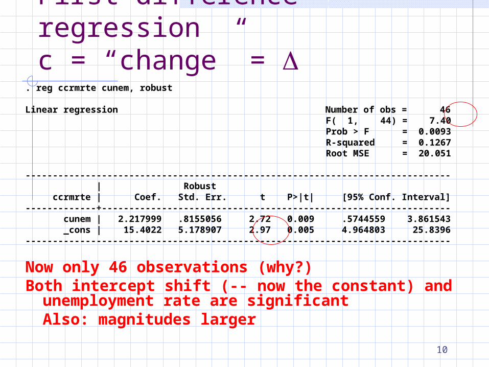
First difference regressionc = “change” =

. reg ccrmrte cunem, robust

Linear regression Number of obs = 46 F( 1, 44) = 7.40 Prob > F = 0.0093 R-squared = 0.1267 Root MSE = 20.051

------------------------------------------------------------------------------ | Robust ccrmrte | Coef. Std. Err. t P>|t| [95% Conf. Interval]-------------+---------------------------------------------------------------- cunem | 2.217999 .8155056 2.72 0.009 .5744559 3.861543 _cons | 15.4022 5.178907 2.97 0.005 4.964803 25.8396------------------------------------------------------------------------------

Now only 46 observations (why?)Both intercept shift (-- now the constant) and

unemployment rate are significantAlso: magnitudes larger

11

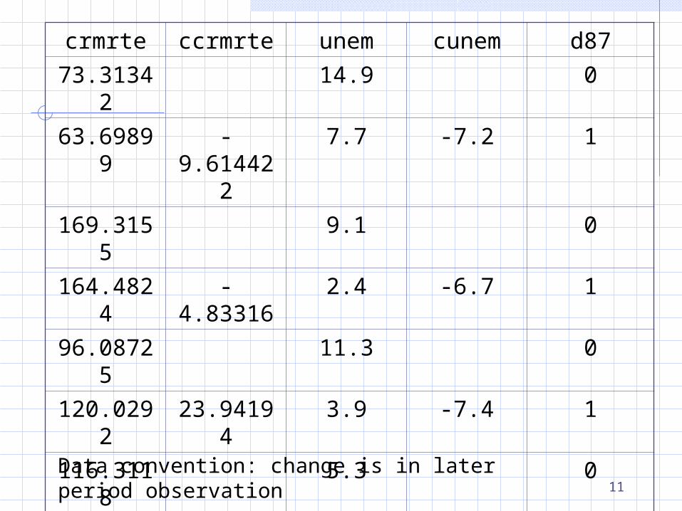
crmrte ccrmrte unem cunem d87

73.31342 14.9 0

63.69899 -9.614422 7.7 -7.2 1

169.3155 9.1 0

164.4824 -4.83316 2.4 -6.7 1

96.08725 11.3 0

120.0292 23.94194 3.9 -7.4 1

116.3118 5.3 0

169.4747 53.16296 4.6 -.7000003 1

70.77671 6.9 0

72.51898 1.742271 6.2 -.7000003 1

… … … … …

Data convention: change is in later period observation

12

Why did coefficient estimates get larger and more significant?

Perhaps cross-section regression suffered from omitted variables bias [cov(xit,ai) ≠ 0] Third factors, fixed across the two periods, which

raise unemployment rate and lower crime rate (??) More generous unemployment benefits? …

To be clear: taking differences can make omitted variables bias worse in some cases To oversimplify, depends which is larger:

cov(xit, uit) or cov(xit,ai)

Possible example: crime and police

13

More police cause more crime?!(lpolpc = log police per capita)

. reg crmrte lpolpc d87, robust

Linear regression Number of obs = 92 F( 2, 89) = 9.72 Prob > F = 0.0002 R-squared = 0.1536 Root MSE = 27.762

------------------------------------------------------------------------------ | Robust crmrte | Coef. Std. Err. t P>|t| [95% Conf. Interval]-------------+---------------------------------------------------------------- lpolpc | 41.09728 9.527411 4.31 0.000 22.16652 60.02805 d87 | 5.066153 5.78541 0.88 0.384 -6.429332 16.56164 _cons | 66.44041 7.324693 9.07 0.000 51.8864 80.99442------------------------------------------------------------------------------

A 100% increase in police officers per capita associated with 41 more crimes per 1,000 populationSeems unlikely to be causal! (What’s going on?!)

14

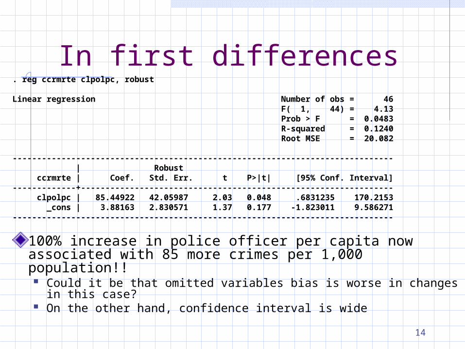
In first differences. reg ccrmrte clpolpc, robust

Linear regression Number of obs = 46 F( 1, 44) = 4.13 Prob > F = 0.0483 R-squared = 0.1240 Root MSE = 20.082

------------------------------------------------------------------------------ | Robust ccrmrte | Coef. Std. Err. t P>|t| [95% Conf. Interval]-------------+---------------------------------------------------------------- clpolpc | 85.44922 42.05987 2.03 0.048 .6831235 170.2153 _cons | 3.88163 2.830571 1.37 0.177 -1.823011 9.586271------------------------------------------------------------------------------

100% increase in police officer per capita now associated with 85 more crimes per 1,000 population!!

Could it be that omitted variables bias is worse in changes in this case? On the other hand, confidence interval is wide

Bottom line

Estimating in “differences” is not a panacea Though we usually trust this variation more

than cross-sectional variation, it is not always the case it suffers from less bias Another example: differencing also exacerbates

bias from measurement error (soon!) Instead, as usual, a credible “natural

experiment” is always what is really critical

15