Intro to Business & Technology 1

Excel Project 3 – What-If Analysis, Charting, and Working with Large Worksheets

*You must use Excel Online to complete this assignment. Go to portal.office.com and log-in to

access Excel Online. *Do NOT use Google Sheets. No credit can be earned if Google Sheets are used. *No credit can be earned if you do not have formulas, so follow directions carefully and closely.

1. Open a blank Excel spreadsheet

2. Save the spreadsheet as Excel Project 3 Modern Music Shops

3. Select cell A8 and then type Modern Music Shops as the worksheet title

4. Select cell A9 and then type Six-Month Financial Projection as the worksheet subtitle

and then press the Enter key

5. In cell B10 type July and then click the Enter box.

6. Be sure cell B10 is still selected, and then click the Alignment Settings button to open the

dialog box. See image below to help you. **If Excel Online does not have this feature,

skip to step 10.

7. The Alignment Settings dialog box should open.

Intro to Business & Technology 2

8. Change the orientation (far right of the dialog box) to 45 degrees. See the image on the next

page to help you.

10. Use your fill handle to copy the remaining months (August through December) to the

range C10:G10. Your spreadsheet should then look like the image below. Save

changes.

9. Save your changes (CTRL + S)

Intro to Business & Technology 3

11. Increase the width of column A to 36.00 (331 pixels). See the image below to help

you.

12. In cell H10, type the word Total. In cell I10, type the word Chart. Format these

cells so that the text is at a 45-degree angle.

Intro to Business & Technology 4 13. Use the image below to type in the row titles for the column A. For the titles that are

indented, use your increase indent button on the Home tab.

14. In cell A1, type What-If Assumptions

15. In the range A2:A6, you will copy and paste the information from the range A16:A20.

See the image on the next page.

Intro to Business & Technology 5

16. If your spreadsheet matches

the image to the left, save changes.

17. Right click on Row 4.

Choose Insert from the Menu. In the

new row you just inserted, type

Margin

18. Right click on Row 7.

Choose Insert from the Menu. In the

new row you just inserted, type Sales

Revenue for Bonus

19. Check your spreadsheet with

the image on the next page, then save

changes.

Intro to Business & Technology 6

20. Select cell B13 and enter 3113612.16 in cell B13, 7962235.53 in cell C13,

5112268.58 in cell D13, 2924627.87 in cell E13, 7630534.65 in cell F13,

and

3424270.23 in cell G13.

21. Use AUTOSUM to find the total for row 13. The total should appear in cell H13.

Save changes.

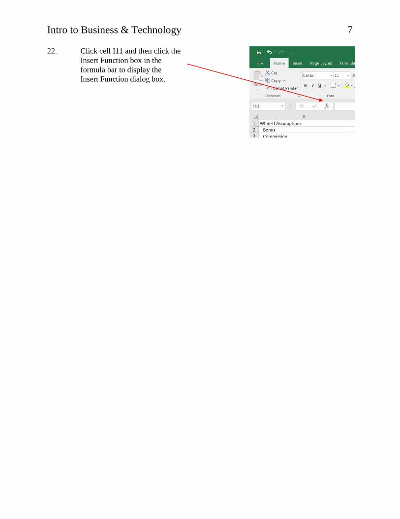
Intro to Business & Technology 7 22. Click cell I11 and then click the

Insert Function box in the

formula bar to display the

Insert Function dialog box.

Intro to Business & Technology 8 23. When the Insert Function dialog box opens, choose Date & Time from the Or select

a category: drop down menu.

24. Scroll down in the list and choose Now. Click OK. Click OK if you get Functional

Argument box.

25. Right on cell I11. Choose Format Cells from the menu. Then click Date. Then

choose the option in the list that says 3/14/12. Click OK. Save changes.

26. In the What-If Assumptions area of the spreadsheet, enter the following values for

each assumption:

Intro to Business & Technology 9 27. Save changes.

28. In cell B14, you will enter a formula with an absolute cell reference. An absolute cell

reference is a cell reference in a spreadsheet that remains constant even if the

spreadsheet shape or size changes, or the reference is copied or moved to another cell

or sheet. The formula for B14 is =B13*(1-$B$4)

The dollar signs in the formula above let you know that B4 is the absolute cell reference.

29. In cell B15, type =B13-B14

30. In cell B18, you will enter an IF function. An IF function is useful when you want to

assign a value to a cell based on a logical test. In cell B18, enter

=IF(B13>=$B$7,$B$2,0)

31. In cell B19, type =B13*B3 then press the F4 key on your keyboard. The F4 key will

automatically change B3 to B$3$, an absolute cell reference. Press Enter.

32. In cell B20, type =B13*B5 then press F4. Press Enter.

33. In cell B21, type =B13*B6 then press F4. Press Enter.

34. In cell B22, type =B13*B8 then press F4. Press Enter.

35. In cell B23, use AUTOSUM to find the total for Total Expenses.

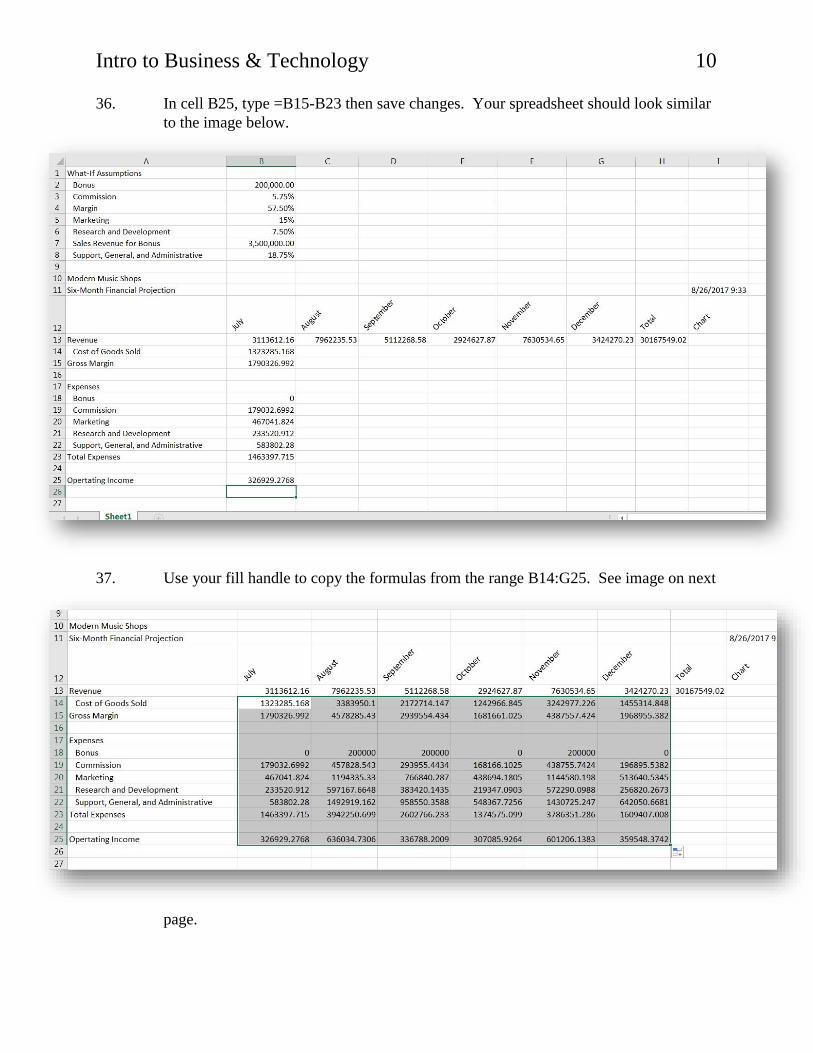
Intro to Business & Technology 10 36. In cell B25, type =B15-B23 then save changes. Your spreadsheet should look similar

to the image below.

37. Use your fill handle to copy the formulas from the range B14:G25. See image on next

page.

Intro to Business & Technology 11 38. Save your changes.

39. Select cell H13 and use your fill handle to copy the formula to H14:H15.

40. Select cell H18 and use AUTOSUM to find the total for row 18. Copy the formula to

the range H19:H23.

41. Select cell H25 and use AUTOSUM to find the total for row 25. Save changes. See

image below if needed.

42. Right click on Sheet 1 tab, click rename, and then type Six-Month Financial

Projection and then press Enter. Right click on Six-Month Financial Projection tab,

click Tab Color and choose purple. Save changes.

43. Be sure the Six-Month Financial Projection spreadsheet is displayed. You will know

format the spreadsheet different fonts, colors, and sizes.

44. Select cell A10. Change the font size to 36.

45. Select cell A11. Change the font size to 18.

Intro to Business & Technology 12

46. Press CTRL + Home to select cell A1

47. Change the font to size 8, italics, and underline

48. Select the range A2:B8, and change the font to size 8.

49. Select the range A1:B8 and then click the Fill Color button and choose purple. Then

change the font color to white.

50. Select the range A10:I11. Change the Fill Color to purple. Change the font color to

white.

51. Select cell A13, Change the Fill Color to purple. Change the font color to white and

bold. Format cell A15 the same way.

52. Select the range A25:H25. Change the Fill Color to purple. Change the font color to

white and bold.

53. Select the range B13:H13. On the Number area of the Home ribbon, change General

to Currency to apply Currency formatting to the selected row.

54. Select the range B15:H15. On the Number area of the Home ribbon, change General

to Currency to apply Currency formatting to the selected row.

55. Select the range B23:H23. On the Number area of the Home ribbon, change General

to Currency to apply Currency formatting to the selected row.

56. Select the range B25:H25. On the Number area of the Home ribbon, change

General to Currency to apply Currency formatting to the selected row.

57. Select the range A12:I12 and choose Heading 3 from the Styles menu list on the

Home tab.

Intro to Business & Technology 13 58. Select the range B15:I15. Apply the Total style from the Styles menu list on the

Home tab. Select the range A23:I23. Apply the Total style from the Styles menu list

on the Home tab.

59. Save changes. Check the next page to be sure your spreadsheet looks like the image

shown.

SCROLL DOWN

Intro to Business & Technology 14

Intro to Business & Technology 15

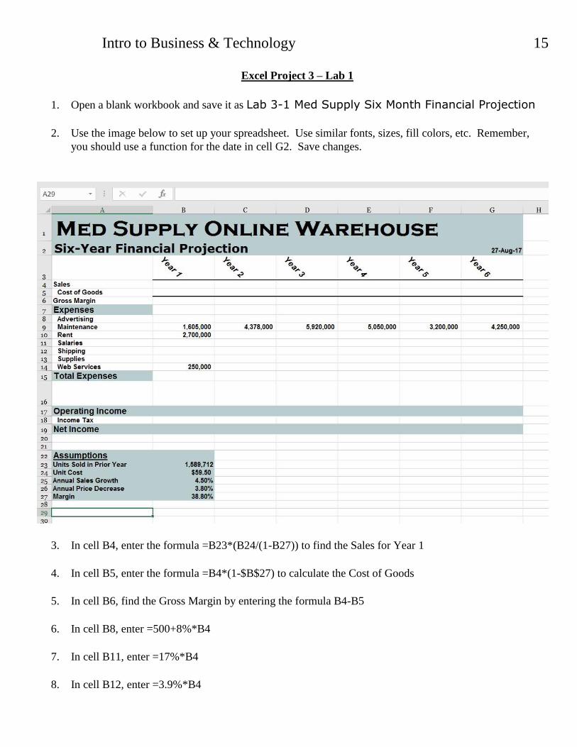
Excel Project 3 – Lab 1

1. Open a blank workbook and save it as Lab 3-1 Med Supply Six Month Financial Projection

2. Use the image below to set up your spreadsheet. Use similar fonts, sizes, fill colors, etc. Remember,

you should use a function for the date in cell G2. Save changes.

3. In cell B4, enter the formula =B23*(B24/(1-B27)) to find the Sales for Year 1

4. In cell B5, enter the formula =B4*(1-$B$27) to calculate the Cost of Goods

5. In cell B6, find the Gross Margin by entering the formula B4-B5

6. In cell B8, enter =500+8%*B4

7. In cell B11, enter =17%*B4

8. In cell B12, enter =3.9%*B4

Intro to Business & Technology 16

9. In cell B13, enter +1.3%*B4

10. In cell B15, use AUTOSUM to find the total of the range B8:B14

11. In cell B17, enter =B6-B15 to find the operating income

12. In cell B18, use an IF Function for the Income Tax. Enter the formula =IF(B17<0,0,45%*B17)

13. In cell B19, find the net income by entering the formula =B17-B18. Save changes.

14. In cell C4, enter the formula =B4*(1+$B$25)*(1-$B$26) to find the Sales for Year 2. Notice how this

formula takes into account the cost of goods from Year 1.

15. Be sure cell C4 is selected. Using your Fill Handle, copy the formula to D4:G4

16. Use your Fill Handle to copy the remaining formulas in Column B to Columns D through G.

17. Your finished Spreadsheet should look similar to the image below.

**Note: Ignore the information in Column H