INTRACTABLE STRUCTURAL ISSUES IN DISCRETE EVENT SIMULATION

"INTRACTABLE STRUCTURAL ISSUES INDISCRETE EVENT SIMULATION: SPECIAL CASES

AND HEURISTIC APPROACHES"

by

E. YUCESAN*and

S.H. JACOBSON**94/38/TM

* Associate Professor of Operations Management, at INSEAD, Boulevard de Constance,77305 Fontainebleau Cede; France.

** Department of Industrial & Systems Engineering, Virginia Polytechnic Institute and StateUniversity Blacksburg, VA 24061-0118, USA.

A working paper in the INSEAD Working Paper Series is intended as a means whereby afaculty researcher's thoughts and findings may be communicated to interested readers. Thepaper should be considered preliminary in nature and may require revision.

Printed at INSEAD, Fontainebleau, France

INTRACTABLE STRUCTURAL ISSUES

IN DISCRETE EVENT SIMULATION:

SPECIAL CASES

AND

HEURISTIC APPROACHES

Enver YucesanINSEAD

European Institute of Business AdministrationTechnology Management Area

77305 Fontainebleau CedexFrance

Sheldon H. JacobsonDepartment of Industrial & Systems EngineeringVirginia Polytechnic Institute and State University

Blacksburg, VA 24061-0118U.S.A.

Abstract

Several simulation model building and analysis issues have been studied using a

computational complexity approach More specifically, four problems related to

simulation model building and analvSis (accessibility of states, ordering of events,

interchangeability of model implementations, and execution stalling) have been shown

to be NP-hard search problems. These results imply that it is unlikely that a

polynomial-time algorithm can be devised to verify structural properties of discrete

event simulation models, unless P = NP. Heuristic procedures should therefore be

useful to practitioners. This paper identifies limited special cases of one of these

problems which are polynomially solvable and NP-hard, and discusses the implications

with respect to the other three problems. A number of heuristic procedures are then

proposed. In particular, four algorithms are presented to address ACCESSIBILITY.

Experimentation with test problems suggests that local optimization approaches such as

simple descent and simulated annealing represent promising approaches for addressing

this structural problem.

Key words - Model validation, verification, local optimization, simulation,algorithms, computational complexity

1. INTRODUCTION

Computer simulation is often described as the most versatile experimental technique in

studying discrete event dynamic systems (DEDS), though it is usually regarded as the

tool of last resort. This reputation is largely due to inherent difficulties in constructing a

correct simulation model. Such difficulties, in turn, are attributed to the lack of a

universally accepted framework for modeling and analyzing DEDS, that is analogous to

the framework of difference or differential equations for depicting continuous variable

dynamic systems (CVDS) [Nance 1981, Balci and Nance 1987, Yucesan 1989, Balmer

and Paul 1990, Ho and Cao 1991].

Over the past two decades, considerable progress has been made in constructing

such a framework [Evans et al. 1967, Zeigler 1976, Overstreet and Nance 1985, Glynn

and Iglehart 1988, Yucesan and Schruben 1993]. In spite of this effort, simulation

modeling and analysis remains a challenging task. In particular, model validation and

verification, an important step in simulation modeling and analysis, is not trivial.

Verification is the process of checking whether a simulation program operates in the

way that the modeller thinks it does, while validation is the process of checking

whether a simulation model, correctly implemented, is a sufficiently close

approximation to the system under study for the intended application [Bratley et al.

1987, p.8].

Although various approaches from software engineering to cognitive modeling

have been proposed, there is no recipe for these tasks. The lack of a set of universally

accepted guidelines contributes to increased testing requirements -hence, costs- as

models with growing complexity are built and maintained [Whitner and Balci 1989].

Problems related to building and analyzing simulation models (such as model

validation and verification) have recently been approached from a computational

complexity perspective [Yucesan and Jacobson 1992]. The theory of NP-completeness

provides a well-defined framework to assess the intractability of decision problems.

Decision problems in the class NP are those problems for which a guessed potential

solution can be verified in polynomial time in the size of the problem instance. The

complete problems in this class (that is, the NP-complete problems) are the hardest

decision problems in NP such that, if one such problem could be solved in polynomial

time, then all problems in NP could be solved in polynomial time [Garey and Johnson

1979]. Moreover, NP-hard problems are search problems which are provably at least

as hard as NP-complete decision problems.

Within this framework, four simulation model building and analysis issues are

cast as search problems: accessibility of states, ordering of events, interchangeability of

model implementations, and execution stalling, and shown to be NP-hard [Jacobson

and Yucesan 1994]. More specifically, a state, S, is said to be accessible, if a finite

sequence of events can be found whose execution leads into S. Two events, A and B,

2

are said to be order-independent, if the execution of event A followed immediately by

event B leads into the same state as the execution of event B followed immediately by

event A, provided that the executions of both AB and BA result in valid event

sequences. Two different computer implementations of a simulation model are called

interchangeable if the same sequence of events executed on the two implementations

always leads to the same state. A simulation model is said to stall if a finite sequence of

events can be found whose execution leads into a state where the termination condition

is not satisfied and the events list is empty.

These results imply that it is highly unlikely that a polynomial-time algorithm

can be devised to verify structural properties of discrete event simulation models,

unless P = NP. In addition to capturing the complexity of a seemingly diverse set of

questions in a unified framework, the consequences of these assertions cover a wide

range of modeling and analysis issues in simulation. These include the detection of rare

events, the specification of a valid experimental frame, the automation of variance

reduction procedures, the verification of the applicability of infinitesimal perturbation

analysis, and the determination of valid stopping conditions for simulation experiments

(for a detailed discussion, see Yucesan and Jacobson [1992]).

Two directions of investigation are possible as a consequence of these results:

(i) the identification of special cases of these problems which are polynomially solvable

or NP-hard; (ii) the application of techniques, that often work in developing heuristics

for NP-hard problems, to these sihiblation problems. This paper pursues these

approaches. In Section 2, preliminary definitions are presented. Special cases that are

polynomially solvable and NP-hard are identified in Section 3. Section 4 introduces

several heuristic procedures, whose performances are assessed in Section 5.

Concluding comments are provided in Section 6. The results here represent a practical

complement to earlier theoretical work [Jacobson and Yucesan 1994].

2. DEFINITIONS

For completeness, the concepts associated with the intractability results are defined.

Some of the definitions are based on the developments in Overstreet [1982] and

Schruben [1992].

From a functional point of view, a system can be viewed as a collection of

entities that interact with a common purpose according to sets of laws and policies. The

state of a system is a complete description of the system. A description of the state of a

discrete event system includes values for all of its numerical attributes as well as any

schedule it may have for the future. Events induce changes in the state of the system.

There are a countable number of event types.

A model is simply a system used as a surrogate for another system. A model

specification is a representation of the system under study, reflecting the objectives of

3

the study and the assumptions of the analysis. A model implementation, on the other

hand, describes a procedure to mimic the system behavior. In other words, a model

specification.defines what a model does while a model implementation defines how the

model behavior is to be achieved. A model specification can be in the form of a

Generalized Semi-Markov Process (GSMP) [Glynn and Iglehart 1988] or an Event

Graph Model (EGM) [Yucesan and Schruben 1993] while a model implementation can

be in a high-level programming language such as Pascal or C, or in a simulation

language such as SLAM [Pritsker 1986] or SIMAN [Pegden et al. 1990]. The EGM

framework will be used in the rest of the paper to define a model specification.

The elements of a discrete event simulation model specification are state

variables that describe the state of the system, events that alter the values of state

variables, and the relationships between events. An event graph is a structure of these

elements in a discrete event system that facilitates the development of a correct

simulation model specification. Hence, the emphasis is directly on system events;

system entities are represented implicitly.

Events are represented on the graph as vertices. Each vertex is associated with

a set of changes to state variables. These variables are used to describe system entities.

Relationships between events are represented in an event graph as directed

edges between pairs of vertices. Each edge is associated with sets of logical and

temporal expressions. Two types of edges are identified. Scheduling edges appear as

solid arcs in the graph whereas cancelting edges are depicted as dashed arcs. The edges

define under what conditions and after how long a time delay one event will schedule or

cancel another event. There can be multiple edges between any pair of vertices; the

edges can point in either direction or may simply point from an edge to itself.

In an event graph, it is also possible to parameterize the event vertices. Event

parameterization is a modeling convenience and does not augment the modeling

capabilities of these graphs. Parameters simply keep the graphs from becoming

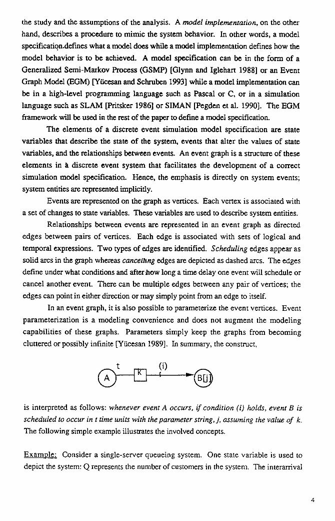
cluttered or possibly infinite [Yiicesan 1989]. In summary, the construct,

is interpreted as follows: whenever event A occurs, if condition (i) holds, event B is

scheduled to occur in t time units with the parameter string, j, assuming the value of k.

The following simple example illustrates the involved concepts.

Example: Consider a single-server queueing system. One state variable is used to

depict the system: Q represents the number of customers in the system. The interarrival

4

and service times are denoted by to and ts, respectively. Three events are used to

capture the dynamic behavior of the system. I is the initialization event where the initial

conditions (empty) of the queueing system are set. A represents a customer arrival

while E represents the end of customer service. The event graph is presented in Figure

1. The state changes associated with an event are shown in brackets next to that event

vertex. The edge conditions are presented in parentheses.

More specifically, an Event Graph is defined as an ordered quadruple

G = (V(G), Es(G), Ec(G), )

where V(G) is the set of vertices of G, Es(G) is the set of scheduling edges of G,

Ec(G) is the set of cancelling edges of G, and 'PG is the incidence function describing

the graph. The entities in this network are then defined as the following ordered sets:F = { fv : v E V(G) ), the set of state transition functions associated with event vertex

v,

C = (Ce : e E Es(G) U Ec(G) ), the set of edge conditions,

T = { to : e E Es(G) ), the set of edge delay times,

r = (-ye : e E Es(G) ), the set of event execution priorities. The execution priority, ye,

is an expression associated with a scheduling edge that computes an execution priority

for the event vertex being scheduled. The Ye are used to break time ties among those

events that are scheduled to occur at the same simulated instance; smaller values

correspond to higher priorities.

5

The key concept is that an event graph specifies the relationships among the

elements of the sets of entities in a simulation model. An Event Graph Model (EGM) isdefined as, (}', C, ?, F, G ) [Yucesan and Schruben 1993]. The first four sets in this

five-tuple define the entities in a model. The role played by the event graph, G , in thedefinition of an EGM is analogous to the role of the incidence function, 'PG , in the

definition of a directed graph; it organizes these sets of entities into a meaningful

simulation model specification. That is, G defines the relationships between elements

in the sets r, C , T, and F. Note that an EGM is just a Generalized Semi-Markov

Scheme (GSMS) [Glasserman and Yao 1992]. The specification of an appropriate

measure for? yields a Generalized Semi-Markov Process (GSMP).

The EGM formalism focuses on model specifications for DEDS. The objective

is to have a static picture of the underlying structure rather than to describe possible

sample paths. This formalism enables model implementations to be obtained directly

from model specifications without requiring any additional transformations. In fact, an

EGM can be implemented using a high level programming language or a general

purpose simulation language by possibly coding subgraphs into separate event routines

[Som and Sargent 1989]. A direct implementation is also possible using the software

package SIGMA [Schruben 1992].

3. SPECIAL CASES

3.1 Search Problems

The search problems, ACCESSIBILITY, ORDERING, INTERCHANGEABILITY,

and STALLING are formally defined in Jacobson and Yucesan [1994]. For

completeness, these problems are stated below.

ACCESSIBILITYInstance: A discrete event simulation model specification,

An initial event, E.°,

A state, S,

A non-negative finite integer, M.Ouestion: Find a sequence of events El, E2, Em, m M, such that

the execution of the sequence yieldsEoE1E2...Em S

ORDERINGInstance: A discrete event simulation model specification,

An initial event, Eso,

Two distinct states, S 1 and S2,

A non-negative, finite integer, K.

6

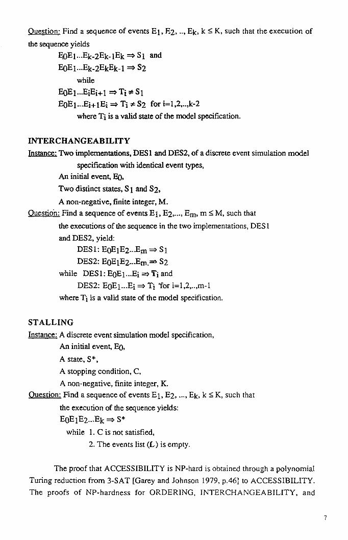
Ouestion: Find a sequence of events El, E2, Ek, k K, such that the execution of

the sequence yieldsEoE ...Ek_2Ek_iEk S1 and

E0E1...Ek_2EkEk_1 S2

while

SiE0E1...Ei-F iEi Ti � S2 for i=1,2,..,k-2

where Ti is a valid state of the model specification.

INTERCHANGEABILITY

Instance: Two implementations, DES 1 and DES2, of a discrete event simulation model

specification with identical event types,

An initial event, E.°,

Two distinct states, SI and S2,

A non-negative, finite integer, M.

Ouestion: Find a sequence of events El, E2,..., Em, m 5 M, such that

the executions of the sequence in the two implementations, DES 1

and DES2, yield:

DES1: E.OE1E2.--Em SIDES2: EoEIE2...Em.=5 S2

while DES 1: EoEi...Ei Ti and

DES2: EoEi...Ei Ti 'for i=1,2,..,m-1

where Ti is a valid state of the model specification.

STALLINGInstance: A discrete event simulation model specification,

An initial event, Eo,

A state, S*,

A stopping condition, C,

A non-negative, finite integer, K.

Question: Find a sequence of events Ei, E2, Ek, k K, such that

the execution of the sequence yields:

EgiE2...Ek S*

while 1. C is not satisfied,

2. The events list (L) is empty.

The proof that ACCESSIBILITY is NP-hard is obtained through a polynomial

Turing reduction from 3-SAT [Garey and Johnson 1979, p.46] to ACCESSIBILITY.

The proofs of NP-hardness for ORDERING, INTERCHANGEABILITY, and

7

STALLING can all be traced back to ACCESSIBILITY. Therefore, any special cases

of ACCESSIBILITY that are NP-hard will also be NP-hard for the other three

problems.

3.2 Restrictions

The statement of the instance for ACCESSIBILITY indicates that meaningful

restrictions can only be placed on the discrete event model specification, hence, on how

state changes occur. Trivial special cases of the initialization event, EO, (e.g., EO

immediately establishes the desired state S) or the length of the event sequence, M

(e.g., M = 0) are not considered.

Consider first a discrete event simulation model specification with events

defined such that the value of the state monotonically increases by unity from the initial

state, Se, for all events. An example of such a specification would be a Poisson arrival

process -or, more generally, pure birth processes- where the state corresponds to the

number of arrivals -or births- within a given observation window. Clearly, executing

S-SO arrival events results in a solution to this special case of ACCESSIBILITY. In

particular, if 0 S-Se M, the solution to ACCESSIBILITY is a sequence of arrival

events, while if S-Se < 0 or S-S0 > M, the answer to ACCESSIBILITY cannot be

found. Therefore, this special case is solvable in polynomial time in the size of the

problem instance. Note that, if the unit state changes can be either negative or positive

(e.g., a birth-and-death process), than the problem remains polynomially solvable.

Such systems are sometimes referred togas skip-free processes. The associated special

cases of ORDERING, INTERCHANGEABILITY, and STALLING are also trivially

solvable in polynomial time, using the same solution approach.

If this special case is generalized by allowing each executed event type to result

in a positive increase of arbitrary integer size in the state value, where each event can be

executed only once and all events can schedule any other event not yet scheduled, then

the resulting special case of ACCESSIBILITY is no longer easily solvable. In fact, the

resulting problem is a generalization of the SUBSET SUM decision problem [Garey

and Johnson 1979, p.223], which is NP-complete, though solvable in pseudo-

polynomial time using a dynamic programming formulation. This special case of

ACCESSIBILITY is formally stated.

ACCESSIBILITY WITH POSITIVE INTEGER STATE CHANGES

Instance: A discrete-event simulation model specification with a finite set

of events, V(G), where the execution of event v E V(G) results in a

state change of fv, a non-negative finite integer value, where each event

can be executed at most once, and each event can schedule any other

event not yet scheduled,

8

An initial event, EO,

A state, S e Z+,

A non-negative, finite integer M.Ouestion: Find a sequence of events El, E2, Em, m M,

such that the execution of the sequence yields EOE I E2...Em S.

An example of a system which can be described with this type of model

specification is a Poisson process with batch arrivals, where each batch size can only be

observed a specified number of times. To prove that this search problem is NP-hard, a

polynomial Turing reduction from SUBSET SUM can be constructed. First, SUBSET

SUM is formally stated.

SUBSET SUM

Instance: A finite set of elements A with non-negative integer weights, s(a),

ae A,

A positive integer, B.

Ouestion: Does there exist a subset A' of A, A' C A, such that

aE A' s(a) = B ?

The following theorem proves that ACCESSIBILITY WITH POSITIVE INTEGER

STATE CHANGES is NP-hard.

THEOREM: ACCESSIBILITY WITH POSITIVE INTEGER STATE CHANGES is

NP-hard.

Proof: A polynomial Turing reduction from SUBSET SUM to ACCESSIBILITY

WITH POSITIVE INTEGER STATE CHANGES is constructed. To this end, a

special case of ACCESSIBILITY WITH POSITIVE INTEGER STATE CHANGES

must be constructed for a general instance of SUBSET SUM. Given a general instance

of SUBSET SUM, define ACCESSIBILITY WITH POSITIVE INTEGER STATE

CHANGES as follows: the set V(G) is defined as the set A. Therefore, each element

of A corresponds to an event in the simulation model specification. The state change

associated with each event v E V(G) is fv, the weights for the elements of A in

SUBSET SUM. These state changes are non-negative, by the statement of SUBSET

SUM. All the events in V(G) can schedule any of the other events. However, once an

event is scheduled, it can never be scheduled again. Define the initial event EO to set

the initial state to zero. Define the state S to be B. Define the integer value M to be the

cardinality of A ( i.e., IAI = M).

This reduction is done in linear, hence polynomial, time in the size of the

SUBSET SUM problem instance.

9

Suppose that a sequence of events can be found to solve ACCESSIBILITY

WITH POSITIVE INTEGER STATE CHANGES. Associated with each of these

events is an .element of A for SUBSET SUM. Since the initial state for the simulation

model specification is zero and the state changes are defined as the weights for the

elements in A, the subset of elements of A associated with the sequence of events

which solves ACCESSIBILITY WITH POSITIVE INTEGER STATE CHANGES

also solves SUBSET SUM. q

Considering further special cases does not offer much relief. For example, if

the state changes can be either positive or negative, then the problem remains NP-hard.

A queueing system with batch arrivals and batch processing with random yields, in

which the state of the system is described by the number of customers in the system, is

an example of such a special case. In addition, if the value of M is less than the number

of events, the problem remains NP-hard. Note that since ORDERING,

INTERCHANGEABILITY, and STALLING are all at least as hard as

ACCESSIBILITY, then the special cases listed here for these three problems all remain

NP-hard.

The search problem ORDERING is polynomially solvable, if all the events

produce identical state changes. For this special case, it is trivial to show that no

sequence of events solves ORDER MC; The search problem STALLING, on the other

hand, remains NP-hard, even if the Stopping condition is dropped and the problem is

defined only by the events list becoming empty. This can be seen in the Turing

reduction presented in Jacobson and Yucesan [1994].

Another special case concerns the identification of the state types in a finite-

state, discrete-time Markov chain. With such a model specification, the states can be

classified in polynomial time using the Fox-Landi algorithm [Fox and Landi 1968].

However, if the number of states is countably infinite, then the algorithm is no longer

polynomial.

4. HEURISTIC PROCEDURES

Four heuristic procedures are proposed for the NP-hard search problem

ACCESSIBILITY. These procedures are applied to various simulation models and

their performance, together with various implementation issues, are reported in Section

5.

4.1 Event Tree Heuristic

The enumeration of all possible event sequences has been considered by Evans et al.

[1967]. Suri [1989] uses such a tree to analyze the propagation of a perturbation

10

through different sample paths within the context of infinitesimal perturbation analysis.

This method can be easily adapted in a heuristic procedure for solving

ACCESSIBILITY.

Starting from the initial event, E0, all possible event sequences can be

enumerated using a tree diagram called an event tree. The validity of each event

sequence (defined at each branch) can be verified from the event definitions. This event

tree can be built sequentially (breadth first) until a sequence of events, that achieves the

desired state, S, is identified or all possible sequences of specified length, M, have

been exhausted. In general, if there are e events, then there are at most eM sequences

of M events, with each such sequence corresponding to a branch in the tree. The

following example illustrates the approach.

Example (continued): Consider the single-server queueing model of Figure 1. If the

desired length of the event sequence is M=4 and the state of interest is S=3 (denoting a

system size of 3 customers), then there exist 16 possible event sequences (though not

all are valid). The resulting event tree, depicting only valid event subsequences, is as

follows:

AA

EA

AE

I A E

AE A

This event tree depicts all the possible valid event sequences with zero events (I), with

one event (IA), with two events (IAA, IAE), with three events (IAAA, IAAE, IAEA),

and with four events (IAAAA, IAAAE, IAAEA, IAAEE, IAEAA, IAEAE). Note that

there are 6 valid, hence 10 invalid sequences of four events. With S=3. the solution to

ACCESSIBILITY is given by the event sequence IAAA.

Note that, for the single-server queueing model, excluding the initialization

event, there are 2M possible event sequences of length M. However, not all these

event sequences are valid. It can be shown through an induction argument that there

rM)

exist 41 ) valid event sequences, where t = Ma if M is even and p. = (M-1)/2, if M is

odd. The, exponential explosion of the event tree is formally stated and proven in

Appendix A.

4.2 Dynamic Programming HeuristicSuppose there are r < co states and e < co events for a discrete event simulation model

specification. If r (e) is infinite, then a finite subset of states (events) must be selected.

The dynamic programming heuristic sequentially constructs Mr x r matrices that

indicate whether it is possible to move between the r states for a discrete event

simulation model specification within a certain number of events. This heuristic is

similar in nature to the algorithm presented by Fox and Landi [1968] for identifying the

ergodic subchains and transient states of a stochastic matrix. The procedure is as

follows:

Step 0: Identify the r states (S1, S2, .., Sr), where S E (Si, S2,.., Sr). Note that the initial event, EP, defines the initial state, So E

(Si, S2, .., Sr}.

Step 1: Determine if there exists a single event that takes the system

from state Si to state Sj, ij = 1,2, ..,r. Since there are e events and

r2 pairs of states, then this check can be done in O(er2p(n)), where

p(n) is the time it takes to execute an event and n is the size of the

problem instance encoded on a Turing machine.

For h = 2, ..., M:

Step h: Determine if a sequence of h events exists that takes the

system from state Si to Sj, ij = 1,2, ..,r. This can be done using

the (h-1)st matrix. In particular, using a last-step analysis, there are

e events and r states to be checked for each of the r 2 pairs of states.

Therefore, this can be done in O(er3p(n)).

Step M+1: Check the M matrices to see whether it is possible to

reach state S from state SO. This can be done in O(Mr2).

The total complexity of this dynamic programming heuristic is O(Mer3p(n)).

Note that this heuristic does not produce the required event sequence, but simply

indicates whether such a sequence exists. It is, however, possible to report this

sequence by simply keeping track of the desired events at each step of the algorithm. If

the number of states and the number of events are finite, then this heuristic establishes

in pseudo-polynomial time the existence of a solution to ACCESSIBILITY. If the

12

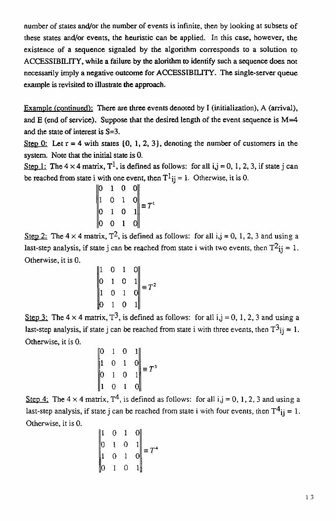
number of states and/or the number of events is infinite, then by looking at subsets of

these states and/or events, the heuristic can be applied. In this case, however, the

existence of a sequence signaled by the algorithm corresponds to a solution to

ACCESSIBILITY, while a failure by the alorithm to identify such a sequence does not

necessarily imply a negative outcome for ACCESSIBILITY. The single-server queue

example is revisited to illustrate the approach.

Example (continued): There are three events denoted by I (initialization), A (arrival),

and E (end of service). Suppose that the desired length of the event sequence is M=4

and the state of interest is S=3.

Step 0: Let r = 4 with states (0, 1, 2, 3), denoting the number of customers in the

system. Note that the initial state is 0.

Step 1: The 4 x 4 matrix, T 1 , is defined as follows: for all ij = 0, 1, 2, 3, if state j can

be reached from state i with one event, then T l ij = 1. Otherwise, it is O.0 1 0 0

1 0 1 0T'

0 1 0 1

0 0 1 0

Step 2: The 4 x 4 matrix, T2, is defined as follows: for all i,j = 0, 1, 2, 3 and using a

last-step analysis, if state j can be reached from state i with two events, then T 2ij = 1.

Otherwise, it is 0.1 0 1 0

0 1 0 1-E. T2

1 0 1 0

0 1 0 1

Step 3: The 4 x 4 matrix, T3 , is defined as follows: for all i,j = 0, 1, 2, 3 and using a

last-step analysis, if state j can be reached from state i with three events, then T 3ij = 1.


1 0 1 0 _T 3

0 1 0 1

1 0 1 0

Step 4: The 4 x 4 matrix, T4, is defined as follows: for all i,j = 0, 1, 2, 3 and using a

last-step analysis, if state j can be reached from state i with four events, then T 4ij = 1.


0 1 0 1

1 0 1 0

0 I 0 1

13

Step 5: A Tr1103 = 1 for m = 1, 2, 3, or 4 signals the existence of an event sequence

that solves ACCESSIBILITY. Otherwise, an answer to ACCESSIBILITY cannot be

given, since .= uncapacitated single-server queue has an infinite number of states. Inthis case, T303 = 1 and the event sequence IAAA solves ACCESSIBILITY.

4.3 Simple Descent

Simple descent (SD) uses local search concepts. Roughly speaking, local search

algorithms start with an initial solution. A neighbor of this solution is then generated

by some suitable mechanism and the change in an associated cost function is calculated.

If a reduction in cost is achieved, then the current solution is replaced with the

generated neighbor. Otherwise, the current solution is retained. The process is

repeated until no further improvement can be found in the neighborhood of the current

solution; the algorithm then terminates at a local minimum. Note that the local

minimum found may be far from the global optimum.

To construct a local search algorithm for solving ACCESSIBILITY, a

configuration space, a neighborhood structure, and an objective function must be

defined. This results in an optimization version of ACCESSIBILITY (called

ACCOPT), where the existence of a configuration space point with an objective

function value of zero indicates that a solution to ACCESSIBILITY can be found. On

the other hand, if all configuration points have nonzero objective function values, then

no such solution to ACCESSIBILITY exists.

To this end, the following definitions are formally introduced. Once again,

suppose that there are e events associated with the simulation model specification. The

configuration space is made up of all possible sequences of M events. There are eM

such sequences, though not all constitute valid event sequences. The neighbors of each

configuration space point are obtained by changing exactly one event in the sequence.

This neighborhood structure will be termed one-change. Therefore, with one-change,

eacliconfiguration space point has M(e-1) neighbors.

The objective function is defined as follows: given the configuration spacepoint EOEI....EM, let EOEI....Ek Sk, k=0, 1, 2, .., M, where Sk is the terminating

state for the event subsequences. If EOE1....Ek is not a valid subsequence of events,

then Sk = ce. Using this convention, an objective function is defined as:

f(E0E ....Em) II Sk - S II,

where II • II is a norm on the state space. This function can be evaluated in O(Mp(n)).

These definitions cast ACCOPT as a combinatorial optimization problem. A

polynomial Turing reduction from ACCESSIBILITY to ACCOPT can be constructed to

establish that the latter is NP-hard. ACCOPT is now formally defined.

14

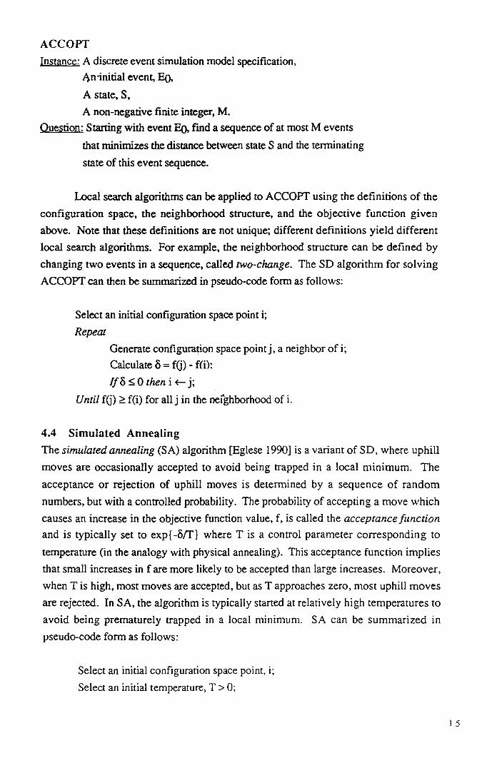
ACCOPT

Instance: A discrete event simulation model specification,

An-initial event, EO,

A state, S,

A non-negative finite integer, M.

Ouestion: Starting with event Eo, find a sequence of at most M events

that minimizes the distance between state S and the terminating

state of this event sequence.

Local search algorithms can be applied to ACCOPT using the definitions of the

configuration space, the neighborhood structure, and the objective function given

above. Note that these definitions are not unique; different definitions yield different

local search algorithms. For example, the neighborhood structure can be defined by

changing two events in a sequence, called two-change. The SD algorithm for solving

ACCOPT can then be summarized in pseudo-code form as follows:

Select an initial configuration space point i;

Repeat

Generate configuration space point j, a neighbor of i;

Calculate 8 = f(j) - f(i):

If 0 then i j;

Until f(j) f(i) for all j in the neighborhood of i.

4.4 Simulated Annealing

The simulated annealing (SA) algorithm [Eglese 1990] is a variant of SD, where uphill

moves are occasionally accepted to avoid being trapped in a local minimum. The

acceptance or rejection of uphill moves is determined by a sequence of random

numbers, but with a controlled probability. The probability of accepting a move which

causes an increase in the objective function value, f, is called the acceptance function

and is typically set to exp{ -8/T } where T is a control parameter corresponding to

temperature (in the analogy with physical annealing). This acceptance function implies

that small increases in f are more likely to be accepted than large increases. Moreover,

when T is high, most moves are accepted, but as T approaches zero, most uphill moves

are rejected. In SA, the algorithm is typically started at relatively high temperatures to

avoid being prematurely trapped in a local minimum. SA can be summarized in

pseudo-code form as follows:

Select an initial configuration space point, i;

Select an initial temperature, T > 0;

15

Set the temperature change coefficient, 0< a <I;

RepeatSet repetition counter, n = 0;

RepeatGenerate configuration space point j, a neighbor of i;

Calculate 8 = f(j) - f(i);

If 8 < 0 then i j;else if random(0,1) < exp( -8/T} then i j;

n n+1;

Until n = N;T aT;

Until stopping criterion true.

The algorithm proceeds by attempting a certain number of neighborhood moves, N, at

each temperature, while T is gradually dropped. The determination of the initial

temperature, the rate at which the temperature is lowered, the number of iterations at

each temperature, and the criterion used for stopping are collectively referred to as the

cooling or annealing schedule. The following example illustrates the definitions used in

local search algorithms.

Example (continued): The three events for the single-server queuein g model are

denoted by I (initialization), A (arrival), and E (end of service). If the desired length of

the event sequence is M=4 and the state of interest is S=3, then there are 16 elements in

the configuration space with associated one-change neighbors and objective function

values, where the objective function is defined using the Li norm. The configuration

space is depicted in Table 1.

A second optimization version of ACCESSIBILITY can be formulated. This

version, called ACCOPT2, tries to find the minimum number of events needed to reach

state S. As for ACCOPT, this problem can be shown to be NP-hard through a Turing

reduction from ACCESSIBILITY.

ACCOPT2

Instance: A discrete event simulation model specification,

An initial event, E0,

A state, S.

Ouestion: Starting with event E0, determine the shortest sequence of

events that reaches state S.

16

Note that solutions to ACCOPT and ACCOPT2 solve ACCESSIBILITY. More

specifically,'if the minimum distance to state S is zero for ACCOPT, then the resulting

event sequence solves ACCESSIBILITY, while, if the distance is greater than zero,

then no such solution exists. Similarly, if the solution to ACCOPT2 has M or fewer

events, then the resulting event sequence solves ACCESSIBILITY, while if the

solution to ACCOPT2 has more than M events, then no such solution exists.

Point No. Elements State(s) Rchd Obj Fnc, f(•) Neighbors

2,3,4,51 IAAAA 0,1,2,3,4 0

2 IAAAE 0,1,2,3,2 0 1,6,7,11

3 IAAEA 0,1,2,1,2 1 1,6,8,10

4 IAEAA 0,1,0,1,2 1 1,7,8,9

5 IEAAA 00 3 1,9,10,11

6 IAAEE 0,1,2,1,0 1 2,3,12,13

7 IAEAE 0,1,0,1,0 2 2,4,12,14

8 IAEEA 0. 2 3,4,12,15

9 IEEAA .... 3 4,5,14,15

10 IEAEA 00 3 3,5,13,15

11 IEAAE 00 3 2,5,13,14

12 IAEEE 00 2 6,7,8,16

13 IEAEE co 3 6,10,11,16

14 IEEAE 00 3 7,9,11,16

15 IEEEA 00 3 8,9,10,16

16 IFFEE .... 3 12,13,14,15

Table 1. The Configuration Space for the Single-Server Queue

The SD and SA algorithms can be applied to ACCOPT2. The configuration

space and neighborhood structures defined for ACCOPT can be used for ACCOPT2 as

well. The objective function for a sequence of events can be defined as

g(E0E1...Er) = R II Sr - S II + r,

where R is a large positive integer such that RII SrS II » M for all event sequences Eo,

El,...,Er that cannot reach state S with M or fewer events. Note that, if state S is

unreachable, then the objective function value is defined to be very large. Therefore,

g(E0E 1...Er) M if and only if state S is reachable with M or fewer events.

Moreover, if g(E0E1...Er) 5 M, then the smallest value this objective function can

assume indicates the minimum number of events that must be executed to reach state S.

17

5. ALGORITHMS FOR ACCESSIBILITY

In this seotiOn, the heuristic approaches proposed for solving ACCESSIBILITY are

described. Details of the implementation of these algorithms are presented.

Experiments with five test problems are discussed.

5.1 Description of the Algorithms

Three algorithms were implemented: event tree heuristic, simple descent algorithm, and

simulated annealing. Furthermore, different variants of the generic SA algorithm were

used to enhance its effectiveness. During preliminary experimentation, it was

discovered that the dynamic programming heuristic suffered from a "state space

explosion" problem as the number of events in a model specification increased.

Therefore, this heuristic has not been pursued any further. The three algorithms are

presented in pseudo-code form.

Event Tree Algorithm:

Initialize variables;

Read data describing the model specification;

Read the required length of event sequence, M;

Read the desired target state

Set counter, m <— 1;

Construct an initial array of all'possible event sequences of length rn;

Do a validity check and return array, of valid event sequences;

If S is reached then exit (report event sequence);

Repeat

Set m f- m+1;

Construct array, 3,-, of all possible new sequences of length m;

Do a validity check and return array, R ., of valid event sequences;

If S is reached then exit (report event sequence);

Until m =M;

Exit (no solution found).

Simple Descent (for ACCOPT):




Read the desired target state, S;

Read the maximum number of iterations, imax;

Set counter, n 0;

Create an initial sequence of events, x, of length M;

Compute the objective function value, f(x);

If f(x) = 0 then exit (report event sequence);

Repeat

Set n n + 1;

Generate a neighborhood array, a[x], of all neighbors of x;

Calculate the objective function value, f(y), for all neighbors y E a[x];

If f(y) = 0 for some y E a[x] then exit (report event sequence);

Else do begin

Calculate 8 = f(y) - f(x);

If 6 > 0 then exit (no solution found);

Else do begin

Create an array of event sequences with the smallest f( •) value;

Pick at random one of these sequences to construct the next

neighborhood;

End;

End;

Until n = imax;


Simulated Annealing (for ACCOPT):




Read the desired target state, S;

Set initial temperature, T > 0;

Set the temperature change coefficient, 0 < a <1;

Set the desired number of temperature changes, iterl;

Set the desired number of iterations at a given temperature, iter2;

Create an initial sequence of events, x, of length M;

Compute the objective function value, f(x);

If f(x) = 0 then exit (report event sequence);

Set the temperature change counter, t 0;

Repeat

Set counter, n 0;

Repeat

Generate another sequence, y, of length M, a neighbor of x;

19

If f(y) = 0 then exit (report event sequence);

Calculate 5 = f(y) - f(x);

If < 0 then x y;

Else if md(0,1) < exp[-5 / 11 then x y;

Endif

n4--n+1;

Until n = iter2;

t<—t+1;

T aT;

Until t = iterl;


5.2 Implementation Issues

The formalism of an EGM is used for the representation of the simulation model

specifications in implementing the above algorithms. Such a representation is required

in computing the objective function value, f •), associated with a generated sequence

for determining a direction to move for the algorithm.

All of the algorithms are implemented in Turbo Pascal on a Compaq 486/33.

This environment was appropriate for testing short sequences of up to 10 events.

Longer sequences, however, necessitated a move to a mainframe computer

(VAX/VMS) due to excessive memory requirements. The event tree algorithm, which

is a complete enumeration scheme, created further run-time problems even on the

mainframe for event sequences of modest length.

Each experimental configuration consisting of a given model and a particular SA

algorithm was replicated twenty times using independently seeded runs. The average

performance indicators (average number of iterations and average run time) are

presented in the subsequent section. Common random numbers are used across

configurations to reduce the variance in the results.

5.3 Test Models

Five test models are used to experiment with the algorithms. The first one is the simple

single-server queue, which was introduced in Section 2. The single-server model is

extended by introducing random breakdowns for the server. This model constitutes

our second test problem. The third test problem is a tandem queue with three stations

and cycle blocking. The description of this model can be found in Onvural and Perros

[1986]; an event graph representation is given in Yiicesan [1989]. In our experiments,

a capacity limit of three is used at all three stations. The Oil Tanker model from Law

and Kelton [1991, p.121] is the fourth test problem. The fifth model is an (s,S)

inventory control policy simulation. Such a system is described in Karlin and Taylor

20

[1975, p.53]. In our experiments, a (s,S) = (4, 10) control policy is used in which

unmet demand is backlogged.

In these experiments, the target states are defined as follows: in the simple

single-server queueing model as well as in its extension with breakdowns, the target

state is expressed as a pre-specified queue length (S=9). In the tandem queue model,

the target state is expressed as a vector of desired queue lengths, S = (n l, n2, n3) =

(1,2,2). The target state in the Oil Tanker problem is a particular value for the number

of tankers waiting to be berthed (S=Q=12). Finally, a particular level of backlog

(inventory position = -7) is taken to be the target state for the inventory management

example.

5.4 Numerical Results

The event tree heuristic requires a large amount of memory, since it is necessary to

maintain arrays of event sequences of length M. This forced the move to a mainframe

computer even for unrealistically short event sequences. The results of our experiments

are summarized in Tables 2a-c. An asterisk (*) implies that the program was aborted

without reporting a result as the memory limits of the computer were reached.

Observe that the algorithm based on complete enumeration of all valid event

sequences is not practical even for fairly short event sequences. For the simple single-

server queueing model, which doesaidtrequire excessive memory, the run time jumps

from 19 seconds for sequences of at most 15 events to over 7 minutes for sequences of

at most 20 events on a mainframe! For slightly more complex models, the memory

requirements quickly overwhelm the capability of the computer.

The same kind of problem was encountered during the pilot experiments with

the dynamic programming heuristic. As the number of states in a model specification

increased, the amount of memory required to store the matrices T m, m=1,2,..,M, grew

substantially, making the heuristic impractical. For this reason, the heuristic was not

pursued any further.

MODEL CPU TIME (sec)

Simple queue 7.55

Simple queue w/ breakdown 35.25

Tandem queue w/ blocking 26.08

Oil Tanker Problem 13.54

(s,S) Inventory policy 6.96

Table 2a. Event Tree Heuristic - Maximum Sequence Length, M = 10


Simple queue 19.53

Simple queue w/ breakdown

Tandem queue w/ blocking *

Oil Tanker Problem *


Table 2b. Event Tree Heuristic- Maximum Sequence Length, M=15


Simple queue 7:19.09

Simple queue w/ breakdown *

Tandem queue w/ blocking *

Oil Tanker Problem *

(s,S) Inventory Policy 9.65

Table 2c. Event Tree Heuristic - Maximum Sequence Length, M=20

For the SD algorithm, the selection of the initial sequence of events has a big

impact on the run time. Starting from a randomly generated initial sequence, which is

not necessarily valid, the algorithm fends to spend a considerable amount of time in

reaching a neighborhood of valid sequences of events. In our experiments, we have

tested two possibilities: random generation of an arbitrary initial sequence and the input

of an initial valid sequence by the user.

Note that the number of valid event sequences of length M is exponential in M,

as M approaches infinity, even for the simple single-server queue with two events: A

and E. It can be shown that, for this model, the number of valid event sequences of

length M is 0(2M/M 112), as M approaches infinity. This is proven in Appendix A.

One consequence of this observation is that, as M increases, it is increasingly

more difficult to randomly select a valid event sequence from the set of all possible

event sequences of length M. This means that, if an algorithm for ACCOPT or for any

of the other optimization problems requires an initial full-length valid event sequence,

this requirement may become an onerous burden on the implementation of the

algorithm.

Table 3 shows the impact of these initialization policies on the run time using

the Oil Tanker problem. These experiments were also conducted on the mainframe

computer.

In terms of run times, the problem size, and the maximum length of the event

sequence, the SD algorithm represents a substantial improvement over the event tree

22

algorithm. An important parameter, however, is the maximum number of iterations that

the algorithm is allowed to perform. In certain cases, this is the deciding factor in

whether a solution to ACCOPT, hence to ACCESSIBILITY, can be found. As the

performance of the algorithm largely depends on the structure of the model

specification, we recommend that the user experiment with a few values for this limit

and adopt the one yielding the smallest run time. Table 4 illustrates this phenomenon.

For a limit of 2000 for the maximum number of iterations, it depicts the run time

statistics for the test problems. Different initial event sequences are used to initialize the

algorithm.

Initialization Max # Iterations CPU Time (sec)

20 events - random 2000 24.99

20 events - valid sequence 2000 18.21

20 events - invalid sequence 2000 25.79

50 events - random 2000 Solution not found



50 events - valid sequence 2000 26.01

50 events - invalid sequence 2000 Solution not found

100 events - valid sequence

i

2000 1:04.11

200 events - valid sequence 2000 6:26.59

Table 3. Simple Descent Algorithm - Initialization of the Algorithm


Simple queue 29.07

Simple queue w/ breakdown Solution not found


Tandem queue w/ blocking Solution not found

Oil Tanker Problem 19.76

Table 4. Simple Descent Algorithm - Maximum Sequence Le, gth, M=15

In our experiments, five variations of the SA algorithm are considered. These

algorithms are presented in pseudo-code format in Appendix B. For the base case, all

neighbors of an event sequence are examined. This is referred to as SA(a11). The

algorithm generates all of the neighbors of a sequence. If any sequence in this

neighborhood yields an objective function value of zero and is valid, the algorithm

terminates by reporting this sequence as a solution to ACCESSIBILITY. Otherwise,

those sequences with the smallest objective function values are retained in an array.

23

This value is compared with the current smallest objective function value. In case of an

improvement, a sequence is chosen at random from this array to construct the next

neighborhood. Uphill moves are occasionally accepted. If an uphill move is rejected,

the algorithm terminates with no solution to the problem.

The second variant, termed SA(all/local), is similar to SA(all) in that it examines

all neighbors, but also keeps track of all local minima encountered thus far. This

information is used to prevent the return to a previously visited local minimum; hence,

to eliminate the possibility of cycling.

The third variant, termed SA(all/roots), examines all valid neighbors while

keeping track of the "root sequence" used to construct the neighborhood. The objective

is to never use the same root sequence twice to construct another neighborhood. Note

that, in this variant, only valid sequences are included in any neighborhood.

The fourth variant, termed SA(one/all), examines the neighbors of a sequence in

a one-at-a-time fashion, instead of constructing and storing the entire neighborhood at

once. During this one-at-a-time examination, if a valid sequence is encountered, which

yields an objective function value of zero, the algorithm terminates by reporting this

sequence as a solution to ACCESSIBILITY. Otherwise, the new objective function

value is compared to the previous one. In case of an improvement, this sequence is

adopted to construct the next neighborhood. Uphill moves are occasionally accepted.

The fifth variant, termed SA(one/valitB, examines only valid neighbors one-at-a-time.

Otherwise, the algorithm is similar to SA(one/a11).

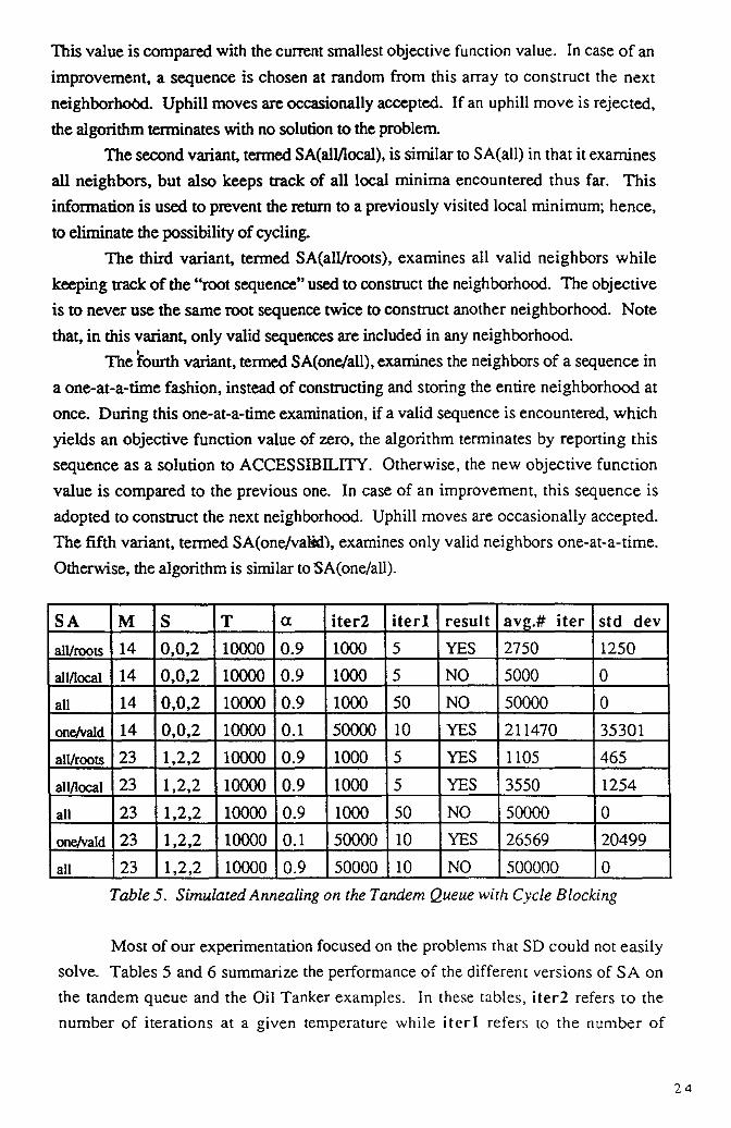
SA M S T a iter2 iterl result avg.# iter std dev

all/roots 14 0,0,2 10000 0.9 1000 5 YES 2750 1250

all/local 14 0,0,2 10000 0.9 1000 5 NO 5000 0

all 14 0,0,2 10000 0.9 1000 50 NO 50000 0

one/vald 14 0,0,2 10000 0.1 50000 10 YES 211470 35301

all/roots 23 1,2,2 10000 0.9 1000 5 YES 1105 465

all/local 23 1,2,2 10000 0.9 1000 5 YES 3550 1254

all 23 1,2,2 10000 0.9 1000 50 NO 50000 0

one/vald 23 1,2,2 10000 0.1 50000 10 YES 26569 20499

all 23 1,2,2 10000 0.9 50000 10 NO 500000

Table 5. Simulated Annealing on the Tandem Queue wi h Cycle Blocking

Most of our experimentation focused on the problems that SD could not easily

solve. Tables 5 and 6 summarize the performance of the different versions of SA on

the tandem queue and the Oil Tanker examples. In these tables, iter2 refers to the

number of iterations at a given temperature while iterl refers to the number of

24

temperature changes. T denotes the initial temperature. S depicts the target state. In

the following tables, a YES result indicates that a solution (event sequence) for

ACCESSIBILITY has been found. Similarly, a NO result indicates that no such

sequence has been identified.

S A M S T a iter2 iterl result avg.# iter std dev

all 24 12 10000 0.9 100 20 YES 12 1.15

all 50 25 10000 0.9 100 20 YES 25 18

all 80 40 10000 0.9 100 20 YES 40 32

all 100 50 10000 0.9 100 20 YES 50 24

one/vald 24 12 10000 0.9 1000 50 NO 50000 0

one/vald 50 25 10000 0.9 1000 50 NO 50000 0

one/vald 80 40 10000 0.9 10000 10 YES 81663 22438

one/vald 100 50 10000 0.9 10000 10 YES 50847 7954

Table 6. Simulated Annealing on the Oil Tanker Problem

M S CC T iterl iter2 Result avg# iter std dev

24 12 0.001 10000 50 1000 YES 2727 205

24 12 0.01 10000 50 1000 YES 2836 421

24 12 0.1 10000 50 kk000 YES 5196 833

24 12 0.5 10000 50 1900 YES 13754 1400

24 12 0.9 10000 50 1000 NO 50000 0

50 25 0.1 10000 50 1000 YES 6324 675

50 25 0.5 10000 50 1000 YES 15974 1744

50 25 0.9 10000 50 1000 NO 50000 0

50 25 0.1 100000 50 1000 YES 7186 832

5Q 25 0.1 10000 5 10000 YES 45067 2741

80 40 0.1 10000 10 10000 YES 55219 7939

100 50 0.1 10000 10 10000 YES 54492 4632

100 50 0.5 10000 50 1000 YES 18878 2386

100 50 0.9 10000 50 1000 NO 50000 0

150 75 0.1 10000 10 10000 NO 100000 0

150 75 0.1 10000 10 50000 NO 500000 0

150 75 0.5 10000 50 1000 NO 50000 0

Table 7. Impact of the Annealing Schedule

25

Table 7 shows the impact of the annealing schedule on the performance of the

algorithm in terms of the average total number of iterations. In this experiment,

SA(one/valid) is applied to the Oil Tanker Problem. Recall that M denotes the length of

the event sequence while S denotes the target state, which is the number of tankers

waiting to be berthed.

Two variants of the SA algorithm are compared using the tandem queue model.

In this experiment, T = 10000 and a = 0.9. The average number of iterations required

for different event sequences and target states are depicted in Table 8. The table shows

that, in general, SA(all) is faster than SA(one/valid); however, there are models where

only SA(one/valid) yields a solution. Note that an asterisk (*) indicates that the

algorithm failed to reach a solution within the total number of iterations.

M S iterl iter2 Avg # Iter

SA(one/valid)

std

dev

Avg # Iter

SA(all)

std

dev

10 3,0,1 20 100 1742 336 540 522

11 3,2,0 20 100 426 253 14 5

14 3,1,1 20 100 1300 629 96 59

14 0,0,2 10 50000 242265 96547 500000(*) 0

15 3,3,0 20 100 2473 3040 14 3

18 3,2,1 50 100 2212 1155 208 78

19 3,4,0 50 1000 4886 611 16 7

23 1,2,2 10 50000 43943 5439 500000 (*) 0

24 2,2,2 50 1000 17609 7895 50000 (*)

Table 8. Comparison of SA(one/valid) and SA(all)

Several conclusions can be drawn from our experimentation. First, the

importance of the initial solution (starting configuration) cannot be overemphasized.

Moreover, as the size of the event sequence grows larger, it becomes more and more

difficult to select a "good" starting configuration.

Second, the cooling schedule has a big impact on the performance of the

algorithm. We recommend to start at a relatively high temperature and conduct a large

number of iterations at each temperature before reducing it further.

Finally, for simple models and/or trivial states, a simple algorithm such as

SA(all) performs in a satisfactory fashion. For more complicated models, however, it

is recommended that a more sophisticated algorithm be used. Such an algorithm (e.g.,

SA(one/valid)) spends more effort at a given iteration in carefully selecting the

subsequent neighbors to investigate, thus avoiding unnecessary iterations.

26

6. CONCLUDING COMMENTS

In solving ACCESSIBILITY, SD and SA seem to be practical heuristic approaches. In

fact, SD was able to solve most of our test problems. However, there were situations

where SA solved ACCOPT, hence ACCESSIBILITY, whereas SD stopped without

finding an answer after a pre-specified number of iterations. We therefore conjecture

that SA will be a more useful technique when ACCESSIBILITY is addressed for more

complex models.

The biggest drawback of SA is that the approach must be customized to the

problem at hand. Even though we have proposed several variants for solving

ACCESSIBILITY (see Appendix B), the parameters of the algorithm (such as the

annealing schedule) should be modified to better exploit the structure of the model

under study.

Table 9 summarizes the algorithms that we have tested. A short comment is

also presented with each procedure. The table reflects our subjective ranking, going

from the worst algorithm to the best one.

ALGORITHM COMMENTS

Event Tree Arrays become too big even for a mainframe. Cannot

even consider sequences of length 15 for some models.

Dynamic

Programming

Similar problems with those of the Event Tree

Heuristic' state space explosion

SA(one/a11) Simple. Can be run on a PC. Unable to solve slightly

more complex problems.

SD Straightforward. Does not always reach a solution.

SA(all) Finds solution in cases where SD failed. Could be

slow for long sequences.

SA(all/local) Finds solution in more cases than SA(all). Also

slightly faster than SA(all).

SA(all/roots) Finds solutions to cases where SA(all) and SA(all/local)

fail. However, slower than both of them.

SA(one/valid) Simple. Runs on PC. Found solution for every

model. The best by far.

Table 9. Performance Summary

The theory of computational complexity provides a unifying framework for

assessing the difficulty of seemingly unrelated problems in structural analysis of

discrete event simulation models. Our work implies that it is highly unlikely that a

27

polynomial-time algorithm can be devised to verify such properties, with important

consequences for a wide range of modeling and analysis questions. This paper

examined special cases of the NP-hard problems discussed in Jacobson and Yucesan

[1994]. It was quickly discovered that most of the special cases, which are interesting

from a practical point of view, are still NP-hard. This, in turn, endorses the

development of heuristic approaches to address these problems. Several algorithms are

presented together with encouraging performances on a limited set of test problems.

Current research is focusing on refining these algorithms, and devising improved

heuristics for these and the other simulation-based NP-hard problems.

ACKNOWLEDGEMENTSThe second author gratefully acknowledges the support of INSEAD through the R&DProject # 2265R. The authors would also like to thank Katrina Maxwell-Balloux forher invaluable programming assistance in conducting the experiments.

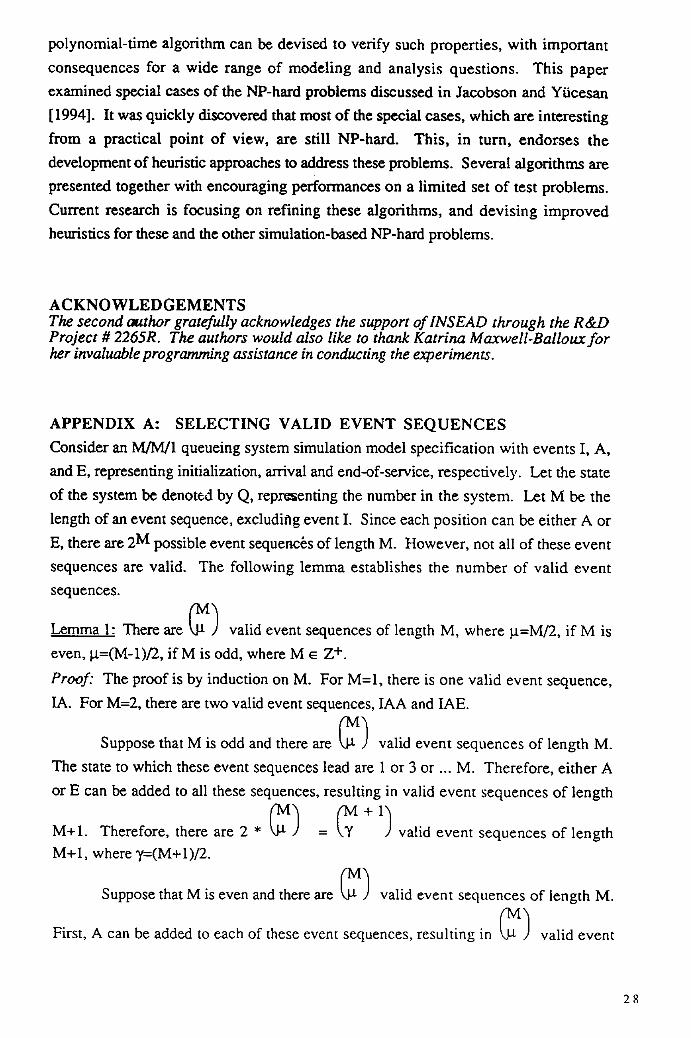
APPENDIX A: SELECTING VALID EVENT SEQUENCES

Consider an M/M/1 queueing system simulation model specification with events I, A,

and E, representing initialization, arrival and end-of-service, respectively. Let the state

of the system be denoted by Q, representing the number in the system. Let M be the

length of an event sequence, excluding event I. Since each position can be either A or

E, there are 2M possible event sequences of length M. However, not all of these event

sequences are valid. The following lemma establishes the number of valid event

sequences.

Lemma 1: There are/ valid event sequences of length M, where 1.i.M/2, if M is

even, i.t=(M-1)/2, if M is odd, where M E Z.

Proof: The proof is by induction on M. For M=1, there is one valid event sequence,

IA. For M=2, there are two valid event sequences, IAA and IAE.

Suppose that M is odd and there are 11 ) valid event sequences of length M.

The state to which these event sequences lead are 1 or 3 or ... M. Therefore, either A

or E can be added to all these sequences, resultingNy4 + 1 in valid event sequences of length11V141 ) = ()

M+1. Therefore, there are 2 * ) valid event sequences of lengthM+1, where y.(M+ 1)/2.

Suppose that M is even and there are Git) valid event sequences of length M.

First, A can be added to each of these event sequences, resulting in !- 1 ) valid event

28

sequences of length M+1. Second, note that the state to which these event sequences

lead are 0 or 2 or ... M. All these sequences, except the ones terminating in Q=0, can

have event E' appended to them, resulting in valid sequences of length M+1. Note that— 1)

there are .11 — I ) valid event sequences of length M resulting in final state Q=2,1M — 2)

Jl — 2 ) valid event sequences of length M resulting in final state Q=4, and so on,

until there is one valid event sequence of length M resulting in final state Q=M, namely

all events A. This follows by noting that to obtain these final states, there must be more

arrival events (A) than end-of-service events (E); hence, these arrival events must be

adjacent in the sequence. They can therefore be clustered together and can be viewed as(M 4- 1)

a single unit in the event sequences. Summing these values results in x ), where

ic.(M+1)/2. q

The following lemma shows that the number valid event sequences for a single-

server queue grows exponentially in M, for M large.

Lemma2: The number of valid event sequences of length M is 0(2 M / M la) as M

approaches infinity.

Proof: Suppose that M is even. Then l , where j.t=M/2, can be written as

MiA(M/2)02. By Stirling's formula, for large M,

MK(M/2)02 [MM+0.5 e'M (270 1/2M(W2)M+1 e-M (270]2M (2/7cm)1n

= 0(2M / M 1t2) for large M. q

From Lemma 2, since there are 2 M event sequences in total, then, as M

approaches infinity, the ratio of valid event sequences to the total number of event

sequences is 0(1/M 1/2). Therefore, the number of valid event sequences is a slowly

decreasing fraction of the total number of event sequences, where this fraction is 1/M1a

for M large.

APPENDIX B: VARIANTS OF THE SA ALGORITHM

The five variants of the SA algorithm are presented in pseudo-code format. In each

description, the initial part of the algorithm, where the data about the model

specification and the parameters are read, is omitted.

29

SA(one/valid)Set initial temperature, T;Set the temperature change coefficient, 0 < a < I;Set the desired number of temperature changes, iterl;Set the desired number of iterations at a given temperature, iter2;

Set temperature change counter, t 0;

RepeatSet counter, n 0;Repeat

Generate a sequence, y, a neighbor of x;If (y is a valid sequence) then do:

BeginIf f(y) = 0 then STOP (report event sequence);Calculate 8 = f(y)-f(x);

If 8 < 0 then x y;Elseif rnd {0,1} < exp{-8/T) then x y;Endif

End;n n + 1

Until n = iter2;t 4-- t + 1;T aT;

Until t = iterl;Exit (no solution found).

SA(one/a11)Set initial temperature, T;Set the temperature change coefficient, 0 < a < 1;Set the desired number of temperature changes, iterl;Set the desired number of iterations at a given temperature, iter2;


RepeatSet counter, n 4-- 0;

RepeatGenerate a sequence, y, a neighbor of x;If f(y) = 0 then STOP (report event sequenc0:Calculate 8 = f(y)-f(x);If 8 < 0 then x y;Elseif rnd (0,1 } < exp{-8M then x y;Endifn E- n+ 1

Until n = iter2;t4—t+1;T aT;

Until t = iterl;End (no solution found).

SA(211)Set initial temperature, T;Set the temperature change coefficient, 0 < a < 1;Set the desired number of temperature changes, iterl ;Set the desired number of iterations at a given temperature, iter2;

30



Generate sequences, yi, all neighbors of x;For each sequence in the neighborhood, do:Begin

If f(y) = 0 then STOP (report event sequence);End;Pick the sequence(s), yj, with the smallest f(y);Calculate 8 = f(y)-f(x);If 8 < 0 then doBegin

Store all yj in an array;Pick one sequence at random to construct next

neighborhood;End;Else if md(0,1) < exp{-8/1"} then doBegin


neighborhood;End;Else STOP(no solution found). /*stuck at a local minimum*/Endifn +- n + 1

Until n = iter2;t t + 1;T aT;


SA(all/local)Set initial temperature, T;Set the temperature change coefficient, 0 < a < 1;Set the desired number of temperature changes, iterl;Set the desired number of iterations at a given temperature, iter2;



Generate sequences, yi, all neighbors of x;For each sequence in the neighborhood, do:Begin

If f(y) = 0 then STOP (report event sequence);End;Pick the sequence(s), yj, with the smallest f(y);For all local minima encountered thus far, z, doBegin

Calculate 5 = f(y)-f(z);End;If any 8 < 0 then do

31

BeginStore all yj in an array;Pick one sequence at random to construct next

neighborhood;End;Else if md(0,1) < exp{-8/T} then doBegin


neighborhood;Add the old sequence to the list of local minima;

End;Else STOP(no solution found). /*stuck at a local minimum*/Endifn n + 1

Until n = iter2;t t + 1;T E- aT;

Until t ='iterl;Exit (no solution found).

S A (all/roots)Set initial temperature, T;Set the temperature change coefficient, 0 < a < 1;Set the desired number of temperature changes, iterl;Set the desired number of iterations at a given temperature, iter2;



Generate sequences, yi, all neighbors of x;For each valid sequence in the neighborhood, do:Begin

If f(y) = 0 then STOP (report event sequence);End;Pick the sequence(s), yj, with the smallest f(y);For all local minima encountered thus far, z, doBegin

Calculate 5 = f(y)-f(z);End;If any 8 < 0 then doBegin


neighborhood;End;Else if md{0,1} < exp{-61T} then doBegin


neighborhood;Add the old sequence to the list of local minima;

End;Else STOP(no solution found). /*stuck at a local minimum*/

3

Endifn n + 1

Until n = iter2;tEt + 1;T +– aT;


REFERENCES

Balci, 0. and R.E. Nance (1987) "Simulation Model Development Environments: AResearch Prototype". Journal of the Operational Research Society. 38.8, 753-763.

Balmer, D.W. and R.J. Paul (1990) "Integrated Support Environments for SimulationModeling." Proceedings of the 1990 Winter Simulation Conference. Balci, Sadowski,and Nance, Eds. 243-249.

Bratley, P., B.L. Fox, and L.E. Schrage (1987) A Guide to Simulation. Springer-Verlag. New York, NY.

Eglese, R.W. (1990) "Simulated Annealing: A Tool for Operational Research."European Journal of Operational Research. 46, 271-281.

Evans, J.W., J.F. Wallace, and J.L. Sutherland (1967) Simulation Using DigitalComputers. Prentice Hall. Englewood Cliffs, NJ.

Fox, B.L. and D.M. Landi (1968) "An Algorithm for Identifying the ErgodicSubchains and Transient States of a 5,tochastic Matrix." Communications of the ACM.11.9, 619-621.

Garey, M.R. and D.S. Johnson (1979) Computers and Intractability: A Guide to theTheory of NP-Completeness. W.H. Freemann and Company. New York, NY.

Glasserman, P. and D.D. Yao (1992) "Monotonicity in Generalized Semi-MarkovProcesses". Math of Operations Research. Vol.17.1. pp.1-21.

Glynn, P.W. and D.L. Iglehart (1988) "Simulation Methods for Queues: AnOverview." Queueing Systems: Theory and Applications. 3, 221-256.

Ho, Y.-C. and X.-R. Cao (1991) Perturbation Analysis of Discrete Event DynamicSystems. Kluwer Academic Publishers. Dordrecht, The Netherlands.

Jacobson, S.H. and E. Yucesan (1994) "On the Complexity of Verifying StructuralProperties of Discrete Event Simulation Models." Submitted for publication.

Karlin, S. and H.M. Taylor (1975) A First Course in Stochastic Processes. SecondEdition. Academic Press.New York, NY.

Law, A.M. and W.D. Kelton. (1991) Simulation Modeling and Analysis. SecondEdition. McGraw-Hill. New York, NY.

Nance, R.E. (1981) "The Time and State Relationships in Simulation Modeling."Communications of the ACM. 24.4, 173-179.

33

Onvural, R.O. and H.G. Perros (1986) "On Equivalencies of Blocking Mechanismsin Queueing Networks with Blocking." Operations Research Letters. 5.6, 293-297.

Overstreet, C.M. (1982) "Model Specification and Analysis for Discrete EventSimulations." Unpublished PhD Dissertation. Department of Computer Science.Virginia Tech. Blacksburg, VA.

Overstreet, C.M. and R.E. Nance (1985) "A Specification Language to Assist inAnalysis of Discrete Event Simulation Models." Communications of the ACM. 28.2,190-201.

Pegden, C.D., R.E. Shannon, and R.P. Sadowski (1990) Introduction to SIMAN.Systems Modeling Corporation. Pittsburgh, PA.

Pritsker, A.A.B. (1986) Introduction to Simulation and SLAM II. 3rd Edition. JohnWiley & Sons. New York, NY.

Schruben, L. (1992) Sigma: A Graphical Simulation System. 2nd Edition. TheScientific Press. San Francisco, CA.

Som, T.K. and R.G. Sargent (1989) "A Formal Development of Event Graphs as anAid to Structured and Efficient Simulation Programs." ORSA Journal on Computing.1.2, 107-125.

Suri, R. (1989) "Perturbation Analysis: The State of the Art and Research IssuesExplained via the GI/G/1 Queue." Proceedings of the IEEE. 77.1, 114-136.

Whitner, R.B. and 0. Balci (1989) "Guidelines for Selecting and Using SimulationModel Verification Techniques." Proceedings of the Winter Simulation Conference.MacNair, Musselman, and Heidelbetger, Eds. 559-568.

Yucesan, E. (1989) "Simulation Graphs for the Design and Analysis of Discrete EventSimulation Models." Unpublished Phb Dissertation. School of Operations Researchand Industrial Engineering, Cornell University. Ithaca, NY.

Yucesan, E. and S.H. Jacobson (1992) "Building Correct Simulation Models isDifficult." Proceedings of the Winter Simulation Conference. Swain, Goldsman,Crain, and Wilson, Eds. 783-790.

Yucesan, E. and L. Schruben (1993) "Modeling Paradigms in Discrete EventSimulation." Operations Research Letters. 13(June), 265-275.

Zeigler, B.P. (1976) Theory of Modelling and Simulation. John Wiley. New York,NY.

34

Documents

INTRACTABLE STRUCTURAL ISSUES IN DISCRETE EVENT SIMULATION