Intertemporal Substitutionin Labor Force Participation:

Evidence from Policy Discontinuities

Dayanand ManoliUCLA & NBER

Andrea WeberUniversity of Mannheim

August 25, 2010

Abstract

This paper presents new empirical evidence on intertemporal labor supply elastic-ities. We use administrative data on the census of private sector employees in Austriaand variation from mandated discontinuous changes in retirement bene�ts from theAustrian pension system. We �rst present graphical evidence documenting delays inretirement in response to the policy discontinuities. Next, based on the empiricalevidence, we develop a model of career length decisions. Using a semiparametric esti-mator that exploits the graphical evidence, we estimate a relatively low intertemporallabor supply elasticity of 0:30.

1

1 Introduction

The theory of intertemporal labor supply is the workhorse theory of dynamic labor sup-

ply decisions in economics. In various applications of this theory in macroeconomics, labor

economics and public economics, the intertemporal labor supply elasticity plays a central

role in understanding business cycle �uctuations, life-cycle labor supply, and responses

to income tax and transfer programs. Despite its importance in many macroeconomic

and microeconomic models, there is wide-spread debate regarding the magnitude of this

intertemporal labor supply elasticity with the higher and lower elasticities having vastly

di¤erent policy implications.

In this study, we provide new empirical evidence on intertemporal labor supply elas-

ticities using responses to policy discontinuities in retirement bene�ts in Austria. We �rst

present nonparametric graphical evidence documenting individuals�labor supply responses

to the policy discontinuities. Next, we develop a semiparametric elasticity estimator that

exploits the observed labor supply responses. Based on the observed patterns in individ-

uals� retirement decisions, we estimate an intertemporal labor supply elasticity of 0:30.

Thus, standard intertemporal labor supply models that rely on high intertemporal labor

supply elasticities would be at odds with the observed data presented in this study.

There has been signi�cant research on intertemporal labor supply elasticities yielding

a wide range of values.1. Some recent e¤orts to distinguish between higher and lower

elasticities have focused on the distinction between the intensive and extensive margins

of labor supply decisions (see Rogerson and Wallenius (2009) and Ljungqvist and Sargent

(2010)2). Intuitively, elasticities based on intensive margin (hours of work in a given time

period) decisions may be small while elasticities based on extensive margin (career length)

decisions may be large. While some previous studies have focused only on intensive margin

labor supply decisions, we are able to estimate an intertemporal labor supply elasticity while

focusing explicitly on extensive margin decisions. In particular, we estimate an extensive

margin Frisch elasticity, or more intuitively, an elasticity of career length with respect to

1See Blundell and MaCurdy (1999) for a survey of the microeconomic evidence of intertemporal sub-stitution in labor supply. For macroeconomic evidence, see Prescott (2006), Mulligan (1999), Ohanian etal (2008), Rogerson and Wallenius (2009) and Ljungqvist et al (2006). Keane and Rogerson (2010) surveyboth microeconomic and macroeconomic evidence on intertemporal labor supply elasticities; these authorsalso discuss e¤orts to reconcile higher elasticities based on macroeconomic evidence with lower elasticitiesfrom microeconomic evidence.

2In earlier research, Heckman (1993) emphasizes the distinction between intensive and extensive marginlabor supply decisions.

2

anticipated wages.

The policy discontinuities exploited in this study arise because retirement bene�ts in

Austria increase discontinuously once individuals complete speci�c threshold amounts of

tenure prior to their retirements. We examine behavior before and after these tenure

thresholds to determine if individuals extend their careers in response to the anticipated

discontinuous increases in bene�ts. Graphical evidence indicates excess retirements just

after the thresholds and reduced retirements just prior to the thresholds. We then use a

standard labor supply model to develop semiparametric estimator for the elasticity of career

length with respect to anticipated wages based on the graphical evidence.3 While previ-

ous structural estimation strategies have often been forced to make speci�c distributional

assumptions to recover structural parameters, we are able to recover a policy-relevant struc-

tural parameter from a quasi-experimental design without having to make these parametric

assumptions.

This paper is organized as follows. Section 2 discusses both the institutional background

regarding the Austrian pension system and the administrative data from the Austrian

Social Security Database. Section 3 presents a nonparametric graphical analysis of the

data. Section 4 develops an intertemporal labor supply model based on the empirical

evidence presented in section 3. Section 5 develops the elasticity estimation strategy and

then presents the estimation results. Section 6 concludes.

2 Institutional Background & Data

2.1 Retirement Bene�ts in Austria

There are two forms of government-mandated retirement bene�ts in Austria: (1) government-

provided pension bene�ts and (2) employer-provided severance payments. We start with

the description of severance payments since these payments are the primary focus of the

current study. The employer-provided severance payments are made to private sector em-

ployees who have accumulated su¢ cient years of tenure by the time of their retirement.

Tenure is de�ned as uninterrupted employment time with a given employer and retirement

is based on claiming a government-provided pension. The payments must be made within

4 weeks of claiming a pension according to the following schedule. If an employee has

3While this estimator relies on discontinuities in individuals�budget constraints, it is similar in spirit toprevious bunching estimators that exploit kinks in individuals�budget constraints (see Saez (1999, 2009)and Chetty et al (2009)).

3

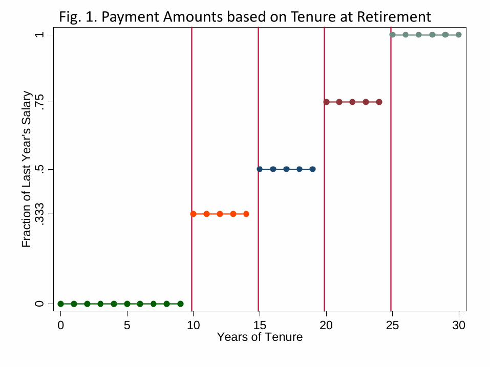
accumulated at least 10 years of tenure with her employer by the time of retirement, the

employer must pay one third of the worker�s last year�s salary. This fraction increases from

one third to one half, three quarters and one at 15, 20 and 25 years of tenure respectively.

This schedule for the severance payments is illustrated in Figure 1. The payments are

made in lump-sum and, since payments are based on an employee�s salary, overtime com-

pensation and other non-salary payments are not included when determining the amounts

of the payments. Provisions to make these payments come from funds that employers are

mandated to hold based on the total number of employees. Severance payments are also

made to individuals who are involuntarily separated (i.e. laid o¤) from their �rms if the

individuals have accumulated su¢ cient years of tenure prior to the separation. The only

voluntary separation that leads to a severance payment, however, is retirement.4

The Austrian income tax system, which is based on individual taxation, applies par-

ticular rules to tax income from severance payments. Speci�cally, all mandated severance

payments are exempt from social security contributions and subject to a tax rate of 6%.

The income taxation of the severance payments di¤ers from the general income tax rules.

Generally, gross monthly earnings net of social security contributions 5 are subject to the

income tax with marginal tax rates in the di¤erent tax brackets of 0%, 21%, 31% 41% and

50%.6 7

Because the timing of the severance payments relates to pension claiming, eligibility

for government-provided retirement pensions interacts with the severance payment system.

Austria has a public pension system that automatically enrolls every person employed in

the private sector. Fixed pension contributions are withheld from each individual�s wage

and annuitized bene�ts during retirement are then based on prior contributions (earnings

histories). Replacement rates from the annual payments are roughly 75% of pre-retirement

earnings and there are no actuarial adjustments for delaying retirement to a later age.

Individuals can retire by claiming Disability pensions, Early Retirement pensions and Old

Age pensions. Eligibility for each of these pensions depends on an individual�s age and

4For more details regarding the severance payments at times of unemployment, see Card, Chetty andWeber (2007).

5Contributions for pension, health, unemployment, and accident insurance of 39% are split in halfbetween employer and employee and the employee�s share is withheld from gross annual earnings up to acontribution cap.

6These tax brackets are based on legislation in 2002; there have subsequently been relatively smallchanges due to several small tax reforms.

7Additionally, Austrian employees are typically paid 13th and 14th monthly wage payments in Juneand December. These payments, up to an amount of one sixth of annual wage income, are also subject toa 6% tax rate; amounts in excess of one sixth of annual income are subject to the regular income tax rates.

4

gender, as well as having a su¢ cient number of contribution years. Beginning at age 55,

private sector male and female employees can retire by claiming Disability pensions, where

disability is based on reduced working capacity of 50% relative to someone of a similar

educational background. At age 55, women also become eligible to claim Early Retirement

pensions, but the Early Retirement Age is age 60 for men. Lastly, men and women become

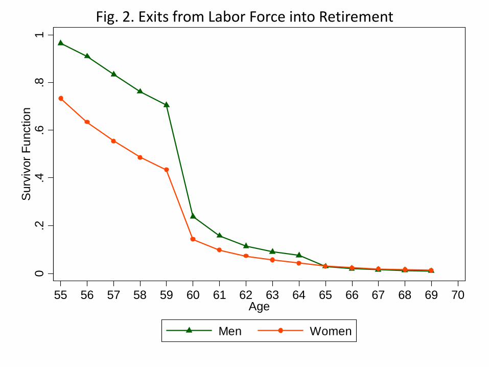
eligible for Old Age pensions at age 65 and 60 respectively.8 Figure 2 illustrates survival

functions for entry into the pension system for the sample of private sector employees. The

graphs are presented separately for men and women given the di¤erent eligibility ages.

The survival functions illustrate sharp declines at ages 60 and 65 highlighting a signi�cant

amount of entry into the pension system once individuals become eligible for the Early

Retirement and Old Age pensions. Additionally, the �gure demonstrates that, for both

men and women, most retirements occur between ages 55 and 60. Further, the graph

shows that roughly 25% of the male sample retire by claiming disability pensions prior to

age 60.

2.2 Administrative Data & Sample Restrictions

Our empirical analysis is based on administrative registers from the Austrian Social

Security Database (see Zweimüller et al (2009)), which is collected with the principle aim

of verifying individual pension claims. This implies that the data provide longitudinal

information for the universe of private sector workers in Austria throughout their working

lives. Speci�cally, information on employment and earnings as well as other labor market

states relevant for computing insurance years such as military service, unemployment, and

maternity leave is collected. Detailed electronic records with employer identi�ers that

allow the measurement of tenure are recorded the period from 1972 onwards; here we

use information up to 2006. For the years prior to 1972 retrospective information on

insurance relevant states is available for all individuals who have retired by the end of the

observation period. Together the two data sets provide information on complete earnings

and employment careers of retirees. Because �rm identi�ers are available only from 1972

onwards, uncensored tenure can only be measured for jobs starting after January 1, 1972.

To investigate the e¤ect of severance pay eligibility on retirement decisions we consider

all individuals born between 1930 and 1945. For these individuals we observe su¢ ciently

8Bene�ts from disability and early retirement are entirely withdrawn if an individual earns more thanabout 300 Euros per month, therefore we see very few individuals returning to the labor force once theyare retired.

5

long uncensored tenure at retirement.9 We focus on workers who are still employed after

their 55th birthday and follow them until entry into retirement or up to the age of 70.

We make several restrictions to the original sample of about 650,000 workers, which are

summarized in the top panel of Table 1. Most importantly, we exclude individuals who

worked as civil servants or whose last job was in construction, because they are subject

to di¤erent pension and severance pay rules. As we are interested in tenure at retirement,

we further exclude workers with left censored tenure at retirement and we only consider

retirement entries which occur within 6 months of the worker�s last job. Individuals with

longer gaps between employment and retirement are only followed until the end of the last

employment. With these restrictions, we have a �nal sample of 269; 411 retiring individuals.

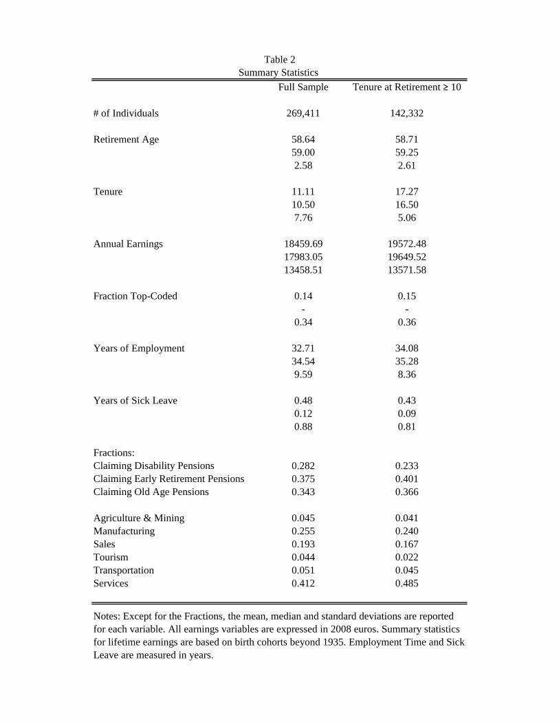
Table 2 presents summary statistics separately for the full retirement sample and for

the sub-sample of individuals with more than 10 years of tenure at retirement, who are

eligible for severance pay. The median retirement age is at 59 years in both groups, which

re�ects that most individuals retire through disability or early retirement (28% and 38%

in the full sample, respectively).10 Years of employment and annual earnings in the last

year before retirement are slightly higher for workers with longer tenure and these workers

also appear to be of better health given their average time spent in sick leave. Overall

the di¤erences between both groups are minor. Earnings relevant for the calculation of

retirement bene�ts and therefore reported by the ASSD are top coded; roughly 14% of the

sample has censored earnings at retirement.

3 Nonparametric Graphical Analysis

In this section we present graphical evidence on the individual labor supply responses

to the severance payment thresholds at retirement. We start with a discussion of patterns

in the distribution of tenure at retirement that is observed in the raw data. To con�rm

that these patterns correspond to reactions to the severance payment rule, we present three

pieces of empirical evidence. First, we investigate the variation of other observables around

the tenure thresholds and examine whether or not this variation in other observables can

explain the observed patterns in the distribution of tenure at retirement. Second, we exam-

9In addition, these individuals retire after the pension reform in 1985, which changed the assessmentbasis for bene�t calculation and the thereby the type of information recorded.10The actual share of retirements through early retirement is higher than the presented number, as

separate insurance categories for early retirement are only recorded as of 07/1993 and individuals retiringbefore the statutory pension age before that are coded as old age pension entries.

6

ine whether decisions earlier in life such as job changes at particular ages are responsible for

the retirement patterns. Finally, we investigate how the patterns in tenure at retirement

vary across various subgroups within the sample. We con�rm that there is heterogeneity

in the retirement patterns such that there are less (more) distinctive patterns amongst

groups that we expect to be less (more) responsive to the severance payments. While this

section focuses on highlighting the empirical evidence on labor supply responses to the

severance payments, the next section presents a model of retirement decisions motivated

by the empirical evidence.

3.1 Distribution of Tenure at Retirement

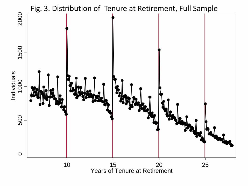
Figure 3 presents the distribution of tenure at retirement for the full sample with the

number of individuals on the vertical axis and years of tenure at retirement on the hor-

izontal axis; tenure at retirement is measured at a monthly frequency. Several features

are immediately evident from this graph. First, the plot shows discontinuous spikes in the

number of retirements at the tenure thresholds. Second, there are dips in the number of

retirements just before the tenure thresholds, which are generally concentrated within 1

year before the threshold. These patterns are regularly repeated at each tenure threshold

but are not apparent at any other point in the tenure distribution. This evidence suggests

that individuals who would have retired just before the thresholds in the absence of the

severance pay discontinuities end up delaying their retirements until they just qualify for

the (larger) severance payments. The plot also indicates a seasonal pattern illustrated by

small spikes in the number of retirement at each integer value of years of tenure at retire-

ment. The seasonality can be explained by a relatively large fraction job starts in January

and corresponding retirement exits in December.

Some noteworthy features are indicated by the pattern in Figure 3. First, the dips and

spikes around the tenure thresholds are clearly separated from each other. This indicates

that labor supply responses to each tenure threshold occur in a relatively narrow time

window around the threshold. An impact of the severance pay schedule on intertemporal

labor supply decisions beyond a �ve-year horizon is therefore not supported by the data.

Second, the plot does not illustrate any evidence of income e¤ects. In the presence of

detectable income e¤ects, individuals receiving larger severance payments would be more

likely to retire than those receiving smaller payments. This would lead to discrete level

changes between the tenure thresholds in the distribution of tenure at retirement since

7

some individuals have su¢ cient tenure to receive a payment when they become eligible for

retirement. Additionally, if wealth e¤ects from the severance payments are relatively large,

then individuals who qualify for the severance payments would end up retiring earlier than

they would have in the absence of the severance payments. The observed patterns therefore

suggest that wealth e¤ects from the severance payments are relatively small. Third, even

though there are decreases prior to the thresholds, the frequency of retirements never goes

to zero just prior to the thresholds. This means there appears to be a substantial number of

individuals who are unresponsive to the severance pay system at retirement. Our analysis

of heterogeneity in labor supply responses will therefore concentrate on identifying the

unresponsive groups; we will examine how health, earnings, �rm size and job rigidity relate

to responsiveness to the severance pay thresholds.

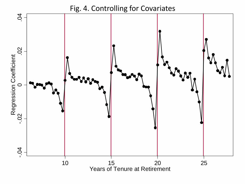
3.2 Accounting for Covariates

We exploit panel variation in the probability of retirement to examine whether or not

other observable characteristics change around the tenure thresholds. In particular, we

estimate the following regression

rit =34P�=0

�d� +Xit� + �it

where rit is an indicator equal to 1 if individual i retires within time period t and d� is an

indicator equal to 1 if the individual�s tenure at time t equals � . For computational reasons,

time is measured at a quarterly frequency at January 1st, April 1st, July 1st and October

1st instead of the monthly frequency presented in Figure 3. We include a large set of time-

varying control variables Xit relating to age, calendar years, industry, region, seasonality,

earnings histories, �rm characteristics, health and experience.11 The set of observations per

individual covers all quarters from age 55 to retirement or age 70. Thus the sample used for

estimation includes all 380,737 individuals left at the last step of sample selection in Table

1, not only those observed retiring within 6 month of their last job. Including all job exits

11Firm size is grouped into the following categories: � 5, 6�10; 11�25; 26�99; 100�499; 500�999;� 1000.Health status through age 54 is based on the following categories of sick leave through age 54: � 0:5 years,0:5� 1 years, 1� 2 years, and � 2 years. Health in the current quarter is based on the following categoriesfor sick leave in the current quarter: 0 days, 1 � 30 days, 31 � 60 days, and � 61 days. Earnings growthdummies are based on positive, negative, or zero growth relative to earnings in the corresponding quarter.Quarterly earnings for individuals with continuous employment during a calendar year are equal to totalannual earnings divided by 4. Earnings for individuals retiring at the beginning of a quarter are set equalto earnings from the previous quarter. For women, the base controls also include a dummy for having kids.

8

allows us to examine whether or not regularities in general job exits (as opposed to just

retirements) after 5, 10, 15, ... year intervals are responsible for the observed retirement

patterns in Figure 3.

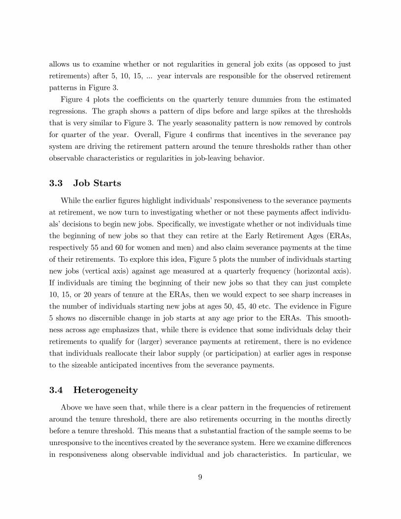
Figure 4 plots the coe¢ cients on the quarterly tenure dummies from the estimated

regressions. The graph shows a pattern of dips before and large spikes at the thresholds

that is very similar to Figure 3. The yearly seasonality pattern is now removed by controls

for quarter of the year. Overall, Figure 4 con�rms that incentives in the severance pay

system are driving the retirement pattern around the tenure thresholds rather than other

observable characteristics or regularities in job-leaving behavior.

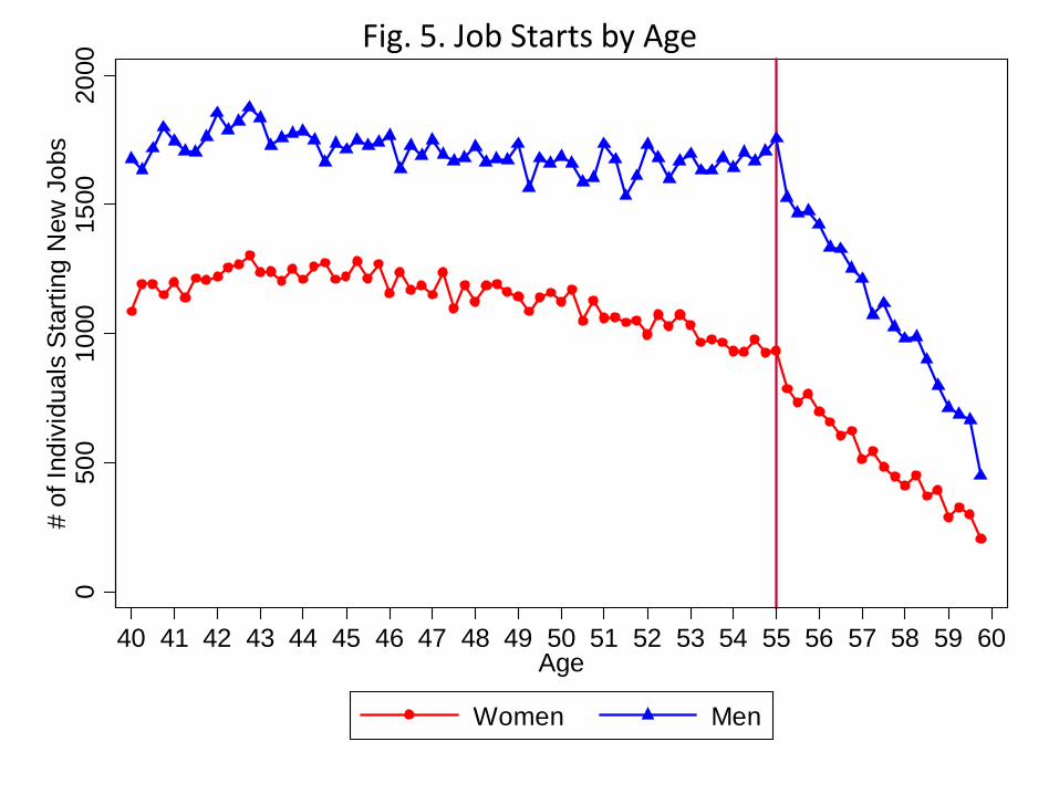
3.3 Job Starts

While the earlier �gures highlight individuals�responsiveness to the severance payments

at retirement, we now turn to investigating whether or not these payments a¤ect individu-

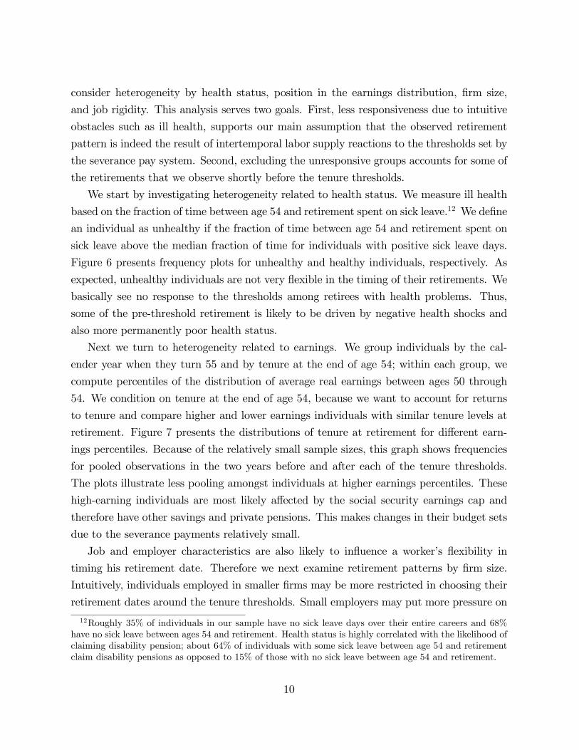
als�decisions to begin new jobs. Speci�cally, we investigate whether or not individuals time

the beginning of new jobs so that they can retire at the Early Retirement Ages (ERAs,

respectively 55 and 60 for women and men) and also claim severance payments at the time

of their retirements. To explore this idea, Figure 5 plots the number of individuals starting

new jobs (vertical axis) against age measured at a quarterly frequency (horizontal axis).

If individuals are timing the beginning of their new jobs so that they can just complete

10, 15, or 20 years of tenure at the ERAs, then we would expect to see sharp increases in

the number of individuals starting new jobs at ages 50, 45, 40 etc. The evidence in Figure

5 shows no discernible change in job starts at any age prior to the ERAs. This smooth-

ness across age emphasizes that, while there is evidence that some individuals delay their

retirements to qualify for (larger) severance payments at retirement, there is no evidence

that individuals reallocate their labor supply (or participation) at earlier ages in response

to the sizeable anticipated incentives from the severance payments.

3.4 Heterogeneity

Above we have seen that, while there is a clear pattern in the frequencies of retirement

around the tenure threshold, there are also retirements occurring in the months directly

before a tenure threshold. This means that a substantial fraction of the sample seems to be

unresponsive to the incentives created by the severance system. Here we examine di¤erences

in responsiveness along observable individual and job characteristics. In particular, we

9

consider heterogeneity by health status, position in the earnings distribution, �rm size,

and job rigidity. This analysis serves two goals. First, less responsiveness due to intuitive

obstacles such as ill health, supports our main assumption that the observed retirement

pattern is indeed the result of intertemporal labor supply reactions to the thresholds set by

the severance pay system. Second, excluding the unresponsive groups accounts for some of

the retirements that we observe shortly before the tenure thresholds.

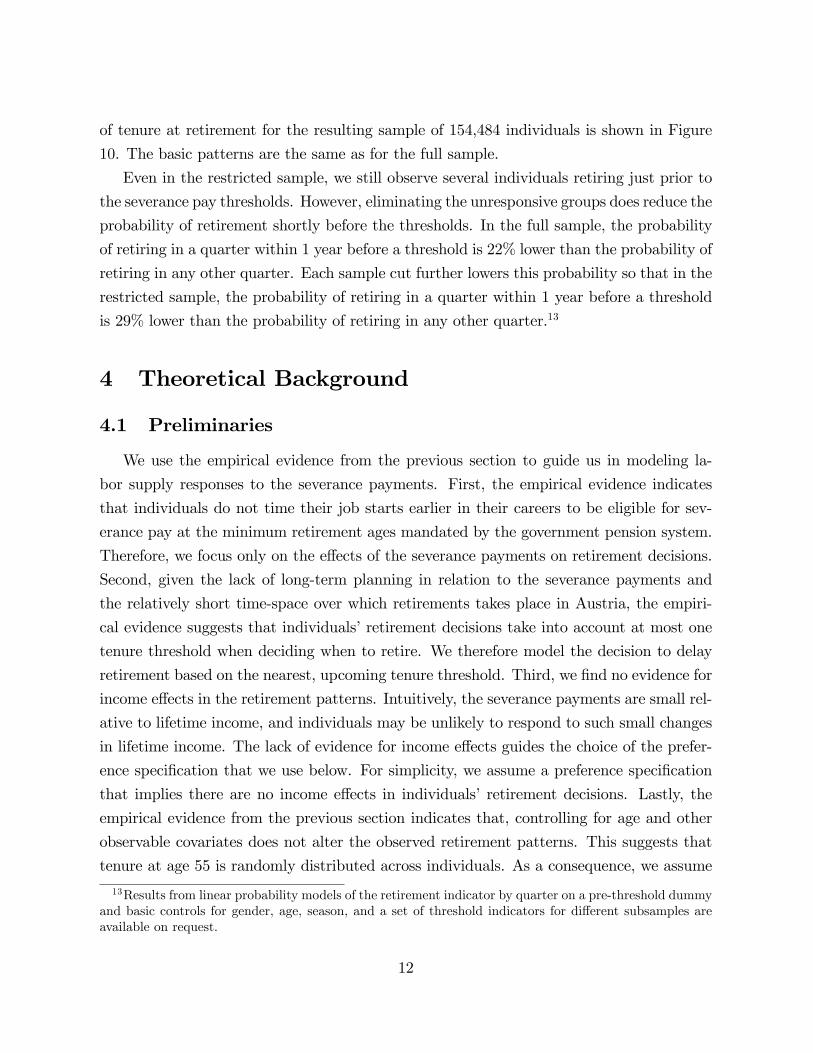
We start by investigating heterogeneity related to health status. We measure ill health

based on the fraction of time between age 54 and retirement spent on sick leave.12 We de�ne

an individual as unhealthy if the fraction of time between age 54 and retirement spent on

sick leave above the median fraction of time for individuals with positive sick leave days.

Figure 6 presents frequency plots for unhealthy and healthy individuals, respectively. As

expected, unhealthy individuals are not very �exible in the timing of their retirements. We

basically see no response to the thresholds among retirees with health problems. Thus,

some of the pre-threshold retirement is likely to be driven by negative health shocks and

also more permanently poor health status.

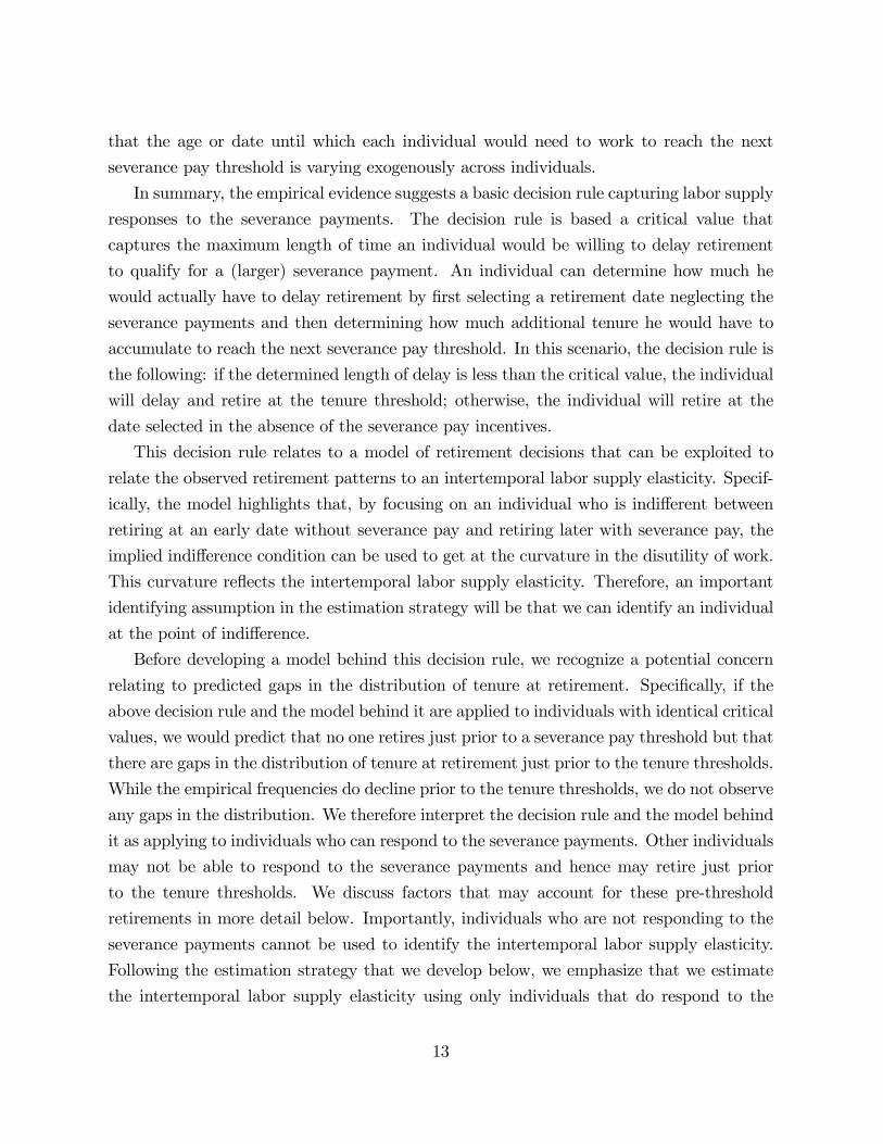
Next we turn to heterogeneity related to earnings. We group individuals by the cal-

ender year when they turn 55 and by tenure at the end of age 54; within each group, we

compute percentiles of the distribution of average real earnings between ages 50 through

54. We condition on tenure at the end of age 54, because we want to account for returns

to tenure and compare higher and lower earnings individuals with similar tenure levels at

retirement. Figure 7 presents the distributions of tenure at retirement for di¤erent earn-

ings percentiles. Because of the relatively small sample sizes, this graph shows frequencies

for pooled observations in the two years before and after each of the tenure thresholds.

The plots illustrate less pooling amongst individuals at higher earnings percentiles. These

high-earning individuals are most likely a¤ected by the social security earnings cap and

therefore have other savings and private pensions. This makes changes in their budget sets

due to the severance payments relatively small.

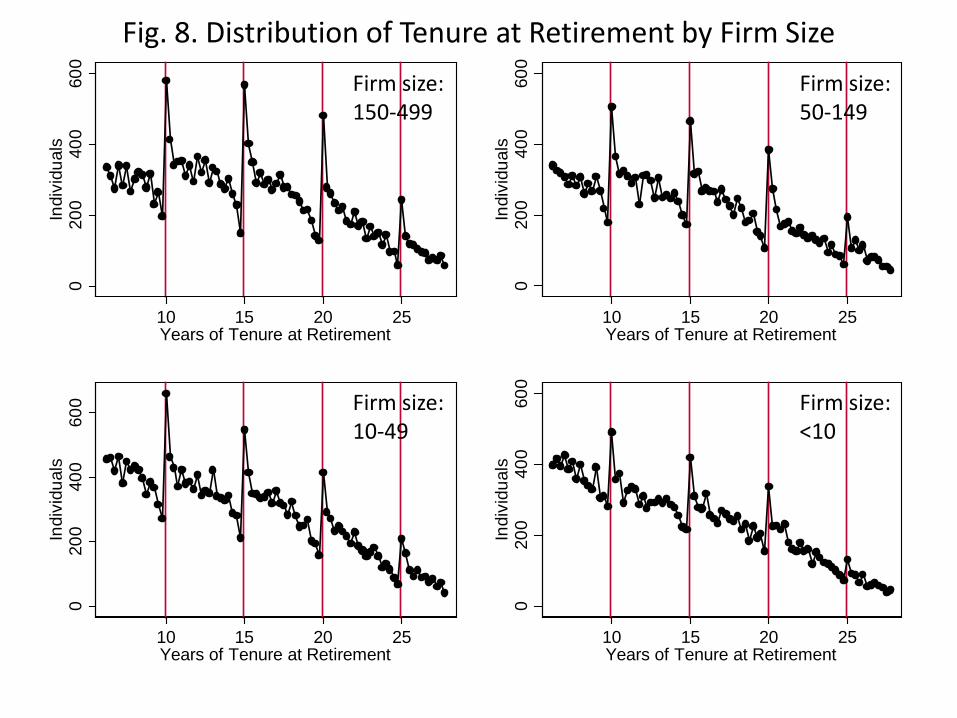
Job and employer characteristics are also likely to in�uence a worker�s �exibility in

timing his retirement date. Therefore we next examine retirement patterns by �rm size.

Intuitively, individuals employed in smaller �rms may be more restricted in choosing their

retirement dates around the tenure thresholds. Small employers may put more pressure on

12Roughly 35% of individuals in our sample have no sick leave days over their entire careers and 68%have no sick leave between ages 54 and retirement. Health status is highly correlated with the likelihood ofclaiming disability pension; about 64% of individuals with some sick leave between age 54 and retirementclaim disability pensions as opposed to 15% of those with no sick leave between age 54 and retirement.

10

their employees to retire prior to qualifying for a (larger) severance payment. Additionally,

employees at smaller �rms may have less ability to leave their �rms just after reaching a

tenure threshold since their employers may rely on them to complete their projects since

there are fewer substitutable employees available to do so. The evidence presented in Figure

8 is consistent with these intuitions as the plots indicate that the pre-threshold dips and

post-threshold spikes increase monotonically with �rm size.

As �rm size plays a considerable role for individual retirement decisions, we examine

also other rigidities that may be imposed by an individual�s job situation. In particular, we

use �rm level information on job exits and retirements to infer the restrictions an individual

may face in the choice of their retirement date. To summarize di¤erent impacts we create a

job rigidity index based on three components. First, we measure the rate of exits from the

�rm in the year of retirement by the number of job spells with the employer ending during

the year divided by the number of employees at the beginning of the year. We then rank

jobs according to the �rm level exit rates and de�ne high exit rate jobs as the top decile.

Second, the Austrian labor market is highly seasonal and we observe that many �rms hire

and let go workers only in certain months of the year. This seasonal demand pattern may

also restrict the choice of retirement dates. Therefore we exploit the distribution of exits

from the �rm over the calender year and compute the level of exit concentration by the

share of all exits that occur the calendar month with the highest exit rate. Jobs in the

top decile of the exit concentration distribution are de�ned as jobs in �rms with highly

concentrated exits. Third, we investigate retirement behavior of coworkers at the �rm

around the tenure thresholds. Speci�cally, from all retirements at the �rm in the past 5

years, we compute the share of retirements that occurred at a tenure level in the year after

a threshold. The bottom decile of jobs in �rms with the lowest shares of post-threshold

retirements are de�ned as jobs in low post-threshold retirement �rms. The rigidity index

takes the values from 0 to 2 if the job hits none, one, or at least two of the three rigidity

components (job in �rm with high exit rate, with highly concentrated exits, or in �rm with

low level of post-threshold retirements). Figure 9 clearly shows that responsiveness to the

severance pay thresholds decreases as the level of job rigidity increases.

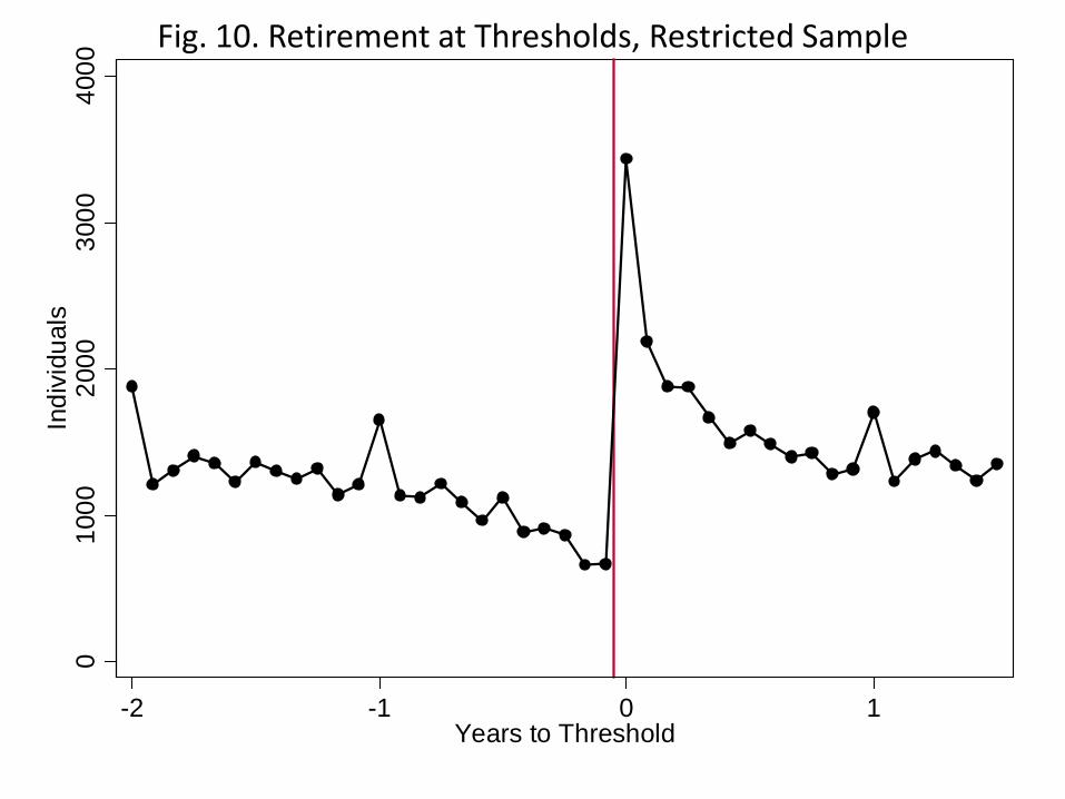
Given that Figures 7 through 9 demonstrate that there is heterogeneity in responsiveness

to the severance pay thresholds, we de�ne a restricted sample based on excluding the

least responsive or most constrained groups of individuals. The bottom panel in Table

1 summarizes the decreases in sample size resulting from excluding the least responsive

individuals along each dimension of heterogeneity that we have examined. The distribution

11

of tenure at retirement for the resulting sample of 154,484 individuals is shown in Figure

10. The basic patterns are the same as for the full sample.

Even in the restricted sample, we still observe several individuals retiring just prior to

the severance pay thresholds. However, eliminating the unresponsive groups does reduce the

probability of retirement shortly before the thresholds. In the full sample, the probability

of retiring in a quarter within 1 year before a threshold is 22% lower than the probability of

retiring in any other quarter. Each sample cut further lowers this probability so that in the

restricted sample, the probability of retiring in a quarter within 1 year before a threshold

is 29% lower than the probability of retiring in any other quarter.13

4 Theoretical Background

4.1 Preliminaries

We use the empirical evidence from the previous section to guide us in modeling la-

bor supply responses to the severance payments. First, the empirical evidence indicates

that individuals do not time their job starts earlier in their careers to be eligible for sev-

erance pay at the minimum retirement ages mandated by the government pension system.

Therefore, we focus only on the e¤ects of the severance payments on retirement decisions.

Second, given the lack of long-term planning in relation to the severance payments and

the relatively short time-space over which retirements takes place in Austria, the empiri-

cal evidence suggests that individuals�retirement decisions take into account at most one

tenure threshold when deciding when to retire. We therefore model the decision to delay

retirement based on the nearest, upcoming tenure threshold. Third, we �nd no evidence for

income e¤ects in the retirement patterns. Intuitively, the severance payments are small rel-

ative to lifetime income, and individuals may be unlikely to respond to such small changes

in lifetime income. The lack of evidence for income e¤ects guides the choice of the prefer-

ence speci�cation that we use below. For simplicity, we assume a preference speci�cation

that implies there are no income e¤ects in individuals�retirement decisions. Lastly, the

empirical evidence from the previous section indicates that, controlling for age and other

observable covariates does not alter the observed retirement patterns. This suggests that

tenure at age 55 is randomly distributed across individuals. As a consequence, we assume

13Results from linear probability models of the retirement indicator by quarter on a pre-threshold dummyand basic controls for gender, age, season, and a set of threshold indicators for di¤erent subsamples areavailable on request.

12

that the age or date until which each individual would need to work to reach the next

severance pay threshold is varying exogenously across individuals.

In summary, the empirical evidence suggests a basic decision rule capturing labor supply

responses to the severance payments. The decision rule is based a critical value that

captures the maximum length of time an individual would be willing to delay retirement

to qualify for a (larger) severance payment. An individual can determine how much he

would actually have to delay retirement by �rst selecting a retirement date neglecting the

severance payments and then determining how much additional tenure he would have to

accumulate to reach the next severance pay threshold. In this scenario, the decision rule is

the following: if the determined length of delay is less than the critical value, the individual

will delay and retire at the tenure threshold; otherwise, the individual will retire at the

date selected in the absence of the severance pay incentives.

This decision rule relates to a model of retirement decisions that can be exploited to

relate the observed retirement patterns to an intertemporal labor supply elasticity. Specif-

ically, the model highlights that, by focusing on an individual who is indi¤erent between

retiring at an early date without severance pay and retiring later with severance pay, the

implied indi¤erence condition can be used to get at the curvature in the disutility of work.

This curvature re�ects the intertemporal labor supply elasticity. Therefore, an important

identifying assumption in the estimation strategy will be that we can identify an individual

at the point of indi¤erence.

Before developing a model behind this decision rule, we recognize a potential concern

relating to predicted gaps in the distribution of tenure at retirement. Speci�cally, if the

above decision rule and the model behind it are applied to individuals with identical critical

values, we would predict that no one retires just prior to a severance pay threshold but that

there are gaps in the distribution of tenure at retirement just prior to the tenure thresholds.

While the empirical frequencies do decline prior to the tenure thresholds, we do not observe

any gaps in the distribution. We therefore interpret the decision rule and the model behind

it as applying to individuals who can respond to the severance payments. Other individuals

may not be able to respond to the severance payments and hence may retire just prior

to the tenure thresholds. We discuss factors that may account for these pre-threshold

retirements in more detail below. Importantly, individuals who are not responding to the

severance payments cannot be used to identify the intertemporal labor supply elasticity.

Following the estimation strategy that we develop below, we emphasize that we estimate

the intertemporal labor supply elasticity using only individuals that do respond to the

13

severance payments.

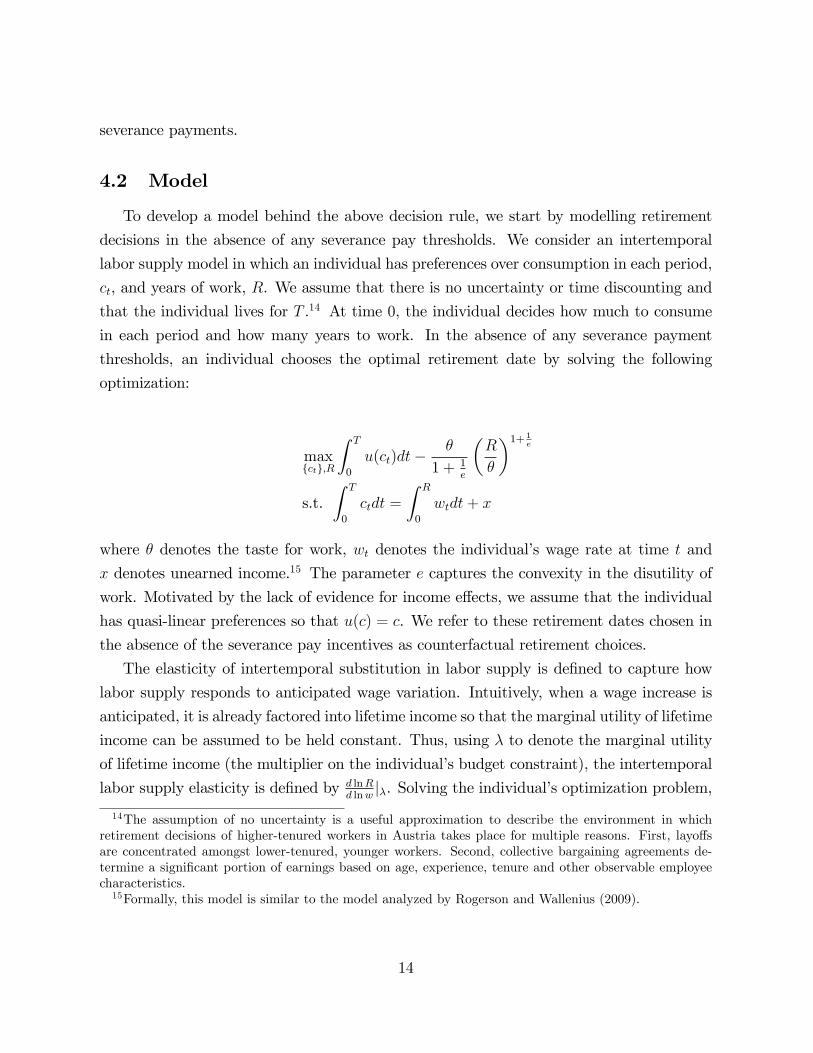
4.2 Model

To develop a model behind the above decision rule, we start by modelling retirement

decisions in the absence of any severance pay thresholds. We consider an intertemporal

labor supply model in which an individual has preferences over consumption in each period,

ct, and years of work, R. We assume that there is no uncertainty or time discounting and

that the individual lives for T .14 At time 0, the individual decides how much to consume

in each period and how many years to work. In the absence of any severance payment

thresholds, an individual chooses the optimal retirement date by solving the following

optimization:

maxfctg;R

Z T

0

u(ct)dt��

1 + 1e

�R

�

�1+ 1e

s.t.Z T

0

ctdt =

Z R

0

wtdt+ x

where � denotes the taste for work, wt denotes the individual�s wage rate at time t and

x denotes unearned income.15 The parameter e captures the convexity in the disutility of

work. Motivated by the lack of evidence for income e¤ects, we assume that the individual

has quasi-linear preferences so that u(c) = c. We refer to these retirement dates chosen in

the absence of the severance pay incentives as counterfactual retirement choices.

The elasticity of intertemporal substitution in labor supply is de�ned to capture how

labor supply responds to anticipated wage variation. Intuitively, when a wage increase is

anticipated, it is already factored into lifetime income so that the marginal utility of lifetime

income can be assumed to be held constant. Thus, using � to denote the marginal utility

of lifetime income (the multiplier on the individual�s budget constraint), the intertemporal

labor supply elasticity is de�ned by d lnRd lnw

j�. Solving the individual�s optimization problem,14The assumption of no uncertainty is a useful approximation to describe the environment in which

retirement decisions of higher-tenured workers in Austria takes place for multiple reasons. First, layo¤sare concentrated amongst lower-tenured, younger workers. Second, collective bargaining agreements de-termine a signi�cant portion of earnings based on age, experience, tenure and other observable employeecharacteristics.15Formally, this model is similar to the model analyzed by Rogerson and Wallenius (2009).

14

the intertemporal labor supply elasticity in this model is given by

d lnR

d lnwj� = e:

Intuitively, when the marginal disutility from additional labor supply rises very rapidly, an

individual will not adjust his labor supply very much in response to an anticipated wage

increase. In this model without income e¤ects, the intertemporal labor supply elasticity is

re�ected in the curvature in an individual�s indi¤erence curves.16,17

Next, we introduce the severance payments. We assume that each individual has a

threshold retirement date, denoted by �R, such that, when retiring after the threshold

date, the individual receives a lump-sum payment denoted by dx. Following the empirical

evidence, we assume that these threshold dates are randomly distributed across individuals.

As a result, the amount of time between an individual�s counterfactual retirement date and

his threshold date, denoted by dR = �R�R, varies across individuals. Optimal retirementchoices with the severance payments are presented graphically in Figure 11.

With the severance payments, several individuals will choose to delay their counterfac-

tual retirements and retire at the thresholds. In particular, given the �nancial incentives,

individuals who need to delay their counterfactual retirements by only a relatively small

amount of time will choose to retire at the thresholds. The set of individuals who delay

their retirements and pool at the tenure threshold is given by individuals with dR 2 [0;�]where � denotes the critical value capturing the maximum length of time an individual

is willing to delay his retirement to reach the tenure threshold. This critical value is de-

termined by solving for the length of time that makes an individual indi¤erent between

retiring early without the severance payment and retiring at the tenure threshold with the

severance payment. Using the optimization problem from above, � is characterized by

16In this setting, the intertemporal (Frisch) labor supply elasticity coincides with the static income-constant (Marshallian) and utility-constant (Hicksian) labor supply elasticities. Though they are concep-tually distinct, these labor supply elasticities coincide in this setting because there are no income e¤ectsby assumption (see Browning (2005)). Nonetheless, we refer to e as an intertemporal elasticity becausethe variation that will be used to identify and estimate this parameter will correspond to anticipated,within-person variation in wage rates over time periods.17We assume that the intertemporal labor supply elasticity e is homogeneous across individuals. We do

not see su¢ cient empirical evidence suggesting that this is a poor assumption. Additionally, we do nothave su¢ cient moments in the data to identify heterogeneous labor supply elasticities across individuals.We have estimated separate elasticities across each of the separate tenure thresholds and obtained resultssimilar to those presented below.

15

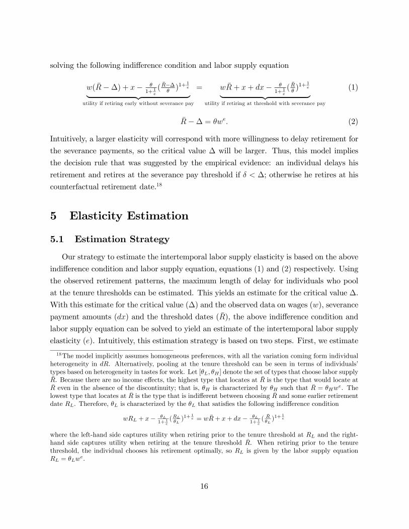
solving the following indi¤erence condition and labor supply equation

w( �R��) + x� �1+ 1

e

(�R���)1+

1e| {z }

utility if retiring early without severance pay

= w �R + x+ dx� �1+ 1

e

(�R�)1+

1e| {z }

utility if retiring at threshold with severance pay

(1)

�R�� = �we: (2)

Intuitively, a larger elasticity will correspond with more willingness to delay retirement for

the severance payments, so the critical value � will be larger. Thus, this model implies

the decision rule that was suggested by the empirical evidence: an individual delays his

retirement and retires at the severance pay threshold if � < �; otherwise he retires at his

counterfactual retirement date.18

5 Elasticity Estimation

5.1 Estimation Strategy

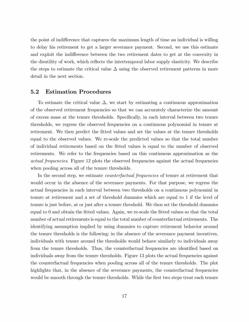
Our strategy to estimate the intertemporal labor supply elasticity is based on the above

indi¤erence condition and labor supply equation, equations (1) and (2) respectively. Using

the observed retirement patterns, the maximum length of delay for individuals who pool

at the tenure thresholds can be estimated. This yields an estimate for the critical value �.

With this estimate for the critical value (�) and the observed data on wages (w), severance

payment amounts (dx) and the threshold dates ( �R), the above indi¤erence condition and

labor supply equation can be solved to yield an estimate of the intertemporal labor supply

elasticity (e). Intuitively, this estimation strategy is based on two steps. First, we estimate

18The model implicitly assumes homogeneous preferences, with all the variation coming form individualheterogeneity in dR. Alternatively, pooling at the tenure threshold can be seen in terms of individuals�types based on heterogeneity in tastes for work. Let [�L; �H ] denote the set of types that choose labor supply�R. Because there are no income e¤ects, the highest type that locates at �R is the type that would locate at�R even in the absence of the discontinuity; that is, �H is characterized by �H such that �R = �Hwe. Thelowest type that locates at �R is the type that is indi¤erent between choosing �R and some earlier retirementdate RL. Therefore, �L is characterized by the �L that satis�es the following indi¤erence condition

wRL + x� �L1+ 1

e

(RL

�L)1+

1e = w �R+ x+ dx� �L

1+ 1e

(�R�L)1+

1e

where the left-hand side captures utility when retiring prior to the tenure threshold at RL and the right-hand side captures utility when retiring at the tenure threshold �R. When retiring prior to the tenurethreshold, the individual chooses his retirement optimally, so RL is given by the labor supply equationRL = �Lw

e.

16

the point of indi¤erence that captures the maximum length of time an individual is willing

to delay his retirement to get a larger severance payment. Second, we use this estimate

and exploit the indi¤erence between the two retirement dates to get at the convexity in

the disutility of work, which re�ects the intertemporal labor supply elasticity. We describe

the steps to estimate the critical value � using the observed retirement patterns in more

detail in the next section.

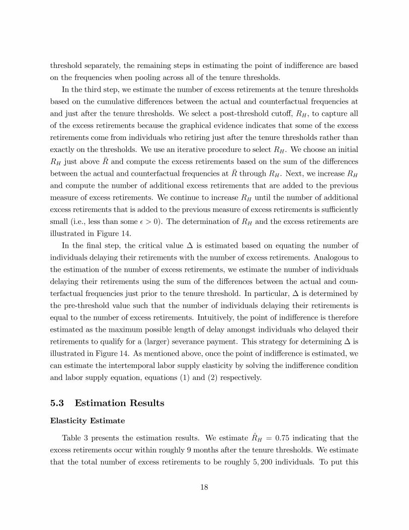
5.2 Estimation Procedures

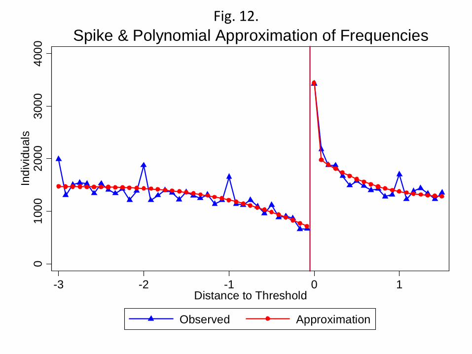
To estimate the critical value �, we start by estimating a continuous approximation

of the observed retirement frequencies so that we can accurately characterize the amount

of excess mass at the tenure thresholds. Speci�cally, in each interval between two tenure

thresholds, we regress the observed frequencies on a continuous polynomial in tenure at

retirement. We then predict the �tted values and set the values at the tenure thresholds

equal to the observed values. We re-scale the predicted values so that the total number

of individual retirements based on the �tted values is equal to the number of observed

retirements. We refer to the frequencies based on this continuous approximation as the

actual frequencies. Figure 12 plots the observed frequencies against the actual frequencies

when pooling across all of the tenure thresholds.

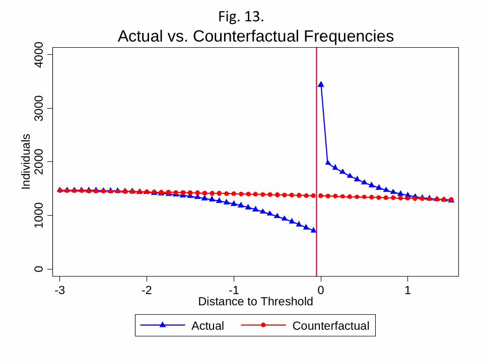
In the second step, we estimate counterfactual frequencies of tenure at retirement that

would occur in the absence of the severance payments. For that purpose, we regress the

actual frequencies in each interval between two thresholds on a continuous polynomial in

tenure at retirement and a set of threshold dummies which are equal to 1 if the level of

tenure is just before, at or just after a tenure threshold. We then set the threshold dummies

equal to 0 and obtain the �tted values. Again, we re-scale the �tted values so that the total

number of actual retirements is equal to the total number of counterfactual retirements. The

identifying assumption implied by using dummies to capture retirement behavior around

the tenure thresholds is the following: in the absence of the severance payment incentives,

individuals with tenure around the thresholds would behave similarly to individuals away

from the tenure thresholds. Thus, the counterfactual frequencies are identi�ed based on

individuals away from the tenure thresholds. Figure 13 plots the actual frequencies against

the counterfactual frequencies when pooling across all of the tenure thresholds. The plot

highlights that, in the absence of the severance payments, the counterfactual frequencies

would be smooth through the tenure thresholds. While the �rst two steps treat each tenure

17

threshold separately, the remaining steps in estimating the point of indi¤erence are based

on the frequencies when pooling across all of the tenure thresholds.

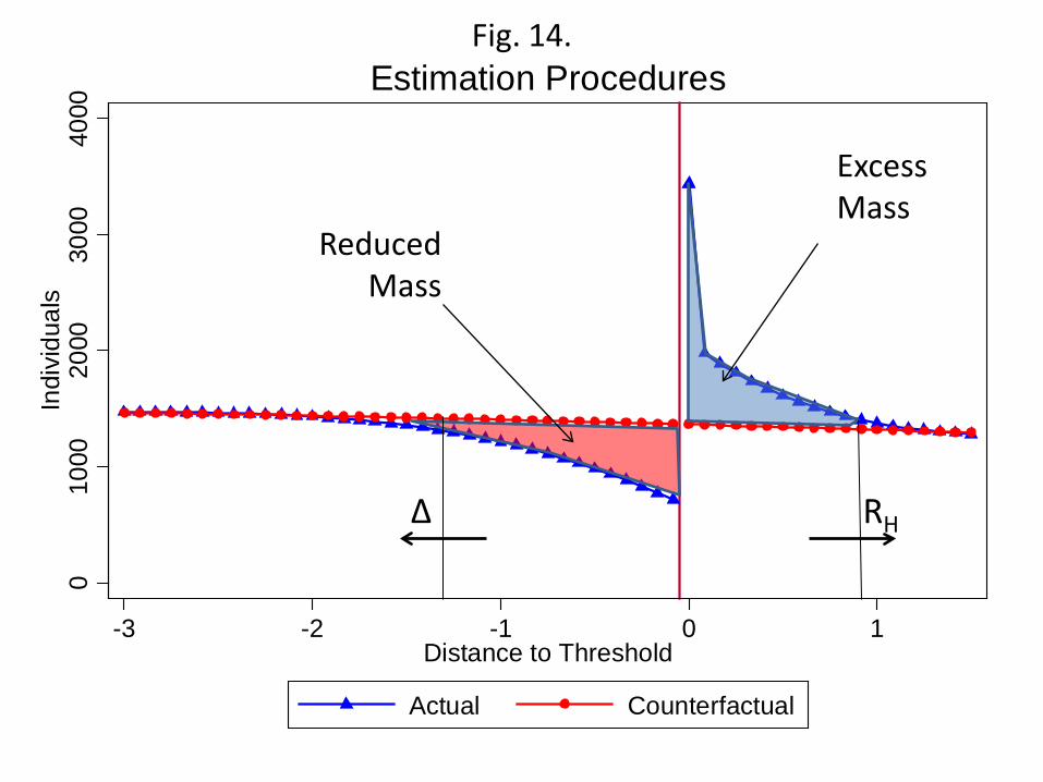
In the third step, we estimate the number of excess retirements at the tenure thresholds

based on the cumulative di¤erences between the actual and counterfactual frequencies at

and just after the tenure thresholds. We select a post-threshold cuto¤, RH , to capture all

of the excess retirements because the graphical evidence indicates that some of the excess

retirements come from individuals who retiring just after the tenure thresholds rather than

exactly on the thresholds. We use an iterative procedure to select RH . We choose an initial

RH just above �R and compute the excess retirements based on the sum of the di¤erences

between the actual and counterfactual frequencies at �R through RH . Next, we increase RHand compute the number of additional excess retirements that are added to the previous

measure of excess retirements. We continue to increase RH until the number of additional

excess retirements that is added to the previous measure of excess retirements is su¢ ciently

small (i.e., less than some � > 0). The determination of RH and the excess retirements are

illustrated in Figure 14.

In the �nal step, the critical value � is estimated based on equating the number of

individuals delaying their retirements with the number of excess retirements. Analogous to

the estimation of the number of excess retirements, we estimate the number of individuals

delaying their retirements using the sum of the di¤erences between the actual and coun-

terfactual frequencies just prior to the tenure threshold. In particular, � is determined by

the pre-threshold value such that the number of individuals delaying their retirements is

equal to the number of excess retirements. Intuitively, the point of indi¤erence is therefore

estimated as the maximum possible length of delay amongst individuals who delayed their

retirements to qualify for a (larger) severance payment. This strategy for determining � is

illustrated in Figure 14. As mentioned above, once the point of indi¤erence is estimated, we

can estimate the intertemporal labor supply elasticity by solving the indi¤erence condition

and labor supply equation, equations (1) and (2) respectively.

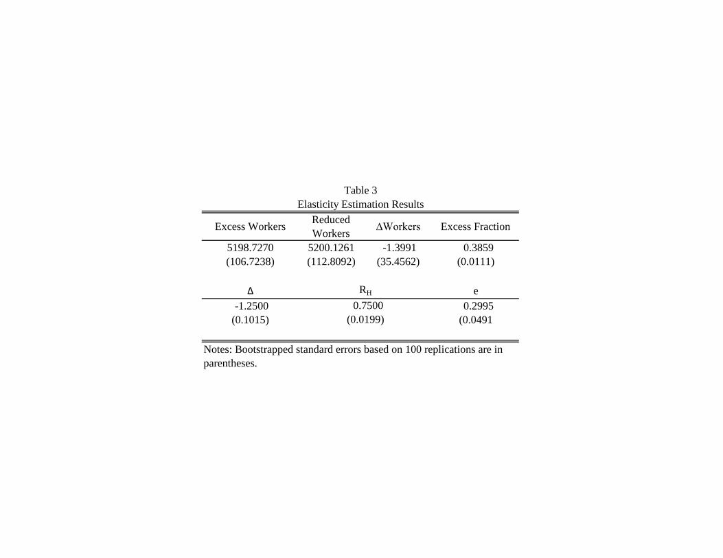
5.3 Estimation Results

Elasticity Estimate

Table 3 presents the estimation results. We estimate RH = 0:75 indicating that the

excess retirements occur within roughly 9 months after the tenure thresholds. We estimate

that the total number of excess retirements to be roughly 5; 200 individuals. To put this

18

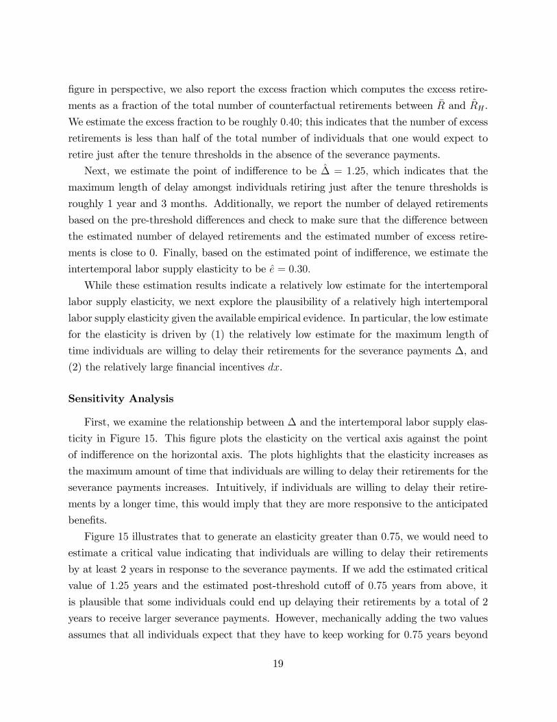
�gure in perspective, we also report the excess fraction which computes the excess retire-

ments as a fraction of the total number of counterfactual retirements between �R and RH .

We estimate the excess fraction to be roughly 0:40; this indicates that the number of excess

retirements is less than half of the total number of individuals that one would expect to

retire just after the tenure thresholds in the absence of the severance payments.

Next, we estimate the point of indi¤erence to be � = 1:25; which indicates that the

maximum length of delay amongst individuals retiring just after the tenure thresholds is

roughly 1 year and 3 months. Additionally, we report the number of delayed retirements

based on the pre-threshold di¤erences and check to make sure that the di¤erence between

the estimated number of delayed retirements and the estimated number of excess retire-

ments is close to 0. Finally, based on the estimated point of indi¤erence, we estimate the

intertemporal labor supply elasticity to be e = 0:30:

While these estimation results indicate a relatively low estimate for the intertemporal

labor supply elasticity, we next explore the plausibility of a relatively high intertemporal

labor supply elasticity given the available empirical evidence. In particular, the low estimate

for the elasticity is driven by (1) the relatively low estimate for the maximum length of

time individuals are willing to delay their retirements for the severance payments �, and

(2) the relatively large �nancial incentives dx.

Sensitivity Analysis

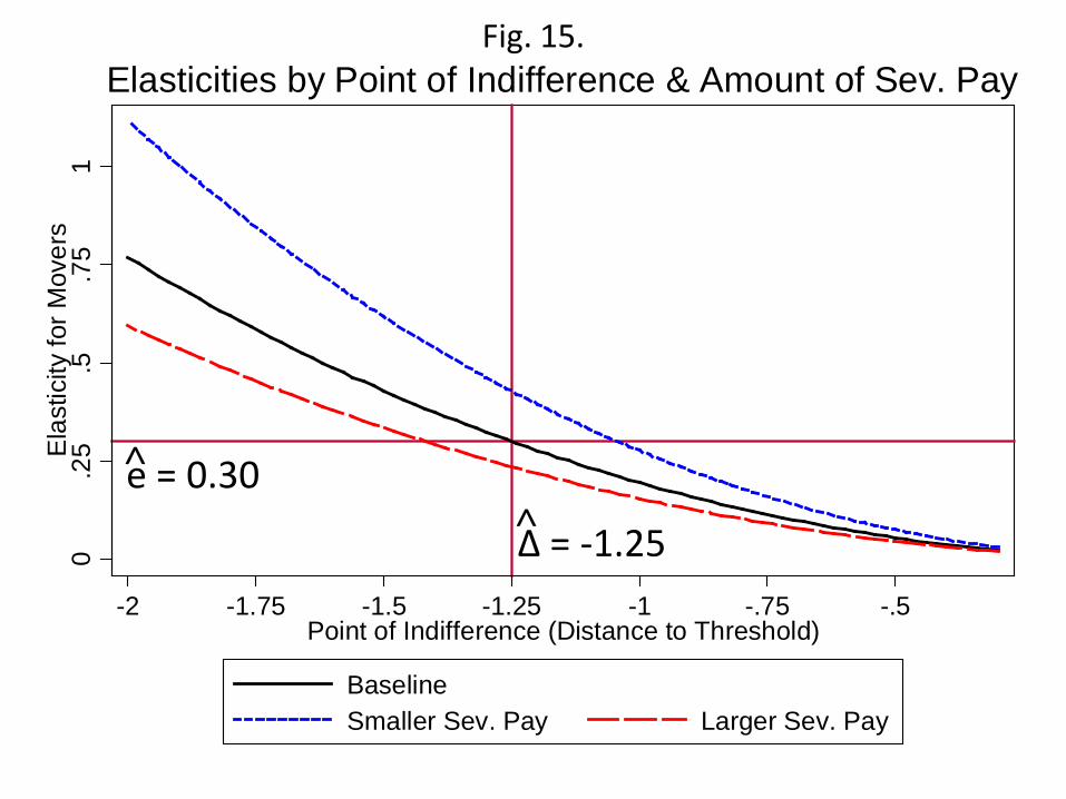
First, we examine the relationship between � and the intertemporal labor supply elas-

ticity in Figure 15. This �gure plots the elasticity on the vertical axis against the point

of indi¤erence on the horizontal axis. The plots highlights that the elasticity increases as

the maximum amount of time that individuals are willing to delay their retirements for the

severance payments increases. Intuitively, if individuals are willing to delay their retire-

ments by a longer time, this would imply that they are more responsive to the anticipated

bene�ts.

Figure 15 illustrates that to generate an elasticity greater than 0:75, we would need to

estimate a critical value indicating that individuals are willing to delay their retirements

by at least 2 years in response to the severance payments. If we add the estimated critical

value of 1:25 years and the estimated post-threshold cuto¤ of 0:75 years from above, it

is plausible that some individuals could end up delaying their retirements by a total of 2

years to receive larger severance payments. However, mechanically adding the two values

assumes that all individuals expect that they have to keep working for 0:75 years beyond

19

their threshold dates. We observe that individuals who pool at the tenure thresholds

generally retire within a few weeks of the thresholds, which does not seem to be much

evidence to justify such an assumption. Overall, we do not �nd much evidence suggesting

that individuals who pool at the tenure thresholds are willing to delay their retirements by

2 years or more to qualify for the larger severance payments.

Second, we examine the relationship between the �nancial incentives from the severance

payments and the estimated intertemporal labor supply elasticity. Figure 15 plots the

implied intertemporal labor supply elasticity against the point of indi¤erence if the size

of the discontinuity in the budget line were either 33% larger and 33% smaller than the

mandated amount. Intuitively, at each point of indi¤erence, a smaller discontinuity implies

a larger elasticity because individuals are similarly responsive to smaller �nancial incentives.

Based on the the estimated point of indi¤erence of 1:25 year before the tenure thresholds,

a 33% smaller discontinuity would results in an estimated elasticity of roughly 0:40.

Uncertainty is one factor that could potentially reduce individuals��nancial incentives

to delay their retirements. To see this, consider the model above and suppose that an

individual gets the severance payment dx at the threshold �R with probability p 2 (0; 1),and with probability 1 � p, the individual is forced to retire at some other date not ofhis choice and he does not receive a payment. Intuitively, such uncertainty could arise

from either a health shock or a layo¤. Additionally, if an employer o¤ers early severance

payments and tries to force some fraction of his employees to retire, this could be modeled

similarly. In this scenario, the �nancial incentives to delay retirement are reduced to

pdx. As indicated by Figure 15, the probability p would need to be smaller that 0:66 to

generate an elasticity larger than 0:40. To generate a larger intertemporal labor supply

elasticity, one would need to assume a signi�cant amount of uncertainty in getting the

severance payments at the tenure thresholds because the direct �nancial incentives from

the payments are relatively large. The empirical evidence on health shocks and layo¤s at

older ages indicates a relatively low degree of uncertainty. Thus, there seems to be little

empirical evidence suggesting that the �nancial incentives from the severance payments

actually small enough to generate a relatively high estimate for the intertemporal labor

supply elasticity.

20

5.4 Model Simulations

While the model and estimation focus on individuals who can choose to delay their

retirements to respond to the severance payments, we now present model simulations to

examine features that can account for individuals retiring just before the tenure thresholds

and slightly after the tenure thresholds.

To account for the pre-threshold retirements, we introduce a health cost associated with

the additional work when delaying one�s retirement beyond a counterfactual date without

the severance payments. We assume that an individual who determines the utility gain

dU from delaying retirement to the threshold date also draws a health cost � capturing an

exogenously given additional marginal disutility of work from delaying his retirement (� >

0). After comparing utility gain and the health cost, individuals delay their retirements if

the amount of additional work is su¢ ciently low (i.e. dR < �) and also if their utility gains

exceed their health costs (i.e. dU > �). We assume that the health costs are independent

draws from a random distribution. Hence, the probability of delaying retirement increases

from close to 0 for a length of delay equal to the maximum length dR = � to a fraction m

for a length of delay dR close to 0; in other words, the probability of delaying retirement is

higher if an individual has to delay his retirement by only a relatively small amount of time.

We determine m based on the actual number of pre-threshold retirements as a fraction of

the counterfactual pre-thresholds retirements.

To account for the retirements slightly after the tenure thresholds, we introduce task

completion constraints as additional noise added to individuals�optimal retirement dates.

Speci�cally, we assume that, once an individual has chosen to retire at a tenure threshold,

he draws a task that he must complete prior to retirement. The observed retirement

date then becomes ~R = �R+ z where z captures the amount of time taken to complete the

task. We assume that z is drawn from an exponential distribution with parameter �task > 0

capturing the average amount of additional time taken for task completion. This parameter

is calibrated based on the excess retirements observed just after the tenure thresholds.19

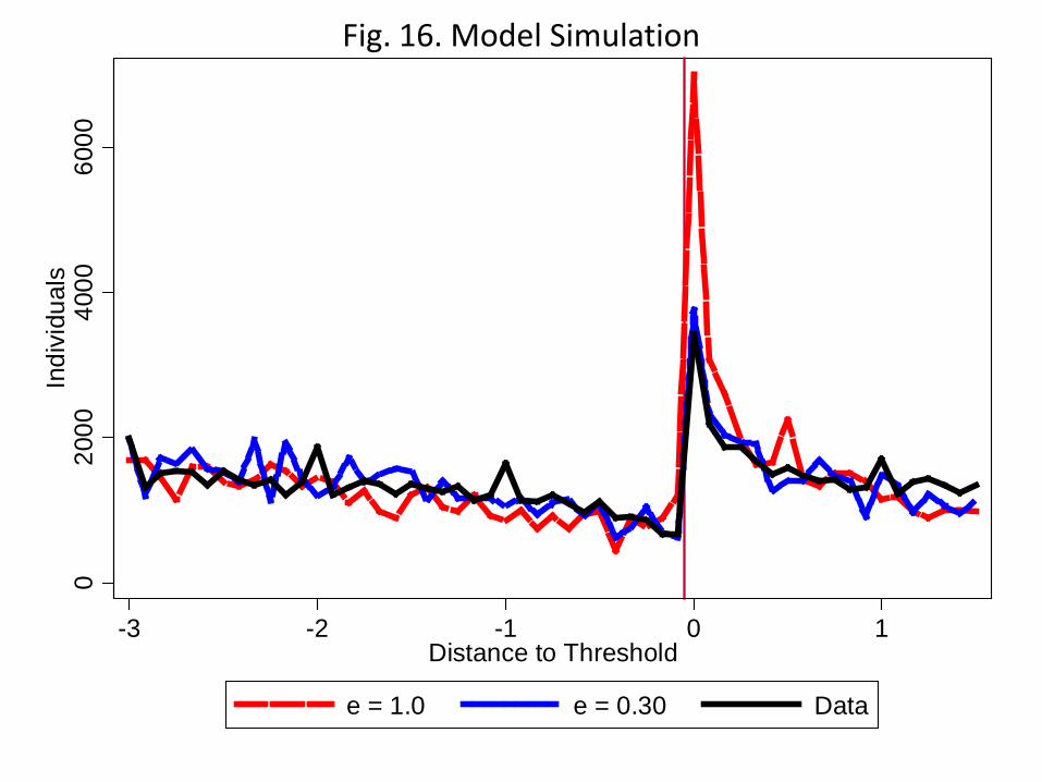
Figure 16 plots the observed data against the simulated outcomes from the model with

the health costs and task completion constraints. In this simulation, we use an elasticity of

0:30 and calibrate the parameter values for the health costs and task constraints to match

the observed data. The �gure highlights that the model is able to replicate the observed pre-

and post-threshold patterns after introducing the health costs and task completion frictions.

19For simplicity we assume that task completion frictions only occur if an individual decides to retire atthe tenure threshold. If we added the constraint to all retirements nothing would change??

21

Next, we examine the simulated patterns when using a relatively high intertemporal labor

supply elasticity of 1:0 and the same parameter values for the costs and constraints. In this

case, the simulated number of excess retirements is much larger than the observed number

of excess retirements.20 Intuitively, a relatively high intertemporal labor supply elasticity

would imply many more excess retirements at the tenure thresholds than we can detect

from the observed data. Overall, we �nd little evidence for a relatively high intertemporal

labor supply elasticity.

6 Conclusions

This paper presents evidence on individuals�willingness to delay exiting the labor force

in response to anticipated increases in retirement bene�ts. This evidence is based on

discontinuous increases in retirement bene�ts upon completion of 10, 15, 20, and 25 years

of tenure by retirement. The graphical evidence illustrates a relatively modest willingness

to delay retirement in response to the discontinuous increases in bene�ts at the tenure

thresholds. This evidence implies a low intertemporal labor supply elasticity of 0:30. Thus,

either based on intensive or extensive margin labor supply decisions, economic models that

rely on high intertemporal labor supply elasticities appear to be at odds with available

empirical evidence.

20Importantly, this simulation is done using the cost and friction parameters calibrated using the elasticityof 0:30. Alternatively, one could calibrate these parameters when using the observed data and an elasticityof 1:0 and then examine how the excess mass just after the tenure thresholds changes when using a lowerlabor supply elasticity. However, in this case, the excess number of retirements is not responsive to thechange in the labor supply elasticity because the simulated excess retirements are driven almost entirely bythe costs and frictions. Intuitively, the intertemporal labor supply elasticity is not identi�ed if the observedpatterns are driven entirely by randomly drawn costs and frictions rather than by individuals choosingtheir retirements in the presence of relatively small frictions.

22

References

Blundell, R. and T. Macurdy (1999). Labor supply: A review of alternative approaches.

In O. Ashenfelter and D. Card (Eds.), Handbook of Labor Economics, Volume 3 of

Handbook of Labor Economics, Chapter 27, pp. 1559�1695. Elsevier.

Card, D., R. Chetty, and A. Weber (2007). Cash-on-Hand and Competing Models of

Intertemporal Behavior: New Evidence from the Labor Market. Quarterly Journal

of Economics 122 (4), 1511�1560.

Chetty, R., J. N. Friedman, T. Olsen, and L. Pistaferri (2009). Adjustment costs, �rm

responses, and labor supply elasticities: Evidence from danish tax records. Working

Paper 15617, National Bureau of Economic Research.

Heckman, J. J. (1993). What has been learned about labor supply in the past twenty

years? American Economic Review 83 (2), 116�121.

Keane, M. and R. Rogerson (2010). Reconciling micro and macro labor supply elasticities.

Working paper.

Ljungqvist, L. and T. Sargent (2010). Career length: E¤ects of curvature of earnings

pro�les, earnings shocks, and social security. Working paper.

Ljungqvist, L., T. J. Sargent, O. Blanchard, and E. C. Prescott (2006). Do Taxes Explain

European Employment? Indivisible Labor, Human Capital, Lotteries, and Savings

[with Comments and Discussion]. NBER Macroeconomics Annual 21, 181�246.

Mulligan, C. B. (1999). Substition over time: Another look at life-cycle labor supply.

In B. Bernanke and J. Rotemberg (Eds.), NBER Macroeconomics Annual 1998, Vol-

ume 13, pp. 75�152. MIT Press.

Ohanian, L., A. Ra¤o, and R. Rogerson (2008). Long-term Changes in Labor Supply

and Taxes: Evidence from OECD Countries, 1956-2004. Journal of Monetary Eco-

nomics 55 (8), 1353�1362.

Prescott, E. C. (2006). Nobel Lecture: The Transformation of Macroeconomic Policy

and Research. Journal of Political Economy 114 (2), 203�235.

Saez, E. (1999). Do taxpayers bunch at kink points? Working Paper 7366, National

Bureau of Economic Research.

Saez, E. (2010). Do taxpayers bunch at kink points? American Economic Journal:

Economic Policy (forthcoming).

23

Zweimüller, J., R. Winter-Ebmer, R. Lalive, A. Kuhn, J.-P. Wuellrich, O. Ruf, and

S. Büchi (2009). Austrian social security database. NRN: The Austrian Center for

Labor Economics and the Analysis of the Welfare State (Working Paper 0903).

24

Number of Observations

Percentage change

Individuals in cohorts born 1930 - 1940 1,578,549Still employed at age 55 651,336 -59%More than one year employment experience before age 55 625,251 -4%Excluding workers ever employed as civil servant 546,308 -13%Excluding workers withlast job not in construction 487,019 -11%Excluding left censored tenure in last job 380,737 -22%Workers retiring withing 6 months of their last job 269,411 -29%

Restricted sample of highly responsive individualsExcluding individuals with high number of sick leave days 233,976 -13%Excluding individuals with high or low average earnings 197,726 -15%Excluding workers from firms with less than 10 employees 159,186 -19%Excluding workers with in jobs with highest rigidity index 154,484 -3%Notes: Numbers based on the ASSD

Table 1Sample Selection

Full Sample Tenure at Retirement ≥ 10

# of Individuals 269,411 142,332

Retirement Age 58.64 58.7159.00 59.252.58 2.61

Tenure 11.11 17.2710.50 16.507.76 5.06

Annual Earnings 18459.69 19572.4817983.05 19649.5213458.51 13571.58

Fraction Top-Coded 0.14 0.15- -

0.34 0.36

Years of Employment 32.71 34.0834.54 35.289.59 8.36

Years of Sick Leave 0.48 0.430.12 0.090.88 0.81

Fractions:Claiming Disability Pensions 0.282 0.233Claiming Early Retirement Pensions 0.375 0.401Claiming Old Age Pensions 0.343 0.366

Agriculture & Mining 0.045 0.041Manufacturing 0.255 0.240Sales 0.193 0.167Tourism 0.044 0.022Transportation 0.051 0.045Services 0.412 0.485

Notes: Except for the Fractions, the mean, median and standard deviations are reported for each variable. All earnings variables are expressed in 2008 euros. Summary statistics for lifetime earnings are based on birth cohorts beyond 1935. Employment Time and Sick Leave are measured in years.

Summary Statistics Table 2

Excess Workers Reduced Workers ∆Workers Excess Fraction

5198.7270 5200.1261 -1.3991 0.3859(106.7238) (112.8092) (35.4562) (0.0111)

Δ e -1.2500 0.2995(0.1015) (0.0491

Notes: Bootstrapped standard errors based on 100 replications are in parentheses.

Table 3Elasticity Estimation Results

RH

0.7500(0.0199)

0.3

33.5

.75

1Fr

actio

n of

Las

t Yea

r's S

alar

y

0 5 10 15 20 25 30Years of Tenure

Fig. 1. Payment Amounts based on Tenure at Retirement

0.2

.4.6

.81

Sur

vivo

r Fun

ctio

n

55 56 57 58 59 60 61 62 63 64 65 66 67 68 69 70Age

Men Women

Fig. 2. Exits from Labor Force into Retirement

050

010

0015

0020

00In

divi

dual

s

10 15 20 25Years of Tenure at Retirement

Fig. 3. Distribution of Tenure at Retirement, Full Sample

-.04

-.02

0.0

2.0

4R

egre

ssio

n C

oeffi

cien

t

10 15 20 25Years of Tenure at Retirement

Fig. 4. Controlling for Covariates

050

010

0015

0020

00#

of In

divi

dual

s S

tarti

ng N

ew J

obs

40 41 42 43 44 45 46 47 48 49 50 51 52 53 54 55 56 57 58 59 60Age

Women Men

Fig. 5. Job Starts by Age

050

010

0015

0020

00In

divi

dual

s

10 15 20 25Years of Tenure at Retirement

050

100

150

200

Indi

vidu

als

10 15 20 25Years of Tenure at Retirement

Fig. 6. Distribution of Tenure at Retirement by Health Status

Healthy

Unhealthy

200

300

400

500

600

700

Indi

vidu

als

-2 -1 0 1 2Years to Threshold

200

300

400

500

600

700

Indi

vidu

als

-2 -1 0 1 2Years to Threshold

200

300

400

500

600

700

Indi

vidu

als

-2 -1 0 1 2Years to Threshold

200

300

400

500

600

700

Indi

vidu

als

-2 -1 0 1 2Years to Threshold

Fig. 7. Retirement at Thresholds by Earnings Groups

21st-25th

percentiles56th-50th

percentiles

71st-75th

percentiles>95th

percentiles

020

040

060

0In

divi

dual

s

10 15 20 25Years of Tenure at Retirement

020

040

060

0In

divi

dual

s

10 15 20 25Years of Tenure at Retirement

020

040

060

0In

divi

dual

s

10 15 20 25Years of Tenure at Retirement

020

040

060

0In

divi

dual

s

10 15 20 25Years of Tenure at Retirement

Fig. 8. Distribution of Tenure at Retirement by Firm Size

Firm size: 150-499

Firm size: 50-149

Firm size: 10-49

Firm size: <10

100

200

300

400

Indi

vidu

als

-2 -1 0 1 2Years to Threshold

500

1000

1500

2000

Indi

vidu

als

-2 -1 0 1 2Years to Threshold

2000

4000

6000

8000

Indi

vidu

als

-2 -1 0 1 2Years to Threshold

Fig. 9. Retirement at Thresholds by Job Rigidity

High Rigidity Medium Rigidity

Low Rigidity

010

0020

0030

0040

00In

divi

dual

s

-2 -1 0 1Years to Threshold

Fig. 10. Retirement at Thresholds, Restricted Sample

Labor Supply

€

RcloseR

dx

Fig. 11. Optimal Retirement Choices with Severance Pay

Rindifferent

Point of Indifference (Max Length of Delay) :Δ = Rindifferent – R

Rfar

010

0020

0030

0040

00In

divi

dual

s

-3 -2 -1 0 1Distance to Threshold

Observed Approximation

Spike & Polynomial Approximation of FrequenciesFig. 12.

010

0020

0030

0040

00In

divi

dual

s

-3 -2 -1 0 1Distance to Threshold

Actual Counterfactual

Actual vs. Counterfactual FrequenciesFig. 13.

010

0020

0030

0040

00In

divi

dual

s

-3 -2 -1 0 1Distance to Threshold

Actual Counterfactual

Estimation Procedures

Excess Mass

Reduced Mass

Δ RH

Fig. 14.

0.2

5.5

.75

1E

last

icity

for M

over

s

-2 -1.75 -1.5 -1.25 -1 -.75 -.5Point of Indifference (Distance to Threshold)

BaselineSmaller Sev. Pay Larger Sev. Pay

Elasticities by Point of Indifference & Amount of Sev. Pay

e = 0.30

Δ = -1.25

<

<

Fig. 15.

020

0040

0060

00In

divi

dual

s

-3 -2 -1 0 1Distance to Threshold

e = 1.0 e = 0.30 Data

Fig. 16. Model Simulation