Embed Size (px)
Citation preview
Intertemporal Substitutionin Labor Force Participation:
Evidence from Policy Discontinuities
Dayanand ManoliUCLA
Andrea WeberUniversity of Mannheim
April 28, 2010
Abstract
How much are individuals willing to reallocate labor supply from periods withlow wages to periods with high wages? We address this question using administrativedata on the census of private sector employees in Austria and variation from policydiscontinuities in retirement bene�ts from the Austrian pension system. The policydiscontinuities refer to discontinuous increases in bene�ts upon completion of 10, 15,20 or 25 years of tenure at retirement. We �rst present graphical evidence document-ing delays in retirement in response to the policy discontinuities. Next, we develop abasic model of retirement decisions and estimate the elasticity of intertemporal sub-stitution in labor force participation using a semiparametric estimator that exploitsthe graphical evidence. The graphical evidence and estimated elasticities indicate arelatively low degree of intertemporal substitution in labor force participation. Theseestimates have a high degree of precision due to both the minimal measurement er-ror and large sample size from the administrative data and also the large changes in�nancial incentives from the policy discontinuities.
1

1 Introduction
Understanding individuals�willingness to reallocate labor supply from times with low
wages to times with high wages is important for a variety of economic policies. However,
estimating the degree of intertemporal substitution in labor supply has proven di¢ cult
because of the research design that is required to estimate the elasticities and parameters
of interest. Ideally, to estimate the degree of intertemporal substitution in labor supply, one
requires a research design where identi�cation is based on exogenous variation in anticipated
wage changes across individuals. Previous studies have taken a variety of approaches to
simplify this research design, but the approaches have produced a wide range of estimates
with di¤erent policy implications.1
In this paper, we present new estimates of the degree of intertemporal substitution in
labor supply based on policy discontinuities in retirement bene�ts in Austria. We �rst
present graphical evidence documenting individuals�labor supply responses to the policy
discontinuities. Next, we develop a semiparametric elasticity estimator that exploits the
labor supply responses observed in the graphical evidence.
The policy discontinuities arise because retirement bene�ts in Austria vary discontinu-
ously based on the amount of tenure an individual has accumulated by his/her retirement.
Speci�cally, if an individual accumulates at least 10 years of tenure by retirement, the
Austrian pension system mandates that the employer must make a lump-sum payment to
the individual at the time of his/her retirement equal to one third of the last year�s salary.
If the individual accumulates less than 10 years of tenure by retirement, no payment is
made. If the individual accumulates at least 15, 20 or 25 years of tenure by retirement,
the payment amounts are increases to one half, three quarters and one full year of the last
year�s salary. These discontinuities therefore discontinuously increase wage rates just prior
to the thresholds. For example, the wage rate for the 10th year of tenure is discontinuously
higher than other years since individuals will receive their standard annual wage rate plus
the payment when they complete the 10th year. Furthermore, these wage increases can be
fully anticipated at earlier years of tenure.
We examine behavior before and after these tenure thresholds to determine if individ-1Microeconomic studies such as MaCurdy (1981), Altonji (1986), Blundell, Meghir and Neves (1993)
and Ziliak and Kniesner (1999) present evidence of relatively low intertemporal substitution in labor supply.In contrast, macroeconomic studies (see Mulligan (1999), King and Rebelo (1999) and Chang and Kim(2007)) have presented evidence of relatively high intertemporal substitution in labor supply. More recently,Looney and Singhal (2006) present microeconomic evidence of relatively high intertemporal substitutionin labor supply.
2

uals delay their retirements in response to the anticipated wage variation. The graphical
evidence indicates excess retirements just after the thresholds and reduced retirements just
prior to the thresholds. We then use a standard labor supply model to develop semipara-
metric estimator for the elasticity of intertemporal substitution in labor supply based on
the graphical evidence. While this estimator relies on discontinuities in individuals�bud-
get constraints, it is similar in spirit to previous bunching estimators that exploit kinks in
individuals�budget constraints (see Saez (1999, 2009) and Chetty et al (2009)).
Our research strategy contributes several innovations to the economics literature. First,
we contribute to the retirement literature by focusing explicitly on the elasticity of intertem-
poral substitution (i.e. the Frisch elasticity) in retirement decisions. Previous studies have
examined retirement responses to unanticipated changes in retirement bene�ts (for ex-
amples, see Krueger and Pischke (1992), Brown (2009) and Manoli, Mullen and Wagner
(2010)). However, since social security reforms are infrequent, it is important for policy-
makers to understand how retirement decisions respond to anticipated changes in retire-
ment bene�ts, and this exactly corresponds to understanding intertemporal substitution in
retirement decisions (see Browning (2005)).
Second, this research contributes to the labor economics and macroeconomics litera-
tures by focusing on an extensive margin Frisch elasticity. Many studies in both labor
economics and macroeconomics have emphasized the empirical relevance of the extensive
margin in the labor supply-wage relationship (see Heckman (1993) and Rogerson andWalle-
nius (2009)). However, previous microeconomics studies have generally presented evidence
of intertemporal substitution based on intensive margin labor supply changes.2 This study
presents microeconomic evidence of intertemporal substitution based on extensive margin
labor supply changes since retirement decisions are extensive margin decisions.
Finally, our empirical methodology presents multiple innovations to the literature on
retirement and intertemporal substitution in labor supply. While previous structural es-
timation strategies have often been forced to make speci�c distributional assumptions to
recover structural parameters, we are able to recover a policy-relevant structural parameter
from a quasi-experimental design without having to make these parametric assumptions.
Second, our empirical design allows for improvements to the estimates of intertemporal
substitution in the literature with regard to statistical and economic precision.. The gain
in statistical precision from our estimates follows from two factors. First, we are able to use
2See Blundell and MaCurdy (1999) for a survey of the microeconomic evidence of intertemporal substi-tution in labor supply.
3

administrative data from the Austrian Social Security Database, which minimizes measure-
ment error in key variables. Second, the data present a longitudinal census of private sector
employees and hence we have a large sample of 444,452 individuals. The economic precision
of our estimates arises from the magnitudes of the policy discontinuities. Previous studies
have exploited relatively small changes in �nancial incentives to examine intertemporal
substitution. If small optimization frictions (for example cognitive costs) exist, estimates
based on these small changes are unlikely to re�ect the structural parameter of interest
(see Chetty (2009)). In contrast, we exploit relatively large and transparent changes in
�nancial incentives of 400% of an individual�s monthly wage. Small optimization frictions
are less likely to overwhelm the large �nancial incentives thereby permitting more robust
or economically precise identi�cation of the structural parameter of interest.
This paper is organized as follows. Section 2 discusses both the institutional background
regarding the Austrian pension system and the administrative data from the Austrian
Social Security Database. We present the graphical evidence in section 3. We develop the
elasticity estimator and present the results in section 4. We discuss how alternative, more
complicated models would a¤ect the results in section 5 and we conclude in section 6.
2 Institutional Background & Data
2.1 Retirement Bene�ts in Austria
There are two forms of government mandated retirement bene�ts in Austria: (1)
government-provided pension bene�ts and (2) employer-provided severance payments. We
focus �rst on the severance payments since these payments are the primary focus of the
current study. The employer-provided severance payments are made to private sector em-
ployees who have accumulated su¢ cient years of tenure by the time of their retirement.3
Tenure is de�ned as continuous employment time with a given employer. Retirement is
based on claiming a government-provided pension as payments must be made within 4
weeks of claiming a pension. The payment schedule is as follows. If an employee has accu-
mulated 10 years of tenure with his employer by the time of his retirement, the employer
must pay the individual one third of his last year�s salary. This fraction increases from
3Severance payments are also made to individuals who are involuntarily separated (i.e. laid o¤) fromtheir �rms if the individuals have accumulated su¢ cient years of tenure prior to the separation. Theonly voluntary separation that leads to a severance payment is retirement. For more details regarding theseverance payments at times of unemployment, see Card, Chetty and Weber (2007).
4

one third to one half, three quarters and one at 15, 20 and 25 years of tenure respectively.
This schedule for the severance payments is illustrated in Figure 1. The payments are
must be made in lump-sum and, since payments are based on an employee�s salary, over-
time compensation and other non-salary payments are not included when determining the
amounts of the payments. Funds to make these payments come from funds that employers
are mandated to hold based on the total number of employees.
The Austrian income tax system, which is based on individual taxation, applies par-
ticular rules to tax income from severance payments. Speci�cally, all mandated severance
payments are exempt from social security contributions and subject to a tax rate of 6%.
The income taxation of the severance payments di¤ers from the general income tax rules.
Generally, gross monthly earnings net of social security contributions4 are subject to the
income tax with marginal tax rates in the di¤erent tax brackets of 0%, 21%, 31% 41% and
50%.5 Additionally, Austrian employees are typically paid 13th and 14th monthly wage
payments in June and December. These payments, up to an amount of one sixth of annual
wage income, are also subject to a 6% tax rate; amounts in excess of one sixth of annual
income are subject to the regular income tax rates.
Because the timing of the severance payments relates to pension claiming, eligibility
for government-provided retirement pensions interacts with the severance payment system.
Austria has a public pension system that automatically enrolls every person employed in
the private sector. Fixed pension contributions are withheld from each individual�s wage
and annuitized bene�ts during retirement are then based on prior contributions (earnings
histories). Replacement rates from the annual payments are roughly 75% of pre-retirement
earnings and there are no actuarial adjustments for delaying retirement to a later age.
Individuals can retire by claiming Disability pensions, Early Retirement pensions and Old
Age pensions. Eligibility for each of these pensions depends on an individual�s age and
gender, as well as having a su¢ cient number of contribution years. Beginning at age
55, private sector male and female employees can retire by claiming a Disability pension,
where disability is based on reduced working capacity of 50% relative to someone of a
similar educational background. At age 55, women also become eligible to claim Early
Retirement pensions, but this Early Retirement Age is age 60 for men. Lastly, men and
women become eligible for Old Age pensions at age 65 and 60 respectively.
4Contributions for pension, health, unemployment, and accident insurance of 39% are withheld fromgross annual earnings up to a contribution cap.
5These tax brackets are based on legislation in 2002; there have subsequently been relatively smallchanges due to several small tax reforms.
5
Figure 2 illustrates survival functions for entry into the pension system for the sample
of private sector employees. The survival functions are presented separately for men and
women given the separate eligibility ages. The survival functions illustrate sharp declines
at ages 60 and 65 highlighting a signi�cant amount of entry into the pension system once
individuals become eligible for the Early Retirement and Old-Age pensions. Additionally,
the �gure demonstrates that, for both men and women, most retirements occur between
ages 55 and 60. In particular, the survival function for men highlights that roughly 25% of
the sample of men retire by claiming disability pensions.
2.2 Administrative Data & Sample Restrictions
Our empirical analysis is based on data from the Austrian Social Security Database
(see Zweimuller et al (2009)), which are collected with the principle aim of verifying pen-
sion claims. This implies that the data provide very detailed longitudinal information on
employment and earnings for the universe of private sector workers in Austria. The period
for which registers are available spans the years 1972 to 2006. To investigate the e¤ect of
severance pay eligibility on retirement decisions we consider all individuals born between
1920 and 1945 and make several restrictions to the original dataset which are summarized
in Table A1 in the Appendix. Speci�cally, we focus on workers who are still employed
after their 55th birthday and follow them until entry into retirement or up to the age of
70. Because we are interested in tenure at the time of retirement, we only consider re-
tirement entries which occur within 6 months of the worker�s last job. Individuals with
longer gaps between employment and retirement are only followed until the end of the last
employment. Furthermore, because we want to ensure accurate computation of tenure at
retirement, we focus only on individuals with uncensored tenure at retirement. The cen-
soring arises for individuals that are continuously employed from the start of the data in
January of 1972 through their retirements. With these restrictions, we have a �nal sample
of 596; 897 individuals.
Table 1 presents some summary statistics for the �nal sample. Summary statistics are
presented for all individuals at age 55 and for all individuals at their retirement age if the
individual is observed to retire. Because of the imposed censoring at age 70 and the natural
censoring due to the end of the observation period in 2006, we observe 444; 452 retirements
out of the 596; 897 individuals observed at age 55. We present statistics of monthly earnings
since several individuals are observed to retire in the middle of a calendar year and thus
6

their annual earnings are reduced in the year of retirement. Median monthly earnings in the
month preceding retirement are roughly between 830 euros in 2004. Earnings increase with
age, so average and median earnings at retirement slightly exceed earnings their respective
counterparts at age 55. Average tenure at age 55 is relatively low (median of 4:75), but
the fraction of individuals eligible for severance payments increases as individuals age and
accumulate tenure. In particular, the median retirement age is roughly 4:75 years beyond
age 55 and the median tenure at retirement is about 3 years greater than tenure at age 55.
3 Nonparametric Analysis
3.1 Full Sample Analysis
3.1.1 Tenure at Retirement
Figure 3 presents the distribution of tenure at retirement for the full sample with the
number of individuals on the vertical axis and years of tenure at retirement on the hor-
izontal axis; tenure at retirement is measured at a monthly frequency. Several features
are evident from this plot. First, the plot shows discontinuous increases in the number
of retirements at and just beyond the tenure thresholds. Second, there are decreases in
the number of retirements just before the tenure thresholds. The observed decreases and
increases around the thresholds are generally concentrated within 1 year before and after
the thresholds respectively. These two patterns are not apparent at any other points in the
tenure distribution. This evidence suggests that individuals who would have retired just
before the thresholds in the absence of the severance pay discontinuities end up delaying
their retirements until they just qualify for the (larger) severance payments. Third, the
plot illustrates increases in the number of retirement at each integer value of tenure at
retirement. This seasonality is driven by several jobs beginning on January 1st and sev-
eral retirements also beginning on January 1st, thereby leading high frequencies of integer
values of tenure at retirement.
Some noteworthy features are not illustrated in Figure 3. First, even though there are
decreases prior to the thresholds, the frequency of retirements never goes to zero just prior
to the thresholds where wage incentives are highest. This lack of gaps suggests evidence
of some uncertainties and frictions related to retirement decisions since models with no
uncertainty or frictions would predict such gaps. Second, the plot does not illustrate
any evidence of income e¤ects. In the presence of detectable income e¤ects, individuals
7

receiving larger severance payments would be more likely to retire than those receiving
smaller payments. This would lead to discrete level changes between the tenure thresholds
in the distribution of tenure at retirement since some individuals have su¢ cient tenure
to receive a payment when they become eligible for retirement. Additionally, if wealth
e¤ects from the severance payments are relatively large, then individuals who qualify for
the severance payments would end up retiring earlier than they would have in the absence
of the severance payments. The observed patterns therefore suggest that wealth e¤ects
from the severance payments are relatively small. Intuitively, this may be plausible since
the severance payments are small relative to lifetime income.
3.1.2 Accounting for Covariates
While Figure 3 presents cross-sectional variation in the distribution of tenure at retire-
ment, we examine panel variation in the probability of retirement to examine whether or
not other observables change around the tenure thresholds. Intuitively, if other observ-
ables change discontinuously around the thresholds, this would suggest that the patterns
observed in Figure 3 could be driven by other factors in addition to or perhaps in place of
the severance payments at retirement. To examine the role of other observables in driving
the patterns illustrated in Figure 3, we estimate the following regression
rit =34P�=0
�d� +Xit� + �it
where rit is an indicator equal to 1 if individual i retires within time period t and d� is an
indicator equal to 1 if the individual�s tenure at time t equals � . Time is measured at a
quarterly frequency at January 1st, April 1st, July 1st and October 1st. While tenure is
measured at a monthly frequency in Figure 3, tenure is measured at a quarterly frequency
when estimation this regression. We estimate this regression both with and without controls
and plot the estimated coe¢ cients on the tenure dummies from each regression.
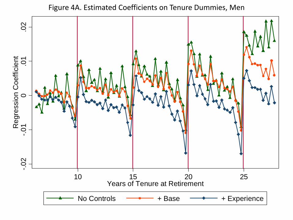
Figure 4 illustrates the coe¢ cients on the tenure dummies from the estimated regres-
sions. Following the institutional background, we estimate separate speci�cations for men
and women. Consistent with Figure 3, the coe¢ cients illustrate distinct decreases and
increases in the probability of retirement just before and after the thresholds respectively.
The plots also illustrates that the pattern in the estimated coe¢ cients does not change
signi�cantly when including a large set of base control variables. The base controls include
dummies for the following variables: calendar year, age measured in years, blue collar job
8
designation, two-digit industry classi�cations, nine geographic regions, quarter-of-year, �rm
size, health status at age 54, health in the current quarter, earnings growth over the past
quarter, and earnings growth over the same quarter in the past year.6 In addition, the base
controls include 10 piece splines in total real earnings through age 54 and total real earnings
in the current quarter. The plots in Figure 4 also show that, after including controls for
experiences (dummies for insurance and contribution years), the retirement-tenure gradi-
ent in the coe¢ cients becomes much �atter. This change highlights two features. First,
individuals with higher years of tenure generally have higher years of experience. Second,
after controlling for experience and other observables, there is little correlation between
tenure and retirement. Comparing the plots for men and women, women appear much
more responsive to the severance payments than men.
3.1.3 Gender Di¤erences
To investigate the di¤erences between men and women further, we return to the cross-
sectional variation based on observations at retirement and re-weight the observations for
men to be similar to those of women based on observables (see DiNardo, Fortin and Lemieux
(1996)). We implement the reweighting in the following steps. First we pool the observa-
tions for men and women and estimate a probit, Pr(femalei = 1jxi) = Pr(xi� + "i > 0).The observables xi include the values at retirement for the base and experience controls in
the regressions above. Next, we obtain the �tted probabilities for men and created weighted
counts using these �tted probabilities. Figure 5 plots the distributions of tenure at retire-
ment for men, women and the reweighted men. These plots indicate that di¤erences in
the observables do not account for the observed di¤erences between men and women. In
particular, while men and women do have di¤erences in observables such as retirement
age, earnings, health, experience, industries, and �rm size, accounting for the di¤erences in
these and other observables does not account for the di¤erential responsiveness to the sev-
erance payments. We discuss potential uses for the severance payments and corresponding
unobserved di¤erences that could explain this gender di¤erential in more detail below.
6Firm size is grouped into the following categories: � 5, 6�10; 11�25; 26�99; 100�499; 500�999;� 1000.Health status through age 54 is based on the following categories of sick leave through age 54: � 0:5 years,0:5� 1 years, 1� 2 years, and � 2 years. Health in the current quarter is based on the following categoriesfor sick leave in the current quarter: 0 days, 1 � 30 days, 31 � 60 days, and � 61 days. Earnings growthdummies are based on positive, negative, or zero growth relative to earnings in the corresponding quarter.Quarterly earnings for individuals with continuous employment during a calendar year are equal to totalannual earnings divided by 4. Earnings for individuals retiring at the beginning of a quarter are set equalto earnings from the previous quarter. For women, the base controls also include a dummy for having kids.
9

3.1.4 Job Starts
While the earlier �gures highlight individuals�responsiveness to the severance payments
at retirement, we now turn to investigating whether or not these payments a¤ect individuals
decisions to begin new jobs. Speci�cally, we investigate whether or not individuals time
the beginning of new jobs so that they can retire at the Early Retirement Ages (ERAs,
respectively 55 and 60 for women and men) and also claim severance payments at the time
of their retirements. To explore this idea, Figure 6 plots the number of individuals starting
new jobs (vertical axis) against age measured at a quarterly frequency (horizontal axis). In
individuals are timing the beginning of their new jobs so that they can just complete 10, 15,
or 20 years of tenure at the ERAs, then we would expect to see sharp increases in the number
of individuals starting new jobs at ages 50, 45, 40 etc. The evidence in Figure 5 shows no
discernible change in job starts at any age prior to the ERAs. This smoothness across age
emphasizes that, while there is evidence that some individuals delay their retirements to
qualify for (larger) severance payments at retirement, there is no evidence that individuals
reallocate their labor supply (or participation) are earlier ages in response to the sizeable
anticipated incentives from the severance payments.
3.1.5 Survey Responses
The full sample evidence aggregates over a variety of subsamples. To motivate and orga-
nize the analysis of heterogeneity across the subsamples, we present evidence on individuals�
reasons for retirement, employment situations and expectations regarding lump-sum pay-
ments at retirement. Table 2 presents survey responses regarding reasons for retirement
for men and women separately. For both groups, the most frequently cited reasons for
retirement are (1) becoming eligible for a public pension and (2) own ill health. For men,
employment circumstances (made redundant and being o¤ered early retirement options)
constitute the majority of the remaining reasons for retirement. For women, family cir-
cumstances (spending more time with the family and health of relatives) in addition to
the employment circumstances constitute the remaining reasons for retirement. Table 3
presents responses to questions regarding job security, job satisfaction and expectations
regarding lump sum payments at retirement. The responses indicate that most men and
women have job security, are satis�ed with their jobs and are aware of lump-sum payments
at retirement. In regard to awareness, roughly 47% and 42% of men and women expect to
receive lump-sum payments with their pension bene�ts, and these percentages are consis-
10

tent with the distribution of tenure at retirement which indicates that about 38% and 45%
of men and women respectively have more than 10 years of tenure at retirement.
These survey responses highlight they the types of individuals that are likely to be
responsive to the severance payments and also the circumstances that are likely to cause or
inhibit this responsiveness. Speci�cally, the responses motivate the following organization
for the heterogeneity analysis below. First, we examine heterogeneity related to public
pension eligibility and, more generally, the institutional framework of the pension system.
Second, we examine heterogeneity related to health. Third, we examine heterogeneity
related to wages and job separations.
3.2 Heterogeneity related to Public Pensions
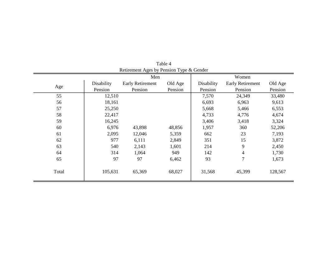
Following the institutional background of the Austrian pension system, we study het-
erogeneity related to public pensions by separating men and women and grouping the
retirement pensions into three categories: (1) disability pensions, which are based on re-
duced working capacity (2) early retirement pensions, which are based on eligibility prior
to the statutory retirement ages (60 and 65 for women and men respectively) and (3) old
age pensions. Table 4 presents retirement ages within each pension category. The table
indicates that, for men, a signi�cant amount of retirement occurs prior to age 60 through
disability pensions. For women, a signi�cant amount of retirement occurs between ages 55
through 60 through old age pensions.
Figure 7 presents the distributions of tenure at retirement within each gender and
pension type. Comparing the top �gures to the bottom �gures, the plots indicate that
women are uniformly more responsive to the severance payments than men. We discuss
the factors that could potentially account for this di¤erence between men and women
in greater detail below. Additionally, the plots indicate that men and women retiring
through disability pensions are relatively unresponsive to the severance payment incentives.
Intuitively, individuals who claim disability pensions may have poor health which inhibits
them from responding to the severance payment incentives. We examine heterogeneity
based on health in more detail below.
Plots of the distributions of tenure at retirement by gender and retirement age are
consistent with the plots by gender and pension type. Amongst men, there is little pooling
amongst those retiring prior to age 60, and individuals retiring at age 60 or beyond both
demonstrate similarly noticeable pooling. For women, there is noticeable pooling at all
11

retirement ages, though relatively more signi�cant pooling amongst those retiring beyond
age 60.
We next examine heterogeneity across individuals with di¤erent public pension bene�ts.
Bene�t levels are determined based on individuals�highest 15 years of earnings, and since
earnings are generally increasing in age, the highest earning years tend to be the years
prior to retirement. We therefore group individuals based on their gender and average real
earnings between ages 50 through 54 and compare the distributions of tenure at retirement
for the highest and lowest 15% within each gender. These distributions are presented in
Figure 8. The plots indicate more distinctive pooling patterns amongst men and women
with lower bene�t levels. Intuitively, the severance payments represent larger fractions of
wealth for these individuals with lower bene�ts and thus, these individuals face relatively
larger incentives to delay their retirements. Continuing with this intuition, individuals
with high earnings growth at older ages also face relatively larger incentives to delay their
retirements since the severance payments are larger fractions of their wealth. Plots of the
distributions of tenure at retirement for individuals with high and low earnings growth at
older ages indicate that there is indeed more pooling amongst men and women with high
earnings growth prior to retirement.
We investigate the di¤erences between men and women further by focusing �rst on
di¤erences based on experience and children. Because of the institutional setting, women
can retire at younger ages than men and will therefore have lower years of experience than
men. If di¤erences based on experience can account for the observed di¤erences between
men and women, then we expect women with high years of experience to have similar
patterns to those of men. Additionally, since the pension system counts maternity leave
toward years of experience when computing bene�ts, we also separate women with children
from those without children with the hypothesis that women without children and with
high experience are likely to be similar to men. Figure 9 presents the distributions of
tenure at retirement for women based on experience at age 55 and children. High and
low experience is based on the top and bottom quartiles of the experience distribution.
These plots indicate no sharp di¤erences based on experience, implying that experience
alone cannot account for the observed di¤erences between men and women. The plots
also indicate noticeably more pooling amongst women with children. The presence of
children may a¤ect the potential uses of the severance payments thereby making women
more responsive to the payments. We discuss potential uses of the severance payments and
di¤erence between men and women based on other observables in more detail below.
12

3.3 Heterogeneity related to Health
Wemeasure health at retirement using the number of days of sick leave an individual has
taken between age 54 and retirement. Roughly 35% of individuals have no sick leave over
their entire careers and 68% have no sick leave between ages 54 and retirement. Amongst
those with some sick leave between age 54 and retirement, we distinguish between those
in the top quartile of the sick leave distribution within each gender (high sick leave) from
those in the bottom three quartiles (low sick leave). This distinction is made to separate
those with extremely poor health status from others.
Figure 10 presents the distributions of tenure at retirement based on gender and health
at retirement. The plots indicate that there is no noticeable pooling amongst men and
women in extremely poor health. Thus, some of the pre-threshold retirement is likely to be
driven by negative health shocks and also more permanently poor health status. Amongst
those with low sick leave, there is less pooling amongst men than women; this could re�ect
that men on sick leave tend to be in worse health than women on sick leave.
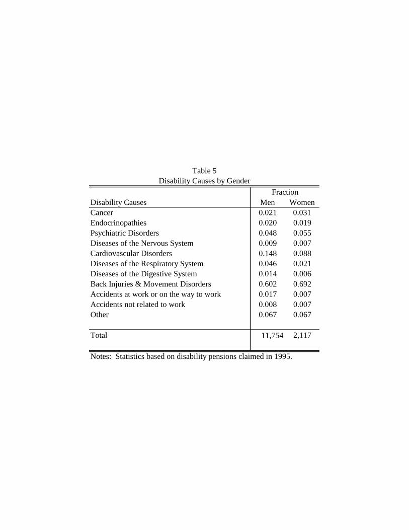
Consistent with the earlier evidence by pension type, roughly 64% of individuals with
some sick leave between age 54 and retirement claim disability pensions as opposed to
15% amongst those with no sick leave between age 54 and retirement. To provide some
context for the injuries causing sick leave and disability, Table 5 present the disability causes
amongst those claiming disability pensions in 1995. The statistics indicate that back injuries
and movement disorders are the most signi�cant causes of disabilities as these injuries
account for roughly 60% and 69% of disabilities amongst men and women respectively.
The second-most signi�cant cause of disabilities is cardiovascular disorders which account
for roughly 15% and 9% of injuries for men and women respectively. Amongst the remaining
disability causes, accidents at work and diseases of the respiratory system are more common
for men while psychiatric disorders are more common for women. Since the 2000 pension
reform, disability requirement have been increased so that there has been a reduction in
disability due to back injuries and movement disorders and also an increase in disability
due to mental illness.
We next examine industry-level di¤erences in health at retirement. Table 6 presents
statistics on the distribution of health at retirement across industries. Amongst men, poor
health at retirement is prevalent amongst those in construction and manufacturing and less
prevalent amongst those in the service industry. For women, those in sales and services
have better health at retirement. The services industry thus has relatively low rates of
disability for both men and women, but roughly 25% of men are in the services industry
13

while 48% of women are in the services industry.
Figures 11A&B present the distributions of tenure at retirement across aggregated
industries for men and women separately. The plots indicate less pooling amongst indi-
viduals in agriculture and mining, manufacturing and construction as compared to sales,
transportation and services. Intuitively, individuals in more physically demanding jobs may
have a high marginal disutility of work so that they are not likely to delay their retirements
to qualify for a (larger) severance payment. Indeed, for both men and women, the plots for
those within the services industry indicate more willingness to delay retirement, and these
jobs are less likely to be very physically demanding. Analysis using further disaggregated
industry classi�cations con�rms the pattern observed using the aggregate industry clas-
si�cations, namely that there is less pooling amongst individuals in industries with high
fractions of individuals with poor health at retirement. Examples of disaggregated indus-
try classi�cations with high fractions of individuals in poor health at retirement include
manufacturing of chemicals and chemical products (men) and manufacturing of textiles
(women). Examples of disaggregated industry classi�cations with high fractions of indi-
viduals in good health at retirement include �nancial intermediation (men) and real estate
activities (women).
3.4 Heterogeneity related to Job Separations
Involuntary separations may inhibit individuals from delaying their retirements to qual-
ify for (larger) severance payments. While it is not possible to directly distinguish between
voluntary and involuntary separations using the administrative data, we present evidence
in regard to involuntary separations in two ways. First, we examine the distributions of
tenure at retirement at di¤erent points in the business cycle. In particular, we group cal-
endar years based on having GDP growth rates above or below the average growth rate for
the sample period and then examine the distributions of tenure at retirement within these
above and below average growth categories. Intuitively, there may be less pooling amongst
those retiring during times of low economic growth because a larger portion of these retire-
ments may be involuntary during these times. Figure 12 presents this plot. While there
is still noticeable pooling during the lower growth periods, the plot indicates more distinct
pooling amongst men and women retiring during high growth periods. This evidence is
consistent with the intuition that individuals are more able to delay their retirements in
response to the severance payments during periods of strong macroeconomic growth.
14

We study pre-threshold retirement over the business cycle more explicitly in Figure 13.
In this �gure, we examine whether or not retirement before a tenure threshold varies over
the business cycle. We de�ne pre-threshold retirements as retirements occurring within one
year prior to a tenure threshold. Our hypothesis is that some pre-threshold retirements
may be involuntary so that, since overall involuntary retirements are countercyclical, the
fraction of retirements that are pre-threshold will be countercyclical as well. Figure 13
presents the time series plot of the fraction of pre-threshold retirements and the time series
for GDP growth. Consistent with the hypothesis, the fraction of retirements that are pre-
threshold does follow a mildly countercyclical patter. Thus, the evidence in Figures 10 and
11 suggests that some of the observed pre-threshold retirements are driven by the presence
of involuntary separations at retirement.
3.5 Discussion
The graphical analysis highlights excess retirements just after the tenure thresholds and
reduced retirements just before the thresholds. The analysis of heterogeneity illustrates
that interactions with public pension incentives, health status and job separations are
important factors a¤ecting individuals�responsiveness to the severance payment incentives.
Overall, the graphical evidence indicates a relatively low degree of observed intertemporal
substitution in retirement decisions. This conclusion follows from the observation that the
reduced frequency of retirements just prior to the tenure thresholds occurs within roughly
1 year prior to the threshold even though individuals face wage increases based on sizeable
fractions of their annual earnings.
We present evidence on individuals�uses of lump-sum gifts to gain some insights as to
why the willingness to delay retirement decisions is seemingly low. Table 7 presents survey
responses of older workers regarding their likely uses of an unanticipated lump-sum gift of
12,000 euros. While the question is in regard to an unanticipated gift, individuals uses of
an anticipated gift may be similar. The results in Table 7 indicate that about two thirds
of individuals would save some of the gift, and amongst the savers, about two thirds of
the gift would be saved. Few individuals report that they would use any of the gift to pay
o¤ debts, though the individuals that would use the gift to pay o¤ debts would use just
over half of the gift. Of the remaining uses, both men and women are highly likely to give
some of the gift to relatives or others and to use some of the gift to take a vacation. The
responses for women indicate that they are more likely to give some of the gift to relatives,
15

and conditional on giving, they would give larger gifts. In contrast, men report a higher
likelihood of using some of the gift to purchase durable goods. Given these responses, it
seems plausible that individuals may not be willing to delay their retirements by more than
a year to increase their savings and take a vacation when beginning retirement.
4 Elasticity Estimation
4.1 Model
Consider an intertemporal labor supply model in which an individual has quasi-linear
preferences over consumption in each period, ct, and years of work, R. We assume that
there is no time discounting and that the individual lives for T periods. We abstract from
uncertainty in the presentation of the model. However, in the presence of uncertainty (e.g.
wage uncertainty, mortality), the model can be interpreted as capturing decisions based on
certainty equivalences because of the assumption of risk neutrality following from the quasi-
linear preferences. At time 0, the individual decides how much to consume in each period
and how many years to work. Heterogeneity in labor supply across di¤erent individuals
results from heterogeneity in the taste for work, which is denoted by � and distributed in the
population according to the density function f(�). Formally, the individual�s optimization
problem is given by
maxfctg;R
TXt=0
ct ��
1 + 1e
�R
�
�1+ 1e
s.t.TXt=0
ct = wR + x
where w denotes the individual�s wage rate per year of tenure completed and x denotes
non-wage income.
The assumption of quasi-linear preferences is motivated by the graphical analysis.
Quasi-linear preferences imply that there are no income e¤ects in individuals�labor sup-
ply functions. This lack of income e¤ects is consistent with the graphical analysis which
presents evidence that income e¤ects are not detectable in the distribution of tenure at
retirement. Intuitively, the severance payments are small relative to lifetime income, and
individuals may be unlikely to respond to such small changes in lifetime income.
16

The elasticity of intertemporal substitution in labor supply is de�ned to capture how
labor supply responds to wage variation holding the marginal utility of income constant,d lnRd lnw
j� where � denotes the marginal utility of income. In this model, the marginal utilityof income is equal to 1, and from the individual�s labor supply function, we have
d lnR
d lnwj� = e:
This elasticity captures an individual�s responsiveness to an anticipated wage increase.
When a wage increase is anticipated, it is already factored into lifetime income so that the
marginal utility of income can be assumed to be held constant by construction. Intuitively,
when the marginal disutility from additional labor supply rises very rapidly, an individual
will not adjust his labor supply very much in response to an anticipated wage increase.
In this setting, the intertemporal (Frisch) labor supply elasticity coincides with the sta-
tic income-constant (Marshallian) and utility-constant (Hicksian) labor supply elasticities.
Though the are conceptually distinct, these labor supply elasticities coincide in this setting
because there are no income e¤ects by assumption (see Browning (2005)). Nonetheless, we
refer to e as an intertemporal elasticity because the variation that will be used to identify
and estimate this parameter will correspond to anticipated, within-person variation in wage
rates over time periods.
4.2 Pooling & a Semiparametric Elasticity Estimator
In this section we introduce a discontinuity in the budget constraint and discuss how
pooling at this discontinuity can be used to estimate the intertemporal elasticity. Optimal
retirement choices with this discontinuity are presented graphically in Figure 14. Speci�-
cally, suppose that at a threshold level of tenure at retirement �R, individuals qualify for a
lump-sum payment denoted by dx.
First, we characterize the types of individuals who locate at the threshold in the presence
of the discontinuity. Let [�,��] denote the set of types that choose labor supply �R. The
highest skill level the locates at �R is the highest skill level that located at �R even in the
absence of the discontinuity; that is, �� is characterized by �� such that �R = ��we. Next, the
lowest skill level that locates at �R is the skill level that is indi¤erent between choosing �R
and his counterfactual labor supply in the scenario without the discontinuity. Therefore, �
17

is characterized � that satis�es the following indi¤erence condition
w(�we) + x� �
1+ 1e
( �we
�)1+
1e = w �R + x+ dx� �
1+ 1e
(�R�)1+
1e
where the left-hand side captures counterfactual utility without the discontinuity and op-
timal retirement equal to �we and the right-hand side captures utility when locating at the
threshold and receiving the lump-sum payment.
Second, we relate the set of types that pool at the threshold labor supply level to
changes in wages and labor supply. Let R denote the counterfactual labor supply of type
�, R = �we. Thus, dR = �R�R captures the change in labor supply for this individual dueto the discontinuity. For a type-� individual, the change in labor supply can be related to a
wage change. In particular, the wage that would have lead type � to choose labor supply �R
in the absence of the discontinuity is given by ~w such that �R = � ~we. In computing ~w, the
variation from the income discontinuity dx is converted into wage variation. Using these
characterizations of wages and labor supply, the proportional change in labor supply due
to the discontinuity is given by
dR�R=�R�R�R
= 1��w~w
�eThese changes in optimal retirement are depicted in Figure 15.
Next, we write the amount of pooling at the threshold labor supply in terms of the
changes in labor supply and the counterfactual distribution of labor supply without the
discontinuity. Let P denote the fraction of the population pooling (i.e. the excess mass)
at the threshold labor supply level, and let h0(R) denote the density of the population
choosing labor supply R when there is no discontinuity in the budget constraint. This
density results from the labor supply function and the density of tastes for work; that is,
the labor supply function R = �we implies that h0(R) = 1wef( R
we) where f(:) denotes the
density of tastes for work. Given the de�nitions and characterizations above, individuals
with tastes � 2 [�; ��] pool at the threshold and these individuals have counterfactual labor
18

supply choices R 2 [R; �R]. The amount of pooling is then given by
P =
Z �R
R
h0(R)@R
� dR
�h0(R) + h0( �R)
2
�= �R
h1�
�w~w
�ei�h0(R) + h0( �R)2
�where the second line follows from a trapezoidal approximation of the integral and the last
line uses the above characterization of the change in labor supply.
This last equation yields an estimator for the intertemporal elasticity based on the
amount of pooling around the threshold labor supply level. In particular, this equation
can be solved to express the intertemporal elasticity in terms of observable parameters and
estimable variables,
e = e(w; dx; �R| {z }observable
; h0(R); h0( �R); P| {z }estimable
):
The wage, threshold and lump-sum payment are all assumed to be observable. The density
at the cuto¤ and the threshold and the amount of pooling can be estimated using the
empirical distribution of tenure completed by retirement.
4.3 Elasticity Estimator with Frictions
We introduce frictions into the model above to account for the observed, pre-threshold
retirement patterns. The graphical evidence in Figure 3 illustrates positive numbers of
individuals retiring just prior to the thresholds and also that the number of individuals
retiring just before the thresholds decreases as the time until the threshold decreases.
We model frictions as adjustment costs in retirement decisions. let R0 denote an indi-
vidual�s (counterfactual) retirement choice in the absence of the severance payment and let
R1 denote the same individual�s retirement choice in the presence of the severance payment.
We denote the utility gain from adjusting from R0 to R1 by �U . Given an adjustment cost
�, the individual will adjust his retirement choice only if the gain exceeds the cost, i.e. if
and only it � < �U . We assume that adjustment costs are randomly distributed on [0; �H ]
where �H > 0 with density and distribution functions �(:) and �(:) respectively.
The frictions a¤ect the estimation of the structural parameter e since only individuals
19

with su¢ ciently low costs can pool at the threshold. In particular, the amount of pooling
at the threshold is given by
P =
Z �R
R
Z �U(R)
0
�(�)h0(R)@�@R
=
Z �R
R
�(�U(R))h0(R)dR
This change in the excess mass at the tenure thresholds due to the frictions is illustrated in
Figure 16. Using a similar trapezoidal approximation and also a similar derivation of dR as
in case without frictions, the amount of pooling at the tenure threshold can be re-written
as
P � dR
��h0(R) + ��h0( �R)
2
�= �R
h1�
�w~w
�ei��h0(R) + ��h0( �R)2
�where � = �(�U(R)) denotes the probability of switching for individuals who are just
indi¤erent between their choices with and without the discontinuities and �� = �(�U( �R))
denotes the probability of switching for individuals locating exactly at the threshold. Notice
that by the indi¤erence condition, �U(R) = 0 and hence � = 0. The above equation can
be solved to yield an estimator for the structural parameter e,
e = e(w; dx; �R; ��| {z }observed
; h0( �R); P| {z }estimated
):
Compared to the case without frictions, the estimator with frictions introduces one addi-
tional observable, ��, which re�ects that only a fraction of individuals near the threshold
have su¢ ciently low costs to switch retirement choices. When allowing for these frictions,
the responsiveness to wage variation will not be captured by the structural parameter e
only. Intuitively, when there is wage variation, individuals will only respond to the wage
variation if they have su¢ ciently low costs, so the intertemporal elasticity of substitution
in labor supply is given by E = �(�U)e, i.e. the structural parameter must be adjusted
by the probability of switching.
20

4.4 Estimating Pooling & the Counterfactual Density
The estimation of the counterfactual density and the amount of pooling at the threshold
can be seen as follows. We start with the observed frequencies of individuals retiring at each
level of tenure Rt; we denote these frequencies by fh(Rt)gt=1:::T : We estimate regressionsof the form
h(Rt) = ~h(Rt) + ~"t
where the function ~h(R) denotes a high-order (8th order) continuous polynomial function in
tenure at retirement. We estimate separate regressions between each of the tenure thresh-
olds to fully capture the observed discontinuous patterns at each threshold. Using the
estimated polynomial function, we predict frequencies to obtain a continuous polynomial
approximation for the observed frequencies.7 Figure 17 illustrates this polynomial approx-
imation against the observed frequencies. We adopt the frequencies from the polynomial
approximation as the "actual" frequencies. By using the polynomial approximation, we
are able to adjust for spikes at the integer values of tenure at retirement.
Next, we use these actual frequencies to obtain counterfactual frequencies. These coun-
terfactual frequencies aim to capture what the frequencies would have looked like in the
absence of the severance payment incentives. We assume that in the absence of the sev-
erance payments, individuals retiring at the tenure thresholds would behave similarly to
individuals between or away from the tenure thresholds. With this identifying assumption
in mind, we estimate the counterfactual density by regressing the observed density on a
continuous (8th order) polynomial function and a set of dummies capturing behavior near
the threshold,~h(Rt) = h0(Rt) +
X�R=10;15;20;25
Xj
1(Rj near �R) + "t:
As illustrated in Figure 18, the estimated polynomial function h0(R) re�ects what the labor
supply choices would have been in the absence of the severance payments. To obtain the
�nal estimated counterfactual frequencies, we re-scale the �tted values fh0(Rt)gt=1:::T sothat the total number of predicted retirements across all tenure levels obtained using only
the polynomial function equals the total number of observed retirements. This re-scaling
is motivated by the reasoning that the total number of retirements would not change in
the counterfactual and moreover, any changes in the total number of predicted retirements
7We re-scale the predicted frequencies so that the total number of predicted retirements equal the totalnumber of observed retirements.
21

are assumed to spread across the tenure levels in proportion to the predicted number of
retirements at each tenure level.
While there is no pre-determined method to determine which levels of labor supply
are �near� the threshold, we will rely on a graphical method as illustrated in Figure 19.
In particular, the graphical evidence suggests that responses to the discontinuities are
generally within �1 year of each tenure threshold. We also rely on a graphical methodto estimate the amount of pooling at the threshold labor supply level. While the model
above predicts that individuals will choose to locate exactly at the threshold level of labor
supply �R, it is plausible that individuals will delay their retirement to qualify for the bonus
lump-sum payment and then retire shortly after the threshold. For this reason, we select
a high cuto¤ level of labor supply R based on the graphical evidence such that there is
no graphical evidence for excess mass beyond this high cuto¤. The amount of pooling or
excess mass near the threshold is then captured by integrating the observed density net
of the estimated counterfactual between the threshold and this high cuto¤. The graphical
evidence indicates that the excess mass beyond each tenure threshold is generally within 1
year after each threshold, so we select R = �R + 1.
To summarize, the estimators for each of the estimable terms are
h0(R) : h0(R) = g(R) where R is selected graphically
h0( �R) : h0( �R) = g( �R) where �R is known by assumption
P : P =R R�R[h(R)� g(R)]@R where R is selected graphically.
4.5 Estimation Details
Given the observed and estimated terms, the estimator is implemented at each threshold
using the following iterative algorithm. First, we start with an arbitrary positive elasticity,
e0. Second, we compute � using the given elasticity and the indi¤erence condition. Third,
we solve for ~w using � and the given elasticity e0. Fourth, we compute a new elasticity e1using the pooling equation and ~w. We then set e1 = e0 and iterate until there is convergence
between e1 and e0.
4.6 Estimation Results
Before turning to the elasticity estimates, we focus �rst on the estimation results for
the amount of excess mass at each tenure threshold. These results are presented in Table
8. The �rst column presents the estimated excess mass at each tenure thresholds where
22

excess mass is capturing the corresponding shaded area illustrated in Figure 19. To put the
magnitude of this area in better perspective, the second column of Table 8 presents this area
as a fraction of the total amount of mass prior to each threshold between R and �R. Overall,
the excess mass is a relatively low fraction of the total mass even though wage incentives are
sizeable. Column 3 of Table 8 presents an alternative measure of excess mass based on the
pre-threshold reduced mass illustrated in Figure 19. Theoretically, this measure of excess
mass should be equal to that presented in the �rst column of Table 8 since the amount of
individuals delaying their retirements should be equal to the amount of excess individuals
pooling at or just beyond the thresholds. We formally (statistically) test for equality
in these two excess mass measures in column 4 of Table 8 which presents the di¤erence
between these two measures and the corresponding standard errors of the di¤erence. With
the exception of the last threshold, it does not appear that there any statistically signi�cant
di¤erences between the two measures. Thus, the estimation procedure appears consistent
with the model presented above.
Table 9 presents the baseline intertemporal elasticity estimates at each tenure thresh-
old using the full sample of retirements. The estimates in the �rst column are based on
assuming that the discontinuity in the budget constraint dx is the same fraction of lifetime
income at each threshold (0:5%). These estimates indicate very low intertemporal elastic-
ities on the order of roughly 0:02. The small magnitude of these elasticities is driven by
the relatively low excess mass measures and the high wage incentives. The estimates in
the third column are based on an alternative calibration of dx in which the discontinuities
are decreasing fractions of lifetime income at each threshold (0:5%, 0:367%, 0:233%, and
0:100% respectively). The smaller discontinuities imply lower wage incentives than those
used to estimate the elasticities in the �rst column. As a result of the lower wage incentives,
the elasticities in the second column are larger than the estimates in the �rst column.
The remaining columns present estimates when allowing for frictions. Column 3 of
Table 9 presents estimates of �� which measures the fraction of counterfactual pre-threshold
individuals that have su¢ ciently low frictions so that they can delay their retirements to
just beyond the thresholds. These estimates highlight that relatively few individuals are
predicted to have su¢ ciently low frictions.
Intuitively, the relatively few individuals with su¢ ciently low frictions will be predicted
to be relatively responsive to account for the observed excess mass. Thus the estimated
intertemporal elasticities with the frictions will be larger than those estimates in columns 1
and 2. Columns 4 and 5 present the estimated intertemporal elasticities when accounting
23

for the frictions. Using discontinuities based on a constant fraction of lifetime income at
each threshold, the estimates in column 4 are between roughly 0:02 and 0:18, about one
order of magnitude larger than the elasticities without frictions. Assuming that the discon-
tinuities dx are declining fractions of lifetime income, the estimates in column 5 are between
0:10 and 0:18. Thus, even when accounting for the frictions, the estimated intertemporal
elasticities are small compared to estimates and calibrated values from previous studies
because, at each threshold, the wage incentives from the severance payments are relatively
large compared to the excess mass.
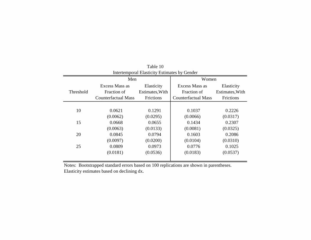
Table 10 presents separate elasticity estimates for men and women. The estimates
elasticities in this table are all based on the model with frictions and the speci�cation with
dx declining across each threshold. Consistent with the graphical evidence, the estimated
elasticities for men are lower than the corresponding estimates for women at each threshold.
In particular, estimated elasticities for men range from 0:07 to 0:13 while the estimated
elasticities for women range from 0:10 to 0:23.
Overall, the intertemporal elasticity estimates are relatively low in magnitude when
compared to estimates and calibrated values from previous studies (for examples, see Mul-
ligan (1999) and King and Rebelo (1999)). These low elasticity estimates result from the
combination of relatively small excess mass and relatively large wage incentives at each
tenure threshold.
5 Conclusion
This paper presents evidence on individuals�willingness to delay exiting the labor force
in response to anticipated changes in wage rates. This evidence is based on discontinu-
ous increases in retirement bene�ts upon completion of 10, 15, 20, and 25 years of tenure
by retirement. The graphical evidence indicates that most individuals do not delay their
retirements by more than 1 year in response to 33% or larger increases in their annual
wage rates. An analysis of heterogeneity indicates that poor health and business cycle
�uctuations leading to involuntary job separations reduce intertemporal substitution. Ad-
ditionally, women demonstrate more willingness to delay their retirements in response to
the anticipated �nancial gains at the tenure thresholds. Estimated elasticities con�rm the
results of the graphical analysis. These results based on the extensive margin of labor
supply suggest that intertemporal substitution in labor force participation may not be as
high as suggested by some previous macroeconomic studies.
24

References
Altonji, J. G. (1986). Intertemporal substitution in labor supply: Evidence from micro
data. Journal of Political Economy 94 (3), S176�S215.
Blundell, R. and T. Macurdy (1999). Labor supply: A review of alternative approaches.
In O. Ashenfelter and D. Card (Eds.), Handbook of Labor Economics, Volume 3 of
Handbook of Labor Economics, Chapter 27, pp. 1559�1695. Elsevier.
Blundell, R., C. Meghir, and P. Neves (1993). Labour supply and intertemporal substi-
tution. Journal of Econometrics 59 (1-2), 137�160.
Brown, K. (2009). The Link between Pensions and Retirement Timing: Lessons from
California Teachers. Working paper, University of Illinois at Urbana-Champaign.
Browning, M. (2005). A working paper from april 1985: Which demand elasticities
do we know and which do we need to know for policy analysis? Research in Eco-
nomics 59 (4), 293�320.
Card, D., R. Chetty, and A. Weber (2007). Cash-on-Hand and Competing Models of
Intertemporal Behavior: New Evidence from the Labor Market. Quarterly Journal
of Economics 122 (4), 1511�1560.
Chetty, R. (2009). Bounds on elasticities with optimization frictions: A synthesis of
micro and macro evidence on labor supply. Working Paper 15616, National Bureau
of Economic Research.
Chetty, R., J. N. Friedman, T. Olsen, and L. Pistaferri (2009). Adjustment costs, �rm
responses, and labor supply elasticities: Evidence from danish tax records. Working
Paper 15617, National Bureau of Economic Research.
DiNardo, J., N. Fortin, and T. Lemieux (1996). Labor market institutions and the dis-
tribution of wages, 1973-1992: A semiparametric approach. Econometrica 64 (5),
1001�1044.
Heckman, J. J. (1993). What has been learned about labor supply in the past twenty
years? American Economic Review 83 (2), 116�121.
King, R. G. and S. T. Rebelo (1999). Resuscitating real business cycles. In J. B. Taylor
and M. Woodford (Eds.), Handbook of Macroeconomics, Volume 1, Chapter 14, pp.
927�1007. Elsevier.
25
Krueger, A. and J. Pischke (1992). The E¤ect of Social Security on Labor Supply: A
Cohort Analysis of the Notch Generation. Journal of Labor Economics 10 (4), 412�
437.
Looney, A. and M. Singhal (2006). The e¤ect of anticipated tax changes on intertemporal
labor supply and the realization of taxable income. Working Paper 12417, National
Bureau of Economic Research.
MaCurdy, T. E. (1981). An empirical model of labor supply in a life-cycle setting. Journal
of Political Economy 89 (6), 1059�85.
Manoli, D., K. Mullen, and M. Wagner (2010). Pension Bene�ts and Retirement Deci-
sions: Income vs. Price Elasticities. Working paper, University of California - Los
Angeles.
Mulligan, C. B. (1999). Substition over time: Another look at life-cycle labor supply.
In B. Bernanke and J. Rotemberg (Eds.), NBER Macroeconomics Annual 1998, Vol-
ume 13, pp. 75�152. MIT Press.
Rogerson, R. and J. Wallenius (2009). Micro and macro elasticities in a life cycle model
with taxes. Journal of Economic Theory 144 (6), 2277�2292.
Saez, E. (1999). Do taxpayers bunch at kink points? Working Paper 7366, National
Bureau of Economic Research.
Saez, E. (2010). Do taxpayers bunch at kink points? American Economic Journal:
Economic Policy (forthcoming).
Ziliak, J. P. and T. J. Kniesner (1999). Estimating life cycle labor supply tax e¤ects.
Journal of Political Economy 107 (2), 326�359.
Zweimüller, J., R. Winter-Ebmer, R. Lalive, A. Kuhn, J.-P. Wuellrich, O. Ruf, and
S. Büchi (2009). Austrian social security database. NRN: The Austrian Center for
Labor Economics and the Analysis of the Welfare State (Working Paper 0903).
26

Full Sample Tenure at Retirement ≥ 10 Full Sample Tenure at Retirement ≥ 10
# of Individuals 239,027 90,668 205,534 91,481
Age 59.61 60.00 58.06 58.1460.00 60.00 57.75 57.752.21 2.21 2.64 2.81
Tenure 8.79 16.92 9.70 15.997.08 15.67 8.67 15.177.56 5.41 6.77 4.58
Severance Pay 5535.67 14593.61 2928.24 6578.990.00 11809.12 0.00 4806.29
9314.31 9824.80 5822.16 7220.87
Annual Earnings 23208.73 26808.22 11601.37 13007.3322656.78 26587.60 9971.90 11523.0611383.31 10797.06 10376.58 11285.80
Lifetime Earnings 794832.00 851188.40 455786.40 490604.80782837.30 835394.40 416443.50 449005.50281017.60 254134.50 231449.40 223546.80
Lifetime Employment Time 34.24 37.81 24.81 28.9337.77 40.36 26.50 29.8910.69 8.00 10.60 7.89
Lifetime Sick Leave 0.62 0.50 0.40 0.350.28 0.17 0.08 0.060.93 0.83 0.80 0.73
Fractions:Claiming Disability Pensions 0.442 0.352 0.154 0.110Claiming Early Retirement Pensions 0.273 0.371 0.221 0.296Claiming Old Age Pensions 0.285 0.276 0.626 0.594
Agriculture & Mining 0.065 0.066 0.029 0.021Manufacturing 0.274 0.293 0.189 0.165Construction 0.195 0.089 0.030 0.029Sales 0.161 0.161 0.185 0.156Tourism 0.021 0.012 0.064 0.031Transportation 0.054 0.054 0.024 0.027Services 0.231 0.325 0.479 0.571
Table 1Summary Statistics
Notes: Except for the Fractions, the mean, median and standard deviations are reported for each variable. All earnings variables are expressed in 2008 euros. Summary statistics for lifetime earnings are based on birth cohorts beyond 1935. Employment Time and Sick Leave are measured in years.
Men Women

Men Women 1. Became eligible for public pension 65.84 65.41 2. Became eligible for private occupational pension 2.12 0.87 3. Became eligible for a private pension 1.06 0.15 4. Was offered an early retirement option/window (with special incentives or bonus) 5.31 2.62 5. Made redundant (for example pre-retirement) 5.84 4.80 6. Own ill health 23.54 16.72 7. Ill health of relative or friend 0.18 2.47 8. To retire at same time as spouse or partner 0.35 1.89 9. To spend more time with family 0.88 7.27 10. To enjoy life 2.30 1.74
# of Respondents 565 688
Table 2Reasons for Retirement
Notes: Data from Waves 1 & 2 of SHARE Austria. The percentages do not sum to 100 since respondents could select all reasons that apply.
% Yes

Men Women
1. % Strongly Agree 5.56 3.852. % Agree 17.68 12.093. % Disagree 47.47 40.664. % Strongly Disagree 29.29 43.41
# of Respondents 198 183
Men Women1. % Strongly Agree 45.45 48.632. % Agree 48.48 44.813. % Disagree 5.56 6.564. % Strongly Disagree 0.51 0# of Respondents 198 183
Men Women% Yes 46.91 41.67# of Respondents 194 168
B. All things considered, I am satisfied with my job.
C. Expecting to receive lump sum payment with pension entitlement?
Notes: Data from Waves 1 & 2 of SHARE Austria. The number of respondents is reported in brackets.
Table 3Employment Responses
A. My job security is poor.
Age Disability Pension
Early Retirement Pension
Old Age Pension
Disability Pension
Early Retirement Pension
Old Age Pension
55 12,510 7,570 24,349 33,48056 18,161 6,693 6,963 9,61357 25,250 5,668 5,466 6,55358 22,417 4,733 4,776 4,67459 16,245 3,406 3,418 3,32460 6,976 43,898 48,856 1,957 360 52,20661 2,095 12,046 5,359 662 23 7,19362 977 6,111 2,849 351 15 3,87263 540 2,143 1,601 214 9 2,45064 314 1,064 949 142 4 1,73065 97 97 6,462 93 7 1,673
Total 105,631 65,369 68,027 31,568 45,399 128,567
Table 4Retirement Ages by Pension Type & Gender
Men Women
Disability Causes Men WomenCancer 0.021 0.031Endocrinopathies 0.020 0.019Psychiatric Disorders 0.048 0.055Diseases of the Nervous System 0.009 0.007Cardiovascular Disorders 0.148 0.088Diseases of the Respiratory System 0.046 0.021Diseases of the Digestive System 0.014 0.006Back Injuries & Movement Disorders 0.602 0.692Accidents at work or on the way to work 0.017 0.007Accidents not related to work 0.008 0.007Other 0.067 0.067
Total 11,754 2,117
Disability Causes by Gender
Notes: Statistics based on disability pensions claimed in 1995.
Fraction
Table 5

Industry N Any Sick Leave
Mean Sick Leave
Median Lifetime
Sick Leave
Claiming Disability N Any Sick
LeaveMean Sick
Leave
Median Lifetime
Sick Leave
Claiming Disability
Agriculture & Mining 28,486 0.356 0.124 0.258 0.405 8,156 0.206 0.069 0.079 0.212Manufacturing 119,548 0.463 0.174 0.351 0.467 62,205 0.274 0.101 0.167 0.159Construction 55,651 0.550 0.207 0.504 0.568 8,124 0.162 0.061 0.000 0.114Sales 53,562 0.330 0.136 0.121 0.368 52,191 0.177 0.071 0.000 0.117Tourism 5,778 0.435 0.186 0.266 0.476 14,853 0.329 0.112 0.167 0.264Transportation 19,540 0.472 0.202 0.364 0.444 7,586 0.379 0.224 0.237 0.169Services 92,180 0.222 0.087 0.082 0.286 142,688 0.190 0.068 0.033 0.124
Table 6Health at Retirement by Gender & Industry
Women
Notes: These statistics include observations with left-censored tenure at retierment. Sick Leave measures the number of days on sick leave between ages 54 and retirement. Lifetime sick leave measures the number of sick days through retirement. Claiming Disability measures the fraction of individuals claiming disability pensions.
Men

% Using Any Average AmountAverage Amount Conditional on
Using Any% Using Any Average Amount
Average Amount Conditional on
Using Any 1. Save or invest 0.69 5910.82 8593.933 0.66 5329.31 8115.472
(0.46) (4871.54) (3379.12) (0.48) (4829.60) (3590.46) 2. Pay off debts 0.10 740.34 7257.58 0.07 475.40 6634.33
(0.30) (2495.16) (3721.29) (0.26) (1993.01) (3838.19) 3. Give to relatives or donation 0.45 2940.34 6470.75 0.57 4074.97 7161.84
(0.49) (4167.61) (3920.77) (0.50) (4626.04) (3936.06) 4. Buy durables 0.23 1137.56 4939.60 0.19 853.64 4483.99
(0.42) (2664.34) (3475.26) (0.40) (2264.29) (3268.65) 5. Holiday or journey 0.30 1270.94 4174.11 0.29 1266.68 4370.30
(0.46) (2681.27) (3393.39) (0.45) (2637.03) (3231.34)
Table 7Uses of Unexpected Gift of 12,000 Euros
Notes: Data from Waves 1 & 2 of SHARE Austria. Standard deviations are shown in parentheses.
Men (N=647) Women (N=935)

Threshold Excess Mass (P)
Excess Mass as Fraction of
Counterfactual Pre-Threshold Mass
Reduced MassExcess Mass
Minus Reduced Mass
10 282.4181 0.0837 257.7642 24.6540(14.1547) (0.0045) (27.8781) (35.5396)
15 243.5809 0.1064 252.2882 -8.7073(11.2730) (0.0054) (21.3307) (26.7132)
20 180.9516 0.1238 222.8940 -41.9424(10.1030) (0.0077) (16.4108) (23.6186)
25 61.9577 0.0792 120.0253 -58.0676(8.6186) (0.0122) (15.7863) (22.0346)
Table 8Excess Mass Estimates
Notes: Bootstrapped standard errors based on 100 replications are shown in parentheses.

Threshold Constant dx Declining dx Friction, Constant dx Declining dx
10 0.0316 0.0316 0.3630 0.1779 0.1779(0.0032) (0.0032) (0.0188) (0.0238) (0.0238)
15 0.0231 0.0300 0.4645 0.1062 0.1430(0.0021) (0.0028) (0.0205) (0.0119) (0.0161)
20 0.0181 0.0345 0.5473 0.0690 0.1429(0.0020) (0.0041) (0.0220) (0.0096) (0.0203)
25 0.0056 0.0206 0.5648 0.0217 0.0987(0.0030) (0.0060) (0.0354) (0.0073) (0.0350)
Table 9Intertemporal Elasticity Estimates, Full Sample
Notes: Bootstrapped standard errors based on 100 replications are shown in parentheses.
Elasticity Estimates, No Frictions Elasticity Estimates,With Frictions
Π
ThresholdExcess Mass as
Fraction of Counterfactual Mass
Elasticity Estimates,With
Frictions
Excess Mass as Fraction of
Counterfactual Mass
Elasticity Estimates,With
Frictions
10 0.0621 0.1291 0.1037 0.2226(0.0062) (0.0295) (0.0066) (0.0317)
15 0.0668 0.0655 0.1434 0.2307(0.0063) (0.0133) (0.0081) (0.0325)
20 0.0845 0.0794 0.1603 0.2086(0.0097) (0.0200) (0.0104) (0.0310)
25 0.0809 0.0973 0.0776 0.1025(0.0181) (0.0536) (0.0183) (0.0537)
Table 10
Notes: Bootstrapped standard errors based on 100 replications are shown in parentheses. Elasticity estimates based on declining dx.
Men WomenIntertemporal Elasticity Estimates by Gender

0.3
33.5
.75
1Fr
actio
n of
Las
t Yea
r's S
alar
y
0 5 10 15 20 25 30Years of Tenure
Payment Amounts based on Tenure at Retirement
Figure 1

0.2
.4.6
.81
Sur
vivo
r Fun
ctio
n
55 56 57 58 59 60 61 62 63 64 65 66 67 68 69 70Age
Men Women
Figure 2. Survivor Functions for Men and Women

010
0020
0030
0040
00In
divi
dual
s
10 15 20 25Years of Tenure at Retirement
Figure 3: Distribution of Tenure at Retirement, Monthly Frequency
-.02
-.01
0.0
1.0
2R
egre
ssio
n C
oeffi
cien
t
10 15 20 25Years of Tenure at Retirement
No Controls + Base + Experience
Figure 4A. Estimated Coefficients on Tenure Dummies, Men

-.05
0.0
5.1
Reg
ress
ion
Coe
ffici
ent
10 15 20 25Years of Tenure at Retirement
No Controls + Base + Experience
Figure 4B. Estimated Coefficients on Tenure Dummies, Women

050
010
0015
0020
00In
divi
dual
s
5 10 15 20 25 30Years of Tenure at Retirement
Women Men Reweighted Men
Figure 5: Distribution of Tenure at Retirement by Gender

020
0040
0060
0080
00#
of In
divi
dual
s S
tarti
ng N
ew J
obs
40 41 42 43 44 45 46 47 48 49 50 51 52 53 54 55 56 57 58 59 60Age
All Women Men
Figure 6: Number of New Job Starts by Age

050
010
0015
00
200
400
600
800
050
010
0015
00
020
040
060
0
050
010
00
010
0020
0030
0010 15 20 25 10 15 20 25 10 15 20 25
Men, Disability Men, Early Retirement Men, Old Age
Women, Disability Women, Early Retirement Women, Old Age
Indi
vidu
als
Years of Tenure at Retirement
Figure 7. Distribution of Tenure at Retirement by Gender & Retirement Pension Type

020
040
060
00
200
400
600
10 15 20 25 10 15 20 25
Men - Low AvgEarn Men - High AvgEarn
Women - Low AvgEarn Women - High AvgEarn
Indi
vidu
als
Years of Tenure at Retirement
Figure 8. Distribution of Tenure at Retirement by Gender & Pension Benefits

050
010
0015
00
050
010
0015
00
010
020
030
0
050
010
00
10 15 20 25 10 15 20 25
Low Expr, No Children Low Expr, Children
High Expr, No Children High Expr, Children
Indi
vidu
als
Years of Tenure at Retirement
Figure 9. Distribution of Tenure at Retirement for Women by Experience at Age 55 & Child Status
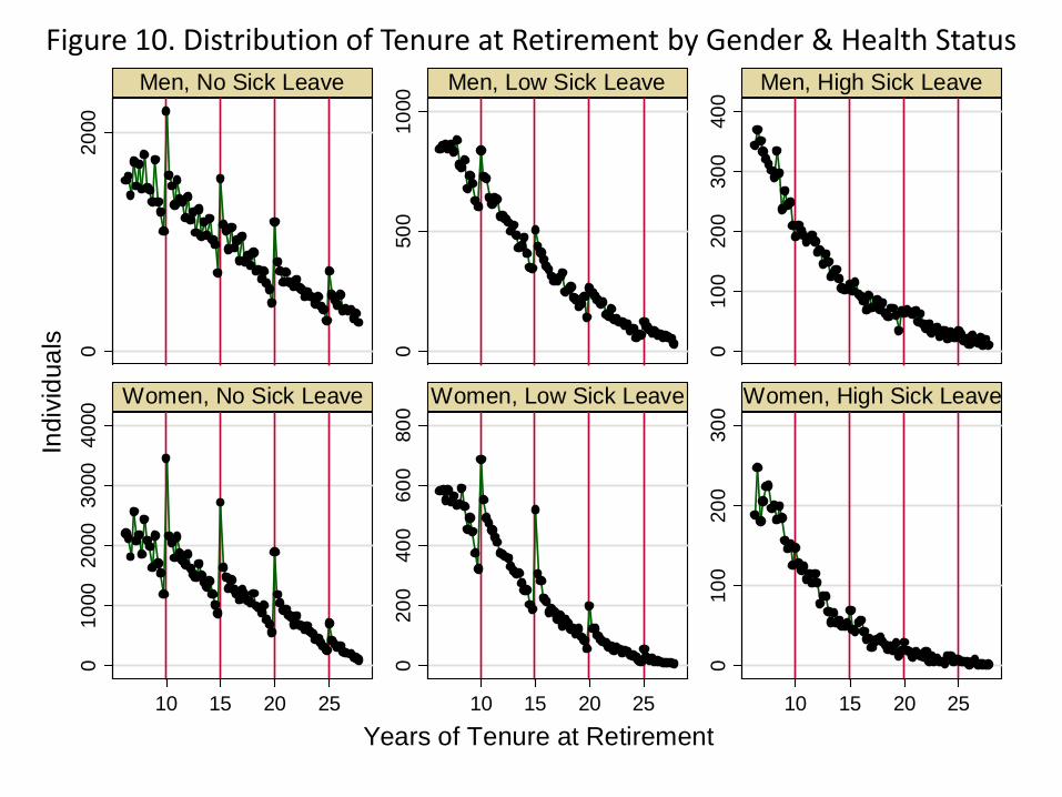
020
00
050
010
00
010
020
030
040
0
010
0020
0030
0040
00
020
040
060
080
0
010
020
030
010 15 20 25 10 15 20 25 10 15 20 25
Men, No Sick Leave Men, Low Sick Leave Men, High Sick Leave
Women, No Sick Leave Women, Low Sick Leave Women, High Sick Leave
Indi
vidu
als
Years of Tenure at Retirement
Figure 10. Distribution of Tenure at Retirement by Gender & Health Status

050
100
150
200
050
010
00
010
020
030
040
0
020
040
060
0
050
100
150
050
010
0010 15 20 25 10 15 20 25 10 15 20 25
Agriculture & Mining Manufacturing Construction
Sales Transportation Services
Indi
vidu
als
Years of Tenure at Retirement
Figure 11A. Distribution of Tenure at Retirement by Industry, Men
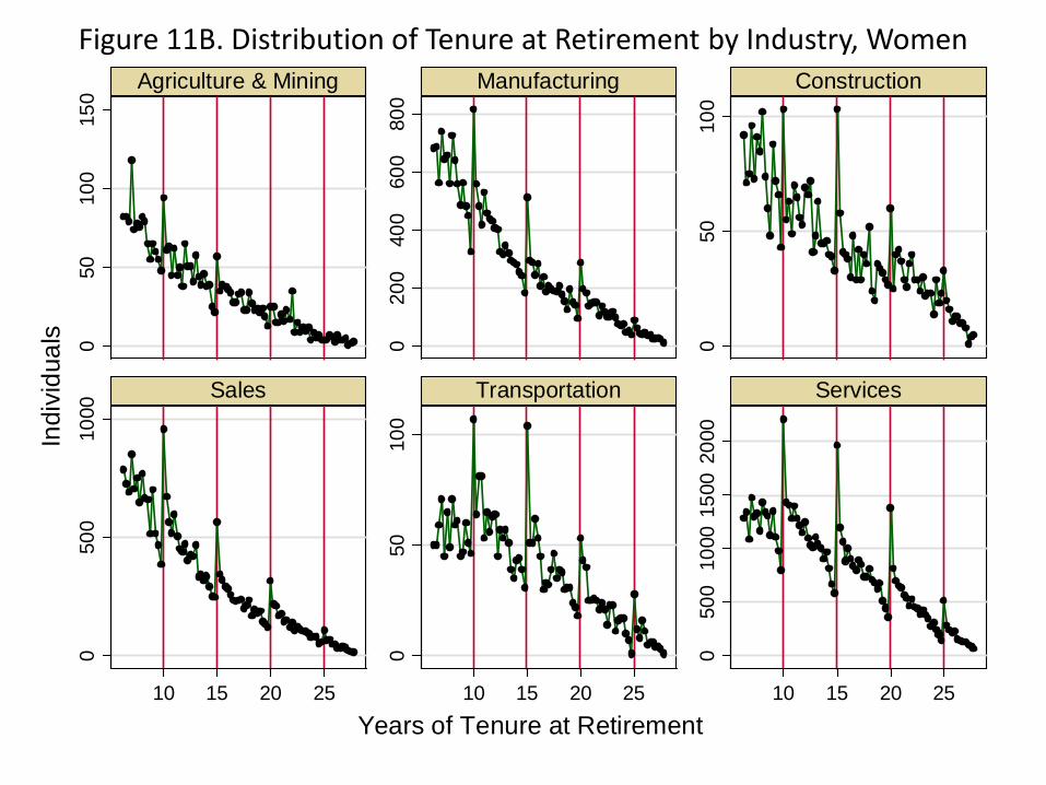
050
100
150
020
040
060
080
0
050
100
050
010
00
050
100
050
010
0015
0020
0010 15 20 25 10 15 20 25 10 15 20 25
Agriculture & Mining Manufacturing Construction
Sales Transportation Services
Indi
vidu
als
Years of Tenure at Retirement
Figure 11B. Distribution of Tenure at Retirement by Industry, Women

050
010
0015
00
050
010
0015
0020
00
050
010
0015
0020
00
010
0020
0030
00
10 15 20 25 10 15 20 25
Men, Below Avg Men, Above Avg
Women, Below Avg Women, Above Avg
Indi
vidu
als
Years of Tenure at Retirement
Figure 12. Distribution of Tenure at Retirement by Gender & GDP Growth

0.0
1.0
2.0
3.0
4G
DP
Gro
wth
Rat
e
.04
.06
.08
.1.1
2Fr
actio
n of
Sam
ple
Ret
irem
ents
dur
ing
Yea
r
1985 1987 1989 1991 1993 1995 1997 1999 2001 2003 2005Calendar Year
Pre-Threshold Retirement GDP Growth Rate
Figure 13. Probabilities of Pre-Threshold Retirement over the Business Cycle

Labor Supply
$
RR
Type θ’s indifference curve
dx
Type θ’s indifference curve
Figure 14. Optimal Retirement Choices with Discontinuity

Labor Supply
$
RR
Slope = w
Type θ’s indifference curve
dx
Figure 15. Changes in Optimal Retirement
dR
~
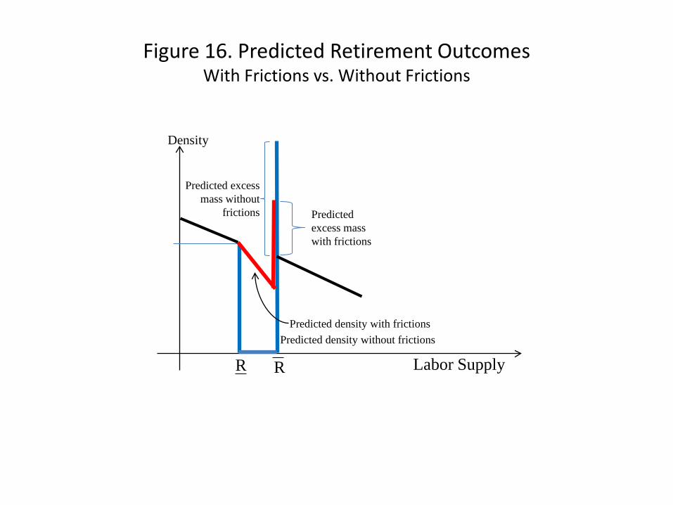
Labor Supply
Density
R R
Predicted density without frictionsPredicted density with frictions
Predicted excess mass without
frictions Predicted excess mass with frictions
Figure 16. Predicted Retirement OutcomesWith Frictions vs. Without Frictions

010
0020
0030
0040
00In
divi
dual
s
10 15 20 25Years of Tenure at Retirement
Observed Approximation
Polynomial Approximation of FrequenciesFigure 17

050
010
0015
0020
0025
00In
divi
dual
s
10 15 20 25Years of Tenure at Retirement
Counterfactual Actual
Counterfactual FrequenciesFigure 18

Individuals, h0(R)
Years of Tenure at Retirement
Counterfactual Actual
Estimation of Critical Values
Figure 19
R R R
Excess massReduced mass