Linear Least Squares

• Suppose we are given a set of data points {(xi, fi)}, i = 1, . . . , n. Thesecould be measurements from an experiment or obtained simply by evaluatinga function at some points. One approach to approximating this data is tointerpolate these points, i.e., find a function (such as a polynomial of degree≤ (n − 1) or a rational function or a piecewise polynomial) which passesthrough all n points.

• However, it might be the case that we know that these data points shouldlie on, for example, a line or a parabola, but due to experimental error theydo not. So what we would like to do is find a line (or some other higherdegree polynomial) which best represents the data. Of course, we need tomake precise what we mean by a “best fit” of the data.

• As a concrete example suppose we have n points

(x1, f1), (x2, f2), · · · (xn, fn)

which we expect to lie on a straight line but due to experimental error, theydon’t.

•We would like to draw a line and have the line be the best representation ofthe points in some sense. If n = 2 then the line will pass through both pointsand so the error is zero at each point. However, if we have more than twodata points, then we can’t find a line that passes through the three points(unless they happen to be collinear) so we have to find a line which is a goodapproximation in some sense.

• An obvious approach would be to create an error vector ~e of length n whereeach component measures the difference

ei = fi − y(xi) where y = a1x + a0 is line fitting data.

Then we can take a norm of this error vector and our goal would be to findthe line which minimizes the norm of the error vector.

• Of course this problem is not clearly defined because we have not specifiedwhat norm to use.

• The linear least squares problem finds the line which minimizes this error vectorin the ℓ2 (Euclidean) norm.

• In some disciplines this is also called linear regression.

Example We want to fit a line p1(x) = a0 + a1x to the data points

(1, 2.2), (.8, 2.4), (0, 4.25)

in a linear least squares sense. For now, we will just write the overdeterminedsystem and determine if it has a solution. We will find the line after we investigatehow to solve the linear least squares problem. Our equations are

a0 + a1 · 1 = 2.2a0 + a1 · .8 = 2.4a0 + a1 · 0 = 4.25 (1)

Writing this as a matrix problem A~x = ~b we have1 11 0.81 0

(a0a1

)=

2.22.44.25

Now we know that this over-determined problem has a solution if the right handside is in R(A) (i.e., it is a linear combination of the columns of the coefficientmatrix A). Here the rank of A is clearly 2 and thus not all of IR3. Moreover,(2.2, 2.4, 4.25)T is not in the R(A), i.e., not in the span{(1, 1, 1)T , (1, 0.8, 0)T}and so the system doesn’t have a solution. This just means that we can’t find aline that passes through all three points.

If our data had been

(1, 2.1) (0.8, 2.5) (0, 4.1)

then we would have had a solution to the over-determined system. Our matrix

problem A~x = ~b is 1 11 0.81 0

(a0a1

)=

2.12.54.1

and we notice that in this case, the right hand side is in R(A) because2.12.54.1

= 4.1

111

− 2

10.80

and thus the system is solvable and we have the line 4.1 − 2x which passesthrough all three points.

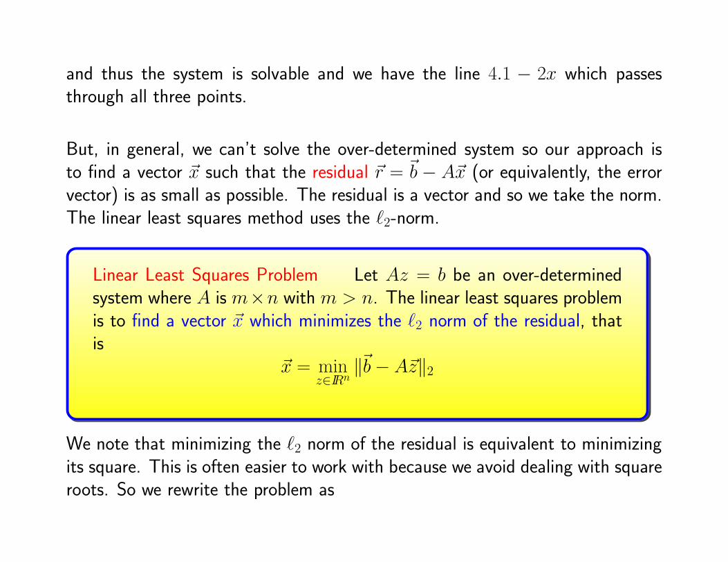
But, in general, we can’t solve the over-determined system so our approach isto find a vector ~x such that the residual ~r = ~b − A~x (or equivalently, the errorvector) is as small as possible. The residual is a vector and so we take the norm.The linear least squares method uses the ℓ2-norm.

Linear Least Squares Problem Let Az = b be an over-determinedsystem where A is m×n with m > n. The linear least squares problemis to find a vector ~x which minimizes the ℓ2 norm of the residual, thatis

~x = minz∈IRn

‖~b− A~z‖2

We note that minimizing the ℓ2 norm of the residual is equivalent to minimizingits square. This is often easier to work with because we avoid dealing with squareroots. So we rewrite the problem as

Find a vector ~x which minimizes the square of the ℓ2 norm

~x = min~z∈IRn

‖~b− A~z‖22

Example For our example where we want to fit a line p1(x) = a0 + a1x to thedata points

(1, 2.2), (.8, 2.4), (0, 4.25)

we can calculate the residual vector and then use techniques from Calculus tominimize ‖~r‖2

2.

~r =

2.22.44.25

−

1 11 0.81 0

(z1z2

)=

2.2− z1 − z22.4− z1 − 0.8z2

4.25− z1

To minimize ‖~r‖22we take the first partials with respect to z1 and z2 and set

them equal to zero. We have

f = ‖~r‖22= (2.2− z1 − z2)

2 + (2.4− z1 − .8z2)2 + (4.25− z1)

2

and thus∂f

∂z1= −4.4+2z1+2z2− 4.8+2z1+1.6z2− 8.5+2z1 = 17.7+6z1+3.6z2 = 0

∂f

∂z2= −4.4 + 2z1 + 2z2 − 3.84 + 1.6z1 + 1.28z2 = −8.24 + 3.6z1 + 3.28z2 = 0

So we have to solve the linear system(

6 3.63.6 3.28

)(z1z2

)=

(−17.78.24

)

whose solution is (4.225,−2.125)T .

We now want to determine

1. Does the linear least squares problem always have a solution?

2. Does the linear least squares problem always have a unique solution?

3. How can we efficiently solve the linear least squares problem?

Theorem The linear least squares problem always has a solution. Itis unique if A has linearly independent columns. The solution of theproblem can be found by solving the normal equations

ATA~y = AT~b .

Before we prove this, recall that the matrix ATA is symmetric because

(ATA)T = AT (AT )T = ATA

and is positive semi-definite because

~xT (ATA)~x = (~xTAT )(A~x) = (A~x)T (A~x) = ~yT~y ≥ 0 where ~y = A~x

Now yTy is just the square of the Euclidean length of ~y so it is only zero if~y = ~0. Can ~y ever be zero? Remember that y = A~x so if ~x ∈ N (A) then~y = ~0. When can the rectangular matrix A have something in the null spaceother than the zero vector? If we can take a linear combination of the columns ofA (with coefficients nonzero) and get zero, i.e., if the columns of A are linearlydependent. Another way to say this is that if the columns of A are linearlyindependent, then ATA is positive definite; otherwise it is positive semi-definite

(meaning that xTATAx ≥ 0). Notice in our theorem we have that the solutionis unique if A has linearly independent columns. Another equivalent statementwould be to require N (A) = 0.

Proof First we show that the problem always has a solution. Recall that R(A)and N (AT ) are orthogonal complements in IRm. This tells us that we can writeany vector in IRm as the sum of a vector in R(A) and one in N (AT ). To this

end we write ~b = ~b1 +~b2 where ~b1 ∈ R(A) and ~b2 ∈ R(A)⊥ = N (AT ). Nowwe have the residual is given by

~b− A~x = (~b1 +~b2)− A~x

Now ~b1 ∈ R(A) and so the equation A~x = ~b1 is always solvable which says theresidual is

~r = ~b2

When we take the ‖~r‖2 we see that it is ‖~b2‖2; we can never get rid of this term

unless ~b ∈ R(A) entirely. The problem is always solvable and is the vector ~x

such that A~x = ~b1 where ~b1 ∈ R(A).

When does A~x = ~b1 have a unique solution? It is unique when the columns of

A are linearly independent or equivalently N (A) = ~0.

Lastly we must show that the way to find the solution ~x is by solving the normalequations; note that the normal equations are a square n× n system and whenA has linearly independent columns the coefficient matrix ATA is invertible withrank n. If we knew what ~b1 was, then we could simply solve A~x = ~b1 but wedon’t know what the decomposition of ~b = ~b1+~b2 is, simply that it is guaranteedto exist. To demonstrate that the ~x which minimizes ‖~b − A~x‖2 is found by

solving ATA~x = AT~b we first note that these normal equations can be writtenas AT (~b − A~x) = ~0 which is just AT times the residual vector so we need toshow AT~r = 0 to prove the result. From what we have already done we knowthat

AT (~b− A~x) = AT (~b1 +~b2 − A~x) = AT (~b2)

Recall that ~b2 ∈ R(A)⊥ = N (AT ) which means that AT~b2 = ~0 and we havethat

AT (~b− A~x) = ~0 =⇒ ATA~x = AT~b

The proof relies upon the fact that R(A) and N (AT ) are orthogonal comple-ments and that this implies we can write any vector as the sum of a vector in

R(A) and its orthogonal complement.

Example We return to our previous example and now determine the line whichfits the data in the linear least squares sense; after we obtain the line we willcompute the ℓ2 norm of the residual.

We now know that the linear least squares problem has a solution and in our caseit is unique because A has linearly independent columns. All we have to do isform the normal equations and solve as usual. The normal equations

(1 1 11 0.8 0

)1 11 0.81 0

(a0a1

)=

(1 1 11 0.8 0

)

2.22.44.25

are simplified as (3.0 1.81.8 1.64

)(a0a1

)=

(8.854.12

)

which has the solution (4.225,−2.125) giving the line y(x) = 4.225− 2.125x. If

we calculate the residual vector we have

2.2− y(1)2.4− y(0.8)4.25− y(0)

=

0.1−0.1250.025

which has an ℓ2 norm of 0.162019.

We said that we only talk about the inverse of a square matrix. However, onecan define a pseudo-inverse (or generalized inverse or Moore-Penrose inverse) ofa rectangular matrix. If A is an m×n matrix with linearly independent columnsthen a pseudo-inverse (or sometimes called left inverse ofA ) isA† = (ATA)−1AT

which is the matrix in our solution to the normal equations

~x = (ATA)−1AT~b

It is called the pseudo-inverse of the rectangular matrix A because[(ATA)−1AT

]A = (ATA)−1(ATA) = I

Note that if A is square and invertible the pseudo-inverse reduces to A−1 because

(ATA)−1AT = A−1(AT )−1AT = A−1 .

We can also find a polynomial of higher degree which fits a set of data. Thefollowing example illustrates this.

Example State the linear least squares problem to find the quadratic polynomialwhich fits the following data in a linear least squares sense; determine if it has aunique solution; calculate the solution and calculate the ℓ2 norm of the residualvector.

(0, 0) (1, 1) (3, 2) (4, 5)

In this case we seek a polynomial of the form p(x) = a0+ a1x+ a2x2. Our over

determined system is

1 0 01 1 11 3 91 4 16

a0a1a2

=

0125

So the linear least squares problem is to find a vector ~x in R3 which minimizes∥∥∥∥∥∥∥∥

0125

− A

z1z2z3

∥∥∥∥∥∥∥∥

2

2

for all ~z ∈ R3 where A is the 4 × 3 matrix given above. We see that A has

linearly independent columns so its rank is 3 and thus the linear least squaresproblem has a unique solution. The normal equations are

1 1 1 10 1 3 40 1 9 16

1 0 01 1 11 3 91 4 16

a0a1a2

=

1 1 1 10 1 3 40 1 9 16

0125

leading to the square system

4 8 268 26 9226 92 338

a0a1a2

=

82799

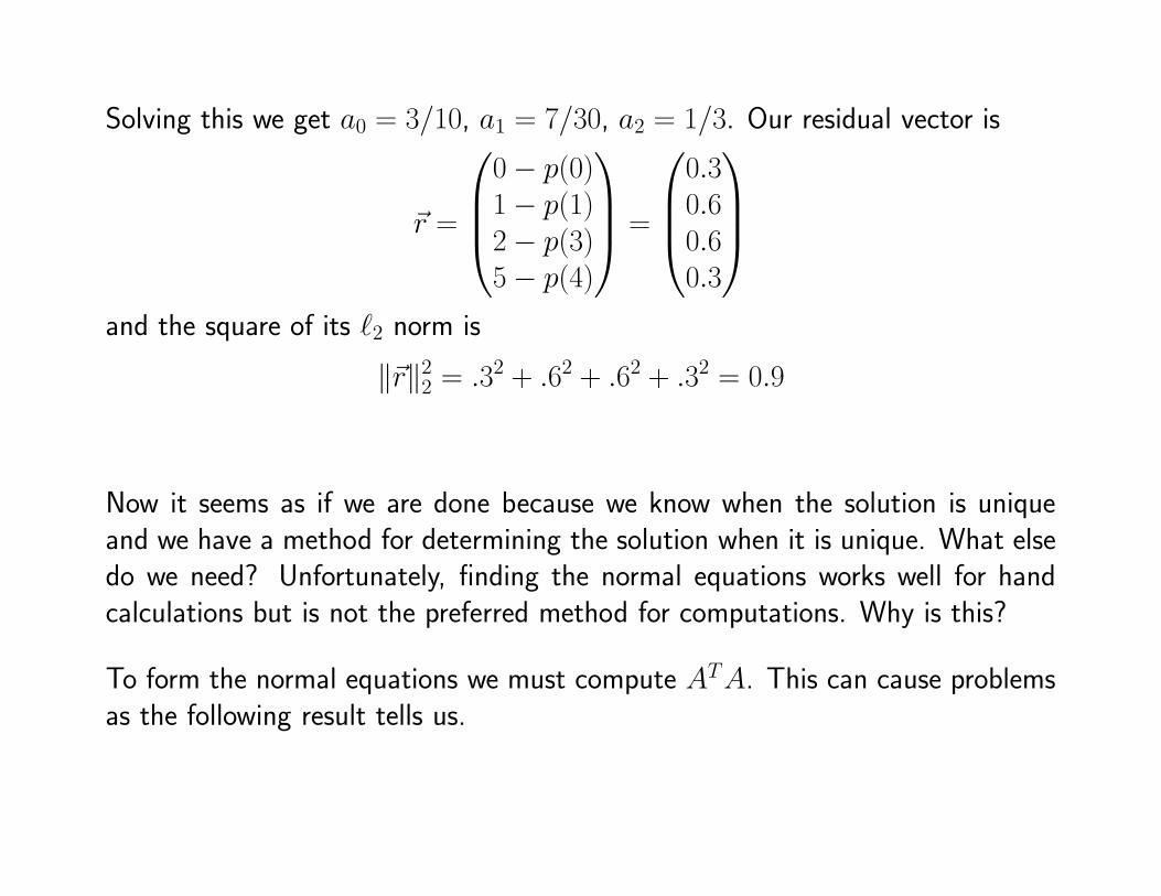
Solving this we get a0 = 3/10, a1 = 7/30, a2 = 1/3. Our residual vector is

~r =

0− p(0)1− p(1)2− p(3)5− p(4)

=

0.30.60.60.3

and the square of its ℓ2 norm is

‖~r‖22= .32 + .62 + .62 + .32 = 0.9

Now it seems as if we are done because we know when the solution is uniqueand we have a method for determining the solution when it is unique. What elsedo we need? Unfortunately, finding the normal equations works well for handcalculations but is not the preferred method for computations. Why is this?

To form the normal equations we must compute ATA. This can cause problemsas the following result tells us.

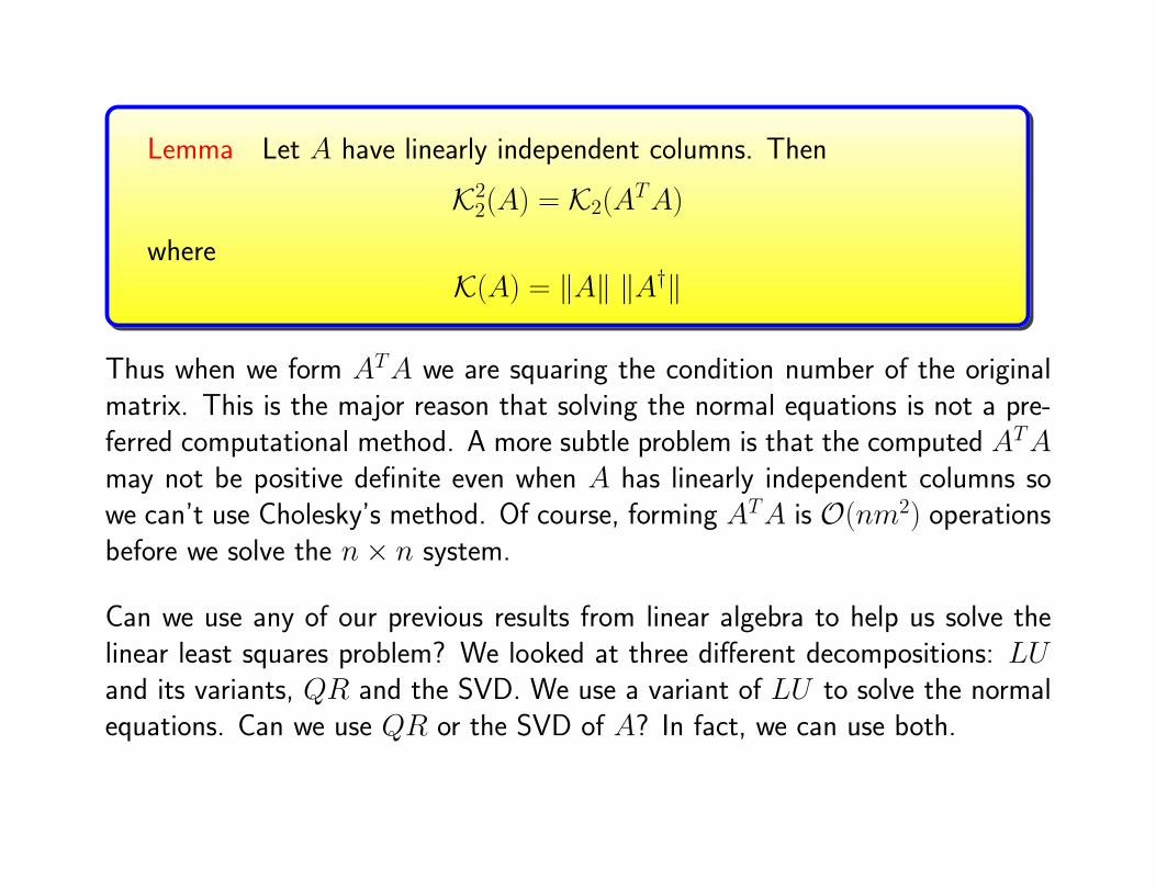
Lemma Let A have linearly independent columns. Then

K2

2(A) = K2(A

TA)

whereK(A) = ‖A‖ ‖A†‖

Thus when we form ATA we are squaring the condition number of the originalmatrix. This is the major reason that solving the normal equations is not a pre-ferred computational method. A more subtle problem is that the computed ATAmay not be positive definite even when A has linearly independent columns sowe can’t use Cholesky’s method. Of course, forming ATA is O(nm2) operationsbefore we solve the n× n system.

Can we use any of our previous results from linear algebra to help us solve thelinear least squares problem? We looked at three different decompositions: LUand its variants, QR and the SVD. We use a variant of LU to solve the normalequations. Can we use QR or the SVD of A? In fact, we can use both.

Recall that an m×n matrix with m > n and rank n has the QR decomposition

A = QR = Q

(R1

0

)

where Q is anm×m orthogonal matrix, R is anm×n upper trapezoidal matrix,R1 is an n × n upper triangular matrix and 0 represents an (m − n) × n zeromatrix.

Now to see how we can use the QR decomposition to solve the linear leastsquares problem, we take QT~r where ~r = ~b− A~x to get

QT~r = QT~b−QTA~x = QT~b−QTQ

(R1

0

)~x .

Now Q is orthogonal so QTQ = I so if we let QT~b = (~c, ~d)T , we have

QT~r = QT~b−

(R1

0

)~x =

(~c~d

)−

(R1~x0

)=

(c−R1~x

d

)

Now also recall that an orthogonal matrix preserves the ℓ2 length of any vector,i.e., ‖Q~y‖2 = ‖~y‖2 for Q orthogonal. Thus we have

‖QT~r‖2 = ‖~r‖2

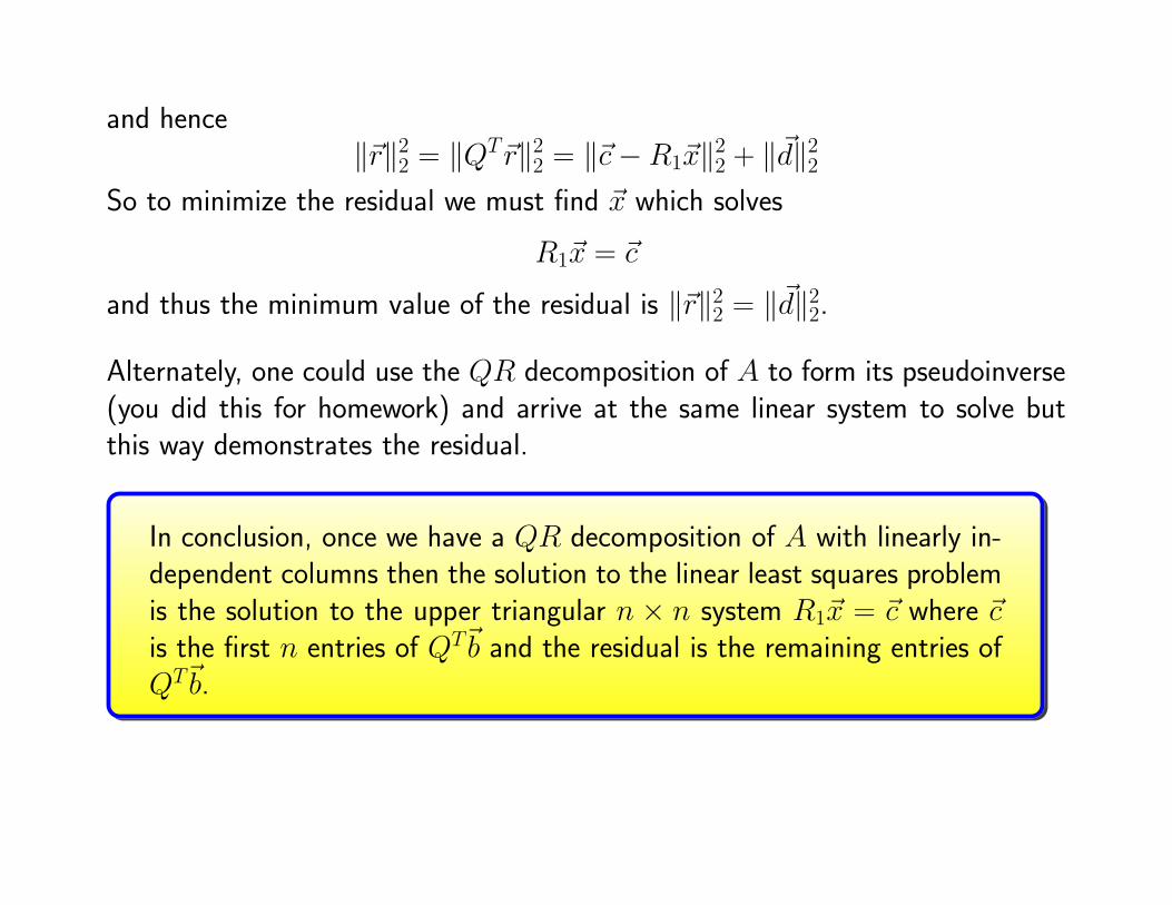
and hence‖~r‖2

2= ‖QT~r‖2

2= ‖~c−R1~x‖

2

2+ ‖~d‖2

2

So to minimize the residual we must find ~x which solves

R1~x = ~c

and thus the minimum value of the residual is ‖~r‖22= ‖~d‖2

2.

Alternately, one could use the QR decomposition of A to form its pseudoinverse(you did this for homework) and arrive at the same linear system to solve butthis way demonstrates the residual.

In conclusion, once we have a QR decomposition of A with linearly in-dependent columns then the solution to the linear least squares problemis the solution to the upper triangular n × n system R1~x = ~c where ~cis the first n entries of QT~b and the residual is the remaining entries ofQT~b.

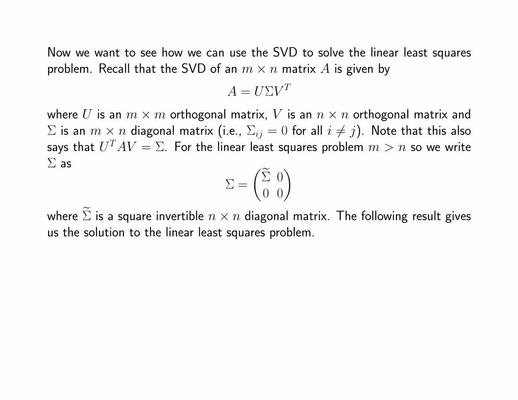
Now we want to see how we can use the SVD to solve the linear least squaresproblem. Recall that the SVD of an m× n matrix A is given by

A = UΣV T

where U is an m×m orthogonal matrix, V is an n× n orthogonal matrix andΣ is an m × n diagonal matrix (i.e., Σij = 0 for all i 6= j). Note that this alsosays that UTAV = Σ. For the linear least squares problem m > n so we writeΣ as

Σ =

(Σ̃ 00 0

)

where Σ̃ is a square invertible n× n diagonal matrix. The following result givesus the solution to the linear least squares problem.

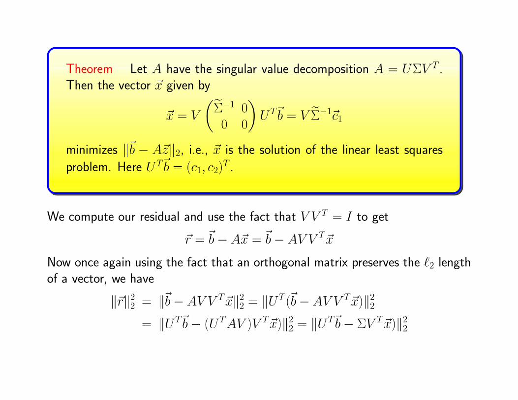
Theorem Let A have the singular value decomposition A = UΣV T .Then the vector ~x given by

~x = V

(Σ̃−1 00 0

)UT~b = V Σ̃−1~c1

minimizes ‖~b − A~z‖2, i.e., ~x is the solution of the linear least squares

problem. Here UT~b = (c1, c2)T .

We compute our residual and use the fact that V V T = I to get

~r = ~b− A~x = ~b− AV V T~x

Now once again using the fact that an orthogonal matrix preserves the ℓ2 lengthof a vector, we have

‖~r‖22= ‖~b− AV V T~x‖2

2= ‖UT (~b− AV V T~x)‖2

2

= ‖UT~b− (UTAV )V T~x)‖22= ‖UT~b− ΣV T~x)‖2

2

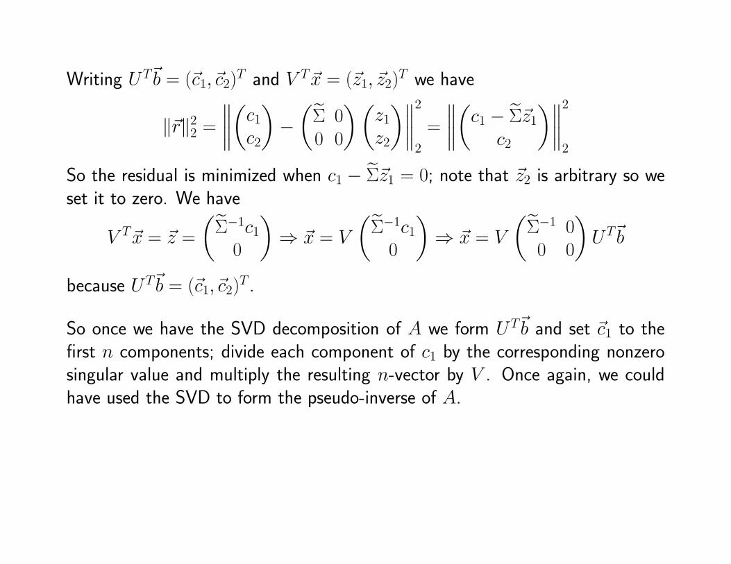
Writing UT~b = (~c1,~c2)T and V T~x = (~z1, ~z2)

T we have

‖~r‖22=

∥∥∥∥(c1c2

)−

(Σ̃ 00 0

)(z1z2

)∥∥∥∥2

2

=

∥∥∥∥(c1 − Σ̃~z1

c2

)∥∥∥∥2

2

So the residual is minimized when c1 − Σ̃~z1 = 0; note that ~z2 is arbitrary so weset it to zero. We have

V T~x = ~z =

(Σ̃−1c10

)⇒ ~x = V

(Σ̃−1c10

)⇒ ~x = V

(Σ̃−1 00 0

)UT~b

because UT~b = (~c1,~c2)T .

So once we have the SVD decomposition of A we form UT~b and set ~c1 to thefirst n components; divide each component of c1 by the corresponding nonzerosingular value and multiply the resulting n-vector by V . Once again, we couldhave used the SVD to form the pseudo-inverse of A.