Embed Size (px)
Citation preview
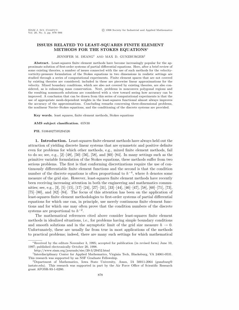
ISSUES RELATED TO LEAST-SQUARES FINITE ELEMENTMETHODS FOR THE STOKES EQUATIONS∗
JENNIFER M. DEANG† AND MAX D. GUNZBURGER‡
SIAM J. SCI. COMPUT. c© 1998 Society for Industrial and Applied MathematicsVol. 20, No. 3, pp. 878–906
Abstract. Least-squares finite element methods have become increasingly popular for the ap-proximate solution of first-order systems of partial differential equations. Here, after a brief review ofsome existing theories, a number of issues connected with the use of such methods for the velocity-vorticity-pressure formulation of the Stokes equations in two dimensions in realistic settings arestudied through a series of computational experiments. Finite element spaces that are not coveredby existing theories are considered; included in these are piecewise linear approximations for thevelocity. Mixed boundary conditions, which are also not covered by existing theories, are also con-sidered, as is enhancing mass conservation. Next, problems in nonconvex polygonal regions andthe resulting nonsmooth solutions are considered with a view toward seeing how accuracy can beimproved. A conclusion that can be drawn from this series of computational experiments is that theuse of appropriate mesh-dependent weights in the least-squares functional almost always improvesthe accuracy of the approximations. Concluding remarks concerning three-dimensional problems,the nonlinear Navier–Stokes equations, and the conditioning of the discrete systems are provided.
Key words. least squares, finite element methods, Stokes equations
AMS subject classification. 65N30
PII. S1064827595294526
1. Introduction. Least-squares finite element methods have always held out theattraction of yielding discrete linear systems that are symmetric and positive definiteeven for problems for which other methods, e.g., mixed finite element methods, failto do so; see, e.g., [2]–[48], [50]–[56], [58], and [60]–[84]. In many settings such as theprimitive variable formulation of the Stokes equations, these methods suffer from twoserious problems. The first is that conforming discretizations require the use of con-tinuously differentiable finite element functions and the second is that the conditionnumber of the discrete equations is often proportional to h−4, where h denotes somemeasure of the grid size. However, least-squares finite element methods have recentlybeen receiving increasing attention in both the engineering and mathematics commu-nities; see, e.g., [3], [5]–[15], [17]–[24], [27]–[31], [33]–[44], [46]–[47], [58], [60]–[71], [73],[75]–[80], and [82]–[84]. The focus of this attention has been on the application ofleast-squares finite element methodologies to first-order systems of partial differentialequations for which one can, in principle, use merely continuous finite element func-tions and for which one may often prove that the condition numbers of the discretesystems are proportional to h−2.
The mathematical references cited above consider least-squares finite elementmethods in idealized situations, i.e., for problems having simple boundary conditionsand smooth solutions and in the asymptotic limit of the grid size measure h → 0.Unfortunately, these are usually far from true in most applications of the methodsto practical problems; indeed, there are many such settings for which mathematical
∗Received by the editors November 3, 1995; accepted for publication (in revised form) June 10,1997; published electronically October 20, 1998.
http://www.siam.org/journals/sisc/20-3/29452.html†Interdisciplinary Center for Applied Mathematics, Virginia Tech, Blacksburg, VA 24061-0531.
This research was supported by an NSF Graduate Fellowship.‡Department of Mathematics, Iowa State University, Ames, IA 50011-2064 (gunzburg@
iastate.edu). This research was supported in part by the Air Force Office of Scientific Researchgrant AFOSR-93-1-0280.
878

LEAST-SQUARES METHODS FOR THE STOKES EQUATIONS 879
theories have not yet been developed. Often, complex combinations of boundaryconditions are needed and solutions are not smooth enough to recover the full accuracyof the finite element functions used. Moreover, often the grid sizes used are notsufficiently small to be in the asymptotic range of mathematical error estimates. Insuch cases, a naive implementation of least-squares finite element methods may lead,for various reasons, to a deterioration in the expected accuracy of the approximations.
Of course, in some of the engineering literature, practical problems have beenconsidered. However, there the focus has been on obtaining solutions and on effi-cient implementation of the methods; little attention has again been paid to accuracyand other issues in the presence of complications that are not adequately treated bymathematical theories.
Here, we focus on some of these complications in the context of the stationaryStokes equations in two dimensions. (Most of our observations also apply to otherfirst-order systems of partial differential equations. Certainly, these include the Stokesand Navier–Stokes problems in three dimensions.) In the context of the Navier–Stokesequations, the specific features of least-squares finite element methods that make thempotentially advantageous compared with, e.g., mixed and stabilized Galerkin methods,are as follows:
• the choice of approximating spaces is not subject to the Ladyzhenskaya–Babuska–Brezzi (LBB) condition;• a single approximating space can be used for all variables;• solution methods can be devised that require no matrix assemblies, even at
the element level;• used in conjunction with Newton linearization results in symmetric, positive
definite linear systems, at least in the neighborhood of a solution;• used in conjunction with properly implemented continuation (with respect to
the Reynolds number) techniques, a solution method can be devised that willonly encounter symmetric, positive definite linear systems;• standard and robust iterative methods for symmetric, positive definite linear
systems can be used;• essential boundary conditions can be handled easily;• no artificial boundary conditions for the vorticity need be introduced at
boundaries at which the velocity is specified; and• accurate vorticity approximations are obtained.
(For a discussion of the LBB condition, see, e.g., [57] or [59].) This list of advantagesis formidable and certainly justifies the recent increased interest garnered by least-squares finite element methods for fluids applications. However, as mentioned above,there are still some unresolved issues that must be addressed and solved before suchmethods become truly practical. Through some computational experiments we showhow the methods behave in various settings that arise in practical computations.Whenever we find that the performance of the methods deviates from that whichis attainable in the idealized settings treated by the mathematical theories, we offersome remedies that at least partially lessen the deterioration.
For the sake of completeness, we begin, in section 2, with a review of existingtheories for least-squares finite element methods for the Stokes equations in two di-mensions. Then, in section 3, we present the results of our studies into some ofthe issues that arise when these methods are implemented in practical settings. Insection 4, we give some concluding remarks that include some brief comments onthree-dimensional calculations and on the Navier–Stokes equations.

880 JENNIFER M. DEANG AND MAX D. GUNZBURGER
2. Review of the theory. The generalized stationary Stokes problem in anopen, bounded two-dimensional domain Ω with boundary Γ is given by
(2.1) −∆u + grad p = f1 in Ω ,
(2.2) div u = f2 in Ω ,
and
(2.3) u = U on Γ ,
where u and p denote the velocity and pressure fields, respectively, and where f1, f2,and U denote given functions. This system is referred to as the primitive variableformulation. Although least-squares methodologies may be defined for (2.1)–(2.3),e.g., see [2], they do not lead to practical methods.
The great majority of work on least-squares finite element methods for the Stokesproblem is based on the velocity-vorticity-“pressure” formulation, which for the gen-eralized Stokes problem is given by the first-order system of differential equations
(2.4) curlω + grad p = f1 in Ω ,
(2.5) div u = f2 in Ω ,
and
(2.6) curl u− ω = f3 in Ω,
along with (2.3), where ω and p = p + |u|2/2 denote the vorticity field and thetotal pressure, respectively, and where f3 denotes another given function. For steadyStokes flow, one has that f2 = f3 = 0. With f3 = 0, one easily finds that the system(2.3)–(2.6) is equivalent to the system (2.1)–(2.3).
For the sake of simplicity, we consider the homogeneous versions of (2.3), i.e.,
(BC1) u = 0 on Γ .
We also compare and contrast (BC1) with another set of boundary conditions, namely,
(BC2) u · n = 0 and p = 0 on Γ .
We assume that the data satisfy all necessary compatibility conditions, e.g.,∫Ω
f2 dΩ = 0 .
The analyses of least-squares finite element methods is carried out in a Sobolevspace setting. To this end, we introduce the spaces
Hm(Ω) =
set of functions such that all
partial derivatives of order
≤ m are square integrable
.
A norm for a function g belonging to Hm(Ω) is provided by
‖g‖2m =∑
m1+m2≤m
∫Ω
(∂(m1+m2)g
∂xm1∂ym2
)2
dΩ .

LEAST-SQUARES METHODS FOR THE STOKES EQUATIONS 881
2.1. Elements of the Agmon–Douglis–Nirenberg (ADN) theory. Theanalyses of least-squares finite element methods is based on the ADN theory for ellipticpartial differential equations [1]. Some key features of this theory are summarized asfollows.
• The ADN theory yields a priori estimates for solutions of elliptic boundaryvalue problems.• The norms appearing in the estimates are chosen so that the differential
operator and boundary condition operator satisfy a certain precise conditionknown as the complementing condition.• If the differential operator is elliptic, and the complementing condition is
satisfied, we call the system of partial differential equations and boundaryconditions an ADN system.• For the same system of differential equations, different boundary conditions
may result in the usage of different norms within the ADN theory; i.e., asystem of partial differential equations and boundary conditions may be anADN system with respect to different norms than the same partial differentialequations with different boundary conditions.• The correct ADN norms are related to the principal part of the differential
operator; e.g., the principal part of the operator determines the well-posednessof the problem.
For the pressure-normal velocity boundary condition (BC2), the principal part ofthe Stokes operator is given by
curlω + grad p,
curl u,
div u .
Note that only first derivatives terms appear in the principal part. As a result,one has that all variables have the same differentiability properties. The principalpart operator along with the boundary conditions uncouple into the two well-posedproblems
curlω + grad p = f1 in Ω,
p = P on Γ,
and
div u = f2 and curl u = f3 in Ω,
u · n = Un on Γ .
The ADN a priori estimate relevant to least-squares methods is given by
‖ω‖1 + ‖p‖1 + ‖u‖1 ≤ C (‖f1‖0 + ‖f2‖0 + ‖f3‖0) .
Note that all norms on the components of the solution are the same and that also allthe components of the data are measured in a single norm.
If, for the velocity boundary condition (BC1), one arbitrarily chooses the sameprincipal part as before, we see that the principal part operator along with the bound-ary condition uncouple into the two problems
curlω + grad p = f1 in Ω

882 JENNIFER M. DEANG AND MAX D. GUNZBURGER
and
div u = f2 and curl u = f3 in Ω,
u = U on Γ .
These problems are not well posed; i.e., the first is underdetermined (not enoughboundary conditions), and the second is overdetermined (too many boundary condi-tions).
The ADN theory tells us that the correct principal part of the Stokes operatorwith velocity boundary conditions is given by
curlω + grad p,
div u,
−ω + curl u,
so that the principal part is the whole operator. The third operator in this principalpart implies that u and ω cannot have the same differentiability properties. For thecase of (BC1), the ADN a priori estimate relevant to least-squares methods is nowgiven by
‖ω‖1 + ‖p‖1 + ‖u‖2 ≤ C (‖f1‖0 + ‖f2‖1 + ‖f3‖1) .
Note that different components of the solution are measured in different norms andthat the different components of the data are also measured in different norms. Notealso the consistency achieved by the ADN theory. If u has two square integrablederivatives, then ω and p have one square integrable derivative. Then the combinationcurlω + grad p, i.e., f1, should be merely square integrable, and the combinationsdiv u and curl u − ω, i.e., f2 and f3, respectively, should have one square integrablederivative. These are exactly the norms appearing in the a priori estimate.
If one uses the same norm for all unknowns (and also the same norm for all thedata), then, in the velocity boundary condition case, the Stokes system is not an ADNsystem, i.e., the system is not well posed with respect to those norms.
2.2. Least-squares methods for the normal velocity-pressure BC case(BC2). A least-squares functional can be set up by summing up the squares of theresiduals of the equations
J (u, p, ω) = ‖curlω + grad p− f1‖2 + ‖div u− f2‖2 + ‖curl u− ω − f3‖2 .The natural question is, What norms should be used to measure the size of theresiduals? An answer is given as follows. If one uses the norms indicated by the ADNtheory and if one also uses a conforming finite element method, then, from a practicalpoint of view, optimally accurate solutions are obtained for all variables; furthermore,from a mathematical point of view, the analysis of errors, e.g., the derivation of rigorouserror estimates, is completely straightforward.
Thus, the least-squares functional for the normal velocity-pressure BC case isgiven by
J (u, p, ω) = ‖curlω + grad p− f1‖20 + ‖div u− f2‖20 + ‖curl u− ω − f3‖20=
∫Ω
|curlω + grad p− f1|2 dΩ +
∫Ω
(div u− f2)2dΩ
+
∫Ω
(curl u− ω − f3)2dΩ .
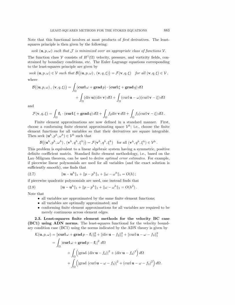
LEAST-SQUARES METHODS FOR THE STOKES EQUATIONS 883
Note that this functional involves at most products of first derivatives. The least-squares principle is then given by the following:
seek (u, p, ω) such that J is minimized over an appropriate class of functions V.
The function class V consists of H1(Ω) velocity, pressure, and vorticity fields, con-strained by boundary conditions, etc. The Euler–Lagrange equations correspondingto the least-squares principle are given by
seek (u, p, ω) ∈ V such that B((u, p, ω) , (v, q, ξ))
= F(v, q, ξ) for all (v, q, ξ) ∈ V ,where
B((u, p, ω) , (v, q, ξ))
=
∫Ω
(curlω + grad p) · (curl ξ + grad q) dΩ
+
∫Ω
(div u)(div v) dΩ +
∫Ω
(curl u− ω)(curl v − ξ) dΩ
and
F(v, q, ξ) =
∫Ω
f1 · (curl ξ + grad q) dΩ +
∫Ω
f2div v dΩ +
∫Ω
f3(curl v − ξ) dΩ .
Finite element approximations are now defined in a standard manner. First,choose a conforming finite element approximating space Vh; i.e., choose the finiteelement functions for all variables so that their derivatives are square integrable.Then seek (uh, ph, ωh) ∈ Vh such that
B((uh, ph, ωh) , (vh, qh, ξh))
= F(vh, qh, ξh) for all (vh, qh, ξh) ∈ Vh .This problem is equivalent to a linear algebraic system having a symmetric, positivedefinite coefficient matrix. Standard finite element methodology, i.e., based on theLax–Milgram theorem, can be used to derive optimal error estimates. For example,if piecewise linear polynomials are used for all variables (and the exact solution issufficiently smooth), one finds that
(2.7) ‖u− uh‖1 + ‖p− ph‖1 + ‖ω − ωh‖1 = O(h) ;
if piecewise quadratic polynomials are used, one instead finds that
(2.8) ‖u− uh‖1 + ‖p− ph‖1 + ‖ω − ωh‖1 = O(h2) .
Note that• all variables are approximated by the same finite element functions;• all variables are optimally approximated; and• conforming finite element approximations for all variables are required to be
merely continuous across element edges.
2.3. Least-squares finite element methods for the velocity BC case(BC1) using ADN norms. The least-squares functional for the velocity bound-ary condition case (BC1) using the norms indicated by the ADN theory is given by
K(u, p, ω) = ‖curlω + grad p− f1‖20 + ‖div u− f2‖21 + ‖curl u− ω − f3‖21=
∫Ω
|curlω + grad p− f1|2 dΩ
+
∫Ω
(|grad (div u− f2)|2 + (div u− f2)
2)dΩ
+
∫Ω
(|grad (curl u− ω − f3)|2 + (curl u− ω − f3)
2)dΩ .

884 JENNIFER M. DEANG AND MAX D. GUNZBURGER
Note that this functional involves products of second derivatives of the velocity. Theleast-squares principle is then given by the following:
seek (u, p, ω) such that K is minimized over an appropriate class of functions W.
The function class W now consists of H1(Ω) pressure and vorticity fields and H2(Ω)velocity fields, constrained by boundary conditions, etc. The Euler–Lagrange equationfor this least-squares principle again has the form
seek (u, p, ω) ∈ W such that B((u, p, ω) , (v, q, ξ))
= F(v, q, ξ) for all (v, q, ξ) ∈ W ,
where B(·, ·) is a bilinear form that involves products of second derivatives of u andv.
Finite element approximations can then be defined in a standard manner as fol-lows. First, choose a conforming finite element approximating space Wh; i.e., choosethe finite element functions for approximating the pressure and vorticity so that theirderivatives are square integrable and choose finite element functions for approximat-ing the velocity so that their second derivatives are square integrable. Then seek(uh, ph, ωh) ∈ Wh such that
B((uh, ph, ωh) , (vh, qh, ξh))
= F(vh, qh, ξh) for all (vh, qh, ξh) ∈ Wh .
This problem is again equivalent to a linear algebraic system having a symmetric,positive definite coefficient matrix. Standard finite element methodology, i.e., basedon the Lax–Milgram theorem, can be used to derive optimal error estimates wheneverconforming finite element spaces are used.
Unfortunately, this method for the velocity boundary condition (BC1) is not prac-tical. The requirement that finite element velocity approximations possess two squareintegrable derivatives forces one to use finite element functions that are continuouslydifferentiable across element edges. By the way, if one is willing to use continuouslydifferentiable velocity approximations, one might as well have applied least-squaresprinciples to the primitive variable formulation (2.1)–(2.3)!
2.4. A practical least-squares finite element method for the velocityBC case (BC1). At this point we are faced with the following scenario.
• The dilemma:– If, for the velocity boundary condition case (BC1), we use a least-squares
functional based on the ADN norms, we are led to a computationalmethod requiring continuously differentiable velocity approximations;i.e., =⇒ we get an impractical method.
– If, on the other hand, we use the more practical functional J that workseasily and optimally for the normal velocity-pressure boundary condi-tions, =⇒we get nonoptimal approximations.
• The question– Is there a way to use the simpler and more practical norms of the func-
tional J and still get optimally accurate approximations?• The answer:
– It can be done if one uses mesh-dependent weights in the least-squaresfunctional.
The residual norms of the equations that, for practical reasons, we would like to useare given by
(2.9) ‖curlω + grad p− f1‖0 , ‖div u− f2‖0 , and ‖curl u− ω − f3‖0 ;

LEAST-SQUARES METHODS FOR THE STOKES EQUATIONS 885
the residual norms that, for mathematical reasons, the ADN theory would like us touse are given by
(2.10) ‖curlω + grad p− f1‖0 , ‖div u− f2‖1 , and ‖curl u− ω − f3‖1 .We will introduce weights so that the second and third residuals using the practicalnorms of (2.9) can be used instead of the corresponding impractical norms of (2.10).
In order to motivate the choice of weights in the practical least-squares functional,we need to recall the notion of inverse inequalities for finite element spaces; see, e.g.,[49]. The inverse inequality relevant to our discussion is
‖qh‖1 ≤ Ch−1‖qh‖0 ,where h is an appropriate measure of the grid size and qh is a function belonging toa regular finite element subspace of H1(Ω). This inequality suggests that, for finiteelement functions, one can “simulate” the norm ‖qh‖1 by h−1‖qh‖0 .
Thus, we are led to the weighted least-squares functional for the velocity boundarycondition case (BC1):
Jh(u, p, ω) = ‖curlω + grad p− f1‖20 + h−2‖div u− f2‖20 + h−2‖curl u− ω − f3‖20=
∫Ω
|curlω + grad p− f1|2 dΩ +1
h2
∫Ω
(div u− f2)2dΩ
+1
h2
∫Ω
(curl u− ω − f3)2dΩ .
The least-squares principle is now given by the following:
seek (u, p, ω) such that Jh is minimized over an appropriate class of functions V.
The function class V again consists of H1(Ω) velocity, pressure, and vorticity fields,constrained by boundary conditions, etc. The Euler–Lagrange equations correspond-ing to this least-squares principle are given by
seek (u, p, ω) ∈ V such that Bh((u, p, ω) , (v, q, ξ)
)= Fh(v, q, ξ) for all (v, q, ξ) ∈ V ,
where
Bh((u, p, ω) , (v, q, ξ)
)=
∫Ω
(curlω + grad p) · (curl ξ + grad q) dΩ
+1
h2
∫Ω
(div u)(div v) dΩ +1
h2
∫Ω
(curl u− ω)(curl v − ξ) dΩ
and
Fh(v, q, ξ) =
∫Ω
f1 · (curl ξ+grad q) dΩ +1
h2
∫Ω
f2div v dΩ +1
h2
∫Ω
f3(curl v− ξ) dΩ .
Finite element approximations are now defined in a standard manner. First,choose a conforming finite element approximating space Vh; i.e., choose the finiteelement functions for all variables so that their derivatives are square integrable.Then seek (uh, ph, ωh) ∈ Vh such that
Bh((uh, ph, ωh) , (vh, qh, ξh)
)= Fh(vh, qh, ξh) for all (vh, qh, ξh) ∈ Vh .
This problems is equivalent to a linear algebraic system having a symmetric, positivedefinite coefficient matrix.

886 JENNIFER M. DEANG AND MAX D. GUNZBURGER
This method was analyzed in [11]. These analyses suggest that one may use poly-nomials of one degree lower for the pressure and vorticity than one uses for the velocity.If we use continuous piecewise quadratic polynomials for the velocity approximationsand piecewise linear polynomials for the pressure and vorticity approximations, weget the estimate
(2.11) ‖u− uh‖1 + ‖p− ph‖0 + ‖ω − ωh‖0 = O(h2) .
This estimate is optimal with respect to the finite element functions used. The theoryalso says that one may use the same degree polynomials for all variables. For example,if one uses continuous piecewise quadratic polynomials for all variables, one againobtains the above error estimate. In this case, the above estimate is not optimal forthe pressure and vorticity.
Thus, we are again led to a simple, easy-to-implement algorithm; i.e.,• one can use merely continuous finite element functions for all variables;• one still obtains a symmetric, positive definite discrete linear system; and• one obtains optimally accurate approximations. However, optimal accuracy
is achieved with respect to norms dictated by the ADN theory for the velocityboundary condition case.
2.5. Other first-order formulations for the Stokes equations. The velocity-vorticity-pressure formulation is not the only possible first-order formulation for theStokes problem (2.1)–(2.3). Another possibility is the velocity-pressure-stress formu-lation. Although this formulation involves more unknowns than does the velocity-vorticity-pressure formulation, it has the advantage that the components of the stresstensor are computed directly. In the velocity-vorticity-pressure formulation, the stresstensor is recovered by differentiating the components of the velocity vector. Least-squares finite element methods based on the velocity-pressure-stress formulation areconsidered in [13]. A third first-order formulation for the Stokes equations is discussedin [33].
In [8] and [20], a least-squares finite element method for the Stokes and Navier–Stokes equations with velocity boundary conditions was introduced that, withoutthe need of introducing mesh-dependent weights, results in a least-squares functionalemploying only L2(Ω)-norms. This method is based on the velocity-pressure-gradientof velocity formulation given by the differential equations
U − (∇u)T = 0 in Ω ,
−(∇ · U)T + grad p = f in Ω ,
div u = 0 in Ω ,
grad (traceU) = 0 in Ω ,
and
∇× U = 0 in Ω
and boundary conditions
u = 0 on Γ
LEAST-SQUARES METHODS FOR THE STOKES EQUATIONS 887
and
n× U = 0 on Γ .
The unknown fields is the nonsymmetric tensor U , the vector u, and the scalar p.Although this method is of considerable theoretical importance, its practical impactmay be limited. An obvious disadvantage of the method is that, in three dimensions,it requires 13 unknowns fields as opposed to 7 fields for the velocity-vorticity-pressureformulation. On the other hand, in principle, one does not have to introduce anymesh-dependent weights in order to get a viable discretization method. However, thisobservation is valid only for simple problems or for mesh sizes that are too smallto be used in practice. In section 3, we will often find that when complications areintroduced into a problem that mesh-dependent weights can serve to also amelioratethe impact of those complications. Thus, it seems likely that mesh-dependent weightswill be part of practical implementations of any least-squares finite element methodfor the Stokes or Navier–Stokes equations. For this reason, and also because least-squares finite element methods based on the velocity-vorticity-pressure formulationare by far the most used in engineering practice, we will concentrate on practicalissues connected with the implementation of that method.
3. Computational study of practical implementation issues. We now con-sider a series of issues that arise when least-squares finite element methods are usedin practical settings. These issues relate to settings which are, for the most part,not covered by existing theories. Since the issues we discuss are not related to thenonlinearity of the Navier–Stokes equations and are not peculiar to three-dimensionalgeometries, we will use the generalized velocity-vorticity-pressure formulation of thetwo-dimensional Stokes equations given by (2.4)–(2.6) as the basis for our computa-tional studies.
Unless otherwise noted, the results we report on are for the exact solution
(3.1) u = v = sin(πx) sin(πy) ,
(3.2) ω = sin(πx) exp(πy) ,
and
(3.3) p = cos(πx) exp(πy) .
The data functions f1, f2, and f3 are determined by substituting (3.1)–(3.3) into(2.4)–(2.6).
Possibly inhomogeneous versions of the two types of boundary conditions (BC1)and (BC2) are considered; furthermore, we will also examine cases for which theseboundary conditions are applied on disjoint parts of the boundary Ω. Thus, if ΓBC1
and ΓBC2 denote two disjoint parts of the boundary Γ such that ΓBC1 ∪ ΓBC2 = Γ,we specify the boundary conditions
(BC1) u = U on ΓBC1
and
(BC2) u · n = Un and p = P on ΓBC2

888 JENNIFER M. DEANG AND MAX D. GUNZBURGER
Table 1Convergence rates for quadratic-quadratic approximations.
L2 error rates H1 error ratesFunction BC1 BC1w BC2 BC2w BC1 BC1w BC2 BC2w
u 2.61 3.76 3.14 3.10 1.90 2.19 2.04 2.04v 2.34 3.32 3.13 3.09 2.02 2.13 2.02 2.02w 2.10 3.52 3.00 2.94 1.57 2.39 1.91 1.90p 2.41 3.22 2.97 2.97 1.57 2.40 1.96 1.96
for a given vector-valued function U defined on ΓBC1 and given functions Un andP defined on ΓBC2. If Γ = ΓBC1, then, for the solution to be unique, an additionalconstraint must be imposed on the pressure such as requiring the pressure to have zeromean over Ω. The boundary condition (BC2) is not necessarily useful in the contextof viscous flows; we consider it here merely to compare and contrast the behavior ofleast-squares finite element methods for each of the two boundary conditions (BC1)and (BC2). Whenever inhomogeneous boundary conditions are applied, interpolantsof the given data in the corresponding finite element spaces are used. The use ofinterpolants does not seem to affect the convergence behavior of the approximations.
Unless otherwise noted, all our computations are for a unit square domain, i.e.,Ω = (0, 1)× (0, 1). Note that in this case we have, for the exact solution (3.1)–(3.3),that U = 0 and Un = 0. In all cases, Ω is subdivided into triangular finite elements.Unless otherwise noted, uniform grids are used. The calculations for the unit squaredomain are done on a sequence of n× n grids with n = 2, 3, . . . , 20. Using the resultsfrom all these grids, a linear regression is used to calculate rates of convergence. Someof the reported rates of convergence are well above the optimal rates; this is probablydue to the fact that the linear regressions used to calculate the rates include calculatedresults obtained on coarse grids. However, for the calculations reported on here, wehave found this method for computing rates to be more reliable than using only thetwo finest grids, i.e., n = 19 and 20, or using the two finest nested grids, i.e., n = 10and 20.
We will study least-squares finite element methods based on both the weightedand unweighted functionals J and Jh, respectively. Whenever the weighted functionalis used, we will append a “w” to the boundary conditions designator; e.g., if we usethe weighted functional with boundary condition BC1, we will denote that case byBC1w.
3.1. Quadratic-quadratic finite element spaces. In this section, we use con-tinuous piecewise quadratic polynomials for all four variables, i.e., for the two compo-nents of the velocity, the vorticity, and the pressure. The use of a single approximatingspace for all variables simplifies programming of least-squares finite element methods.The computational results are obtained for the exact solution (3.1)–(3.3) on a unitsquare domain. In Table 1 are listed rates of convergence (with respect to the gridsize) determined from errors computed on different grids for various combinations ofboundary conditions and functionals.
We first study the case for which the boundary condition (BC2) is applied on allof Γ and for which we use the functional J as the basis for the least-squares finiteelement method. In this case, with the use of quadratic finite element functions forall four variables, one expects from (2.8) that the approximations to all four variablesconverge at a second-order rate in the H1-norm. This is confirmed by the resultslisted in the BC2 columns of Table 1. Note also the third-order rate for the error

LEAST-SQUARES METHODS FOR THE STOKES EQUATIONS 889
measured in the L2-norm.Next, we stay with the boundary condition (BC2) applied on all of Γ, but now
we use the weighted functional Jh as the basis for the least-squares finite elementmethod. This case is not covered by the theories of section 2. However, we see fromthe BC2w columns of Table 1 that the accuracy of the approximations for this caseis nearly the same as for the previous case wherein we used (BC2) on all of Γ alongwith the functional J . Thus, the use of mesh-dependent weights does not seem toaffect the accuracy of quadratic-quadratic approximations for the case (BC2).
Now we turn to cases for which the boundary condition (BC1) is applied on allof the boundary. The theories of section 2 do not apply to this boundary conditionif one uses the unweighted functional J . From the BC1 columns of Table 1, one seesthat the rates of convergence for this combination are not all optimal. The H1-normrates are probably more reliable indicators of what happens in general. There we seethat there is a slight loss of accuracy for the vorticity and pressure approximations;i.e., one does not recover the full second-order accuracy of the quadratic finite elementfunctions used.
If instead we use the weighted functional Jh along with the boundary condition(BC1) on all of Γ, the theory of section 2.4 results in the error estimate (2.11). Thus,the error estimate predicts that one obtains optimal second-order convergence forvelocity approximations in the H1-norm. For vorticity and pressure approximations,this estimate only predicts that the L2-norm convergence rates are no worse thansecond-order, which is suboptimal for the quadratic finite element functions used.However, from the BC1w columns of Table 1, we see that one does better than thatfor the vorticity and pressure.
The conclusion that can be reached is that the use of quadratic finite elementfunctions for all variables yields optimal accurate approximations whenever (BC1) or(BC2) is applied on all of the boundary, so long as the weighted functional is used forthe case (BC1).
3.2. Quadratic-linear finite element spaces. In Table 2, we give computedconvergence rates using continuous piecewise quadratic finite element functions forthe velocity component approximations and continuous piecewise linear finite elementfunctions for the vorticity and pressure approximations. The error estimates (2.11)for the case BC1w were valid for quadratic or linear approximations of the vorticityand pressure. As previously noted in Table 1, using quadratic approximations for pand ω yields a higher rate of convergence for BC1w than predicted by (2.11). Theuse of linear approximations for the vorticity and pressure should mimic more closelythe theoretical result (2.11) for the BC1w case. In fact, examination of the BC1wcolumns in Table 2 indicates that indeed the H1 errors of the velocity componentsand the L2 errors of the vorticity and pressure are all of O(h2), as predicted by (2.11).The H1 rate of convergence for the vorticity and pressure approximations seems tobe optimal for the linear functions used for these variables.
Looking at the BC1 columns of Table 2, we see that using quadratic approxima-tions for the velocity and linear approximations for the vorticity and pressure resultsin a disastrous loss of accuracy with respect to both the H1 and L2 errors. The BC2and BC2w columns are nearly identical; they indicate that the accuracy is severelycompromised, especially for the quadratic velocity approximations.
The conclusion that can be drawn from Table 2 is that quadratic-linear approxi-mations can only be used in the BC1w case for which the theory leading to the errorestimate (2.11) applies. Otherwise, one gets substantially less accuracy than possible
890 JENNIFER M. DEANG AND MAX D. GUNZBURGER
Table 2Convergence rates for quadratic-linear approximations.
L2 error rates H1 error ratesFunction BC1 BC1w BC2 BC2w BC1 BC1w BC2 BC2w
u 0.12 2.00 0.92 0.92 0.14 1.91 1.03 1.02v 0.15 2.54 0.92 0.91 0.14 2.18 1.08 1.08w 0.17 2.01 1.14 1.13 0.16 1.22 0.91 0.91p 0.29 1.98 1.96 1.96 0.16 1.21 0.91 0.96
Table 3Convergence rates for linear-linear approximations.
L2 error rates H1 error ratesFunction BC1 BC1w BC2 BC2w BC1 BC1w BC2 BC2w
u 0.24 1.83 1.25 0.82 0.17 1.12 0.93 0.78v 0.29 2.08 1.29 0.87 0.12 1.13 0.93 0.79w 0.19 2.01 1.49 0.83 0.17 1.20 0.91 0.88p 0.22 1.66 1.96 1.96 0.17 1.19 0.96 0.96
with the finite element functions used.
3.3. Linear-linear finite element spaces. The theory for the pressure-normalvelocity boundary condition (BC2) and the unweighted functional J that led to theerror estimate (2.7) applies to continuous piecewise linear velocity approximationsalong with like approximations for the vorticity and pressure. However, the theoryfor the velocity boundary condition and the weighted functional Jh that led to theerror estimate (2.11) does not apply to this choice of approximating functions for thevelocity. Thus, our next computational study is to determine convergence rates forthis linear-linear case and for the various combinations of boundary conditions andfunctionals. The results are given in Table 3.
Very poor rates result when the boundary condition (BC1) is combined withthe unweighted functional J . Use of the weighted functional Jh seems to yield goodconvergence rates; indeed, with respect to the H1-norm these seem to be optimal. Therates for the boundary condition (BC2) combined with the unweighted functional Jconfirm the theoretical results of (2.7). In this case, it seems that the use of weightshurts the accuracy of the approximations for the normal velocity-pressure boundarycondition case.
The conclusion that can be drawn from these results is that linear approximationsfor the velocity may be safely used for the boundary condition (BC1) so long asthe weighted functional is used. For the boundary condition (BC2), the unweightedfunctional performs better than the weighted one; however, the latter can still besafely used.
3.4. Mixed boundary conditions. The next series of computations studiesthe effects of using the two boundary conditions (BC1) and (BC2) simultaneously ondifferent parts of the boundary. Four different configurations, as depicted in Figure 1,of mixed boundary conditions were implemented. The ADN theory is a local theory;i.e., it deals with behavior in the neighborhood of points on the boundary and does notapply to mixed boundary condition cases. The computational experiments using thedistributions of boundary conditions depicted in Figure 1 are therefore of interest tosee how least-squares methods based on both the unweighted and weighted functionalsperform in such settings.

LEAST-SQUARES METHODS FOR THE STOKES EQUATIONS 891
Fig. 1. Distribution of boundary conditions; solid line for BC1, dashed line for BC2.
Table 4Convergence rates for quadratic-quadratic approximations with mixed boundary conditions.
L2 error ratesUnweighted functional Weighted functional
Function Case 1 Case 2 Case 3 Case 4 Case 1 Case 2 Case 3 Case 4u 2.88 2.45 2.97 1.95 2.99 3.65 3.07 3.52v 2.97 2.49 3.15 1.98 3.09 3.40 3.20 3.37w 2.48 2.11 2.75 1.81 2.90 3.35 3.09 3.50p 2.58 1.95 2.69 1.81 3.04 3.29 3.11 3.48
H1 error ratesUnweighted functional Weighted functional
Function Case 1 Case 2 Case 3 Case 4 Case 1 Case 2 Case 3 Case 4u 2.01 1.84 2.02 1.90 2.01 2.16 2.01 2.06v 2.01 2.10 2.03 1.75 2.01 2.17 2.01 2.14w 1.91 1.57 1.94 1.64 1.90 2.39 1.93 2.22p 1.96 1.58 1.98 1.65 1.96 2.40 1.98 2.24
All four mixed boundary condition cases were approximated using both the un-weighted functional J and the weighted functional Jh. In Table 4, we give computedconvergence rates in the L2- and H1-norms using continuous piecewise quadratic fi-nite element functions for the approximation of all variables. We see that use of theweighted functional yields optimal convergence rates for all four cases. However, useof the unweighted functional results in suboptimal H1 rates for Cases 2 and 4. It alsoseems that suboptimal L2 rates are attained for all four cases, with again Cases 2 and4 yielding the worst results.
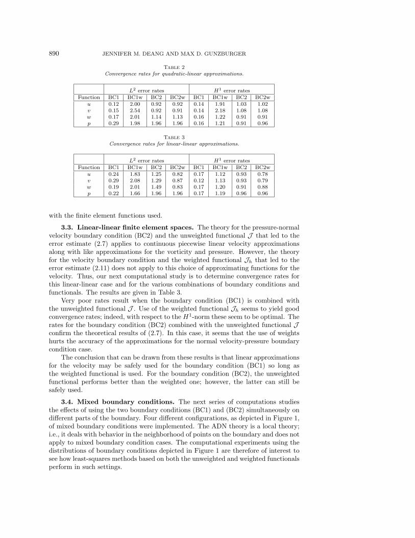
In Table 5, we give computed convergence rates in the L2- and H1-norms usingcontinuous piecewise quadratic finite element functions for the velocity approximationand continuous piecewise linear finite element functions for the vorticity and pressure.We see that use of the unweighted functional yields severely suboptimal convergencerates for all four cases. Use of the weighted functional results in much improvedapproximations, although fully optimal approximations are only obtained for Case 3.In this table, the rates for u seem to differ more widely from those for v than in mostof the other tables; we do not have an explanation for this phenomena.
In Table 6, we give computed convergence rates in the L2- and H1-norms using
892 JENNIFER M. DEANG AND MAX D. GUNZBURGER
Table 5Convergence rates for quadratic-linear approximations with mixed boundary conditions.
L2 error ratesUnweighted functional Weighted functional
Function Case 1 Case 2 Case 3 Case 4 Case 1 Case 2 Case 3 Case 4u 1.72 0.42 1.08 0.00 1.88 2.19 3.03 1.29v 1.79 0.17 1.35 0.29 1.94 2.50 2.87 1.75w 1.67 0.30 1.07 0.29 1.82 2.06 2.39 1.60p 1.66 0.31 1.18 0.18 1.95 1.94 2.60 1.34
H1 error ratesUnweighted functional Weighted functional
Function Case 1 Case 2 Case 3 Case 4 Case 1 Case 2 Case 3 Case 4u 1.58 0.40 0.96 0.14 1.63 2.04 2.30 1.35v 1.61 0.14 1.29 0.35 1.78 2.15 2.35 1.60w 0.90 0.20 0.95 0.30 0.91 1.23 1.12 0.93p 0.96 0.20 0.96 0.43 0.96 1.21 1.15 0.97
continuous piecewise linear finite element functions for the approximation of all vari-ables. For Case 1, one sees that the use of the unweighted functional results in slightlybetter convergence rates than does use of the weighted functional; however, for Cases2, 3, and 4, use of the weighted functional results in substantially better convergencerates than does use of the unweighted functional.
The following conclusions can be inferred from our computational experiments.In most cases, use of the weighted functional yields better results, and in all casesit yields “decent” rates of convergence. The unweighted functional can at best besafely used only in Cases 1 and 3; otherwise, serious loss of accuracy occurs. Oneshould note that in Cases 1 and 3 the boundary condition (BC2) is applied on partsof the boundary that are aligned with both coordinate axes while in Cases 2 and 4that boundary condition is applied only on parts of the boundary that are alignedwith a single coordinate axis. One may infer from this the following rule of thumb:the unweighted functional can be safely used (in the sense that any loss of accuracywill not be disastrous) only if the boundary condition (BC2) is applied on parts ofthe boundary whose normal vectors span R2. On the other hand, it seems that theweighted functional can be safely used in all cases.
3.5. Mass conservation. Mass conservation, i.e., the satisfaction of the conti-nuity equation, is often a paramount concern of users of computational fluid dynamicalgorithms. In [43], it was reported that least-squares finite element methods of thetype discussed so far do a very poor job at conserving mass, and a remedy was pro-posed. Unfortunately, this remedy, which consists of enforcing the continuity equationas an explicit constraint through the use of Lagrange multipliers, defeats one of themain purposes of using least-squares methods! Indeed, one loses the positive defi-niteness resulting from the least-squares formulation and is led to indefinite problemssimilar to those that arise in standard mixed-Galerkin methods for the Stokes prob-lem!
Here, we explore, through some computational experiments, the seriousness ofthe lack of mass conservation in least-squares finite element methods for the Stokesproblem. First, we examine the generalized Stokes problem (2.4)–(2.6) with the exactsolution (3.1)–(3.3); then we examine the specific problem discussed in [43].
One advantage of least-squares methodologies for systems of equations is that onecan, through the introduction of weights, enhance the importance of any equation or

LEAST-SQUARES METHODS FOR THE STOKES EQUATIONS 893
Table 6Convergence rates for linear-linear approximations with mixed boundary conditions.
L2 error ratesUnweighted functional Weighted functional
Function Case 1 Case 2 Case 3 Case 4 Case 1 Case 2 Case 3 Case 4u 1.65 0.36 0.78 0.50 0.75 1.77 1.36 1.47v 1.70 0.32 0.97 0.55 0.82 2.00 1.43 1.36w 1.62 0.30 1.01 0.28 0.85 1.92 1.92 1.49p 1.59 0.32 1.14 0.19 1.77 1.94 2.30 1.40
H1 error ratesUnweighted functional Weighted functional
Function Case 1 Case 2 Case 3 Case 4 Case 1 Case 2 Case 3 Case 4u 0.95 0.32 0.75 0.54 0.78 1.16 1.08 0.95v 0.94 0.13 1.00 0.34 0.81 1.13 1.00 0.94w 0.90 0.20 0.89 0.30 0.89 1.20 1.03 0.94p 0.96 0.20 0.91 0.35 0.96 1.20 1.08 0.98
equations (at the expense of the remaining ones, of course.) Thus, if one is interestedin enhancing mass conservation, one can use the functional
(3.4)Js,K(u, p, ω) =‖curlω + grad p− f1‖20
+Kh−s‖div u− f2‖20 + h−s‖curl u− ω − f3‖20with a “large” value for the positive weight K. Note that in terms of the notation wehave previously used, J = J0,1 and Jh = J2,1.
For the exact solution (3.1)–(3.3), in Table 7, we first give the residual ‖div uh −f2‖0 for a 10× 10 uniform grid for different values of K and s and for the two typesof boundary conditions (BC1) and (BC2), where uh denotes the approximate velocityfield. As before, in the table, BC1 and BC2 refer to the use of the functional (3.4)without mesh-dependent weights, i.e., with s = 0, and BC1w and BC2w refer to theuse of the functional (3.4) with mesh-dependent weights, i.e., with s = 2. Piecewisequadratic approximations are used for all variables. In Table 7, we also give the ratesof convergence for ‖div uh − f2‖0.
The column with K = 1 corresponds to our previous calculations; i.e., no specialtreatment of the continuity equation is used. The columns with K > 1 correspond toincreasing the importance of that equation relative to the remaining ones, while thecolumns with K < 1 correspond to the opposite situation; i.e., the importance of thecontinuity equation is reduced relative to the other equations.
From the K = 1 column, we see, at least for this example, that mass conservationis accomplished to within the expected discretization error. Certainly the rates ofconvergence are what one expects. If there is any problem, it is with the use of theunweighted functional with the boundary condition (BC1). From the other columnswe see that choosing K > 1 has little effect except for the case just mentioned; thisis probably due to the fact that the residuals are already well within discretizationerror for the other cases. Choosing K < 1, however, can result in a deterioration inthe mass conserving ability of the schemes.
We now consider a problem similar to that discussed in [43]. We solve the Stokessystem (2.4)–(2.6) with f1 = 0, f2 = 0, and f3 = 0; note that in this case div u = 0so that we have the usual continuity equation holding. The computational domain isthe rectangle [−5, 5] × [−5, 15] excluding a circle centered at (0, 0). On the sides ofthe rectangle, we impose the boundary conditions u = 1 and v = 0, where u and v

894 JENNIFER M. DEANG AND MAX D. GUNZBURGER
Table 7The residual ‖div uh − f2‖0 for h = 0.1 and its convergence rate for different values of the
weight parameter K, for the two boundary conditions (BC1) and (BC2), and for the mesh-weightedand unweighted functionals.
Residual for h = 0.1K .01 .1 1 10 100
BC1 1.3914 0.3838 0.0736 0.0255 0.0251BC1w 0.2004 0.0462 0.0247 0.0237 0.0251BC2 0.1357 0.0516 0.0286 0.0264 0.0299
BC2w 0.1348 0.0509 0.0285 0.0263 0.0300Convergence rates
K .01 .1 1 10 100BC1 1.36 1.79 2.02 2.03 2.03
BC1w 2.53 2.76 2.21 2.03 2.13BC2 1.58 2.14 2.15 2.13 2.15
BC2w 1.59 2.15 2.15 2.13 2.15
Fig. 2. Finite element grids for a circle of diameter 1.
denote the x- and y-components of the velocity; on the circle, we specify u = v = 0.Three different diameters, i.e., 1, 3, and 6, of the circle were used in the numerical
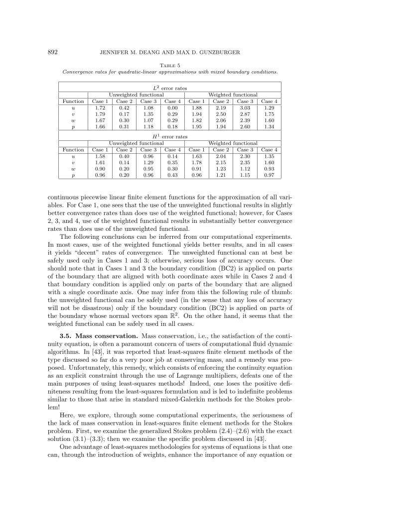
study; the grids used in the computations for the three cases are depicted in Figures 2–4, respectively. Note that the same number of grid points is used for all three cases,but, of course, they are redistributed due to the changing size of the circle. Piecewisequadratic approximations are used for all variables.
The amount of mass (assuming a unit density) entering on the left side and exitingfrom the right side of the rectangle is 10; due to symmetry, we expect that 5 units ofmass flows through each of the openings between the circle and the upper and lowersides of the rectangle. Since these openings are of size 4.5, 3.5, and 2 for each of thecircles of diameter 1, 3, and 6, respectively, and since the entrance and exit values ofthe horizontal velocities are 1, we expect that the average value of u along the verticalline segment at the minimum opening, i.e., at x = 0 and extending from the circle tothe nearest side of the rectangle, to be 10/9, 10/7, and 10/4, respectively.
Five different sets of computational experiments, corresponding to five choicesfor the least-squares functionals, were conducted. For Case i, we use the unweighted
LEAST-SQUARES METHODS FOR THE STOKES EQUATIONS 895
Fig. 3. Finite element grids for a circle of diameter 3.
functional J0,1 = J ; see (3.4) with f1 = 0, f2 = 0, and f3 = 0. For Case ii, we use themesh-weighted functional J2,1 = Jh, where h is chosen as an average grid size; againsee (3.4). For Case iii, we use the mesh and continuity equation-weighted functionalJ2,10, where again h is chosen as an average grid size. The last two cases use theleast-squares functional
(3.5)
Js,K(u, p, ω) =‖curlω + grad p− f1‖20+∑j
h−sj(K‖div u− f2‖20,∆j
+ ‖curl u− ω − f3‖20,∆j
),
where the sum is taken over the finite elements, ∆j denotes the jth finite element, hjdenotes the diameter of ∆j , and ‖ · ‖0,∆j
denotes the L2(∆j)-norm. The functionaldefined in (3.5) allows for mesh-dependent weighting that varies from triangle totriangle, while the functional defined in (3.4) only allows mesh-dependent weightingthat is fixed for all triangles. For Case iv, we use the locally mesh-weighted functionalJ2,1, while for Case v we use the locally mesh-weighted and continuity equation-
weighted functional J2,10.Results for the five different choices for the least-squares functional are given in
Table 8. The computed masses flowing through each of the openings between the circleand the upper and lower sides of the rectangle are compared, for all five cases andfor all three sizes for the circle, with its expected value. Also, the computed averagevalues of u along the vertical line segment at the minimum opening are comparedwith its expected values.
We see that for the small circle of diameter 1, i.e., for a relatively large openingabove and below the circle, that nearly the correct amount of mass and nearly thecorrect average velocity is achieved. However, as the opening becomes constricted,i.e., as the circle gets larger, mass conservation is less well achieved, especially for theunweighted functional of Case i. Adding mesh-dependent weights improves the situa-tion, although not as much as adding both mesh and continuity equation-dependentweights. There seems to be little difference between using global or local mesh-dependent weights.

896 JENNIFER M. DEANG AND MAX D. GUNZBURGER
Fig. 4. Finite element grids for a circle of diameter 6.
Table 8Mass passing above or below circle and average velocity along vertical line segment above or
below circle.
MassDiameter Expected Case i Case ii Case iii Case iv Case v
1 5 4.9469 4.9720 4.9918 4.9671 4.99183 5 4.9322 4.9556 4.9868 4.9511 4.98616 5 4.2634 4.5070 4.8936 4.4586 4.8868
Average velocityDiameter Expected Case i Case ii Case iii Case iv Case v
1 1.1111 1.0993 1.1049 1.1094 1.1038 1.10933 1.4285 1.4092 1.4159 1.4247 1.4146 1.42466 2.5000 2.1317 2.2535 2.44683 2.2293 2.4434
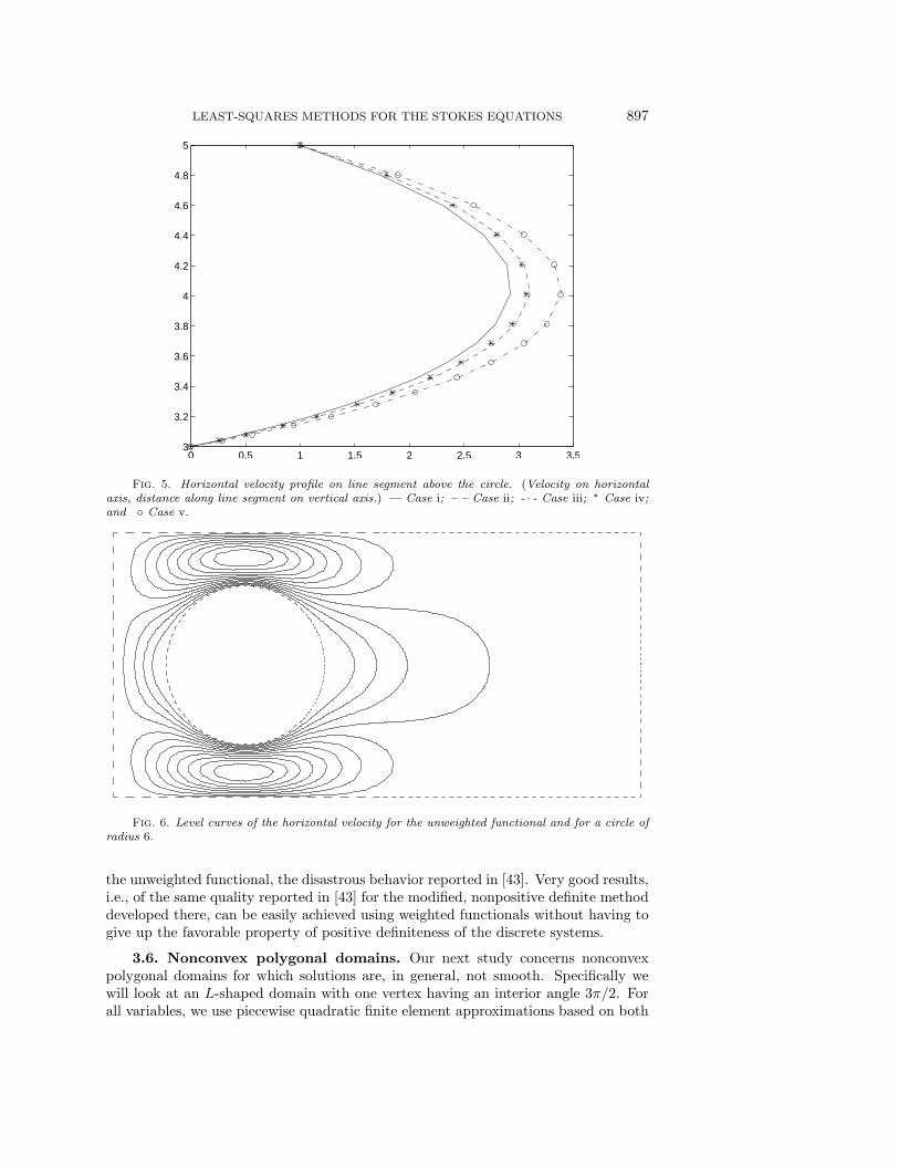
These observations are reinforced by Figure 5 in which are plotted horizontalvelocity profiles along the vertical line segment joining the top of the circle and theupper side of the rectangle. The profiles for all five cases are plotted for the circle ofdiameter 6, i.e., the configuration giving the poorest results in Table 8. In Figure 5,we see the worst result for the unweighted functional, improved results for locally orglobally mesh-dependent weighted functionals, and the best results for the mesh andcontinuity equation-dependent weighted functionals. Again, we also see that there islittle difference in the results for locally or globally mesh-weighted functionals.
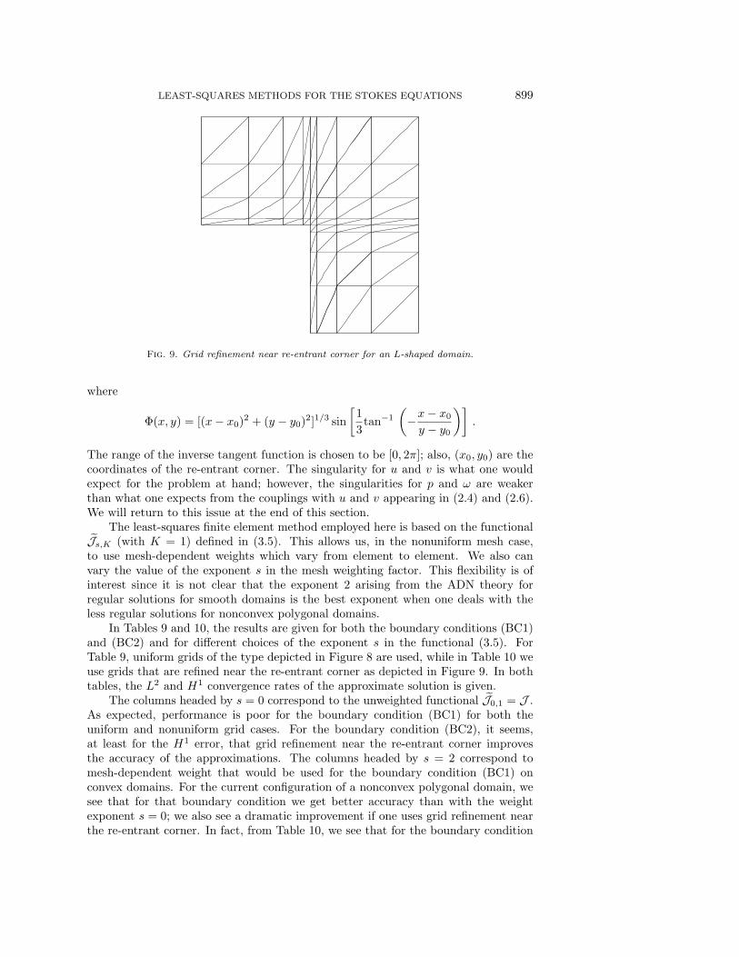
To finish our comparisons with the results of [43], in Figure 6 we give the levelcurves of the horizontal velocity component and, in Figure 7, a vector plot of thevelocity field. Both figures are for the worst combination of the unweighted functional,i.e., Case i, and a circle with diameter 6. Even in this worst-case scenario, which issimilar to that reported in [43], we do not find the poor mass conservation propertiesof least-squares finite element methods reported in that article. In fact, Figures 5, 6,and 7 are qualitatively the same as those for the modified method developed in [43]and which leads to nonpositive definite linear systems.
The following conclusions can be drawn from our studies of the mass conservationproperties of least-squares finite element methods. First, we do not observe, even for
LEAST-SQUARES METHODS FOR THE STOKES EQUATIONS 897
0 0.5 1 1.5 2 2.5 3 3.53
3.2
3.4
3.6
3.8
4
4.2
4.4
4.6
4.8
5
Fig. 5. Horizontal velocity profile on line segment above the circle. (Velocity on horizontalaxis, distance along line segment on vertical axis.) — Case i; – – Case ii; - · - Case iii; ∗ Case iv;and Case v.
Fig. 6. Level curves of the horizontal velocity for the unweighted functional and for a circle ofradius 6.
the unweighted functional, the disastrous behavior reported in [43]. Very good results,i.e., of the same quality reported in [43] for the modified, nonpositive definite methoddeveloped there, can be easily achieved using weighted functionals without having togive up the favorable property of positive definiteness of the discrete systems.
3.6. Nonconvex polygonal domains. Our next study concerns nonconvexpolygonal domains for which solutions are, in general, not smooth. Specifically wewill look at an L-shaped domain with one vertex having an interior angle 3π/2. Forall variables, we use piecewise quadratic finite element approximations based on both

898 JENNIFER M. DEANG AND MAX D. GUNZBURGER
Fig. 7. The velocity field for the unweighted functional and for a circle of radius 6.
Fig. 8. Uniform grid for an L-shaped domain.
uniform meshes and meshes refined in the neighborhood of the re-entrant corner. SeeFigures 8 and 9 for examples of such grids as well as for the shape of the domain weare considering. For the calculations reported here, the number of grid points usedalong the longest sides of the L-shaped domain were chosen to be 2, 4, 6, . . . , 20.
In order to partially mimic the singularity in the solution that results from ap-plying velocity conditions on the edges meeting at the re-entrant corner, we consider,instead of (3.1)–(3.3), the exact solution
(3.6)
u = v = Φ(x, y) + sin(πx) sin(πy),
p = Φ(x, y) + cos(πx) expπy,
ω = Φ(x, y) + sin(πx) expπy ,
LEAST-SQUARES METHODS FOR THE STOKES EQUATIONS 899
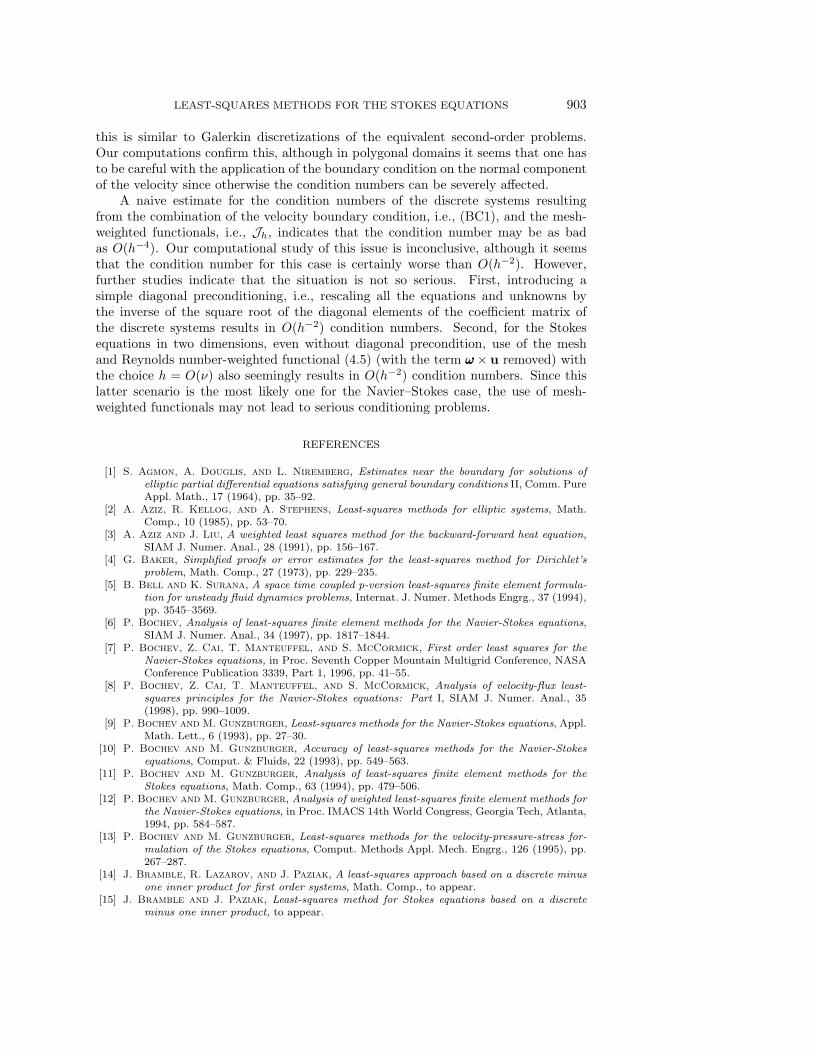
Fig. 9. Grid refinement near re-entrant corner for an L-shaped domain.
where
Φ(x, y) = [(x− x0)2 + (y − y0)2]1/3 sin
[1
3tan−1
(−x− x0
y − y0
)].
The range of the inverse tangent function is chosen to be [0, 2π]; also, (x0, y0) are thecoordinates of the re-entrant corner. The singularity for u and v is what one wouldexpect for the problem at hand; however, the singularities for p and ω are weakerthan what one expects from the couplings with u and v appearing in (2.4) and (2.6).We will return to this issue at the end of this section.
The least-squares finite element method employed here is based on the functionalJs,K (with K = 1) defined in (3.5). This allows us, in the nonuniform mesh case,to use mesh-dependent weights which vary from element to element. We also canvary the value of the exponent s in the mesh weighting factor. This flexibility is ofinterest since it is not clear that the exponent 2 arising from the ADN theory forregular solutions for smooth domains is the best exponent when one deals with theless regular solutions for nonconvex polygonal domains.
In Tables 9 and 10, the results are given for both the boundary conditions (BC1)and (BC2) and for different choices of the exponent s in the functional (3.5). ForTable 9, uniform grids of the type depicted in Figure 8 are used, while in Table 10 weuse grids that are refined near the re-entrant corner as depicted in Figure 9. In bothtables, the L2 and H1 convergence rates of the approximate solution is given.
The columns headed by s = 0 correspond to the unweighted functional J0,1 = J .As expected, performance is poor for the boundary condition (BC1) for both theuniform and nonuniform grid cases. For the boundary condition (BC2), it seems,at least for the H1 error, that grid refinement near the re-entrant corner improvesthe accuracy of the approximations. The columns headed by s = 2 correspond tomesh-dependent weight that would be used for the boundary condition (BC1) onconvex domains. For the current configuration of a nonconvex polygonal domain, wesee that for that boundary condition we get better accuracy than with the weightexponent s = 0; we also see a dramatic improvement if one uses grid refinement nearthe re-entrant corner. In fact, from Table 10, we see that for the boundary condition

900 JENNIFER M. DEANG AND MAX D. GUNZBURGER
Table 9Convergence rates for a re-entrant corner problem with a uniform grid.
Uniform grid; boundary condition (BC1)
L2 error rates H1 error ratesFunction s = 0 s = 1 s = 1.5 s = 2 s = 0 s = 1 s = 1.5 s = 2
u 1.71 2.06 2.04 1.98 1.32 1.37 1.31 1.26v 2.02 2.04 1.94 1.87 1.40 1.35 1.29 1.25w 1.87 2.60 2.62 2.44 1.47 2.06 2.16 2.03p 1.68 2.48 1.09 1.63 1.47 2.06 2.18 2.09
Uniform grid; boundary condition (BC2)
L2 error rates H1 error ratesFunction s = 0 s = 1 s = 1.5 s = 2 s = 0 s = 1 s = 1.5 s = 2
u 1.58 1.52 1.33 0.94 1.17 1.17 1.13 0.94v 1.51 1.45 1.26 0.87 1.14 1.14 1.10 0.91w 2.21 1.49 0.93 0.42 1.85 1.83 1.72 1.41p 2.58 2.58 2.58 2.58 1.91 1.91 1.91 1.91
Table 10Convergence rates for re-entrant corner problem with a nonuniform grid.
Refined grid; boundary condition (BC1)
L2 error rates H1 error ratesFunction s = 0 s = 1 s = 1.5 s = 2 s = 0 s = 1 s = 1.5 s = 2
u 1.17 2.35 2.81 3.02 0.99 1.71 1.81 1.79v 1.26 2.28 2.72 2.92 1.15 1.77 1.81 1.79w 1.26 2.09 2.47 2.78 0.96 1.59 1.83 1.97p 1.01 2.01 2.39 2.36 0.96 1.59 1.82 1.96
Refined grid; boundary condition (BC2)
L2 error rates H1 error ratesFunction s = 0 s = 1 s = 1.5 s = 2 s = 0 s = 1 s = 1.5 s = 2
u 2.65 2.61 2.48 2.11 1.69 1.68 1.68 1.66v 2.58 2.54 2.39 2.02 1.65 1.65 1.64 1.62w 2.40 2.36 2.19 1.75 1.56 1.56 1.56 1.54p 2.44 2.44 2.44 2.44 1.61 1.61 1.61 1.61
(BC1), use of a locally mesh-dependent weight exponent s = 2 and grid refinementnear the re-entrant corner nearly recovers the optimal accuracy of the approximations.Overall, it seems that for the boundary condition (BC1) the best exponent s seemsto be somewhere between 1 and 2, while for the boundary condition (BC2) the bestexponent seems to be near 0.
One may be tempted to conclude from these very limited computational experi-ments that there is some hope of treating singularities arising from nonconvex polyg-onal domains in the least-squares finite element formalism by using mesh-dependentweights and local grid refinement near re-entrant corners. On the other hand, we havetried to compute with an example for which the ω in (3.6) is replaced with curl u,where u is chosen as in (3.6). For this case, we have obtained very poor results, evenwith grid refinement near the re-entrant corner and different choices for the mesh-dependent weight. More detailed studies are needed in order to ascertain the bestmesh weight exponents and grid refinement strategies.
4. Concluding remarks. We conclude with some brief remarks concerning thethree dimensional Stokes problem, the nonlinear Navier–Stokes equations, and thecondition numbers of the discrete systems. One other remark concerns the use of

LEAST-SQUARES METHODS FOR THE STOKES EQUATIONS 901
quadrature rules. We have found that even for quadratic approximations for all thevariables that the three-point midside rule for triangles is sufficiently accurate to pre-serve the discretization error of least-squares methods based on any of the functionalsinvolving only products of first-order derivatives, e.g., J and Jh. Indeed, results forthe three-point midside rule and a higher-order accurate seven-point rule for trianglesare virtually the same.
4.1. The Stokes equations in three dimensions. The velocity-vorticity-(total)-pressure formulation of the (generalized) Stokes equations with velocity bound-ary conditions in three dimensions is given by
(4.1)
curlωωω + grad p = f1
curl u− ωωω = f2
div u = f3
in Ω
and
(4.2) u = U on Γ .
Note that the vorticity is now vector valued. Thus, there are seven equations forthe seven scalar unknowns consisting of p and the components of u and ωωω. Thissystem cannot be elliptic. To remedy this, we add (see [39]) an extra variable φ anda seemingly redundant equation to get the elliptic system of eight equations in eightunknowns
(4.3)
curlωωω + grad p = f1
divωωω = −div f2
curl u + gradφ− ωωω = f2
div u = f3
in Ω
along with the boundary conditions
(4.4) u = U and φ = 0 on Γ .
It can easily be shown that φ = 0, so that solutions (u, ωωω, p) of (4.3)–(4.4) are indeedsolutions of (4.1)–(4.2).
Algorithmically, one can completely ignore φ, but one cannot ignore the redundantequation. Thus, one can discretize the problem
curlωωω + grad p = f1
divωωω = −div f2
curl u− ωωω = f2
div u = f3
in Ω
along with (4.2) using the weighted least squares functional
Jh(u, p,ωωω) = ‖curlωωω + grad p− f1‖20 + ‖divωωω + div f2‖20+ h−2‖curl u− ωωω − f2‖20 + h−2‖div u− f3‖20
=
∫Ω
|curlωωω + grad p− f1|2 dΩ +
∫Ω
(divωωω + div f2)2dΩ
+1
h2
∫Ω
(curl u− ωωω − f2)2dΩ +
1
h2
∫Ω
(div u− f3)2dΩ .
The analyses of the Stokes problems in three dimensions based on this functionalyields results identical to that obtained in the two-dimensional case.

902 JENNIFER M. DEANG AND MAX D. GUNZBURGER
4.2. The Navier–Stokes equations. The velocity-vorticity-(total)-pressure for-mulation of the Navier–Stokes equations with velocity boundary conditions in threedimensions is given by
νcurlωωω + ωωω × u + grad p = f
curl u− ωωω = 0
div u = 0
in Ω
and
u = U on Γ ,
where, if the equations are appropriately nondimensionalized, ν denotes the inverseof the Reynolds number. Computations and preliminary analyses indicate that thebest choice of least-squares functional for the Navier–Stokes equations is given by
(4.5)
Jh(u, p,ωωω) = ν−2‖νcurlωωω + grad p+ ωωω × u− f‖20 + ν−2‖divωωω‖20+ h−2‖curl u− ωωω‖20 + h−2‖div u‖20
=1
ν2
∫Ω
|νcurlωωω + grad p+ ωωω × u− f |2 dΩ +1
ν2
∫Ω
(divωωω)2dΩ
+1
h2
∫Ω
|curl u− ωωω|2 dΩ +1
h2
∫Ω
(div u)2dΩ.
Thus, in three dimensions we again add the redundant equation divωωω = 0; this doesnot apply in two dimensions. Note also that the vorticity transport equations and theredundant equations should be weighted with ν−2.
One must choose a method for linearizing the equation. If one uses Newton’smethod, then in the neighborhood of a solution, the Hessian matrix is not only sym-metric but is also positive definite.
Efficient computational solutions of the Navier–Stokes equations, especially atmoderate and high values of the Reynolds number, usually require the use of highlynonuniform grids, e.g., to resolve boundary layers. Thus, one might prefer to uselocally mesh-dependent weights in the least-squares functional.
In engineering practice, use of the unweighted (with respect to both the mesh andthe Reynolds number) functional
(4.6)J (u, p,ωωω) = ‖νcurlωωω + grad p+ ωωω × u− f‖20 + ‖divωωω‖20
+ ‖curl u− ωωω‖20 + ‖div u‖20has resulted in very high quality computational results. A possible explanation forthis paradox, i.e., that analyses seem to indicate that one should use the functional(4.5) while computations indicate that good results are obtained using the functional(4.6), is that if one chooses h = O(ν), then the functionals (4.5) and (4.6) differ onlyby an unimportant constant scale factor; it is indeed the case that one often choosesh to depend on ν, at least locally, e.g., in boundary layers.
4.3. Condition numbers for the discrete Stokes systems. For the least-squares finite element method based on the unweighted functional J in the case (BC2),i.e., normal velocity and pressure boundary conditions, it is easy to prove that thecondition numbers of the discrete systems of linear algebraic equations are O(h−2);
LEAST-SQUARES METHODS FOR THE STOKES EQUATIONS 903
this is similar to Galerkin discretizations of the equivalent second-order problems.Our computations confirm this, although in polygonal domains it seems that one hasto be careful with the application of the boundary condition on the normal componentof the velocity since otherwise the condition numbers can be severely affected.
A naive estimate for the condition numbers of the discrete systems resultingfrom the combination of the velocity boundary condition, i.e., (BC1), and the mesh-weighted functionals, i.e., Jh, indicates that the condition number may be as badas O(h−4). Our computational study of this issue is inconclusive, although it seemsthat the condition number for this case is certainly worse than O(h−2). However,further studies indicate that the situation is not so serious. First, introducing asimple diagonal preconditioning, i.e., rescaling all the equations and unknowns bythe inverse of the square root of the diagonal elements of the coefficient matrix ofthe discrete systems results in O(h−2) condition numbers. Second, for the Stokesequations in two dimensions, even without diagonal precondition, use of the meshand Reynolds number-weighted functional (4.5) (with the term ωωω × u removed) withthe choice h = O(ν) also seemingly results in O(h−2) condition numbers. Since thislatter scenario is the most likely one for the Navier–Stokes case, the use of mesh-weighted functionals may not lead to serious conditioning problems.
REFERENCES
[1] S. Agmon, A. Douglis, and L. Niremberg, Estimates near the boundary for solutions ofelliptic partial differential equations satisfying general boundary conditions II, Comm. PureAppl. Math., 17 (1964), pp. 35–92.
[2] A. Aziz, R. Kellog, and A. Stephens, Least-squares methods for elliptic systems, Math.Comp., 10 (1985), pp. 53–70.
[3] A. Aziz and J. Liu, A weighted least squares method for the backward-forward heat equation,SIAM J. Numer. Anal., 28 (1991), pp. 156–167.
[4] G. Baker, Simplified proofs or error estimates for the least-squares method for Dirichlet’sproblem, Math. Comp., 27 (1973), pp. 229–235.
[5] B. Bell and K. Surana, A space time coupled p-version least-squares finite element formula-tion for unsteady fluid dynamics problems, Internat. J. Numer. Methods Engrg., 37 (1994),pp. 3545–3569.
[6] P. Bochev, Analysis of least-squares finite element methods for the Navier-Stokes equations,SIAM J. Numer. Anal., 34 (1997), pp. 1817–1844.
[7] P. Bochev, Z. Cai, T. Manteuffel, and S. McCormick, First order least squares for theNavier-Stokes equations, in Proc. Seventh Copper Mountain Multigrid Conference, NASAConference Publication 3339, Part 1, 1996, pp. 41–55.
[8] P. Bochev, Z. Cai, T. Manteuffel, and S. McCormick, Analysis of velocity-flux least-squares principles for the Navier-Stokes equations: Part I, SIAM J. Numer. Anal., 35(1998), pp. 990–1009.
[9] P. Bochev and M. Gunzburger, Least-squares methods for the Navier-Stokes equations, Appl.Math. Lett., 6 (1993), pp. 27–30.
[10] P. Bochev and M. Gunzburger, Accuracy of least-squares methods for the Navier-Stokesequations, Comput. & Fluids, 22 (1993), pp. 549–563.
[11] P. Bochev and M. Gunzburger, Analysis of least-squares finite element methods for theStokes equations, Math. Comp., 63 (1994), pp. 479–506.
[12] P. Bochev and M. Gunzburger, Analysis of weighted least-squares finite element methods forthe Navier-Stokes equations, in Proc. IMACS 14th World Congress, Georgia Tech, Atlanta,1994, pp. 584–587.
[13] P. Bochev and M. Gunzburger, Least-squares methods for the velocity-pressure-stress for-mulation of the Stokes equations, Comput. Methods Appl. Mech. Engrg., 126 (1995), pp.267–287.
[14] J. Bramble, R. Lazarov, and J. Paziak, A least-squares approach based on a discrete minusone inner product for first order systems, Math. Comp., to appear.
[15] J. Bramble and J. Paziak, Least-squares method for Stokes equations based on a discreteminus one inner product, to appear.

904 JENNIFER M. DEANG AND MAX D. GUNZBURGER
[16] J. Bramble and A. Schatz, Least-squares methods for 2mth order elliptic boundary valueproblems, Math. Comp., 25 (1971), pp. 1–32.
[17] Z. Cai, R. Lazarov, T. Manteuffel, and S. McCormick, First-order system least-squaresfor partial differential equations: Part I, SIAM J. Numer. Anal., 31 (1994), pp. 1785–1799.
[18] Z. Cai, T. Manteuffel, and S. McCormick, First-order system least-squares for velocity-vorticity-pressure form of the Stokes equations, with application to linear elasticity, ETNA,3 (1995), pp. 150–159.
[19] Z. Cai, T. Manteuffel, and S. McCormick, First-order system least-squares for partialdifferential equations: Part II, SIAM J. Numer. Anal., 34 (1997), pp. 425–454.
[20] Z. Cai, T. Manteuffel, and S. McCormick, First-order system least-squares for the Stokesequations, with application to linear elasticity, SIAM J. Numer. Anal., 34 (1997), pp.1727–1741.
[21] Z. Cai, T. Manteuffel, S. McCormick, and S. Parter, First-order system least-squaresfor planar linear elasticity: Pure traction problem, SIAM J. Numer. Anal., 35 (1998), pp.320–335.
[22] Z. Cai and S. McCormick, Schwarz alternating procedure for elliptic problems discretized byleast-squares mixed finite element, to appear.
[23] Z. Cai and P. Wang, Least-squares for the velocity-vorticity-pressure formulation for theStokes problem, to appear.
[24] Y. Cao and M. Gunzburger, Least-square finite element approximations to solutions of in-terface problems, SIAM J. Numer. Anal., 35 (1998), pp. 393–405.
[25] G. Carey and B. Jiang, Least-squares finite element method and preconditioned conjugategradient solution, Internat. J. Numer. Methods Engrg., 24 (1987), pp. 1283–1296.
[26] G. Carey and B. Jiang, Least-squares finite elements for first-order hyperbolic systems, In-ternat. J. Numer. Methods Engrg., 26 (1988), pp. 81–93.
[27] G. Carey, B. Jiang, and R. Showalter, A regularization-stabilization technique for nonlin-ear conservation equations computations, Num. Methods Partial Differential Equations, 4(1988), pp. 165–171.
[28] G. Carey, A. Pehlivanov, and Y. Shen, Least-squares mixed finite elements, in Finite Ele-ment Methods, Proc. Conf. Fifty Years of the Courant Element, M. Kryzek, ed., Jyvaskyla,Findland, 1993, pp. 105–107.
[29] G. Carey, A. Pehlivanov, and P. Vassilevski, Least-squares mixed finite element methodsfor non-self-adjoint problems: II. Performance of block-ILU factorization methods, SIAMJ. Sci. Comput., 16 (1995), pp. 1126–1136.
[30] G. Carey, A. Pehlivanov, and P. Vassilevski, Least-squares mixed finite element methodsfor non-self-adjoint problems: I. Error estimates, Numer. Math., 72 (1996), pp. 501–522.
[31] G. Carey and Y. Shen, Convergence studies of least-squares finite elements for first ordersystems, Comm. Appl. Numer. Meth., 5 (1989), pp. 427–434.
[32] C. Chang, Finite element method for the solution of Maxwell’s equations in multiple media,Appl. Math. Comput., 25 (1988), pp. 89–99.
[33] C. Chang, A mixed finite element method for the Stokes problem: An acceleration-pressureformulation, Appl. Math. Comput., 36 (1990), pp. 135–146.
[34] C. Chang, Finite element approximation for grad-div type systems in the plane, SIAM J.Numer. Anal., 29 (1992), pp. 425–461.
[35] C. Chang, An error estimate of the least squares finite element method for the Stokes problemin three dimensions, Math. Comp., 63 (1994), pp. 41–50.
[36] C. Chang, An error analysis of least squares finite element method of velocity-pressure-vorticity formulation for Stokes problem: Correction, Mathematics Research Report 95-53,Department of Mathematics, Cleveland State University, Cleveland, OH, 1995.
[37] C. Chang, Least squares finite element for second order boundary value problems, Appl. Math.Comput., to appear.
[38] C. Chang, A least squares finite element method for incompressible flow in stress-velocity-pressure version, Comput. Methods Appl. Mech. Engrg., to appear.
[39] C. Chang and M. Gunzburger, A finite element method for first-order systems in threedimensions, Appl. Math. Comput., 23 (1987), pp. 171–184.
[40] C. Chang and M. Gunzburger, A subdomain Galerkin/least squares method for first orderelliptic systems in the plane, SIAM J. Numer. Anal., 27 (1990), pp. 1197–1211.
[41] C. Chang and B. Jiang, An error analysis of least-squares finite element methods of velocity-vorticity-pressure formulation for the Stokes problem, Comput. Methods Appl. Mech. En-grg., 84 (1990), pp. 247–255.
[42] C. Chang, J. Li, X. Xiang, Y. Yu, and W. Ni, Least squares finite element method forelectromagnetic fields in 2-D, Appl. Math. Comput., 58 (1993), pp. 143–167.
LEAST-SQUARES METHODS FOR THE STOKES EQUATIONS 905
[43] C. Chang and J. Nelson, Least-squares finite element method for the Stokes problem withzero residual of mass conservation, SIAM J. Numer. Anal., 34 (1997), pp. 480–489.
[44] C. Chang, X. Xiang, and J. Li, An analysis of the eddy current problem by the least squaresfinite element in 2-D, Appl. Math. Comput., 60 (1994), pp. 179–191.
[45] T. Chen, On least-squares approximations to compressible flow problems, Numer. Meth. PDE’s,2 (1986), pp. 207–228.
[46] T. Chen, Semidiscrete least-squares methods for linear convection-diffusion problems, Comp.Math. Appl., 24 (1992), pp. 29–44.
[47] T. Chen, Semidiscrete least-squares methods for linear hyperbolic systems, Numer. MethodsPartial Differential Equations, 8 (1992), pp. 423–442.
[48] T. Chen and G. Fix, Least Squares Finite Element Simulation of Transonic Flows, ICASEReport 86-27, NASA Langley Research Center, Hampton, VA, 1986.
[49] P. Ciarlet, Finite Element Method for Elliptic Problems, North–Holland, Amsterdam, 1978.[50] C. Cox and G. Fix, On the accuracy of least-squares methods in the presence of corner
singularities, Comput. Math. Appl., 10 (1984), pp. 463–476.[51] C. Cox, G. Fix, and M. Gunzburger, A least squares finite element scheme for transonic
flow around harmonically oscillating airfoils, J. Comput. Phys., 51 (1983), pp. 387–403.[52] E. Eason, A review of least-squares methods for solving partial differential equations, Internat.
J. Numer. Methods Engrg., 10 (1976), pp. 1021–1046[53] G. Fix and M. Gunzburger, On least squares approximations to indefinite problems of the
mixed type, Internat. J. Numer. Methods Engrg., 12 (1978), pp. 453–469.[54] G. Fix, M. Gunzburger, and R. Nicolaides, On finite element methods of the least-squares
type, Comput. Math. Appl., 5 (1979), pp. 87–98.[55] G. Fix and E. Stephan, Finite Element Methods of Least-Squares Type for Regions with
Corners, ICASE Report 81-41, NASA Langley Research Center, Hampton, VA, 1981.[56] G. Fix and E. Stephan, On the finite element least squares approximation to higher order
elliptic systems, Arch. Rat. Mech. Anal., 91 (1986), pp. 137–151.[57] V. Girault and P. Raviart, Finite Element Methods for Navier-Stokes Equations, Springer,
Berlin, 1986.[58] R. Glowinski, B. Mantel, J. Periaux, and O. Pironneau, H−1 least squares method for
the Navier-Stokes equations, to appear.[59] M. Gunzburger, Finite Element Methods for Viscous Incompressible Flows, Academic Press,
Boston, 1989.[60] D. Jespersen, A least-squares decomposition method for solving elliptic equations, Math. Com-
put., 31 (1977), pp. 873–880.[61] B. Jiang Least-squares finite elements for incompressible Navier-Stokes problems, Internat. J.
Numer. Methods Fluids, 14 (1992), pp. 843–859.[62] B. Jiang and G. Carey, Adaptive refinement for least-squares finite elements with element by
element conjugate gradient solution, Internat. J. Numer. Methods Engrg., 24 (1987), pp.569–580.
[63] B. Jiang and G. Carey, A stable least-squares finite element method for nonlinear hyperbolicproblems, Internat. J. Numer. Methods Fluids, 8 (1988), pp. 933–942.
[64] B. Jiang and C. Chang, Least-squares finite elements for the Stokes problem, Comput. Meth-ods Appl. Mech. Engrg., 78 (1990), pp. 297–311.
[65] B. Jiang, T. Lin, and L. Povinelli, A Least-Squares Finite Element Method for 3D Incom-pressible Navier-Stokes Equations, AIAA Report 93-0338, AIAA, New York, 1993.
[66] B. Jiang, T. Lin, and L. Povinelli, Large-scale computation of incompressible viscous flowby least-squares finite element method, Comput. Methods Appl. Mech. Engrg., 114 (1995),pp. 213–231.
[67] B. Jiang and L. Povinelli, Theoretical study of the incompressible Navier-Stokes equationsby least-squares methods, to appear.
[68] B. Jiang and L. Povinelli, Least-squares finite element method for fluid dynamics, Comput.Methods Appl. Mech. Engrg., 81 (1990), pp. 13–37.
[69] B. Jiang and V. Sonad, Least-Squares Solution of Incompressible Navier-Stokes Equationswith the p-version of Finite Elements, NASA TM 105203, ICOMP-91-14, NASA LewisResearch Center, Cleveland, OH, 1991.
[70] B. Jiang, J. Wu, and L. Povinelli, The Origin of Spurious Solutions in Computational Elec-tromagnetics, NASA TM-106921 ICOMP-95-8, NASA Lewis Research Center, Cleveland,OH, 1994.
[71] D. Lefebvre, J. Peraire, and K. Morgan, Least-squares finite element solution of compress-ible and incompressible flows, Internat. J. Numer. Methods Heat Fluid Flow, 2 (1992), pp.99–113.
906 JENNIFER M. DEANG AND MAX D. GUNZBURGER
[72] J. Liable and G. Pinder, Least-squares collocation solution of differential equations on ir-regularly shaped domains using orthogonal meshes, Numer. Methods Partial DifferentialEquations, 5 (1989), pp. 281–294.
[73] J. Liable and G. Pinder, Solution of shallow water equations by least squares collocation,Adv. Water Res., to appear.
[74] P. Lynn and S. Arya, Use of least-squares criterion in the finite element formulation, Internat.J. Numer. Methods Engrg., 6 (1973), pp. 75–88.
[75] T. Manteuffel, S. McCormick, and G. Starke, First-order system least-squares for second-order elliptic problems with discontinuous coefficients, to appear.
[76] A. Pehlivanov and G. Carey, Error estimates for least-squares mixed finite elements, Math.Model Numer. Anal., 28 (1994), pp. 499–516.
[77] A. Pehlivanov and G. Carey, Convergence studies of least-squares mixed finite elementmethods, Comm. Appl. Numer. Methods, to appear.
[78] A. Pehlivanov, G. Carey, and R. Lazarov, Least-squares mixed finite element methods forsecond order elliptic problems, SIAM J. Numer. Anal., 31 (1994), pp. 1368–1377.
[79] A. Pehlivanov, G. Carey, R. Lazarov, and Y. Shen, Convergence analysis of least-squaresmixed finite elements, Computing, 51 (1993), pp. 111–123.
[80] L. Tang and T. Tsang, A least-squares finite element method for time-dependent incompress-ible flows with thermal convection, Internat. J. Numer. Methods Fluids, to appear.
[81] W. Wedland, Elliptic Systems in the Plane, Pitman, London, 1979.[82] J. Wu, S. Yu, and B. Jiang, Simulation of Two-Fluid Flows by the Least-Squares Finite
Element Method Using a Continuum Surface Tension Model, Report ICOMP-96-13, NASALewis Research Center, Cleveland, OH, 1996.
[83] D. Zeitoun, J. Liable, and G. Pinder, A weighted least-squares method for first order hy-perbolic systems, to appear.
[84] D. Zeitoun and G. Pinder, A least squares approach for solving remediation problems ofcontaminated aquifers, Numer. Methods Water Resources, to appear.