International macroeconomics (advanced level) Lecture · PDF fileInternational macroeconomics (advanced level) Lecture notes Nikolas A. Muller-Plantenberg¨ * 2017–2018 *E-mail:

International macroeconomics (advanced level)

Lecture notes

Nikolas A. Muller-Plantenberg*

2017–2018

*E-mail: [email protected]. Address: Departamento de Analisis Economico - Teorıa Economica e HistoriaEconomica, Universidad Autonoma de Madrid, 28049 Madrid, Spain.

International Macroeconomics OUTLINE

Outline

I Aims of the course 10

II Basic models 11

1 Balassa-Samuelson effect 11

III Difference equations 17

2 Introduction to difference equations 17

3 Modelling currency flows using difference equations 29

IV Differential equations 36

4 Introduction to differential equations 36

5 First-order ordinary differential equations 36

6 Currency crises 39

7 Systems of differential equations 45

8 Laplace transforms 48

9 The model of section 6.2 revisited 53

10 A model of currency flows in continuous time 54

V Intertemporal optimization 56

11 Methods of intertemporal optimization 56

21 December 2017 2

International Macroeconomics OUTLINE

12 Intertemporal approach to the current account 56

13 Ordinary maximization by taking derivatives 58

VI Dynamic optimization in continuous time 70

14 Optimal control theory 70

15 Continuous-time stochastic processes 74

16 Continuous-time dynamic programming 78

17 Examples of continuous-time dynamic programming 84

18 Portfolio diversification and a new rule for the current account 86

19 Investment based on real option theory 90

20 Capital accumulation under uncertainty 98

21 December 2017 3

International Macroeconomics CONTENTS

Contents

I Aims of the course 10

II Basic models 11

1 Balassa-Samuelson effect 11

1.1 Growth accounting . . . . . . . . . . . . . . . . . . . . . . . . . . . . . . . . . 11

1.1.1 Example 1 . . . . . . . . . . . . . . . . . . . . . . . . . . . . . . . . 11

1.1.2 Example 2 . . . . . . . . . . . . . . . . . . . . . . . . . . . . . . . . 11

1.1.3 Example 3 . . . . . . . . . . . . . . . . . . . . . . . . . . . . . . . . 11

1.2 The price of non-traded goods with mobile capital . . . . . . . . . . . . . . . . 12

1.3 Balassa-Samuelson effect . . . . . . . . . . . . . . . . . . . . . . . . . . . . . 14

1.4 Accounting for real exchange rate changes . . . . . . . . . . . . . . . . . . . . 14

1.4.1 Theory versus empirics . . . . . . . . . . . . . . . . . . . . . . . . . 15

1.4.2 Real appreciation of the yen . . . . . . . . . . . . . . . . . . . . . . 15

1.4.3 Conclusions . . . . . . . . . . . . . . . . . . . . . . . . . . . . . . . 16

III Difference equations 17

2 Introduction to difference equations 17

2.1 Definition . . . . . . . . . . . . . . . . . . . . . . . . . . . . . . . . . . . . . 17

2.2 Examples . . . . . . . . . . . . . . . . . . . . . . . . . . . . . . . . . . . . . . 17

2.2.1 Difference equation with trend, seasonal and irregular . . . . . . . . . 17

2.2.2 Random walk . . . . . . . . . . . . . . . . . . . . . . . . . . . . . . 17

2.2.3 Reduced-form and structural equations . . . . . . . . . . . . . . . . . 18

2.2.4 Error correction . . . . . . . . . . . . . . . . . . . . . . . . . . . . . 19

2.2.5 General form of difference equation . . . . . . . . . . . . . . . . . . 19

2.2.6 Solution to a difference equation . . . . . . . . . . . . . . . . . . . . 20

2.3 Lag operator . . . . . . . . . . . . . . . . . . . . . . . . . . . . . . . . . . . . 20

21 December 2017 4


2.4 Solving difference equations by iteration . . . . . . . . . . . . . . . . . . . . . 20

2.4.1 Sums of geometric series . . . . . . . . . . . . . . . . . . . . . . . . 20

2.4.2 Iteration with initial condition - case where |a1| < 1 . . . . . . . . . . 21

2.4.3 Iteration with initial condition - case where |a1| = 1 . . . . . . . . . . 21

2.4.4 Iteration without initial condition - case where |a1| < 1 . . . . . . . . 22

2.4.5 Iteration without initial condition - case where |a1| > 1 . . . . . . . . 22

2.4.6 The exchange rate as an asset price in the monetary model . . . . . . 23

2.5 Alternative solution methodology . . . . . . . . . . . . . . . . . . . . . . . . . 23

2.5.1 Example: Second-order difference equation . . . . . . . . . . . . . . 25

2.6 Solving second-order homogeneous difference equations . . . . . . . . . . . . . 26

2.6.1 Roots of the general quadratic equation . . . . . . . . . . . . . . . . . 26

2.6.2 Homogeneous solutions . . . . . . . . . . . . . . . . . . . . . . . . . 26

2.6.3 Particular solutions . . . . . . . . . . . . . . . . . . . . . . . . . . . 28

3 Modelling currency flows using difference equations 29

3.1 A benchmark model . . . . . . . . . . . . . . . . . . . . . . . . . . . . . . . . 30

3.2 A model with international debt . . . . . . . . . . . . . . . . . . . . . . . . . . 31

IV Differential equations 36

4 Introduction to differential equations 36

5 First-order ordinary differential equations 36

5.1 Deriving the solution to a differential equation . . . . . . . . . . . . . . . . . . 37

5.2 Applications . . . . . . . . . . . . . . . . . . . . . . . . . . . . . . . . . . . . 37

5.2.1 Inflation . . . . . . . . . . . . . . . . . . . . . . . . . . . . . . . . . 37

5.2.2 Price of dividend-paying asset . . . . . . . . . . . . . . . . . . . . . 38

5.2.3 Monetary model of exchange rate . . . . . . . . . . . . . . . . . . . . 38

21 December 2017 5


6 Currency crises 39

6.1 Domestic credit and reserves . . . . . . . . . . . . . . . . . . . . . . . . . . . 39

6.2 A model of currency crises . . . . . . . . . . . . . . . . . . . . . . . . . . . . 40

6.2.1 Exchange rate dynamics before and after the crisis . . . . . . . . . . . 41

6.2.2 Exhaustion of reserves in the absence of an attack . . . . . . . . . . . 42

6.2.3 Anticipated speculative attack . . . . . . . . . . . . . . . . . . . . . 43

6.2.4 Fundamental causes of currency crises . . . . . . . . . . . . . . . . . 43

7 Systems of differential equations 45

7.1 Uncoupling of differential equations . . . . . . . . . . . . . . . . . . . . . . . 45

7.2 Dornbusch model . . . . . . . . . . . . . . . . . . . . . . . . . . . . . . . . . 46

7.2.1 The model’s equations . . . . . . . . . . . . . . . . . . . . . . . . . 46

7.2.2 Long-run characteristics . . . . . . . . . . . . . . . . . . . . . . . . . 46

7.2.3 Short-run dynamics . . . . . . . . . . . . . . . . . . . . . . . . . . . 47

8 Laplace transforms 48

8.1 Definition of Laplace transforms . . . . . . . . . . . . . . . . . . . . . . . . . 48

8.2 Standard Laplace transforms . . . . . . . . . . . . . . . . . . . . . . . . . . . . 49

8.3 Properties of Laplace transforms . . . . . . . . . . . . . . . . . . . . . . . . . 49

8.3.1 Linearity of the Laplace transform . . . . . . . . . . . . . . . . . . . 49

8.3.2 First shift theorem . . . . . . . . . . . . . . . . . . . . . . . . . . . . 49

8.3.3 Multiplying and dividing by t . . . . . . . . . . . . . . . . . . . . . . 49

8.3.4 Laplace transforms of the derivatives of f(t) . . . . . . . . . . . . . . 50

8.3.5 Second shift theorem . . . . . . . . . . . . . . . . . . . . . . . . . . 50

8.4 Solution of differential equations . . . . . . . . . . . . . . . . . . . . . . . . . 50

8.4.1 Solving differential equations using Laplace transforms . . . . . . . . 50

8.4.2 First-order differential equations . . . . . . . . . . . . . . . . . . . . 51

8.4.3 Second-order differential equations . . . . . . . . . . . . . . . . . . . 51

8.4.4 Systems of differential equations . . . . . . . . . . . . . . . . . . . . 52

9 The model of section 6.2 revisited 53

21 December 2017 6


10 A model of currency flows in continuous time 54

10.1 The model’s equations . . . . . . . . . . . . . . . . . . . . . . . . . . . . . . . 54

10.2 Solving the model as a system of differential equations . . . . . . . . . . . . . . 54

10.3 Solving the model as a second-order differential equation . . . . . . . . . . . . 55

V Intertemporal optimization 56

11 Methods of intertemporal optimization 56

12 Intertemporal approach to the current account 56

12.1 Current account . . . . . . . . . . . . . . . . . . . . . . . . . . . . . . . . . . 57

12.2 A one-good model with representative national residents . . . . . . . . . . . . . 57

13 Ordinary maximization by taking derivatives 58

13.1 Two-period model of international borrowing and lending . . . . . . . . . . . . 58

13.2 Digression on utility functions . . . . . . . . . . . . . . . . . . . . . . . . . . . 59

13.2.1 Logarithmic utility. . . . . . . . . . . . . . . . . . . . . . . . . . . . 59

13.2.2 Isoelastic utility. . . . . . . . . . . . . . . . . . . . . . . . . . . . . . 60

13.2.3 Linear-quadratic utility. . . . . . . . . . . . . . . . . . . . . . . . . . 60

13.2.4 Exponential utility. . . . . . . . . . . . . . . . . . . . . . . . . . . . 61

13.2.5 The HARA class of utility functions . . . . . . . . . . . . . . . . . . 61

13.3 Two-period model with investment . . . . . . . . . . . . . . . . . . . . . . . . 62

13.4 An infinite-horizon model . . . . . . . . . . . . . . . . . . . . . . . . . . . . . 63

13.5 Dynamics of the current account . . . . . . . . . . . . . . . . . . . . . . . . . 64

13.6 A model with consumer durables . . . . . . . . . . . . . . . . . . . . . . . . . 65

13.7 Firms, the labour market and investment . . . . . . . . . . . . . . . . . . . . . 66

13.7.1 The consumer’s problem. . . . . . . . . . . . . . . . . . . . . . . . . 67

13.7.2 The stock market value of the firm. . . . . . . . . . . . . . . . . . . . 68

13.7.3 Firm behaviour. . . . . . . . . . . . . . . . . . . . . . . . . . . . . . 68

13.8 Investment when capital is costly to install: Tobin’s q . . . . . . . . . . . . . . 68

VI Dynamic optimization in continuous time 70

21 December 2017 7


14 Optimal control theory 70

14.1 Deriving the fundamental results using an economic example . . . . . . . . . . 70

14.2 The Maximum Principle . . . . . . . . . . . . . . . . . . . . . . . . . . . . . . 72

14.3 Standard formulas . . . . . . . . . . . . . . . . . . . . . . . . . . . . . . . . . 73

14.4 Literature . . . . . . . . . . . . . . . . . . . . . . . . . . . . . . . . . . . . . . 74

15 Continuous-time stochastic processes 74

15.1 Wiener process . . . . . . . . . . . . . . . . . . . . . . . . . . . . . . . . . . . 74

15.2 Ito process . . . . . . . . . . . . . . . . . . . . . . . . . . . . . . . . . . . . . 75

15.2.1 Absolute Brownian motion . . . . . . . . . . . . . . . . . . . . . . . 75

15.2.2 Geometric Brownian motion . . . . . . . . . . . . . . . . . . . . . . 75

15.2.3 Ito calculus . . . . . . . . . . . . . . . . . . . . . . . . . . . . . . . 75

15.3 Ito’s lemma . . . . . . . . . . . . . . . . . . . . . . . . . . . . . . . . . . . . 76

15.4 Examples of Ito’s lemma . . . . . . . . . . . . . . . . . . . . . . . . . . . . . 76

15.4.1 Exponential function . . . . . . . . . . . . . . . . . . . . . . . . . . 76

15.4.2 Logarithm of a geometric Brownian motion process . . . . . . . . . . 77

15.4.3 Power function . . . . . . . . . . . . . . . . . . . . . . . . . . . . . 77

15.4.4 Substraction of a constant . . . . . . . . . . . . . . . . . . . . . . . . 78

16 Continuous-time dynamic programming 78

16.1 Return in infinitesimally small period . . . . . . . . . . . . . . . . . . . . . . . 79

16.2 Optimization with one state variable and one control variable and discountedrewards (model class 1) . . . . . . . . . . . . . . . . . . . . . . . . . . . . . . 79

16.2.1 Optimization problem . . . . . . . . . . . . . . . . . . . . . . . . . . 79

16.2.2 Bellman equation . . . . . . . . . . . . . . . . . . . . . . . . . . . . 80

16.3 Optimization with n state variables and k control variables and discounted re-wards (model class 2) . . . . . . . . . . . . . . . . . . . . . . . . . . . . . . . 81



16.4 Optimization with one state variable and one control variable with undiscountedrewards (model class 3) . . . . . . . . . . . . . . . . . . . . . . . . . . . . . . 82


21 December 2017 8



16.5 Optimization with n state variables and k control variables with undiscountedrewards (model class 4) . . . . . . . . . . . . . . . . . . . . . . . . . . . . . . 83



17 Examples of continuous-time dynamic programming 84

17.1 Consumption choice . . . . . . . . . . . . . . . . . . . . . . . . . . . . . . . . 84

17.2 Stochastic growth . . . . . . . . . . . . . . . . . . . . . . . . . . . . . . . . . 85

18 Portfolio diversification and a new rule for the current account 86

18.1 The model . . . . . . . . . . . . . . . . . . . . . . . . . . . . . . . . . . . . . 87

18.2 Solving the model . . . . . . . . . . . . . . . . . . . . . . . . . . . . . . . . . 88

18.3 Saving, investment and the current account . . . . . . . . . . . . . . . . . . . . 89

18.4 Limitations . . . . . . . . . . . . . . . . . . . . . . . . . . . . . . . . . . . . . 90

19 Investment based on real option theory 90

19.1 Digression on Euler’s second-order differential equation . . . . . . . . . . . . . 91

19.2 Digression on the present discounted value of a profit flow . . . . . . . . . . . . 92

19.3 Arbitrage pricing theorem . . . . . . . . . . . . . . . . . . . . . . . . . . . . . 93

19.4 Derivative pricing . . . . . . . . . . . . . . . . . . . . . . . . . . . . . . . . . 94

19.4.1 The value of a real option . . . . . . . . . . . . . . . . . . . . . . . . 95

19.4.2 Sensitivity to parameter changes . . . . . . . . . . . . . . . . . . . . 96

19.4.3 Neoclassical theory of investment . . . . . . . . . . . . . . . . . . . 97

19.5 Dynamic programming . . . . . . . . . . . . . . . . . . . . . . . . . . . . . . 98

20 Capital accumulation under uncertainty 98

20.1 Reversible investment . . . . . . . . . . . . . . . . . . . . . . . . . . . . . . . 99

20.2 Irreversible investment . . . . . . . . . . . . . . . . . . . . . . . . . . . . . . . 100

20.3 Implications for the current account and currency market pressure . . . . . . . . 102

21 December 2017 9

International Macroeconomics

Part I

Aims of the courseThe students of this course follow three different master programmes at the UAM:

• Master en Economıa Internacional,

• Master en Economıa Cuantitativa,

• Master en Globalizacion y Polıticas Publicas.

This course aims to offer something for all three groups by discussing:

• some of the theory and empirics of international macroeconomics,

• econometric applications in international macroeconomics,

• the challenges for macroeconomic policy in a globalizing world.

Methodology Use in international economics Example

Difference equations Exchange rate behaviour Muller-Plantenberg (2006)Differential equations Hyperinflations Cagan (1956)

Currency crises Flood and Garber (1984)Muller-Plantenberg (2010)

Intertemporal optimization Dynamic general equilibrium Obstfeld and Rogoff (1996)Current account determination Obstfeld and Rogoff (1995)

Present value models Current account determination Bergin and Sheffrin (2000)Continuous-time finance Exchange rate behaviour Dumas (1992)

Hau and Rey (2006)Vector autoregressions Real exchange rate behaviour Blanchard and Quah (1989)

Clarida and Galı (1994)Cointegration Purchasing power parity Enders (1988)Error correction models Exchange rate pass-through Fujii (2006)Nonlinear time series Nonlinear adjustment towards PPP Obstfeld and Taylor (1997)

21 December 2017 10

International Macroeconomics Balassa-Samuelson effect

Part II

Basic models

1 Balassa-Samuelson effect

The Balassa-Samuelson effect is a tendency for countries with higher productivity in tradablescompared with nontradables to have higher price levels (Balassa, 1964, Samuelson, 1964).

1.1 Growth accounting

Often we can derive relationships between growth rates by

• first taking logs of variables,

• then differentiating the resulting logarithms with respect to time.

1.1.1 Example 1z = xy

⇒ log(z) = log(x) + log(y)

⇒ z

z=x

x+y

y

⇒ z = x+ y,

where the dot above a variable indicates the derivative of that variable with respect to time and thehat above a variable the (continuous) percentage change of that variable.

1.1.2 Example 2z =

x

y

⇒ log(z) = log(x)− log(y)

⇒ z

z=x

x− y

y

⇒ z = x− y,

1.1.3 Example 3z = x+ y

⇒ log(z) = log(x+ y)

⇒ z

z=x+ y

x+ y=x

z

x

x+y

z

y

y

⇒ z =x

zx+

y

zy

21 December 2017 11


1.2 The price of non-traded goods with mobile capital

We consider an economy with traded and nontraded goods (p. 199–214, Obstfeld and Rogoff,1996). We are interested to determine what drives the relative price of nontraded goods, PN .(That is, PN is the price of nontradables in terms of the price of tradables which for simplicity isnormalized to unity, pT = 1).

We make two important assumptions:

• Capital is mobile between sectors and between countries.

• Labour is mobile between sectors but not between countries.

There are two production functions, one for tradables and one for nontradables, both with constantreturns to scale:

YT = ATF (KT , LT ), (1)YN = ANG(KN , LN). (2)

The assumption of constant returns to scale implies that we can work with the production functionin intensive form (here, in per capita terms):

yT :=YTLT

=ATF (KT , LT )

LT= ATF

(KT

LT, 1

)= ATF (kT , 1) = ATf(kT ), (3)

yN :=YNLN

=ANG(KN , LN)

LN= ANG

(KN

LN, 1

)= ANG(kN , 1) = ANg(kN). (4)

The marginal products of capital and labour in the tradables sector are therefore:

MPKT :=∂ATLTf(k)

∂KT

= ATLTf′(k)

1

LT= ATf

′(k), (5)

MPLT :=∂ATLTf(k)

∂LT= AT

[f(k) + LTf

′(k)

(−KT

L2T

)]= AT [f(k)− kf ′(k)] . (6)

The marginal products of capital and labour in the nontradables sector are:

MPKN = ANg′(k), (7)

MPLN = AN [g(k)− kg′(k)] . (8)

Suppose now that firms maximize the present value of their profits (measured in units of tradables):

∞∑s=t

(1

1 + r

)s−t[AT,sF (KT,s, LT,s)− wsLT,s − (KT,s+1 −KT,s)], (9)

∞∑s=t

(1

1 + r

)s−t[PN,sAN,sF (KN,s, LN,s)− wsLN,s − (KN,s+1 −KN,s)]. (10)

21 December 2017 12


Profit maximization yields four equations with four unknowns (w, PN , kT , kN ):

MPKT = ATf′(kT ) = r, (11)

MPLT = AT [f(kT )− f ′(kT )kT ] = w, (12)MPKN = PNANg

′(kN) = r, (13)MPLN = PNAN [g(kN)− g′(kN)kN ] = w. (14)

By combining equations (11) and (12) as well as equations (13) and (14), we find that the percapita products in both sectors are equal to the per capita cost of the factor inputs:

ATf(kT ) = rkT + w, (15)PNANg(kN) = rkN + w. (16)

Equations (15) and (16) just represent Euler’s theorem for the constant-returns-to-scale productionfunction (in this case, in per capita terms). Both equations become more tractable once we takelogs and differentiate with respect to time. We start with equation (15):

log(AT ) + log(f(kT )) = log(rkT + w) (17)

⇒ ATAT

+f ′(kT )kTf(kT )

=rkT + w

rkT + w=rkT + w

ATf(kT )(18)

⇒ AT +rkT

ATf(kT )kT =

rkTATf(kT )

kT +w

ATf(kT )w (19)

⇒ AT = µLT w, (20)

where

µLT :=w

ATf(kT ). (21)

Note that we assume that the interest rate is constant. For equation (16) we get a similar result:

PN + AN = µLN w, (22)

where

µLN :=w

ANg(kN). (23)

As seems intuitive, wages in the traded and nontraded goods sectors are determined by the pro-ductivity growth rates and wage shares in both sectors. By combining the last two results, we findthat the relative price of nontradables grows according to the following equation:

PN =µLNµLT

AT − AN . (24)

Note that it is plausible to assume that the production of nontradables is relatively labour-intensive:

µLNµLT

≥ 1. (25)

21 December 2017 13


1.3 Balassa-Samuelson effect

We assume there are two countries:

• Traded goods have the same price at home and abroad (equal to unity).

• Nontraded goods have distinct prices at home and abroad, PN and P ∗N .

We suppose further that the domestic and foreign price levels are geometric averages of the pricesof tradables and nontradables:

P = P γTP

1−γN = P 1−γ

N , (26)P ∗ = (P ∗T )γ(P ∗N)1−γ = (P ∗N)1−γ. (27)

The real exchange rate thus depends only on the relative prices of nontradables:

Q =P

P ∗=

(PNP ∗N

)1−γ

(28)

To see how the inflation rates differ in both countries, we can log-differentiate this ratio:

P − P ∗ = (1− γ)(PN − P ∗N)

= (1− γ)

[µLNµLT

(AT − A∗T )− (AN − A∗N)

]= (1− γ)

[(µLNµLT

AT − AN)−(µLNµLT

A∗T − A∗N)] (29)

The country with the higher productivity growth in tradables compared with nontradables experi-ences a real appreciation over time (for example, Japan versus the United States in the second halfof the twentieth century).

The reasoning here can also explain why rich countries tend to have higher price levels:

• Rich countries have become rich due to higher productivity growth.

• In general, productivity growth in rich countries has been particularly high in the tradablessector compared with nontradables sector.

1.4 Accounting for real exchange rate changes

Let us now turn to the question how the prices of nontraded goods affect the real exchange rate atdifferent horizons.

21 December 2017 14


First, we express the real exchange rate in terms of tradables and nontradables prices (all in logar-ithms):

q = s+ p− p∗

= s+ γ(pT − p∗T ) + (1− γ)(pN − p∗N)

= s+ (pT − p∗T ) + (1− γ) [(pN − pT )− (p∗N − p∗T )]

= x+ y,

(30)

where

x = s+ (pT − p∗T ),

y = (1− γ) [(pN − pT )− (p∗N − p∗T )] .

Differentiation with respect to time yields:

q = x + y (31)= s+ (pT − p∗T ) + (1− γ) [(pN − pT )− (p∗N − p∗T )] .

(32)

1.4.1 Theory versus empirics

• According to the Balassa-Samuelson hypothesis, most of the changes in the real exchangerate at long horizons are accounted for by differences in the relative prices of nontradablegoods, y.

• Similarly, most of the recent literature on real exchange rates emphasizes movements in thenontraded-goods component, y.

• However, Engel (1999) has shown empirically that the nontraded-goods component, y, hasaccounted for little of the movement in real exchange rates [...] at any horizon:

While I cannot be very confident about my findings at longer horizons, knowledgeof the behaviour of the relative price on nontraded goods contributes practicallynothing to one’s understanding of [...] real exchange rates.

1.4.2 Real appreciation of the yen

Engel (1999) discusses whether the real appreciation of the yen over recent decades can be ac-counted for by changes in the relative prices of nontradables:

• Nontraded-goods prices have risen steadily relative to traded-goods prices in Japan since1970; at the same time, the yen has, consistent with the theory, appreciated considerably inreal terms.

• However, the rise in nontraded-goods prices may not be responsible for the rise of the yenafter all:

21 December 2017 15


– First, the increase in the relative price of nontraded goods in Japan was about 40%,whereas the real exchange rate appreciated around 90%.

– Second, the relative price of nontradables rose rather monotonously, yet there wereperiods of strong depreciation of the yen.

– Finally, the relative price of nontradables rose elsewhere as well, reducing the size of y.For instance, the relative price of nontradables in the United States has closely mirroredthe relative price of nontradables in Japan.

1.4.3 Conclusions

• At long horizons, the Balassa-Samuelson hypothesis may be valid and differences in relativeprices may be responsible for movements in the real exchange rate.

• At least at short and medium horizons, however, it is the difference of tradable-goods pricesthat is mainly responsible for the movements of the real exchange rate.

• It is quite possible that changes in the real exchange rate stem primarily from changes in thenominal exchange rates, even at rather long horizons.

21 December 2017 16

International Macroeconomics Introduction to difference equations

Part III

Difference equations

2 Introduction to difference equations

Much of economic analysis, particularly in macroeconomics, nowadays centers on the analysis oftime series.

Time series analysis:

• Time series analysis is concerned with the estimation of difference equations containingstochastic components.

2.1 Definition

Difference equations express the value of a variable in terms of:

• its own lagged values,

• time and other variables.

2.2 Examples

2.2.1 Difference equation with trend, seasonal and irregular

yt = Tt + St + It observed variables, (33)Tt = 1 + 0, 1t trend, (34)

St = 1, 6 sin(π

6t)

seasonal, (35)

It = 0, 7It−1 + εt irregular. (36)

Equation (33) is a difference equation.

2.2.2 Random walk

Stock price modelled as random walk:

yt+1 = yt + εt+1,

21 December 2017 17


where

yt = stock price,εt+1 = random disturbance.

Test:

∆yt+1 = α0 + α1yt + εt+1.

H0: α0 = 0, α1 = 0.

H1: otherwise.

2.2.3 Reduced-form and structural equations

Samuelson’s (1939) classic model:

yt = ct + it, (37)ct = αyt−1 + εc,t, 0 < α < 1, (38)it = β(ct − ct−1) + εi,t, β > 0, (39)

where

yt := real GDP,ct := consumption,it := investment,εc,t ∼ (0, σ2

c ),

εi,t ∼ (0, σ2i ).

(40)

Structural equation A structural equation expresses an endogenous variable in terms of:

• the current realization of another endogenous variable (among other variables)

Reduced-form equation A reduced-form equation is one expressing the value of a variable interms of:

• its own lags,

• lags of other endogenous variables,

• current and past values of exogenous variables,

• disturbance terms.

Therefore,

21 December 2017 18


• equation (37) is a structural equation,

• equation (38) is a reduced-form equation,

• equation (39) is a structural equation,

Equation (39) in reduced form:

it = αβ(yt−1 − yt−2) + β(εc,t − εc,t−1) + εi,t. (41)

Equation (39) in univariate reduced form:

yt = α(1 + β)yt−1 − αβyt−2 + (1 + β)εc,t − βεc,t−1 + εi,t. (42)

2.2.4 Error correction

The Unbiased Forward Rate (UFR) hypothesis asserts:

st+1 = ft + εt+1 (43)

with

Et(εt+1) = 0, (44)

where

ft = forward exchange rate. (45)

We can test the UFR hypothesis as follows:

st+1 = α0 + α1ft + εt+1, (46)

H0 : α0 = 0, α1 = 1, Et(εt+1) = 0,

H1 : otherwise.(47)

Adjustment process:

st+2 = st+1 − α(st+1 − ft) + εs,t+2, α > 0, (48)ft+1 = ft + β(st+1 − ft) + εf,t+1, β > 0. (49)

2.2.5 General form of difference equation

An nth-order difference equation with constant coefficients can be written as follows:

yt = α0 +n∑i=1

αiyt−i + xt, (50)

where xt is a forcing process, which can be a function of:

• time,

• current and lagged values of other variables,

• stochastic disturbances.

21 December 2017 19


2.2.6 Solution to a difference equation

The solution to a difference equation is a function of:

• elements of the forcing process xt,

• time t,

• initial conditions (given elements of the y sequence).

Example:

yt = yt−1 + 2, difference equation, (51)yt = 2t+ c, solution. (52)

2.3 Lag operator

The lag operator L (backshift operator) is defined as follows:

Liyt = yt−i, i = 0,±1,±2, . . . (53)

Some implications:

Lc = c, where c is a constant, (54)

(Li + Lj)yt = Liyt + Ljyt = yt−i + yt−j, (55)

LiLjyt = Liyt−j = yt−i−j, (56)

LiLjyt = Li+jyt = yt−i−j, (57)

L−iyt = yt+i. (58)

2.4 Solving difference equations by iteration

2.4.1 Sums of geometric series

Note that when |k| < 1,m∑i=0

ki =1− km+1

1− kand lim

m→∞

m∑i=0

ki =1

1− k, (59)

since

1 + k + k2 + . . .+ km =1− km+1

1− k(60)

⇔ (1− k)(1 + k + k2 + . . .+ km)

= 1− k + k − k2 + . . .+ km−1 − km + km − km+1

= 1− km+1.

(61)

21 December 2017 20


Note that when |k| > 1,

m∑i=0

k−i =−k + k−m

1− kand lim

m→∞

m∑i=0

k−i =−k

1− k, (62)

sincem∑i=0

k−i =m∑i=0

(k−1)i

=1− (k−1)

m+1

1− (k−1)=k − k−m

k − 1=−k + k−m

1− k. (63)

2.4.2 Iteration with initial condition - case where |a1| < 1

Consider the first-order linear difference equation:

yt = a0 + a1yt−1 + xt. (64)

Iterating forward, using a given initial condition:

y1 = a0 + a1y0 + x1

y2 = a0 + a1y1 + x2

= a0 + a1(a0 + a1y0 + x1) + x2

= a0 + a0a1 + a21y0 + a1x1 + x2

. . .

yt = a0

t−1∑i=0

ai1 + at1y0 +t−1∑i=0

ai1xt−i.

(65)

2.4.3 Iteration with initial condition - case where |a1| = 1

What if |a| = 1?

yt = a0 + yt−1 + xt ⇔ ∆yt = a0 + xt. (66)

Iterate forward:

y1 = a0 + y0 + x1

y2 = a0 + y1 + x2

= a0 + a0 + a1y0 + x1 + x2

= a0 + a0 + y0 + x1 + x2

. . .

yt = a0t+ y0 +t∑i=1

xt−i.

(67)

21 December 2017 21


2.4.4 Iteration without initial condition - case where |a1| < 1

Iterating backward:

yt = a0 + a1yt−1 + xt

= a0 + a1(a0 + a1yt−2 + xt−1) + xt

= a0 + a0a1 + a21yt−2 + xt + a1xt−1

= . . .

= a0

m∑i=0

ai1 + am+11 yt−m−1 +

m∑i=0

ai1xt−i.

(68)

If |a1| < 1, we therefore obtain the following solution:

yt = a01− am+1

1

1− a1

+ am+11 yt−m−1 +

m∑i=0

ai1xt−i, (69)

which in the limit simplifies to:

yt =a0

1− a1

+∞∑i=0

ai1xt−i. (70)

A more general solution:

yt = Aat1 +a0

1− a1

+∞∑i=0

ai1xt−i. (71)

2.4.5 Iteration without initial condition - case where |a1| > 1

To obtain a converging solution when |a1| > 1, it is necessary to invert equation (64) and to iterateit forward:

yt = a0 + a1yt−1 + xt (72)

⇔ yt = −a0

a1

+1

a1

yt+1 −1

a1

xt+1

= −a0

a1

m∑i=0

(1

a1

)i+

(1

a1

)m+1

yt+m+1 −m∑i=0

(1

a1

)i+1

xt+i+1

= −a0

a1

−a1 + a−m1

1− a1

+

(1

a1

)m+1

yt+m+1 −m∑i=0

(1

a1

)i+1

xt+i+1

(73)

As m approaches infinity, this ”forward-looking” solution converges (unless yt or xt grow veryfast):

yt =a0

1− a1

−∞∑i=0

(1

a1

)i+1

xt+i+1 (74)

21 December 2017 22


We may write this more compactly as follows:

yt = a0 + a1yt+1 + bxt+1

= a0

m∑i=0

ai1 + am+1yt+m+1 + b

m∑i=0

ai1xt+i+1

=a0

1− a1

+ b

∞∑i=0

ai1xt+i+1,

(75)

where

a0 = −a0

a1

, a1 =1

a1

, b = − 1

a1

.

An important drawback of iterative method is that the algebra becomes very complex in higher-order equations.

2.4.6 The exchange rate as an asset price in the monetary model

In the monetary model with flexible prices, the current exchange rate, st, depends on the expec-ted future exchange rate, set . Rational expectations imply that agents’ expectations coincide withrealized values of the exchange rate, that is, set = st+1. The equation determining today’s nominalexchange rate then becomes:

st = a1st+1 + bft (76)

where

a1 =b

1 + b, b =

1

1 + b, ft = −(mt −m∗t ) + a(yt − y∗t ) + qt.

The solution to this difference equation is:

st = b∞∑i=0

ai1ft+i. (77)

Today’s exchange rate thus depends, just like an asset price, on its current and future fundamentals.

2.5 Alternative solution methodology

Consider again the first-order linear difference equation (64):

yt = a0 + a1yt−1 + xt. (78)

Homogeneous part of equation (64):

yt − a1yt−1 = 0. (79)

21 December 2017 23


Homogeneous solution. A solution to equation (79) is called homogeneous solution, yht .

Particular solution. A solution to equation (64) is called particular solution, ypt .

General solution. The general solution to a difference equation is defined to be a particularsolution plus all homogeneous solutions:

yt = yht + ypt . (80)

In the case of equation (64):

yht = Aat1, (81)

where A is an arbitrary constant. Using this homogeneous solution, the homogeneous part ofequation (64) is satisfied:

Aat1 − a1Aat−11 = 0. (82)

We already found a particular solution to equation (64):

ypt =a0

1− a1

+∞∑i=0

ai1xt−i for |a1| < 1. (83)

Therefore the general solution is:

yt = yht + ypt

= Aat1 +a0

1− a1

+∞∑i=0

ai1xt−i.(84)

When initial conditions are given, the arbitrary constant A can be eliminated.

Solution methodology:

Step 1. Find all n homogeneous solutions.

Step 2. Find a particular solution.

Step 3. Obtain general solution (= sum of particular solution and linear combination of all ho-mogeneous solutions).

Step 4. Eliminate arbitrary constants by imposing initial conditions.

21 December 2017 24


2.5.1 Example: Second-order difference equation

Consider the following second-order difference equation (n = 2):

yt = 0.9︸︷︷︸a1

yt−1 − 0.2︸︷︷︸a2

yt−2 + 3︸︷︷︸a0

. (85)

Homogeneous part:

yt − 0.9yt−1 + 0.2yt−2 = 0 (86)

Step 1. There are two homogeneous solutions (check!):

yh1t = 0.5t,

yh2t = 0.4t.(87)

Step 2. There is for example the following particular solution (check!):

ypt = 10. (88)

Step 3. Now we form the general solution:

yt = A10.5t + A20.4t + 10. (89)

Step 4. Suppose there are the following initial conditions:

y0 = 13, y1 = 11.3 ⇔ A1 = 1, A2 = 2. (90)

The solution with initial conditions imposed is thus:

yt = 0.5t + 2× 0.4t + 10. (91)

Remaining problems:

• How do we find homogeneous solutions to a given difference equation?

• How do we find a particular solution to a given difference equation?

21 December 2017 25


2.6 Solving second-order homogeneous difference equations

2.6.1 Roots of the general quadratic equation

A quadratic equation of the form

ax2 + bx+ c = 0 (92)

has the following solution:

x1,2 =−b±

√b2 − 4ac

2a=−b±

√d

2a. (93)

When a = 1, the quadratic equation becomes:

x2 + bx+ c = 0 (94)

The above solution simplifies to:

x1,2 =−b±

√b2 − 4c

2=−b±

√d

2. (95)

Note that d is called the discriminant.

2.6.2 Homogeneous solutions

Consider the homogeneous part of a second-order linear difference equation:

yt − a1yt−1 − a2yt−2 = 0. (96)

We try yht = Aαt as a homogeneous solution:

Aαt − a1Aαt−1 − a2Aα

t−2 = 0. (97)

Note that the choice of A is arbitrary. Now divide by Aαt−2:

α2 − a1α− a2 = 0. (98)

This equation is called the characteristic equation. The roots (= solutions) of this equation arecalled characteristic roots.

The characteristic equation of the second-order linear difference equation has the following solu-tions:

α1,2 =a1 ±

√a2

1 + 4a2

2=a1 ±

√d

2, (99)

where d (= a21 + 4a2) is the discriminant.

21 December 2017 26


We obtain the following solution for the homogeneous equation:

yht = A1αt1 + A2α

t2. (100)

To see why this is the solution, just substitute equation (100) into equation (96):

A1αt1 + A2α

t2 − a1

(A1α

t−11 + A2α

t−12

)− a2

(A1α

t−21 + A2α

t−22

)= 0 (101)

⇔ A1

(αt1 − a1α

t−11 − a2α

t−21

)+ A2

(αt2 − a1α

t−12 − a2α

t−22

)= 0 (102)

⇔ A1

(α2

1 − a1α11 − a2

)+ A2

(α2

2 − a1α12 − a2

)= 0. (103)

We call α1 and α2 the characteristic roots of equation (96) since they are the roots of the charac-teristic equation (98).

Note that it is sometimes possible to guess the roots of the characteristic equation:

(α− α1)(α− α2) = 0 (104)⇔ α2 − (α1 + α2)α + α1α2 = 0. (105)

Therefore the coefficients a1 and a2 are related to the characteristic roots α1 and α2 as follows:

a1 = α1 + α2,

a2 = −α1α2.(106)

Consider for example the following equation:

α2 − 0.5α + 0.06 = 0. (107)

This equation has the roots

α1 = 0.2 and α2 = 0.3, (108)

since

a1 = 0.2 + 0.3 = 0.5,

a2 = −0.2× 0.3 = −0.06.(109)

Depending on the value of d, we have to distinguish three cases:

Case where d > 0.

• The characteristic roots in this case are:

α1,2 =a1 ±

√d

2. (110)

• The characteristic roots are real and distinct.

• The homogeneous solution is:

yht = A1αt1 + A2α

t2. (111)

• yt is stable if |α1| < 1 and |α2| < 1.

21 December 2017 27


Case where d = 0.


α1 = α2 = α =a1

2. (112)

• The characteristic roots are real and equal.


yht = A1αt + A2tα

t. (113)

• yt is stable if |α| < 1.

Case where d < 0.


α1,2 =α1 ± i

√d

2. (114)

• The characteristic roots are imaginary and distinct.


yht = β1rt cos(θt+ β2) (115)

where

β1,2 = arbitrary constants,

r =√−a2,

θ = arccos(a1

2r

).

(116)

• yt is stable if r < 1.

2.6.3 Particular solutions

Let us now turn to the question of how to find a particular solution to a second-order linear differ-ence equation:

yt − a1yt−1 − a2yt−2 = ct. (117)

21 December 2017 28

International Macroeconomics Modelling currency flows using difference equations

In a number of important cases, there are functions that are known to work as particular solutions.Here are some examples:

ct = c ypt = A, (118a)ct = ct+ d ypt = At+B, (118b)ct = tn ypt = A0 + A1t+ . . .+ Ant

n, (118c)ct = ct ypt = Act, (118d)ct = α sin(ct) + β cos(ct) ypt = A sin(ct) +B cos(ct), (118e)

The constants can be determined by the method of undetermined coefficients:

• Substitute the solution (118) into equation (117).

• Determine the constant A and B in terms of the other constants.

3 Modelling currency flows using difference equations

See Muller-Plantenberg (2006). The basic idea is conveyed in figure 1.

NominalexchangerateForeign exchange

market

Cash flow

Real exchange rateCurrent account

Debt balance

Balance of payments

(unobserved)

Figure 1: Cash flow and exchange rate determination. The internal behaviour of the balance ofpayments determines how international payment flows evolve over time. The effect of those cross-bordercash flows on the foreign exchange market can result in important interactions between the balance ofpayments and the nominal and real exchange rates.

21 December 2017 29


1980 1990 2000

0

25JAPAN

1980 1990 2000

0

25GERMANY

1980 1990 2000

0

25UNITED STATES

1980 1990 2000

0

25ITALY

1980 1990 2000

0

25EURO AREA

1980 1990 2000

0

25RUSSIA

1980 1990 2000

0

25KOREA

1980 1990 2000

0

25FRANCE

1980 1990 2000

0

25NORWAY

1980 1990 2000

0

25CANADA

1980 1990 2000

0

25NETHERLANDS

1980 1990 2000

0

25UNITED KINGDOM

Figure 2: Large current account surpluses. Current account balances of countries with large currentaccount surpluses (in billions of US dollar). Countries are selected and ordered according to the highestcurrent account balance they have achieved in any single quarter in the period from 1977Q1 to 2001Q3.Source: International Financial Statistics (IMF).

3.1 A benchmark model

The benchmark model consists of the following equations:

st = −ξct, (119)qt = st, (120)zt + ct = 0, (121)zt = zt−1 − φqt−1, (122)

where

qt = real exchange rate,st = nominal exchange rate,zt = current account,ct = monetary account (= minus country’s cash flow),

φ, ξ > 0.

Whereas the parameter φ measures the exchange rate sensitivity of trade flows, the parameter ξdetermines how the nominal exchange rate is affected by a country’s international cash flow, ct.

Transform model into first-order difference equation in the current account variable, zt:

zt = (1− φξ)zt−1.

21 December 2017 30


1970 1975 1980 1985 1990 1995 2000

−2.5

0.0

2.5

5.0

7.5

10.0

12.5

15.0

17.5

Current account

3.4

3.6

3.8

4.0

4.2

4.4

4.6Nominal effective exchange rate Nominal effective exchange rate (counterfactual)

Figure 3: Japanese current account and counterfactual exchange rate. Japanese current account (leftscale, in trillions of yen, transformed from biannual to quarterly frequency using a natural cubic splinesmooth) and nominal effective exchange rate (right scale, in logarithms), period from 1968Q1 to 1999Q4.The exchange rate is plotted along with counterfactual estimates during the periods 1980Q1–1981Q4 and1984Q2–1986Q2 when measures to liberalize Japan’s capital account took effect, inducing capital inflows inthe early 1980s and capital outflows in the mid-1980s. The counterfactual series was calculated by removingthe exchange rate observations during the years of increased capital in- or outflows and filling the missingvalues with the estimates from a natural cubic spline smooth based on all remaining observations. Source:Economic Outlook (OECD), IFS (IMF), own calculations.

The solution to this equation is:

zt = A(1− φξ)t,

where A is an arbitrary constant.

Now the solution for st, qt and ct can be derived from the model’s equations.

We make the following observations:

• When φξ > 1, the current account and all the other variables in the model start to oscillatefrom one period to the next.

• As soon as φξ > 2, the model’s dynamic behaviour becomes explosive.

• The current account, zt, and the real exchange rate, qt, are positively correlated.

3.2 A model with international debt

We have so far assumed that countries pay for their external transactions immediately.

21 December 2017 31


1980 1985 1990 1995 2000

−20

−10

0

10

20

30

Current account Debt securities balance

Figure 4: Current account and lending in Japan. Japanese current account (left scale) and debt bal-ance (right scale, with reversed sign), in billions of US dollar, period from 1977Q3 to 2002Q2. Source:International Financial Statistics (IMF).

We shall now make the more realistic assumption that countries finance their external deficits byborrowing from abroad. Specifically, they use debt with a one-period maturity to finance theirinternational transactions.

Another assumption we adopt is that debt flows are merely accommodating current account imbal-ances, that is, we exclude independently fluctuating, autonomous capital flows from our analysis.

The previous model is modified as follows:

st = −ξct, (123)qt = st, (124)zt + dt + ct = 0, (125)dt := d1

t − d1t−1, (126)

ct = d1t−1, (127)

zt = zt−1 − φqt−1, (128)

where

dt := debt balance (part of financial account of the balance of payments),d1t := flow of foreign debt with a one-period maturity, created in period t.

(129)

Observe that equations (125), (126) and (127) imply that countries pay for their imports andreceive payments for their exports always after one period:

ct = −zt−1. (130)

21 December 2017 32


1980 1985 1990 1995 2000

0.0

0.5Current account (percentage of world trade)

1980 1985 1990 1995 2000

4.50

4.75

5.00

Real effective exchange rate

1980 1985 1990 1995 2000

−7.0

−6.5

US−Korean bilateral exchange rate (USD/KRW)

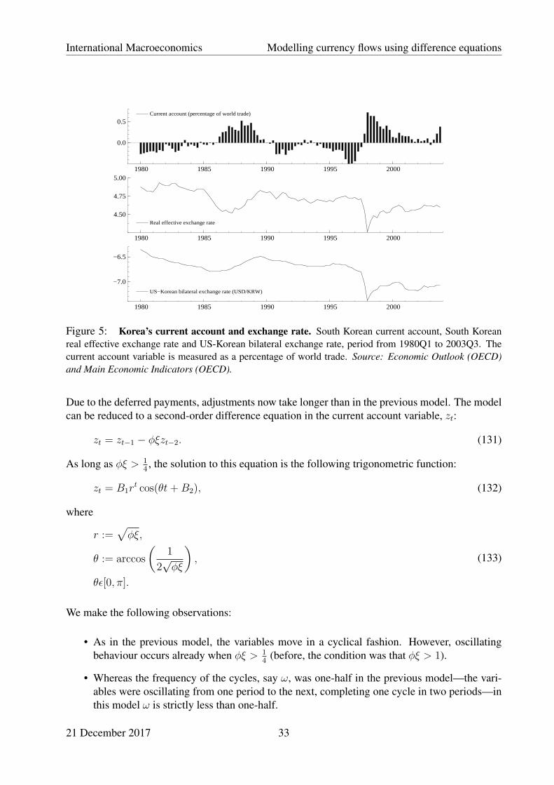
Figure 5: Korea’s current account and exchange rate. South Korean current account, South Koreanreal effective exchange rate and US-Korean bilateral exchange rate, period from 1980Q1 to 2003Q3. Thecurrent account variable is measured as a percentage of world trade. Source: Economic Outlook (OECD)and Main Economic Indicators (OECD).

Due to the deferred payments, adjustments now take longer than in the previous model. The modelcan be reduced to a second-order difference equation in the current account variable, zt:

zt = zt−1 − φξzt−2. (131)

As long as φξ > 14, the solution to this equation is the following trigonometric function:

zt = B1rt cos(θt+B2), (132)

where

r :=√φξ,

θ := arccos

(1

2√φξ

),

θε[0, π].

(133)

We make the following observations:

• As in the previous model, the variables move in a cyclical fashion. However, oscillatingbehaviour occurs already when φξ > 1

4(before, the condition was that φξ > 1).

• Whereas the frequency of the cycles, say ω, was one-half in the previous model—the vari-ables were oscillating from one period to the next, completing one cycle in two periods—inthis model ω is strictly less than one-half.

21 December 2017 33


1960 1965 1970 1975 1980 1985 1990 1995 2000

0.2

0.4

0.6

0.8

1.0

Japan Industrial countries All countries

Figure 6: Japan’s share of world reserves. Japan’s share of total reserves of all countries, plottedalongside the industrial countries’ share of worldwide reserves (monthly data, excluding gold reserves).Source: International Financial Statistics (IMF).

• The present model becomes unstable as soon as φξ > 1. In the previous model, the corres-ponding condition was that product of the parameters had to be greater than two, φξ > 2. Inother words, balance of payments and exchange rate fluctuations are potentially less stablewhen countries borrow from, and lend to, each other. With international borrowing and lend-ing, exchange rate adjustment is slower, implying that balance of payments imbalances cangrow larger.

• The correlation between the current account and the exchange rate is still positive; however,the exchange rate now lags the movements of the current account.

Benchmark model Model with debt

Oscillating behaviour φξ > 1 φξ > 14

Frequency of cycles ω = 12

ω < 12

Explosive behaviour φξ > 2 φξ > 1

Correlation between z and s Corr(zt, st) = +1 Corr(zt, st+1) = +1

since z1 = 1ξst since z1 = 1

ξst+1

Remarks:

• The period of the cycles in equation (132), p is:

p :=2π

θ. (134)

21 December 2017 34


• The frequency of the cycles in equation (132), ω, is:

ω :=1

p=

θ

2π. (135)

• Since for there to be cycles in zt, 14< φξ <∞, we know that 0 < θ < π. From there we get

the result regarding the frequency of the cycles:

0 < ω <1

2. (136)

21 December 2017 35

International Macroeconomics First-order ordinary differential equations

Part IV

Differential equations

4 Introduction to differential equations

Instead of using difference equations, it is sometimes more convenient to study economic modelsin continuous time using differential equations.

Definition:

• A differential equation is a mathematical equation for an unknown function of one or severalvariables that relates the values of the function itself and of its derivatives of various orders.

5 First-order ordinary differential equations

We denote the first and second derivative of a variable x with respect to time t as follows:

x :=dx

dt, x :=

d2x

dt2. (137)

What is a differential equation?

• In a differential equation, the unknown is a function, not a number.

• The equation includes one or more derivatives of the function.

The highest derivative of the function included in a differential equation is called its order.

Further, we distinguish ordinary and partial differential equations:

• An ordinary differential equation is one for which the unknown is a function of only onevariable. In our case, that variable will be time.

• Partial differential equations are equations where the unknown is a function of two or morevariables, and one or more of the partial derivatives of the function are included.

21 December 2017 36


5.1 Deriving the solution to a differential equation

Consider the first-order differential equation:

x(t) = ax(t) + b(t), (138)

The function b(t) is called ”forcing function”.

We can derive a solution as follows:

x(t)− ax(t) = b(t) (139)⇔ x(t)e−at − ax(t)e−at = b(t)e−at (140)

⇔ d

dt

[x(t)e−at

]= b(t)e−at. (141)

Note that the term e−at is called the ”integrating factor”. For t2 > t1, we obtain:

x(t2)e−at2 − x(t1)e−at1 =

∫ t2

t1

b(u)e−audu (142)

⇔ x(t2) = x(t1)ea(t2−t1) +

∫ t2

t1

b(u)e−a(u−t2)du (143)

⇔ x(t1) = x(t2)e−a(t2−t1) −∫ t2

t1

b(u)e−a(u−t1)du. (144)

(145)

Case where a < 0. In this case, as t1 → −∞:

x(t2)→∫ t2

−∞b(u)ea(t2−u)du (146)

or x(t)→∫ t

−∞b(u)ea(t−u)du. (147)

Case where a > 0. In this case, as t2 →∞:

x(t1)→ −∫ ∞t1

b(u)e−a(u−t1)du (148)

or x(t)→ −∫ ∞t

b(u)e−a(u−t)du. (149)

5.2 Applications

5.2.1 Inflation

Suppose that inflation increases whenever money growth falls short of current inflation:

π(t) = a (π(t)− µ(t)) , (150)

21 December 2017 37


where

π(t) = inflation,µ(t) = money growth,a > 0.

(151)

We can solve for π(t):

π(t) = aπ(t) + b(t), (152)

where

b(t) = −aµ(t). (153)

Then current inflation is determined by future money growth:

π(t) = −∫ ∞t

b(u)e−a(u−t)du

= a

∫ ∞t

µ(u)e−a(u−t)du.

(154)

5.2.2 Price of dividend-paying asset

Consider the following condition which equalizes the returns on an interest-bearing and a dividend-paying asset:

R =π(t)

q(t)+q(t)

q(t)(155)

⇔ q(t) = Rq(t)− π(t), (156)

where

R = interest rate (constant),q(t) = price of dividend-paying asset,π(t) = dividend.

(157)

The condition implies that the current price of the dividend-paying asset depends on the presentdiscounted value of all future dividends:

q(t) =

∫ ∞t

π(u)e−R(u−t)du. (158)

5.2.3 Monetary model of exchange rate

Consider a continuous-time version of the monetary model of exchange rate determination:

m(t)− p(t) = ay(t)− bR(t), (159)q(t) = p(t)− p∗(t) + s(t), (160)R(t) = R∗(t)− s(t). (161)

21 December 2017 38

International Macroeconomics Currency crises

The model can be rewritten in terms of an ordinary differential equation of the nominal exchangerate variable (for simplicity without the time argument):

s = R∗ −R

=1

b[(m−m∗)− (p− p∗)− a(y − y∗)]

=1

b[(m−m∗)− (q − s)− a(y − y∗)]

=1

bs+

1

b[(m−m∗)− q − a(y − y∗)] .

(162)

Solving this differential equation, we see that the current exchange rate is forward-looking anddepends on its future economic fundamentals:

s(t) =1

b

∫ ∞t

[−(m−m∗) + q + a(y − y∗)] e−1b(u−t)du. (163)

6 Currency crises

6.1 Domestic credit and reserves

Balance sheet of a central bank:

Assets Liablities

Bonds (D) Currency in circulationOfficial reserves (RS) Bank deposits

M = Currency + Bank deposits= RS +D

=RS +D

D×D

= eρD,

where

RS = official reserves,D = domestic credit,ρ = index of official reserves (≥ 0).

In logarithms:

m = ρ+ d.

The central bank creates money:

21 December 2017 39


• by buying domestic bonds (d ↑),

• by buying foreign reserves (ρ ↑).

The monetary model can therefore be modified as follows:

s = −(d− d∗)− (ρ− ρ∗) + a(y − y∗)− b(R−R∗) + q.

• Given the levels of the other variables, an increase in the domestic credit (purchase of do-mestic bonds) as well as an increase in reserves (purchase of foreign currency and bonds)induce a depreciation of the domestic currency (s ↓).

• However, it is also for instance possible to neutralize a domestic credit expansion by runningdown foreign reserves, keeping the exchange rate constant.

The previous equation may also be written in terms of percentage changes:

∆s = −(∆d−∆d∗)− (∆ρ−∆ρ∗) + a(∆y −∆y∗)− b(∆R−∆R∗) + ∆q,

where ∆ is the difference operator (that is, ∆x = xt−xt−1), or in terms of instantaneous percentagechanges (derivatives of the logarithms with respect to time):

s = −(d− d∗)− (ρ− ρ∗) + a(y − y∗)− b(R− R∗) + q.

6.2 A model of currency crises

The model we discuss is a simplified version of Flood and Garber (1984). See also Mark (2001,chapter 11.1).

From the definition of the real exchange rate, it follows that the nominal exchange rate is determ-ined as follows:

s(t) = −p(t) + p∗(t) + q(t). (164)

For simplicity, we assume that p∗(t) = 0. Another assumption, which we will relax later onhowever, is that purchasing power parity holds so that q(t) = 0.

The money market is given by the following equation:

m(t)− p(t) = ay(t)− bR(t), (165)

where national income, y(t), is set to zero for simplicity.

Finally, we assume that uncovered interest parity holds:

R(t) = R(t)∗ − s(t). (166)

We assume that R∗(t) = 0, again to make things simple.

21 December 2017 40


To sum up, the model consists of three simplified equations:

s(t) = −p(t), (167)m(t)− p(t) = −bR(t), (168)R(t) = −s(t). (169)

In addition, we assume that the domestic credit component of the national money supply grows atrate µ:

m(t) = ρ(t) + d(t), (170)d(t) = d(0) + µt. (171)

6.2.1 Exchange rate dynamics before and after the crisis

Using the first three equations of the model, we can derive a first-order differential equation in s(t):

bs(t) = s(t) +m(t) (172)

⇔ s(t) =1

bs(t) +

1

bm(t). (173)

The solution to this differential equation is:

s(t) = −∫ ∞t

1

bm(t)e−

1b(u−t)du. (174)

This integral may be further simplified using integration by parts. Note that integration by parts isbased on the following equation:∫ b

a

f(x)g′(x)dx =∣∣∣baf(x)g(x)−

∫ b

a

f ′(x)g(x)dx. (175)

In the case where f(x) = x and g′(x) = ex for instance, which is similar to ours, we obtain:∫ b

a

xexdx =∣∣∣baxex −

∫ b

a

exdx. (176)

As regards equation (174), we have to distinguish two cases:

• the time before the attack when m(t) = m(0) = d(0) + ρ(0),

• the time after the attack when m(t) = d(0) + µt.

In the first case, the exchange rate is constant:

s(t) = −∫ ∞t

1

bm(0)e−

1b(u−t)du. (177)

21 December 2017 41


f(u) = −1

bm(0), g′(u) = e−

1b(u−t), (178)

f ′(u) = 0, g(u) = −be−1b(u−t). (179)

s(t) =

∣∣∣∣∣∞

t

−1

bm(0)×

(−be−

1b(u−t)

)= −m(0)

= −d(0)− ρ(0).

(180)

This is, of course, the expected result from equation (172) when the exchange rate is fixed.

In the second case, after the exchange rate has started floating, the constant expansion of thedomestic credit leads to a continued depreciation:

s(t) = −∫ ∞t

1

b(d(0) + µu)e−

1b(u−t)du. (181)

f(u) = −1

b(d(0) + µu), g′(u) = e−

1b(u−t), (182)

f ′(u) = −1

bµ, g(u) = −be−

1b(u−t). (183)

s(t) =

∣∣∣∣∣∞

t

−1

b(d(0) + µu)×

(−be−

1b(u−t)

)−∫ ∞t

−1

bµ×

(−be−

1b(u−t)

)du

= −d(0)− µt− µb.(184)

6.2.2 Exhaustion of reserves in the absence of an attack

Time evolution of reserves:

ρ(t) = m(t)− d(t)

= m(0)− (d(0) + µt)

= ρ(0)− µt.(185)

Time of exhaustion of reserves:

ρ(0)− µtT = 0 (186)

⇔ tT =1

µρ(0). (187)

21 December 2017 42


6.2.3 Anticipated speculative attack

Time of speculative attack:

s(tA) = s(tA) (188)⇔ −d(0)− ρ(0) = −d(0)− µtA − µb (189)

⇔ tA =1

µρ(0)− b = tT − b. (190)

Reserves at the time of the speculative attack:

ρ(tA) = ρ(0)− µtA = ρ(0)− µ(

1

µρ(0)− b

)= µb > 0. (191)

Intuition:

• At the time of the attack, tA, people change abruptly their expectations regarding the depre-ciation of the exchange rate:

s(t) = 0 → s(t) < 0. (192)

• Uncovered interest parity implies a discrete rise in the interest rate and thus an immediatefall of the money demand:

R ↑ . (193)

• A sudden rise in prices (p(t) ↑) would help to restore equilibrium in the money market butwould imply a discrete downward jump of the exchange rate (s(t) ↓), which is not possiblesince speculators could make a riskless profit by selling the currency an instant before andbuying it an instant after the attack.

• The sudden fall in the money demand therefore has to be neutralized by a discrete reductionof the nominal money supply, m(t); that is, the central bank is forced to sell its remainingreserves in one final transaction:

ρ(t) ↓, m(t) ↓ . (194)

6.2.4 Fundamental causes of currency crises

In the model, we can distinguish between the short-term and the long-term causes of a currencycrisis:

• In the short term, a speculative attack on the domestic currency occurs because of the suddenchange in exchange rate expectations which force the central bank to sell all its remainingreserves at once.

21 December 2017 43


• The long-term cause of the crisis lies in the continuous expansion of the domestic credit, d(t),which oblige the central bank to run down its reserves to keep the money supply constant.

However, whereas the short-term cause of the speculative attack is a central feature of the model,the long-term cause is not; domestic credit expansion merely represents an example of how acurrency crisis can come about in the long run.

To see why, let us look once more at how changes in the nominal exchange rate come about (leavingaside the time argument of the functions for simplicity):

s = −p+ p∗ + q

= −(m− m∗) + a(y − y∗)− b(R− R∗)− c+ ˙q

= −(ρ− ρ∗)− (d− d∗) + a(y − y∗)− b(R− R∗) + z + k + r + ˙q,

(195)

where

c = payments (”cash flow”) balance(determining demand and supply in foreign exchange market),

z = current account,k = capital flow balance,r = changes in official reserves,q = residual exchange rate determinants

(neither value nor demand differences).

(196)

• Note that we have made use here of the balance of payments identity, z(t) + k(t) + c(t) +r(t) = 0.

• Remember also that acquisitions of foreign assets enter the financial account of the balanceof payments as debit items with a negative sign; for instance, all of the following transactionstake a negative sign:

– the acquisition of foreign capital by domestic residents and the sale of domestic capitalby foreigners (k(t) < 0, ”capital outflows”),

– money inflows (c < 0) and

– purchases of foreign reserves by the central bank (r < 0).

In practice, there are two important long-term causes of currency crises:

Domestic credit expansion

• Continued domestic credit expansion (d(t) > 0) leads to an increase in the domestic moneysupply.

• To avoid excessive growth of the money supply, the central bank must sell reserves (ρ(t) <0, r(t) > 0).

21 December 2017 44

International Macroeconomics Systems of differential equations

• Ultimately, the selling of foreign reserves will result in a speculative attack and a collapse ofthe exchange rate.

• The country could avoid a currency crisis by limiting the growth of its domestic credit.

Money outflows

• A persistent current account deficit or continued capital outflows (z(t) < 0, k(t) < 0) leadto large payments to foreigners (c(t) > 0), which drive up the demand for foreign currenciesat the expense of the domestic currency.

• To stabilize the exchange rate, the central bank needs to sell its reserves (ρ(t) < 0, r(t) > 0).

• Ultimately, the selling of foreign reserves will result in a speculative attack and a collapse ofthe exchange rate.

• Note that in this case, the depletion of reserves is not caused by growing domestic credit.Reducing domestic credit (d(t) < 0) will not be a useful remedy to avoid a currency crisissince it is likely to produce a recession. (This is a lesson that was learned during the currencycrises of the 1990s, particularly the Asian crisis of 1997–1998.)

• Instead it is important to stabilize the current account (for instance through a controlleddepreciation, a so-called crawling peg) and to restrict capital outflows (for instance throughcapital controls).

7 Systems of differential equations

7.1 Uncoupling of differential equations

Consider the system of differential equations:

x(t) = A x(t) + b(t) .n× 1 n× n n× 1 n× 1

(197)

Note that the system contains n interdependent equations so that our previous method of analysingdifferential equations does not apply.

However, suppose that A is diagonalizable, that is:

A = PΛP−1 (198)

where

P = (p1,p2, . . . ,pn)n×n,

Λ = diag(λ1, λ2, . . . , λn)n×n,

pi = ith eigenvector of A,λi = ith eigenvalue of A.

(199)

21 December 2017 45


We may now transform the original system of differential equations in (197) into a set of n inde-pendent (orthogonal) equations as follows:

x(t) = Ax(t) + b(t) (200)⇔ x(t) = PΛP−1x(t) + b(t) (201)⇔ P−1x(t) = ΛP−1x(t) + P−1b(t) (202)⇔ x∗(t) = Λx∗(t) + b∗(t) (203)

Our previous method of solving differential equations may now be applied to each of the n inde-pendent equations. At any time, x(t) and b(t) may be recovered as follows:

x(t) = Px∗(t), b(t) = Pb∗(t). (204)

7.2 Dornbusch model

The Dornbusch model is presented in many textbooks, for example in Heijdra and van der Ploeg(2002) and Obstfeld and Rogoff (1996).

7.2.1 The model’s equations

The Dornbusch model is based on the following relations:

y = −cR + dG− e(s+ p− p∗), (205)m− p = ay − bR, (206)R = R∗ − s, (207)p = f(y − y). (208)

• Endogenous variables: y, R, s, p.

• Exogenous variables: m, G, y, p∗, R∗.

• Parameters (all positive): a, b, c, d, e, f.

7.2.2 Long-run characteristics

We may derive the long-run characteristics by setting s = 0 and p = 0:

• Monetary neutrality: p = m in the long run, and no effect of m on y or R.

• Unique equilibrium real exchange rate:

q = s+ p− p∗

=1

e(−y − cR∗ + dG) .

(209)

Note that the equilibrium real exchange rate is not affected by monetary policy but that it can beaffected by fiscal policy.

21 December 2017 46


7.2.3 Short-run dynamics

To study the short-run dynamics implied by the model, let us reduce the model to a system of twodifferential equations in s and p. Note first that for given values of the nominal exchange rate andthe domestic price level, the domestic output and interest rate can be written as:

y =c(m− p) + bdG− be(s+ p− p∗)

b+ ac,

R =−(m− p) + adG− ae(s+ p− p∗)

b+ ac.

(210)

s = R∗ −R

= R∗ +(m− p)− adG+ ae(s+ p− p∗)

b+ ac,

p = f(y − y)

= fc(m− p) + bdG− be(s+ p− p∗)

b+ ac− fy.

(211)

[s

p

]=

[aeb+ac

ae−1b+ac

− befb+ac

− cf+befb+ac

][s

p

]+

[1

b+ac−adb+ac

0 −aeb+ac

1

cfb+ac

bdfb+ac

−f befb+ac

0

]mGyp∗

R∗

. (212)

We shall assume that ae < 1.

In a diagram with p on the horizontal and s on the vertical axis, the s = 0 curve is upward-slopingsince s = 0 implies:

s =1− aeae

p+− 1

aem+

d

eG+ p∗ − b+ ac

aeR∗. (213)

On the other hand, the p = 0 curve is downward-sloping since p = 0 implies:

s = −c+ be

bep+

c

bem+

d

eG− b+ ac

bey + p∗. (214)

We may now analyse the model in a phase diagram with s on the vertical and p on the horizontalaxis.

In doing so, we assume that:

• the exchange rate, s, is a jump variable that moves instantaneously towards any level requiredto achieve equilibrium in the long run and that

21 December 2017 47

International Macroeconomics Laplace transforms

• the price level, p, is a crawl variable that moves continuously without abrupt jumps.

We are interested to answer the following questions:

• Is the system saddle-path stable?

(The condition for the model to be saddle-path stable is that |A| < 0 and is here fulfilled.)

• How is the adjustment towards the equilibrium?

• How does the equilibrium and the adjustment towards the equilibrium change if there is achange in one or several of the exogenous variables.

8 Laplace transforms

The main purpose of Laplace transforms is the solution of differential equations and systems ofsuch equations, as well as corresponding initial value problems.

Useful introductions to Laplace transforms can be found in ? and Kreyszig (1999).

8.1 Definition of Laplace transforms

The Laplace F (s) = L{f(t)} of a function f(t) is defined by:

F (s) = L{f(t)} =

∫ ∞0

f(t)e−stdt. (215)

It is important to note that the original function f depends on t and that its transform, the newfunction F , depends on s.

The original function f(t) is called the inverse transform, or inverse, of F (s) and we write:

f(t) = L−1(F ). (216)

To avoid confusion, it is useful to denote original functions by lowercase letters and their trans-forms by the same letters in capitals:

f(t)→ F (s), g(t)→ G(s), etc. (217)

21 December 2017 48


8.2 Standard Laplace transforms

f(t) F(s) = L{f(t)}

1 1s

t 1s2

t2 2!s3

tn n!sn+1

tn−1

(n−1)!1sn

eat 1s−a

f(t) F(s) = L{f(t)}

sin(at) as2+a2

cos(at) ss2+a2

sinh(at) as2−a2

cosh(at) ss2−a2

u(t− c) e−cs

s

δ(t− a) e−as

Of course, these tables can also be used to find inverse transforms.

8.3 Properties of Laplace transforms

8.3.1 Linearity of the Laplace transform

The Laplace transform is a linear transform:

L{af(t) + bg(t)} = aL{f(t)}+ bL{g(t)}. (218)

8.3.2 First shift theorem

The first shift theorem states that if L{f(t)} = F (s) then:

L{e−atf(t)} = F (s+ a). (219)

8.3.3 Multiplying and dividing by t

If L{f(t)} = F (s), then

L{tf(t)} = −F ′(s). (220)

If L{f(t)} = F (s), then

L

{f(t)

t

}=

∫ ∞s

F (σ)dσ, (221)

provided limt→0

{f(t)t

}exists.

21 December 2017 49


8.3.4 Laplace transforms of the derivatives of f(t)

The Laplace transforms of the derivatives of f(t) are as follows:

L{f ′(t)} = sL{f(t)} − f(0),

L{f ′′(t)} = s2L{f(t)} − sf(0)− f ′(0),

L{f ′′′(t)} = s3L{f(t)} − s2f(0)− sf ′(0)− f ′′(0).

(222)

It is convenient to adopt a more compact notation here, letting x := f(t) and x := L{x}:

L{x} = x,

L{x} = sx− x(0),

L{x} = s2x− sx(0)− x(0),

L{...x} = s3x− s2x(0)− sx(0)− x(0),

L{....x } = s4x− s3x(0)− s2x(0)− sx(0)− ...x(0).

(223)

8.3.5 Second shift theorem

The second shift theorem states that if L{f(t)} = F (s) then:

L{u(t− c)f(t− c)} = e−csF (s), (224)L−1{e−csF (s)} = u(t− c)f(t− c). (225)

This theorem turns out to be useful in finding inverse transforms.

8.4 Solution of differential equations

8.4.1 Solving differential equations using Laplace transforms

Many differential equations can be solved using Laplace transforms as follows:

• Rewrite the differential equation in terms of Laplace transforms.

• Insert the given initial conditions.

• Rearrange the equation algebraically to give the transform of the solution.

• Express the transform in standard form by partial fractions.

• Determine the inverse transforms to obtain the particular solution.

21 December 2017 50


8.4.2 First-order differential equations

First-order differential equation:

x(t) = 2x(t) = 4, (226)

where

x(0) = 1. (227)

Solution:

• Laplace transforms:

(sx− x(0))− 2x =4

s. (228)

• Initial condition:

sx− 1− 2x =4

s. (229)

• Solve for x:

x =s+ 4

s(s− 2). (230)

• Partial fractions:

x =3

s− 2− 2

s. (231)

• Inverse transforms:

x(t) = 3e2t − 2. (232)

8.4.3 Second-order differential equations

Second-order differential equation:

x(t)− 3x(t) + 2x(t) = 2e3t, (233)

where

x(0) = 5,

x(0) = 7.(234)

Solution:

21 December 2017 51


• Laplace transforms:(s2x− sx(0)− x(0)

)− 3(sx− x(0)) + 2x =

2

s− 3. (235)

• Initial conditions:(s2x− 5s− 7

)− 3(sx− 5) + 2x =

2

s− 3. (236)

• Solve for x:

x =5s2 − 23s+ 26

(s− 1)(s− 2)(s− 3)(237)


x =4

s− 1+

1

s− 3. (238)


x(t) = 4et + e3t. (239)

8.4.4 Systems of differential equations

Systems of differential equations:

y(t)− x(t) = et, (240)x(t) + y(t) = e−t, (241)

where

x(0) = y(0) = 0. (242)

Solution:


(sy − y(0))− x =1

s− 1, (243)

(sx− x(0)) + y =1

s+ 1. (244)

• Initial conditions:

sy − x =1

s− 1, (245)

sx+ y =1

s+ 1. (246)

21 December 2017 52

International Macroeconomics The model of section 6.2 revisited

• Solve for x:

x =s2 − 2s− 1

(s− 1)(s+ 1)(s2 + 1). (247)


x =1

2

1

s− 1− 1

2

1

s+ 1+

s+ 1

s2 + 1. (248)


x(t) = −1

2et − 1

2e−t + cos t+ sin t. (249)

• Obtain y(t) from y(t) = −x(t) + e−t:

y(t) =1

2et +

1

2e−t − cos t+ sin t. (250)

9 Solving the model of section 6.2 using Laplace transforms

Let us use the Laplace transform method to solve once again the currency crisis model of sec-tion 6.2.

Recall the differential equation (172), which describes the nominal exchange rate’s dynamics be-fore and after the attack:

s(t) =1

bs(t) +

1

bm(t). (251)

Let us consider the case where the exchange rate has already started to float after being attacked,so that m(t) = d(0) + µt. To avoid confusion with the parameter s of the Laplace transform, weuse the function x(t) rather than s(t) to denote the exchange rate. Then we have:

x(t) =1

bx(t) +

1

b(d(0) + µt). (252)

Here is how we can solve the differential equation for s(t) using Laplace transforms:

sx− x(0) =1

bx+

1

b

(d(0)

s+µ

s2

)(253)

⇔ x =bx(0)s2 + d(0)s+ µ

s2(sb− 1). (254)

Now we take partial fractions:

x =−d(0)− µb

s− µ

s2+x(0) + d(0) + µb

s− 1b

. (255)

Taking the inverse Laplace transforms of the resulting terms, we obtain:

x(t) = −d(0)− µb− µt+ (x(0) + d(0) + µb) e1bt. (256)

We see that there are infinitely many solutions, depending on the choice of the initial condition.

21 December 2017 53

International Macroeconomics A model of currency flows in continuous time

• If we choose x(0) = −d(0)−µb as the initial condition, we obtain the linear solution alreadyencountered in equation (184).

• However, with any other initial condition, the exchange rate will diverge exponentially fromthe linear trend given by −d(0)− µb− µt.

10 A model of currency flows in continuous time

10.1 The model’s equations

We now consider model of currency flows and exchange rate movements in continuous time. Themodel consists of the following equations:

s(t) = −ξc(t), (257)q(t) = s(t), (258)z(t) = −φq(t), (259)c(t) = −z(t). (260)

10.2 Solving the model as a system of differential equations

Let us write the model a little more compactly:

q(t) = ξz(t), (261)z(t) = −φq(t). (262)

Solution using Laplace transforms:


(sq − q(0)) = ξz,

(sz − z(0)) = −φq.(263)

• Solve for z:

z =sz(0)− φq(0)

s2 + ξφ. (264)


z(t) = z(0) cos(√

ξφ t)−φq(0) sin

(√ξφ t)

√ξφ

(265)

• Obtain q(t) from z(t) = −φq(t):

q(t) =1

φz(t)

=1

φ

[−√ξφ z(0) sin

(√ξφ t)− φq(0) cos

(√ξφ t)] (266)

21 December 2017 54

International Macroeconomics A model of currency flows in continuous time

10.3 Solving the model as a second-order differential equation

Note that the model can also be expressed in terms of a second-order differential equation in z(t):

z(t) + ξφz(t) = 0. (267)

Solving this equation should obviously lead to the same final solution:

• Laplace transforms:((s2z − sz(0)− z(0)

)+ ξφz = 0. (268)

• Solve for z:

z =sz(0) + z(0)

s2 + ξφ. (269)


z(t) = z(0) cos(√

ξφ t)

+z(0) sin

(√ξφ t)

√ξφ

(270)

• Obtain q(t) from z(t) = −φq(t):

q(t) =1

φz(t)

=1

φ

[−√ξφ z(0) sin

(√ξφ t)

+ z(0) cos(√

ξφ t)] (271)

In this model,

• the cyclical fluctuations come about since current account imbalances immediately produceoffsetting payment flows,

• which push the exchange rate either up or down (depending on whether the current accountis in surplus or in deficit).

Any current account imbalance thus carries with it the seed of its own reversal.

Now compare the model’s prediction with the swings in Japan’s and Germany’s current accountand exchange rate data plotted in figures 7 and 8.

21 December 2017 55

International Macroeconomics Intertemporal approach to the current account

1970 1975 1980 1985 1990 1995 2000

−2.5

0.0

2.5

5.0

7.5

10.0

12.5

15.0

17.5

Current account

3.4

3.6

3.8

4.0

4.2

4.4

4.6Nominal effective exchange rate Nominal effective exchange rate (counterfactual)

Figure 7: Japanese current account and counterfactual exchange rate. Japanese current account (leftscale, in trillions of yen, transformed from biannual to quarterly frequency using a natural cubic splinesmooth) and nominal effective exchange rate (right scale, in logarithms), period from 1968Q1 to 1999Q4.The exchange rate is plotted along with counterfactual estimates during the periods 1980Q1–1981Q4 and1984Q2–1986Q2 when measures to liberalize Japan’s capital account took effect, inducing capital inflows inthe early 1980s and capital outflows in the mid-1980s. The counterfactual series was calculated by removingthe exchange rate observations during the years of increased capital in- or outflows and filling the missingvalues with the estimates from a natural cubic spline smooth based on all remaining observations. Source:Economic Outlook (OECD), IFS (IMF), own calculations.

Part V

Intertemporal optimization

11 Methods of intertemporal optimization

• Ordinary maximization

• Calculus of variations

• Optimal control

• Dynamic programming

12 Intertemporal approach to the current account

See Obstfeld and Rogoff (1995, 1996).

21 December 2017 56

International Macroeconomics Intertemporal approach to the current account

−5

0

5

10

15

20

25

4.15

4.20

4.25

4.30

4.35

4.40

4.45

4.50

1980 1985 1990

Current account Nominal effective exchange rate

Figure 8: German current account and nominal exchange rate in the 1980s. German current account(left scale, in German mark) and nominal effective exchange rate (right scale, in logarithms), period from1977Q1 to 1990Q4. Source: International Financial Statistics (IMF).

12.1 Current account

Current account balance of a country:

• exports minus imports of goods and services (elasticities approach), rents on labour andcapital, unilateral transfers;

• increase in residents’ claims on foreign incomes or outputs less increase in similar foreign-owned claims on home income or output;

• national saving less domestic investment (absorption approach, intertemporal approach).

The intertemporal approach views the current account balance as the outcome of forward-lookingdynamic saving and investment decisions.

12.2 A one-good model with representative national residents

Consider a small open economy that produces and consumes a single composite good and tradesfreely with the rest of the world.

The current account, CAt, is equal to the accumulation of net foreign assets and to the saving-investment balance:

CAt = Bt+1 −Bt = rtBt + Yt − Ct −Gt − It, (272)

21 December 2017 57

International Macroeconomics Ordinary maximization by taking derivatives

where

Bt+1 := stock of net foreign assets at the end of period t,rt := interest rate,Yt := domestic output,Ct := private consumption,Gt := government consumption,It := net investment.

(273)

13 Ordinary maximization by taking derivatives

13.1 Two-period model of international borrowing and lending

Utility:

U1 = u(C1) + βu(C2). (274)

Intertemporal budget constraint:

Y1 + (1 + r)B1 = C1 +B2, (275)Y2 + (1 + r)B2 = C2 +B3. (276)

Current account:

CA1 = S1 = B2 −B1 = Y1 + rB1 − C1, (277)CA2 = S2 = B3 −B2 = Y2 + rB2 − C2. (278)

Combining the intertemporal budget constraints yields:

Y1 +1

1 + rY2 + (1 + r)B1 = C1 +

1

1 + rC2 +

1

1 + rB3 (279)

⇔ C2 = (1 + r)Y1 + Y2 + (1 + r)2B1 − (1 + r)C1 −B3 (280)

⇔ C1 = Y1 +1

1 + rY2 + (1 + r)B1 −

1

1 + rC2 −

1

1 + rB3. (281)

Maximization problem:

maxC1

= u(C1) + βu((1 + r)Y1 + Y2 + (1 + r)2B1 − (1 + r)C1 −B3) (282)

First-order condition:

u′(C1)− β(1 + r)u′(C2) = 0 ⇔ βu′(C2)

u′(C1)=

1

1 + r. (283)

21 December 2017 58



maxC2

= u

(Y1 +

1

1 + rY2 + (1 + r)B1 −

1

1 + rC2 −

1

1 + rB3

)+ βu(C2) (284)


− 1

1 + ru′(C1)− βu′(C2) = 0 ⇔ βu′(C2)

u′(C1)=

1

1 + r. (285)


maxB2

= u(Y1 + (1 + r)B1 −B2) + βu(Y2 + (1 + r)B2 −B3) (286)


−u′(C1) + β(1 + r)u′(C2) = 0 ⇔ βu′(C2)

u′(C1)=

1

1 + r. (287)

Let B1 = B3 = 0. Let u(·) = log(·). Then:

C1 =1

β(1 + r)C2 =

1

1 + β

(Y1 +

1

1 + rY2

), (288)

C2 =β

1 + β((1 + r)Y1 + Y2) . (289)

Current accounts:

CA1 = B2 −B1 =β

1 + βY1 −

1

(1 + β)(1 + r)Y2, (290)

CA2 = B3 −B2 = − β

1 + βY1 +

1

(1 + β)(1 + r)Y2. (291)

13.2 Digression on utility functions

13.2.1 Logarithmic utility.

Logarithmic utility is given by:

u(C) = log(C),

u′(C) =1

C> 0,

u′′(C) = − 1

C2< 0,

γ(C) = −u′′(C)

u′(C)=

1

C,

γ(C) = −du′(C)u′(C)

dCC

= −Cu′′(C)

u′(C)= 1,

σ(C) =1

γ(C)= −

dCC

du′(C)u′(C)

= − u′(C)

Cu′′(C)= 1,

(292)

21 December 2017 59


where

• γ(C) is the absolute risk aversion, or the reciprocal of the so-called risk tolerance,

• γ(C) is the relative risk aversion, or consumption elasticity of marginal utility, and

• σ(C) is the elasticity of intertemporal substitution.

13.2.2 Isoelastic utility.

The class of period utility functions characterized by a constant elasticity of intertemporal substi-tution is:

u(C) =C1− 1

σ

1− 1σ

, σ > 0,

u′(C) = C−1σ > 0,

u′′(C) = − 1

σC−

1σ−1 < 0,

γ(C) = −u′′(C)

u′(C)=

1

σC,

γ(C) = −Cu′′(C)

u′(C)=

1

σ= γ = const.

σ(C) =1

γ(C)= σ = const.

(293)

For σ = 1, the isoelastic utility function is replaced by its limit, log(C).

13.2.3 Linear-quadratic utility.

Linear-quadratic utility is given by:

u(C) = −(b− C)2

2,

u′(C) = b− C, u′(C) ≥ 0 if C ≤ b,

u′′(C) = −1 < 0,

γ(C) = −u′′(C)

u′(C)=

1

b− C,

γ(C) = −Cu′′(C)

u′(C)=

C

b− C,

σ(C) =1

γ(C)=

b

C− 1.

(294)

21 December 2017 60


13.2.4 Exponential utility.

Exponential utility is given by:

u(C) = −be−Cb , b > 0,

u′(C) = e−Cb > 0,

u′′(C) = −1

be−

Cb < 0,

γ(C) = −u′′(C)

u′(C)=

1

b= const.,

γ(C) = −Cu′′(C)

u′(C)=C

b,

σ(C) =1

γ(C)=

b

C.

(295)

13.2.5 The HARA class of utility functions

A HARA utility function, u(C), is one whose absolute risk aversion is hyperbolic:

γ = −u′′(C)

u′(C)=

1

aC + b> 0, (296)

for some constants a and b. Since the inverse of absolute risk aversion is risk tolerance, a HARAutility function exhibits linear risk tolerance:

1

γ= − u

′(C)

u′′(C)= aC + b > 0. (297)

The relative risk aversion of a HARA utility function is given by:

γ(C) = −Cu′′(C)

u′(C)=

C

aC + b=

1

a− b

a2C + ab. (298)

For a utility function of the HARA class:

• risk tolerance (the reciprocal of absolute risk aversion) is a linearly increasing function of aand is constant if a = 0;

• relative risk aversion is rising with b and is constant if b = 0.

It can be shown that all the utility functions mentioned above belong to the HARA family:

Utility function a b

Logarithmic > 0 = 0Isoelastic > 0 = 0Linear-quadratic < 0 > 0Exponential = 0 > 0

21 December 2017 61


13.3 Two-period model with investment

Production function:

Y = F (K). (299)

As usual, F ′(K) > 0, F ′′(K) < 0 and F (0) = 0.

Utility:

U1 = u(C1) + βu(C2). (300)

Intertemporal budget constraint, where It = Kt+1 −Kt:

Y1 + (1 + r)B1 +K1 = C1 +B2 +K2, (301)Y2 + (1 + r)B2 +K2 = C2 +B3 +K3. (302)

Current account:

CA1 = S1 − I1 = B2 −B1 = Y1 + rB1 − C1 − I1, (303)CA2 = S2 − I2 = B3 −B2 = Y2 + rB2 − C2 − I2. (304)

Combining the intertemporal budget constraints yields:

Y1 +1

1 + rY2 + (1 + r)B1 +K1 = C1 +

1

1 + rC2 +

1

1 + rB3 +

1

1 + rK3 (305)

⇔ C2 = (1 + r)Y1 + Y2 + (1 + r)2B1 + (1 + r)K1 − (1 + r)C1 −B3 −K3 (306)

⇔ C1 = Y1 +1

1 + rY2 + (1 + r)B1 −

1

1 + rC2 −

1

1 + rB3 −

1

1 + rK3. (307)


maxB2,K2

= u(F (K1) + (1 + r)B1 +K1 −B2 −K2)

+ βu(F (K2) + (1 + r)B2 + K2 − B3 −K3) (308)

First-order conditions:

−u′(C1) + β(1 + r)u′(C2) = 0 ⇔ βu′(C2)

u′(C1)=

1

1 + r, (309)

−u′(C1) + β(1 + F ′(K2))u′(C2) = 0. ⇔ βu′(C2)

u′(C1)=

1

1 + F ′(K2). (310)

(311)

Therefore returns on capital and foreign assets must be equal:

F ′(K2) = r. (312)

Let B1 = B3 = 0. Let u(·) = log(·). Then:

C1 =1

β(1 + r)C2 =

1

1 + β

(Y1 +

1

1 + rY2

), (313)

C2 =β

1 + β((1 + r)Y1 + Y2) . (314)

21 December 2017 62


13.4 An infinite-horizon model

Utility at time t:

Ut =∞∑s=t

βs−tu(Cs). (315)

Intertemporal budget constraint:

AsF (Ks) + (1 + r)Bs +Ks = Cs +Bs+1 +Ks+1 +Gs (316)

The infinite-horizon budget constraint is:∞∑s=t

(1

1 + r

)s−tYs + (1 + r)Bt =

∞∑s=t

(1

1 + r

)s−t(Cs + Is +Gs). (317)

Here it is assumed that the transversality condition holds:

limT→∞

(1

1 + r

)TBt+T+1 = 0. (318)


maxBs+1,Ks+1

∞∑s=t

βs−tu[AsF (Ks) + (1 + r)Bs +Ks −Bs+1 −Ks+1 −Gs] (319)


−u′(Cs) + β(1 + r)u′(Cs+1) = 0 (320)

⇔ βu′(Cs+1)

u′(Cs)=

1

1 + r, (321)

−u′(Cs) + β(1 + As+1F′(Ks+1))u′(Cs+1) = 0 (322)

⇔ βu′(Cs+1)

u′(Cs)=

1

1 + As+1F ′(Ks+1). (323)

Therefore returns on capital and foreign assets must be equal:

As+1F′(Ks+1) = r. (324)

Note that when β = 1/(1 + r), optimal consumption is constant:

Ct =r

1 + r

[(1 + r)Bt +

∞∑s=t

(1

1 + r

)s−t(Ys −Gs − Is)

]. (325)

If the period utility function is isoelastic, the Euler equation (320) takes the form

Cs+1 = (1 + r)σβσCs. (326)

21 December 2017 63


We can use it to eliminate Ct+1, Ct+2, etc. from budget constraint (317). Under the assumption that(1 + r)σ−1βσ < 1, so that consumption grows a a net rate below r, the result is the consumptionfunction

Ct =(1 + r)Bt +

∑∞s=t

(1

1+r

)s−t(Ys − Is −Gs)∑∞

s=t[(1 + r)σ−1βσ]s−t. (327)

Defining θ ≡ 1− (1 + r)σβσ, we rewrite this as:

Ct =r + θ

1 + r

[(1 + r)Bt +

∞∑s=t

(1

1 + r

)s−t(Ys − Is −Gs)

]. (328)

Given r, consumption is a decreasing function of β.

13.5 Dynamics of the current account

See Obstfeld and Rogoff (1996, section 2.2).

For a constant interest rate r, define the permanent level of a variable X on date t by:

∞∑s=t

(1

1 + r

)s−tXt =

∞∑s=t

(1

1 + r

)s−tXs, (329)

so that

Xt =r

1 + r

∞∑s=t

(1

1 + r

)s−tXs. (330)

The permanent level of X , X , is its annuity value at the prevailing interest rate.

Using (325), we obtain:

CAt = Bt+1 −Bt

= Yt + rBt − Ct − It −Gt

= (Yt − Yt)− (It − It)− (Gt − Gt).

(331)

When β 6= 1/(1 + r) and utility is isoelastic,

CAt = (Yt − Yt)− (It − It)− (Gt − Gt)−θ

1 + rWt, (332)

where

Wt = (1 + r)Bt +∞∑s=t

(1

1 + r

)s−t(Ys − Is −Gs) (333)

and θ = 1− (1 + r)σβσ.

21 December 2017 64


13.6 A model with consumer durables

See Obstfeld and Rogoff (1996, section 2.4).

Let Cs be consumption of nondurables and Ds be the stock of durable goods the consumer ownsas date s ends. A stock of durables yields its owner a proportional service flow each period it isowned. Let p be the price of durable goods in terms of nondurable consumption (determined in theworld market).

Utility function

Ut =∞∑s=t

βs−t[γ logCs + (1− γ) logDs] (334)

Period-to-period budget constraint:

F (Ks) + (1 + rs)Bs +Ks + ps(1− δ)Ds−1 = Cs +Bs+1 +Ks+1 + psDs +Gs, (335)

where ps[Ds − (1− δ)Ds−1] is the cost of durable goods purchases in period s.


maxBs+1,Ks+1,Ds

∞∑s=t

βs−t[γ logCs + (1− γ) logDs], (336)

where Cs = F (Ks)− [Bs+1 − (1 + rs)Bs]− (Ks+1 −Ks)− ps[Ds − (1− δ)Ds−1]−Gs.


− 1

Cs+ β(1 + rs)

1

Cs+1

= 0, (337)

− 1

Cs+ β(1 + F ′(Ks+1)

1

Cs+1

= 0, (338)

1− γDs

− γpsCs

+βγps+1(1− δ)

Cs+1

= 0. (339)

Rewrite these equations:

rs = F ′(Ks+1), (340)Cs+1 = β(1 + rs)Cs, (341)(1− γ)CsγDs

= ps −1− δ

1 + rs+1

ps+1 ≡ ιs. (342)

Here, ι is the implicit date s rental price, or user cost, of the durable good, that is, the net expenseof buying the durable in one period, using it in the same period, and selling it in the next. Equa-tion (342) states that, at an optimum, the marginal rate of substitution of nondurables consumptionfor the services of durables equals the user cost of durables in terms of nondurables consumption.

21 December 2017 65


Intertemporal budget constraint (with constant r):

∞∑s=t

(1

1 + r

)s−t(Cs + ιsDs) =

(1 + r)Bt + (1 − δ)ptDt−1 +∞∑s=t

(1

1 + r

)s−t(Ys − Gs − Is). (343)

This constraint states that the present value of expenditures (the sum of nondurables purchases plusthe implicit rental cost of the durables held) equals initial financial assets (including durables) plusthe present value of net output.

Assuming that β = 1/(1 + r) (so that nondurables and durables consumption is constant):

Ct =γr

1 + r

[(1 + r)Bt + (1− δ)ptDt−1 +

∞∑s=t

(1

1 + r


](344)

Dt =(1− γ)r

ι(1 + r)

[(1 + r)Bt + (1− δ)ptDt−1 +

∞∑s=t

(1

1 + r


](345)

How do durables affect the current account? With p constant:

p =

(1 + r

1 + δ

)(1− γγ

)CsDs

, s ≥ t. (346)

Let Z = Y −G− I . Then:

CAt = Bt+1 −Bt = rBt + Zt −Ctγ− (1− γ)Ct

γ− p[Dt − (1− δ)Dt−1]

=

[Zt −

r

1 + r

∞∑s=t

(1

1 + r

)s−tZs

]

− 1− δ1 + r

pDt−1 +(1− γ)Ct

γ− pDt + (1− δ)pDt−1

= (Yt − Yt)− (It − It)− (Gt − Gt) + (ι− p)∆Dt.

(347)

13.7 Firms, the labour market and investment

See Obstfeld and Rogoff (1996, section 2.5.1).

The production function (homogeneous to degree one) is AF (K,L), where L is constant. We canthink of output as being produced by a single representative domestic firm that behaves compet-itively and is owned entirely by domestic residents. Vt is the date t price of a claim to the firm’sentire future profits (starting on date t + 1). Let xs+1 be the share of the domestic firm owned bythe representative consumer at the end of date s and ds the dividends the firm issues on date s.

21 December 2017 66


13.7.1 The consumer’s problem.

Utility function:

Ut =∞∑s=t

u(Cs). (348)

Period-to-period financial constraint:

Bs+1 −Bs + Vsxs+1 − Vs−1xs = rBs + dsxs + (Vs − Vs−1)xs + wsL− Cs −Gs. (349)


maxBs+1,xs+1

∞∑s=t

u[(1 + r)Bs −Bs+1 − Vs(xs+1 − xs) + dsxs + wsL−Gs]. (350)


u′(Cs) = (1 + r)βu′(Cs+1), (351)Vsu

′(Cs) = (Vs+1 + ds+1)βu′(Cs+1). (352)

From this, we see that returns on foreign bonds and shares must be equal:

1 + r =ds+1 + Vs+1

Vs(353)

A useful reformulation of the individual’s budget constraint uses the variable Qs+1, which is thevalue of the individual’s financial wealth at the end of period s:

Qs+1 = Bs+1 + Vsxs+1. (354)

The period-to-period financial constraint becomes:

Qs+1 −Qs = rQs + wsL− Cs −Gs, s = t+ 1, t+ 2, . . . , (355)Qt+1 = (1 + r)Bt + dtxt + Vtxt + wtL− Ct −Gt. (356)

By forward iteration, we obtain:

∞∑s=t

(1

1 + r

)s−tCs = (1 + r)Bt + dtxt + Vtxt +

∞∑s=t

(r

1 + r

)s−t(wsL−Gs). (357)

Here it is supposed that the following transversality condition holds:

limT→∞

(1

1 + r

)TQt+T+1 = 0. (358)

21 December 2017 67


13.7.2 The stock market value of the firm.

Note that equation (353) implies:

Vt =dt+1

1 + r+Vt + 1

1 + r

=∞∑t+1

(1

1 + r

)s−tds.

(359)

We rule out self-fulfilling speculative asset-price bubbles:

limT→∞

(1

1 + r

)TVt+T = 0. (360)

13.7.3 Firm behaviour.

The dividends a firm pays out in a period are its current profits less investment expenditure, that is,ds = Ys − wsLs − Is. The value of the firm can therefore be written as follows:

Vt =∞∑

s=t+1

(1

1 + r

)s−t[AsF (Ks, Ls)− wsLs − (Ks+1 −Ks)]. (361)

The firm maximizes the present value of current and future dividends, given Kt:

dt + Vt =∞∑s=t

(1

1 + r

)s−t[AsF (Ks, Ls)− wsLs − (Ks+1 −Ks)]. (362)

First-order conditions for capital and labour:

AsFK(Ks, Ls) = r, s > t, (363)AsFL(Ks, Ls) = ws, s ≥ t. (364)

Note that the consumer’s problem is the same is the same as in an economy without a firm, wherethe consumer is itself the producer. This is so since the Euler equation and budget constraints areidentical, provided the equilibrium conditions xs = 1 and Ls = L hold on all dates s. To see this,combine equations (361) and (351).

13.8 Investment when capital is costly to install: Tobin’s q

See Obstfeld and Rogoff (1996, section 2.5.2).

There are now quadratic installation costs for investment. The firm maximizes, for a given Kt:

dt + Vt =∞∑s=t

(1

1 + r

)s−t [AsF (Ks, Ls)−

χ

2

I2s

Ks

− wsLs − Is], (365)

21 December 2017 68


subject to

Ks+1 −Ks = Is. (366)

Lagrangian, to differentiate with respect to labour, investment and capital:

Lt =∞∑s=t

(1

1 + r

)s−t [AsF (Ks, Ls)−

χ

2

I2s

Ks

− wsLs − Is − qs(Ks+1 −Ks − Is)].

(367)


AsFL(Ks, Ls)− w = 0, (368)

−χIsKs

− 1 + qs = 0, (369)

−qs +As+1FK(Ks+1, Ls+1) + χ

2(Is+1/Ks+1)2 + qs+1

1 + r= 0. (370)

21 December 2017 69

International Macroeconomics Optimal control theory

Part VI

Dynamic optimization in continuous time

14 Optimal control theory

14.1 Deriving the fundamental results using an economic example

A firm wishes to maximize its total profits over some period of time starting at date t = 0 andending at date T :

W (k0,x) =

∫ T

0

u(k, x, t)dt

The variable kt is the capital stock at date t, the initial capital stock k0 is given to the firm. Thevariable xt is chosen by the firm at every instant. The function u(kt, xt, t) determines the rate atwhich profits are being earned at time t as a result of having capital k and taking decisions x.The integral W (·) sums up the profits that are being earned at all the instants from the initial dateuntil date T , when starting with a capital stock k0 and following the decision policy x. Note thatx denotes a time path for the decision variable x, it comprises all the decisions taken at all theinstants between date zero and T .

Changes in the capital stock are governed by the following equation:

k =dk

dt= f(k, x, t)

Note that the decisions x influence not only contemporaneous profits but also the rate at which thecapital stock is changing and thereby the amount of capital available in the future. As we will see,this gives rise to a potential tradeoff.

The problem is how to choose the time path x so as to maximize the overall result, W . Difficultto solve, since it involves optimization in a dynamic context. Ordinary calculus only tells us howto choose individual variables to solve an optimization problem. How to solve the problem then?Reduce the problem to one to which ordinary calculus can be applied.

Consider the problem when starting at date t:

W (kt,x, t) =

∫ T

t

u(kτ , xτ , τ)dτ

= u(kt, xt, t)∆ +

∫ T

t+∆

u(kτ , xτ , τ)dτ

= u(kt, xt, t)∆ +W (kt+∆,x, t+ ∆)

where ∆ is a very short time interval. This says that the value contributed to the total sum of profitsfrom date t on is made up of two parts. The first part consists of the profits accrued in the short

21 December 2017 70


time interval beginning at date t. The second part is the sum of all the profits earned from datet+ ∆.

Let V ∗(kt, t) denote the best achievable value for W when starting at date t with a capital stock kt:

V ∗(kt, t) ≡ maxx

W (kt,x, t)

Suppose the firm chooses xt (any decision, not necessarily the optimal one) for the short, initialtime interval ∆ and thereafter follows the best possible policy. Then this would yield:

V (kt, xt, t) = u(kt, xt, t)∆ + V ∗(kt+∆, t+ ∆) (371)

Now the whole problem reduces to finding the optimal value for xt. Adopting this value wouldmake V in the last equation become equal to V ∗. The first-order condition is:

∆∂

∂xtu(k, xt, t) +

∂

∂xtV ∗(kt+∆, t+ ∆)

= ∆∂

∂xtu(k, xt, t) +

∂V ∗

∂kt+∆

∂kt+∆

∂xt(372)

= 0

Consider the second factor of the second term. Since ∆ is small,

kt+∆ = kt + k∆

Remember that k, the rate at which the capital stock changes, depends on the decision variable, xt:

k = f(k, x, t)

We obtain:

∂kt+∆

∂xt= ∆

∂f

∂xt

What is the meaning of the first factor, ∂V ∗/∂k? It is the marginal value of capital at date t + ∆,telling us how the maximal value of W changes in response to a unit increase in the capital stockat date t+ ∆. Let it be denoted by λt:

λt ≡∂

∂kV ∗(k, t)

λt will sometimes be referred to as the co-state variable whereas kt is the state variable.

The first-order condition in equation (372) now becomes:

∂u

∂xt+ λt+∆

∂f

∂xt

=∂u

∂xt+ λt

∂f

∂xt+ λt∆

∂f

∂xt= 0

21 December 2017 71


Here use has been made of the fact that the marginal value of capital changes smoothly over timeso that λt+∆ = λt + λ∆.

Now let ∆ approach zero. The third term becomes negligible, and we obtain the following import-ant result:

∂u

∂xt+ λ

∂f

∂xt= 0 (373)

It says that along the optimal path, the marginal short-run effect of a change in the decision variablemust just offset the long-run effect of that change on the total value of the capital stock.

Suppose the optimal value for xt has been determined by equation (373) and let it be denoted byx∗t . When this decision is chosen, V (kt, xt, t) in equation (371) becomes equal to V ∗(kt, t):

V ∗(k, t) = u(k, x∗t , t)∆ + V ∗(kt+∆, t+ ∆)

Let us differentiate this with respect to k:

λt = ∆∂u

∂k+

∂

∂kV ∗(kt+∆, t+ ∆)

= ∆∂u

∂k+∂kt+∆

∂kλt+∆

= ∆∂u

∂k+

(1 + ∆

∂f

∂k

)(λ+ λ∆)

= ∆∂u

∂k+ λ+ ∆λ

∂f

∂k+ ∆λ+ λ

∂f

∂k∆2

The final term in the last line becomes negligible when ∆ approaches zero; thus we ignore it. Afterrearranging, we have another important result:

−λ =∂u

∂k+ λ

∂f

∂k(374)

This means that when the optimal path of capital accumulation is followed, the rate at which aunit of capital depreciates in a short time interval must be equal to both its contribution to profitsduring the interval and its contribution to potential profits in the future, that is, after the end of theinterval.

14.2 The Maximum Principle

The two results in equations (373) and (374), as well as the requirement that k = f(k, x, t) whichis part of the problem setting, are conveniently summarized with the aid of an auxiliary function,the so-called Hamiltonian function:

H ≡ u(k, x, t) + λtf(k, x, t)

21 December 2017 72


All three formulas can be expressed in terms of partial derivatives of the Hamiltonian:

∂H

∂λ= k (375)

∂H

∂x= 0 (376)

∂H

∂k= −λ (377)

These three formulas jointly determine the time path of the decision, or choice, variable xt, thecapital stock kt and the value of capital λt.

Why the name Maximum Principle? This can be seen by interpreting the Hamiltonian itself, butthe same conclusions can be derived by looking at a slightly modified Hamiltonian:

H∗ ≡ u(k, x, t) +d

dtλk

= u(k, x, t) + λk + λk

H∗ can be interpreted as the sum of profits realized during a given instant of time and the changein the value of the capital stock (resulting both from quantity and valuation changes) during thatinstant. In other words, it summarizes all current and potential future profits. This is what we wantto maximize throughout the period considered, from the initial date to date T . But if we maximizeH∗ with respect to x and k, we just obtain equations (373) and (374). The modified HamiltonianH∗ differs from H in that it includes capital gains. But this is just a matter of definition. When weuse H instead of H∗, the relevant formulas are those in equations (375) to (377).

For boundary conditions, see Chiang (1992). Second-order conditions haven’t been mentioned butshould in principle also be checked.

14.3 Standard formulas

In economics, the optimal control problem often takes the following form. The objective functionis given by:

W (k0) =

∫ t

0

u(kt, xt, t)e−ρtdt

where e−ρt is the discount factor and k0, the initial value of the state variable, is a given as part ofthe problem. The state equation is given by k = f(kt, ut, t).

The Hamiltonian for such a problem is:

H ≡ u(kt, xt, t)e−ρt + λtf(kt, xt, t)

21 December 2017 73

International Macroeconomics Continuous-time stochastic processes

The Maximum Principle demands that the following equations hold for t ε [0,∞]:

∂H

∂λ= k

∂H

∂x= 0

∂H

∂k= −λ

An equally valid method is to use the current-value Hamiltonian, defined as:

HC ≡ He−ρt = u(kt, xt, t) + µtf(kt, xt, t)

where we work with a redefined co-state variable µ ≡ λteρt. The first-order conditions now

become:

∂H

∂µ= k

∂H

∂x= 0

∂H

∂k= −µ+ ρµ

14.4 Literature

A good introduction to optimal control theory is Chiang (1992). Sydsæter, Strøm and Berck (2000)provide a collection of useful formulas. The derivations above summarize Dorfman’s (1969) articlewhich gives an economic interpretation to the Maximum Principle.

15 Continuous-time stochastic processes

15.1 Wiener process

A Wiener process is a real-valued continuous-time stochastic process ω(t) with the following prop-erties:

• The time path followed by ω(t) is continuous.

• The increments of ω(t) over infinitesimal time intervals dt are normally distributed withmean zero and variance dt:

dω ∼ N(0, dt). (378)

This may also be written as:

dω ∼√dt εt, (379)

where εt ∼ N(0, 1).

21 December 2017 74


• The increments of ω(t) over non-overlapping time intervals are independent.

Note that a Wiener process, although continuous, is not differentiable in general.

15.2 Ito process

An Ito process s(t) is a real-valued continuous-time stochastic process with stochastic differential

ds = g(s, t)dt+ σ(s, t)dω, (380)

where ω is a Wiener process.

We shall call g the drift of the Ito process and σ its volatility.

Note:

• The time path followed by s(t) is continuous.

• The increments of s(t) over infinitesimal time intervals dt are normally distributed withmean g(s, t)dt and variance σ2(s, t)dt:

ds ∼ N(g(s, t)dt, σ2(s, t)dt). (381)

• The increments of s(t) over non-overlapping time intervals are independent.

15.2.1 Absolute Brownian motion

Absolute Brownian motion is an Ito process s(t) defined by the following stochastic differentialequation:

ds = µdt+ ζdω. (382)

15.2.2 Geometric Brownian motion

Geometric Brownian motion (often used to model asset prices) is an Ito process s(t) defined bythe following stochastic differential equation:

ds

s= µdt+ ζdω ⇔ ds = µsdt+ ζsdω. (383)

15.2.3 Ito calculus

When working with Ito processes, the basic product rules of Ito calculus prove useful:

dt2 ≈ 0 (since dt2 � dt as dt→ 0), (384)dtdω ≈ 0 (since dtdω � dt as dt→ 0), (385)dω2 = Var(dω) = dt. (386)

21 December 2017 75


15.3 Ito’s lemma

Consider a stochastic process y(s(t), t), where s(t) is an Ito process and y is twice continuouslydifferentiable. Ito’s lemma asserts that y(s(t), t) is also an Ito process with stochastic differential

dy =

(yt + gys +

1

2σ2yss

)dt+ σysdω, (387)

where yt, ys and yss are the partial derivatives of y evaluated at (s, t) and g and σ are the drift andvolatility of s(t) evaluated at (s, t).

To see the intuition behind Ito’s lemma, consider the Taylor series expansion of dy around (s, t):

dy = ytdt+ ysds+1

2

(yttdt

2 + 2ystdsdt+ yssds2)

+ . . .

= ytdt+ ys(gdt+ σdω) +1

2yssσ

2dt.(388)

where use is made of the fact that dt2, dsdt and all terms of order three and above are zero and thatds2 = σ2dt.

15.4 Examples of Ito’s lemma

15.4.1 Exponential function

Let s(t) be an absolute Brownian motion:

ds = µdt+ ζdω. (389)

Now consider the exponential function of s(t):

y(s) = es, y′(s) = es, y′′(s) = es. (390)

Hence:

dy =

(y′(s)µ+

1

2y′′(s)ζ2

)dt+ y′(s)ζdω

=

(esµ+

1

2esζ2

)dt+ esζdω

=

(µ+

1

2ζ2

)ydt+ ζydω.

(391)

Ito’s lemma can thus be used to show that the exponential function of an absolute Brownian motionwith drift µ and volatility ζ is a geometric Brownian motion with drift (µ + ζ2/2)y and volatilityζy.

21 December 2017 76


15.4.2 Logarithm of a geometric Brownian motion process

Let s(t) be a geometric Brownian motion process:

ds = µsdt+ ζsdω. (392)

Now consider the logarithm of s(t):

y(s) = ln(s), y′(s) =1

s, y′(s) = − 1

s2. (393)

Hence:

dy =

(y′(s)µs+

1

2y′′(s)ζ2s2

)dt+ y′(s)ζsdω

=

(1

sµs− 1

2

1

s2ζ2s2

)dt+

1

sζsdω

=

(µ− ζ2

2

)dt+ ζdω.

(394)

Ito’s lemma can thus be used to show that the logarithm of a geometric Brownian motion with driftµs and volatility ζs is an absolute Brownian motion with drift µ− ζ2/2 and volatility ζ .

Integrating both sides of equation (394), we have:

ln(st)− ln(s0) =

∫ t

0

(µ− ζ2

2

)dτ +

∫ t

0

ζdω

=

(µ− ζ2

2

)t+ ζωt.

(395)

By taking exponentials on both sides of equation (395) and rearranging, we obtain a closed-formsolution to the stochastic differential to the geometric Brownian motion process in equation (392):

st = s0e

(µ− ζ

2

2

)t+ζωt

= s0e

(µ− ζ

2

2

)teζωt . (396)

15.4.3 Power function

Let s(t) be a geometric Brownian motion:

ds = µsdt+ ζsdω. (397)

Now consider the power function of s(t):

y(s) = Asβ, y′(s) = Aβsβ−1, y′′(s) = Aβ(β − 1)sβ−2. (398)

21 December 2017 77

International Macroeconomics Continuous-time dynamic programming

Hence:

dy =

(µsy′(s) +

1

2ζ2s2y′′(s)

)dt+ ζsy′(s)dω

=

(µsAβsβ−1 +

1

2ζ2s2Aβ(β − 1)sβ−2

)dt+ ζsAβsβ−1dω

=

(βµAsβ +

1

2β(β − 1)ζ2Asβ

)dt+ βζAsβdω

=

(βµ+

1

2β(β − 1)ζ2

)ydt+ βζydω.

(399)

Ito’s lemma can thus be used to show that the power function of a geometric Brownian motionwith drift µs and volatility ζs is a geometric Brownian motion with drift (βµ + β(β − 1)ζ2/2)yand volatility βζy.

15.4.4 Substraction of a constant

Let s(t) be a geometric Brownian motion:

ds = µsdt+ ζsdω, s > 0. (400)

One may interpret s(t) as the present discounted value (PDV) of an investment project and I asthe cost of installation of the project. Now consider the function y(s) representing the PDV of theproject net of its installation cost:

y(s) = s− I, y′(s) = 1, y′(s) = 0. (401)

Ito’s lemma yields:

dy =

(y′(s)µs+

1

2y′′(s)ζ2s2

)dt+ y′(s)ζsdω

= µsdt+ ζsdω

= µ(y + I)dt+ ζ(y + I)dω.

(402)

Hence:

dy

y=

(µ+

µI

y

)dt+

(ζ +

ζI

y

)dω. (403)

16 Continuous-time dynamic programming

References: Chang (2004).

21 December 2017 78


16.1 Digression on the number e and the return on an asset in an infinites-imally small period

The number e is defined as:

e = limn→∞

(1 +

1

n

)n= lim

n→∞

(1 +

100%

n

)n.

(404)

The number e can thus be interpreted as the compound return on an asset that earns an interest of100% per period and is continually reinvested during one period.

This definition can be used to express eρt as follows:

eρt =

[limn→∞

(1 +

1

n

)n]ρt=

[limn→∞

(1 +

1

n

)nρ]t=

[limn′→∞

(1 +

ρ

n′

)n′]t(405)

where n′ = nρ and use is made of the power rule for limits. The term eρt can thus be interpreted asthe compound return on an asset that earns an interest of ρ per period an is continually reinvestedduring t periods.

It is intuitive that the net return on an asset that earns an interest of ρ during an infinitesimally smallperiod is the same whether or not the asset is continually reinvested. Indeed, using L’Hopital’s rule,one can show this as follows:

limdt→0

eρdt − 1

dt= lim

dt→0

ρeρdt

1= ρ. (406)

16.2 Optimization with one state variable and one control variable and dis-counted rewards (model class 1)

16.2.1 Optimization problem

The optimization problem is as follows:

• At each instant of time, an agent observes the state variable s, takes an action x and receivesan instantaneous reward f(s, x), which is discounted by a discount factor ρ.

• The state is governed by the following stochastic differential:

ds = g(s, x)dt+ σ(s)dω. (407)

21 December 2017 79


• The agent’s optimization problem may be stated as follows:

maxx

E

(∫ ∞0

e−ρtf(s, x)dt

), (408)

such that

ds = g(s, x)dt+ σ(s)dω. (409)

• The agent seeks an optimal policy x = x(s), which stipulates what action should be taken instate s so as to maximize the expected stream of rewards over time.

16.2.2 Bellman equation

Let V (s) be the value function, that is, the maximum expected stream of rewards over time, giventhe state s.

According to Bellman’s principle of optimality, the value function must satisfy:

V (s) = maxx

(f(s, x)dt+ e−ρdt E(V (s+ ds))

)(410)

Multiplying through with eρdt/dt and subtracting V (s)/dt yields:

eρdt − 1

dtV (s) = max

x

{eρdtf(s, x) + E

(V (s+ ds)− V (s)

dt

)}. (411)

The Bellman equation is thus:

ρV (s) = maxx

{f(s, x) + E

(dV (s)

dt

)}. (412)

Note that use has been made of the fact that, as shown in section 16.1, (eρdt − 1)/dt = ρ.

Ito’s lemma provides the stochastic differential of the value function V (s):

dV (s) =

(g(s, x)Vs +

1

2σ2(s)Vss

)dt+ σ(s)Vsdω. (413)

Hence:

E

(dV (s)

dt

)= g(s, x)Vs +

1

2σ2(s)Vss. (414)

Plugging equation (414) into equation (412), we obtain the Bellman equation in continuous timefor an optimization problem with one state variable and one control variable and discounted re-wards:

ρV (s) = maxx

{f(s, x) + g(s, x)Vs +

1

2σ2(s)Vss

}. (415)

To see the intuition of the Bellman equation stated above, think of V (s) as the value of a streamof income generated by an optimally managed asset over time. The owner of the asset has twooptions:

21 December 2017 80


• either sell the asset and invest the proceeds, obtaining a return ρV (s);

• or hold it, realizing a dividend f(s, x)dt and an expected capital appreciation E(dV (s)/dt).

Bellman’s equation states that the returns are equal in both cases and that arbitrage is impossible.

16.3 Optimization with n state variables and k control variables and dis-counted rewards (model class 2)



• At each instant of time, an agent observes the vector of state variables s = (s1, . . . , sn)′,takes actions summarized in the vector x = (x1, . . . , xk)

′ and receives an instantaneousreward f(s, x), which is discounted by a discount factor ρ.

• The state variables are governed by the following stochastic differentials:

dsi = gi(s, x)dt+ σi(s)dωi, i = 1, . . . , n. (416)


maxx

E

(∫ ∞0

e−ρtf(s, x)dt

), (417)

such that


• The agent seeks an optimal policy x = x(s), which stipulates what actions should be takenin state s so as to maximize the expected stream of rewards over time.




V (s) = maxx

{f(s, x)dt+ e−ρdt E(V (s+ ds))

}(419)

⇔ ρV (s) = maxx

{f(s, x) + E

(dV (s)

dt

)}(as dt→ 0). (420)

21 December 2017 81



dV (s) =

(n∑i=1

gi(s, x)Vsi +1

2

n∑i=1

n∑j=1

σi(s)σj(s)ηijVsisj

)dt+

n∑i=1

σi(s)Vsidωi. (421)

Note that Ito’s lemma can be derived using a second-order Taylor approximation:

dV (s) =n∑i=1

Vsidsi +1

2

n∑i=1

n∑j=1

Vsisjdsidsj, (422)

where

dsi = gi(s, x)dt+ σidωi, (423)

dsidsj =

{σ2i (s)dt if i = j,

σi(s)σj(s)ηijdt if i 6= j.(424)

Plugging equation (421) into equation (420), we obtain the Bellman equation in continuous timefor an optimization problem with n state variables and k control variables and discounted rewards:

ρV (s) = maxx

{f(s, x) +

n∑i=1

gi(s, x)Vsi +1

2

n∑i=1

n∑j=1


}. (425)

16.4 Optimization with one state variable and one control variable with un-discounted rewards (model class 3)



• At each instant of time, an agent observes the state variable s, takes an action x and receivesan instantaneous reward h(s, x).

• The state is governed by the following stochastic differential:

ds = g(s, x)dt+ σ(s)dω. (426)


maxx

E

(∫ ∞0

h(s, x)dt

), (427)

such that

ds = g(s, x)dt+ σ(s)dω. (428)

• The agent seeks an optimal policy x = x(s), which stipulates what action should be taken instate s so as to maximize the expected stream of rewards over time.

21 December 2017 82





V (s) = maxx{h(s, x)dt+ E(V (s+ ds))} . (429)


dV (s) =

(g(s, x)Vs +

1

2σ2(s)Vss

)dt+ σ(s)Vsdω. (430)

Hence:

E(V (s+ ds)) = V (s) +

(g(s, x)Vs +

1

2σ2(s)Vss

)dt. (431)

Plugging equation (431) into equation (429), we obtain the Bellman equation in continuous timefor an optimization problem with one state variable and one control variable:

V (s) = maxx

{h(s, x)dt+ V (s) +

(g(s, x)Vs +

1

2σ2(s)Vss

)dt

}(432)

⇔ 0 = maxx

{h(s, x) + g(s, x)Vs +

1

2σ2(s)Vss

}. (433)

16.5 Optimization with n state variables and k control variables with undis-counted rewards (model class 4)



• At each instant of time, an agent observes the vector of state variables s = (s1, . . . , sn)′, takesactions summarized in the vector x = (x1, . . . , xk) and receives an instantaneous rewardh(s, x).

• The state variables are governed by the following stochastic differentials:



maxx

E

(∫ ∞0

h(s, x)dt

), (435)

such that


• The agent seeks an optimal policy x = x(s), which stipulates what actions should be takenin state s so as to maximize the expected stream of rewards over time.

21 December 2017 83

International Macroeconomics Examples of continuous-time dynamic programming




V (s) = maxx{h(s, x)dt+ E (V (s+ ds))} (as dt→ 0). (437)


dV (s) =

(n∑i=1

gi(s, x)Vsi +1

2

n∑i=1

n∑j=1


)dt+

n∑i=1

σi(s)Vsidωi. (438)

Hence:

E(V (s+ ds)) = V (s) +

(n∑i=1

gi(s, x)Vsi +1

2

n∑i=1

n∑j=1


)dt (439)

Plugging equation (439) into equation (437), we obtain the Bellman equation in continuous timefor an optimization problem with n state variables and k control variables and discounted rewards:

V (s) = maxx

{h(s, x)dt+ V (s) +

(n∑i=1

gi(s, x)Vsi +1

2

n∑i=1

n∑j=1


)dt

}(440)

⇔ 0 = maxx

{h(s, x) +

n∑i=1

gi(s, x)Vsi +1

2

n∑i=1

n∑j=1


}. (441)

17 Examples of continuous-time dynamic programming

17.1 Consumption choice


maxc1

E

(∫ ∞0

e−ρtu(c1)dt

), (442)

where

da0 = (αa0 − c1)dt+ ζa0dω, (443)u(c1) = ln(c1). (444)

21 December 2017 84

International Macroeconomics Examples of continuous-time dynamic programming

Note that wealth, a0, is the state variable and consumption, c1dt, the control variable.

Bellman equation:

ρV (a0) = maxc1

{u(c1) + (αa0 − c1)V ′(a0) +

1

2ζ2a2

0V′′(a0)

}. (445)

Suppose we multiply a0 and c1 through with φ. The law of motion would not change. The objectivefunction would become:

E

(∫ ∞0

e−ρt ln(φc1)dt

)= A ln(φ) + E

(∫ ∞0

e−ρt ln(c1)dt

). (446)

Therefore:

V (φa0) = A ln(φ) + V (a0). (447)

Since φ can take any value, we can set φ = 1/a0:

V (1) = B = −A ln(a0) + V (a0) ⇔ V (a0) = A ln(a0) +B. (448)

So we know the form of the value function. Note the similarity of the function form of the utilityfunction and the value function. The first two derivatives of the value function are V ′(a0) = A/a0

and V ′′(a0) = −A/a20.

The first-order condition implies:

u′(c1) = V ′(a0), (449)

an intuitive result. It follows that c1 = a0/A.

The Bellman equation can now be written as:

ρ [A ln(a0) +B] = ln(a0)− ln(A) + αA− 1− 1

2ζ2A. (450)

The parameters A and B can now be found by equating coefficients. Note that A = 1/ρ, so thatthe agent consumes a constant fraction of wealth (consumption smoothing):

c1 = ρa0. (451)

17.2 Stochastic growth

Reference: Miranda.


maxc1

E

(∫ ∞0

e−ρtu(c1)dt

), (452)

21 December 2017 85

International Macroeconomics Portfolio diversification and a new rule for the current account

where

dk0 = (yk0 − c1)dt, (453)dy = (ay − b)dt+ ζ

√ydω, (454)

u(c1) = ln(c1). (455)

There is only one good which is either consumed or invested. The production is given by yk0,where y measures the productivity of capital, k0. Note that y evolves stochastically. The controlvariable is consumption, c1.

The value function V (k0, y) depends on the two state variables, k0 and y. The Bellman equationis:

ρV (k0, y) = maxc1

{u(c1) + (yk0 − c1)Vk + (ay − b)Vy +

1

2ζ2yVyy

}. (456)

Let us guess that the value function takes the following form:

V (k0, y) = A ln(k0) +By + C. (457)

If we can find values for A, B and C that satisfy the Bellman equation, we can confirm that theguess of the value function is correct.

From the first-order condition we can derive the optimal consumption rule (policy function):

u′(c1) = Vk ⇔ c1 =1

Ak0. (458)

Substituting the value function and the policy function into the Bellman equation yields:

ρ(A ln(k0) +By + C) = ln(k0)− ln(A) + Ay − 1−B(ay − b). (459)

One can now find A, B and C by equating the coefficients of ln(k0) and y and solving the equationconsisting of the remaining terms. Note that A = 1/ρ, so that the agent consumes a constantproportion of capital in the optimum:

c1 = ρk0. (460)

18 Portfolio diversification and a new rule for the current ac-count

References: Kraay and Ventura (2000).

Remark. Note that from now on we use a subindex 0 (for example, z0) to indicate a stock vari-able, a subindex 1 (for example, z1) to indicate its first time derivative and a subindex 2 to indicateits second time derivative:

z1 =dz0

dt, z2 =

dz1

dt. (461)

The notation implies that z1dt denotes the flow corresponding to the accumulated stock z0.

21 December 2017 86


18.1 The model

Assume there are three assets in which a representative consumer-investor can invest his wealtha0:

• domestic capital, k0 = wa0,

• foreign capital, k∗0 = w∗a0,

• foreign loans, a0 − k0 − k∗0 = (1− w − w∗)a0.

The risk-free loans pay a constant interest rate, r. We assume that the risk and return properties ofcapital can be represented by yield-less assets whose prices follow geometric Brownian motions:

dP = πPdt+ ζPdω, (462)dP ∗ = π∗P ∗dt+ ζ∗P ∗dω∗, (463)

where ω and ω∗ are Wiener processes with increments that are normally distributed with E(dω) =E(dω∗) = 0, E[(dω)2] = E[(dω∗)2] = dt and E[(dω)(dω∗)] = ηdt.

It can be shown that the consumer’s budget equation is:

a1dt = [(π − r)k0 + (π∗ − r)k∗0 + ra0 − c1] dt+ k0ζdω + k∗0ζ∗dω∗. (464)

The consumer’s problem is:

maxc1,k0,k∗0

E

(∫ ∞0

e−ρtu(c1)dt

), (465)

with initial wealth, a0,0, given.

The Bellman equation is:

ρV (a0) = maxc1,k0,k∗0

{u(c1) + [πk0 + π∗k∗0 + r(a0 − k0 − k∗0)− c1]Va0

+

[1

2k2

0ζ2 + k0k

∗0ζζ

∗η +1

2(k∗0)2(ζ∗)2

]Va0a0

} (466)

The optimal consumption and portfolio rules must satisfy the following first-order conditions:

u′(c1) = Va0 , (467)(π − r)Va0 + [k0ζ

2 + k∗0ζζ∗η]Va0a0 = 0, (468)

(π∗ − r)Va0 + [k∗0(ζ∗)2 + k0ζζ∗η]Va0a0 = 0. (469)

Equation (467) says that consumption is chosen in such a way that, in current values, the marginalutility of consumption equals the marginal utility of wealth. Equations (468) and (469) determinethe optimal asset holdings:

k0 =π − rζ2

(− Va0Va0a0

)− ζζ∗η

ζ2k∗0, (470)

k∗0 =π∗ − r(ζ∗)2

(− Va0Va0a0

)− ζζ∗η

(ζ∗)2k0. (471)

21 December 2017 87


For example, the absolute holding of the domestic asset depends on its excess return, the risktolerance (the reciprocal of absolute risk aversion) with respect to wealth and the need to diversifythe portfolio to achieve an optimal combination of return and risk. Hence we obtain:

k0 =1

1− η2

[π − rζ2− ζζ∗η(π∗ − r)

ζ2(ζ∗)2

](− Va0Va0a0

), (472)

k∗0 =1

1− η2

[π∗ − r(ζ∗)2

− ζζ∗η(π − r)ζ2(ζ∗)2

](− Va0Va0a0

). (473)

Equations (472) and (473) can also be solved for the excess returns:

π − r =ζζ∗η

(ζ∗)2(π∗ − r) + ζ2(1− η2)

(−Va0a0Va0

)k0. (474)

Thus the domestic excess return depends on a term that is proportional to the product of the cor-relation of domestic and foreign returns and foreign excess returns as well as on a term that isproportional to the consumer’s risk aversion.

18.2 Solving the model

Then according to equations (467), (472) and (473), the control variables c1, k0 and k∗0 are allfunctions of Va0 and Va0a0 . As a consequence, the Bellman equation can be written as a (highlynonlinear) second-order differential equation of the value function V (a0). Closed-form solutionsdo not exist except in a few special cases to which we turn now.

Suppose we specify an explicit utility function, u(c1). Here are examples of utility functions thatpermit explicit solutions of the Bellman equation:

u(c1) V (a0) Optimal c1 Optimal k0

− 1γe−γc1 −A

γe−rγa0 ra0 − 1

γln(rA) 1

1−η2

[π−rζ2− ζζ∗η(π∗−r)

ζ2(ζ∗)2

]1rγ

11−γ c

1−γ1

A−γ

1−γ a1−γ0 Aa0

11−η2


ζ2(ζ∗)2

]a0γ

ln(c1) 1A

ln(a0) +B Aa01

1−η2


ζ2(ζ∗)2

]a0

The constants A and B can be found by plugging the optimal controls into the Bellman equationsand equating coefficients (see for instance Chang, 2004).

Note that for the exponential utility function with constant absolute risk aversion, it is the optimalcapital stock that is constant; for the isoelastic utility function with constant relative risk aversion(and the logarithmic one, which is a special case), it is the optimal share of capital in wealth thatis constant. This observation provides some intuition for the terms ”absolute” and ”relative” riskaversion.

21 December 2017 88


Let’s look at the solution of the Bellman equation for the logarithmic utility function u(c1) =ln(c1). We have:

V (a0) =1

Aln(a0) +B, Va0 =

1

Aa0

, Va0a0 = − 1

Aa20

, (475)

c1 = Aa0, (476)

k0 =1

1− η2

[π − rζ2− ζζ∗η(π∗ − r)

ζ2(ζ∗)2

]a0, (477)

k∗0 =1

1− η2

[π∗ − r(ζ∗)2

− ζζ∗η(π − r)ζ2(ζ∗)2

]a0. (478)

The implicit function theorem states, loosely speaking, that if we have an equation F (x, y) = cthat defines y implicitly as a function of x, y = f(x), then we obtain the derivative of y as follows:

dy

dx= −F1(x, y)

F2(x, y), (479)

where Fi(x, y) denotes the partial derivative of F (x, y) with respect to its ith argument.

We can use the implicit function theorem to determine how k depends on a. Let’s rewrite equa-tion (477) as follows:

F (a0, k0(a0)) =k0

a0

=1

1− η2

[π − rζ2− ζζ∗η(π∗ − r)

ζ2(ζ∗)2

]. (480)

Then it follows from the implicit function theorem that:

dk0

da0

= −F′1(a0, k0)

F ′2(a0, k0)= −−k0a2

1a0

=k0

a0

. (481)

Similarly we obtain:

dk∗0da0

=k∗0a0

. (482)

We can thus conclude that the marginal unit of wealth is invested in just the same manner as theaverage one and that increases in wealth do not affect the composition of the country’s portfolio.

Remark. The result that a0, k0 and k∗0 move in proportion is rather trivial and it might not seemnecessary to apply the implicit function theorem to equations (477) and (478) to arrive at it. How-ever, the implicit function theorem proves useful for modifications of the model.

18.3 Saving, investment and the current account

Let’s now study the behaviour of the current account. Recall that the current account is by defini-tion equal to domestic saving minus domestic investment, z1dt = da0 − dk0, or to the net rise inforeign assets (here comprising foreign capital and foreign loans).

21 December 2017 89

International Macroeconomics Investment based on real option theory

Suppose that due to a positive productivity shock, dω > 0, saving da0 rises. According to the tra-ditional intertemporal approach to the current account studied in section 13, the additional savingis entirely invested abroad. The current account improves therefore by the same amount as da0

since dk0 = 0.

By contrast, the new rule for the current account proposed by Kraay and Ventura (2000) holdsthat the portfolio composition is maintained when saving increases and that part of the additionalsaving is invested at home. This leaves us with two possibilities

• If a country is a creditor country so that a0 − k0 > 0, or k0/a0 < 1, the country reacts to apositive productivity shock by running current account surplus:

z1dt = da0 − dk0 = dω − k0

a0

dω > 0, (483)

where z1dt is the current account.

• If, on the other hand, the country is a debtor country so that a0 − k0 < 0, or k0/a0 > 1, thecountry reacts to a positive productivity shock by running a current account deficit:

z1dt = da0 − dk0 = dω − k0

a0

dω < 0. (484)

18.4 Limitations

There are two important problems of the new rule to the current account.

• A positive income shock is modelled as a large positive value of dω. If the income shockis to be sustained during a longer period, say several years, dω would have to be positiveduring a considerable time, an event whose probability tends to zero. In reality, countriesexperiencing economic booms often experience a rise of their return on capital relative to thatin other countries. If this happens, however, it implies that investors shift their portfoliostowards countries with high returns on capital, implying that those countries tend to runcurrent account deficits.

• The other problem is that the new rule models physical investment using a model of finan-cial investment. However, real investment is different from financial investment. Althoughboth types of activities involve uncertainty, financial investment is reversible whereas realinvestment is not since it is normally associated with large sunk costs. To take account ofthis difference, it would be desirable to model the dynamics of aggregate real investmentbased on the principles of real options theory (Pindyck, 1991).

19 Investment based on real option theory

References: Dixit and Pindyck (1994), Miranda and Fackler (2002).

21 December 2017 90


19.1 Digression on Euler’s second-order differential equation

A differential equation of the following form is called Euler’s differential equation:

s2y′′(s) + asy′(s) + by = 0. (485)

Here we will only consider a second-order Euler differential equation.

Let s = et, or t = ln(s). Then:

dy

ds=dy

dt

dt

ds=

1

s

dy

dt, (486)

d2y

ds2=

d

ds

dy

ds

=d

ds

(1

s

dy

dt

)= − 1

s2

dy

dt+

1

s

d2y

dt2dt

ds

= − 1

s2

dy

dt+

1

s2

d2y

dt2.

(487)

To sum up, we have found the following:

y′(s) =1

sy′(t), y′′(s) = − 1

s2y′(t) +

1

s2y′′(t). (488)

Substituting the derivatives of y(s) into Euler’s differential equation yields:

s2

(− 1

s2y′(t) +

1

s2y′′(t)

)+ as

1

sy′(t) + by = 0 (489)

⇔ y′′(t) + (a− 1)y′(t) + by = 0. (490)

This is an ordinary second-order differential equation with constant coefficients.

If (a− 1)2 > 4b, then:

y(s) = A1er1t(s) + A2e

r2t(s)

= A1er1 ln(s) + A2e

r2 ln(s)

= A1sr1 + A2s

r2 ,

(491)

where

r1,2 =−(a− 1)±

√(a− 1)2 − 4b

2. (492)

The non-homogeneous equation is:

s2y′′(s) + asy′(s) + by = cs+ d. (493)

21 December 2017 91


Consider now the following particular solution:

y(s) = K1 +K2s, y′(s) = K2, y′′(s) = 0. (494)

Substituting the function y(s) and its derivatives in the second-order Euler differential equationyields:

asK2 + b(K1 +K2s) = cs+ d (495)

⇒ K1 =d

b, K2 =

c

a+ b(496)

⇒ y(s) = K1 +K2s =d

b+

c

a+ bs. (497)

Thus the general solution is:

y(s) = A1sr1 + A2s

r2 +d

b+

c

a+ bs. (498)

19.2 Digression on the present discounted value of a profit flow

Suppose a real asset produces a profit flow governed by the following differential equation:

dx = αxdt. (499)

The present discounted value (PDV) of this profit flow is:

st =

∫ ∞t

xτe−r(τ−t)dτ

=

∫ ∞t

xteα(τ−t)e−r(τ−t)dτ

=

[1

α− rxte

(α−r)(τ−t)]∞t

=xt

r − α.

(500)

Note that a similar result can be obtained in discrete time:∞∑i=1

1

(1 + r)i(1 + α)ixt =

1 + α

1 + r

1

1− 1+α1+r

xt =1 + α

r − αxt =

xt+1

r − α. (501)

From Ito’s lemma, we have:

ds = αx1

r − αdt = αsdt. (502)

Hence under the made assumptions xt and st have the same percentage drift.

21 December 2017 92


19.3 Arbitrage pricing theorem

Reference: Miranda.

Consider two assets whose values v(s, t) and w(s, t) are functions of an underlying processs(s, t) that follows an Ito process:

ds = g(s, t)dt+ σ(s, t)dω. (503)

From Ito’s lemma, it follows that:

dv = gvdt+ σvdω, (504)dw = gwdt+ σwdω. (505)

Let us now build a risk-less portfolio π consisting of 1 unit of v and h units of w:

π = v + hw. (506)

From Ito’s lemma, we know that:

dπ = dv + hdw = (gv + hgw)dt+ (σv + hσw)dω. (507)

To ensure that π is indeed risk-less, we must choose h as follows:

h = − σvσw. (508)

Now we can make use of a no-arbitrage condition. Since portfolio π is risk-less, its rate of returnmust be equal to the risk-free interest rate r, for otherwise it would be possible to make unboundedprofits without any risk:

dπ = dv − σvσw

(dw + δwdt) = rπdt. (509)

Here δdt is the cash payment that has to be made to go short in w (that is, the fee for lending oneunit of w during a period of length dt).

By dividing the last equation by dt, one gets:

gv −σvσw

(gw + δw) = r

(v − σv

σww

), (510)

which after rearranging yields what is called the fundamental arbitrage condition:gv − rvσv

=gw − (r − δ)w

σw≡ θs. (511)

One can rewrite the fundamental arbitrage condition as follows:

gv = rv + θsσv, (512)gw = (r − δ)w + θsσw. (513)

These equations are referred to as the single-factor arbitrage pricing theorem. The single-factorarbitrage pricing theorem states that the expected return on any asset whose value is a function ofs equals the risk-free interest rate plus a risk premium that is proportional to the asset’s volatility.The proportionality factor θ is called the market price of risk for assets whose values depend ons.

21 December 2017 93


19.4 Derivative pricing

Consider a derivative asset whose value y depends on the price s of another, underlying asset.Let s follow an Ito process:

ds = g(s, t)dt+ σ(s, t)dω. (514)

The derivative asset might, for example, be a call option to buy the underlying asset at a specifiedprice at a future date.

From Ito’s lemma, we can derive the stochastic differential of y:

dy =

(yt + gys +

1

2σ2yss

)dt+ σysdω. (515)

Hence:

gy = yt + gys +1

2σ2yss. (516)

σy = σys. (517)

Now consider the risk-less portfolio π with the derivative asset in long and the underlying assetin short position:

π = y + hs, (518)

where

h = −σyσ

= −σysσ

= −ys. (519)

It follows from the fundamental arbitrage condition that:

gy − ryσy

=g − (r − δ)s

σ(520)

⇔ yt + gys +1

2σ2yss − ry = [g − (r − δ)s]ys (521)

⇔ ry = yt + (r − δ)sys +1

2σ2yss. (522)

The last equation is the so-called Black-Scholes differential equation. It must be satisfied by anyasset y that derives its value from the underlying asset s. This differential equation can be solvedanalytically or numerically once boundary conditions are specified.

When y does not depend on t, we can rewrite the fundamental arbitrage condition as follows:

ry(s) = (r − δ)sy′(s) +1

2σ2y′′(s). (523)

21 December 2017 94


19.4.1 The value of a real option

Suppose the present discounted value of an investment project follows a geometric Brownian mo-tion:

ds = αsdt+ ζsdω, (524)

where α = r − δ > 0.

The derivative asset has to satisfy the Black-Scholes differential equation:

ry(s) = (r − δ)sy′(s) +1

2ζ2s2y′′(s). (525)

This is a second-order homogeneous Euler differential equation:

1

2ζ2s2y′′(s) + (r − δ)sy′(s)− ry(s) = 0 (526)

⇔ s2y′′(s) + asy′(s) + by(s) = 0, (527)

where

a =2(r − δ)ζ2

, b = −2r

ζ2. (528)

Suppose that (a− 1)2 > 4b. Then the solution is (for s ≤ s∗):

y(s) = A1sβ1 + A2s

β2 , (529)

where

β1,2 =−(a− 1)±

√(a− 1)2 − 4b

2. (530)

Hence:

β1 =1

2− r − δ

ζ2+

√(r − δζ2− 1

2

)2

+2r

ζ2> 1,

β2 =1

2− r − δ

ζ2−

√(r − δζ2− 1

2

)2

+2r

ζ2< 0.

(531)

We still need to determine A1, A2 and the strike value of the project, s∗. This can be achieved withthe three boundary conditions:

y(0) = 0

y(s∗) = s∗ − I,y′(s∗) = 1 (smooth-pasting condition).

(532)

21 December 2017 95


The first condition implies that A2 = 0.

The second condition implies:

A1 =s∗ − I(s∗)β1

. (533)

Finally, the third condition implies:

y′(s∗) = β1A1(s∗)β1−1 = β1y(s∗)(s∗)−1 = β1(s∗ − I)(s∗)−1 = 1 (534)

⇔ s∗ =β1

β1 − 1I. (535)

Note that s∗ > I , contradicting the investment rule that suggests investing as soon as the presentdiscounted value of a project exceeds the investment cost.

The final solution is therefore:

y(s) =

{A1s

β1 if s ≤ s∗,

s− I if s > s∗.(536)

19.4.2 Sensitivity to parameter changes

A particularly important result is the following:

s∗ =β1

β1 − 1I (537)

Since β1 > 1, this says that the trigger value s∗ for starting the project is above the installationcost I . Moreover, the lower is β1, the higher will be the gap between s∗ and I since:

d

dβ1

β1

β1 − 1=

−1

(β1 − 1)2< 0. (538)

Now how does β1 depend on the parameters ζ , r and δ? Note that when we substitute the solutiony(s) = A1s

β1 into the differential equation (526), we obtain:

1

2ζ2s2A1β1(β1 − 1)sβ1−2 + (r − δ)sA1β1s

β1−1 − rA1sβ1 = 0 (539)

⇔ Q =1

2ζ2β1(β1 − 1) + (r − δ)β1 − r = 0. (540)

Note first that:

∂Q

∂β1

=1

2ζ2(2β1 − 1) + (r − δ) > 0 (541)

21 December 2017 96


Using the total differentials for each of the parameters, we may now determine how β1 reacts tochanges in ζ , r and δ:

∂Q

∂β1︸︷︷︸>0

∂β1

∂ζ+∂Q

∂ζ︸︷︷︸>0

= 0 ⇒ ∂β1

∂ζ< 0, (542)

∂Q

∂β1︸︷︷︸>0

∂β1

∂r+∂Q

∂r︸︷︷︸>0

= 0 ⇒ ∂β1

∂r< 0, (543)

∂Q

∂β1︸︷︷︸>0

∂β1

∂δ+∂Q

∂δ︸︷︷︸<0

= 0 ⇒ ∂β1

∂δ> 0. (544)

Hence:

ζ ↑, r ↑, δ ↓ ⇒ β1 ↓, s∗ ↑, dy(s)

y(s)↓ . (545)

Note also:

I ↑ ⇒ s∗ ↑ . (546)

The implicit function theorem also permits us to calculate the derivatives directly:

∂β1

∂ζ= − β1(β1 − 1)

ζ2(2β1 − 1) + (r − δ), (547)

∂β1

∂r= − 2(β1 − 1)

ζ2(2β1 − 1) + (r − δ), (548)

∂β1

∂δ=

2β1

ζ2(2β1 − 1) + (r − δ), (549)

∂β1

∂α=

2

ζ2(2β1 − 1) + (r − δ). (550)

19.4.3 Neoclassical theory of investment

Suppose a real asset produces a profit flow governed by the following stochastic differential equa-tion:

dx = αxdt+ ζxdω. (551)

Let st be the present discounted value of this profit flow. As we have seen, it holds that:

st =xt

r − α⇔ xt = (r − α)st. (552)

21 December 2017 97

International Macroeconomics Capital accumulation under uncertainty

According to the neoclassical theory of investment, a firm invests if xt is greater or equal to (r −α)I:

s∗t = I ⇔ x∗t = (r − α)I. (553)

The ratio of the expected present value of profits that would flow from an investment project to thecost of installation, s/I , is also known as Tobin’s q. Tobin’s q is used as a threshold that justifiesinvestment. Note that q equals 1 in neoclassical investment theory but is greater, and possiblymuch greater, than 1 in real options theory:

q =β1

β1 − 1> 1. (554)

19.5 Dynamic programming

Net present value of a real asset:

ds = αsdt+ ζsdω. (555)

Bellman equation:

ρy(s) = E(dy) = αsy′(s) +1

2ζ2s2y′′(s) (556)

After rearranging, we have:

1

2ζ2s2y′′(s) + αsy′(s)− ρy(s) = 0. (557)

Note that this equation is almost identical to equation (526) that was based on derivative pricingtheory. The only difference is that the risk-free interest rate r is replaced by the discount rate ρ.Since the same boundary conditions apply, the solution can be found analogously.

20 Capital accumulation under uncertainty

Reference: Bertola and Caballero (1994).

Consider the following production function:

y1 = Z0kα0 , 0 < α < 1, (558)

where the business conditions index, Z0, follows a geometric Brownian motion process:

dZ0 = µZ0dt+ ζZ0dω. (559)

For simplicity, let the price of capital, P0, be constant and equal to one.

21 December 2017 98


The business conditions index, Z0, is supposed to depend positively on the demand for the coun-try’s output and on productivity and negatively on the cost of factors other than capital.

Capital is accumulated according to the following continuous-time stochastic differential equation:

dk0 = (−δk0 + k1)dt, (560)

where δ is the depreciation rate and k1dt gross investment.

Now we consider two scenarios, one where investment is reversible (k1 unconstrained) and onewhere it is irreversible (k1 ≥ 0).

20.1 Reversible investment

The value function is:

V (k0, Z0) = maxk1

E

(∫ ∞0

e−rt(Z0kα0 − P0k1)dt

). (561)

The corresponding Bellman equation is:

rV = maxk1

{Z0k

α0 − P0k1 + (−δk0 + k1)Vk0 + µZ0VZ0 +

1

2ζ2Z2

0VZ0Z0

}. (562)

Optimal reversible investment must thus satisfy:

Vk0 = P0 = 1. (563)

Let v(k0, Z0) = Vk0(k0, Z0). Thus from the previous equation we know that v(·) = 1. Then if onedifferentiates the Bellman equation term by term with respect to k0, one obtains:

rv(·) = αZ0kα−10 − δv(·) + µZ0vZ0(·) +

1

2ζ2Z2

0vZ0Z0(·), (564)

∂y1

∂k0

= αZ0kα−10 = r + δ, (565)

where r + δ is the so-called user cost of capital.

The optimal capital stock if investment is reversible is therefore:

kr0 =

(r + δ

αZ0

) 1α−1

=

(αZ0

r + δ

) 11−α

. (566)

21 December 2017 99


20.2 Irreversible investment

The value function in the case of irreversible investment is the same as before:

V (k0, Z0) = maxk1

E

(∫ ∞0

e−rt(Z0kα0 − P0k1)dt

). (567)

The Bellman equation remains also unchanged:

rV = maxk1

{Z0k

α0 − P0k1 + (−δk0 + k1)Vk0 + µZ0VZ0 +

1

2ζ2Z2

0VZ0Z0

}. (568)

However, optimal irreversible investment should satisfy the so-called complementary slacknessconditions:

v(·) ≤ P0 = 1 for all t, (569)v(·) = P0 = 1 for all t where k1 > 0. (570)

The intuition for the complementary slackness conditions is straightforward:

• The production function exhibits diminishing returns on capital.

• Without restrictions on investment, one would choose investment up to the point where themarginal increase of the value function equals the price of capital.

• If, however, investment is restricted to be nonnegative, investment is carried out until themarginal increase of the value function equals the price of capital. Yet when there has beenexcessive investment in the past, there will be no new investment and the marginal increaseof the value function will be equal or below the purchasing price of capital.

Hence the value function can still be expressed in terms of the marginal product of capital function,v(·), but this time it cannot be simplified so easily:

rv(·) = αZ0kα−10 − δv(·) + µZ0vZ0(·) +

1

2ζ2Z2

0vZ0Z0(·). (571)

A particular solution to this second-order ordinary differential equation is:

vp(·) =αZ0k

α−10

r + αδ − µ. (572)

The homogeneous solutions are of the form:

vh(·) =(αZ0k

α−10

)BP 1−B

0 , (573)

where B is a root, or solution, to the characteristic equation:

1

2ζ2B2 +

(µ+ (1− α)δ − 1

2ζ2

)B − (r + δ) = 0. (574)

21 December 2017 100


The roots B1 and B2 can be found using the formula for solving quadratic equations:

B1,2 =−b±

√b2 − 4ac

2a, (575)

where

a =1

2ζ2, (576)

b = µ+ (1− α)δ − 1

2ζ2, (577)

c = −(r + δ). (578)

Here we consider only the positive root of the characteristic equation to allow for the possibilitythat Z0 = 0. Thus we can denote B1 simply as B.

The solution to equation (571) is therefore:

v(k0, Z0) =αZ0k

α−10

r + αδ − µ+ C

(αZ0k

α−10

)BP 1−B

0 , (579)

where C is a constant to be determined based on the initial conditions.

An initial condition can be found by noting that for the desired capital stock it must hold that:

v(ki0, Z0) = P0 = 1, (580)

vP0(ki0, Z0) = 1. (581)

From the second equation, we can deduce that:

C =1

1−B(αZ0(ki0)α−1

)−BPB

0 , (582)

v(k0, Z0) =αZ0k

α−10

r + αδ − µ+

1

1−B

(αZ0k

α−10

αZ0(ki0)α−1

)BP0. (583)

Combining this result with the fact that v(ki0, Z0) = P0, one finds that:

v(ki0, Z0) =αZ0(ki0)α−1

r + αδ − µ+

1

1−Bv(ki0, Z0) (584)

⇔ αZ0(ki0)α−1 =B

B − 1(r + αδ − µ), (585)

From the characteristic equation, it can be deduced that:

B(B − 1)ζ2 + (B − 1)δ +B(µ− αδ)− r = 0 (586)⇔ B(B − 1)ζ2 + (B − 1)δ +B(µ− αδ − r) + (B − 1)r = 0 (587)

⇔ B

B − 1=r + δ +Bζ2

r + αδ − µ. (588)



Hence the marginal productivity is given by:

∂y(ki0, Z0)

∂k0

= αZ0(ki0)α−1 = r + δ +Bζ2. (589)

Finally, the optimal, though not always attainable, capital stock when investment is irreversible,ki0, is given by the following equation:

ki0 =

(r + δ +Bζ2

αZ0

) 1α−1

=

(αZ0

r + δ +Bζ2

) 11−α

< kr0. (590)

20.3 Implications for the current account and currency market pressure

If investment is irreversible, we observe that an economic boom leads to a massive rise in grossinvestment. Yet suppose that expectations were too optimistic. Then there will be no corresponding”negative” gross investment during the ensuing recession.

Recall that the current account is defined as saving minus real investment. As a result, one oftenobserves a burgeoning current account deficit during a boom triggered by a sudden rise in thereturn on real capital, and an improvement of the current account during the recession. Overall,however, the international investment position, or cumulative current account balance, deterioratesduring a boom-and bust cycle.

Currency market pressure is defined as the cumulative international cash flow of a country (cu-mulative current account balance plus net cumulative capital inflows) minus the net purchases ofofficial reserves by the domestic central bank plus the net purchases of official reserves by theforeign central bank (see lecture notes on currency flows and currency crises). During a boom-and-bust cycle happens the following:

• Cumulative net capital inflows first rise and then fall back to more or less their initial level.

• The international investment position deteriorates.

• Currency market pressure, and thus the real exchange rate, first rises and then falls evenbelow its initial level.

• If the domestic central bank wants to stabilize the currency, it can buy reserves and thensell them. When the central bank runs out of reserves, however, it will have to discontinueintervention and let the currency depreciate.

This is illustrated in figure 9. Here simple assumptions have been made, for example that Z0,0 =100, P0 = 1, α = 0.3, µ = 0 etc. Shocks have been set to zero for the simulation. Only the partof currency market pressure is calculated that depends on real investment (relevant for the currentaccount) and net cumulative capital inflows.



0 2 4 6 8 10 12 14 16100

105

110

115

120

125

130

135

140

145

150

(a) Business conditions index0 2 4 6 8 10 12 14 16

4

5

6

7

8

9

10x 10

5

(b) Capital when investment is either reversible (dashedline) or irreversible (solid line)

0 2 4 6 8 10 12 14 160

200

400

600

800

1000

1200

1400

1600

1800

(c) Irreversible investment0 2 4 6 8 10 12 14 16

0.5

1

1.5

2

2.5

3

3.5

4

4.5

5x 10

5

(d) Currency market pressure

Figure 9: Capital accumulation under uncertainty.


International Macroeconomics REFERENCES

References

Balassa, Bela. The purchasing power parity doctrine: A reappraisal. Journal of Political Economy,vol. 72, no. 6, Dec. 1964, 584–596.

Bergin, Paul R. and Steven M. Sheffrin. Interest rates, exchange rates and present value models ofthe current account. Economic Journal, vol. 110, Apr. 2000, 535–558.

Bertola, Guiseppe and Ricardo J. Caballero. Irreversibility and aggregate investment. Review ofEconomic Studies, vol. 61, no. 2, Apr. 1994, 223–246.

Blanchard, Olivier Jean and Danny Quah. The dynamic effects of aggregate demand and supplydisturbances. American Economic Review, vol. 79, no. 4, Sep. 1989, 655–673.

Cagan, Phillip. The monetary dynamics of hyperinflation. In Milton Friedman (ed.), Studies in thequantity theory of money. University of Chicago Press, Chicago, 1956, pp. 25–117.

Chang, Fwu-Ranq. Stochastic Optimization in Continuous Time. Cambridge University Press,Cambridge, 2004.

Chiang, Alpha C. Elements of Dynamic Optimization. McGraw-Hill, Inc., New York, St. Louis,San Francisco, 1992.

Clarida, Richard H. and Jordi Galı. Sources of real exchange rate fluctuations: How important arenominal shocks? Carnegie-Rochester Conference Series on Public Policy, vol. 41, 1994, 1–56.

Dixit, Avinash K. and Robert S. Pindyck. Investment under Uncertainty. Princeton UniversityPress, Princeton, New Jersey, 1994.

Dorfman, Robert. An economic interpretation of optimal control theory. American EconomicReview, vol. 59, no. 5, Nov. 1969, 817–831.

Dumas, Bernard. Dynamic equilibrium and the real exchange rate in a spatially separated world.Review of Financial Studies, vol. 5, no. 2, 1992, 153–180.

Enders, Walter. ARIMA and cointegration tests of purchasing power parity. Review of Economicsand Statistics, vol. 70, no. 3, Aug. 1988, 504–508.

Engel, Charles. Accounting for US real exchange rate changes. Journal of Political Economy, vol.107, no. 3, Jun. 1999, 507–538.

Flood, Robert P. and Peter M. Garber. Collapsing exchange-rate regimes: some linear examples.Journal of International Economics, vol. 17, Aug. 1984, 1–13.

Fujii, Eiji. Exchange rate pass-through in the deflationary Japan: How effective is the yen’s depre-ciation for fighting deflation? In Michael M. Hutchison and Frank Westermann (eds.), Japan’sGreat Stagnation: Financial and Monetary Policy Lessons for Advanced Economies. MIT Press,Cambridge, Massachusetts, and London, 2006.


International Macroeconomics REFERENCES

Hau, Harald and Helene Rey. Exchange rates, equity prices and capital flows. Review of FinancialStudies, vol. 19, no. 1, 2006, 273–317.

Heijdra, Ben J. and Frederick van der Ploeg. Foundations of Modern Macroeconomics. OxfordUniversity Press, Oxford, New York, 2002.

Kraay, Aart and Jaume Ventura. Current accounts in debtor and creditor countries. QuarterlyJournal of Economics, vol. 115, no. 4, Nov. 2000, 1137–1166.

Kreyszig, Erwin. Advanced Engineering Mathematics. John Wiley and Sons, New York, 1999.

Mark, Nelson C. International Macroeconomics and Finance. Blackwell Publishing, Maldon,Oxford, Victoria, 2001.

Miranda, Mario J. Continuous time dynamic models. Lecture notes.

Miranda, Mario J. and Paul L. Fackler. Applied Computational Economics and Finance. MITPress, Cambridge, Massachusetts, and London, England, 2002.

Muller-Plantenberg, Nikolas. Japan’s imbalance of payments. In Michael M. Hutchison and FrankWestermann (eds.), Japan’s Great Stagnation: Financial and Monetary Policy Lessons for Ad-vanced Economies. MIT Press, Cambridge, Massachusetts, and London, 2006, pp. 239–266.

Muller-Plantenberg, Nikolas. Balance of payments accounting and exchange rate dynamics. In-ternational Review of Economics and Finance, vol. 19, no. 1, Jan. 2010, 46–63.

Obstfeld, Maurice and Kenneth S. Rogoff. The intertemporal approach to the current account. InGene M. Grossman and Kenneth S. Rogoff (eds.), Handbook of International Economics. NorthHolland Elsevier Science, Amsterdam, 1995, pp. 1731–1799.

Obstfeld, Maurice and Kenneth S. Rogoff. Foundations of International Macroeconomics. MITPress, Cambridge, Massachusetts, 1996.

Obstfeld, Maurice and Alan M. Taylor. Nonlinear aspects of goods-market arbitrage and ad-justment: Heckscher’s commodity points revisited. Journal of the Japanese and InternationalEconomies, vol. 11, 1997, 441–479.

Pindyck, Robert S. Irreversibility, uncertainty and investment. Journal of Economic Literature,vol. 29, no. 3, Sep. 1991, 1110–1148.

Samuelson, Paul A. Interactions between the multiplier analysis and the principle of acceleration.Review of Economics and Statistics, vol. 21, no. 2, May 1939, 75–78.

Samuelson, Paul A. Theoretical notes on trade problems. Review of Economics and Statistics,vol. 46, May 1964, 145–154.

Sydsæter, Knut, Arne Strøm and Peter Berck. Economists’ Mathematical Manual. Springer,Berlin, Heidelberg, New York, 2000.


Documents

International macroeconomics (advanced level) Lecture · PDF fileInternational macroeconomics (advanced level) Lecture notes Nikolas A. Muller-Plantenberg¨ * 2017–2018 *E-mail: