Embed Size (px)
Citation preview

Advanced (International)Macroeconomics
Hartmut Egger
University of Bayreuth
Fall 2015
Hartmut Egger Advanced (International) Macroeconomics 1 of 114
Table of Contents
1 Intertemporal Trade and Current Account (O&R[1,2])
• 2-Period Model
• Equilibrium in an endowment economy
• Equilibrium in a closed economy
• Equilibrium in a small open economy
• Intertemporal trade pattern, savings and international equilibrium
• Capital accumulation and production
• Closed economy with capital accumulation and production
• Small open economy with capital accumulation and production
• Adding government consumption
• Investment, savings and world interest rate in international equilibrium
Hartmut Egger Advanced (International) Macroeconomics 2 of 114
Table of Contents
2 Balassa-Samuelson effect in economy with tradedand non-traded goods (O&R[4])
• Real exchange rate and purchasing power parity
• A small economy with tradeable and non-tradable goods
• Effects of productivity growth or interest rate shifts
• The Harrod-Balassa-Samuelson effect
• Production consumption and current account
3 Nominal interest rates and nominal exchange rate (R[1])
• Structure of financial wealth and balance of payments
• Uncovered interest rate parity
• Foreign exchange market with imperfect capital mobility
• Forward market and covered interest rate parity
Hartmut Egger Advanced (International) Macroeconomics 3 of 114
Table of Contents
4 Money and exchange rates (O&R[8,9])
• Interaction of goods-, factor- and financial markets
• Money and exchange rates under full international arbitrage and fullyflexible prices
• Nominal rigidities: Mundell-Fleming-Dornbusch Model
Hartmut Egger Advanced (International) Macroeconomics 4 of 114

Intertemporal Trade andCurrent Account
Hartmut Egger Advanced (International) Macroeconomics 5 of 114

2-Period Model
Hartmut Egger Advanced (International) Macroeconomics 6 of 114

Within periods:Inter- and intraindustry trade (see trade theory from Ricardo,Heckscher/Ohlin to new trade theories with imperfect markets). Gainsfrom international labor division (comparative advantages), exploitation ofeconomies of scale or intensified competition.
Across periods:Intertemporal trade. Gains from international borrowing and lending.
Hartmut Egger Advanced (International) Macroeconomics 7 of 114
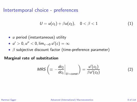
Intertemporal choice - preferences
U = u(c1) + βu(c2), 0 < β < 1 (1)
• u period (instantaneous) utility
• u′ > 0, u′′ < 0, limc→0 u′(c) = ∞
• β subjective discount factor (time-preference parameter)
Marginal rate of substitution
MRS
(≡ −
dc2
dc1
∣∣∣∣U=const
)=
u′(c1)
βu′(c2)(2)
Hartmut Egger Advanced (International) Macroeconomics 8 of 114

C1
C2
Intertemporalindifference curve
Figure 1: Intertemporal indifference curve
Hartmut Egger Advanced (International) Macroeconomics 9 of 114

Example utility functions
• Example 1: u(ct) = ln ct
• Example 2: u(ct) =c1−1/σt
1− 1/σ, 0 < σ(6= 1).
(Isoelastic utility functions)
Hartmut Egger Advanced (International) Macroeconomics 10 of 114

Intertemporal budget constraint
c1 +c2
1 + r= y1 +
y2
1 + r(3)
• r interest rate (if there are variable interest rates, rt+1 denotes
interest rate from t to t + 1 . Thenc2
1 + r2etc.).
• yt endowment (income) in period t.
Hartmut Egger Advanced (International) Macroeconomics 11 of 114
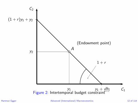
C1
C2
A
(Endowment point)
y1
y2
(1 + r)y1 + y2
y1 +y21+r
1 + r
Figure 2: Intertemporal budget constraint
Hartmut Egger Advanced (International) Macroeconomics 12 of 114

Optimal intertemporal choice
max U s.t. (3)
Lagrange-Function:
L = u(c1) + βu(c2) + λ
(y1 +
y2
1 + r− c1 −
c2
1 + r
)
Hartmut Egger Advanced (International) Macroeconomics 13 of 114
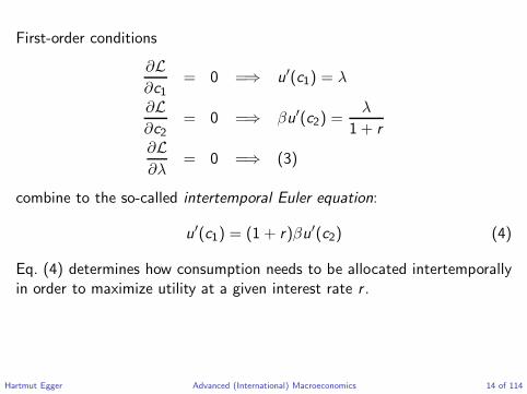
First-order conditions
∂L
∂c1= 0 =⇒ u′(c1) = λ
∂L
∂c2= 0 =⇒ βu′(c2) =
λ
1 + r
∂L
∂λ= 0 =⇒ (3)
combine to the so-called intertemporal Euler equation:
u′(c1) = (1 + r)βu′(c2) (4)
Eq. (4) determines how consumption needs to be allocated intertemporallyin order to maximize utility at a given interest rate r .
Hartmut Egger Advanced (International) Macroeconomics 14 of 114
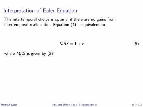
Interpretation of Euler Equation
The intertemporal choice is optimal if there are no gains fromintertemporal reallocation. Equation (4) is equivalent to
MRS = 1 + r (5)
where MRS is given by (2)
Hartmut Egger Advanced (International) Macroeconomics 15 of 114

Equilibrium in an endowmenteconomy
Hartmut Egger Advanced (International) Macroeconomics 16 of 114
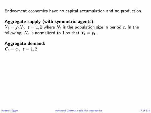
Endowment economies have no capital accumulation and no production.
Aggregate supply (with symmetric agents):Yt = ytNt , t = 1, 2 where Nt is the population size in period t. In thefollowing, Nt is normalized to 1 so that Yt = yt .
Aggregate demand:Ct = ct , t = 1, 2
Hartmut Egger Advanced (International) Macroeconomics 17 of 114

In closed economy (autarky):
Ct = Yt , t = 1, 2 (6)
In open economy:
Ct = Yt + rtBt − CAt (7)
where Bt is the value of net foreign assets inherited from period t − 1 andCAt is the current account balance (Ertragsbilanz, auch Leistungsbilanz).
By definition,CAt = Bt+1 − Bt (8)
Hartmut Egger Advanced (International) Macroeconomics 18 of 114

Remarks on national accounting
• Gross domestic product (GDP) (Bruttoinlandsprodukt): Yt
• Gross national product (GNP) (Bruttosozialprodukt): Yt + rtBt i.e.• GNP=GDP+net international factor payments• net international factor payments here only includes interest and
dividend earnings on net foreign assets• but no workers remittances
• Trade balance (goods and services): Net exports NXt
Hartmut Egger Advanced (International) Macroeconomics 19 of 114
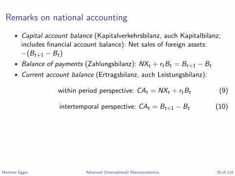
Remarks on national accounting
• Capital account balance (Kapitalverkehrsbilanz, auch Kapitalbilanz;includes financial account balance): Net sales of foreign assets:−(Bt+1 − Bt)
• Balance of payments (Zahlungsbilanz): NXt + rtBt = Bt+1 − Bt
• Current account balance (Ertragsbilanz, auch Leistungsbilanz):
within period perspective: CAt = NXt + rtBt (9)
intertemporal perspective: CAt = Bt+1 − Bt (10)
Hartmut Egger Advanced (International) Macroeconomics 20 of 114

Remarks on national accounting
2013 current account balance in % of GDPSource: Worldbank database
Hartmut Egger Advanced (International) Macroeconomics 21 of 114

Remarks on national accounting
C32 Euro area b.o.p.: current account(seasonally adjusted; 12-month cumulated transactions as a percentage of GDP)
-2.0
-1.0
0.0
1.0
2.0
3.0
2002 2004 2006 2008 2010 2012 2014-2.0
-1.0
0.0
1.0
2.0
3.0
current account balance
Source: ECB.Source: Euro Area statistics online
Hartmut Egger Advanced (International) Macroeconomics 22 of 114

Remarks on national accounting
C33 Euro area b.o.p.: direct and portfolio investment(12-month cumulated transactions as a percentage of GDP)
-2.0
-1.0
0.0
1.0
2.0
3.0
-4.0
-3.0
-2.0
-1.0
0.0
1.0
2.0
3.0
4.0
5.0
2002 2004 2006 2008 2010 2012 2014-4.0
-3.0
-2.0
-1.0
0.0
1.0
2.0
3.0
4.0
5.0
net direct investment
net portfolio investment
Source: Euro Area Statistics online
Hartmut Egger Advanced (International) Macroeconomics 23 of 114

Remarks on national accounting
!"#$
!"%$
!#$
%$
#$
"%$
&%%#$ &%%'$ &%%($ &%%)$ &%%*$ &%"%$ &%""$ &%"&$ &%"+$ &%",$
-./$ 012$ 023$ 42-$ 5/-$ 526$ 178$ 82/$
Current account figures for selected Euro member statesSource: World Development Indicators
Hartmut Egger Advanced (International) Macroeconomics 24 of 114

Remarks on national accounting
Balance of payments of GermanySource: Deutsche Bundesbank: Monthly Report, March 2015
Hartmut Egger Advanced (International) Macroeconomics 25 of 114

Remarks on national accounting
-200
-100
0
100
200
300
400
500
600
700
2007 2008 2009 2010 2011 2012 2013 2014
€b
illi
on
The Bundesbank's TARGET2 balance
Year on year change, net capital exports + year end levels in billion €
Source: Deutsche Bundesbank: Monthly Reports, March 2015
Hartmut Egger Advanced (International) Macroeconomics 26 of 114

Remarks on national accounting
Long-run impact of short-run imbalances:
CAt = NXt + rtBt and CAt = Bt+1 − Bt
implyBt+1 = NXt + (1 + rt)Bt
Repeating the argument for Bt+2 we get
Bt+2 = NXt+1 + (1 + rt+1)NXt + (1 + rt)(1 + rt+1)Bt
Hartmut Egger Advanced (International) Macroeconomics 27 of 114

Remarks on national accounting
In a T + 1-period world with rt = r (inheriting Bt and leaving Bt+T+1):
Bt+T+1 = (1 + r)T+1Bt + (1 + r)TNXt + . . .
+(1 + r)NXt+T−1 + NXt+T
⇐⇒
(1
1 + r
)T
Bt+T+1 = (1 + r)Bt +t+T∑
s=t
(1
1 + r
)s−t
NXs (11)
Hartmut Egger Advanced (International) Macroeconomics 28 of 114
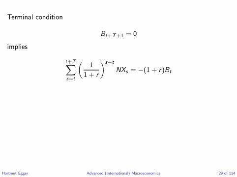
Terminal condition
Bt+T+1 = 0
implies
t+T∑
s=t
(1
1 + r
)s−t
NXs = −(1 + r)Bt
Hartmut Egger Advanced (International) Macroeconomics 29 of 114
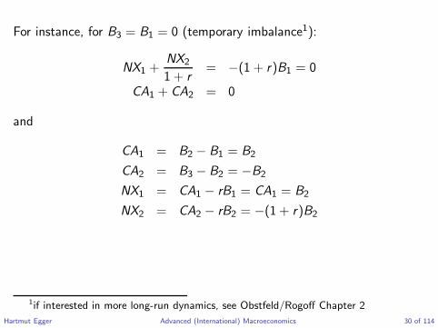
For instance, for B3 = B1 = 0 (temporary imbalance1):
NX1 +NX2
1 + r= −(1 + r)B1 = 0
CA1 + CA2 = 0
and
CA1 = B2 − B1 = B2
CA2 = B3 − B2 = −B2
NX1 = CA1 − rB1 = CA1 = B2
NX2 = CA2 − rB2 = −(1 + r)B2
1if interested in more long-run dynamics, see Obstfeld/Rogoff Chapter 2
Hartmut Egger Advanced (International) Macroeconomics 30 of 114

Equilibrium in a closed economy
Hartmut Egger Advanced (International) Macroeconomics 31 of 114

Goods market equilibrium
Ct = Yt , t = 1, 2
and optimal consumption choice (cf. intertemporal Euler equation)
u′(C1) = (1 + r)βu′(C2)
give us the autarky real interest rate
1 + rA =u′(Y1)
βu′(Y2)(12)
Hartmut Egger Advanced (International) Macroeconomics 32 of 114

(Budget constraint (3) is obviously fulfilled for Ct = Yt .)
• 1 + rA is the willingness to pay for present consumption.
• Virtual price in closed economy without investment possibilities.
• Relevant when opening up.
Hartmut Egger Advanced (International) Macroeconomics 33 of 114
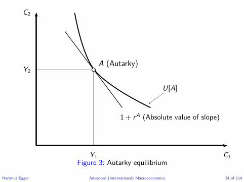
C1
C2
Y1
Y2
A (Autarky)
U[A]
1 + rA (Absolute value of slope)
Figure 3: Autarky equilibrium
Hartmut Egger Advanced (International) Macroeconomics 34 of 114

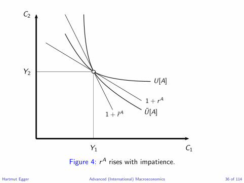
Effect of time preference on rA
β > β implies
MRS(Y1,Y2) < MRS(Y1,Y2)
where MRS(Y1,Y2) ≡u′(Y1)
βu′(Y2)
Hartmut Egger Advanced (International) Macroeconomics 35 of 114
C1
C2
Y1
Y2
1 + rA U[A]
1 + rA
U[A]
Figure 4: rA rises with impatience.
Hartmut Egger Advanced (International) Macroeconomics 36 of 114
Effect of output changes on rA
Assume linear consumption expansion path(MRS(λY1, λY2) = MRS(Y1,Y2))
• rA rises if positive output shock is expected.
• No change of rA if present and future output rise pari passu.
Hartmut Egger Advanced (International) Macroeconomics 37 of 114

C1
C2
Y1
Y2
A1
A2A
1 + rA
1 + rA
1 + rA Expansion path
Figure 5: Effect of output changes on rA
Hartmut Egger Advanced (International) Macroeconomics 38 of 114

Equilibrium in a small openeconomy
Hartmut Egger Advanced (International) Macroeconomics 39 of 114

• 2 periods: B1 = B3 = 0 i.e. NX1 +NX2
1 + r= 0
• r exogenously given by the world market
Intertemporal equilibrium allocation C1,C2 determined by:
u′(C1) = (1 + r)βu′(C2) (13)
C1 +C2
1 + r= Y1 +
Y2
1 + r(14)
Hartmut Egger Advanced (International) Macroeconomics 40 of 114
Special case
If subjective discount factor is equal to market discount factor
β =1
1 + r,
the solution of (13) & (14) is given by
C1 = C2 ≡ C (15)
C =(1 + r)Y1 + Y2
2 + r(16)
For β <1
1 + rthe allocation is biased in favor of C1.
Hartmut Egger Advanced (International) Macroeconomics 41 of 114

Open vs. closed economy equilibrium
C1
C2
C (Open economy equilibrium)
C1
C2
Y1
Y2
(1 + r)Y1 + Y2
Y1 +Y21+r
1 + r
1 + rA
A (Endowment point; Autarky equilibrium)
U[C ]U[A]
NX2
−NX1
Figure 6: Comparing open and closed equilibrium if rA > r
Hartmut Egger Advanced (International) Macroeconomics 42 of 114

• Access to international capital markets allows intertemporal incomeshifting.
• Here from future to present (borrowing) since r < rA.
• Gains from intertemporal trade U [C ] > U [A]
• Debt from current net imports NX1 = Y1 − C1 < 0 must be paidback by future net exports NX2 = −(1 + r)NX1 = Y2 − C2 > 0
Hartmut Egger Advanced (International) Macroeconomics 43 of 114

Implications for trade flows and capital account
According to (7), (9) and (10):
C1 = Y1 + rB1 − CA1 = Y1 + (1 + r)B1 − B2
= Y1 − NX1
C2 = Y2 + rB2 − CA2 = Y2 + (1 + r)B2 − B3
= Y2 − NX2
Hartmut Egger Advanced (International) Macroeconomics 44 of 114
In 2-period world: B1 = B3 = 0
Trade flows
C1 − Y1 = −NX1
Y2 − C2 = (1 + r) (C1 − Y1) = NX2
Net foreign assets
B2 = − (C1 − Y1)
Y2 − C2 = − (1 + r)B2 = (1 + r) (C1 − Y1)
Hartmut Egger Advanced (International) Macroeconomics 45 of 114

“Long-run” effects of short-run trade deficit
If endowment expectations are wrong, the associated short run tradedeficit may have long-run implications (3 or more periods, B1 = 0).
• CA1 = NX1 = B2
• CA2 = rB2 = rNX1
• B3 = CA2 + B2 = (1 + r)NX1
Bt+1 = Bt , t > 3 requires CAt = NXt + rBt = 0
=⇒ For t > 3: NXt = −r(1 + r)NX1 =⇒ Ct(>3) < Yt
B4 = 0 requires CA3 = −B3
=⇒ NX3 = −(1 + r)2NX1 =⇒ C3 < Ct(>3) < Y3
Hartmut Egger Advanced (International) Macroeconomics 46 of 114

Ct
Ct+1
NX2 = 0
Ct(≥3)
C3
A = (A1, A2)ex ante expected
A = (A1,A2)ex post realised
1 + r
C1
(C2 = A2)B3 = (1 + r)NX1
−NX1
Figure 7: “Long-run” effects of trade deficit (3 per., B1 = 0)
Hartmut Egger Advanced (International) Macroeconomics 47 of 114
Intertemporal trade pattern,savings and international
equilibrium
Hartmut Egger Advanced (International) Macroeconomics 48 of 114

Case r < rA
(see figure 6): Implies NX1 < 0, NX2 > 0, given B1 = B3 = 0.
• The country is a net importer in period 1, net exporter in period 2.
• 1 + r is the price of present consumption (here the import good) interms of future consumption (export good).
Hartmut Egger Advanced (International) Macroeconomics 49 of 114

Terms of trade
Terms of trade =price of exports
price of imports=
1
1 + r
decline in r ⇒ i) terms of trade improve
⇒ positive income and wealth effect on C1
ii) substitution effects also favors C1
Hartmut Egger Advanced (International) Macroeconomics 50 of 114
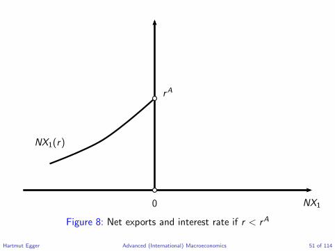
rA
NX1(r)
0 NX1
Figure 8: Net exports and interest rate if r < rA
Hartmut Egger Advanced (International) Macroeconomics 51 of 114
Case r > rA
(see figure 9): Implies NX1 > 0, NX2 < 0, given B1 = B3 = 0.
• Country is net exporter of present output, terms of trade 1 + r
rise in r ⇒ i) positive terms of trade effect on C1
⇒ ii) negative substitution effect on C1
in sum, the NX1-reaction is ambiguous.
Hartmut Egger Advanced (International) Macroeconomics 52 of 114
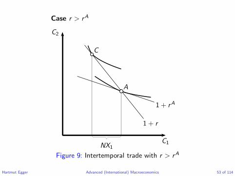
Case r > rA
C2
C1
C
A
1 + r
1 + rA
NX1
Figure 9: Intertemporal trade with r > rA
Hartmut Egger Advanced (International) Macroeconomics 53 of 114

Interest rate
NX1(r)
rA(β,Y2/Y1)(-) (+)
0 NX1(= S1)
Figure 10: Net exports and interest rate if r > rA
Hartmut Egger Advanced (International) Macroeconomics 54 of 114

The position of the curve is fixed by rA.
Remember: rA declines with β and (for linear expansion path ofconsumption) rises with Y2/Y1.
Moreover: For B1 = 0, CA1 = NX1 and thus S1 ≡ Y1 + rB1 − C1 = NX1
Hartmut Egger Advanced (International) Macroeconomics 55 of 114

International equilibrium
Two country world:
Home: rA (β,Y2/Y1)
Foreign: rA∗
(β∗,Y ∗2 /Y
∗1 )
integrated world is like closed economy with goods market equilibriumcondition
Ct + C ∗t = Yt + Y ∗
t
Hartmut Egger Advanced (International) Macroeconomics 56 of 114
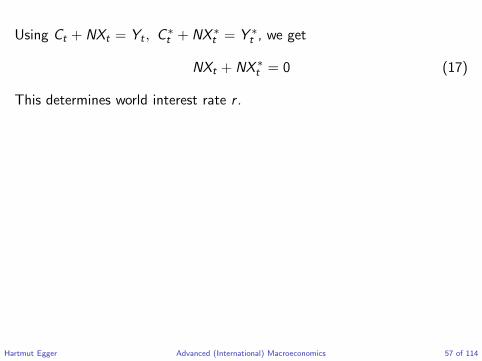
Using Ct + NXt = Yt , C ∗t + NX ∗
t = Y ∗t , we get
NXt + NX ∗t = 0 (17)
This determines world interest rate r .
Hartmut Egger Advanced (International) Macroeconomics 57 of 114

Interest rate
0 NX (r)
NX1(r)
NX ∗1 (r)
rA
rA∗
r
NX1
NX ∗1
Figure 11: Equilibrium world interest rate if rA∗
> rA
Hartmut Egger Advanced (International) Macroeconomics 58 of 114
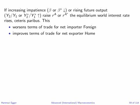
If increasing impatience (β or β∗ ↓) or rising future output(Y2/Y1 or Y ∗
2 /Y∗1 ↑) raise rA or rA
∗
the equilibrium world interest raterises, ceteris paribus. This
• worsens terms of trade for net importer Foreign
• improves terms of trade for net exporter Home
Hartmut Egger Advanced (International) Macroeconomics 59 of 114

Capital accumulation andproduction
Hartmut Egger Advanced (International) Macroeconomics 60 of 114
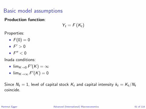
Basic model assumptions
Production function:Yt = F (Kt)
Properties:
• F (0) = 0
• F ′ > 0
• F ′′ < 0
Inada conditions:
• limK→0 F′(K ) = ∞
• limK→∞ F ′(K ) = 0
Since Nt = 1, level of capital stock Kt and capital intensity kt = Kt/Nt
coincide.
Hartmut Egger Advanced (International) Macroeconomics 61 of 114
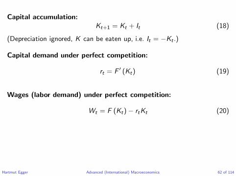
Capital accumulation:Kt+1 = Kt + It (18)
(Depreciation ignored, K can be eaten up, i.e. It = −Kt .)
Capital demand under perfect competition:
rt = F ′ (Kt) (19)
Wages (labor demand) under perfect competition:
Wt = F (Kt)− rtKt (20)
Hartmut Egger Advanced (International) Macroeconomics 62 of 114

Closed economy with capitalaccumulation and production
Hartmut Egger Advanced (International) Macroeconomics 63 of 114
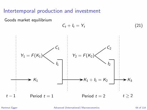
Intertemporal production and investment
Goods market equilibriumCt + It = Yt (21)
Y1 = F (K1) Y2 = F (K2)
C1
I1
C2
I2
K1 K1 + I1 = K2 K3
t − 1 Period t = 1 Period t = 2 t ≥ 2
Hartmut Egger Advanced (International) Macroeconomics 64 of 114
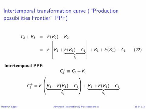
Intertemporal transformation curve (“Production
possibilities Frontier” PPF)
C2 + K3 = F (K2) + K2
= F
K1 + F (K1)− C1︸ ︷︷ ︸
I1
+ K1 + F (K1)− C1 (22)
Intertemporal PPF:C+2 ≡ C2 + K3
C+2 = F
K1 + F (K1)− C1︸ ︷︷ ︸
K2
+ K1 + F (K1)− C1︸ ︷︷ ︸
K2
Hartmut Egger Advanced (International) Macroeconomics 65 of 114

dC+2
dC1= −
1 + F ′
K1 + F (K1)− C1︸ ︷︷ ︸
K2
< 0
d2C+2
dC 21
= F ′′(K2) < 0
Hartmut Egger Advanced (International) Macroeconomics 66 of 114

C1
C+2
X
F (K1 + F (K1)) + K1 + F (K1)
X2 = F (K2) + K2
K1 + I1 = K2 1 + F ′(K2)
X1 F (K1) + K1
Figure 12: Intertemporal production possibilities frontier
Hartmut Egger Advanced (International) Macroeconomics 67 of 114
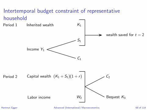
Intertemporal budget constraint of representative
householdPeriod 1 Inherited wealth K1
wealth saved for t = 2
S1
Income Y1
C1
Period 2 Capital wealth (K1 + S1)(1 + r) C2
Labor income W2 Bequest K3
Hartmut Egger Advanced (International) Macroeconomics 68 of 114
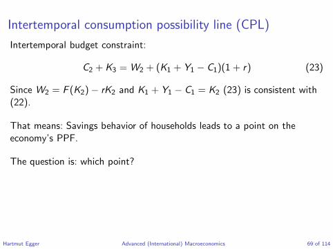
Intertemporal consumption possibility line (CPL)
Intertemporal budget constraint:
C2 + K3 = W2 + (K1 + Y1 − C1)(1 + r) (23)
Since W2 = F (K2)− rK2 and K1 + Y1 − C1 = K2 (23) is consistent with(22).
That means: Savings behavior of households leads to a point on theeconomy’s PPF.
The question is: which point?
Hartmut Egger Advanced (International) Macroeconomics 69 of 114

Optimal intertemporal choice
K3- choice depends on the “bequest” motive. Can be captured by
u(C1) + βu(C+2 )
C+2 = C2 + K3 . . . “bequest” motive
C+2 = C2 . . . no “bequest” motive
max u(C1) + βu(C+2 ) s.t. C+
2 = W2 + (K1 + Y1 − C1)(1 + r)
Hartmut Egger Advanced (International) Macroeconomics 70 of 114

Optimal intertemporal choice yields first-order condition
MRS ≡u′(C1)
βu′(C+2 )
= 1 + r
where K3 = 0 without bequest motive. (K3 = 0 implies K2 + I2 = 0 andthus S2 = I2 = −K2.) In dubio, assume K3 = 0, i.e. C2 = C+
2 in thefollowing.
Hartmut Egger Advanced (International) Macroeconomics 71 of 114

C1
C+2
A
U[A]
F (K2) + K2
K1 + I1 = K2
1 + rA
F (K1) + K1
CPL
PPF
Figure 13: CPL and PPF
Hartmut Egger Advanced (International) Macroeconomics 72 of 114

Small open economy with capitalaccumulation and production
Hartmut Egger Advanced (International) Macroeconomics 73 of 114
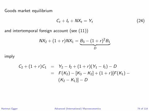
Goods market equilibrium
Ct + It + NXt = Yt (24)
and intertemporal foreign account (see (11))
NX2 + (1 + r)NX1 = B3 − (1 + r)2B1︸ ︷︷ ︸D
imply
C2 + (1 + r)C1 = Y2 − I2 + (1 + r)(Y1 − I1)− D
= F (K2)− [K3 − K2] + (1 + r)[F (K1)−
(K2 − K1)]− D
Hartmut Egger Advanced (International) Macroeconomics 74 of 114

Hence,
C2 + K3︸ ︷︷ ︸C+2
+(1 + r)C1 = F (K2) + K2︸ ︷︷ ︸X2
+(1 + r) [F (K1) + K1 − K2]︸ ︷︷ ︸X1
−D (25)
where X = (X1,X2) is a point at the PPF.
Hartmut Egger Advanced (International) Macroeconomics 75 of 114

C1
C+2
X1
X2
C1
C2
PPF
X
C
CPL(r) given by (25)
1 + r
Figure 14: Consumption possibilities line (CPL) under world interest andD = 0.
Hartmut Egger Advanced (International) Macroeconomics 76 of 114
C1
C+2
D > 0
D = 0D < 0
X
1 + r
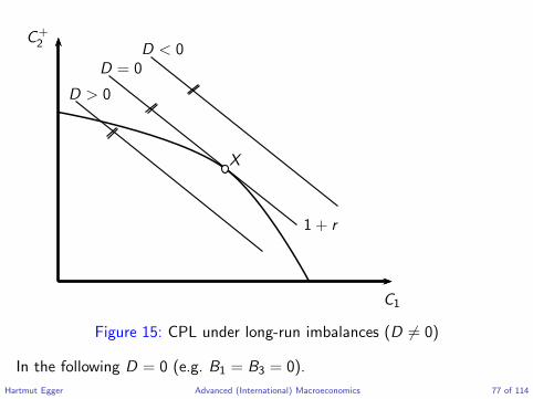
Figure 15: CPL under long-run imbalances (D 6= 0)
In the following D = 0 (e.g. B1 = B3 = 0).
Hartmut Egger Advanced (International) Macroeconomics 77 of 114
C1
C+2
U[C ]
PPF
X
C
1 + r
−NX1
NX2
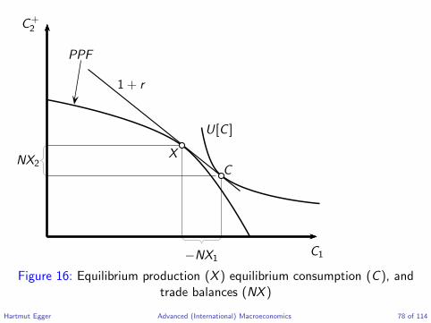
Figure 16: Equilibrium production (X ) equilibrium consumption (C ), andtrade balances (NX )
Hartmut Egger Advanced (International) Macroeconomics 78 of 114

From autarky to open economy equilibriumCase r < rA:
C1
C+2
X
A C
1 + r
1 + rA
∆I1 ∆C1
Figure 17: Double gains from intertemporal trade
Hartmut Egger Advanced (International) Macroeconomics 79 of 114
In addition to the picture for the endowment economy: Productionstructure shifts from A to X by higher investments ∆I1.
Increase in current consumption by ∆C1. Current account deficit−NX1 = ∆I1 +∆C1 paid back by increased future production (+ possiblylower consumption).
Hartmut Egger Advanced (International) Macroeconomics 80 of 114
Case r > rA:
C1
C+2
A
C
A′
X
1 + rNX1
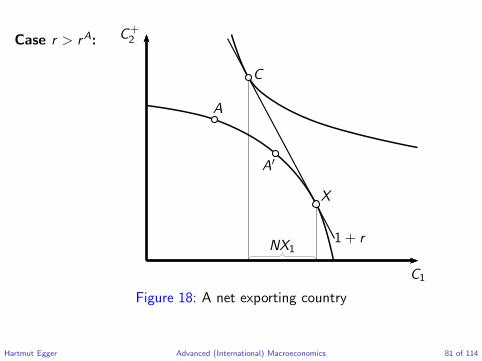
Figure 18: A net exporting country
Hartmut Egger Advanced (International) Macroeconomics 81 of 114
Production shifts in favor of current output by decreasing investment∆I1 < 0. Additional output allows net exports.
Net exports today allow higher future consumption ∆C2 > 0 by futureimports (NX2 = −(1 + r)NX1). Present consumption C1 may shrink (A′)or increase (A) depending on the relative strength of income andsubstitution effect (plus output shift).
Hartmut Egger Advanced (International) Macroeconomics 82 of 114

Adding government consumption
Hartmut Egger Advanced (International) Macroeconomics 83 of 114
With government consumption, period utility has the following additiveform: u(C ) + v(G ). The budget constraint in the two period model is
C1 +C2
1 + r= Y1 − T1 − I1 +
Y2 − T2 − I2
1 + r,
where Tt denotes taxes and Yt − Tt is ‘disposable’ income of the privatesector in period t.
Goods market equilibrium in period t:
Ct + It + Gt + NXt = Yt (26)
Hartmut Egger Advanced (International) Macroeconomics 84 of 114

Current account balance (recall (9),(10)):
CAt = NXt + rBt
= Yt + rBt − Ct − Gt − It
= Yt + rBt − Ct − Tt︸ ︷︷ ︸SPt private savings
+ Tt − Gt︸ ︷︷ ︸public savings
−It
With a balanced budget Tt = Gt of the public sector, private savings areequal to total savings (SP
t = St) and
CAt = SPt + Tt − Gt︸ ︷︷ ︸St total savings
−It (27)
Bt+1 = Bt + St − It (28)
Hartmut Egger Advanced (International) Macroeconomics 85 of 114
Impact of G in small open economy
Increase in G1(G2) shifts transformation curve (PPF) for private sectorleftward (downward).
In the following illustration (with a balanced budget of the government:Tt = Gt):
Initial situation: G1 = G2 = 0 and NX1 = NX2 = 0
Shock 1: G1 ↑
Shock 2: G2 ↑
Hartmut Egger Advanced (International) Macroeconomics 86 of 114

C1
C+2
A
CB
1 + r
−NX1
Figure 19: Impact of G1
Hartmut Egger Advanced (International) Macroeconomics 87 of 114

Impact of G1:
• Private feasible output shifts from A to B .
• Would decrease C1 by the full amount of G1 = BA leaving C2
unaffected
• Individuals prefer C by borrowing from abroad.
Hartmut Egger Advanced (International) Macroeconomics 88 of 114
C1
C+2
AC
B
NX1
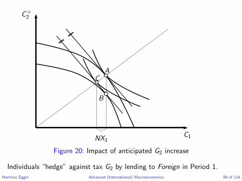
Figure 20: Impact of anticipated G2 increase
Individuals “hedge” against tax G2 by lending to Foreign in Period 1.
Hartmut Egger Advanced (International) Macroeconomics 89 of 114

Investment, savings and worldinterest rate in international
equilibrium
Hartmut Egger Advanced (International) Macroeconomics 90 of 114
The investment function
Production function:Yt = AtF (Kt)
At : Productivity parameter
Accumulation equation:
K2 = K1 + I1
In the following, we consider a 2-period model with B1 = B3 = 0, K3 = 0and Gt = Tt = 0.
Hartmut Egger Advanced (International) Macroeconomics 91 of 114

Condition for optimal capital input under perfect competition:
r = A2F′(K1 + I1) (29)
(29) defines investment curve
I1 = I (r/A2), I′
< 0
The negative slope follows from F ′′ < 0.
Hartmut Egger Advanced (International) Macroeconomics 92 of 114
I1
r
rA
I for A2 I for A2 > A2
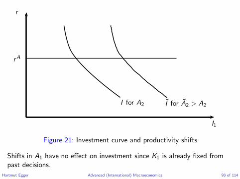
Figure 21: Investment curve and productivity shifts
Shifts in A1 have no effect on investment since K1 is already fixed frompast decisions.
Hartmut Egger Advanced (International) Macroeconomics 93 of 114
The saving function
Reconsidering the endowment economy: From the endowment economywe know that B1 = B3 = 0 implies S1 = Y1 − C1 = NX1(r).
Furthermore, we can note that, dS1/dr = dNX1/dr = −dC1/dr .
To determine the impact of interest rate r on savings (or, equivalently,NX1), we can first look at the intertemporal Euler equationu′(C1) = (1 + r)βu′(C2).
Substituting the budget constraint C2 = (1 + r)(Y1 − C1) + Y2 gives
u′(C1) = (1 + r)βu′ ((1 + r)(Y1 − C1) + Y2) . (30)
Hartmut Egger Advanced (International) Macroeconomics 94 of 114

Implicitly differentiating (30) with respect to r gives
dC1
dr=
βu′(C2) + β(1 + r)u′′(C2)(Y1 − C1)
u′′(C1) + β(1 + r)2u′′(C2). (31)
Noting u′ > 0, u′′ < 0, it is immediate that dNX1(r)/dr = −dC1/dr > 0 ifC1 > Y1 (or, equivalently, NX1 < 0).
However, dNX1(r)/dr = −dC1/dr < 0 cannot be ruled out if Y1 > C1 (or,equivalently, NX1 > 0) – see Figure 10.
Hartmut Egger Advanced (International) Macroeconomics 95 of 114

Consumption in a model with capital accumulation and productionSubstituting the budget constraint
C2 = (1 + r)[A1F (K1)− C1 − I1] + A2F (K1 + I1) + K1 + I1
for C2 in the Euler equation u′(C1) = (1 + r)βu′(C2), gives
u′(C1) = (1 + r)βu′ {(1 + r)[A1F (K1)− C1 − I1]
+A2F (K1 + I1) + K1 + I1} . (32)
Implicitly differentiating with respect to r yields
dC1
dr=
βu′(C2) + β(1 + r)u′′(C2) [A1F (K1)− C1 − I1]
u′′(C1) + β(1 + r)2u′′(C2)
+β(1 + r)u′′(C2) {A2F
′(K1 + I1)− r} ∂I/∂r
u′′(C1) + β(1 + r)2u′′(C2).
Hartmut Egger Advanced (International) Macroeconomics 96 of 114

Accounting for A2F′(K1 + I1) = r further implies
dC1
dr=
βu′(C2) + β(1 + r)u′′(C2) [A1F (K1)− C1 − I1]
u′′(C1) + β(1 + r)2u′′(C2). (33)
Hence, the derivative in (33) is precisely the same as the derivative in(31), but with Y1 − C1 replaced by the date 1 current account for aninvestment economy with B1 = 0: A1F (K1)− C1 − I1.
That means that, given current account balances, the slope of the savingschedule is the same as for the endowment economy!
Hartmut Egger Advanced (International) Macroeconomics 97 of 114

An intuition for this resultThe symmetry in the reaction of savings to interest rate adjustments inthe endowment and the investment economy is a consequence of theenvelope theorem.
The first-order condition for profit-maximizing investment ensures that asmall deviation from optimum investment does not alter the present valueof national output, evaluated at the world interest rate.
Consequently, at the margin, the investment adjustment ∂I1/∂r has noeffect on net lifetime resources, and hence no effect on consumptionresponse.
Hartmut Egger Advanced (International) Macroeconomics 98 of 114

From consumption to savingAs noted above, savings in period 1 are given by S1 = Y1 − C1 or,equivalently, S1 = A1F (K1)− C1. Hence, we can write savings as functionof r , A1, A2 and β:
S1 = S(r ,A1,A2, β),
with ∂S1/∂r > 0 in the regular (non-perverse) case.
Saving curve and productivity shiftAn increase of At has analogous effects to an increase of Yt in endowmenteconomy.
• According to slide 54 a rise in Y1 shifts the S-curve to the right. A rise in Y2
shifts the S-curve to the left.
• Rising impatience (a fall in β) also shifts the saving curve to the left.
Hartmut Egger Advanced (International) Macroeconomics 99 of 114

S1
r
rA
S for A1,A2, β S for A1 > A1
A2 < A2
β > β
Figure 22: Saving curve
Hartmut Egger Advanced (International) Macroeconomics 100 of 114

Investment, savings and current account
S1, I1
r
rA
S
I−CA1 = I1 − S1
CA1 = S1 − I1
Figure 23: Investment, savings and current account
Hartmut Egger Advanced (International) Macroeconomics 101 of 114
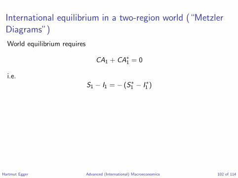
International equilibrium in a two-region world (“Metzler
Diagrams”)
World equilibrium requires
CA1 + CA∗1 = 0
i.e.S1 − I1 = − (S∗
1 − I ∗1 )
Hartmut Egger Advanced (International) Macroeconomics 102 of 114

r r
rA
rrA
∗
A B
S I
Home
A∗
B∗
S∗I ∗
Foreign
CA1
−CA∗1
Figure 24: World equilibrium interest rate rA < r < rA∗
Hartmut Egger Advanced (International) Macroeconomics 103 of 114
r r
rr
S I
Home
S∗S∗
I ∗
Foreign
CA1
CA1
−CA∗
1
−CA∗1
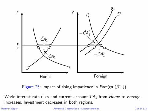
Figure 25: Impact of rising impatience in Foreign (β∗ ↓)
World interest rate rises and current account CA1 from Home to Foreign
increases. Investment decreases in both regions.
Hartmut Egger Advanced (International) Macroeconomics 104 of 114

Impact of positive productivity shock in Foreign
Consider a productivity shock of the form A∗2 ↑
World interest rate rises
In Home Investment fallsSaving and CA1-surplus rise
In Foreign Investment reaction ambiguousCA∗
1-deficit rises
Hartmut Egger Advanced (International) Macroeconomics 105 of 114

r r
r
r
S I
Home
S∗S∗
I ∗I ∗
Foreign
CA1
CA1
−CA∗
1−CA∗
1
Figure 26: Impact of positive productivity shock in Foreign
Hartmut Egger Advanced (International) Macroeconomics 106 of 114

Stability of international equilibrium and Marshall-Lerner
condition
The world equilibrium condition CAt + CA∗t = 0 is
St(r) + S∗t (r) = It(r) + I ∗t (r) (34)
(Use CAt = St − It)
As addressed in Figure 10, the saving curve may be backward bending, sothat multiple equilibria and unstable equilibria cannot be excluded.
Hartmut Egger Advanced (International) Macroeconomics 107 of 114

(Walrasian) stability condition: A market is stable in the Walrasian sense ifa small increase in the price of the good traded there causes excess supply,while a small decrease causes excess demand.
The stability condition defining Walrasian stability in the market for worldsavings is that a small rise in r should lead to an excess supply of savings:
d [S1(r) + S∗1 (r)]
dr>
d [I1(r) + I ∗1 (r)]
dr(35)
Stability guarantees that market forces tend to eliminate imbalancesresulting from small disturbances of international equilibrium.
Hartmut Egger Advanced (International) Macroeconomics 108 of 114

World saving and investment
r
r
S + S∗
I + I ∗
Figure 27: Savings and Investment
Hartmut Egger Advanced (International) Macroeconomics 109 of 114

For B1 = B3 = 0 national accounting identities imply
NX1 = CA1 = S1 − I1NX ∗
1 = CA∗1 = S∗
1 − I ∗1
Moreover (see (11)),
NX ∗1 +
NX ∗2
1 + r= 0
Hartmut Egger Advanced (International) Macroeconomics 110 of 114

Using this in international equilibrium condition (34), we get
S1 − I1 + S∗1 − I ∗1 = NX1 −
NX ∗2
1 + r
Thus (35) is equivalent to
d
[NX1(r)−
NX ∗2 (r)
1 + r
]
dr> 0 (36)
Hartmut Egger Advanced (International) Macroeconomics 111 of 114
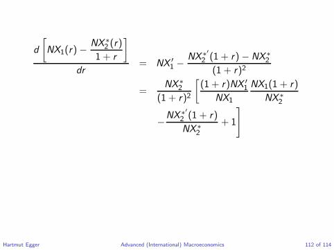
d
[NX1(r)−
NX ∗2 (r)
1 + r
]
dr= NX ′
1 −NX ∗′
2 (1 + r)− NX ∗2
(1 + r)2
=NX ∗
2
(1 + r)2
[(1 + r)NX ′
1
NX1
NX1(1 + r)
NX ∗2
−NX ∗′
2 (1 + r)
NX ∗2
+ 1
]
Hartmut Egger Advanced (International) Macroeconomics 112 of 114

In equilibrium NX1(1 + r) = −NX2 = NX ∗2 . Thus the square bracket is
negative (positive) if
−(1 + r)NX ′
1
NX1︸ ︷︷ ︸η
+(1 + r)NX ∗′
2
NX ∗2︸ ︷︷ ︸
η∗
> (<) 1 (37)
If Home is net importer today (NX1 < 0), then NX ∗2 < 0 and stability
condition (35) is equivalent to
η + η∗ > 1. (38)
Hartmut Egger Advanced (International) Macroeconomics 113 of 114

Interpretation (NX1 < 0)η is the (absolute value of) negative import elasticity of Home withrespect to price 1 + r of current consumption. η∗ is the (positive) elasticityof Foreign’s future imports. (38) is the intertemporal analogue to theso-called Marshall-Lerner condition.
RemarkWhen Home happens to be the exporter in period 1, rather than theimporter, (38) still characterizes the Walras-stable case, but with importelasticities defined so that Home’s and Foreign’s role are interchanged.
Hartmut Egger Advanced (International) Macroeconomics 114 of 114