International Journal of Systems Science Modelling

PLEASE SCROLL DOWN FOR ARTICLE

This article was downloaded by: [Massachusetts Institute of Technology, MIT Libraries]On: 6 January 2011Access details: Access Details: [subscription number 922844579]Publisher Taylor & FrancisInforma Ltd Registered in England and Wales Registered Number: 1072954 Registered office: Mortimer House, 37-41 Mortimer Street, London W1T 3JH, UK

International Journal of Systems SciencePublication details, including instructions for authors and subscription information:http://www.informaworld.com/smpp/title~content=t713697751

Modelling electrocardiograms using interacting Markov chainsPeter C. Doerschuka; Robert R. Tenneyb; Alan S. Willskya

a Laboratory for Information and Decision Systems, Massachusetts Institute of Technology,Cambridge, MA, U.S.A. b Alphatech, Inc., 2 Burlington Executive Center, Burlington, MA, U.S.A.

To cite this Article Doerschuk, Peter C. , Tenney, Robert R. and Willsky, Alan S.(1990) 'Modelling electrocardiogramsusing interacting Markov chains', International Journal of Systems Science, 21: 2, 257 — 283To link to this Article: DOI: 10.1080/00207729008910361URL: http://dx.doi.org/10.1080/00207729008910361

Full terms and conditions of use: http://www.informaworld.com/terms-and-conditions-of-access.pdf

This article may be used for research, teaching and private study purposes. Any substantial orsystematic reproduction, re-distribution, re-selling, loan or sub-licensing, systematic supply ordistribution in any form to anyone is expressly forbidden.

The publisher does not give any warranty express or implied or make any representation that the contentswill be complete or accurate or up to date. The accuracy of any instructions, formulae and drug dosesshould be independently verified with primary sources. The publisher shall not be liable for any loss,actions, claims, proceedings, demand or costs or damages whatsoever or howsoever caused arising directlyor indirectly in connection with or arising out of the use of this material.

http://www.informaworld.com/smpp/title~content=t713697751

http://dx.doi.org/10.1080/00207729008910361

http://www.informaworld.com/terms-and-conditions-of-access.pdf

Modelling electrocardiograms using interacting Markov chains

PETER C. DOERSCHUKt . ROBERT R. TENNEYf. and ALAN S. WILLSKY7

A methodology is developed for the statistical modelling of cardiac behaviour and electrocardiograms (ECGs) that emphasizes (o) the physiological event/detailed waveform hierarchy; and ( b ) the importance orcontrol and timing i n describing the interactions among the several anatomical sub-units ofthc heart. This methodology has been motivated by a desire to develop improved algorithms for statistical rhythm analysis. Specifically, to develop algorithms that capture cardiac behaviour in a more fundamental way but that stop short of complete accuracy in order to highlight decompositions that can be exploited to simplify statistical inlerencc based on these models. Our models consist of interacting linite-state processes, where a very few olthe transition probabilities for each process can take on a small number oldikrent values depending upon the states ofneighbouring processes. Each finite- state process is constructed from a very small set of elementary structural elements. We illustrate our methodology by describing models for three cardiac rhythms and include simulation results for one or these, namely the rhythm known as Wenckebach.

1. Introduction In this paper we describe a methodology lor the statistical modelling of cardiac

activity and electrocardiograms (ECGs). O u r primary purpose in developing this methodology is to provide a basis for the design of automatic, statistical algorithms for rhythm analysis of ECGs, that is, the analysis of the sequential behaviour of both atrial and ventricular events as observed in the ECG (Doerschuk er al. 1990).

Modelling of ECGs is certainly not a new endeavour (see Thomas er (11 . 1979, Feldman and Hubelbank 1977, Oliver er a/ . 1977, Leblanc and Roberge 1973, Cox er ul. 1972) nor is the development of statislical ECG models for the express purpose of designing signal analysis algorithms. However, the modelling methodology we describe here differs in a number of important ways from any earlier work. Roughly speaking, we have tried, on the one hand, to overcome the limitations ofexisting signal processing models by capturing cardiac physiology in a far more fundamenlal way. O n the other hand, we have stopped far short of the detail found in physiologically- accurate models and rather have aimed both to keep only enough detail to allow successful signal processing and to highlight several critical features found in physiological models that allow the development of computationally feasible algorithms.

In particular, as we briefly describe in the next section, the behaviour of the heart is characterized by the occurrence of a small number of events corresponding to

Received 5 June 1989. t Laboratory for lnformation and Decision Systems, Massachusetts Institute or Tech-

nology. Cambridge, MA 02139, U.S.A. f Laboratory for lnformation and Decision Systems. Massachusetts Institute of Tech-

nology. Cambridge, MA 02139, U.S.A., and Alphatech, Inc.. 2 Burlington Executive Center, l l I Middlesex Tpke., Burlington, MA 01803, USA.

Downloaded By: [Massachusetts Institute of Technology, MIT Libraries] At: 16:49 6 January 2011

258 P. C. Doerschuk et al

contraction or relaxation of different major parts of the heart, and each of these events leads to the appearance of a particular waveform in the ECG. While very accurate descriptions of the ECG require breaking the ECG down further to account for the behaviour of very small units of heart muscle, one can generally think of describing the ECG in hierarchical fashion-an upper level describing discrete cardiac events and a lower level describing the impact these events have on the ECG. As we discuss in 5 2, previously developed rhythm analysis methods typically make use of this decomposition implicitly-i.e. only the event level description is modelled, and i t i s assumed that a wave detection preprocessor has been applied to the ECG to provide event- level inputs to the signal processing algorithms. Our approach differs from these in two important ways. I n the first place, we explicitly model the two-level hierarchy, thereby allowing an integrated approach to wave detection and rhythm tracking. This provides a fundamental way to feed rhythm information back to the wave detection process. Secondly, and more importantly, our event-level descriptions of cardiac behaviour are far more detailed and accurate than those used previously. I n particular, the heart consists of several distinct sub-units which interact relatively infrequently but strongly. Furthermore, the coordinated action of the heart (or any particular anomaly) can be explained in terms of control and timing. Specifically, the contraction of one part of the heart initiates the contraction of a neighbouring portion (and thereby controls i t s behaviour) i f that portion of the heart i s ready lo contract (i.c. i f the timing i s right). As we describe, these observations plus a detailed examination of the mechanisms that characterize different cardiac rhythms have led us to develop a methodology for constructing spatially distributed models of cardiac behaviour, emphasizing control and timing, and using a very small number of building blocks.

This paper i s organized as follows: in the next section we provide a brief introduction to cardiac anatomy and physiology, review previous cardiac modelling investigations, and present an introduction to our modelling methodology. Sections 3 and 4 describe the general mathematical structure of the upper and lower levels, respectively, ofour models, and in 3 5 we describe in detail the building blocks used to construct our upper level models. In 9 6 we present three examples of rhythm models using our methodology, including the complete details and some simulations for one of these, namely the rhythm known as Wenckebach (5 6.3).

2. Cardiac anatomy, physiology, and modelling I n this section we summarize the physiological basis of our models, review some of

the literature on ECG modelling, and present an overview of our model. The heart pumps blood by coordinated muscular contraction. The coordination i s achieved by waves ofdepolarization that propagate in the cell membranes of a conduction system embedded in the muscular and structural elements of the heart and in the muscle cells themselves. The voltage fluctuations measured at the surface of the chest due to these depolarization waves are the ECG. After a depolarization wave passes through a patch of membrane, the patch must be repolarized before i t i s able to support a second wave. The period of time during which i t i s unable to support a depolarization wave i s called the refractory period. Many parts of the heart depolarize periodically without external stimulation and are called autorhythmic.

A normal heart beat is initiated by an autorhythmic depolarization of the sino- atrial (SA) node. The depolarization propagates into the atria, causing the P-wave in the ECG (see Fig. I) and causing the atria to contract and pump their contents into


Mod~lling ~lccrrocordiogrum.~ ~rsir~g i~~rertrcring Morkou chains 259

Figure I . Waveform definitions for one beat of an idealized normal ECG.

the ventricles. The depolarization wave thcn propagates through the atrio-ventricular (AV) node which is the only electrical connection in the normal heart between the atria and ventricles and which delays the wave by 70-80 ms thereby allowing the blood pumped out of the atria to fill the ventricles before the ventricles contract. Findly, the depolarization wave propagates through the specialized ventricular conduction system and ventricular muscle causing the major R- and minor Q- and S-waves in the ECG and causing the ventricles to pump their contents into the lungs and systemic body. Because the ventricles have a greater mass of muscle than the atria, the R-wave is greater in amplitude than the P-wave. Finally. the ventricular muscle rcpolarizes causing the T-wave in the ECG. (The ECG wave caused by the repolarization of the atria is masked by the much larger R-wave.)

Though the preceding description of cardiac functioning is simplified, we believe that not much additional complexity is required in order to model a wide variety of cardiac rhythms. Specifically, there are a small number of general mechanisms present in a physiologically normal heart which, when combined with three broad categories of physiological abnormalitics, lead to a wide variety of arrhythmias.

The first normal mechanism concerns autorhythmicity. The frequency of autorhythmic depolarization varies with anatomic location and is greater in more proximal structures. (Structure A is proximal to structure B if it occurs before structure B in the normal depolarization scquence. The reverse of proximal is distal.) This association between loc;~tion and frequency is called the gradient of autorhythmicity. When an autorhythmic structure is depolarized by an external source, the biological clock counting down to the next spontaneously generated depolarization is reinitialized. The time interval between the reinitialization and the next spontaneous depolarization may simply be the usual autorhythmic period, in which case the process is called resetting, o r it may be somewhat longer, in which case the process is called stunning. In light of the gradient of autorhythmicity and the reset/stun phenomena, the SA node is generally able to win the competition with more distal autorhythmic centres for control of the normal heart.

What we have just described is the unidirectional propagation of the depolarization wave through the heart in the normal direction, called the antegrade direction. Another normal mechanism in the cardiac conduction system is that i t is also capable of propagation in the reverse, or retrograde, direction. This is obviously important when depolarizations are initiated in distal structures.

Let us now turn to the three categories of physiological abnormalities:

(o) decreased conduction capabilities

( h ) increased or decreased rates of autorythmicity


260 P. C. Doerschuk et al.

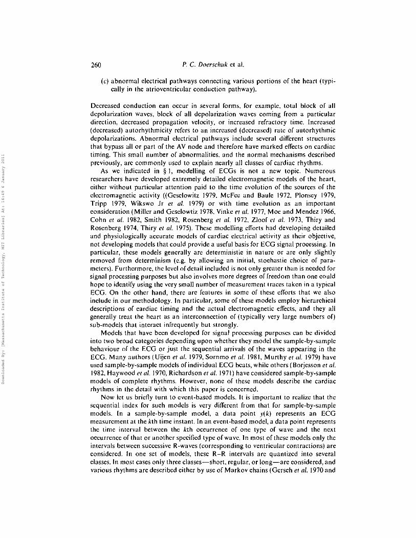
(c) abnormal electrical pathways connecting various portions of the heart (typically in the atrioventricular conduction pathway).

Decreased conduction can occur in several forms, for example, total block of a l l depolarization waves, block of all depolarization waves coming from a particular direction, decreased propagation velocity, or increased refractory time. Increased (decreased) autorhythmicity refers to an increased (decreased) rate of autorhythmic depolarizations. Abnormal electrical pathways include several different structures that bypass all or part of the AV node and therefore have marked effects on cardiac timing. This small number of abnormalities. and the normal mechanisms described previously, are commonly used to explain nearly all classes of cardiac rhythms.

As we indicated in 5 1, modelling of ECGs is not a new topic. Numerous researchers have developed extremely detailed electromagnetic models of the heart. either without particular attention paid to the time evolution of the sources of [he electromagnetic activity ((Geselowitz 1979. McFee and Baulc 1972, Plonsey 1979. Tripp 1979, Wikswo Jr er ul. 1979) or with time evolution as an important consideration (Miller and Geselowtiz 1978. Vinke er id. 1977, Moe and Mendez 1966. Cohn er ul. 1982, Smith 1982, Rosenberg er ul. 1972, Zloof er ul. 1973, Thiry and Rosenberg 1974, Thiry er a/. 1975). These modelling elTorts had developing detailed and physiologically accurate models of cardiac electrical activity as their objective, not developing models that could provide a useful basis for ECG signal processing. In particular, these models generally are deterministic in nature or are only slightly removed from determinism (e.g. by allowing an initial, stochastic choice of parameters). Furthermore, the level ofdetail included i s not only greater than is needed for signal processing purposes but also involves more degrees offreedom than one could hope to identify using the very small number of measurement traces takcn in a typical ECG. On the other hand, there arc features in some of these efforts that we also include in our methodology. In particular, some of these models employ hierarchical descriptions of cardiac timing and the actual electromagnetic effects, and they al l generally treat the heart as an interconnection of (typically very large numbers of) sub-models that interact infrequently but strongly.

Models that have been developed for signal processing purposes can be divided into two broad categories depending upon whether they model the sample-by-sample behaviour of the ECG or just the sequential arrivals of the waves appearing in the ECG. Many authors (Uijen era / . 1979, Sornmo er nl. 1981, Murthy er (11. 1979) have used sample-by-sample models of individual ECG beats, while others (Borjesson et a/. 1982. Haywood rr (11. 1970, Richardson el 01. 1971) have considered sample-by-sample modcls of complete rhythms. However, none of these models describe the cardiac rhythms in the detail with which this paper i s concerned.

Now let us briefly turn to event-based models. I t i s important to realize that the scqucntial index for such modcls i s very different from that for sample-by-sample models. In a sample-by-sample model, a data point y(k) represents an ECG measurement at the kth time instant. I n an event-based model, a data point represents the time intcrvnl between the kth occurrence of one type of wave and the next occurrence ofthat or another specified type of wave. I n most of these models only the interv:ds between successive R-waves (corresponding to ventricular contractions) are considered. In one set of models, these R-R intervals are quantized into several classes. In most cases only three classes-short, regular, or long-are considered, and various rhythms are described either by use of Markov chains (Gersch er al. 1970 and


Modellitlg elecrrocurdiogru~ns using inrerocring Murkou chains 26 1

1975, Tsui and Wong 1975, Shah rr 01. 1977, White 1976) or deterministic finite automata (Hristov 1971) to model the evolution of R-R interval patterns. I n another set of papers (Gustafson er al. 1978, 1981) interval lengths are not quantized, and an extensive set of vector Markov models are developed to describe the evolution of event interval patterns (see Ciocloda 1983 for an independent, though less compre- hensive, development). In the first part of this work (Gustafson er al. 1978) only R-R intervals are considered, while P-R intervals are also considered in the later paper.

From the perspective of the approach in this paper, these event-oriented models do highlight the timing information, which i s of primary importance in tracking or identifying cardiac rhythms. Howwer, the use of purely event-based models has some fundamental limitations. In 5 1 we mentioned one of these, namely the implicit :issumption that wave detection has already been performed in a prc-processor. As we indicated, one might expect superior performance in an integrated algorithm in which rhythm tracking information assists wave detection. Only in Gustafson er al. (1981) docs one not find an ( d koc) use of feedback from tracker to wave detector. While the absence ol;i fundamental way in which to effect this feedback i s a limitation, i t i s not the most serious one. A more basic problem with event-based models i s the limited way in which one must model pre-processor errors. Specifically, this framework allows onc to model the error in measuring the interval between two events, but it cannot :iccommodate the possibility that one of these events i s missed altogether by the preprocessor. While this i s not a serious problem for the large-amplitude QRS complex, i t i s a problem lor the much smaller P-wave. The difficulty here i s with the sequential event-related index. which also creates another even more serious problem. In p:irticular, in many cardiac rhythms, such as those involving some type of AV node abnormality that on occasion causes a ventricular contraction to be dropped, there i s a ooriuhle number of P-waves between successive R-waves. For rhythms such as these, the use of an event-oriented time index breaks down. or at best leads to models with a tenuous connection to actual cardiac behaviour.

From the preceding discussion, the hierarchical nature of the ECG is apparent- an upper level describing events and a lower level describing the waveforms resulting from events. Also apparent i s the spatially-distributed nature of the ECG and the role of control and timing in the interactions between the spatially-distributed compo- nents. Here, by control, we mean one portion of the heart triggering activity in another portion and, by timing, we mean the fact that the effect of this triggering may depend upon the state of the receiving portion. Finally. though we have not emphasized i t in the previous discussion, there i s a temporal decomposition. Specifically. the spatial decomposition of the heart into sub-units which interact strongly but at infrequent intervals compared to the time scale at which each subunit evolves.

I n our approach to cardiac modelling. we highlight the occurrence of cardiac events. as has been done in previous signal processing models. However we hwe. at the same time, avoided the difficulties described previously by basing our models Far more closely on cardiac physiology and anatomy. The key to accomplishing this in an eRective way is to rely heavily upon and to highlight the spatial, temporal, and hierarchical aspects of cardiac phenomenology that we have just described.

Figure 2 presents a three-sub-model example of the type of model we consider. The square boxes at the upper level of the hierarchy comprise the discrete-state physiological model, which captures the sequential evolurion of high level events in the heart. The mathematical structure of these models i s described in Q: 3. Each sub-model


P. C. Doersckuk et al.

i I I

ECG

Figure 2. Spatial and hierarchical decompositions.

represents a functional anatomic structure (e.g. the atria, the ventricles, etc.). The directed solid lines indicate the initiator and rec~pient of control inputs, which we call intcr:wxions. For example, the transmission ofa depolarization wave from atria to AV node might be modelled via an interaction in which the present state of a sub-model representing the atria causes a transition in the AV-nodal sub-model, representing the initiation of the AV-nodal depolarization.

The triangular objects in Fig. 2 are parts of the electromagnetic model which models the actual observed weveforms. Each sub-model corresponds to the gen- erxtion of the ECG contribution from a particular anatomic structure of the heart (e.g. P-waves from the atria). The dashed lines indicate the control of the electromagnetic level by the physiological level o f a single sub-model. These inputs are used to initiate the gcneration of waveforms in the observed ECG. For example, the occurrence of a particular trmsition in the physiological portion of an atrial sub- model might initiate the gcncration ofa P-wave in the corresponding electromagnetic sub-model. The mathematical structure ofthe electromagnetic level i s described in 5 4. Note that the electromagnetic level does not affect the physiological level and that there arc no interactions among electromagnetic sub-models.

Finally it is very important to notc that often it i s the interactions between the normal and abnormal parts of the heart that are of critical importance. That is, many of the changes in an arrhythmic ECG are due to how an abnormal sub-structure aRects a normal part of the heart, rather than to a direct change in the ECG caused by the depolarization of the abnormal sub-structure. For example, the existence of a faster clcctrical connection bclween atria and ventricles leads to marked changes in the timing ofthe P- and QRS-waves and possibly to abnormal QRS complexes, even though the atria and ventricles are perfectly normal.


Modelling elecrrocardiograms using interacring Markov chains 263

In our models of arrythmias, we take the same approach. That is, we begin with a normal rhythm model which is transformed into an arrythmia model by altering the appropriate sub-model. The contribution of the altered sub-model and its interactions with the unaltered sub-models create the arrythmic ECG. In order for the interactions to occur, we often must generalize the normal sub-models. The alterations are to include properties which were left out initially because, in the normal rhythm, they represented unnecessary detail.

3. Upper hierarchical level In this section we discuss the upper hierarchical level, which we call the

physiological model. This level is concerned with discrete events, and we have chosen to use Markov chains to describe their evolution. Because of the importance of spatial decompositions, we have also chosen a highly structured class of chains described in the following.

The state space of our Markov chains is the cross product of a set of spaces corresponding to the 'states* of sub-processes which comprise the overall chain. Each sub-process corresponds to one of the anatomic sub-units of the heart. Furthermore, there is a direct correspondence between each state of a sub-process and a physical state of the corresponding anatomic sub-unit. We call each sub-process a sub-model.

Let a, be the state of the overall Markov chain which consists of a set of N sub- processes denoted xL, i=O, ..., N - I. A key feature of our models is that the transition density, p(x.+, I.\..), has a great deal of structure. Specifically:

(n) Given x,, the transitions of each of the component sub-processes are independent. That is,

(b) For each sub-process there are far fewer values of

than there are values of {x i , j # i} That is, we assume that

where

denotes the net interaction of all other sub-processes with the ith sub-process. Typically the number of possible values of I(, is quite small. In fact, in our

examples 11: takes on at most two or three values and only one or two transition probabilities of the ith chain are affected by the value of hb. Thus, the sub-processes are 'almost' independent, but, as we will see, these interactions can have an extremely important effect on the evolution of the sub-processes.

We now consider a very simple model for normal rhythm in order to fix these ideas about interacting sub-processes. This model has two sub-models (Fig. 3(a)), corresponding to a division of the heart into two anatomic sub-structures: the SA-atrial (SA/A) sub-structure, composed of the SA node and atria, and the AV-ventricular


P. C. Doerschuk et al

sub-model

AV-ventricles sub-model (sub-model 1)

Electromagnetic sub-model: P wove

I f the s l o l e o f the SA-at r ia l sub-model e (1. 2. 3.4):

I f the stale ol lha SA-atr ial sub-model a {I]:

rub-model ORS complel and

I T wave I

Figure 3. Simple model lor normal rhythm. ( a ) Sub-model block diagram. (h ) SA-atrial sub- model. ( c ) AV-ventricular sub-model.

(AV/V) sub-structure, composed of the A V junction and ventricles. As in the normal heart, the SA/A sub-model originates interactions with the AV/V sub-model, corresponding to a super-ventricular depolarization originating in the SA node and propagating through the AV junction in the antegrade direction. For simplicity, the rcverse (retrograde) conduclion i s not modelled.

In the S/A sub-model (Fig. 3(b)), the state transition from 0 to I represents the firing of the SA node and the atrial depolarization. The time required for the state to travel from state 1 to state 0 models the random time between successive depolariza- lions of the autorhythmic SA node. Finally, by assuming that the atrial conduction velocity is infinite (an oversimplification for the purpose of illustration only), state I also represents the excitation of the AV node by the atrial depolarization.

That state 1 (in the SA/A sub-model) represents the excitation of the AV node is


Modelling electrocardiogroms using interacting Markou chains 265

reflected in the differing probabilities assigned in the AV/V sub-model (Fig. 3(c)) depending on whether the SA/A sub-model state is or is not in state I. AV/V sub- model state 0 represents the fully repolarized state of the AV node and ventricles. l i the AV/V sub-model is in that state and the SA/A sub-model moves into state I , then the AV/V-sub-model state transitions into state 1 with probability 1. This transition models the excitation of the AV node by the atrial depolarization. If the AV/V sub-structure is not receptive to a depolarization (i.e. is refractory), then the sub-model state will not be in state 0 and the change in the probabilities due to the SA/A-sub-model state occupying state I will have n o effect on the evolution of the AV/V sub-process. The time required in the AV/V sub-model for the state to travel through states I and 2 represents the (deterministic) AV-junctional delay time. The transition from state ? to state 3 represents the initiation of ventricular depolarization. Finally, the time required for the state to travel through states 3,4 and 5 represents the (random) AV- junctional and ventricular repolarization time. After repolarization the state traps in state 0 awaiting another excitation from the SA/A sub-model.

4. Lower hierarchical level We now discuss the lower level in our hierarchy, which we call the electromagnetic

model. The spatial decomposition that was imposed on the upper hierarchical level is also imposed on the lower hierarchical level since each individual waveform in the ECG that is modelled by the electromagnetic level is due to a single anatomic subunit.

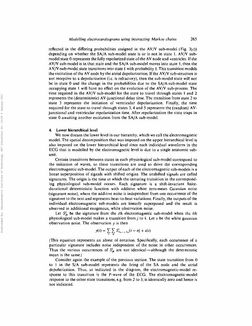
Certain transitions between states in each physiological sub-model correspond to the initiation of waves, so these transitions are used to drive the corresponding electromagnetic sub-model. The output ofeach of the electromagnetic sub-models is a linear superposition of signals with shifted origins. The unshifted signals are called signatures. The origin is the time a t which the initiating transition in the corresponding physiological sub-model occurs. Each signature is a shift-invariant finite- durational deterministic function with additive while zero-mean Gaussian noise (signature noise), where the additive noise is independent from one occurrence of the signature to the next and represents beat-to-beat variations. Finally. the outputs of the individual electromagnetic sub-models are linearly superposed and the result is observed in additional exogenous, white observation noise.

Let Sj, be the signature from the ith electromagnetic sub-model when the ith physiological sub-model makes a transition from j lo k. Let u be the white gaussian observation noise. The observation j8 is then

= 1 ,+,(r - 4 + ~ ( r ) i n

(This equation represents an abuse of notation. Specifically, each occurrence of a particular signature includes noise independent of the noise in other occurrences. Thus the various occurrences of S:, are not identical-although the determinstic mean is the same.)

Consider again the example of the previous section. The state transition from 0 to 1 in the S/A sub-model represents the firing of the SA node and the atrial depolarization. Thus. as indicated in the diagram, the electromagnetic-model response to this transition is the P-wave of the ECG. The electromagnetic-model response to the other state transitions, e.g. from 2 to 3, is identically zero and hence is not indicated.


266 P. C. Doerschuk e l al

I n the AV/V sub-model, the state transition from 2 to 3 represents the initiation of the ventricular depolarization. Hence the electromagnetic-model response to the corresponding transition i s the QRS complex and the T-wave. Here, we are modelling the QRS complex and T-wave as deterministically coupled waveforms-the ST interval duration i s not random. Note that a more complex model of the same type could allow a random coupling. The electromagnetic-model response to the other state transitions i s identically zero.

Several aspects of the electromagnetic model merit comment.

( n ) Note that some anatomic sub-units do not cause waves in the ECG (e.g. the AV node) and therefore the corresponding electromagnetic sub-model does not exist. Similarly, most transitions model the timing between wave and interaction initiations and therefore have no effect on the corresponding electromagnetic sub-model. Thus very few transitions actually contribute to the ECG.

(h) The use of a gaussian white noise to model both beat-to-beat morphology vari:ltions and observation noise i s an obvious oversimplification. Incorpor- ating more complex and realistic models i s straightforward. For example, one could easily use a time series model for each waveform or, by adding states and transitions to a sub-process model, one could introduce additional signature- initating transitions to model dramatically variant morphologies for any particular wave. The observation noise serves the role of modelling all non- non-cardiac contributions to the observed signal, including motion artifact, electromyogram signals, and 60 Hz interference. Again i t i s straightforward to replace the white noise model by a more accurate correlated noise model. As all of these modifications add detail rather than new structure to our models, we have not included them here in order to present the essential elements of our modelling methodology. I t i s worth pointing out, however, that the level of realism needed in such models depends upon the use to which the models are to be put. I f they are used as the basis for signal processing algorithms, model fidelity i s only of indirect importance, as one generally seeks to find the simplest model that leads to a successful algorithm. For example, a white noise model was successfully used in the work of Gustafson et al. (1978. 1981).

( c ) The Markov chain cycle interval need not equal the signature sampling interval. Typically, the Markov chain cycle interval can be taken to be substantially larger than the signature sampling interval, reflecting the dif- ference in time scale between interaction events (which determine the Markov chain cycle interval) and events internal to the anatomic sub-models (which set the signature sampling interval). Because signatures can only be initiated at

Markov chain cycles, unequal intervals appear to imply that signatures cannot be initiated at arbitrary signature samples. However, by using an augmenta- tion technique as in (b), this problem can be overcome. For an example, see the Wenckebach model of $ 6 .

( d ) Given the sampling interval used, the transition probabilities of the sub- models determine not only the sequencing of events but the overall rate at which events occur. Setting these parameters for a specific ECG i s essentially a problen~ in parameter estimation for Markov chains, and a standard algorithm to perform this task would be needed in a complete signal processing system. Moreover, given that ECG behaviour and in particular heart rate may be non-


Modelling elrcrrocurdiogru~ns using inrerucring t\40rl;~rtl cliuins 267

stationary, one may wish to view these transition probabilities as time-varying, or equivalently to incorporate an adaptive parameter estimation algorithm into the signal processing system. Such a system would, of course, also bc needed t o detect changes in rhythm such :IS the onset of tachycardia, much as in the work of Gustafson et al. (1978, 1981).

5. Microscopic model-structural elements In this section we describe the small number ofclemcntary structural elements that

are used in constructing our physiological models. Each of these elements is a piece of a Markov chain. There are two fundamental structural elements, which are essentially elapsed time clocks, out of which three other structural elements are constructed.

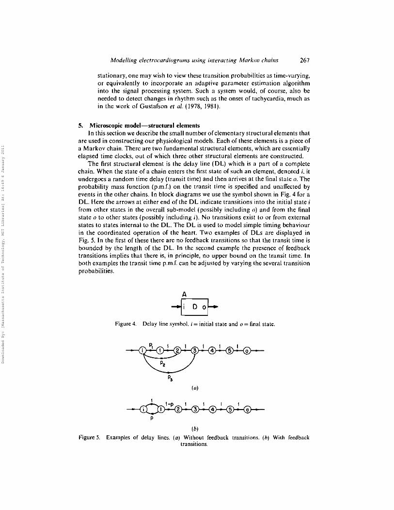
The first structural element is the delay line (DL) which is a part of a complete chain. When the state of a chain enters the first state of such an element, denoted i , i t undergoes a random time delay (transit time) and then arrives a t the final state o. The probability mass function (p.m.f.) on the transit time is specified and unaffected by events in the other chains. In block diagrams we use the symbol shown in Fig. 4 for a DL. Here the arrows at either end of the DL indicate transitions into the initial state i from other states in the overall sub-model (possibly including o) and from the final state o to other states (possibly including i). No transitions exist to or from external states to states internal to the DL. The D L is used t o model simple timing behaviour in the coordinated operation of the heart. Two examples of DLs are displayed in Fig. 5. In the first of these [here are no feedback transitions so that the transit time is bounded by the length of the DL. In the second example the presence of feedback transitions implies that there is, in principle, no upper bound on the transit time. In both examples the transit time p.m.f. can be adjusted by varying the several transition probabilities.

Figure 4. Delay line symbol. i = initial state and o = final state.

( b ) Figure 5. Examples of delay lines. ( a ) Without feedback transitions. ( h ) With feedback

transitions.


268 P. C. Doerschtrk et al.

The second structural element i s the resettable delay line (RDL). This element i s used to model both timing and the resct and stunning phenomena that can occur when a depolarization wave reaches an autorhythmic site. We often use the term delay line as a generic name for both DLs and RDLs. The differences between the RDL and the D L are that there are two different mechanisms for the state to exit an RDL, and an RDL has transition probabilities that are controlled, in a very simple and specific way, by interactions initiated by another sub-process in the overall Markov chain. The possible interactions impinging on a chain containing an RDL are divided into two classes denoted normal and abnormal. Within each class the transition probabilities in the RDL are constant. As long as the interaction i s i n the normal class, the RDL behaves as a DL, transiting from the initial state i toward the final state o. However, when the interaction i s in the abnormal class, a second set of transition probabilities is used for the next transition. The second set of transition probabilities forces the state to leave the RDL and enter a state, external to the RDL, called the resct state and denoted by r.

In block diagrams we use the symbol shown in Fig. 6 for an RDL. Here the dashed arrow and symbol c denote the effect of interactions from other sub-models. The variable c takes on two values: R (for 'reset') i f the current impinging interaction is in the abnormal class and R(for 'not reset') otherwise. An example of an RDL is given in Fig. 7.

The third structural element i s the autorhythmic element which i s capable of sustained cyclic behaviour without external excitation. This element i s constructed from DL(s) and/or RDL(s). The basic idea is to attach the input and output of a D L together, as in Fig. 8. I f a D L is used, this specifies the entire chain. I f an RDL is used,

Figure 6. Resettable delay line symbol. i = input, o = normal output, r = reset output, and c = control input.

Figure 7. Example of a resettable delay line and i t s reset state r


M~IIPIII'II!: c ~ l e c ~ r ~ c i ~ r d i i ~ g r i ~ ~ ~ ~ s using i ~ ~ r r r o c r i ~ ~ g Markou chains 269

Figure 8. Basic autorhythmic element

it is also nccessnry to specify the identity of the reset state (see 5 6.2). The choice of D L vcrsus RDL dcpends on the physiological process being modelled. Typically one or morc transitions in thc autorhythmic clement will initiate ECG signaturcs (corresponding. for example, to the P-wave resulting from the autorhythmic operation of the SA nodc).

Thc fourth clemcnt is the passive transmission line (PTL), constructed from a D L o r an RDL. Wc illustrate the DL case in Fig. 9. A PTL is a connection of a single state, c;dled the resting statc, to the initial state of a DL. The only transition out of the resting state is into thc DL. The probability for this transition. denoted p, depends on the value of the current interaction impinging on the sub-model containing the PTL. The possible v:tlues of this interaction are partitioned into two disjoint sets called the autonomous and non-autonomous sets. When the interaction is in the autonomous set. p=O. That is. the rcsting state is n trapped statc. In the other case (non- autonomous), p z 0. The PTL can be used to model a part of the heart, such as the AV node. that begins dcpolarization only when an external dcpolarization wave excites it. One or more transitions in the PTL may generate signaturcs in the ECG.

The fifth element is the bi-directional refractory transmission line (BDRTL), shown in Fig. 10, which is a complete sub-model and is used to model structures cnpable of supporting conduction in either the antegrade or retrograde direction. All unlabelled transition probabilities in Fig. 10 take on the value 1. The state 0 corresponds to the repolarized resting state of the anatomic substructure. The RDL labelled A ( R ) corresponds to antcgrade (retrograde) conduction. In accordance with these designations. the BDRTL attempts to excite the sub-model(s) corresponding to the adjacent distal (proximal) anatomic sub-structure(s) whenever the BDRTL state occupies state o, (o,), the final state of the antegrade (retrograde) conduction RDL.

r = resting state

Figure 9. Passive transmission line.

Figure 10. Bidirectional refractory transmission line.



RDLs are used here in order to model the possible collision of two depolarization waves, one in the antegrade and one in the retrograde direction. The relationship between the resting state 0 and the RDLs A and R i s a simple generalization of the PTL structural element. The third delay line (F), a DL, corresponds to the refractory period. A non-resettable delay line i s used because, at the level of physiological detail that we are modelling, the duration of the refractory period i s independent of all external events.

The state transition probabilities. p,,,,po,,, and pa., and the RDL state transition probabilities (controlled exclusively through c, and c,) are the only probabilities that depend on the states of other sub-models, that is, on the interactions impinging on the BDRTL. In the absence of external excitations

- po.A = po., = P , , ~ = 0 and c , = c, = R

That is, under these conditions, i f the process was in the resting state, i t remains there until an excitation initiates depolarization. I f the process was in the middle of a depolarization, the depolarization continues in a normal fashion.

l i the BDRTL is excited from the antegrade direction, but not simultaneously from the retrograde direction, then

- po.* = I, po,, = p,,, = 0, c, = R and c. = R

In this case, i f the process was in the resting state, i t immediately exits and begins an antegrade depolarization. I f the process i s in the middle of a retrograde depolarization, the depolarization i s stopped by resetting the RDL. This models the collision of the two depolarization waves. After this point in time the process proceeds through the D L modelling the refractory period.

For the reverse case (i.e. excited from the retrograde direction but not from the antegrade direction), the values are

- po., = I. pO.., = pO.F = 0, C, = R and c, = R

Finally, i f the BDRTL i s simultaneously excited from both the antegrade and retrograde directions, then

PO.F = 1, PO." = PO., = 0. C A = C R = R

Depending on what anatomic sub-structure the BDRTL models, i t may or may not contain transitions which generate a non-zero response in the electromagnetic model. I f the BDRTL does contain such transitions, then there are three basic situations which we illustrate assuming that the BDRTL models the atria which can be excited by the SA node or by retrograde conduction from the AV node. The three situ:~tions in which signatures are generated correspond to the following.

( ( 1 ) Antegrade conduction without a reset (e.g. a normally conducted P-wave from the SA node through the atria).

( h ) Retrograde conduction without a reset (e.g. a retrograde P-wave from the AV node through the atria).

(r) Reset-antegrade or retrograde conduction, corresponding to collisions of two depolarization waves. Such an occurrence generates a so-called fusion depolarization (e.g. a fusion P-wave due to joint SA-nodal and retrograde-AV- junction depolarizations).


mod ell in^ elecrrocardiograms using inrerociing Markou chains 27 1

Though it is not the only possibility, we have used the transition from the resting state to i, or i , to generate the non-reset antegrade and retrograde electromagnetic model responses. For simplicity we have assumed that a fusion depolarization is identical to the response from the earlier of the two depolarization waves. Modifica- tions allowing for a diRerent signature for fusion waves can be easily accommodated.

6. Examples of ECG models The small number of building blocks described in the preceding section can be

used to construct models for any cardiac rhythm. In Doerschuk (1985), we have shown how one can write down models for cardiac arrhythmias involving re-entrant pathways (in which depolarization waves can, in fact, cycle through parts of the heart several times), abnormal atrial-ventricular conduction pathways (such as the so-called WolR-Parkinson-White syndrome), and the presence of ectopic foci (see 5 6.2). In this section we illustrate our methodology by presenting models for three different cardiac conditions: normal rhythm, normal rhythm with ectopic focus premature ventricular contractions, and a type of second degree AV block called Wenckebach. The first two models are specified at the level of the structural elements of the previous section, while the third is described in complete detail.

A simple, graphical notation is helpful in describing the models. Figure 11 illustrates a model made up of four sub-models, denoted by the boxes labelled CO. ..., C3. The directed lines between boxes indicate the existence of an interaction in the indicated direction. Thus, for example, sub-model CO initiates an interaction with sub-model CI . The number of values which the interaction can take on is not specified. The wavy lines terminating in SO, ..., S3 indicate that the sub-model of the originating box contains one or more transitions which initiate a signature whose name is the label at the end of the arrow.

52 s3 $JsO C 2 5'

Figure I I . Illustration of [he block diagram description o f a class of models

6. I . Norn~ol rhgrh~n A block diagram of a model for a prototypical normally conducted rhythm and a

listing of the intersub-model interactions is given in Fig. 12. The heart is divided into four anatomic sub-structures-SA node, atria. AV junction, and ventricles-each of which is modelled by a separate sub-model. Qualitatively, the model behaves in the following manner. The SA-nodal sub-model initiates a depolarization wave. This is the only way in which a depolarization can be initiated in this model. The depolarization then propagates antegrade through the atrial sub-model, producing the P-wave; the AV-junctional sub-model, which makeszerocontribution to the ECC:


and finally the ventricular submodel, producing a QRS-T complex. Because only antegrade conduction is included in the model, sub-model0 is not resettable and sub- models 1 and 2, which would be BDRTLs if retrograde conduction were included, consist instead of DLs.

Sub-model I : Atrial Sub-rtmcturc

Sub-model 2: AV-junctional Sub-rtmcturc

Electromagnetic Model: 0RS.T complex

(4


Modelling elrctrocardiograms using inreracting Markou chains 273

Sut-model 0: Sub-modcl for the SA-nodal Suk tme tu re

lhir sub-model ir autonomous.

Sub-model I : Submodel for the Atrial Sub-structum

Sub-modcl 2: Submodcl for the AV-junctional S u k t r u c l u r r

Sut-model 3: Sub-modcl for the Vrntricular Sub-structure

(4 Figure 12. Model for normal rhythm. ( a ) Sub-model structure. ( b ) Block diagram.

(c) Intersub-model interactions.

6.2. Normal rhythm with ectopic Jocus PVCs

There are numerous autorhythmic sites in the heart, and occasionally, even in a normal heart, one of these sites may successfully initiate a depolarization wave. Such a site is referred to as an ectopic focus or pacemaker. If this focus is located in the ventricles, then the ventricles can contract a short time before the next normal depolarization would have occurred. Such a beat is called a premature ventricular contraction (PVC). PVCs can also arise through a re-entrant pathway mechanism (in this case there is typically a more regular relationship between the timing of the PVC and the previous, normal, QRS complex). I t is certainly possible to model this mechanism using our methodology, but we do not do so here. Because of the anomalous location at which this depolarization starts, the resulting QRS waveform is generally quite

SA nods El

AV junction & R

Venl r i~ le~ PVC

Ectopic

Pacarnoher


P. C. Doerschuk et al

Sub-model 3: Ventricular Substructure


Modelling elecrrocurdiograms esing interacting Murkou chains 275

Sub-model I : Sub-modd for the Atrial Subi t ruc ture

11 if x0 e lo0) and r2 E (o:]

' 10 olhcrwix

Fizure 13. Model lor normal rhvthm with PVCs @enereled bv an eclo~iclocus. la1 Sub-model - - slruclure (hl Hlucl. dlagram. ( 1 . 1 Inlmub-model inleracllon\. These inleraclions arc slmllar to those ollhu nurmal rhblhm model Jcscrthcd in Fly I? Thcrcbre. only !he interactions lor sub-model I are given.

different from a normal beat. Typically the PVC is a more spread-out waverorm as the initiation of the contraction of one ventricle precedes that of the other by a noticeably larger time interval. Furthermore, when a PVC occurs, it is possible for the resulting depolarization wave lo propagate in a retrograde direction, colliding with the normal SA-node-initiated wave o r arriving a t and resetting the SA node.

In order to develop the model for this arrhythmia, described in Fig. 13, we have modified the normal-rhythm model in two ways. First, we have modified the part of the normal-rhythm model which corresponds to the part of the heart which exhibits the abnormal physiology. Therefore we have replaced the ventricular sub-model by a new ventricular sub-model and an ectopic ventricular pacemaker sub-model. In the ventricular model the QRS and the PVC signatures both include their corresponding T-waves. That is, the signature includes the entire depolarization-repolarization cycle. Therefore the inverled T-wave typical of PVCs is directly included here. Second, we have modified, as required, the remaining parts of the normal-rhythm model so that they can interact with [he part modified in the first step. The primary purpose of these modifications is to allow retrograde conduction and resetting of the SA node.

6.3. U'enckebach

Wenckebach is characterized by a multibeat cycle, typically three or four beats long, in which the P-waves are repeated a t constant intervals but the P-R interval grows until, in the final beat of the cycle, the R-wave is dropped. Then the cycle begins again with the P-R interval reset to its initial small value. The increase in the P-R


276 P. C. Docrschuk et al.

interval from brat to beat is usually greatest at the beginning o f the cycle. Physiologically, the cause o f Wenckebach is a defective AV node. Specifically the

AV node is such that i t has a long relative refractory period. A t the beginning o f the multibeat Wenckebach cycle, the AV node i s at rest. The first excitation occurs and is transmitted to the ventricles and the AV node enters its refractory period. Because the refractory period is prolonged, the second excitation from the atria reaches the AV node during its relative refractory period. The impulse is s t i l l able to excite the AV node (although propagation is at a reduced spced) and through i t the ventricles, since thecflective refractory period i s past. However, theearly excitation ofthe AV node has two effects: the following P-R interval and the following refractory period are both prolonged. Thus the third excitation occurs even earlier in the relative refractory period. This lengthening o f the P-R interval and refractory period continues unt i l finally a depolarization wave attempts to excite the AV node during its eKective refractory period and is nor conducted at all. This leads to the dropped R wave and gives the AV node time to complete its refractory period before the next excitation.

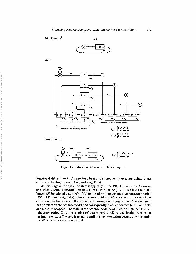
We now describe the behaviour of the AV-nodal sub-model during a Wenckebach cycle (see Figs 14 and 15). Init ial ly the AV node is at rest: x ' = 0. When the AV sub- niodel is excited. the state transitions into the AV, DL. The transit time for this DL is the AV-junctional delay. A transit time from the AV, DL is biased toward shorter valucs than a transit time from any o f the other AV, DLs. Therefore, as desired, this i s the shortest possible AV-junctional delay. After the AV-junctional delay, the AV sub- model attempts to excite the V sub-model: .rl = I. Then the AV sub-model enters the effective refractory period. Note that the effective refractory period contains a transit- time contribution only from the ER, DL and therefore the effective refractory period is short. Following the effective refractory period is the relative refractory period consisting of the tolal time spent in the RR,, RR,, and RR,DLs. I f the next excitation o f thc AV sub-model is sufliciently dclayed. the AV sub-model's state wil l pass through the three RDLs labelled RR,, RR,, and RR, and re-enter the resting state (state 0).

However, that is not what usually occurs. Rather, the refractory period duration is such that the next excitation ofthe AV sub-model generally occurs during the relative refractory period. More specifically, because this first beat of thc cycle had a short AV- junctional delay (using delay line AV,) and a short effective refractory period (avoiding delay lines ER,. ER,. and ER,). the next excitation o f the AV sub-model generally occurs while the AV sub-model's state is in RR,, the final R D L o f the relative refractory period. Therefore. the excitation ofthe AV sub-model forces the AV sub-model's state to transition into the AV, DL, leading to a somewhat longer AV-

Figure 14. Model for Wenckebach. Sub-model structure.


Modelling electrocordiogrr~~~s using inferrrcfi~lg Mirrkou c h n i ~ ~ s 277

AV: I'

I i t .O.O

ow' (0 0fh.rwi..

R i l xO.O Cw. {R oth.r.i,.

Figure 15. Model for Wenckebach. Block diagram.

junctional delay than i n the previous beat and subsequently to a somewhat longer effective refractory period (ER, and ER, DLs).

At this stage o f the cycle the state i s typically i n the RR, DL when the following excitation occurs. Thererore, the state is reset into the AV, DL. This leads to a still longer AV-junctional delay (AV, DL ) followed by a longer effective relractory period (ER,. ER,, and ER, DLs). This continues unt i l the AV state is still in one of the effective-refractory-period D L s when the following excitation occurs. This excitation has no effect on the AV sub-model and consequently i s not conducted to the ventricles and a beat is dropped. The state of the AV sub-model continues through the effective- refractory-period DLs, the relative-refractory-period RDLs, and finally traps in the resting state (state 0) where i t remains unt i l the next excitation occurs, at which point the Wenckebach cycle i s restarted.



The actual Markov chains and signatures are shown in Fig. 16. They were chosen based on a nominal heart rate of 60 beats per minute with a Markov chain cycle period of A s and a signature sampling period of& s. Note the multiple copies of the P-wave signature with one, two, or three leading zeros. These were introduced so that P-waves could begin at any signature sample rather than at only every fourth signature sample ( i s at a Markov chain transition). Similar remarks apply to the V- and T-waves in the V sub-model. Since we are most interested here in illustrating event timing, we have not included beat-to-beat morphology variations (i.e. the signature noise variances have been set to zero).


Modelli~ig elecrrocardiugran~s using interacting Markuu chains 279

( h )

Figure 16. Model for Wenckebach. ( a ) Markov chains. ( h ) Signatures

The Table gives a summary of a few successive Wenckebach periods and Fig. 17 displays the corresponding simulated ECG. Note the lengthening P-R intervals followed by a dropped beat. Note also that the model is not deterministic. For example, sometimes the Wenckebach cycle is four beats long and sometimes it is five.

Time Time since

P-R interval last P wave

dropped 012 0.23 0.24 0.33

dropped 0.16

dropped 018

dropped 009

Model for Wenckebach: simulated P-P and P-R intervals. The simulated ECG from which this interval data were computed is shown in Fig. 17.


280 P. C. Doerschuk et al.


Modell ing electrocardiograms using interacting Markou chains 28 1

Figure 17. Model lor Wenckebach: simulated ECG. The interval data are tabulated i n the Table.

ACKNOWI.EDCMENT We are grateful t o Professor R. G. M a r k for the opportuni ty l o use the M.I.T.

Biomedical Engineering Center's computat ional facililies. The research described in this paper was supported in par t b y the A i r Force Off ice

o f Scientific Research under G ran t AFOSR-82-0258 and the A r m y Research Off ice under Granr DAAL03-86-K-0171. The first named author was supported b y fellowships f r om the Fannie and John He r t z Foundat ion and the M.D.-Ph.D. Program a t Harvard Univers i ty (funded in pa r t b y the Publ ic Heal th Service, Na t i ona l Research Award 2 T 32 GM07753-06 f r om the Na t i ona l lnst i tu te o f General Med ica l Science).

REFERENCES BoR~usoN. P. 0.. PAHLM. 0.. SORKMO. L.. and NYCARIX. M.-E.. 1982, Adaptive QRS detection

based on maximum rr posruiori estimation. I.E.E.E. Truns. Bio-nzed E~gng, 29, 341 CKICLODA. Gh.. Digital analysis of RR intervals for identification of cardiac arrhythmias.

Section 11. Irzr. J. Biol-hid. Comptdr.. 14. 155. C ~ H N . R. L.. RUSII. S., and L~~PISCHKIN. E.. 1982.Theoretical analyses and computer simulation

o f ECG ventricular gradient and recovery waveforms. I.E.E.E. Trurts. Bio-wed Eupg. 29, 413.

Cox, J. R., Jr, NOLLI:, F. M.. and ARTHUR, F. M., 1972, Digital analysis of the electroencephalo- gram. the blood pressure wave, and the electrocardiogram. Proc. I,ur,t elecr, elecrrort. Engrs. 60. 1137.

DOERSCHUK, P C.. 1985, A Markov chain approach to electrocardiogram modelling and analysis. Ph.D, thesis. Department of Electrical Engineering and Coniputer Science. Massachusetts lnstitute of Technology, Cambridge. Massachuselts.

Dosnsc~ur;. P C.. TEKKBY. R. R., and WILLSKY. A. S., 1990. Event-based estimalion o f interacting Markov chains with applications to electrocardiogram analysis, lnr. J. Swents Sci.. 21. 285-304.

R~LIIMAN. C. L.. and HURELRANR, M.. 1977. Cardiovascular monitoring i n the coronary care unit, bled. Itlrrrun~., 11, 288.

GERSCH, W.. EDDY, D. M.. and DONG, E.. Jr.. 1970. Cardiac arrhythmia classification: a heart- beat interval-Markov chain approach. Contpur. Bio-rrrd. Res., 4, 385.

GERSCH. W.. LILLY. P., and Dose, E., Jr., 1975, PVC detection by the heart-beat interval data- Markov chain approach. Con~p~~r . Bio-wed. Res.. 8. 370.


G r s ~ ~ o w r r z , D. B., 1979, Magnetocardiography-an overview. I .E.E.E. Trms. Bio-md. Engng, 26, 497.

G U S T A ~ N , D. E., WILLSKY, A. S.. WANG. J.-Y., LANCAST~R. M. C.. and TRlliRWASSER, J. H., 1978, ECG/VCG rhythm diagnosis usingstatistical signal analysis. Part I: identification of persistent rhythms. Part 11: identification of transient rhythms. I .E.E.E. Tram. Bio- med. Engng. 25, 344.

GUSTAFSON. D. E.. WANG. I.-Y., and WILISKY, A. S., 1981, Cardiac rhythm interpretation using statistical P and R wave analysis. Fronriers ((Enginccring in Ileal111 Care, edited by B. A. Cohen (New York: I.E.E.E.), pp. 267-272.

HAYWOOD. L. J.. MURTI~Y. V. K.. HARVEY. G. A,, and SALTZRI~RG, S., 1970. On-line real time computer algorithm for monitoring the ECG waveform. Compur. Bio-mud. Rl's.. 3, 15.

Hnts~ov, H. R.. ASTARUJIAN. G. B., and NACIIEV, C. H., 1971, An algorithm for the recognition of heart rare disturbances. Med. hiol. Engng, 9, 221.

LEBLANC. A. R.. and RORERGE, E A,, 1973, Present state of arrythmia analysis by computer. Canadian hfedical Assoc. J., 108, 1239.

McFlili, R., and BAULI. G. M., 1972, Research i n electrocardiology and magnetocardiology. Proc. Iasr. Elect. Elecrron. Engrs. 60, 290.

MILI.I:R, W. T , and GI:SI~I.OWITZ, D. B., 1978, Simulation studies o f elcctrocardiopram, part I: normal heart. Part 2: ischemia and infarction. Circul. Res., 43, 301.

Moli, G. K., and MENIXZ, C., 1966, Simulation o f impulse propagation i n cardiac tissue. Ann. N.Y Acod. Sci.. 128, 766.

MuRTHY, I. S. N., RANGARAJ, M. R., UINPA, K . J.. und GOYAL, A. K., 1979. Homomorphic analysis and modelling o f ECG signals. I .E .E.E. Truns. Bio-med Engng. 26, 330.

O~ l v l i n . G. C., RIPLEY, K . L., MILLER. J. P.. and MARTIN. T. F., 1977, A critical review of computer arrythmia detection. G m p r r c r Electrocordiogrnp1,p: Presrnr Srurus and Criteria, edited by L. Prody (Mount Kisco, N.Y.: Futura Press), pp. 319-360.

P ~ o w n , R.. 1979, Fundamentals of electrical processes i n the electrophysiology of the heart. Advances in Cardior:ascular Phpics. Vol. I : Tl~enrcricrrl Foundalions of Cardivua.scular Processes, edited by D. N. Ghista. E. Van Vollenhoven, W-J. Yang and H. Reul (Basel: S. Karger), pp. 1-28.

RICHARIISON, J. M., HAYWOOD. L. J., MURTHY. V. K.. and KALADA. R. E., 1971, A decision theorctic approach to the detection of ECG abnormalities. Part 11: approximate treatment o f the detection of ventricular extrasystoles. Morh. Biosci.. 12, 97.

R o s a ~ n l ~ G , R. M.. C l t ~ o . C. H.. and Aseorr, J.. 1972, A new mathematical model ofelectrical cardiac activity. Marh. Biosci., 14, 367.

SHAII. P. M., ARNOLIX J. M., HARI~RI~RN, N. A., BLISS, D. T., MCCLI:LLANU. K . M., and CI.ARKI?, W 0.. 1977. Automatic real time arrythmia monitoring in the intensive coronary-care unit. Am. J. Curd., 39, 701

SMITII. J. M., 1982, Finite element model of ventricular dysrhythmias. M.S. thesis. Department of Electrical Engineering and Computer Science, Massachusetts Institute o f Tech- nology. Cambridge, Massachusetts.

SORNMO. L.. B0RJr:ssoN. P. 0.. NYGARUS, M.-E., and PAHLM, O., 1981, A method for evaluation of QRS shape features using a mathematical model for the ECG. I .E .E.E. Trans. Bio- med. EIIKIIZ. 28, 71 3.

THIRY, P. S., and &SENDERG. R. M.. 1974. On electrophysiological activity o l thc normal heart. J . Frunh.lin Insl.. 297, 377.

THIRY, P. S., RO~ENRI:RG, R. M.. snd A e ~ o r r , J. A,. 1975, A mechanism for the electrocardiogram response to left ventricular hypertrophy and acute ischemia. Circul. Res., 36.92.

T t i o ~ n s , L. J., Jr.. CLARK, K . W., MEAD; C. N.. RIPLI~Y. K. L., SPI:NNI:R, B. F.,and OLIV~R, G. C., Jr., 1979, Automated cardiac dysrhythmia analysis. Pmc. lnsrn elect. elccrron. Engrs, 57, 1322.

Tnl r r , J. H., 1979, Theory o f the magnetocardiogram i n Advances in Cnrdiucascular Physics. b l . I : Tbeorericol Fou~~dor~ons ~fCardioua.scular Processes. Edited by D. N. Ghista, E. Van Vollenhoven, W:J. Yang and H. Reul (Basel: S. Karger), pp. 29-46.

Tsut. E. T., and WONG. E.. 1975. Sequential approach to heart-beat rhythm classification. I .E .E.E. Trans. InJ: Tlreorg, 21, 596.


Model l ing elecrrocardiograms using interacring Murkou chains 283

UlJaN, C. 1. H., DE WEERD, J. P. C., and VEIDRIY. A. J. H., 1979, Accuracy of QRS detection in relation to rhe analvsis o f hieh lreauencv comoonents i n the eleclrocardioerarn. Med. - . . - hid. Engng Carnpul., 17, 492.

VINKE, R. V. H., ARNTZENIUS, A. C., HUISMAN, P. H., KULRERTUS. H. E.. RITSEMA VAN ECK, H. J., SCHIPPERHEIJN. J J., and SlMmNs, M. L., 1977. Evaluation of a computer model of ventricular excitation. Proc. Cornpuf. Cardiologv. 4, 605.

WHITE. C. C. . 1976, Note on a Markov chain approach to cardiac-arrythmia classification. Compel. Bio-med. Res., 9, 503.

WIKSWO. I . P. Jr.. MALMIVUO, J. A. V., BARRY. W H.. LEIER, M. C.,and FAIRRANK. W. M., 1979, The theory and application of magnetocardiography, Advunccs in Cardiouascular Pltesics. Vol. 2; Cordioerums: Tl~eons and A~dical ion. edited bv D. N. Ghista. E. Van ~d lenhoven, W:J. ~ a n g and H. ~ e u l (Bas& S. ~a rge r ) , pp. 1-67,

ZLCKJF. M., ROSIINBERG. R. M.. and ARROIT. J., 1973, A computer model for atriovenlricular blocks. Morb. Biosci.. 18, 87.


Documents

International Journal of Systems Science Modelling