Statistical regression modelling of glass properties – a ...glassproperties.com/principle/Statistics_Glass_2007.pdf · Glass Technology: European Journal of Glass Science and Technology

Glass Technology: European Journal of Glass Science and Technology Part A Volume 50 Number 1 February 2009 �

IntroductionIn glass research and technology, it is often neces-sary to reduce the costs of raw materials, to improve specific properties, or to design a glass composition for new applications. To meet these needs, the use of personal experience and published scientific literature is advantageous. In recent years, the crea-tion of large glass property databases has facilitated systematic glass property modelling and property measurement evaluation. It is no longer required to search worldwide for numerous individual publica-tions regarding specific properties. The commercially available systems SciGlass(1) and Interglad(2) combine hundreds of thousands of experimental findings from the majority of glass research papers from over a cen-tury, including the associated references. In addition, SciGlass gives details about measurement methods. Furthermore, predictions are possible in SciGlass through models published previously, and Interglad includes a predictive linear regression feature.

Despite the recent progress, there are several shortcomings in these commercial tools:(1) Numerous experimental data from various inves-

tigators differ significantly, even within simple glass systems and for well investigated properties (see Figure 8 in the discussion of future work).

(2) Many predictive glass property models exist in the literature, and it is sometimes difficult to decide which model is the most appropriate.

(3) Industrial glasses have complex compositions, and it is not always possible to predict properties through commonly used linear property–compo-sition relations.

(4) Some of the published models are based on sci-entific principles or derived assumptions about the details of chemical bonding within a glass. Therefore, experiments need to be interpreted (that lead to those scientific principles or to those derived assumptions about the details of chemi-cal bonding within a glass) before some models can be established. This can be a source of error based on the accuracy of this interpretation.

(5) Some models consider the experimental find-ings of a few or only one single investigator, i.e. systematic errors of a few investigators easily can lead to incorrect conclusions. Systematic errors of whole data series are known in glass science as described below in Table 2, and referred to at the end of Step 7 of the statistical analysis (outlier analysis, data leverage).

(6) The prediction errors for models based on one investigator reflect the measurement precision in her/his laboratory, but it is not possible to conclude how such prediction errors will relate to those based on data from other laboratories.

In this work, an attempt is made to overcome these problems above for practical application in glass technology. The goal is a method that features quan-titative prediction accuracy and simplicity. Therefore, it is not a requirement to have an expert knowledge of all details of the nature of glass, the published modelling techniques, or advanced mathematical procedures. It is also not necessary to acquire expen-sive software (besides common spreadsheet software like Excel) or a high performance computer. However, it is strongly advised to rely on experience about the subject matter, and, if possible, on dedicated software that can perform some of the procedures described in this tutorial automatically.

Statistical regression modelling of glass properties – a tutorialAlexander FluegelPacific Northwest National Laboratory, Richland, WA 99352, USA

Manuscript received 5 August 2005Revised version received 14 July 2006Accepted 28 July 2006

Known statistical analysis methods are described in detail with the aim of developing a new and more accurate modelling approach for glass properties. It is shown that the combined analysis of historic and current data from, for example, the SciGlass and Interglad databases, often provides the basis for making property predictions that are more reliable than the raw data itself or a few test measurements. Targeted glass research and process modelling can be facilitated by the approach outlined.

Now at xxxxxxxx. Email XXXXXXXXXX@xxxx

Glass Technol.: Eur. J. Glass Sci. Technol. A, February 2009, 50 (1), xxx–yyy

� Glass Technology: European Journal of Glass Science and Technology Part A Volume 50 Number 1 February 2009

High accuracy can be obtained by using (1) a large number of experimental findings from the commercial SciGlass and Interglad databases and (2) well established statistical analysis techniques. The statistical approach outlined here is not original in general, as numerous publications can be consulted about the topic,(3–9) written over two centuries. In the current work, the statistical method largely follows general techniques that are applied successfully, for example by Harold S Haller & Company(10) in busi-ness consulting, by Bechtel Hanford Inc. for nuclear waste vitrification,(11) and for modelling of solar con-trol glasses.(12) Statistical analysis is also firmly estab-lished in numerous areas in quality control, economy, biology, sociology, politics, etc., to mention just a few applications. The range of applications underlines the basic character of statistical analysis that has been ignored for too long in glass science.

Statistical analysis in glass science and technology

Ernst Abbe, Otto Schott, and A. Winkelmann initiated methodical studies of glass properties in the 19th century, creating the basis of modern glass science in Jena, Germany. They considerably improved the use of glasses for special applications, e.g. for optics, thermometers, and as a thermal shock resistant mate-rial. Winkelmann & Schott published the first model that allowed the prediction of glass properties based on the chemical composition, using the additivity principle,(13,14) i.e. multiple regression using linear functions. This principle is based on the assumption that the relation between the glass composition and a specific property is linearly related for all component concentrations. In this case all of the component influences can be summed as follows

Property i i= +=Âb b0

1C

i

n (1)

where β0 in Equation (1) is the model intercept, n is the total number of significant glass components exclud-ing the main component (usually silica), the i values are the individual numbers of the significant glass components, the βi values are the component-specific coefficients, and the Ci values are the concentrations of the glass components (also called model factors or independent variables).

The additivity principle allows for very precise and accurate predictions within limited concentration ranges,(12,13,15–24) that cannot be reached by structural,(25–

29) thermodynamic,(30–53) or molecular dynamic(54–56) modelling approaches. Because of the simplicity of the technique, the ease of interpretation, and good prediction results within specified limits, Equation (1) is most widely used for glass property modelling. The additivity principle cannot however be applied

for modelling glass properties over wide concentration ranges because of component interactions.

The glass models summarised above are not dif-ferent in principle. Procedures expressed through equations based on specific variables are always established for property–composition relationships. The variables and equations vary, however, and sometimes the variables are derived beforehand from basic principles (“ab initio”) which are in turn based on other (basic) observations such as the atomic mass, bonding distance, bond strength, electron af-finity, stochiometry, or elemental charge. Therefore, all models are empirical by nature, while in ab initio models the empirical character is hidden within fundamental laws about property relations. Often, property modelling derived from other observed properties is less reliable (but scientifically more interesting) than direct modelling of observed prop-erties. Because the nature of glass is not sufficiently well understood, few models exist where different kinds of properties can be mutually derived from each other, e.g. thermodynamic and rheological properties, even though rheological properties can be determined from thermodynamic properties. The final goal is to understand the meaning of all the variables and relationships in glass models in detail. In the current work, it is suggested that the problem should be approached stepwise, i.e. an empirical start is made using simple linear and polynomial relations between the glass composition and observed properties. Once all relevant phenomena have been recognised and organised by means of basic statistical analysis, the step from observation to interpretation can be performed with much higher confidence than without statistical analysis.

In the following paragraphs, simple statistical analysis will be developed for glass property model-ling as the most basic tool of data organisation and interpretation.

Single linear regression using linear functions

Property=β0+β1C (2)

The terms β0 and β1 in Equation (2) are regression coefficients and C is the regression factor or independent variable (glass component concentration). Equation (2) can be used for glass property modelling in binary systems within narrow concentration limits.

Single linear regression using polynomial functions

Property=β0+β1C+β2C2+β3C3+… (3)

Equation (3) can be used for modelling in binary glass systems within wide concentration ranges as long as sufficient data exist and sharp property extrema(57,58)

A. Fluegel StAtiSticAl regreSSion modelling oF glASS propertieS – A tutoriAl


caused by significant crystallisation, phase separa-tion, or other effects do not occur.

Even though nonlinear polynomial functions are used in Equations (3), (6), and (7), those equations are still linear in the coefficients and they are solved using linear regression. All coefficients of the higher order terms in Equations (3), (6), and (7) are determined in exactly the same way (through Equation (12), see below) as the first order additive terms in Equations (1), (2), (4), and (5). An example for non linear regres-sion is described below.

Multiple linear regression using linear functions

Property=β0+β1C1+β2C2+β3C3+… (4)

Equation (4) is identical to Equation (1). It may be applied for glass property modelling in multicom-ponent systems within narrow concentration ranges under exclusion of sharp property extrema such as caused by crystallisation, phase separation, and other effects. Component interactions are not considered in this model form.

It needs to be mentioned that the intercept in Equa-tions (1) to (4) may be eliminated if the main glass component silica (SiO2) is included in the equation. For example, in the binary system SiO2–Na2O Equa-tion (2) may be modified as follows

Property=β0+β1C(Na2O)=β2C(SiO2)+β3C(Na2O)+… (5)

[Author: please check this equation, not sure about the second "="]The approach using an intercept is called “slack variable” (SV) technique and the approach without results in a “canonical” or “Scheffé” type model.(59) Both approaches are very similar statistically; how-ever, the canonical form of the model is expected to produce slightly more accurate predictions if the main component concentration varies significantly or even approaches zero. The slack variable technique will be the main focus of this study because it can be straightforwardly applied to common binary systems such as SiO2–Na2O using squared and cubic terms for Na2O that are not allowed in the canonical technique, as discussed in the following section. Most com-mercial glasses contain silica as the main component (about 40 to 85 mol%) that can be excluded, and slack variable modelling results can be interpreted easily: a specific coefficient shows the property variation caused by the exchange of 1% of the considered com-ponent for silica. The multiple regression coefficients obtained with the slack variable (SV) technique are similar to the values commonly depicted in “spider graphs”.(16,17) Except for the constant term, β0, the SV coefficients must be interpreted as resulting from interactions with the excluded main component silica (Ref. 6, p15–18 and 333–343); while in a canonical

model the coefficients show the extrapolated proper-ties of the related pure components in the (theoretical) vitreous state. All equations described in this work can be applied for the SV and canonical modelling approaches as described below.

Multiple linear regression using polynomial functions

Property=β0+β1C1+β2C2+β3C3+…+β4C12+β5C2

2+β6C32+…

+β7C1C2+β8C2C3+…+β9C13+…β10C1

2C2+β11C12C3+… (6)

Equation (6) is analogous to Equations (2) to (5). The exact form of Equation (6) for the SV regression model using polynomial functions of the second order

Property i i i i ik i k= + + +ÊËÁ

ˆ¯̃= +=

ÂÂb b b b02

11C C C C

k i

n

i

n (7)

where β0 is the intercept, βi are the single component coefficients and the coefficients of squared influ-ences, and βik are the coefficients of two component interactions. The variable n in Equation (7) is the total number of the significant glass components excluding silica; j and k are the indices of the significant glass components, and the C-values are the component con-centrations (excluding silica) in mol or mass fraction or percent (preferably mol fraction or percent). Equation (7) or its canonical variation may be used for glass property modelling in multicomponent systems over wide concentration ranges.(11,60–66) Sudden property changes, such as changes caused by crystallisation and/or phase separation, are difficult to describe with multiple regression using polynomial functions;(58) therefore, advanced nonlinear functions should be applied in these cases. For example, only within very limited concentration ranges can glass liquidus tem-peratures be modelled with linear regression using polynomial functions,(22,23,67–69) as long as the primary crystal phase is constant or has little influence.

If all high order terms are examined in a second order canonical model, then only cross product terms (CiCk), and no squared terms (Ci

2), are allowed to avoid over-parameterisation caused by the mixture constraint C1+C2+C3+…+Cn=100%. However, if only some of the second order terms are populated, then both cross product and squared terms can appear in a “reduced” model.(70)

Multiple nonlinear regression using advanced functions

It is possible to introduce advanced functions into Equation (7), or the structure of the equation may be changed completely. Chemical equilibria between spe-cies in glass may be considered.(36,43,44,71) The exact cal-culation of chemical equilibria based on equilibrium constants and total concentrations requires the solu-



tion of high order polynomials, e.g. a second order polynomial for a two component mixture including one interaction,(64) or a fifth order polynomial for a three component mixture including all three pos-sible two component interactions. Multicomponent mixtures can be calculated numerically using a high performance workstation.

A widely applied nonlinear approach is neural network regression:(72) logistic activation functions such as ex/(1+ex) or tanh(x) are used as “neurons” that make graduated yes/no “decisions” according to the input signal. Several neurons are connected following specified rules, partially comparable to neural networks in biology. The connections between the neurons are weighted, i.e. the signal is amplified or reduced. The “weights” are the fitting coefficients that are optimised using neural network regression. Dreyfus et al(58) demonstrate the application of neural network regression for glass property modelling. They show that neural network regression is ad-vantageous compared to multiple regression using polynomial functions if the glass property does not change gradually with the chemical composition, but sharp property extrema do occur such as liquidus surfaces. Polynomial functions do not fit the sharp extrema well that may appear in glasses because of crystallisation or phase separation.

For building a neural network, component inter-actions have to be assumed and the total number of adjustable weights in neural networks regression needs to be always larger than two times the number of significant glass components. Therefore, neural network regression requires a very high number of data points within an experimental region where interactions can be investigated. Typically multiple training sets are used to “teach” the neural network prior to application to prediction. Each training set will require at least as many data points as adjustable weights used by the network to predict response.

Advanced procedures for obtaining optimal regression fits

During regression analysis, often the “ordinary least squares” (OLS) technique is applied to derive coefficients for each factor, this technique minimises the sum of squares of the differences between the observed and calculated glass properties (unexplained errors, residuals). It is assumed that all unexplained errors are normally distributed with a mean of zero and with no mutual correlation of errors. Significant outliers that influence the result should not exist. If those conditions do not apply, then advanced pro-cedures for obtaining optimal regression fits can be used, e.g. robust regression.(73,74)

For glass property modelling, it is commonly not required to evaluate further fitting methods besides

OLS. In addition, the leverage analysis described below in the section “Step 7: Outlier analysis, data leverage” allows the detection and handling of out-liers that influence the result.

Limits of regression analysis for glass property prediction

In principle, regression analysis can be applied to glass property data so long as a systematic relation exists between the experimental conditions such as concentrations and the resulting properties. How-ever, even though regression analysis can be used in almost all cases, it may be used incorrectly. The most important issue is the possibility of sharp ex-trema in glass properties. Besides crystallisation and phase separation effects, sharp extrema may occur in glasses with a network former content higher than 85 to 90 mol%. For example, the Littleton softening point of 100% pure silica glass may be estimated as 1666±50°C from 54 datapoints in SciGlass.(1) If as little as 0·06 mol% sodium oxide is introduced, then the Littleton softening point decreases dramatically to 1280°C according to Leko.(57) In addition to high silica glasses, sharp property extrema may also be expected for glasses with high concentrations of B2O3 (based on modelling studies of the author; see also publications by Appen and Gan Fuxi), P2O5, and GeO2 or if extreme compositions have to be quenched fast to prevent crystallisation (e.g. 50 mol% Na2O plus 50 mol% SiO2). Sharp property extrema also appear to exist in alkali aluminosilicate glasses with high Al2O3 concentrations,(75,76) especially at low temperatures if the molar ratio Al/Na is approximately 1 to 1·2.

If sharp property extrema occur that cannot be described through the inverse of concentrations, then advanced regression techniques must be applied. Equation (7) must be modified substantially, or the model application range must be narrowed.(22,23,67–69)

Many property data in glass related scientific publications were not obtained using optimal experi-mental designs, and most papers were not published in mutual cooperation. This fact leads to sometimes strong correlations among the model variables (see below, section “Step 4: Correlation analysis”), i.e. vari-ables partly depend on each other. Strong correlations can be excluded through the procedure described below, but even weaker correlations always need to be considered during interpretation of the model results (see below).

For models based on simple assumptions, advanced interpretations are hardly possible. For example, it is completely out of the question to derive atomic radii, chemical equilibrium constants, or properties of pure silica from polynomial models based on a few soda–lime–silica glasses. Model appli-cation limits must be followed as described below in



the section “Step 9: Model application”. Sometimes, interesting interpretations can be derived from mul-tiple regression models, for example about the mixed alkali effect and the influence of batch materials on the glass viscosity.(77) Advanced regression models may allow further interpretation.

Selection of the appropriate regression technique

In general, regression analysis should be used accord-ing to the available data. Within narrow concentration limits, the linear additivity approach is most appro-priate whereas wider concentration limits require polynomial functions. If property extrema appear (e.g. through crystallisation, phase separation, or in glasses with a network former content higher than 90 mol%) that cannot be described via the inverse of concentrations, then advanced regression techniques should be applied. The transition between the re-gression approaches is gradual. Most important for deciding which technique should be used is the study of the linear correlation matrix (see below, Step 4: Cor-relation analysis) of the available concentration data as well as the analysis of binary, ternary, and other related systems for evaluating the crystallisation and phase separation tendency, the property extrema, and general property trends.(78) In addition, all the mod-elling techniques not based on regression analysis that are summarised in the introduction should be evaluated according to scientific experience.

Regarding commercial silicate and borosilicate glasses, it is recommended in this paper, for practi-cal reasons, to initially apply the additive multiple regression technique according to Equation (1) or to introduce selected higher order terms according to Equation (7). It will be explained below, beginning with the section “Step 3: Selection of the model type; establishment of all possible variables”, how the higher order terms are selected.

Analysis procedure using common spreadsheet software

Step 1: Selection of the source dataThe glass property of interest must be defined. According to general previous experience a glass composition region should be selected. The compo-sitional region does not need to be very specific at first. It is helpful to extract all available values from the databases SciGlass(1) and Interglad,(2) and other data sources. If the desired property was never or only seldom investigated in the compositional area of interest, then new experiments should be designed and performed.

The uniformity of the selected source data (the frequency of outstanding or special glass composi-tions within the source data) can be evaluated with

the leverage analysis described below (h-value). In many cases, outstanding glass compositions can be recognised empirically by sight without further calculations. If possible, outstanding glass composi-tions should be excluded from the model, or it should be verified that the reported properties are correct through repeated experiments.

All concentration values must be converted to either mol%, wt%, or concentration ratios, where mol% may be preferred, especially over relatively wide concentration ranges. Models based on mol% can be interpreted more easily, for example regarding the mixed alkali effect.(77)

Step 2: Calculation of property fixpoints and error normalisation

For obtaining optimal results, it is beneficial to stay as close to the original data as possible. For example, it is better to fit original viscosity data than the derived constants of the Vogel–Fulcher–Tammann equation, as demonstrated by Fluegel and co-workers.(20,77) Furthermore, properties should be preferred that require as limited a number of measurements as possible to reduce error propagation. For instance, glass corrosion rates may be expressed in mm/day, which requires measurement of only the corrosion layer thickness and time. Glass corrosion rates may also be expressed in g/m2day, where in addition to the corrosion layer thickness and time, the glass density also has to be determined. Three measurements are likely to contribute more error to the desired property than two measurements.

A property fixpoint must be selected for all glasses that need to be analysed. If possible, not only the directly given data may be considered, but also safe interpolations should be taken into account; e.g. if a property is known at 800°C, 900°C, and 1100°C, it is in many cases possible to estimate for 1000°C.

For selecting an appropriate scale for the property fixpoint, it is required initially to estimate the overall error distribution. For example, it can be assumed that all density measurements expressed in g/cm3 have a similar error, independent from the absolute value; i.e. a glass density of 2·5 g/cm3 can be measured with approximately the same precision as a glass density of 5 g/cm3. This is not the case for all properties. For example, a glass viscosity measurement at 100 Poise is related to a much lower absolute error than a viscosity measurement at 1013 Poise. However, the relative errors of all viscosity measurements are closer to a constant, i.e. a constant percentage of the absolute value. Therefore, viscosities are commonly expressed on a logarithmic scale, also called data transformation, which normalises relative errors to absolute errors. In Figure 1 the influence of logarithmic transformation on the observed property is demonstrated.



In glass technology, it is recommended either to model the desired glass properties directly without data transformation or to determine the logarithm (natural or decadic) of the property.

Figure 2 illustrates the systematic approach con-cerning instances when logarithmic transformation for error normalisation should be considered; after modelling a plot of the observed property values versus the differences of observed and calculated property values (residuals) shows increasing residual variance with increasing property value. In other words if large observed property values appear ap-parently as outliers as seen in Figure 2 logarithmic transformation for error normalisation is advised.

Besides the logarithmic approach, further error normalisation techniques are not common for glass property modelling. In a few cases reciprocal nor-malisation is possible.

Step 3: Selection of the model type; establishment of all possible variables

It is proposed to select the model type from Equa-tion (1) for narrow concentration ranges if only few

experimental data are available, or Equation (7) otherwise. In glass technology, it is seldom required to apply more advanced functions.

For facilitating practical application, a statistical analysis example will be demonstrated below. The ex-ample is entirely artificial. Ten experiments, produced in two laboratories, will be analysed with Equation (1) within a five component glass system. Table 1 gives the concentrations of the five components A, B, C, D, and E, the related property, and the laboratory designation. It may be known to the statistical analyst that in Laboratory 1 a new measurement method was attempted that is assumed to be as sensitive to glass composition changes as the well established method used in Laboratory 2, but also that is assumed to not give the correct absolute property value.

If component interactions need be analysed, sev-eral columns need to be added to Table 1 that contain the concentration products of interest, such as B.C, B.D, and B.E as well as squared terms, e.g. B2. In this example, nonlinear terms will not be considered.

If the glass compositions to be analysed contain elements in various oxidation states, every oxidation state should be introduced as a separate variable. Often


Figure 1. Non transformed and transformed data

Figure 2. Logarithmic error trend


however, the exact ratios of the oxidation states of an element in glass are unknown. Then, it is only pos-sible to consider the sum of all oxidation states as one variable. For example, in most cases, the exact ratio of Fe(III)/Fe(II) in glass is not measured, and Fe(III) plus Fe (II) must be taken as a single variable (considering two Fe ions in Fe2O3 and one Fe ion in FeO).

If glass component interactions are well known from the literature, e.g. mixed alkali effects or boron oxide anomalies, it should be confirmed that cor-responding interaction variables are established. Ex-amples of this are the concentration products Na2O.K2O and Na2O.B2O3. All possible interaction variables also may be added, in case some of them turn out to have a significant influence. (Variable deselection will be described later based on correlation analysis and factor significance.)

If reasonable, further variables could be created, such as the inverse of concentrations to account for extreme end term properties, concentration ratios, etc, Ref. 6, p 286. It is not beneficial in many cases for common glasses with C(SiO2)=40 to 85 mol% to consider the mentioned unusual variables because most of them can be reduced to linear influences of the glass components or component products within the concentration ranges studied. Unusual or complicated variables should be used only if they reduce the number of variables significantly, improve the model fit, or if there are other reasons to evaluate their impacts.

In cases where various data series are combined, as seen in the example given in Table 1, (Labora-tories A and B), it is possible that so-called “block effects” occur. For example, it might happen that experimental results produced in one laboratory (or study) are systematically different from those produced in another laboratory (or study). This could be caused by a different calibration procedure or by different expertise. It also might be possible that a newly introduced measurement technique results in systematically different findings than previously established techniques. In the begin-ning of the statistical analysis procedure, it is best to assume that block effects might be present in all cases; even so, it could turn out later that most of

them do not exist in fact. This means the creation of “categorical” or “dummy” variables(3,4,7) in Equations (1) or (7). In glass property modelling, block effects should only be introduced into the calculation with the forward selection approach (see below in section “Step 6: Calculation of the model standard error, the coefficient errors and significance”). All block effects must be excluded from the model initially and only considered if significant and reasonable.

Property observed=Equation (7)+β(offset) (8)

Property observed=Equation (7) +Property observed×β(trend) (9)

As a result, it would be required to add further columns to the regression dataset in Table 1, accord-ing to the number of data series examined. Following Equation (8), these columns would contain the value of “1” for each experiment within the series, and the value of “0” for each experiment of other series (see Table 2). Following Equation (9), the “1” would be replaced by the property value itself.

If only two data series are examined and block effects occur, it is not possible to decide which one of the data series should be given the block variable (see example in Ref. 20). Further knowledge may help one to decide.

Equation (9) should be applied with caution, and only if measurement trends are reasonable based on knowledge of the subject matter and if several other data series without a measurement trend including a high number of experiments exist. If Equation (9) is used for most experiments, the result would be a perfect fit with a trend coefficient of 1, even if all the experimental findings were seriously incorrect. A trend according to Equation (9) can be converted to an offset according to Equation (8) through logarith-mic normalisation described in the previous section “Step 2: Calculation of property fixpoints and error normalisation”.

Step 4: Correlation analysis

When using multiple regression, it is always impor-tant to evaluate possible factor correlations at the beginning. The linear correlation matrix is made up


Table 1. Example glass composition–property data for statistical analysis Compositions in % Property A B C D E Laboratory 1 88 1 0 1 10 69·4 78 3 3 8 8 15·8 73 5 7 9 6 18·6 76 7 8 5 4 30·8 88 9 0 3 0 25·7Laboratory 2 75 2 10 4 9 71·1 77 4 7 5 7 62·5 84 6 1 4 5 53·3 83 8 2 5 2 64·1 74 10 9 7 0 93·4

Table 2. Analysis of block effectsSeries Chemical Composition Offset Variable PropertyLaboratory A … … … 1 P1Laboratory A … … … 1 P2Laboratory A … … … 1 P3Laboratory A … … … 1 P4Laboratory A … … … 1 P5Laboratory B … … … 0 P6Laboratory B … … … 0 P7Laboratory B … … … 0 P8Laboratory B … … … 0 P9… … … … 0 …


of the simple, or two way, correlation coefficients. They are denoted by the letter “r” and have a range of −1<r<+1 (Pearson’s “r”). The correlation coefficient for two factors (variables) is a measurement of the linear relationship between the two factors. If r is close to 1 then a plot of the two factors against one another would look like a straight line with positive slope. If r is close to −1 then the plot of the two fac-tors against one another would look like a straight line with a negative slope. If r is close to zero then a plot of the two factors would have no discernible linear trend.

For selecting the appropriate model variables, correlations between changes in the components’ concentrations and/or their interactions (concentra-tion cross products) have to be considered if the data were not collected using a statistical design that is “orthogonal” (not correlated) for all of the factors of interest. If the absolute value of r is larger than approximately 0·5 to 0·6, then the influences of the two considered factors are “partially correlated” (i.e. linked but not completely aliased) and may be dif-ficult to separate. If the absolute value of r is larger than approximately 0·8 to 0·9, then the influences are correlated so strongly that they are likely not to be separated in most cases, and one of three actions should be taken: (1) the factors should be combined, (2) one factor should be excluded, (3) additional experimental data should be used to lower the cor-relation. The value of r can be calculated using

rxy x y n

x x n y y n=

-

- ( )( )ÈÎÍ

˘˚̇ - ( )( )ÈÎÍ

˘˚̇

Â Â Â

ÂÂ Â Â

/

/ //

2 2 2 2 1 2 (10)

where n is the number of experimental datapoints and x and y the variables that need to be tested for correlation.

A correlation is considered statistically significant if t r n ra .

/ //DF < -( )ÈÎ ˘̊ -( )2 11 2 2 1 2

where tα,DF is the t-distribution value depending on the confidence level α and the degrees of freedom DF with DF=n−2. Squared or cubic component influences are often strongly correlated to the cor-responding linear influences. To follow the system of factor hierarchy (see below in this section), squared and cubic terms should only be considered after analysing simpler terms (linear effects and 2-factor interactions), and if the component concentrations vary widely.

If several data series with various glass composi-tions need to be analysed, systematic differences between the chemical compositions of the series can be detected by analysing the correlation coefficients between block effect variables (Table 2) and glass components.

The correlation matrix of the compositions given in Table 1 is displayed in Table 3, where the main component A (usually silica) is excluded according to the slack variable approach explained above.

It can be concluded from Table 3 that the compo-nents B and E are very strongly correlated in such a way that E usually decreases as B increases. There-fore, it is difficult to decide if property changes may be caused by component B or E, and consequently either B or E should be excluded from the calculation, or both may be added to form a new variable. If B and E have a similar chemical nature, like Na2O and K2O or MgO and CaO, the terms should be added.

In most cases, it is sufficient to delete the variable from the model of the lower hierarchy (see below) or the variable that is less represented, i.e. the one that occurs less often at lower concentrations and with little concentration variation.* Therefore, in the example based on Table 1, the component E will be excluded from further calculations.

Even after excluding the glass component E, some weaker correlations remain in Table 3, e.g. r(C−D)=0·472. This and similar effects always need to be considered when model results are interpreted, such as when the components C and D are not completely statistically independent. Therefore, it is preferable to interpret model predictions rather than individual coefficients.

For models including high order terms, the factor hierarchy should be considered. This principle implies that higher order terms such as B.C.D or B2 may only be introduced if the significance (see below, section “Step 6: Calculation of the model standard error, the coefficient errors and significance”) of all the related lower order terms was evaluated first (e.g. B, C, D, B.C, B.D, C.D). Low order terms are always preferred over corresponding high order terms in cases where they are partially correlated and significant (see below). Statistical modelling techniques follow the principle of simplicity (also called principle of parsimony or Occam’s razor), a scientific approach that accepts as correct the simplest of several possible interpretations of a phenomenon.

The system of factor hierarchy is not strictly man-datory, however, if it does not make sense according


* A glass component with low concentration variation is one that almost always is present at a constant concentration level (its concentration hardly changes regardless of all other glass components).

Table 3. Linear correlation matrix; “Offset L1” stands for the offset or dummy variable for data from Laboratory 1 B C D E Offset L1B 1 C 0·014 1 D 0·208 0·472 1 E −0·991 0·050 −0·145 1 Offset L1 −0·174 −0·298 0·044 0·148 1


to previous experience in the field it is possible in the glasses studied that a component shows a strong influence only in combination with another component, without influencing the property by itself significantly. For example, B2O3 does not have a strong effect on the viscosity in borosilicate glasses in the transition range, however, the B2O3.Na2O interac-tion greatly increases the viscosity.(77)

Step 5: Determination of the model coefficients

After excluding the main component A (following the slack variable technique) and the component E (because of correlation) from Table 1, it is necessary to analyse the remaining data in Table 4.

The factor matrix X and the property matrix Y may be defined as seen in Table 5. If no intercept would be included, the first column would contain the main component A instead.

Given a linear regression model, the coefficient matrix co can be estimated using the ordinary least square (OLS) method according to Equation (12).(79) The symbol “T” stands for the matrix transpose operation, “−1” indicates matrix inversion, and the sign “.” means the scalar product. The term (XT.X)–1 is the inverse information matrix. Multiplied by S2 (see Equation (13) below) it is called a variance–covariance matrix because it contains variable variances (square of standard deviations) of all the model variables as its diagonal elements (printed bold in Table 6), and

covariances in all other matrix positions.

co=(XT.X)–1.XT.Y (12)

From the factor matrix X in Table 6, the inverse information matrix (XT.X)−1 should be determined first. Table 6 gives the inverse information matrix that is obtained in this case.

The coefficient matrix co, determined from X and Y can be seen in Table 6. Hence the preliminary model would be

Property=81·5743+0·3096B+1·7997C−4·9981D −31·5514 Offset for data from Laboratory 1

Step 6: Calculation of the model standard error, the coefficient errors and significance

The model standard error S can be derived from the model residuals ∆ and the degrees of freedom DF. The model residuals are the differences between the experimentally observed and the calculated property values. Given the example in Table 1 and the model in Table 7, Table 8 displays the residuals. (This and the following tables contain more significant figures than necessary to supply an example that can be worked through and checked to see if exactly the same answers are obtained.)The degrees of freedom DF is the difference between the number of independent experimental datapoints and the number of variables including the intercept. For the example in Table 1 the number of experi-mental datapoints is 10, and the number of variables including the intercept is 5, i.e. DF=5. The model standard error S (also called “root mean square error”) can now be calculated using Equation (13)

S=[Σ(∆2)/DF]1/2 (13)

The model standard error S should be larger than the standard deviation of repeated measurements; otherwise, the model is “over fitted” (an unrealisti-cally good fit is obtained). In addition, S should not be significantly larger (about 1·7 times) than the standard deviation of repeated experiments from several investigators (“under fitting”). An F-test can


Table 4. Example glass composition–property data for statistical analysis following the slack variable technique after correlation analysisCompositions in % Offset PropertyB C D L1 1 0 1 1 69·4 3 3 8 1 15·8 5 7 9 1 18·6 7 8 5 1 30·8 9 0 3 1 25·7 2 10 4 0 71·1 4 7 5 0 62·5 6 1 4 0 53·3 8 2 5 0 64·110 9 7 0 93·4

Table 5. Example factor and property matricesFactor matrix X Property matrix YIntercept B C D Offset L1 1 1 0 1 1 69·41 3 3 8 1 15·81 5 7 9 1 18·61 7 8 5 1 30·81 9 0 3 1 25·71 2 10 4 0 71·11 4 7 5 0 62·51 6 1 4 0 53·31 8 2 5 0 64·11 10 9 7 0 93·4

Table 6. Example inverse information matrix (XT.X)–1

Intercept B C D Offset L1Intercept 1·05733 −0·06684 −0·03086 −0·05546 −0·32364B −0·06684 0·0135� 0·00224 −0·00552 0·01960C −0·03086 0·00224 0·011�5 −0·00957 0·02891D −0·05546 −0·00552 −0·00957 0·0��1 −0·03233Offset L1 −0·32364 0·01960 0·02891 −0·03233 0·��9��

Table 7. Example model coefficientsIntercept 81·5743βB 0·3096βC 1·7997βD −4·9981Offset L1 −31·5514

10 Glass Technology: European Journal of Glass Science and Technology Part A Volume 50 Number 1 February 2009

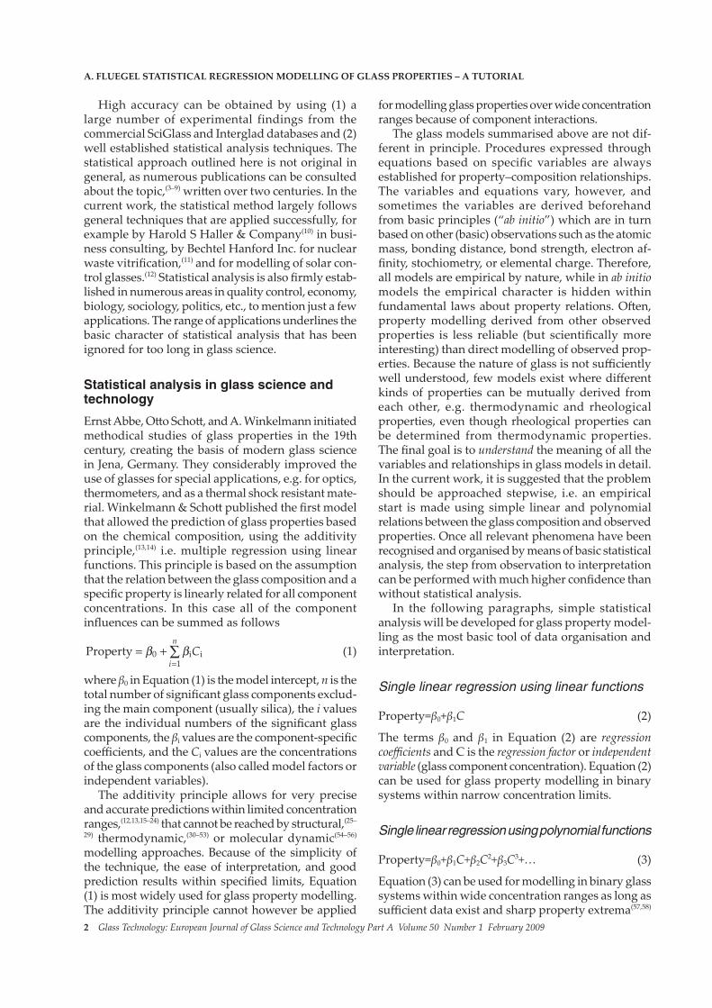
be performed for quantitative evaluation of over/un-der fitting.

The model standard error S derived from the residuals in Table 8 and with five degrees of freedom is 19·4453. Approximately 68% of all residuals fall within the limits of ±S. The standardised residual is the quotient of the residual and the model standard error (the first standardised residual in Table 8 is 1·2376; the second is –0·0291, etc...).

The standard errors of the coefficients Sβ are determined using

Sβ=SCjj1/2=β/tβ (14)

where Cjj are the diagonal elements (marked in bold) of the inverse information matrix (XT.X)–1 in Table 6. The elements Cjj are given in Table 9. The t-value is the ratio of the coefficient and its standard error, as seen in Equation (14). Table 10 summarises all coefficients, including their errors and t-values.

The absolute value of the t-value (also called the t-statistic or t-ratio) is a measure of a coefficient being equal to zero. It is an indicator of the significance of a model factor (variable, component concentration or concentration product (interaction factor)) in slack variable models. In other words, it is a measure of how much information a factor adds to the model. In general, a t-value with an absolute value greater than or equal to two is considered to be significant, with a statistical confidence level of approximately 95%. (This confidence level at t=2 will change slightly with the degree of freedom, but it is at least 90% for DF>4.) Most minor components are insignificant, i.e. their influence is less than the standard error (“noise”). If the t-value of a glass component indicates that its coefficient is insignificant, it should be concluded that its influence on the property being modelled is insignificant within the studied composition range.

It must be noted that t-values may also be calcu-lated and used for models that do not include an intercept following the canonical approach by Scheffé

as seen in Equation (5). The t-values are a measure of a coefficient to equal zero in models with and without intercept. However, it is demonstrated in a paper by Piepel(80) that it is not a meaningful hypothesis to assume that a coefficient equals zero in models without intercept. An alternative component slope mixture model is presented in Ref. 80. For practical application it is advised in this work to always use t-values for evaluating the probability for a coefficient to equal zero for all model forms, with appropriate interpretation of the meaning of the t-values in mod-els without intercept.

Another way of looking at a coefficient significance is possible through consideration of p-values. A p-value reflects the probability of a coefficient being equal to zero, derived from the t-value and the degree of freedom, and is generally based on normal error distribution. The p-value should be lower than 0·05 for a 95% confidence level.

A t-value reflects the significance of a coefficient within the model, but a special application might require a more strict limitation of the composition area than the model is valid for. The narrower the concentration range of a given component, the more and more a coefficient becomes practically insignificant.

It is obvious in Table 10 that the errors of the coef-ficients βB, βC, βD are larger than their absolute values or of comparable size, and that the absolute values of their t-values are smaller than two. It is not pos-sible with reasonable certainty to conclude whether the glass components B, C, and D have a significant influence within the examined composition range. Consequently, the glass components B, C, and D may be excluded from further calculations (Table 11). This exclusion must be performed stepwise because based on correlations it frequently happens that after exclu-


Table 8. Example model residualsPropertyobserved calculated residual69·4 45·3345 24·065515·8 16·3663 −0·566318·6 19·1862 −0·586230·8 41·5975 −10·797525·7 37·8155 −12·115571·1 80·1982 −9·098262·5 70·4203 −7·920353·3 65·2396 −11·939664·1 62·6605 1·439593·4 65·8814 27·5186

Table 9. Example Cjj values from Table 6Intercept 1·05733βB 0·01358βC 0·01125βD 0·02881Offset L1 0·48966

Table 10. Example model coefficients, coefficient standard errors, and t-valuesVariable Coefficient Sβ tβ

Intercept 81·5743 19·9949 4·0798βB 0·3096 2·2659 0·1367βC 1·7997 2·0628 0·8725βD −4·9981 3·3008 −1·5142Offset L1 −31·5514 13·6070 −2·3188

Table 11. Example factor matrix, after exclusion of the components B, C, and DIntercept Offset L11 11 11 11 11 11 01 01 01 01 0

Glass Technology: European Journal of Glass Science and Technology Part A Volume 50 Number 1 February 2009 ��

sion of one insignificant variable another previously insignificant one becomes significant. In the example described here this is not the case.

The exclusion of components B, C, and D in the given example is called stepwise backward elimination, as initially all possible variables were included in the model, and the insignificant ones were excluded stepwise. The opposite approach would be stepwise forward selection, i.e. the most significant variable is included first in the model, followed by the next significant one, until no further significant variables can be found. During stepwise backward elimination and forward selection the factor hierarchy described above in the section “Step 4: Correlation analysis” should be taken into account.

For analysing large glass databases it is recom-mended to proceed stepwise as follows: (1) selection of all significant single glass components through backward elimination; (2) selection of the most sig-nificant and scientific reasonable two-component in-teraction factors (boron anomaly, mixed alkali effect) through forward selection; (3) analysis of systematic offsets in whole data series from selected laboratories and if necessary exclusion of those series that are incomparable with the majority of all other series;(81,82) (4) stepwise deletion of outliers and simultaneous selection/elimination of variables according to their significance and scientific reason until no further outlier can be found.

Models that include insignificant variables are termed over fitted, and often are unrealistically well fitted.

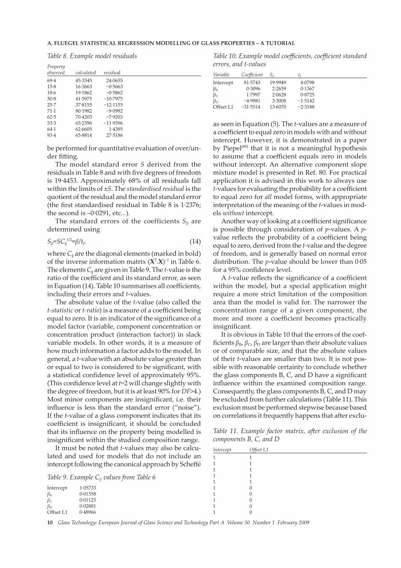
Next, it is necessary to repeat the procedure, beginning with Step 5 (determination of the model coefficients). The size of the inverse information matrix decreases to 2×2 (Table 12).

Table 13 shows the new coefficients, coefficient standard errors, and t-values. The new model stand-ard error S is 18·6893, which is insignificantly lower than the previous value of 19·4453. Table 14 gives the new model residuals.

Step 7: Outlier analysis, data leverage

From the residuals in Table 14, it can be concluded that some of them seem to stand out from others. It is possible that experimental or data entry problems caused a datapoint to show an anomalous response or that the composition is outside the range where the linear approximation of component effects is valid. The latter can be checked easily by comparing

the compositions of the outliers to other glasses in two dimensions (see Figure 3), or through leverage analysis, described below in this section.

Regression analysis assumes that the residuals are normally distributed. Thus, a datapoint may be regarded as an outlier:(10)

(1) if the absolute of the residual is larger than about three times the model standard error (=absolute of standardised residual larger than about three),

(2) if the largest residual is higher than about 1·5 times the next largest residual, or

(3) if the externally studentised* residual is higher than about three.

It is always possible to refer to the p-statistic (see above in the previous section, Step 6) to determine exact critical outlier limits using the desired confi-dence level such as 99·7%. However, in most cases, the approximate limits stated here are sufficient.

Understanding of the outlier conditions (1) and (2) can be derived from the explanations above. To clarify the meaning of the outlier condition (3), more details must be given about data leverage in statistical analysis.

The h-value measures how much “leverage” a par-ticular row of data could have on the resulting overall correlations. It is also known as the Hat diagonal value, or diagonal value hi of the Hat-matrix H. It is a measure of how good the experimental design is for all the variables in the model. In Figure 3 is a two-dimensional example of a point with a high h-value. One glass composition with high h-value stands out from all other compositions. The Hat-matrix H and


Table 12. Example inverse information matrix (XT·X)−1, after exclusion of the component B, C, and D Intercept Offset L1Intercept 0·� –0·2Offset L1 –0·2 0·�

Table 13. Example model coefficients, coefficient standard errors, and t-values, after exclusion of the component B, C, and DVariable Coefficient Sβ tβ

Intercept 68·8800 8·35811 8·2411Offset L1 −36·8200 11·8202 −3·115

Table 14. Example model residuals, after exclusion of the component B, C, and DPropertyobserved calculated residual69·4 32·0600 37·340015·8 32·0600 −16·260018·6 32·0600 −13·460030·8 32·0600 −1·260025·7 32·0600 −6·360071·1 68·8800 2·220062·5 68·8800 −6·380053·3 68·8800 −15·580064·1 68·8800 −4·780093·4 68·8800 24·5200

* The expression "studentised" is not a typographic error; "studentised" is different from "standardised." The term is in honor of the English statistician William Sealey Gosset (1876–1937) who published under the pseudonym "Student."

1� Glass Technology: European Journal of Glass Science and Technology Part A Volume 50 Number 1 February 2009

the h-value hi are defined by

H=X.(XT.X)-1XT

hi=xiT.(XT.X)-1.xi (15)

Table 15 shows the example Hat-matrix determined from the factor matrix in Table 11. The h-values hi de-rived from the factor matrix in Table 11, are marked in bold and underlined. In the example described here, all experiments have the same leverage by chance. Please note that the sum of all h-values is exactly two, the number of variables in the model, including the intercept. The rule-of-thumb is that a glass composi-tion has a high amount of leverage when the h-value is higher than two times the quotient of the number of variables including the intercept, over the number

of experimental datapoints.(83) In the example above, it would mean that experiments have a large leverage if h is higher than 2×2/10, i.e. 0·4.

It is not recommended that a glass composition be deleted solely on the basis of its h-value.

While the leverage of a glass composition on the overall correlations is quantified by its h-value, the leverage of one experiment on the model result (i.e. the coefficients) is measured with the Cook value, defined in Equation (16).(84,85) The Cook value compares the model result (coefficients) with and without each experiment. Generally, an experiment with a Cook value larger than one has a high leverage. One should make sure that an experiment with a high Cook value is ac-curate, e.g. a NIST (National Institute for Standards and Technology) or DGG (German Society of Glass Technology) glass property standard; otherwise, the whole model might suffer from one single high leverage datapoint

Cookii i

i=

-( )D2

2 21h

pS h (16)

where p is the number of model variables including the intercept (=2 in Table 13). Table 16 lists the Cook values of all experiments from the model in Tables 11 to 14. The first experiment has a much higher Cook value (Cook=0·6237) than all others, but which is


Table 15. Example Hat-matrix H, derived from Table 11 1 2 3 4 5 6 7 8 9 101 0·� 0·2 0·2 0·2 0·2 0 0 0 0 02 0·2 0·� 0·2 0·2 0·2 0 0 0 0 03 0·2 0·2 0·� 0·2 0·2 0 0 0 0 04 0·2 0·2 0·2 0·� 0·2 0 0 0 0 05 0·2 0·2 0·2 0·2 0·� 0 0 0 0 06 0 0 0 0 0 0·� 0·2 0·2 0·2 0·27 0 0 0 0 0 0·2 0·� 0·2 0·2 0·28 0 0 0 0 0 0·2 0·2 0·� 0·2 0·29 0 0 0 0 0 0·2 0·2 0·2 0·� 0·210 0 0 0 0 0 0·2 0·2 0·2 0·2 0·�

Figure 3. h-value demonstration

Table 16. Example model statistics, model from Table 13Property Residual h Cook Press Si ESobserved calculated ∆ value value residual residual69·4 32·0600 37·3400 0·2 0·6237 46·6750 13·2324 3·154915·8 32·0600 −16·2600 0·2 0·1183 −20·3250 18·7521 −0·969518·6 32·0600 −13·4600 0·2 0·0810 −16·8250 19·0956 −0·788130·8 32·0600 −1·2600 0·2 0·0007 p1·5750 19·8167 −0·071125·7 32·0600 −6·3600 0·2 0·0181 −7·9500 19·6629 −0·361671·1 68·8800 2·2200 0·2 0·0022 2·7750 19·8036 0·125362·5 68·8800 −6·3800 0·2 0·0182 −7·9750 19·6619 −0·362853·3 68·8800 −15·5800 0·2 0·1086 −19·4750 18·8421 −0·924564·1 68·8800 −4·7800 0·2 0·0102 p5·9750 19·7327 −0·270893·4 68·8800 24·5200 0·2 0·2690 30·6500 17·2919 1·5854


smaller than one, i.e. it is still not significant. If the first experiment were removed from the discussed model example, the coefficients would change the most.

The Press residual is the quotient of the residual over (1−h), as given in Table 16. Press is the residual that would occur for a given experiment if that experi-ment were not included in the regression analysis calculation, but rather if it were predicted by a model including all other experiments. Hence, an experi-ment with high leverage on the model (Cook value) would have a high Press residual as well.

The h-value also makes it possible to determine the model standard error if one experiment were excluded (Si) using

Si={[(DF+1)S2−Δi2/(1−hi)]/DF}1/2 (17)

In Table 16, it becomes clear that if the first experi-ment were excluded from the model, then the model standard error would decrease much more than for all other experiments. In the final step of the outlier analysis, the externally studentised residual (ES re-sidual) may be derived from Si using

ES residual=Δi/[Si(1−hi)1/2] (18)

The ES residual is a more sensitive outlier indicator than the residual Δ alone, because the data leverage is considered. The analysis of the ES residuals makes consideration of the generally employed studentised residuals, which do not take into account Si from Equa-tion (17) and which do not have a true t-distribution, obsolete. Table 16 displays all ES residuals from the model example above.

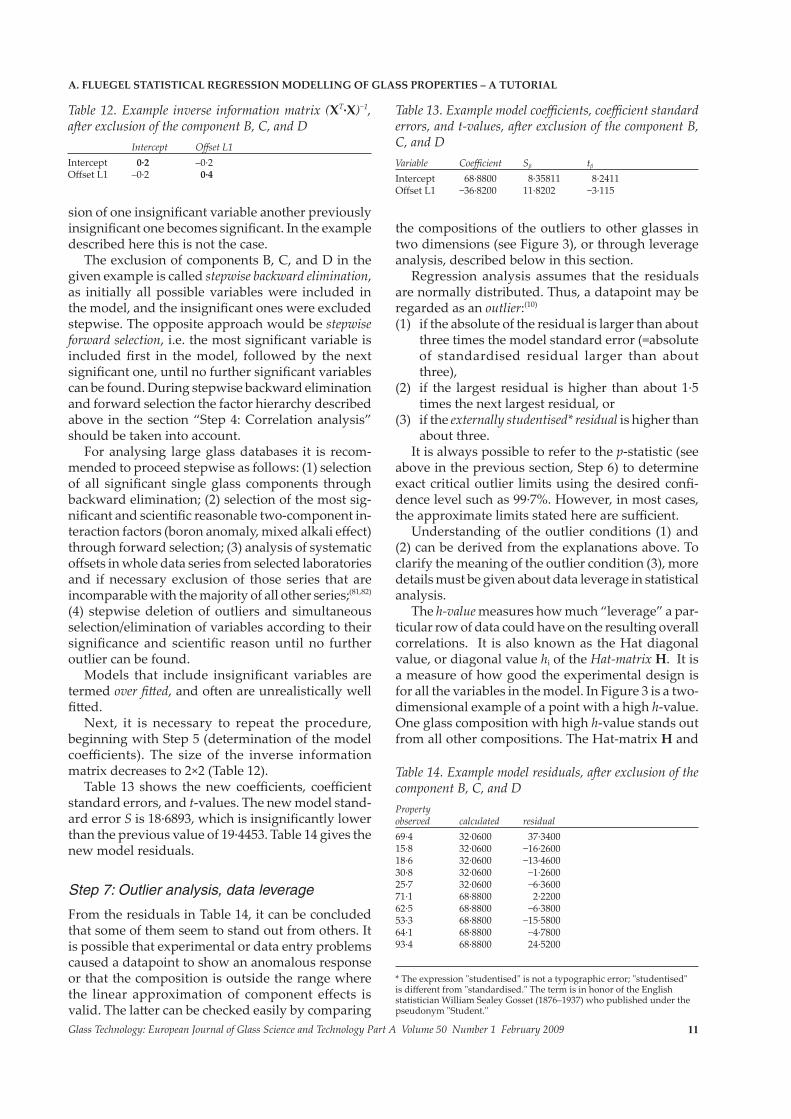
From the statistical indicators in Table 16, it can be concluded that the first experiment is probably an outlier. It should be evaluated in detail by an expert in the subject and excluded from the source database if deemed reasonable; the modelling procedure should then be started all over again, beginning with Step 4 (correlation analysis). Table 17 shows the new correlation matrix, Table 18 shows the final model, and Table 19 shows further statistical indicators. No further outlier can be detected. In the final model the last experiment has a relatively high leverage (Cook=0·9230), which is still lower than one, i.e. it is still considered to have an insignificant leverage on the model. However, during model validation it should be evaluated if the experimental result is reliable.

In the given example it turns out that there exists a systematic difference between the data from Labora-tory 1 and Laboratory 2. The calibration procedure for the new measurement method attempted in Laboratory 1, stated above in connection with Table 1, must be re-evaluated.

Systematic errors in whole measurement series that lead to an offset are known in the glass science literature.(65,86)

Step 8: Goodness-of-fit evaluation, validation, model improvementThe goodness of a model fit (the measure of how well the glass properties can be described with the given glass compositions) is generally expressed in R2 values, defined by

R2=1−{Σ(Δ2)/Σ[(Observation−Average observation)2]} (19)

R2, adjusted=RA2=1−[(1-R2)(n-1)]/DF (20)

R2, predicted= RP

2=1−{(Press2)/Σ[(Observation−Average observation)2]} (21)

R2, also known as coefficient of determination, is a gen-eral goodness-of-fit indicator for models including an intercept (slack variable) that shows the fraction of the total variance in the dependent variable (glass property) that is explained by the model. If R2 is close to one, it either means that the model is good or that it could be the result of over fitting with insignificant and correlated variables.

R2 can be calculated and interpreted for the models described in this work with and without an intercept (Equation (5)).(87) However, the reader should be aware of the fact that in some model forms with a forced intercept R2 is not defined,(88,89) and some software packages calculate R2 incorrectly or do not permit its calculation at all. For glass property modelling described in this study R2 should only be determined using Equation (19).

RA2, originally established for models without an

intercept (Ref. 6, p 532), is adjusted for the degrees of freedom in multiple regression. If RA

2 is significantly lower than R2, it can be concluded that the model is over fitted. Therefore, RA

2 is often a better goodness-of-fit indicator than R2 for multiple regression.

RP2, also called R2

PRESS, is calculated in the same way as R2, but using the Press residuals instead of the residuals. RP

2 shows the expected fraction of the variance in the dependent variable (glass property) that can be explained by the model for predicting new experiments. If RP

2 is significantly lower than R2 and RA

2, it means that some experiments have a high leverage.

The model discussed above has relatively high R2 values, with R2=0·9678, RA

2=0·9485, and RP2=0·8743;

i.e. the model fit appears to be good. RP2 is somewhat

lower than R2 and RA2 because of the last high leverage

datapoint. The last datapoint may be re-evaluated.In glass property modelling using statistical analy-

sis the values of the R2 indicators are often higher than 0·9,(16–21,60,61,64,65) especially for properties that are relatively easy to measure such as the viscosity. For properties that are difficult to obtain, e.g. gas solubilities in glass melts, R2 tends to be lower.(20) In



general, R2 values higher than 0·8 may be considered as good.

A good model fit could be a sign of reproducible experiments; further hidden variables are unlikely to be discovered (correlations not considered). It is not clear yet, however, which one of the strongly correlated glass components B and E is causing the observed property changes. Add on experiments should be performed for decorrelating the glass components B and E. Table 17 also shows that some weaker correlations still remain, which always needs to be considered during interpretation of the model results. Some variables are not completely statistically independent. Therefore, it should be preferred to interpret model predictions rather than individual coefficients.

For model evaluation, the residuals should be plotted against the experimentally observed property values and against the calculated property values. Ideally, the result would be as shown in Figure 4, i.e. the residuals are normally distributed. However, if a residual variance trend occurs as displayed in Figure 2, logarithmic data transformation for error normalisation may be evaluated. If a plot is obtained as in Figure 5, the model may still not include an important variable.

The residuals also should be plotted against each variable. A pattern as seen in Figure 6 indicates that a squared term for the considered variable (glass component 1) should be introduced.

If stepwise residual trends occur, “block effects” may be present. Some data series may be different

than others (different property values), or the errors within various data series may be different.

For statistical model validation, the differences between precision (repeatability), reproducibility, and accuracy must be taken into account. The precision reflects the consistency and repeatability within a data series of one experienced investigator, generally using one measurement technique. The reproduc-ibility is a measure of how well other experienced investigators in other laboratories can reproduce the experiment. The accuracy shows the similarity to the “true” or “mean” value in case the absolute truth is known. It is often assumed that experiments reproduced by several experienced and independent investigators are very close to being accurate, e.g. NIST or DGG glass property standards.

Consequently, for models based on one single investigator, a reproducibility and accuracy can not be established; only the precision may be evaluated. However, in high quality publications that contain experimental data the author is always using external values for calibration and/or comparison. Therefore, even for some models based on one single study repeatability and accuracy can be established. For models based on several investigators, the reproduc-ibility may be determined, which can be assumed to come close to accuracy if many investigators agree. Statistical model validation can be obtained by:(1) Splitting of the source data into one set for model-

ling and a second set for comparing of predicted and experimental data;

(2) Comparing the model predictions to experimen-tal data from another investigator;

(3) Comparative modelling of two data series from different investigators where coefficients and residual trends are compared with and without the second series;

(4) Comparative modelling of several data series from various investigators including careful


Table 17. New linear correlation matrix B C D E Offset L1B 1 C –0·269 1 D –0·159 0·298 1 E –0·990 0·321 0·210 1 Offset L1 0·000 –0·183 0·328 –0·016 1

Figure 4. Normal residual distribution


analysis of correlations, over/underfitting, sys-tematic trends, and data leverage;

(5) Developing two independent models based on data series from different investigators in similar composition regions and comparing the model coefficients considering correlations, and

(6) Developing two independent models, including all possible component interactions based on data series from different investigators in different composition regions (compositions in mol%) and comparison of the model coefficients considering correlations.

If the standard errors are comparable to the errors found during model evaluation and correlations/trends are considered, it can be assumed that the model is accurate, i.e. it is “validated.” Method (1) can be used for an internal validation of the model precision, and methods (2) to (6) allow conclusions to be drawn concerning total accuracy by comparing the results with other investigators.

In addition to standard error comparison, it is

also possible to determine R2, validation= RV2. RV

2 is calculated in the same way as R2 in Equation (19), but instead of the model residuals, the residuals from the validation test are used. For example, a model may be established based on 80% of all data, and then predictions are made for the remaining 20%, and only the residuals of the 20% of the data are considered for the RV

2 calculation.An experimental model validation is superior to the

statistical validation explained above. In addition, it is often possible with experimental model validation to improve the model considerably, resulting in a prediction error reduction up to 20 to 50% according to the experience of the author. Experimental valida-tion and model improvement should be approached as follows:(1) First, the reasonability of dataset-specific categor-

ical offset variables must be examined. It has to be investigated experimentally if and how find-ings from different laboratories are comparable. The most contradictory findings from different


Figure 5. Residual trend

Figure 6. Residual trend versus a variable (glass component 1)


laboratories should be reproduced.(2) The glasses with the greatest influence on the

overall understanding (high Cook values) need to be re-analysed and/or remelted and excluded from the model if crystallisation or phase separa-tion occurs, if undissolved batch material remains in the glass, if the bubble content is very high, if extremely strong striations are visible, or if other similar irregularities can be observed.

(3) The model result (glass component influences on the property) should evaluated from a glass science standpoint. It must be estimated whether the model is reasonable and makes any scientific sense. Surprising or unusual glass component influences need to be traced back to the indi-vidual glasses that are the most significant causes of these influences, and those glasses have to be remelted and measured. For example, if all glass components influence the property for up the 10 property units per mol%, and one minor component appears to influence the property for 5000 property units per mol%, then it is pos-sible that this phenomenon is rather difficult to understand scientifically. The mentioned minor component with the exceptional influence should be analysed experimentally.

(4) Finally, add-on experiments can be performed to reduce mutual correlations of glass components, and to expand the model into new composition areas.

In general, a good multiple regression model has the following properties:(10)

· All factors in the model are significant (absolute value of t-values>2), and all excluded factors are insignificant (absolute value of t-values<2), i.e.

there are no over/under fitting occurs.· Accurate predictions can be made using the model.

The standard error of the model S is not signifi-cantly (no more than about 1·7 times) larger than the standard deviation of repeated experiments from several investigators.

· The standard error of the model S is higher than the standard deviation of repeated experiments from several investigators, i.e. the model is not over-fitted.*

· The coefficients are reasonable, according to the judgment of experts familiar with the modelled property.

· Follow-up experiments within the model applica-tion limits agree with the model predictions.

Step 9: Model application

For all glass property models published in the litera-ture, the compositional area is defined for which the model is valid. Those composition limits are stated as minima and maxima of all glass components consid-ered in the specific model. However, in many cases, it may happen when two or more concentrations are set to extrema that those extreme combinations were not investigated in fact, even though the extreme single component influences were. Consequently, models may result in inaccurate predictions for


Figure 7. Binary 95% component combination limits; 95% of all data are within the limits of the ellipse. Please note that the limits are not characterised by a rectangle instead of the ellipse shown. The corners of a rectangle would be outside the source data, which is not considered in almost all glass property models

* It is often impossible to estimate the standard deviation of repeated experiments from several investigators because of the lack of data for multicomponent glasses. Therefore, it is advised to collect all published values available from binary glass systems.(78) A polynomial fit of the second or third degree often describes those data well. The standard error obtained from binary systems may be assumed to be similar to the error concerning multicomponent glasses.


Table 18. Final example model coefficients, coefficient standard errors, t-values, and model standard errorVariable Coefficient Sβ tβ

Intercept 36·4174 7·3308 4·9678βB 3·1107 0·8195 3·7960βC 2·3791 0·6113 3·8915Offset L1 −43·0622 4·1720 −10·3218βD 0 insignificantS=6·1053

certain component combinations if the combination (i.e. interaction) limits are not well defined.

The component combination limits for glass property models state the maxima and minima of all compo-nent combinations that are covered by the model. The component combination limits need to be specified in addition to the concentration limits of all glass components.

Given the uncorrelated components 1 and 2 with normally distributed concentration values, the binary component combination limits may be expressed as seen in Figure 7 and defined using

U2=s2/s1[(tα.DFs1)2−(c1−a1)2]1/2+a2 (22)

L2=−s2/s1[tα.DFs1)2−(c1−a1)2]1/2+a2 (23)

where U2, L2 are the upper and lower concentration limits of component 2, s1, s2 are the standard de-viations of all concentration values of components 1 and 2, a1, a2 are the average concentrations of the components 1 and 2 and c1 is the concentration of component 1. Ternary component combination limits can be similarly derived from a spherical function like f(x,y)=(radius2−x2−y2)1/2.

If the components 1 and 2 in Equations (22) and (23) are linearly correlated the constant term a2 in the Equations (22) and (23) would need to be replaced by a linear function c2=slopec1+intercept.

Equations (22) and (23) can be applied in many cases for glass property modelling if the compo-nent 1 is silica (SiO2), i.e. most binary component combination limits [(SiO2)–(other component)]

can be quantified through Equations (22) and (23). However, it is not possible to use Equations (22) and (23) for component combination limits of most of the remaining glass components besides SiO2 because of a non-normal distribution of the data. For practical application, it is beneficial to define the component combination limits as follows:(1) Maxima and minima of component concentra-

tion products (minima mostly zero)=interaction variables in Equation (7),

(2) Maxima and minima of component concentra-tion sums (e.g. for excluding binary glasses like SiO2–CaO or ternary glasses like SiO2–B2O3–Al2O3 from model predictions that are not part of the source data),

(3) Maxima of the terms (SiO2+Na2O).SiO2, (SiO2+K2O).SiO2, (SiO2+PbO).SiO2, and similar terms for excluding predictions in the binary systems SiO2–Na2O, SiO2–K2O, SiO2–PbO, etc. at high concentrations of SiO2.

In addition, model predictions should be con-sidered unreliable if the 95% prediction confidence interval SCI given below in Equation (26) is higher than three times the model standard error S.

Model predictions can be made using Equations

(1) or (7).The standard prediction error of the mean for a glass

composition of interest (PE, prediction error) can be determined using

PE=S[x0T(XTX)−1x0]1/2 (24)

with x0 being the factor 1-column matrix derived from the glass composition of interest, and x0

T be-ing its 1-row transpose. PE is generally lower than S. For example, if the PE is determined for a glass from Laboratory 2 containing 3% B and 5% C, the matrix x0

T would be [1|3|5|0], and the prediction is 57·6448±2·3579 (PE=2·3579). This means that there is a confidence of about 68% (tα,DF~1) that the average property of multiple glass samples with the desired composition would be as predicted with an error of ±2·3579. PE is also a measure for the model sensibility limit, i.e. how large model prediction differences must be to represent a real difference, and below which any small differences may be considered as zero. With a model prediction difference of PE and tα,DF>3, there is a confidence of about 62% that the different predictions are equal; with a difference of about 0·12×PE this confidence increases to 95%, and with a difference of about 3·9×PE the confidence decreases to 5%. It should be the goal to keep this confidence low. That means for slightly different model predic-tions it is desirable to make sure that the predictions are not equal.

The standard confidence interval of the mean model prediction is obtained by multiplying the standard prediction error PE by the t distribution value tα,DF. For a 95% confidence and DF>15, tα,DF can be approxi-mated as 2. DF=5 for the model described above.

Naturally, the standard error for predicting a single future experiment (PEF, prediction error for a single future experiment) is higher than the standard error for the predicting the mean response (PE). The PEF may be estimated using

PEF=(S2+PE2)1/2 (25)

Comparing PE and PEF demonstrates the fact that single experiments from one laboratory are less valuable than the modelled mean of a number of reproduced experiments for evaluating property values.

The standard prediction confidence interval of the mean for multiple glass compositions or the simulta-



neous confidence interval of the mean

SCI=PE(pFα.p.DF)1/2 (26)

reflects the certainty that all of several predicted values are within the specified range with the desired confidence (S-method(90)). SCI should be preferred over PE in glass technology because it shows the con-fidence related to mass production. The 95% SCI for a glass containing 3% B and 5% C following the model in Tables 18 and 19 is 57·6448±10·7454 (SCI=10·7454 with F95%,4,5=5·1922). If the glass containing 3% B and 5% C were mass produced, then 95 out of 100 glasses are predicted to have the desired property with an error of ±10·7454 because of model uncertainty.

The prediction errors PE, PEF, and SCI described above are valid only if the chemical glass composition is known exactly. However, the chemical composition within a glass melting tank may vary, and the accu-racy of a chemical analysis of a sample from the glass tank may vary as well. For a good estimation of the predicted property error, the chemical composition variation within a glass melting tank must be quanti-fied through chemical analysis. If the glass composi-tion in the tank is systematically different in specific locations, those different compositions should be used for property prediction within those locations. In case the glass composition varies randomly, several measurements should be taken, and the standard de-viation of each glass component, which is the result of random variations of the chemical composition in the tank and the analytical measurement error, should be calculated. The glass composition uncertainty can now be converted to a property prediction confidence interval due to chemical uncertainty (PCIC) using

PCIC=tα.DF(coT.Sc.co)1/2 (27)

with co being the 1-column coefficient matrix from Equation (12). The degrees of freedom DF in Equation (27) may be assumed to equal the number of samples

used to determine the Sc (see below) minus one.The chemical composition variance matrix Sc (S

for σ2, C for chemical) in Equation (27) is defined in Table 20. It consists of a diagonal matrix that contains the square of the standard deviation σ2 (=variance) for each glass component included in the model as diagonal elements, and zero in all other matrix positions. In case the model included squared or interaction variables according to Equation (7), they need to be considered in the chemical composition variance matrix as well. If the main glass component silica (SiO2) were excluded following the slack-vari-able technique in Equations (1) and (7) the matrix co should be recalculated according to the canonical model form in Equation (5) following equations listed by Piepel (Ref. 91, p 190) and Cornell (Ref. 6, p 15–18 and 333–343).

The total prediction confidence interval CItotal caused by model uncertainty and the uncertainty of the chemical glass composition to be predicted is the sum of SCI and PCIC

CItotal=SCI+PCIC (28)

The technique described in this work can be suc-cessfully applied for glass property modelling as demonstrated in previous papers.(20,64,77)

Analysis summary

The advantages of the presented statistical analysis method may be summarised as follows:Superior accuracy: The large number of source data

points allows a higher accuracy than the error arising from a few experiments.

Time and financial savings: Calculations can be completed within minutes. In contrast, one single experimental investigation may take several hours or days, including large personnel and equipment expenses, and the measurement ac-


Table 19. Final example model statistics, model from Table 18Property Residual h Cook Press Si ESobserved calculated ∆ value value residual residual15·8 9·8244 5·9756 0·4678 0·3955 11·2277 5·5957 1·463818·6 25·5620 −6·9620 0·3123 0·2147 −10·1236 5·5348 −1·516830·8 34·1624 −3·3624 0·4166 0·0928 −5·7633 6·3917 −0·688725·7 21·3511 4·3489 0·5159 0·2792 8·9836 6·0759 1·028771·1 66·4295 4·6705 0·5416 0·3770 10·1882 5·9341 1·162562·5 65·5136 −3·0136 0·2689 0·0306 −4·1217 6·4997 −0·542253·3 57·4604 −4·1604 0·4310 0·1546 −7·3120 6·2166 −0·887264·1 66·0608 −1·9608 0·3610 0·0228 −3·0684 6·5975 −0·371893·4 88·9357 4·4643 0·6850 0·9�30 14·1736 5·6635 1·4045

Table 20. Chemical composition variance matrix (SC) Component 1 Component 2 Component 3 Component 4 Component 5Component 1 σ1

� 0 0 0 0Component 2 0 σ�

� 0 0 0Component 3 0 0 σ3

� 0 0Component 4 0 0 0 σ�

� 0Component 5 0 0 0 0 σ5

�



curacy still needs to be confirmed statistically afterwards by comparing results with those of other investigators.

Compatibility: Multiple regression makes data com-parable over wide composition ranges, different measurement techniques, and from various investigators. Previous glass property models can be integrated (e.g. Lakatos et al; Hrma et al).(20) Without multiple regression, only data in binary glass systems are directly comparable.

Broad application range: The accuracy of new measurements mostly cannot be derived directly from similar results in the scientific literature or from NIST or DGG glass property standards. The multiple regression modelling approach may include several glass types with different chemi-cal compositions; it makes them comparable. Consequently, the model allows predictions in composition areas that are not covered by com-mon industrial models that are valid for only one specific glass type. The results of experiments inside and outside conventional ranges can be predicted and compared economically.

Future work

It is recommended that the demonstrated method be applied to all experimental values in the databases SciGlass(1) and Interglad(2) for “cleaning up” and organising the large volume of collected data, as in the work started by the author.(64,77) For example, up to now, such a well investigated glass property as the Littleton softening point in a simple binary system like SiO2–Na2O is not known exactly, as demonstrated through Table 21 and Figure 8. For other less inves-tigated properties and multicomponent glasses, the uncertainties are more significant. It is necessary to quantify property values and the corresponding errors in detail.

The quality of the experimental data published by various authors should be evaluated based on statistical procedures described in this work and knowledge of the subject matter, including systematic offsets of whole series and the residual scattering compared with other investigators. A “quality rating” for publications, authors, or institutions would help to significantly improve the accuracy of property predictions.

In the future, systematic experiments should be performed to fill the numerous remaining “blank spots” of glass properties. For instance, little or noth-ing is known about the influences of binary glass component interactions on properties besides very limited information in confined systems concerning mixed alkali effects, boron anomalies, or alumina interactions.

Some steps of the statistical analysis procedure can be automated; hence, it is possible to introduce them into the databases SciGlass(1) and Interglad(2) directly,

Table 21. Littleton softening point in the binary system SiO2–Na2O for Na2O=30–35 mol%Author Year c(Na2O) in mol% L.P. in °CK. S. Evstropiev 1940 34·00 578·6G. S. Meiling 1967 33·46 595·2K. S. Evstropiev 1968 33·30 558·7Shvaiko-Shvaiko 1968 30·00 606·8Shvaiko-Shvaiko 1968 35·00 588·3O. G. Ivanov 1969 30·00 600·2O. V. Mazurin 1970 30·00 600·1K. Matusita 1973 33·30 574·1U. E. Schnaus 1976 33·00 600·8W. H. Dumbaugh 1978 33·31 596·0N. A. Ghoneim 1984 33·33 636·0Y. Shiraishi 1987 33·00 597·0R. Ota 1991 33·30 626·9R. Ota 1995 33·33 613·9M. Liska 1996 33·41 605·6D. Ehrt 1997 33·00 592·5D. B. Dingwell 1998 30·61 585·2D. Ehrt 2001 33·00 587·1Reference: SciGlass Database and Information System 4·0

Figure 8. Littleton softening point in the binary system SiO2– Na2O for Na2O=30–35 mol%

550

560

570

580

590

600

610

620

630

640

29 30 31 32 33 34 35 36

c(Na2O) in mol%

Littl

eton

Poi

nt in

o C a

t log

10(v

isco

sity

/ Pa

·s) =

6.6

Littleton Point in the System SiO2-Na2O

�0 Glass Technology: European Journal of Glass Science and Technology Part A Volume 50 Number 1 February 2009


especially for well investigated properties and within often examined glass composition ranges. It is not recommended to automate all steps described in this work; glass science and statistical expertise must be considered.

The analysis procedure presented in this study is a powerful and economic tool for data organisation and modelling, based on empirical and impartial phenomenology. However, the technique does not allow a detailed scientific understanding of all states and processes within glass, e.g. on the atomic scale. To obtain a better insight into the nature of glass, the simple linear and polynomial equations applied in this work may be replaced by equations with physi-cal meaning such as those described in the nonlinear regression section above.

Conclusions

A statistical analysis method has been presented that enables the modelling of glass properties with high accuracy. It is possible for any user to perform all steps of the analysis in commonly available spread-sheet software.

Statistical analysis allows measurement accuracy to be established through the combined modelling of a high number of original data from different sources. The modelled accuracy is often superior to a few test measurements within one laboratory because of the elimination of the influence of systematically different experimental conditions and/or systematic errors.

The detailed knowledge of glass property–compo-sition relations makes targeted investigations possible with minimal time and financial investment.

The presented statistical analysis technique does not allow a detailed physical understanding of all states and processes within glass, e.g. on the atomic scale. Further work is necessary in this area.

For obtaining highly accurate glass property predictions it is recommended to systematically analyse all available glass databases, and to introduce a “quality rating” for publications.

Acknowledgments

The author would like to thank David Earl (Alfred University) for teaching the basics of statistics and providing very helpful guidance and advice. In addi-tion, special thanks are directed to Alexander Priven (Russia) for reviewing this paper.

References 1. SciGlass 6.5 Database and Information System, 2005. http://www.

sciglass.info/ 2. International Glass Database System INTERGLAD Ver.6; New Glass

Forum, Tokyo, Japan; http://www.ngf.or.jp

3. Montgomery, D. G. Design and Analysis of Experiments, John Wiley & Sons, 2001.

4. Dowdy, S. & Wearden, S. Statistics for Research, John Wiley & Sons, 1983.

5. Myers, R. H. & Montgomery, D. C. Response surface methodology, 2nd edition, John Wiley & Sons, 2002.

6. Cornell, J. A. Experiments with Mixtures - Designs, Models and the Analysis of Mixture Data, Wiley Series in Probability and Statistics, Wiley-Interscience, third edition, January 2002.

7. Draper, N. R. & Smith H. Applied regression analysis, John Wiley & Sons, 1998.

8. Dempster, A. P. Elements of Continuous Multivariate Analysis, Addison-Wesley, New York, New York, 1969.

9. Neter, J., Kutner, M. H., Wasserman, W. & Nachtsheim, Ch. J. Applied Linear Regression Models, third edition, McGraw-Hill/Irwin, 1996.

10. Harold S Haller & Company; 5 Ashley Court; Cleveland, Ohio 44116; USA. http://www.haroldhaller.com/; Bowles, R. L. & Haller: H. S. Advanced Process Improvement Methods; Harold S Haller & Company, Cleveland, Ohio, 1993. User guide of the MCA software, Haller Information Technology System.

11. Piepel, G. F. & Redgate, T. Mixture Experiment Techniques for Reduc-ing the Number of Components Applied for Modeling Waste Glass Sodium Release, J. Am. Ceram. Soc., 1997, �0 (12), 3038–3044. Piepel, G. F., Szychowski, J. M. & Loeppky, J. L. Augmenting Scheffé Linear Mixture Models with Squared and/or Crossproduct Terms, J. Qual. Technol., July 2002, 3� (3), 297–314.

12. Blume, R. & Drummond III, C. Modeling and optimization of solar-control glasses, J. Am. Ceram. Soc., May 2002, �5 (5), 1070–1076.

13. Winkelmann, A. Über die specifischen Wärmen verschieden zusam-mengesetzter Gläser (Heat capacity of various glasses), Annal. Phys. Chemie, 1893, �9, 401–420; Winkelmann, A. & Schott, O. Über die Elastizität und über die Druckfestigkeit verschiedener neuer Gläser in ihrer Abhängigkeit von der chemischen Zusammensetzung (De-pendence of the elasticity and strength of various new glasses from the chemical composition), ibid, 1894, 51, 697–730; Winkelmann, A. & Schott, O. Über thermische Widerstandscoefficienten verschiedener Gläser in ihrer Abhängigkeit von der chemischen Zusammensetzung (Dependence of the thermal resistance of various glasses from the chemical composition), ibid, 1894, 51, 730–746; Winkelmann, A. Über die Elasticitätscoefficienten verschieden zusammengesetzter Gläser in ihrer Abhängigkeit von der Temperatur (Temperature dependence of the elasticity coefficient of various glasses), ibid, 1897, �1, 105–141 (in German).

14. Volf, M. B. Mathematical Approach to Glass, Glass Science and Technol-ogy, vol. 9, Elsevier, 1988.

15. Gehlhoff, G. & Thomas, M. Z. techn. Phys., 1925, �, 544; Z. techn. Phys., 1926, 7, 105 and p 260; Lehrbuch der technischen Physik (Applied Physics), J. A. Barth-Verlag, Leipzig, 1924, p 376 (in German).

16. Lakatos, T., Johansson, L.-G. & Simmingsköld, B. Viscosity tempera-ture relations in the glass system SiO2–Al2O3–Na2O–K2O–CaO–MgO in the composition range of technical glasses, Glass Technol., June 1972, 13 (3), 88–95.

17. Öksoy, D., Pye, D. L. & Boulos, E. N. Statistical analysis of viscosity-composition data in glassmaking, Glastech. Ber. Glass Sci. Technol., 1994, �7 (7), 189–195.

18. Hrma, P. R., Piepel G. F. et al Property/Composition Relationships for Hanford High-Level Waste Glasses Melting at 1150oC; PNL Report 10359 to the US Department of Energy, vol. 1 and 2, Contract DE-AC06-76RLO 1830, December 1994. http://www.osti.gov/dublincore/gpo/servlets/purl/10121755-P8oQTl/webviewable/; http://www.osti.gov/dublincore/gpo/servlets/purl/10121752-cDjMo0/webviewable/; Vienna, J. D., Hrma, P. R. et al Effect of Composition and Temperature on the Properties of High Level Waste (HLW) Glass Melting above 1200oC (Draft); PNNL Report 10987 to the US Department of Energy, Contract DE-AC06-76RLO 1830, February 1996. http://www.osti.gov/dublincore/gpo/servlets/purl/212394-mv0A6T/webviewable/; Hrma, P. & Robertus R. J. Waste glass design based on property composition functions, Ceram. Eng. Sci. Proc., 1993, 1� (11/12), 187–203. Hrma, P., Piepel, G. F., Redgate, P. E., Smith, D. E., Schweiger, M. J., Vienna, J. D. & Kim, D. S. Prediction of processing properties for nuclear waste glasses; Ceram. Trans., 1995, �1, 505–513.

19. Fluegel, A., Varshneya, A. K., Seward, T. P. & Earl, D. A. Viscosity of commercial glasses in the softening range in Proc. Seventh Int. Conf. Advances in Fusion and Processing of Glass III; Ceram. Trans., Volume 141; Eds. J. R. Varner, T. P. Seward & H. Schaeffer, Rochester, New York, USA, 27-31 July 2003, p 379–386; The American Ceramic

Glass Technology: European Journal of Glass Science and Technology Part A Volume 50 Number 1 February 2009 2�


Society, Westerville, Ohio, 2004. 20. Fluegel, A., Earl, D. A., Varshneya, A. K. & Öksoy, D. Statistical analysis

of viscosity, electrical resistivity, and further glass melt properties, Chapter 9 in: High temperature glass melt property database for process modelling, Eds. T. P. Seward III & T. Vascott, The American Ceramic Society, Westerville, Ohio, 2005. http://www.ceramics.org/glassmelt/ http://www.osti.gov/bridge/purl.cover.jsp?purl=/809193-hMVo0M/na-tive/

21. Kucuk, A., Clare, A. G. & Jones, L. An estimation of the surface tension of silicate glass melts at 1400°C using statistical analysis, Glass Technol., Oct 1999, �0 (5), 149–153.

22. Crum, J. V., Schweiger, M. J., Hrma, P. & Vienna, J. D. Liquidus temperature model for Hanford high-level waste glasses with high concentration of zirconia, Proc. 1996 MRS Fall Meeting, 2–6 Dec. 1996, Boston, MA, Materials Research Society, Vol. 465, Scientific Basis for Nuclear Waste Management XX, 1997, p 79–85.

23. Hanni, J. B., Pressly, E., Crum, J. V., Minister, K. B. C., Tran, D., Hrma, P. & Vienna, J. D. Liquidus Temperature Measurements for Modeling Oxide Glass Systems Relevant to Nuclear Waste Vitrification, submitted to Journal of Materials Research.

24. Choudhary, M. K. & Potter, R. M. Heat Transfer in Glass-Forming Melts, Chapter 9 in: Properties of Glass-Forming Melts, Eds L. D. Pye, A. Montenaro & I. Joseph, CRC Press, Boca Raton, Florida, 2005.

25. Appen, A. A. Khimiya Stekla (Glass Chemistry), Leningrad, 1959. (In Russian).

26. Gan, Fuxi New system of calculation of some physical properties of silicate glasses, Sci. Sinica, 1963, 1�, 1365–1391. (In Russian). Gan, Fuxi New system of calculation of properties of inorganic oxide glasses, Sci. Sinica, 1974, 17, 533–551. (In Russian).

27. Demkina, L. I. Physicochemical Principles of the Manufacture of Optical Glass, Izd. Chimia, Leningrad, 1976. (In Russian).

28. Priven, A. I. General method for calculating the properties of oxide glasses and glass-forming melts from their composition and temperature, Glass Technol., Dec 2004, �5 (6), 244–254. http://www.ingentaconnect.com/content/sgt/gt/2004/00000045/00000006/art00001; http://www.sciglass.info/Publications/Priven.pdf and: Priven, A. I. Doctoral Thesis, St. Petersburg, 2002. (In Russian).

29. Priven, A. I. & Mazurin O. V. Comparison of methods used for the calculation of density, refractive index and thermal expansion of oxide glasses, Glass Technol., August 2003, �� (4), 156–166. http://www.ingenta.com/isis/searching/Expand/ingenta?pub=infobike://sgt/gt/2003/00000044/00000004/art00003; http://www.sciglass.info/Pub-lications/PrivenMazurin.pdf

30. Makishima, A. & Mackenzie, J. D. Direct calculation of Young’s modu-lus of glass, J. Non-Cryst. Solids, 1973, 1�, 35–45; and Calculation of bulk modulus, shear modulus, and Poisson’s ratio of glass, ibid, 1975, 17, 147–157; Calculation of thermal expansion coefficient of glasses, ibid, 1976, ��, 305–313.

31. Bottinga, Y., Weill, D. F. & Richet, P. Thermodynamic modeling of silicate melts in Thermodynamics of minerals and melts, Eds R. C. Newton, A. Na-vrotsky & B. J. Wood, Springer-Verlag, Heidelberg, 1981, p. 207–245.

32. Nemilov, S. V. Thermodynamic and kinetic aspects of the vitreous state, CRC Press, Boca Raton, 1995.

33. Pelton, A. D. & Blander, M. Thermodynamic analysis of ordered liquid solutions by a modified quasichemical approach - application to silicate slags, Metallurg. Trans. B (Process Metallurgy), Dec 1986, 17B (4), 805–815.

34. Pelton, A. D. & Wu, P. Thermodynamic modeling in glass-forming melts, J. Non-Cryst. Solids, 1999, �53 (1–3), 178–191. http://dx.doi.org/10.1016/S0022-3093(99)00352-X

35. Chartrand, P. & Pelton, A. D. Modeling the charge compensation effect in silica-rich Na2O-K2O-Al2O3-SiO2 melts; Calphad, June 1999, �3 (2), 219–230. http://dx.doi.org/10.1016/S0364-5916(99)00026-7

36. Kress: V. C. On the mathematics of associated solutions, Am. J. Sci., Oct 2003, 303, 708–722. http://earth.geology.yale.edu/~ajs/2003/Oct/08.03.02Kress.pdf

37. Conradt, R. Thermodynamic Approach to viscosity in the glass transi-tion, Glastech. Ber. Glass Sci. Technol., 1994, �7 (11), 304–311.

38. Conradt, R. Modeling of the thermochemical properties of multicom-ponent oxide melts, Z. Metall./Mater. Res. Adv. Tech., October 2001, 9� (10), 1158–1162.

39. Björkvall, J., Sichen, Du, Stolyarova, V. & Seetharaman S. A model description of the thermochemical properties of multicomponent slags and its application to slag viscosities, Glass Phys. Chem., Mar.–Apr. 2001, �7 (2), 132–147. http://dx.doi.org/10.1023/A:1011332410674

40. Vedishcheva, N. M., Shakhmatkin, B. A. & Shultz, M. M. A simulation

of the thermodynamic properties of oxide melts and glasses, Ceram. Trans., Vol. 29, Eds A. K. Varshneya, D. F. Bickford & P. P. Bihuniak, The American Ceramic Society, 1993, p 283–288.

41. Vedishcheva, N. M. & Shakhmatkin, B. A. Thermodynamic studies of oxide glass-forming liquids by the electromotive force method, J. Non-Cryst. Solids, July 1994, 171 (1), 1–30.

42. Shakhmatkin, B. A., Vedishcheva, N. M., Shultz, M. M. & Wright, A. C. Thermodynamic properties of oxide glasses and glass-forming liquids and their chemical structure, J. Non-Cryst. Solids, 1994, 177 (1), 249–256.

43. Vedishcheva, N. M., Shakhmatkin, B. A., Shultz, M. M. & Wright, A. C. Thermodynamic modelling of glass properties: A practical proposi-tion? J. Non-Cryst. Solids, March 1996, 19�, 239–243.

44. Shakhmatkin, B. A., Vedishcheva, N. M. & Wright, A. C. Can thermo-dynamics relate the properties of melts and glasses to their structure? J. Non-Cryst. Solids, November 2001, �93–�95, 220–226. http://dx.doi.org/10.1016/S0022-3093(01)00674-3

45. Shakhmatkin, B. A. Vedishcheva, N. M. & Wright, A. C. Thermody-namic modeling of the structure of glasses and melts: single-compo-nent, binary and ternary systems, J. Non-Cryst. Solids, November 2001, �93–�95, 312–317. http://dx.doi.org/10.1016/S0022-3093(01)00683-4

46. Schneider, J., Mastelaro, V. R., Zanotto, E. D., Shakhmatkin, B. A., Vedishcheva, N. M., Wright, A. C. & Panepucci, H. Qn distribution in stoichiometric silicate glasses: Thermodynamic calculations and 29Si high resolution NMR measurements, J. Non-Cryst. Solids, Sept 2003, 3�5 (1–3), 164–178. http://dx.doi.org/10.1016/S0022-3093(03)00332-6

47. Besmann, T. M., Spear, K. E. & Beahm, E. C. Thermochemical models for nuclear waste glass subsystems - MgO-CaO and MgO-Al2O3, Materials Research Society Symp. Proc., 1999, 55�, 383–389.

48. Spear, K. E., Besmann, T. M. & Beahm, E. C. Thermochemical modeling of glass: Application to high-level nuclear waste glass, MRS Bull., April 1999, �� (4), 37–44.

49. Besmann, T. M. & Spear, K. E. Thermochemical modeling of oxide glasses, J. Am. Ceram. Soc., Dec 2002, �5 (12), 2887–2894.

50. Besmann, T. M., Spear, K. E. & Vienna, J. D. Extension of the modified associate species thermochemical model for high-level nuclear waste: Inclusion of chromia, Materials Research Society Symp. Proc., 2003, 757, 195–200.

51. Allendorf, M. D. & Spear, K. E. Thermodynamic analysis of silica refractory corrosion in glass-melting furnaces, J. Electrochem. Soc., Feb 2001, 1�� (2), B59–B67. http://dx.doi.org/10.1149/1.1337603

52. Nilson, R. H., Griffiths, S. K., Yang, N., Walsh, P. M., Allendorf, M. D., Bugeat, B., Marin, O., Spear, K. E. & Pecoraro, G. Analytical models for high-temperature corrosion of silica refractories in glass-melting furnaces, Glass Sci. Technol., May/June 2003, 7� (3), 136–151.

53. Strachan, D. M. & Croak, T. L. Compositional effects on the long-term dissolution of borosilicate glass, J. Non-Cryst. Solids, 2000, �7�, 22–33.

54. Tischendorf, B. C., Alam, T. M., Cygan R. T., et al The structure and properties of binary zinc phosphate glasses studied by molecular dynamics simulations, J. Non-Cryst. Solids, Feb 2003, 31� (2–3), 261–272. http://dx.doi.org/10.1016/S0022-3093(02)01795-7

55. Kresse, G. Ab initio molecular dynamics: recent progresses and limi-tations, J. Non-Cryst. Solids, Oct 2002, 31�–31�, 52–59. http://dx.doi.org/10.1016/S0022-3093(02)01649-6

56. Cormack, A. N. & Du, Jincheng Molecular dynamics simulations of soda-lime-silicate glasses, J. Non-Cryst. Solids, Nov 2001, �93–�95, 283–289. http://dx.doi.org/10.1016/S0022-3093(01)00831-6

57. Leko, V. K., Gusakova, N. K., Meshcheryakova, E. V. & Prokhorova, T. I. The effect of impurity alkali oxides, hydroxyl groups, Al2O3, and Ga2O3 on the viscosity of vitreous silica, Glass Phys. Chem., May–June 1977, 3 (3), 204–219.

58. Dreyfus, C. & Dreyfus, G. A machine learning approach to the esti-mation of the liquidus temperature of glass-forming oxide blends, J. Non-Cryst. Solids, 2003, 31�, 63–78. http://dx.doi.org/10.1016/S0022-3093(02)01859-8

59. Scheffé, H. Experiments with Mixtures, J. R. Statistical Soc. B, 1958, �0, 344–360.

60. Lyon, K. C. Prediction of the Viscosities of Soda-Lime Silica Glasses, J. Res. Nat. Bur. Standards A, Phys. Chem., July–Aug 1974, 7�A (4), 497–504.

61. Kucuk, A. Structure and the physicochemical properties of glasses and glass melts, Doctoral Thesis, Alfred University, New York, 1999.

62. Rao, Q., Piepel, G. F., Hrma, P. & Crum, J. V. Liquidus temperatures of HLW glasses with zirconium-containing primary crystalline phases, J. Non-Cryst. Solids, Oct 1997, ��0 (1), 17–29. http://dx.doi.org/10.1016/

�� Glass Technology: European Journal of Glass Science and Technology Part A Volume 50 Number 1 February 2009


S0022-3093(97)00227-5 63. Backman, R., Karlsson, K. H., Cable, M. & Pennington, N. P. Model for

liquidus temperature of multicomponent silicate glasses, Phys. Chem. Glasses, 1997, 3� (3), 103–109.

64. Fluegel, A., Earl, D. A., Varshneya, A. K. & Seward, T. P. Statistical analysis of glass melt properties for high accuracy predictions: Density and thermal expansion of silicate glass melts, Proceedings CD, DGG Meeting, Würzburg, Germany, 23–25 May 2005. http://glassproperties.com/density/

65. Fluegel, A., Varshneya, A. K., Earl, D. A., Seward, T. P. & Oksoy, D. Improved composition-property relations in silicate glasses, part I: viscosity, Ceram. Trans., 170, Melt Chemistry, Relaxation, and Solidifica-tion Kinetics of Glasses - Proceedings of the 106th Annual Meeting of the American Ceramic Society, 2005, p 129–143. http://glassproperties.com/viscosity/

66. Russell, J. K. & Giordano, D. A model for silicate melt viscosity in the system CaMgSi2O6-CaAl2Si2O8-NaAlSi3O8, Geochim. Cosmochim. Acta, 2005, �9 (22), 5333–5349.

67. Karlsson, K. H., Backman, R., Cable, M., Peelen, J. & Hermans, J. Estimation of liquidus temperatures in silicate glasses, Glass Sci. Technol. (Glastech. Ber.), July 2001, 7� (7), p 187–191.

68. Vienna, J. D., Hrma, P., Crum, J. V. & Mika, M. Liquidus temperature-composition model for multi-component glasses in the Fe, Cr, Ni, and Mn spinel primary phase field, J. Non-Cryst. Solids, November 2001, �9� (1–3), 1–24.

69. Hrma, P., Smith, D. E., Matyáš, J., Yeager, J. D., Jones, J. V. & Boulos, E. N. Effect of Float Glass Composition on Liquidus Temperature and Devitrification Behavior, accepted for publication by Journal of Glass Science and Technology.

70. Redgate, P. E., Piepel, G. F. & Hrma, P. R. Second-Order Model Selec-tion in Mixture Experiments, p 104–110 in 1992 Proceedings of the Section on Physical and Engineering Sciences, American Statistical Association, Alexandria, VA, 1992.

71. Hastie, J. W. & Bonnell, D. W. A predictive phase-equilibrium model for multicomponent oxide mixtures: Part II. Oxides of Na-K-Ca-Mg-Al-Si, High Temp. Sci., June 1984, 19 (3), 275–306.

72. Bishop, C. Neural Networks for Pattern Recognition, Oxford University Press, 1995.

73. Rousseeuw, P. J. & Leroy, A. M. Robust Regression & Outlier Detection, Wiley, 1987.

74. Huber, P. J. Robust Statistics, Wiley, 1981. 75. Hunold, K. & Brückner, R. Physikalische Eigneschaften und struk-

tureller Feinbau von Natrium-Alumosilicatgläsern und -schmelzen (Physical properties and structural details of sodium aluminosilicate glasses and melts), Glastechn. Ber., 1980, 53 (6), 149–161.

76. Leko, V. K. & Mazurin, O. V. Analysis of Regularities in Composi-tion Dependence of the Viscosity for Glass-Forming Oxide Melts: II. Viscosity of Ternary Alkali Aluminosilicate Melts, Glass Phys. Chem., 2003, �9 (1), 16–27. http://www.ingentaconnect.com/content/maik/gpac/2003/00000029/00000001/00463582

77. Fluegel, A. Accurate Glass Viscosity Calculation Based on a Global Statistical Modeling Approach, Proc. 8th Int. Conf. Advances in the Fusion and Processing of Glass, 12–14 June 2006, Dresden, Germany. http://glassproperties.com/viscosity/

78. Mazurin, O. V. Glass properties: compilation, evaluation, and predic-tion, J. Non-Cryst. Solids, 2005, 351, 1103–1112.

79. The least-square method was established in 1805 by A. M. Legendre and in 1809 by C. F. Gauss. see e.g.: Placket, R. L. The discovery of the method of least-squares. Biometrica, 1972, 59, 239–251.

80. Piepel, G. F. A Note Comparing Component-Slope, Scheffé, and Cox Parameterizations of the Linear Mixture Experiment Model, J. Appl. Statistics, May 2006, 33 (4), 397–403.

81. Mazurin, O. V. & Gankin, Yu. About testing the reliability of glass property data in binary systems, J. Non-Cryst. Solids, 2004, 3��, 166–169. http://www.sciglass.info/Publications/MazurinGankin1.pdf

82. Mazurin, O. V. History, prospects, and problems of measurement and calculation of glass properties, Third Balkan Conference on Glass Science and Technology, Varna, Bulgaria, 2005. http://glassproperties.com/prospect/ http://www.sciglass.info/Publications/Mazurin1.pdf

83. Belsley, A. D., Kuh, E. & Welsch, R. E. Regression Diagnostics: Identifying Influential Data and Sources of Collinearity, John Wiley & Sons, New York, 1980, p 17.

84. Cook, R. D. Detection of Influential Observation in Linear Regression, Technometrics, Feb 1977, 19 (1), 15–18.

85. Cook, R. D. Influential Observations in Linear Regression, J. Am. Statistical Assoc., Mar 1979, 7� (365), 169–174.

86. Fluegel, A. From Data Collection to Data Organization – the First Step for the Scientific Interpretation of Glass Melts, Proc. 8th ESG Conf., Sunderland, UK, 10–14 Sept 2006.

87. Marquardt, D. & W. Snee, R. D. Test Statistics for Mixture Models, Technometrics, 1974, 1� (4), 533–537.

88. Casella, G. Leverage and regression through the origin, Am. Statistician, 1983, 37 (2), 147–152.

89. Hahn, G. J. J. Qual. Technol., 1977, 9, 56. 90. Scheffé, H. A method of judging all contrasts in the analysis of variance,

Ann. Math. Stat., 1953, �0, 87–104. Scheffé, H. The analysis of variance, Wiley, New York, 1959, p 68.

91. Piepel, G. F. & Cornell, J. A. Mixture Experiment Approaches: Exam-ples, Discussions, and Recommendations, J. Qual. Technol., 1994, �� (3), 177–196.

Documents

Statistical regression modelling of glass properties – a ...glassproperties.com/principle/Statistics_Glass_2007.pdf · Glass Technology: European Journal of Glass Science and Technology