International House Price Cycles, Monetary Policy and … · International House Price Cycles, Monetary Policy and Risk Premiums . by Gregory H. Bauer . 2 . ... A case study based

Working Paper/Document de travail 2014-54

International House Price Cycles, Monetary Policy and Risk Premiums

by Gregory H. Bauer

2

Bank of Canada Working Paper 2014-54

December 2014

International House Price Cycles, Monetary Policy and Risk Premiums

by

Gregory H. Bauer

Canadian Economic Analysis Department Bank of Canada

Ottawa, Ontario, Canada K1A 0G9 [email protected]

Bank of Canada working papers are theoretical or empirical works-in-progress on subjects in economics and finance. The views expressed in this paper are those of the author.

No responsibility for them should be attributed to the Bank of Canada.

ISSN 1701-9397 © 2014 Bank of Canada

ii

Acknowledgements

Much thanks to Monica Mow for excellent research assistance.

iii

Abstract

Using a panel logit framework, the paper provides an estimate of the likelihood of a house price correction in 18 OECD countries. The analysis shows that a simple measure of the degree of house price overvaluation contains a lot of information about subsequent price reversals. Corrections are typically triggered by a sharp tightening in the monetary policy interest rate relative to a baseline level in each country. Two different assessments of the current and future baseline estimates of monetary policy interest rates are provided: a simple Taylor rule and one extracted from a term structure model. A case study based on the Canadian housing market is presented.

JEL classification: C2, E43, R21 Bank classification: Housing; Econometric and statistical methods

Résumé

À partir d’un modèle logit avec données de panel est fournie une estimation de la probabilité d’une correction des prix des logements dans 18 pays de l’OCDE. L’analyse montre qu’une mesure simple du degré de surévaluation des prix des logements contient une grande quantité d’informations sur les changements ultérieurs de prix. Les corrections de prix sont généralement provoquées par un relèvement marqué du taux directeur au regard de son niveau de référence dans chaque pays. L’étude fournit deux modes d’évaluation différents des estimations de référence du niveau actuel et futur des taux directeurs : d’un côté, une règle de Taylor simple, et de l’autre, une règle fondée sur un modèle à structure par terme. Une étude de cas du marché canadien du logement est présentée.

Classification JEL : C2, E43, R21 Classification de la Banque : Logement; Méthodes économétriques et statistiques

1 Introduction

The recent financial crisis has highlighted the importance of housing markets as botha source and a transmission mechanism of financial instability. Policy-makers have re-sponded to the crisis with a number of innovative policy measures and a desire for betteranalytic tools to assess this market.1 In particular, there is a need for econometric toolsthat help forecast house price corrections. The academic literature has reflected this view;Glaeser and Nathanson (2014, 14) emphasize that it is important to explain the varianceof house prices during the periods when house prices “briefly explode and then tumble.”This paper focuses on these extreme episodes.In this paper, we construct a model to forecast house price corrections in the national

housing markets of 18 OECD countries. We focus on large corrections: the (real) nationalhouse price index must decline by at least 10 per cent and the correction must last at leastfour quarters. There are 43 such corrections in our post-1975 sample, which highlightsthe advantage of an international data set. More importantly for policy-makers, thecorrections appear to be triggered by increases in central bank policy rates.Our modelling approach proceeds in two steps. In the first step, we construct two

forecasting variables. The first variable is a simple estimate of the amount of house priceovervaluation in each country. Motivated by an asset-pricing framework, the overvalu-ation is estimated from a panel regression of (real) national house price indexes on percapita, real disposable income and long-term interest rates from each country. The panelregression uses country fixed-effects to capture constant differences.The second forecasting variable is an estimate of the stance of the central bank’s

monetary policy in each country. We estimate this in two ways. The first is the deviationof the short-term interest rate from its Taylor rule level. The second is to construct anexplicit forward-looking monetary policy variable. To do this, we decompose long-term(10-year) government bond yields in each of our countries into two components. Thefirst, the expectations component, is the (average) short-term (policy) interest rates thatinvestors expect over the next 10 years. The second is the risk-premium component,which is the extra return required by investors for holding long-term bonds.2 When theexpectations component is increasing, investors are pricing in their belief that the centralbank will be increasing the short-term interest rate. This, in turn, is likely to cause aslowdown in growth and points to increasing funding costs in the future for those withvariable-rate mortgages.In the second step of our analysis, we use both forecasting variables in a panel logit

regression model. The model forecasts the likelihood of a house price correction in eachof our 18 countries over three forecast horizons: for corrections that start next quarter,corrections that start sometime in the next year and corrections that start sometime in thenext two years. We show that the estimated degree of house price overvaluation is able toforecast corrections at all horizons. We also show that there are some advantages to usingthe decomposition of the long-term interest rate as a predictor. The two components ofthe yield curve behave differently both before the house price correction and after the

1See Davis and van Nieuwerburgh (2014) for a survey. For recent work from Bank of Canada staff seePeterson and Zheng (2011), Peterson (2012), Alpanda and Zubairy (2013), and Schembri (2014).

2See Bauer and Diez de los Rios (2012) and the analysis below for further details.

1

correction has commenced. This behavior would be masked by a simple analysis usingthe long-term interest rate.This paper builds on a growing literature that examines the dynamics of an interna-

tional cross-section of house prices. Ahearne et al. (2005) examine house prices in 18industrialized economies. They show that house price cycles are correlated across coun-tries and coincide with a peak in economic activity such as inflation and growth. However,they do not use their data to estimate the likelihood of house price corrections, nor dothey relate them to risk premiums or monetary policy measures. Croce and Haurin (2009)show how to predict turning points. Agnello and Schuknecht (2011) estimate a panel pro-bit model on 18 countries to estimate the likelihood of normal, boom and bust periodsin housing prices. They show that per capita income, interest rates and credit forecasthouse price boom and bust periods. The global nature of housing markets is examined byIgan and Lungani (2012). Jorda et al. (2014b) use a long sample of international datawith alternative exchange rate regimes to estimate the impact of interest rates on houseprices. They find that both mortgage credit and interest rates can be used to forecasthouse price movements. The increase in mortgage credit helps to predict the likelihoodof a crisis.A number of papers have examined the links between monetary policy and house

prices. Some of these studies focus on individual countries. Taylor (2007) argues that de-viations of policy rates from the Taylor rule are the primary cause of the crisis. Jarocinskiand Smets (2008) estimate a Bayesian vector autoregression (VAR) on U.S. data. Theyfind that monetary policy shocks explain a large portion of the increase in U.S. houseprices. While term spread shocks have a limited impact, they find some evidence that thelow, long-term interest rates of the mid-2000s contributed to the boom. Eickmeier andHofmann (2013) use a factor-augmented VAR to show that monetary policy contributedto the overvaluation of U.S. house prices.Others argue that monetary policy had a limited impact on house prices. Glaeser,

Gottlieb and Gyourko (2010) employ a user cost of credit model to argue that low interestrates had only a modest impact on house prices. Kuttner (2012) argues that monetarypolicy had a limited role in causing the U.S. crisis and attributes it to low longer-termrates. Our paper adds to this literature by showing the value of using a sophisticatedterm structure model to decompose long-term interest rates into their two components.The two components in turn provide different information about house price cycles andmonetary policy.Another strand of the literature conducts cross-country panel analyses on the role of

credit and crises (e.g., Gourinchas and Obstfeld (2012), Schularick and Taylor (2012),Bordo and Lane (2013), Jorda, Schularick, and Taylor (2013, 2014a and 2014b)).3 Below,we show whether adding credit variables improves the predictive ability of the model.The goal of this paper is to provide policy-makers with a simple tool to assess the

likelihood of a house price crisis. As an example, we provide additional analysis of theCanadian housing market. The Canadian case is challenging, since the market did notexperience as large a correction observed by many other countries during the recent crisis.

3Single-country analyses of the role of credit in house price dynamics include Iacoviello (2005), Glaeser,Gottlieb and Gyourko (2010), and Iacoviello and Neri (2010).

2

Thus, the current question for Canadian policy-makers is to assess the likelihood of acorrection against the backdrop of increasing nominal house prices and low policy rates.In theory, it should be possible to estimate the degree of house price overvaluation

and the consequent likelihood of a correction using the data from a single country only.However, it will be diffi cult to estimate the degree of overvaluation in a given countryif the values of homes in the markets are already away from their fundamental values.Regressing one upward-trending series (such as real house prices) on another trendingseries (such as real per capita income) will always produce a coeffi cient that can justifymost of the current level of valuation. The addition of many other countries, with housingmarket cycles that may be different from that of Canada, will impose more discipline onthe estimation of such a coeffi cient.In addition, the estimation of the likelihood of a correction requires suffi cient previous

data on house price cycles. Since there were only two previous (large) corrections inCanada in our sample period, it would be diffi cult to determine the current likelihood ofa large reversal in prices using Canadian data only. A large amount of structure basedon theory would have to be imposed on the model, and it is uncertain how much of thisstructure would be appropriate.Thus, our approach assumes that the other countries are “similar enough”to Canada

to use their corrections as data points for the model. The other country correctionsare somewhat clustered in time, indicating some global aspect to house price dynamics.A country fixed-effects analysis is used throughout to capture constant cross-countrydifferences.The paper proceeds as follows. The next section presents the data, explains how the

correction episodes are calculated and constructs an estimate of house price overvaluation.It also describes how we estimate the monetary policy stance measures along with thecredit aggregates. Section 3 presents the details of the econometric model and detailsthe statistical evaluation criteria. The results are presented in Section 4 while Section 5concludes.

2 Preliminary Analysis

2.1 Data

The quarterly panel data set covers 18 advanced OECD countries and runs from 1975Q1 to2014Q2. Real and nominal house price and per capita, personal disposable income indiceswere obtained from the Federal Reserve Bank (FRB) of Dallas. These are seasonallyadjusted and rebased to 2005 = 100. FRB Dallas selects national house price series thatare most consistent with the Federal Housing Finance Agency’s U.S. house price index,which contains data for existing single-family houses.4 They use household disposableincome and divide it by the working-age population for each corresponding country toobtain a per capita measure. Real values for the two variables are obtained using thepersonal consumption expenditure deflator.

4FRB Dallas calculates a national house price index for Canada that is a combination of indexes fromthe University of British Columbia and Royal LePage.

3

We have also collected a number of macroeconomic series including interest rates(short-term “policy” rates and long-term government bond yields); credit (to the pri-vate non-financial sector); output (nominal GDP); and prices (consumer price indices).Data for interest rates, nominal GDP, and consumer prices are obtained from the OECDEconomic Outlook or Main Economic Indicators. Short-term interest rates are typicallythree-month Treasury bills or interbank rates, while long-term rates are 10-year govern-ment bond yields. Nominal GDP data are measured in millions of local currency units atmarket prices, and consumer price indices are rebased to 2005 = 100.Credit data are collected from the Bank for International Settlements (BIS). The

series measure the outstanding amount of credit at the end of each quarter, and coverloans and debt securities. We have obtained credit from all sectors to the private non-financial sector, and credit from domestic banks to the private non-financial sector. Theprivate non-financial sector is defined as non-financial corporations (private and public),households, and non-profit institutions serving households. In order to create a long timeseries that covers as many countries as possible, the BIS has had to collect data fromseveral sources, which include the financial accounts by institutional sector, the balancesheets of domestic banks, international banking statistics, and the balance sheets of non-bank financial institutions. As a result, some of the data are reported with a differentmethodology and contain breaks in the series. Therefore, the BIS publishes two data sets—one that is unadjusted, and one that is adjusted for these breaks. We use the adjustedseries in our model.5

Following the literature, we normalize the two credit series in two ways. First, weconstruct measures of real credit by normalizing by the consumer price index in eachcountry. We also create ratios that express the total credit outstanding by the country’s(nominal) GDP.Also included is a U.S. term structure risk premium series from the Bauer-Diez de

los Rios (2012) model. This variable serves as a proxy for the global term structure riskpremium and is described in more detail below.

2.2 Identification of house price corrections

We follow Agnello and Schuknecht (2011), who use the “triangular methodology”of Hard-ing and Pagan (2002), to identify the duration and magnitude of housing market correc-tions. Local peaks and troughs are indicated when the first difference of the quarterlylog real house price index changes sign. That is, ∆pj,t > 0, ∆pj,t+1 ≤ 0 is identified as alocal peak, while ∆pj,t < 0, ∆pj,t+1 ≥ 0 is identified as a local trough, where pj,t is the(log) real house price index of country j at time t. The duration of the cycle is measuredas the number of quarters from peak to trough, while the magnitude is calculated as thedifference between pj,t and pj,t+h where h is the duration in quarters. Due to the numberof local housing market cycles in the data, true corrections are identified as those that seea house price decline of at least 10 per cent that last at least four quarters, h ≥ 4.

5Credit data for New Zealand were not available from the BIS, and instead are obtained from theReserve Bank of New Zealand. The data consist of the sum of M3 institutions’claims on lending to theprivate sector (resident and non-resident).

4

This methodology identifies 43 corrections for all countries in the data set. The startof each correction period is shown in Figure 1. There is some correlation between thestart of the corrections across the 18 countries, suggesting that these are not purelycountry-specific events. Below we show that house prices are related to the level ofdisposable income and long-term interest rates in each country. In addition, we showthat the corrections are triggered in large part by central banks responding to growthand inflationary pressures. Since disposable income, long-term interest rates, growth, andinflation all contain global components, it is not too surprising that the increase and sharpdecline in house prices also show cross-country correlations.Figure 2 displays the real house price index in each country along with the periods that

have been identified as corrections. The country with the highest number of correctionsis Spain, at six corrections between 1975Q1 and 2014Q2. Denmark has experienced fivecorrections over its history. Japan records the longest duration of a housing marketcorrection at 61 quarters, or 15 years. Other notable countries with long correctiondurations are Spain (26 quarters), Germany (25 quarters), Italy (25 quarters) and Sweden(25 quarters).Canada’s historical record shows two such corrections. Prices declined by a total of

30 per cent over a period of six quarters starting in 1981Q3, and by 17 per cent over aone-year period beginning in 1990Q2. For comparison, the United States also saw twohousing market corrections. The first occurred in 2006Q4 and lasted seven quarters, andthe second began in 2009Q1 and ended five quarters later. During these two periods, thecountry experienced house price declines of 10 per cent and 14 per cent, respectively.

2.3 Estimated house price overvaluation

The likelihood of a house price correction is likely driven in large part by the currentlevel of house prices relative to some fundamental level. Assessing this degree of houseprice “overvaluation”is a diffi cult exercise. It is common to use simple ratios, such as aprice-to-rent ratio, to measure the degree of overvaluation. However, understanding timevariation in price-to-rent ratios requires a model of the factors underlying the ratio (e.g.,Campbell et al., 2009). In addition, the figures presented above suggested that there issome correlation across the corrections in the 18 countries, which suggests that they arelikely caused by common factors.Our approach is to treat houses in each country as an asset. Following a standard

asset-pricing approach, we assess the value of the home as the expected discounted valueof future cash flows. The cash flows would be the rents, adjusted for taxes and maintenancecosts. The discount rate used should be the mortgage interest rate, adjusted for risk andexpectations of growth in house values.However, these data prove diffi cult to obtain in a cross-country analysis. There are no

(reliable) cross-country rent data so we use (log) real, per-capita disposable income in eachcountry j (yjt). The maintained hypothesis is that rents are driven by per-capita economicgrowth over the long run. An additional problem is that the mortgage rate data that areavailable do not cover the entire time period of analysis nor all of the countries used.As a result, we assume that the discount rates are proportional to long-term (10-year)government bond yields in each country (r(10)j,t ). Since houses are long-lived assets, the

5

discount rate should be proportional to the government long-term bond yield. Constantcross-country differences (e.g., supply of land) will be captured by country fixed-effects.The house price panel regression model with country fixed-effects is then

pj,t = αj,0 + α1yj,t + α2r(10)j,t + εHPj,t , (1)

where pj,t is the (log) value of the real house price index in country j, yj,t is (log) realper capita disposable income and r(10)j,t is the long-term (10-year) interest rate. Countryfixed-effects are captured by αj,0.We can then consider the estimated residual ε

HPj,t as the

deviation of the actual house price index from its predicted value. This will be used asan estimate of the “overvaluation”of the houses in each country.The regression supports our choice of explanatory variables. The α1 coeffi cient is

estimated to be 1.271 with a (robust) standard error of 0.0450, while α2 is estimated tobe -0.785 (0.223). Both coeffi cients are significant.The Canadian and other country average amounts of overvaluation are shown in Figure

3. The average amount of overvaluation across the other 17 OECD countries (black line)shows considerable variation over time, reaching approximately 15 per cent at the heightof the latest boom period. Canadian house prices (red line) were considered to be “fairly”valued in 2004, but are now estimated to be overvalued by slightly over 20 per cent (as of2014Q2). The interquartile range of the 18 country estimates (the 25th and 75th percentileof overvaluation at each point in time) is shown in dotted lines.One way to see the relationship between the amount of overvaluation and the typical

correction in the data is to use an “event study analysis”where we calculate the averageovervaluation before and after the start of the corrections that were shown in Figure 1.The event study graph for the estimated amount of overvaluation in an event windowthat starts three years before the correction and goes to three years after the correctionis shown in Figure 4(a). On average, house prices increase from being 10 per cent over-valued to approximately 21 per cent overvalued before entering a correction. Althoughwe have chosen a correction to be a decline of at least 10 per cent over four quarters, thefigure indicates that, on average, house prices fall by approximately 20 per cent over thesubsequent three years.

2.4 Monetary policy variables

We construct two measures of the monetary policy stance of the central bank in our sampleof countries. The first measure is the deviation of the short-term interest rate from itsTaylor rule level. We estimate the Taylor rule level of the interest rate in each country byconstructing both inflation and output gaps. For the inflation gap, we use a backward-looking moving-average filter to get a smoothed estimate of past inflation over the previousfour quarters. We then assume that, prior to the commencement of widespread inflation-targeting rules in 1995, central banks were trying to reduce the existing levels of inflation.We thus set the inflation target to be 0.95 times the backward-looking moving average.Starting in 1995, we assume that all central banks are following a 2 per cent inflationtarget.We also calculate an output gap. We apply the Hodrick-Prescott filter (with a smooth-

ing parameter of 1600) to (log) per capita disposable income in each country. We then

6

use the deviation of the level of income from its filtered value as an estimate of the outputgap.6

Finally, we combine both of the gap measures into a Taylor rule level of the short-terminterest rate (rTRj,t ):

rTRj,t = rNj,t + 0.5 ∗ (∆πj,t −∆π∗j,t) + 0.5 ∗ (yj,t − y∗j,t), (2)

where rNj,t is the neutral (nominal) rate of interest in country j, ∆πj,t is the actual inflationrate in country j, yj,t is the actual level of real, per capita income, and starred valuesindicate a target level. The neutral rate is set equal to the inflation target plus anassumed 2 per cent real growth rate. We can then use the estimated deviation of theshort-term interest rate from its Taylor rule level as an indicator of the monetary policystance of the country, εTRj,t = rj,t− rTRj,t .

We may examine the role of monetary policy around a typical house price correctionusing the event study analysis. Figures 4(b) and 4(c) present the output and inflation gaps,respectively, in event time. The estimated Taylor rule deviation is presented in Figure4(d). There is a clear pattern to the output gap with actual per capita income levelsrising above the estimated potential levels until the start of the house price correction.There is more noise in the estimated measures of the inflation gaps, but we note that thelevels are above zero up to the start of the correction. While the estimate is noisy, Figure4(d) shows that, on average, central banks have tightened policy rates in the three-yearperiod prior to the correction.The tightening of monetary policy has an effect on the economy. House prices decline,

with the average amount of overvaluation going to zero (Figure 4(a)). The output gapshrinks considerably. While the inflation gap is more persistent, it also declines duringthe correction period, reaching negative levels. This clear pattern of tightening prior tothe correction in the event time analysis suggest that the model is doing a good job incapturing the monetary policy stance of the central banks.7

The second estimate of the monetary policy stance of the central bank uses an esti-mated term structure risk premium from Bauer and Diez de los Rios (2012). That paperconstructs a multi-country affi ne term structure model with unspanned macroeconomicrisks. The authors use the model to decompose the long-term (10-year) interest rate(r(10)j,t ) from country j into an expectations component and a term structure risk-premiumcomponent:

r(10)j,t = rECj,t + tpj,t. (3)

The expectations component,

rECj,t =1

10

10∑h=1

Etr(1)j,t+h−1,

is the expected average value of the short-term policy rate over the next 10 years. Theterm premium component (tpj,t) is the extra return required by international investors

6We use personal disposable income in our estimate of the output gap to reduce the number of variablesin future versions of the model.

7If the model were doing a poor job, its residuals from the cross-section of countries should be randomnoise when averaged in event time.

7

for holding a 10-year bond. Under the assumption that global sovereign bond marketsare integrated, the term premium is compensation for holding a global (systematic) risk.All country-specific term premia would be idiosyncratic and diversified away (have a zeroprice of risk) in global portfolios.Unfortunately, the Bauer-Diez model was estimated using the bond market data of

only four of the countries in our sample. However, we can use the assumption of globalmarket integration to construct an estimated term premium component for all 18 coun-tries. If global bond markets are integrated, then the term premium in any country j willbe linear in the term premium on U.S. government bonds:

tpj,t = γj · tpU.S.,t. (4)

Under this assumption, a simple projection of the long-term interest rate on the U.S.term premium component allows us to recover the estimated country j risk premium (4),tpj,t = γj ·tpU.S.,t. Given the definition in (3), the difference between the yield in country jand our estimated level of the risk premium is then the country j expectations component,rECj,t = rj,t − γj · tpUS,t.The results of this decomposition for the expectations component and the risk pre-

mium in event time are shown in Figures 4(e) and 4(f), respectively. The expectationscomponent is high ahead of the start of the house price correction. We note that it isquite forward looking, since it increases two years prior to the start of the correction andremains high. Once the correction starts, and economic growth begins to slow, the cen-tral bank lowers the short-term policy rate. The expectations component declines a bitahead of the turning point, as the market anticipates future central bank moves. Oncethe correction period has commenced, the expectations component falls by approximately200 basis points, anticipating that central banks will have to reduce policy rates.As explained in Bauer and Diez de los Rios (2012), the risk premium component is

countercyclical and thus rises after the beginning of the house price correction, when theeconomy is weak. Figure 4(f) shows that the premium is low ahead of the corrections,which may cause some to seek for yield in the house market. Although beyond the scope ofthis paper, this may indicate another reason for examining term structure risk-premiumsas an indicator of optimal monetary policy rules (e.g., see Stein (2014)).

3 Model Estimation and Evaluation

3.1 Panel logit analysis

To assess the likelihood of a house price correction, we incorporate the degree of houseprice overvaluation and a monetary policy stance variable into a panel logit model:

P (Yj,t+h = 1 |Mm) = F (βj,0 + βxj,t), (5)

where P (Yj,t+h = 1 | Mm) is the probability that a house price correction Yj,t+h startssometime between dates t and t+ h in country j, F is the cumulative logistic function,

F (βj,0 + βxj,t) =exp{βj,0 + βxj,t}

1 + exp{βj,0 + βxj,t}, (6)

8

and xj,t is a set of forecasting variables under model Mm. The country fixed-effects arecaptured by the βj,0 coeffi cients. The β coeffi cients on the explanatory variables areassumed to be the same across all countries. In our tests, we use the selected forecast-ing variables to evaluate the likelihood of a correction occurring in one quarter (Yj,t+1),sometime in the next year (Yj,t+4), and sometime in the next two years (Yj,t+8).We evaluate a number of models that differ in their choice of explanatory variables.

The simplest model is to assume that there is no time variation in the likelihood of acorrection (i.e., we use only country fixed-effects, βj,0). This produces the unconditionallikelihood of a house price correction for each country that is the same as the frequency ofthe corrections in the historical data. We label this model the unconditional model anddenote it M0.

We use the deviation of the house price index from its fundamental value (εHPj,t ) inall of the other models. We next incorporate one of our two measures of the monetarypolicy stance of the central bank into our analysis. For the first set of models we use thedeviation of the short-term interest rate from its Taylor rule value (εTRj,t ), while for thesecond we use the two components of the long-term interest rate (rECj,t and tpj,t). We alsoassess whether the credit measures that have been useful in the previous literature citedabove add additional explanatory power.Estimation is by maximum likelihood. We follow Thompson (2011) and report all

standard errors that are clustered both on the country level and across time.

3.2 Forecasting metrics

Evaluating the projected probabilities from a logit model has proved diffi cult to summarizeusing a single measure. This will be especially true of evaluating turning points in assetmarkets. Since housing markets display some properties of asset prices, this will be truein the current application as well. The intuition behind the problem is simple. Considerthe typical logit model analysis that attempts to assess the likelihood of a decline inasset prices. As risk-free profit opportunities in financial markets appear to be rare, theestimated probabilities should be far away from their lower and upper bounds of zeroand one, respectively. For example, an estimated value of zero suggests that the asset isguaranteed to rise in value, while an estimated value of one signals the opposite. Bothsituations, if true, would be a violation of no arbitrage pricing. The key, therefore, willbe to assess the likelihood of house price declines that are above zero, yet far away fromone.We thus employ a number of evaluation statistics. The first is the pseudo R2 statistic

from Campbell et al. (2008). We calculate the log likelihood of the unconditional model(country fixed-effects only) and denote it L0. We can then compare this to the likelihoodof an alternative model (M1) which includes additional explanatory variables (L1):

R2 = 1− L1L0.

In addition, we can evaluate the statistical significance of the explanatory variables via atraditional Wald test. This test produces a chi-squared test statistic that we report alongwith its asymptotic marginal significance level (P -value).

9

One statistic of interest is the hit rate of the model. Let P (Yj,t+h = 1 | Mm) denotethe estimated likelihood of a house price correction using model m. The hit rate is definedas

HIT =1

N

∑j

∑t

Yj,t+h ∗ 1[P (Yj,t+h = 1 |Mm) ≥ P (Yj,t+h = 1 |M0)]

+ (1− Yj,t+h) ∗ 1[P (Yj,t+h = 1 |Mm) < P (Yj,t+h = 1 |M0)], (7)

where 1[x] is the indicator function that takes the value of one if condition x is true.We calculate the aggregate hit rate of the model (across all 18 countries in sample) bycalculating the sample analog of (7) using a country fixed-effects regression where thestandard errors are robust to both country and time fixed-effects. In essence, we areapplying the Diebold and Mariano (1995) test statistic methodology to a panel data set.We are thus able to report a robust P -value associated with the test that the hit rate equalszero. We note that this hit rate differs from those traditionally presented, since we usethe unconditional model’s probabilities of a correction as the cut-off values to determinewhen the conditional models are delivering a signal of an impending correction.We can use our panel data set version of the Diebold and Mariano (1995) test method-

ology to calculate the differences between models using a number of other loss functions.For example, the Brier test statistic for evaluating probability forecasts use the quadraticprobability score (QPS), a quadratic loss function:

QPS(Mm) =1

N

∑j

∑t

2 ∗ (Yj,t+h − P (Yj,t+h = 1 |Mm))2. (8)

Our panel test method with double-clustered standard errors allows us to calculate thisstatistic for a single model Mm (as in (8)) as well as comparing the QPS statistics forthe difference between the conditional and unconditional models:

QPS(Mm −M0) =1

N

∑j

∑t

2 ∗ (Yj,t+h − P (Yj,t+h = 1 |Mm))2

− 2 ∗ (Yj,t+h − P (Yj,t+h = 1 |M0))2. (9)

We also report the P -value associated with this test statistic.Finally, we can compare the forecasting performance of the model using the area under

the receiver operating characteristic curve (AUROC). This has become a popular methodto summarize the likelihood of making correct decisions (see, e.g., Schularick and Taylor(2012)). The area varies between 0.50 and 1.00, with the latter measure indicating thatthe model can distinguish perfectly between correction and non-correction periods. Wealso perform a model comparisons test of the AUROC on the given model relative to theunconditional model (M0). This test has a chi-squared test statistic that we report alongwith its P -value.

10

4 Results

4.1 Deviations from the Taylor rule

We start by evaluating the ability of the estimated Taylor rule deviations and house priceovervaluations to forecast house price corrections. The first columns in Tables 1(a), 1(b)and 1(c) provide the results for the panel logit regression model to forecast house pricecorrections that occur in the next quarter (Yt+1), sometime in the next year (Yt+4) andsometime in the next two years (Yt+8), respectively.The coeffi cient attached to the estimated house price overvaluation rises from 5.988

to 6.952 as the forecast horizon lengthens from one quarter to two years. The coeffi cientsattached to this variable are statistically significant at all horizons. As the degree of houseprice overvaluation from our simple model increases, there is an increased likelihood ofa 10 per cent or greater correction. The estimated overvaluation from our simple modelthus aids policy-makers in identifying impending corrections.The Taylor rule deviations (εTRi,t ) also have good forecast power for crises that com-

mence in the next quarter Yt+1. The estimated coeffi cient is 11.00, which is statisticallysignificant at the 5 per cent level using double-clustered standard errors. As we increasethe forecast horizon to two years (Yt+8), the estimated coeffi cient increases slightly to 13.99while retaining its statistical significance. As the policy interest rate increases above itsTaylor rule level, the likelihood of the commencement of a house price correction increases.Thus, while the event study graph 4(d) shows that this is a relatively noisy estimator, thestatistical results indicate that it does have forecasting power.Overall, this simple model has relatively good forecasting power. The pseudo-R2

statistic is 21.8 per cent, and both of the variables are statistically significant accordingto the standard Wald test that shows a chi squared test statistic above 39. However, testsfor the goodness of fit of the model show mixed results. The hit rate (7) is an impressive69.1 per cent, suggesting that the model is able to discriminate between correction andnon-correction periods. As the forecast horizon lengthens, the statistic remains very closeto that level, indicating no significant gain in forecast power. Other statistics are not sofavorable to the model performance. The QPS statistic (8) actually rises with the forecasthorizon from 0.026 for the quarterly forecast to 0.153 at a two-year horizon. The modelappears to lose forecast performance as the horizon lengthens, when errors in makingforecasts of corrections are evaluated using a quadratic loss.A better way to judge the model from the perspective of a policy-maker is to evaluate

the differences between forecasts from the (conditional) model and forecasts from anunconditional model,M0. The Diebold-Mariano test statistic of the difference in quadraticloss (9), is very small and not statistically significant (the P -value of the difference betweenthe two models is only 10.5 per cent) at a quarterly horizon. This indicates that there is nostatistically significant difference between the probabilities of the conditional model andthose from its unconditional counterpart. However, as the forecast horizon lengthens, thetest statistic improves and the marginal significance level falls. The conditional model thusprovides statistically significantly better forecasts than the unconditional one at longerhorizons.Finally, we can compare the areas under the receiver operating characteristic (ROC)

11

curve (AUROC statistics). Relative to the literature, these look large. The AUROCstatistics are above 0.8 for all horizons. In previous work on the role of credit in predictingcrises (e.g., Jorda, Schularick, and Taylor (2013) or Schularick and Taylor (2012)), thestatistics range from 0.6 to 0.7, only reaching the levels shown here for some specifications.How useful would such a model be to policy-makers who would like to evaluate the

likelihood of a house price crisis in the coming quarter? A simple way to answer thisquestion is to compare the increase in probability from the fitted values of the modelduring the pre- and post-correction periods. The top panel of Table 3 shows the changein the fitted probability during the two-year period leading up to the correction, and in thetwo-year period subsequent to the correction. A test of difference between the two periodsis also shown. The average change is calculated for each country and then averaged acrossall countries. The standard errors are double clustered with respect to country and time.Using this simple base-case model , the probability of a crisis in the next quarter increasesby 1.7 per cent in the two-year period prior to the correction. While it is statisticallydifferent from the 1.8 per cent decline that occurs during the post-correction period, itis hard to imagine policy-makers dramatically changing their optimal monetary policypaths for such a small increase.On the other hand, a completely different picture emerges when we examine the

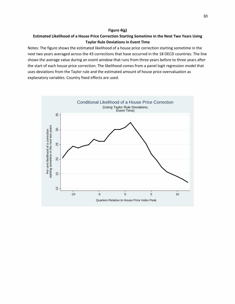
changes in probability of predicting a correction that starts sometime in the next twoyears. The bottom panel of Table 3 provides these estimates. The estimated probabilitiesfrom the base-case model rises by 9.2 per cent during the two-year period leading up tothe start of a correction. They in turn fall by 12.4 per cent during the correction period.Figure 4(g) shows that the probabilities reach approximately 32 per cent on average beforethe start of the corrections.To see how this model would fare historically, we plot the fitted values in Figure 5.

Once again we display the 17-country average using the dark line, with the estimatedvalue for Canada in red. Also shown is the interquartile range across all countries ateach point in time. There are large swings in the 17-country average, with the averageestimated probability peaking at approximately 25 per cent just prior to the onset of theglobal house price crisis of 2007-08. The two previous corrections noted above for Canadaare evident. We note that the estimated likelihood of a correction (i.e., at least a 10 percent decline in real house prices) in the Canadian market that starts sometime in the nexttwo years is approximately 20 per cent.8

4.2 Two components of the long-term interest rate

The forward-looking measure of the monetary policy stance in each of the countries pro-duces a similar outcome. The first columns of Tables 2(a), 2(b), and 2(c) show the abilityof the estimated house price overvaluation and the two components of the long-term in-terest rate to forecast house price corrections that start next quarter, sometime in thenext year and sometime in the next two years, respectively.The estimated coeffi cients on the degree of house price overvaluation are close to their

8The standard errors associated with this in-sample prediction are large, so the 95 per cent confidenceinterval of this estimate ranges from 10 to 30 per cent.

12

values shown in Table 1. They also retain their statistical significance. The expectationscomponent, which represents investors’ forecasts of future policy rates, has strong pre-dictive power for corrections at all forecast horizons. At the quarterly forecast horizon,the coeffi cient is 12.78 and is significant at the 10 per cent level. As the forecast horizonincreases, the coeffi cient increases in size, reaching 19.90 (5 per cent significance) at thetwo-year horizon. As the market increases its assessment of future policy rate increases,the likelihood of a house price correction rises. We note again that this measure is rela-tively forward looking. The event study analysis (Figure 4(e)) shows that this componentincreases in a period that starts three years before the correction, rising by about 100 basispoints. The expectations component remains elevated up to the start of the correction,at which point it rapidly declines.Of interest, the term structure risk premium in each country proves not to be a sta-

tistically significant predictor of house price crises. Indeed the coeffi cient changes sign asthe forecast horizon increases, decreasing from 6.899 at the quarterly horizon to -5.241at a two-year horizon. The coeffi cient is not significant at any horizon. An analysis ofthe risk premium in event time reveals why (Figure 4(f)). While it does display somevariation, the estimated risk premium remains low ahead of the start of the correction.The estimated output gap shows that these are boom times and investor risk aversionis likely to be low. Once the correction has started, the risk premium increases rapidly,rising by over 100 basis points on average, as investors become more risk averse.We can relate this finding to three strands of the existing literature. First, it supports

the analysis found in Bauer and Diez de los Rios (2012) and others, who find that termstructure risk-premiums are strongly countercyclical. The event study here shows that thecountercyclical nature of the term structure risk premium may be related to the housingcycle.Second, the analysis may explain why previous studies that use long-term interest

rates have not found them to be statistically significant predictors of crises or housingmarket cycles (e.g., Kuttner (2012)). The two components of the long-term interest ratemove in opposite directions before and after the start of the house price correction. Theseoffsetting movements would tend to diminish the role of the total long-term interest rateduring these times.Third, the analysis provides support for those who advocate using risk premiums to

provide an assessment for financial stability (e.g., Stein (2014)). Here the risk premiumsare used to obtain a better measure of investor expectations of future policy rates. Theseexpectations increase long before the beginning of the house price correction and remainelevated. It may be, however, that more advanced techniques could capture the “low forlong”aspect of the risk premiums themselves and use this as a predictor of house pricecorrections and other phenomena of interest.Once again we may use the statistical criteria to evaluate the in-sample fit of the

model. The pseudo-R2 statistics are similar in value to those from the Taylor rule model.The estimated hit rate remains relatively flat, rising from 71.2 per cent at the quarterlyhorizon to 72.7 per cent at the two-year horizon. The QPS statistic rises moderatelywith the forecast horizon from 0.027 for one quarter ahead to 0.155 for two years ahead.While this would indicate a deterioration in forecast performance, the difference between

13

this statistic and the unconditional measure (9) actually improves. In addition, the areabeneath the ROC curve increases from 0.828 to 0.864. Thus, there are moderate increasesin forecast accuracy using the statistical metrics.As above, an examination of the trend of the probabilities around the corrections

reveals a better way to interpret the model results. The top panel of Table 4 shows thechange in probabilities of a house price correction starting in the next quarter, during atwo-year event window on both sides of the start of the correction. The results show thatthe estimated probability of a crisis over the next quarter increases by 1.6 per cent over atwo-year window prior to the crisis. Although this is statistically significant it would bediffi cult for policy-makers to rely on such a small degree of variation to change policiesto avoid a crisis. The quarterly probabilities decrease by 2.1 per cent in the two-yearperiod after the crisis. Thus, the average difference in probabilities between the pre- andpost-crisis periods is 3.8 per cent, which is statistically significant with a P -value <0.001.In contrast, it is much easier to notice the changes in probabilities as the associated

forecast horizon lengthens. When the probabilities are calculated for a two-year horizon,they increase by a total of 9.2 per cent (statistically significant) in the two-year periodprior to the crisis. Once the crisis has arrived, the probabilities decline by 16.1 per cent,resulting in a statistically significant difference of 25.3 per cent in the two-year windowspre- and post-crisis. Such a stronger signal would be easier for policy-makers to interpret.These results mirror those for the model that uses the Taylor rule deviation.We can put the current likelihood of a house price correction into context by examining

the likelihood of a crash around the 43 correction “events”that were shown in Figure 1.Figure 4(h) shows an event study of the likelihood of a correction starting sometime inthe next two years. The slow increase in the likelihood of a crisis matches that of theTaylor rule model. Table 4 shows that the increase in probabilities at the three horizonsis similar to their Taylor rule counterparts.

4.3 Credit measures as predictors

As mentioned in the introduction, a number of papers have used measures of creditto forecast banking, credit and foreign exchange crises. Here we assess their ability toimprove the models used to forecast house price corrections. As mentioned above, wehave normalized the two credit series (total and bank) by both the consumer price indexand by the level of GDP. We include four lags (i.e., one year) of the series to examine anychanges in the dynamics.The second and third columns of Table 1 show the coeffi cients on the real total and

bank credit series, respectively, in the panel logit regression model that includes the Taylorrule deviation as a predictor. It is interesting to note that coeffi cients on the real creditseries increase in size and significance as the forecast horizon increases. Indeed, all ofthe coeffi cients are individually significant in the model that assesses the likelihood of acorrection starting sometime in the next two years (Table 1(c)). The coeffi cients are allpositive, indicating that an increase in credit to the non-financial private sector aids inthe forecasts of corrections. Without further structure, however, it is not clear why theseries have this effect. It could be that homeowners become overextended so that thedemand for credit must decline in the correction period. It could also be that lenders

14

change the desire to supply credit as they anticipate a downturn in the economy. We notethat the coeffi cient attached to the Taylor rule deviation becomes insignificant when thereal credit series are included.The fourth and fifth columns of Table 1 show the coeffi cients on the credit series nor-

malized by GDP. These variables are not statistically significant predictors of correctionsat any of the horizons examined.The real credit series also enter significantly when the two components of the long-

term interest rate are used as predictors, especially at the two-year horizon (second andthird columns of Table 2). In contrast to the Taylor rule specification, the forward-looking measure of policy interest rates (the expectations component) remains statisticallysignificant at all horizons. The term premium remains insignificant.While the real credit series are statistically significant predictors, they do not appear

to improve the in-sample fit of the model by a large amount. Focusing on the two-yearhorizon for the model in Table 2(c), we see that the hit rates actually decrease when thereal credit variables are included. However, the other statistics show a small improvementover the base-case model. The QPS test statistic (8) is smaller and the difference betweenthe QPS statistics for this model and the unconditional one (9) becomes more negative.The AUROC statistics rise slightly.While the coeffi cients are statistically significant and some of the statistics indicate

a better in-sample fit, it is not certain that the dynamics of total real credit would aidpolicy-makers in this application. The bottom panel of Table 4 shows that the estimatedlikelihood of a correction would increase by 10.8 per cent in the two-year period prior tothe start of the correction. This is only a small gain compared to the 9.2 per cent increasedisplayed by the base-case model with the two components of the long-term interest rate.

5 Final Remarks

In this paper, we construct a panel logit regression model that attempts to forecast houseprice corrections in 18 OECD countries. The model incorporates a simple measure ofthe overvaluation of the houses in each country along with two different estimates ofthe monetary policy stance of the central bank in each country. We also include somemeasures of the quantity of credit that have been recently issued in each country.There are a number of conclusions of interest to policy-makers. First, the relatively

simple way of assessing house price overvaluation has good forecasting power for sub-sequent corrections. The variable is significant in all specifications and at all horizons.Second, while the two methods of estimating the monetary policy stance of the centralbanks produce similar results, the method of extracting a global risk premium from thelong-term interest rate has some advantages. The expectations component is forwardlooking and rises well in advance of the corrections. This may be quite useful to policy-makers today who face the zero lower bound on current policy rates while the long-termrates incorporate expectations of future rate increases.Third, there is a distinct forecast-horizon aspect to the results. Attempting to forecast

a house price decline that is going to start in the next quarter is extremely diffi cult. Thesignals from this modelling approach are very weak and would be engulfed by the noise

15

of the estimates. In contrast, when we construct the likelihood of a correction occurringsometime in the next two years, the method produces clearer results. The increase inthe estimated probability of the corrections is much larger. We note again that suchlikelihoods will always remain diffi cult to interpret, since values near zero or one areunlikely to occur.Finally, this paper provides evidence that price measures forecast house price correc-

tions better than measures of the quantity of credit. While the latter have proved quitepopular in forecasting a variety of crises, it would be interesting to see whether price-basedmeasures would be helpful in that regard as well.

16

References

[1] Agnello, L. and L. Schuknecht. 2011. “Booms and Busts in Housing Markets: Deter-minants and Implications,”Journal of Housing Economics 20, pp.171-190.

[2] Ahearne, A.G., J. Ammer, B.M. Doyle, L.S. Kole, and R.F. Martin. 2005. “HousePrices and Monetary Policy: A Cross-Country Study,”Board of Governors of theFederal Reserve System, International Finance Discussion Paper 841.

[3] Alpanda, S. and S. Zubairy. 2013. “Housing and Tax Policy,”Bank of Canada workingpaper 2013-33.

[4] Baron, M. and W. Xiong. 2014. “Credit Expansions and Neglected Crash Risk.”Princeton University working paper.

[5] Bauer, G.H. and A. Diez de los Rios. 2012. “An International Dynamic Term Struc-ture Model with Economic Restrictions and Unspanned Risks.” Bank of Canadaworking paper 2012-5.

[6] Bordo, M.D. and J.L. Lane. 2013. “Does Expansionary Monetary Policy Cause AssetPrice Booms; Some Historical and Empirical Evidence,”NBER working paper seriesno. 19585.

[7] Campbell, S.D., M.A. Davis, J. Gallin, and R.F. Martin. 2009. “What Moves HousingMarkets: A Variance Decomposition of the Rent-Price Ratio,” Journal of UrbanEconomics, vol. 66, no. 2, pp. 90-102.

[8] Campbell, J.Y., J. Hilscher, and J. Szilagyi. 2008. “In Search of Distress Risk,”Journal of Finance vol. 58, no. 6, pp. 2899-2939.

[9] Croce, R.M., and D.R. Haurin. 2009. “Predicting Turning Points in the HousingMarket,”Journal of Housing Economics 18, pp.281-293.

[10] Davis, M.A. and S. Van Nieuwerburgh. 2014. “Housing, Finance and the Macroecon-omy.”Department of Real Estate, University of Wisconsin-Madison working paper.

[11] Diebold, F.X. and R.S. Mariano. 1995. “Comparing Predictive Accuracy,” Journalof Business and Economic Statistics 13, pp. 253-263.

[12] Dynan, K.E. and D.L. Kohn. 2007. “The Rise in U.S. Household Indebtedness:Causes and Consequences,”Federal Reserve Board Finance and Economics Discus-sion Series 2007-37.

[13] Eickmeier, S., and B. Hofmann. 2013. “Monetary Policy, Housing Booms and Finan-cial (Im)balances,”Macroeconomic Dynamics 17, pp. 830-860.

[14] Glaeser, E.L., J.D. Gottlieb and J. Gyourko. 2010. “Can Cheap Credit Explain theHousing Boom,”NBER working paper series no. 16230.

17

[15] Glaeser, E.L. and C.G. Nathanson. 2014. “Housing Bubbles.”NBER working paper20426.

[16] Gourinchas, P.O. and M. Obstfeld. 2012. “Stories of the Twentieth Century for theTwenty-First,”American Economic Journal: Macroeconomics 4, pp. 226-265.

[17] Harding, D. and A. Pagan. 2002. “Dissecting the cycle: a methodological investiga-tion,”Journal of Monetary Economics 49, pp. 365-381.

[18] Iacoviello, M. 2005. “House Prices, Borrowing Constraints and Monetary Policy inthe Business Cycle,”American Economic Review, pp. 739-764.

[19] Iacoviello, M. and S. Neri. 2010. “Housing Market Spillovers: Evidence from anEstimated DSGE Model,”American Economic Journal : Macroeconomics 2, April2010, 125-164.

[20] Igan, D. and P. Loungani. 2012. “Global Housing Cycles,” IMF Working PaperWP/12/17.

[21] Jarocinski, M. and F.R. Smets. 2008. “House Prices and the Stance of MonetaryPolicy,”Federal Reserve Bank of St. Louis Review, July/August, pp. 339-365.

[22] Jorda, O., M. Schularick and A.M. Taylor. 2013. “When Credit Bites Back.”Journalof Money, Credit and Banking, vol. 45, no. 2, pp. 3-28.

[23] Jorda, O., M. Schularick and A.M. Taylor. 2014a. “Financial Crises, Credit Boomsand External Imbalances: 140 Years of Lessons.” IMF Economic Review, June 2011,59(2): 340-378

[24] Jorda, O., M. Schularick and A.M. Taylor. 2014b. “Betting the House.” FederalReserve Bank of San Francisco working paper.

[25] Kuttner, K.N. 2012. “Low Interest Rates and Housing Bubbles: Still No SmokingGun,”working paper, William College.

[26] Ludvigson, S.C. 2007. “Discussion of Housing and Consumer Behavior.”Proceedingsof the Federal Reserve Bank of Kansas City’s symposium on “Housing, HousingFinance, and Monetary Policy,”Jackson Hole, Wyoming.

[27] Peterson, B. 2012. “Fooled by Search: Housing Prices, Turnover and Bubbles.”Bankof Canada working paper 2012-3.

[28] Peterson, B. and Y. Zheng. 2011. “Medium-Term Fluctuations in Canadian HousePrices.”Bank of Canada Review, Winter 2011-12.

[29] Schembri, L. 2014. “Housing Finance in Canada: Looking Back to Move Forward.”National Institute Economic Review (November): R45-R57.

[30] Schularick, M. and A. M. Taylor. 2012. “Credit Booms Gone Bust: Monetary Policy,Leverage Cycles, and Financial Crises, 1870-2008,”American Economic Review 102pp. 1029-61.

18

[31] Stein, J.C. 2014. “Incorporating Financial Stability Considerations into a MonetaryPolicy Framework.”Board of Governors of the Federal Reserve System, WashingtonD.C.

[32] Taylor, J.B. 2007. “Housing and Monetary Policy,”NBER working paper series no.13682.

[33] Thompson, S.B. 2011. “Simple Formulas for Standard Errors that Cluster by bothFirm and Time.”Journal of Financial Economics 99, 1-10.

19

20

Figure 1 Start of House Price Corrections

Notes: the figure shows the start dates of the 43 housing market corrections (a decline in real house prices of at least 10 per cent that lasts at least four quarters) in all 18 OECD countries from 1975Q1 to 2014Q2. The corrections for Canada are displayed in red.

01

23

4

Num

ber o

f Cor

rect

ions

1975

q1

1977

q1

1979

q1

1981

q1

1983

q1

1985

q1

1987

q1

1989

q1

1991

q1

1993

q1

1995

q1

1997

q1

1999

q1

2001

q1

2003

q1

2005

q1

2007

q1

2009

q1

2011

q1

2013

q1

2015

q1

Date

All Other Countries Canada

Housing Market Corrections for 18 OECD Countries

21

33.

54

4.5

55.

5

1975 1980 1985 1990 1995 2000 2005 2010 2015

Australia

33.

54

4.5

55.

5

1975 1980 1985 1990 1995 2000 2005 2010 2015

Belgium

33.

54

4.5

55.

5

1975 1980 1985 1990 1995 2000 2005 2010 2015

Canada

33.

54

4.5

55.

5

1975 1980 1985 1990 1995 2000 2005 2010 2015

Denmark

33.

54

4.5

55.

5

1975 1980 1985 1990 1995 2000 2005 2010 2015

Spain

33.

54

4.5

55.

5

1975 1980 1985 1990 1995 2000 2005 2010 2015

Finland

33.

54

4.5

55.

5

1975 1980 1985 1990 1995 2000 2005 2010 2015

France

33.

54

4.5

55.

5

1975 1980 1985 1990 1995 2000 2005 2010 2015

United Kingdom

33.

54

4.5

55.

5

1975 1980 1985 1990 1995 2000 2005 2010 2015

Germany

Figure 2 Duration of House Price Corrections

Notes: The figure shows the log real house price index and the housing market corrections (a decline in real house prices of at least 10 per cent that lasts at least four quarters) in all 18 OECD countries from 1975Q1 to 2014Q2.

22

33.

54

4.5

55.

5

1975 1980 1985 1990 1995 2000 2005 2010 2015

Ireland

33.

54

4.5

55.

5

1975 1980 1985 1990 1995 2000 2005 2010 2015

Italy

33.

54

4.5

55.

5

1975 1980 1985 1990 1995 2000 2005 2010 2015

Japan

33.

54

4.5

55.

5

1975 1980 1985 1990 1995 2000 2005 2010 2015

Netherlands3

3.5

44.

55

5.5

1975 1980 1985 1990 1995 2000 2005 2010 2015

Norway

33.

54

4.5

55.

5

1975 1980 1985 1990 1995 2000 2005 2010 2015

New Zealand

33.

54

4.5

55.

5

1975 1980 1985 1990 1995 2000 2005 2010 2015

Switzerland

33.

54

4.5

55.

5

1975 1980 1985 1990 1995 2000 2005 2010 2015

Sweden

33.

54

4.5

55.

5

1975 1980 1985 1990 1995 2000 2005 2010 2015

United States

Figure 2, continued House Price Corrections

23

Figure 3 Estimated Level of House Price Overvaluation

Notes: The figure shows the estimated level of house price overvaluation for Canada (red line) and the average value of the 17 other OECD countries (black line). Also shown is the interquartile range (the 25th and 75th highest amounts of overvaluation across all 18 countries at each point in time) in dotted lines. The fundamental value of the house price index comes from a panel regression model where the real house price index is regressed on real, per capita disposable income and the long-term government bond yield in each country. The estimated degree of overvaluation is the residual from the regression. Country fixed effects are used.

-40

-20

020

40

Per

cen

t dev

iatio

n fro

m m

odel

val

ue

1975q1 1980q1 1985q1 1990q1 1995q1 2000q1 2005q1 2010q1 2015q1

Date

All Other Country Average CanadaInterquartile Range (All Countries)

House Price Overvaluation

24

Figure 4(a) Estimated Level of House Price Overvaluation in Event Time

Notes: The figure shows the estimated level of house price overvaluation averaged across the 43 corrections that have occurred in the 18 OECD countries. The line shows the average value during an event window that runs from three years before to three years after the start of each house price correction. The fundamental value of the house price index comes from a panel regression model where the real house price index is regressed on real, per capita disposable income and the long-term government bond yield. Country fixed effects are used. The estimated amount of overvaluation is the residual from the panel regression.

05

1015

20

Per

cen

t dev

iatio

n fro

m m

odel

val

ue

-10 -5 0 5 10

Quarters Relative to House Price Index Peak

(Event Time)House Price Overvaluation

25

Figure 4(b) Estimated Output Gap in Event Time

Notes: The figure shows the estimated level of the output gap averaged across the 43 corrections that have occurred in the 18 OECD countries. The line shows the average value during an event window that runs from three years before to three years after the start of each house price correction. The output gap is the difference between the actual level of real, per capita disposable income and the value estimated from a Hodrick-Prescott filtered value with a smoothing coefficient of 1600.

-.50

.51

1.5

Per

cen

t

-10 -5 0 5 10


(Event Time)Output Gap

26

Figure 4(c) Estimated Inflation Gap in Event Time

Notes: The figure shows the estimated level of the inflation gap averaged across the 43 corrections that have occurred in the 18 OECD countries. The line shows the average value during an event window that runs from three years before to three years after the start of each house price correction. The gap is the difference between the actual level of inflation and a target level. Prior to 1995, the target level of inflation is set equal to the previous quarter’s inflation rate times 0.95. After 1995, the target level is set equal to 2 per cent in each country.

-.50

.51

Per

cen

t

-10 -5 0 5 10


(Event Time)Inflation Gap

27

Figure 4(d) Estimated Deviation from the Taylor Rule in Event Time

Notes: The figure shows the estimated level of the deviation from the Taylor rule averaged across the 43 corrections that have occurred in the 18 OECD countries. The line shows the average value during an event window that runs from three years before to three years after the start of each house price correction. The estimated Taylor rule level of the interest rate is a weighted combination of the output and inflation gaps as described in the text. The deviation is the difference between the actual short-term interest rate and the estimated Taylor rule rate.

0.2

.4.6

.8

Per

cen

t

-10 -5 0 5 10


(Event Time)Deviation from Taylor Rule

28

Figure 4(e) Estimated Expectations Component of the Long-Term Interest Rate in Event Time

Notes: The figure shows the estimated level of the expectations component of the long-term interest rate averaged across the 43 corrections that have occurred in the 18 OECD countries. The line shows the average value during an event window that runs from three years before to three years after the start of each house price correction. The expectations component is the residual from a projection of the long-term interest rate in each country on the estimated U.S. term structure risk premium from Bauer and Diez de los Rios (2012).

.51

1.5

22.

5

Per

cen

t

-10 -5 0 5 10


(Event Time)Expectations Component of the Long-Term (10-Year) Interest Rate

29

Figure 4(f) Estimated Term Premium Component of the Long-Term Interest Rates in Event Time

Notes: The figure shows the estimated level of the term premium component of the long-term interest rate averaged across the 43 corrections that have occurred in the 18 OECD countries. The line shows the average value during an event window that runs from three years before to three years after the start of each house price correction. The term premium component for each country is estimated by projecting the long-term interest rate on the U.S. term structure risk premium from Bauer and Diez de los Rios (2012).

66.

57

7.5

8

Per

cen

t

-10 -5 0 5 10


(Event Time)Term Premium Component of the Long-Term (10-Year) Interest Rate

30

Figure 4(g) Estimated Likelihood of a House Price Correction Starting Sometime in the Next Two Years Using

Taylor Rule Deviations in Event Time Notes: The figure shows the estimated likelihood of a house price correction starting sometime in the next two years averaged across the 43 corrections that have occurred in the 18 OECD countries. The line shows the average value during an event window that runs from three years before to three years after the start of each house price correction. The likelihood comes from a panel logit regression model that uses deviations from the Taylor rule and the estimated amount of house price overvaluation as explanatory variables. Country fixed effects are used.

1015

2025

3035

Per

cen

t lik

elih

ood

of a

cor

rect

ion

star

ting

som

etim

e in

the

next

two

year

s

-10 -5 0 5 10


(Using Taylor Rule Deviations,Event Time)

Conditional Likelihood of a House Price Correction

31

Figure 4(h) Estimated Likelihood of a House Price Correction Starting Sometime in the Next Two Years Using the

Two Components of the Long-Run Interest Rates in Event Time Notes: The figure shows the estimated likelihood of a house price correction starting sometime in the next two years averaged across the 43 corrections that have occurred in the 18 OECD countries. The line shows the average value during an event window that runs from three years before to three years after the start of each house price correction. The likelihood comes from a panel logit regression model that uses the two components of the long-term interest rate and the estimated amount of house price overvaluation as explanatory variables. Country fixed effects are used.

1015

2025

3035

Per

cen

t lik

elih

ood

of a

cor

rect

ion

star

ting

som

etim

e in

the

next

two

year

s

-10 -5 0 5 10


(Using the Two Components of the Long-Term Interest Rate,Event Time)


32

Figure 5 Estimated Likelihood of a House Price Correction Starting Sometime in the Next Two Years Using

Taylor Rule Deviations Notes: The figure shows the estimated likelihood of a house price correction starting sometime in the next two years for Canada (red line) and the average value of the 17 other OECD countries (black line). Also shown is the interquartile range (the 25th and 75th highest levels of likelihood across all 18 countries at each point in time) in dotted lines. The likelihood comes from a panel logit regression model that uses deviations from the Taylor rule and the estimated amount of house price overvaluation as explanatory variables. Country fixed effects are used.

010

2030

4050

Per

cen

t lik

elih

ood

of a

cor

rect

ion

star

ting

som

etim

e in

the

next

two

year

s

1975q1 1980q1 1985q1 1990q1 1995q1 2000q1 2005q1 2010q1 2015q1

Date


(Baseline Prediction Model Using Taylor Rule Deviations,Country FE Logit)


33

Figure 6 Estimated Likelihood of a House Price Correction Starting Sometime in the Next Two Years Using the

Two Components of the Long-Tun Interest Rate Notes: The figure shows the estimated likelihood of a house price correction starting sometime in the next two years for Canada (red line) and the average value of the 17 other OECD countries (black line). Also shown is the interquartile range (the 25th and 75th highest levels of likelihood across all 18 countries at each point in time) in dotted lines. The likelihood comes from a panel logit regression model that uses the two components of the long-term interest rate and the estimated amount of house price overvaluation as explanatory variables. Country fixed effects are used.

020

4060

Per

cen

t lik

elih

ood

of a

cor

rect

ion

star

ting

som

etim

e in

the

next

two

year

s

1975q1 1980q1 1985q1 1990q1 1995q1 2000q1 2005q1 2010q1 2015q1

Date


(Baseline Prediction Model Using the Two Components of the Long-Term Interest Rate,Country FE Logit)


34

Table 1(a) Results of Panel Logit Regression Models Using Deviations from the Taylor Rule to Evaluate the Likelihood

of a House Price Correction Starting in the Next Quarter Notes: The table shows the estimated coefficients and summary statistics from the panel logit regression models that evaluate the likelihood of a house price correction starting in the next quarter. The models use the estimated amount of house price overvaluation (ƐHP) and the deviation of the short-term interest rate from its Taylor rule level (ƐTR) as an estimate of the monetary policy stance of the central bank. Other measures of credit are then added as regressors. Country fixed effects (parameters not shown) are used. The standard errors shown in round brackets are robust to clustering at both the country level and over time (Thompson 2011). The starts indicate marginal significance levels (*** P<0.01, ** P<0.05, * P<0.1). The summary statistics are explained in the text.

Base case

Base case + Total (real)

credit (all)


credit (banks)

Base case + Total

credit/GDP (all)

Base case + Total

credit/GDP (banks)

ƐHP 5.988*** 5.747*** 5.550*** 5.970*** 5.767***

(1.117) (0.967) (0.886) (1.113) (1.027)

ƐTR 11.00** 7.493 8.343 10.77** 10.24*

(5.299) (5.400) (5.303) (5.351) (5.254)

Δtcredt-1

-3.703

(10.69)

Δtcredt-2

2.229

(12.65)

Δtcredt-3

5.217

(9.782)

Δtcredt-4

23.24*

(13.31)

Δbcredt-1

0.629

(12.54)

Δbcredt-2

-0.592

(11.47)

Δbcredt-3

3.483

(11.47)

Δbcredt-4

13.45

(9.078)

Δtcred/GDPt-1

0.340*

(0.177)

Δtcred/GDPt-2

0.303

(0.225)

Δtcred/GDPt-3

0.223

(0.148)

Δtcred/GDPt-4

0.440**

(0.182)

Δbcred/GDPt-1

0.384**

(0.164)

Δbcred/GDPt-2

0.222

(0.242)

Δbcred/GDPt-3

0.277*

(0.162)

Δbcred/GDPt-4

0.395** (0.195)

35

Observations 2,719 2,667 2,567 2,667 2,567 Pseudo R2 0.218 0.234 0.245 0.219 0.239

Chi-sq. stat. 39.016 8.119 4.299 6.768 6.754 P-value 0.000 0.001 0.065 0.000 0.079

Hit rate 0.691 0.680 0.653 0.671 0.642 (s.e.) (0.016) (0.034) (0.006) (0.016) (0.004)

QPS stat. 0.026 0.026 0.025 0.027 0.026 (s.e.) (0.003) (0.008) (0.006) (0.033) (0.033)

QPS diff. stat. -0.001 -0.001 -0.001 -0.001 -0.001 (s.e.) (0.000) (0.009) (0.000) (0.004) (0.000) P-value 0.105 0.040 0.367 0.111 0.001

AUROC 0.822 0.814 0.812 0.820 0.815 (s.e.) (0.032) (0.001) (0.003) (0.004) (0.004) Chi-sq. test 13.223 11.525 11.086 12.973 12.047 P-value 0.000 0.000 0.001 0.000 0.001

36

Table 1(b) Results of Panel Logit Regression Models Using Deviations from the Taylor Rule to Evaluate the Likelihood of

a House Price Correction Starting Sometime in the Next Year Notes: The table shows the estimated coefficients and summary statistics from the panel logit regression models that evaluate the likelihood of a house price correction starting sometime in the next year. The models use the estimated amount of house price overvaluation (ƐHP) and the deviation of the short-term interest rate from its Taylor rule level (ƐTR) as an estimate of the monetary policy stance of the central bank. Other measures of credit are then added as regressors. Country fixed effects (parameters not shown) are used. The standard errors shown in round brackets are robust to clustering at both the country level and over time (Thompson 2011). The starts indicate marginal significance levels (*** P<0.01, ** P<0.05, * P<0.1). The summary statistics are explained in the text.

(1) (2) (3) (4) (5)

Base case


credit (all)


credit (banks)

Base case + Total

credit/GDP (all)

Base case + Total

credit/GDP (banks)

ƐHP 6.737*** 6.440*** 6.176*** 6.717*** 6.483***

(1.090) (0.991) (0.918) (1.085) (1.018)

ƐTR 14.81*** 10.45 10.81* 14.60*** 13.84**

(5.552) (6.732) (6.406) (5.647) (5.555)

Δtcredt-1

6.592

(5.323)

Δtcredt-2

6.738

(4.829)

Δtcredt-3

13.69***

(4.072)

Δtcredt-4

9.838**

(4.551)

Δbcredt-1

4.195

(4.416)

Δbcredt-2

3.652

(3.893)

Δbcredt-3

9.939***

(3.256)

Δbcredt-4

7.994

(5.428)

Δtcred/GDPt-1

0.370**

(0.172)

Δtcred/GDPt-2

0.355**

(0.159)

Δtcred/GDPt-3

0.381**

(0.152)

Δtcred/GDPt-4

0.313*

(0.173)

Δbcred/GDPt-1

0.366**

(0.172)

Δbcred/GDPt-2

0.347**

(0.160)

Δbcred/GDPt-3

0.370**

(0.163)

Δbcred/GDPt-4

0.307 (0.188)

37



Hit rate 0.693 0.681 0.654 0.673 0.651 (s.e.) (0.014) (0.003) (0.017) (0.013) (0.017)

QPS stat. 0.090 0.088 0.086 0.091 0.087 (s.e.) (0.006) (0.006) (0.002) (0.002) (0.014)



38

Table 1(c) Results of Panel Logit Regression Models Using Deviations from the Taylor Rule to Evaluate the Likelihood

of a House Price Correction Starting Sometime in the Next Two Years Notes: The table shows the estimated coefficients and summary statistics from the panel logit regression models that evaluate the likelihood of a house price correction starting sometime in the next two years. The models use the estimated amount of house price overvaluation (ƐHP) and the deviation of the short-term interest rate from its Taylor rule level (ƐTR) as an estimate of the monetary policy stance of the central bank. Other measures of credit are then added as regressors. Country fixed effects (parameters not shown) are used. The standard errors shown in round brackets are robust to clustering at both the country level and over time (Thompson 2011). The starts indicate marginal significance levels (*** P<0.01, ** P<0.05, * P<0.1). The summary statistics are explained in the text.

(1) (2) (3) (4) (5)

Base case


credit (all)


credit (banks)

Base case + Total

credit/GDP (all)

Base case + Total

credit/GDP (banks)

ƐHP 6.952*** 6.617*** 6.243*** 6.922*** 6.670***

(1.233) (1.126) (1.044) (1.229) (1.174)

ƐTR 13.99** 8.521 7.903 13.80** 12.91**

(6.360) (7.672) (7.559) (6.442) (6.373)

Δtcredt-1

12.18***

(4.628)

Δtcredt-2

12.02***

(4.604)

Δtcredt-3

12.18**

(5.483)

Δtcredt-4

11.69***

(4.116)

Δbcredt-1

9.647**

(3.815)

Δbcredt-2

9.268***

(3.595)

Δbcredt-3

10.77***

(4.071)

Δbcredt-4

13.05***

(4.361)

Δtcred/GDPt-1

0.372**

(0.187)

Δtcred/GDPt-2

0.348**

(0.176)

Δtcred/GDPt-3

0.334*

(0.172)

Δtcred/GDPt-4

0.281

(0.188)

Δbcred/GDPt-1

0.399**

(0.189)

Δbcred/GDPt-2

0.383**

(0.179)

Δbcred/GDPt-3

0.371**

(0.181)

Δbcred/GDPt-4

0.340* (0.190)

39



Hit rate 0.690 0.695 0.672 0.669 0.650 (s.e.) (0.013) (0.013) (0.031) (0.022) (0.008)

QPS stat. 0.153 0.148 0.143 0.154 0.149 (s.e.) (0.009) (0.031) (0.012) (0.009) (0.013)



40

Table 2(a) Results of Panel Logit Regression Models Using the Two Components of the Long-Term Interest Rate to

Evaluate the Likelihood of a House Price Correction Starting in the Next Quarter Notes: The table shows the estimated coefficients and summary statistics from the panel logit regression models that evaluate the likelihood of a house price correction starting in the next quarter. The models use the estimated amount of house price overvaluation (ƐHP), and the two components of the long-term interest rate (the expectations component (rEC), which acts as a measure of the monetary policy stance of the central bank, and the term premium component (tp)). Other measures of credit are then added as regressors. Country fixed effects (parameters not shown) are used. The standard errors shown in round brackets are robust to clustering at both the country level and over time (Thompson 2011). The starts indicate marginal significance levels (*** P<0.01, ** P<0.05, * P<0.1). The summary statistics are explained in the text.

(1) (2) (3) (4) (5)

Base case


credit (all)


credit (banks)

Base case + Total

credit/GDP (all)

Base case + Total

credit/GDP (banks)

ƐHP 5.335*** 5.285*** 5.075*** 5.487*** 5.290***

(1.387) (1.045) (0.994) (1.377) (1.287)

rEC 12.78* 17.02** 15.57** 13.11* 12.92*

(7.189) (7.121) (6.887) (7.064) (7.108)

tp 6.899 8.411 9.149 7.247 7.426

(7.081) (7.342) (7.035) (6.838) (6.784)

Δtcredt-1

1.824

(10.89)

Δtcredt-2

4.659

(11.00)

Δtcredt-3

9.881

(9.216)

Δtcredt-4

25.75**

(12.49)

Δbcredt-1

4.945

(11.76)

Δbcredt-2

0.675

(10.22)

Δbcredt-3

6.850

(10.39)

Δbcredt-4

16.46*

(8.767)

Δtcred/GDPt-1

0.402**

(0.173)

Δtcred/GDPt-2

0.362*

(0.202)

Δtcred/GDPt-3

0.324**

(0.136)

Δtcred/GDPt-4

0.490***

(0.187)

Δbcred/GDPt-1

0.428***

(0.164)

Δbcred/GDPt-2

0.305

(0.195)

Δbcred/GDPt-3

0.351**

(0.156)

Δbcred/GDPt-4

0.449** (0.192)

41



Hit rate 0.712 0.693 0.660 0.674 0.645 (s.e.) (0.014) (0.019) (0.008) (0.005) (0.017)

QPS stat. 0.027 0.026 0.026 0.027 0.026 (s.e.) (0.003) (0.001) (0.003) (0.004) (0.003)

QPS diff. stat. 0.000 -0.001 -0.001 -0.001 -0.001 (s.e.) (0.000) (0.011) (0.008) (0.005) (0.000) P-value 0.157 0.013 0.056 0.000 0.127


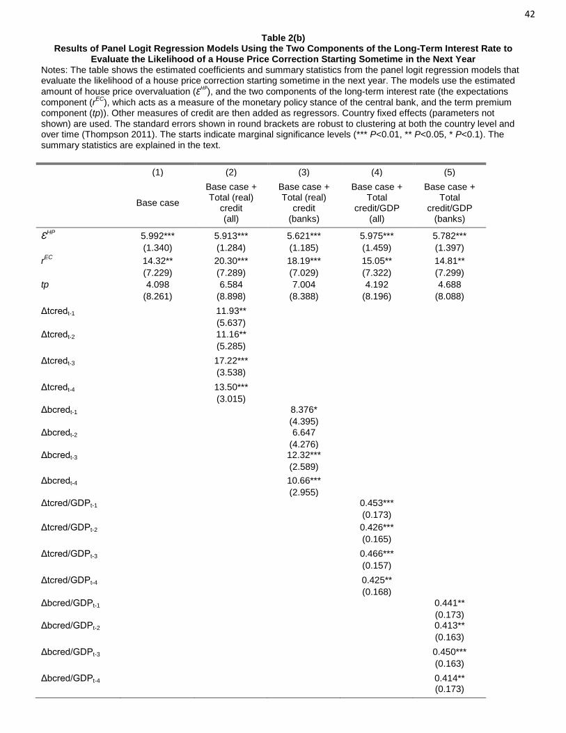
42

Table 2(b) Results of Panel Logit Regression Models Using the Two Components of the Long-Term Interest Rate to

Evaluate the Likelihood of a House Price Correction Starting Sometime in the Next Year Notes: The table shows the estimated coefficients and summary statistics from the panel logit regression models that evaluate the likelihood of a house price correction starting sometime in the next year. The models use the estimated amount of house price overvaluation (ƐHP), and the two components of the long-term interest rate (the expectations component (rEC), which acts as a measure of the monetary policy stance of the central bank, and the term premium component (tp)). Other measures of credit are then added as regressors. Country fixed effects (parameters not shown) are used. The standard errors shown in round brackets are robust to clustering at both the country level and over time (Thompson 2011). The starts indicate marginal significance levels (*** P<0.01, ** P<0.05, * P<0.1). The summary statistics are explained in the text.

(1) (2) (3) (4) (5)

Base case


credit (all)


credit (banks)

Base case + Total

credit/GDP (all)

Base case + Total

credit/GDP (banks)

ƐHP 5.992*** 5.913*** 5.621*** 5.975*** 5.782***

(1.340) (1.284) (1.185) (1.459) (1.397)

rEC 14.32** 20.30*** 18.19*** 15.05** 14.81**

(7.229) (7.289) (7.029) (7.322) (7.299)

tp 4.098 6.584 7.004 4.192 4.688

(8.261) (8.898) (8.388) (8.196) (8.088)

Δtcredt-1

11.93**

(5.637)

Δtcredt-2

11.16**

(5.285)

Δtcredt-3

17.22***

(3.538)

Δtcredt-4

13.50***

(3.015)

Δbcredt-1

8.376*

(4.395)

Δbcredt-2

6.647

(4.276)

Δbcredt-3

12.32***

(2.589)

Δbcredt-4

10.66***

(2.955)

Δtcred/GDPt-1

0.453***

(0.173)

Δtcred/GDPt-2

0.426***

(0.165)

Δtcred/GDPt-3

0.466***

(0.157)

Δtcred/GDPt-4

0.425**

(0.168)

Δbcred/GDPt-1

0.441**

(0.173)

Δbcred/GDPt-2

0.413**

(0.163)

Δbcred/GDPt-3

0.450***

(0.163)

Δbcred/GDPt-4

0.414** (0.173)

43



Hit rate 0.704 0.689 0.662 0.670 0.645 (s.e.) (0.014) (0.017) (0.019) (0.014) (0.019)

QPS stat. 0.093 0.087 0.086 0.093 0.090 (s.e.) (0.006) (0.016) (0.015) (0.006) (0.002)



44

Table 2(c) Results of Panel Logit Regression Models Using the Two Components of the Long-Term Interest Rate to

Evaluate the Likelihood of a House Price Correction Starting Sometime in the Next Two Years Notes: The table shows the estimated coefficients and summary statistics from the panel logit regression models that evaluate the likelihood of a house price correction starting sometime in the next two years. The models use the estimated amount of house price overvaluation (ƐHP), and the two components of the long-term interest rate (the expectations component (rEC), which acts as a measure of the monetary policy stance of the central bank, and the term premium component (tp)). Other measures of credit are then added as regressors. Country fixed effects (parameters not shown) are used. The standard errors shown in round brackets are robust to clustering at both the country level and over time (Thompson 2011). The starts indicate marginal significance levels (*** P<0.01, ** P<0.05, * P<0.1). The summary statistics are explained in the text.

(1) (2) (3) (4) (5)

Base case


credit (all)


credit (banks)

Base case + Total

credit/GDP (all)

Base case + Total

credit/GDP (banks)

ƐHP 6.201*** 6.172*** 5.835*** 6.285*** 6.080***

(1.297) (1.324) (1.214) (1.377) (1.333)

rEC 19.90** 26.39*** 24.59*** 21.18** 20.72**

(8.094) (8.515) (8.180) (8.346) (8.270)

tp -5.241 -2.330 -1.475 -5.058 -4.285

(9.612) (10.29) (9.853) (9.512) (9.365)

Δtcredt-1

16.96***

(4.441)

Δtcredt-2

15.83***

(4.546)

Δtcredt-3

15.56***

(5.089)

Δtcredt-4

15.07***

(3.896)

Δbcredt-1

13.76***

(3.524)

Δbcredt-2

11.83***

(3.384)

Δbcredt-3

12.25***

(3.377)

Δbcredt-4

14.71***

(2.872)

Δtcred/GDPt-1

0.473**

(0.190)

Δtcred/GDPt-2

0.449**

(0.183)

Δtcred/GDPt-3

0.466***

(0.178)

Δtcred/GDPt-4

0.434**

(0.186)

Δbcred/GDPt-1

0.486**

(0.191)

Δbcred/GDPt-2

0.467**

(0.185)

Δbcred/GDPt-3

0.480***

(0.185)

Δbcred/GDPt-4

0.463** (0.190)

45 Observations 2,808 2,680 2,580 2,684 2,584

Pseudo R2 0.215 0.292 0.307 0.241 0.259


Hit rate 0.727 0.715 0.694 0.699 0.674 (s.e.) (0.013) (0.016) (0.010) (0.016) (0.004)

QPS stat. 0.155 0.142 0.139 0.156 0.150 (s.e.) (0.009) (0.041) (0.008) (0.038) (0.010)



46

Table 3 Average Change in Probability of House Price Correction Using Taylor Rule Deviations and other

Explanatory Variables during Pre- and Post-Correction Periods

Note: The table shows the average change in probability during a two-year window prior to the start of the house price correction (“pre-correction average”) and during the two-year period following the start of the correction (“post-correction average”). Also shown is the average difference between the two periods along with the marginal significance level of a statistical test of the difference (“P-value”). The probabilities are the fitted values from the panel logit models shown in Table 1 that use the estimated deviation of the Taylor rule as a measure of the monetary policy stance of the central banks. The logit models probabilities are calculated for three forecast horizons: house price corrections starting next quarter, house price corrections starting sometime in the next year and house price corrections starting sometime in the next two years. The standard errors shown in round brackets are robust to clustering at both the country level and over time (Thompson 2011).

(1) (2) (3) (4) (5)

Base case


credit (all)


credit (banks)

Base case + Total

credit/GDP (all)

Base case + Total

credit/GDP (banks)

One Quarter

Pre-correction average 0.017 0.022 0.017 0.017 0.016 (s.e.) (0.004) (0.017) (0.033) (0.004) (0.015) Post-correction average -0.018 -0.035 -0.024 -0.018 -0.017 (s.e.) (0.004) (0.034) (0.003) (0.000) (0.033) Difference -0.035 -0.057 -0.041 -0.035 -0.034 (s.e.) (0.004) (0.008) (0.006) (0.004) (0.004) P-value 0.0001 0.001 0.367 0.111 0.079

One Year Pre-correction average 0.064 0.075 0.058 0.064 0.061 (s.e.) (0.013) (0.018) (0.005) (0.013) (0.013) Post-correction average -0.070 -0.107 -0.094 -0.072 -0.068 (s.e.) (0.013) (0.017) (0.016) (0.006) (0.013) Difference -0.134 -0.182 -0.152 -0.136 -0.129 (s.e.) (0.013) (0.020) (0.014) (0.017) (0.005) P-value 0.000 0.000 0.000 0.071 0.000

Two Years Pre-correction average 0.092 0.086 0.056 0.092 0.087 (s.e.) (0.021) (0.009) (0.008) (0.004) (0.012) Post-correction average -0.124 -0.193 -0.183 -0.127 -0.120 (s.e.) (0.022) (0.031) (0.031) (0.014) (0.022) Difference -0.216 -0.279 -0.239 -0.218 -0.207 (s.e.) (0.022) (0.028) (0.012) (0.013) (0.003) P-value 0.000 0.031 0.000 0.000 0.000

47

Table 4 Average Change in Probability of House Price Correction Using the Two Components of the Long-Term

Interest Rate and other Explanatory Variables during Pre- and Post-Correction Periods Note: The table shows the average change in probability during a two-year window prior to the start of the house price correction (“pre-correction average”) and during the two-year period following the start of the correction (“post-correction average”). Also shown is the average difference between the two periods along with the marginal significance level of a statistical test of the difference (“P-value”). The probabilities are the fitted values from the panel logit models shown in Table 2 that use the two components of the long-term interest rate as a measure of the monetary policy stance of the central banks. The logit models probabilities are calculated for three forecast horizons: house price corrections starting next quarter, house price corrections starting sometime in the next year and house price corrections starting sometime in the next two years. The standard errors shown in round brackets are robust to clustering at both the country level and over time (Thompson 2011).

(1) (2) (3) (4) (5)

Base case


credit (all)


credit (banks)

Base case + Total

credit/GDP (all)

Base case + Total

credit/GDP (banks)

One Quarter

Pre-correction average 0.016 0.029 0.019 0.016 0.016 (s.e.) (0.005) (0.032) (0.008) (0.030) (0.005) Post-correction average -0.021 -0.045 -0.032 -0.022 -0.021 (s.e.) (0.004) (0.012) (0.000) (0.000) (0.005) Difference -0.038 -0.074 -0.052 -0.038 -0.037 (s.e.) (0.004) (0.011) (0.016) (0.005) (0.005) P-value 0.000 0.018 0.000 0.097 0.101

One Year Pre-correction average 0.061 0.093 0.065 0.062 0.060 (s.e.) (0.018) (0.006) (0.016) (0.016) (0.006) Post-correction average -0.085 -0.145 -0.121 -0.086 -0.082 (s.e.) (0.015) (0.022) (0.028) (0.016) (0.015) Difference -0.146 -0.238 -0.186 -0.147 -0.142 (s.e.) (0.015) (0.022) (0.019) (0.003) (0.016) P-value 0.000 0.000 0.000 0.009 0.033

Two Years Pre-correction average 0.092 0.108 0.070 0.096 0.093 (s.e.) (0.036) (0.041) (0.052) (0.036) (0.035) Post-correction average -0.161 -0.267 -0.238 -0.170 -0.162 (s.e.) (0.032) (0.011) (0.039) (0.009) (0.038) Difference -0.253 -0.375 -0.308 -0.266 -0.256 (s.e.) (0.032) (0.048) (0.014) (0.010) (0.009) P-value 0.000 0.000 0.000 0.045 0.000

Documents

International House Price Cycles, Monetary Policy and … · International House Price Cycles, Monetary Policy and Risk Premiums . by Gregory H. Bauer . 2 . ... A case study based