Interim Report for Tasks 4.3 and 4.5: Optimal Rate Designs and ISO

Services for Maximizing the Value of Combined PV and Storage

Michael A. Cohen, Joshua A. Taylor and Duncan S. Callaway

University of California, Berkeley

February 27, 2011

This is one of three interim reports completed by a UC Berkeley team of students and faculty in theEnergy and Resources Group. The overall objective of the project is to determine the impact andvalue of coupling distributed storage with photovoltaic systems. Our specific focus is on understanddistribution system impacts and the opportunity for creating value by incorporating storage into theCAISO’s dispatch process.

The tasks of the project are

• 4.2 PV Variability Analysis

• 4.3 - CPP Tariff

• 4.4 - Aggregate control

• 4.5 - CAISO Product

This particular interim report describes our research results and future plans for two tasks:

• Subtask 4.3: Identify the optimal Critical Peak Pricing rate plan. Part I of this report explains thecurrent status of our research. We have focused on understanding the impact of PV and storageon the cost to operate distribution systems.

• Subtask 4.5: Propose a CAISO wholesale market product for FirmPV benefits. Part II of this reportdescribes our work to understand CAISO’s proposed regulation energy management product andpotential alternatives.

Part I

Understanding Distribution System Impacts

1 Introduction

The introduction of large amounts of grid-connected intermittent distributed generation can be expectedto have significant effects on the way the electric grid is planned and operated. Historically, distributed

1

resources have provided a very small share of grid-tied electrical energy (well under 1%). Howeverinstallation of distributed photovoltaics (PV) is accelerating rapidly thanks to decreasing costs, increasingenvironmental awareness, and policy initiatives such as renewable portfolio standards and feed-in tariffs.

More intermittent renewable generation, including distributed PV, will have impacts on all levels of theelectric grid hierarchy. It will change the mix of generation used by load-serving entities by substitutingfor traditional fossil, hydro and nuclear generation (reducing the predictability of generation in theprocess). At low-to-moderate penetrations, it will affect the transmission system by reducing line losseson lines serving areas that begin to supply a substantial portion of their own needs. Renewable generationis also likely to necessitate constructing or upgrading transmission to carry power from sunny or windylocales to load centers. While not simple to quantify, the overall impact of renewables on the bulk gridis fairly straightforward to conceptualize. Worldwide, many recent and ongoing studies are seeking tobetter characterize these bulk impacts to suggest efficient ways to adapt power grids for reliable serviceas they utilize more renewables (e.g. [1]).

Less well-studied are the effects that distributed generation, and especially PV, will have on the distri-bution system.1 As detailed in Section 2, distributed PV is expected to affect distribution line losses,capacity expansion timelines and costs, and equipment maintenance and lifetimes. Even the sign of theseeffects is questionable, and likely depends on individual distribution feeder characteristics. Moreover,complimentary technologies such as distributed storage and “smart” inverters capable of dynamicallyoffering voltage support by changing reactive power output have the potential to modulate the effectof distributed PV considerably. This suggests a potential for synergistic benefits, but also adds furtheruncertainty to system planning.

Ultimately, system planners and policy makers will need a way to predict and influence the effects ofdistributed PV on the distribution system. In particular, it will be important to know the net economiceffect that particular technologies are likely to have, so that ratemaking can pass costs and benefitson to end users and efficiently incentivize deployments that are most beneficial. This report workstowards this goal by: 1) outlining a research plan for quantitatively assessing the net economic impactof distributed PV and storage on representative distribution feeders, 2) inventorying the various classesof potential costs and benefits and presenting qualitative assessments of each, and 3) performing initialmodeling of distribution transformer lifetime as a function of loading to assess the effect of loading onone of the more common and expensive types of distribution equipment.

1.1 Research Plan

Figure 1 graphically outlines our research plan, which takes a “bottom-up” approach to assessing theeconomic effect of distributed PV and storage on representative distribution feeders. The two majorphases, from left to right, are computer modeling of distribution feeders using GridLAB-D (described inSection 1.1.1) and post-processing to translate electrical characteristics of the feeder into dollar values.The results, shown in red ellipses, are individual cost/benefit estimates for line losses, capacity expansion,and equipment maintenance. These can be compared to a “base case” to assess the net cost or benefitof changing the feeder loads or configuration in various ways. The next two sections describe the twophases in more detail.

1The term “distributed PV” here will refer to relatively small arrays of the type that are installed in residential orcommercial neighborhoods. Mid-size arrays connected directly to distribution sub-stations will have some effects on thedistribution system, but in general these are easier to manage as more robust control options are available at the substation— that is, between the PV and loads that may be affected. Also, the smaller number of large systems makes individualinterconnection reviews of distribution station PV feasible.

2

Figure 1: Research plan schematic

1.1.1 Feeder Modeling in GridLAB-D

GridLAB-D is highly customizable open-source modeling software designed by Pacific Northwest NationalLab (PNNL) specifically to simulate distribution feeders [2]. In addition to developing the modelingengine itself, PNNL has performed a thorough clustering analysis of hundreds of real distribution feedersin the continental U.S. and selected 24 as prototypical “taxonomy” feeders [3]. They have generatedbasic models of these 24 feeders and made them freely available at the GridLAB-D web site. For thepurposes of the present study, we will use the nine feeders that originate from the climate zones foundin California. These include five from the temperate west coast, three from the arid southwest, andone “generic” feeder that serves a single large industrial or commercial load and could be found in anyregion.

This study will require several modifications or additions to the stock taxonomy models which are outlinedin the leftmost column of figure 1. In particular, we will be creating solar PV output schedules usingreal-world data recorded by Solar City, and creating a custom model of electrical storage. As indicatedin the “model runs” box in figure 1, the PV and storage models can then be deployed in varyingconcentrations across several scenarios in order to assess the electrical impact of these additions. Theboxes immediately to the right of the “model runs” show the outputs that can be captured directlyfrom GridLAB-D for each scenario. These physical and electrical characteristics can then be translatedto economic impacts via post-processing with an economic model.

To date, we have done basic test runs of one GridLAB-D taxonomy feeder to ensure that the softwarewill meet the needs of the study. We have also produced a utility that creates graphical representationsof the feeders (e.g. Figure 2) which are otherwise only available as code listings. These graphicalrepresentations will be useful to us when designing modifications to the stock feeders and interpretingthe results. We have also made the graphs publicly available for use by other researchers [4].

3

Feeder R1-12.47-3 Scale: 1in = 200.0ft Created by Michael A. Cohen (macohen@berkeley.edu) using glm2dot.rb version 0.1 on Thu Feb 23 21:21:42 -0800 2012

load1

load2

load3

load4

load5

load6

load7

load8

load9

load10

load11

load12

load13

load14

load15

load16

load17

load18

load19

load20

load21

meter1

meter2

meter3

meter4

meter5

meter6

meter7

meter8

meter9

meter10

meter11

meter12

meter13

meter14

meter15

meter16

meter17

meter18

meter19

meter20

meter21

meter22

node52

node1

node2

node3

node4node5

node6

node7

node8

node9

node11

node15

node10

node51

node12

node13

node14

node16

node49

node17

node18

node19

node27

node20

node21node23

node22

node24

node25

node26

node28

node31

node29

node30

node32

node33

node35

node34

node50

node36

node41

node37

node40

node38

node39tn1

node42

node43

node44

node45

node46

node47

node48

node53

tm1

tn2

Figure 2: A graphical representation of PNNL taxonomy feeder “R1-12.47-3”. The substation is representedby the magenta octagon in the lower-right, three-phase loads by lavender squares, and single-phase loads byorange houses. Longer edges represent power lines, whereas shorter, thicker lines represent equipment suchas transformers, switches and fuses.

1.1.2 Post-processing

In this study, post-processing is the step that translates an electrical or physical output of GridLAB-Dinto a dollar value. The methods and data available to do this vary greatly depending on the type ofcost, and therefore we address each separately in sections 2 and 3.

2 Expected Effects of Distributed PV

2.1 Line Losses

Power losses due to electrical resistance on the lines are proportional to the square of the current flowingthrough the lines. Thus, modest reductions in current flow can be expected to have meaningful impactson these losses. Distributed PV can reduce line current by generating power at or near the locationwhere it is consumed, thus necessitating less power flow over the length of the feeder. As a generalrule, line losses will decrease as PV penetration increases up to moderate levels of penetration. Atthe extreme, on a feeder where all buildings are producing exactly what they need, feeder power flowand line losses could effectively be zero. At higher levels of penetration, reverse power flow — excessPV power being sent back into the bulk system — causes losses to rise again. At very high levels ofpenetration feeder losses with PV may be higher than without PV. An Itron/Kema review of CaliforniaSolar Initiative impacts details the relationship for one simulated feeder (Figure 3) [5]. In this example,losses decrease until about 30% penetration and then begin to increase, surpassing their no-PV level at

4

Figure 3: Annual loss reduction for a simulated feeder, from [5]

about 65% penetration.2

PV’s effects on line losses can be modulated by storage and inverter technology. Since losses areproportional to current squared, reducing current flow at peak times reduces line losses more than doingso at times of low load. Distributed storage can “move” PV power production from off-peak to peak,reducing system losses. On the inverter side, Turitsyn, et al. note that there is an inherent trade-offbetween allowing PV inverters to provide voltage support and using it to reduce system losses [6]. Usinginverters for voltage control could reduce some maintenance costs (e.g. for tap-changing transformers— see Section 3.1.2)

Calculating the economic effect of line losses is straightforward. Since they are generally one to twoorders of magnitude less than the total power consumption of the feeder, it is reasonable to simply takethe locational marginal price (LMP) of power and multiply by the total kWh of line losses. HistoricalLMPs from CAISO’s OASIS system can be used to ensure that line losses are priced realistically atdifferent times of day and year.

2.2 Capacity Expansion

In general, distribution infrastructure must be sized to meet peak apparent power flow. For somecomponents, such as fuses and breakers, ratings must exceed peak power flows to avoid unwarrantedtrips and associated reliability issues. Some systems — most notably transformers — can be overloadedbriefly with limited ill effect (see Section 3.1.1) but in general if steady load growth is expected on acircuit its equipment will need to be upgraded sooner or later.

Hoff et al. propose a simple model for assessing the value of distributed PV in avoiding capacity upgradecosts (Figure 4) [7]. The model requires a small number of parameters such as the cost of a typical

2Penetration is defined here as the ratio of rated PV capacity to peak feeder load.

5

Figure 4: Illustration of the ability of distributed PV to delay capacity upgrades, from [7]. Given a constantrate of load growth, a capacity increase of C units will be needed every T years. Investing in distributedgeneration capacity (CDG) instead delays all subsequent investments by TDG years.

capacity upgrade, the typical time between upgrades, and the expected delay in the upgrade schedule fora given capacity of PV and growth rate in demand. While this model provides a reasonable approximationof the deferred investment benefit, our contacts at PG&E expressed concern that it does not capturecertain factors that are important in practice. In particular, the actual capacity investment savingsmay be less than the model-predicted value due to 1) uncertainty in demand growth, 2) uncertaintyin PV output, particularly at times of peak demand, 3) the tendency for many system components tobe oversized to enable standardization, and 4) the incentive to perform capacity upgrades sooner thanthey are absolutely needed thanks to cost savings achieved by scheduling these upgrades simultaneouslywith other maintenance [8]. Complimentary technologies may provide some benefit here; for instance,distributed storage could substantially reduce the uncertainty in PV output by ensuring that PV energyis always available for the local system peak, even if it is late in the day when the sun is low.

Note that once PV penetration reaches a level where reverse power flow is possible, significant one-timecosts may be incurred to modify protection systems to allow for this. This could be considered “capacityexpansion” on the feeder in the sense that there is now a “negative” peak demand as well as a “positive”peak demand to accommodate. These costs are worthy of further study but are not detailed in thisreport.

Although Hoff’s model for calculating the benefit of deferred capacity investments is mathematicallystraightforward, the heterogeneity of the distribution system makes it difficult to determine realisticgeneric values for the size and cost of a “standard” capacity upgrade. This is an area that will requirefurther research and collaboration with PG&E.

2.3 Maintenance

Distributed PV and storage will change distribution maintenance expenditures by changing power andvoltage profiles in ways that affect equipment lifetime. Equipment may be sensitive to peak loading,size and frequency of voltage ramps, or other more complex characteristics of the power flow. Because

6

these effects are specific to the type of equipment in question, we devote Section 3 to exploring eachtype in more detail.

3 The Effect of Distributed PV and Storage on Distribution Equipment

In this section we present basic “back of the envelope” relationships between characteristics of voltageand power profiles and distribution maintenance expenses. For each type of equipment we assess:

1. What effect distributed PV is likely to have on capacity and maintenance expenditures

2. How distributed storage and more responsive inverters might modulate this effect

Willis provides a helpful general framework for thinking about equipment ratings and lifetime, especiallyfor transformers [9]. He lists three factors that influence equipment lifetime once it is in service, whichwe paraphrase here:

1. Physical damage, generally resulting from causes over which the system planner has little control,such as automobile accidents and lightning. The probability of a failure due to physical damageis roughly constant throughout the life of the equipment.

2. Mechanical degradation that accumulates linearly with equipment lifetime (or, more realistically,in discrete steps which resemble a linear trend over time). Willis cites through-faults, which inducea great deal of shaking in transformers, as a principal source of this degradation. Each fault hasa higher probability than the last of causing a failure since previous faults will have loosenedmechanical connections.

3. Insulation decay, which accumulates exponentially. It is caused by heating due to thermal losses(generally in a transformer) and is therefore strongly related to loading.

To these, Willis adds a fourth element of design robustness — how sturdily built the equipment is — tothe factors affecting equipment lifetime. In general these factors are applicable to all types of equipment,although insulation decay is mainly a concern with transformers.

3.1 Transformers

3.1.1 Conventional (Non-tap-changing) Transformers

The main variable examined by Willis and other authors when considering transformer lifetime is long-term insulation degradation. Willis estimates from his experience that roughly 50% of transformers failfor this reason (with 40% being due to through-faults and 10% due to external damage) [9]. Althoughwe do not have enough data to pin down a precise percentage, it seems safe to assume that insulationdegradation is responsible for at least a substantial minority of transformer failures, and possibly amajority. Section 4 presents a probabilistic model for estimating the effect that changing loading levelswill have on overall transformer lifetime given that insulation decay is only one out of three possiblefailure modes. Here we focus on the theory of insulation lifetime since that is the aspect best addressedby the literature.

7

Willis presents the following formula for the expected insulation half-life3 of a transformer under constantload, derived from Arrhenius’ theory of electrolytic dissociation:

L = 10(K1/(273+T ))+K2

Where L is the half-life in hours, T is the winding hot spot temperature in ◦C, and K1 and K2 areconstants based on the construction of the transformer, derived from lab tests. For a transformerdesigned to a hot spot temperature of 110◦C (30◦C ambient temperature, +65◦C rise in overall coretemp, +15◦C at the hot spot) this can be rewritten to directly capture degradation as a function of theratio of MVA load to rating (R):

L = 10(K1/(303+80(MVA/R))+K2 (1)

Willis posits that in this example, a 4% increase (decrease) in constant loading can be expected to halve(double) insulation half-life. Unfortunately, his calculations do not seem to agree with the equation andK values given. Nonetheless, the correct calculations do support the notion that modest changes inloading brought about by distributed PV and storage could have a significant effect on this category ofmaintenance, even if the effect is not as pronounced as in Willis’ example.

Willis also notes that there are at least two complicating factors not captured in the model:

1. The ambient temperature, here assumed to be a constant 30◦C will, in fact, vary a great deal.

2. Transformer loads are also far from constant, and actual thermal degradation will depend on howquickly transformer temperatures rise to steady-state levels, which will generally take on the orderof hours, depending on transformer construction. This means that brief peak loadings cause lessloss of life than might otherwise be expected, provided that the transformer is able to cool downbetween peaks. Figure 5 illustrates this.4

Although he does not state it explicitly, Willis’ presentation of transformer lifetime closely parallels theearly portions of IEEE Standard C57.91-1995, which deals with transformer loading [10]. Clause 7 ofthe standard provides more detailed formulas for estimating hot-spot temperature based on loading,although these still make simplifying assumptions such as a constant ambient temperature. Annex Gof the standard provides a more “temporally aware” set of equations (instantiated in a PC BASIC codelisting) that take into account detailed factors such as resistance and oil viscosity changes as a resultof heating. However, even these equations are heavily caveated, with a note that they “may not beequally valid for all distribution and power transformers covered by [the standard] and for all loadingconditions.”

Indeed, several authors have offered improvements the IEEE standard method. Fu et al. create a riskmodel that explicitly accounts for the uncertainty in ambient temperature and loading [11]. MousaviAgah and Askarian Abyaneh develop a more sophisticated Monte Carlo method with an explicit modelfor translating load profile changes due to distributed generation into the economic value of extendedlife of distribution equipment [12]. Susa et al. attempt to improve on the Annex G method with a more

3Willis takes pains to note that insulation half-life should not be confused with overall equipment lifetime, althoughto the extent that failures are caused by insulation degradation the actual lifetime will be proportional to the insulationhalf-life. He presents the rule of thumb that in practice a transformer will generally last between two and three insulationhalf-lives. See Section 4 for more on this.

4Willis notes that his calculations of insulation lifetime loss under cyclic loading conditions use the steady-state Arrheniusequations and are therefore only accurate within about 10%. However, this is sufficient to illustrate the overall trends.

8

Figure 5: Load (solid), temperature rise (dashed) and loss of life (dotted) for a sample load cycle, from [9]

detailed physical model, specifically incorporating changes in the thermal resistance of transformer oil,which are non-linearly related to temperature [13].

It is debatable whether the additional complexity of these models is an asset when investigating thesystem-level effect that distributed generation and storage will have on distribution transformers. TheIEEE standard provides simple heuristics for converting a time-varying load profile to an equivalentsteady-state loading, at which point the Arrhenius equations can be applied to provide an estimate ofinsulation loss-of-life. Willis expects this estimate to have error on the order of 10%, but since moredetailed calculations require specific knowledge of the specific transformer cooling technology and otherdesign factors, it is not clear that the more precise calculations would be generalizable without thatmargin of error in any case.

To summarize the qualitative implications of the literature on transformer insulation as applied toestimating the impact of distributed PV and storage:

1. PV at moderate penetrations can be expected to reduce transformer loadings, thereby reducingtransformer heating and extending insulation life. This extension can be approximated using theArrhenius equations.

2. In principle, distributed storage could enhance the “cooling” effect provided by PV by makingthe PV energy available at times of peak load (and/or peak ambient temperature). However,transformer thermal inertia already provides a significant buffer against the most extreme effectsof peak loading, such that PV-only “pre-cooling” (reducing the transformer load earlier in the day)may be very nearly as effective as the combination of PV and storage.5 This could be verified bydoing a comparison of the steady-state heuristics to the full Annex G calculations or one of therelated models from the literature for a sample of representative load shapes.

5This analysis assumes that PV penetration is low-to-moderate, such that power export on the feeder is not a significantsource of transformer load. At higher penetrations where the magnitude of power exported approaches the transformer’srating, storage may reduce transformer loading by “holding” power that would otherwise be exported until it is demandedlocally. However, if the “peak export” is relatively brief this value will be attenuated by the thermal inertia of the transformeras outlined in the main text. In other words, in either case it is not clear that storage adds significant value beyond thatprovided by the PV.

9

3. For transformers that are loaded conservatively (which is standard operating procedure at PG&E [8])it is important to consider whether insulation lifetime is a significant predictor of overall equipmentlifetime. A transformer consistently operated below its rating can be expected to fail due to faultsor physical damage long before it succumbs to insulation degradation. Section 4 explores thistopic in more detail.

Because transformers do not truly have a firm maximum rating, but rather a tradeoff between loading andlifetime, the relationship between PV deployment and transformer capacity investments is complicated.In theory, reduced loading due to PV could allow a utility to invest in smaller transformers. In practice —unless the PV load reduction is very large and reliable — the benefit may manifest as longer transformerlifetime rather than reduced capital expenses on smaller transformers. Our contacts at PG&E note thatthe availability of distribution capacity can be important in an emergency or cold-load pickup situation,even if PV displaces the need for that capacity under normal conditions [8].

According to PG&E’s 2011 General Rate Case Exhibit 3, its projected 2011 unit cost to repair a single-phase pole-top transformer was $762 [14, p. 2-41]; pole-top transformer replacement costs do notappear to be provided. The cost of a planned distribution transformer replacement appears to varywidely; projected average costs from 2011-2013 range from roughly $3.5 million to $4.5 million [14,p. 8-31]. The cost of an emergency replacement is likely to be higher, but unit costs cannot be inferredfrom the exhibit since only the total cost of the emergency replacement program is listed [14, p. 8-35].We are working with PG&E to obtain access to the work papers supporting this exhibit, which shouldcontain more detailed information on unit costs.

3.1.2 Tap-changing Transformers

While tap-changing transformers are more complicated mechanically than non-tap-changing transform-ers, they may be considerably simpler from a lifetime and maintenance perspective. Although no singlesource treats the subject in great detail, when tap-changer lifetime is mentioned it is invariably framedin terms of number of tap changes. Sen and Larson note that a typical tap changer may be designed for1,000,000 tap changes over its lifetime, executed at a typical rate of 70 per day or 25,000 per year [15].They do not state what maintenance activities are assumed in the course of the 1,000,000 tap changelifetime. Willis notes that tap-changers, having mechanical parts, are particularly susceptible to “lackof proper care”, while also mentioning that units that “fail” due to lack of maintenance can often berepaired by performing the deferred maintenance — presumably refurbishing the moving parts [9]. Kir-shner notes that a doubling of tap changes would “essentially double” maintenance requirements [16].Finally, Itron/Kema explicitly examine tap changes on a simulated feeder served by PV facing (simu-lated) passing clouds. They find that tap changes on one regulator increase by roughly 50% and notethat this will “accelerate the maintenance and replacement schedules” for the tap-changers [5].

In practice, PG&E’s policy according to its 2011 General Rate Case is to overhaul voltage regulatorsevery 500,000 operations if the device is equipped to count operations, or a maximum of ten yearsotherwise [14, p. 2-31]. The projected 2011 unit cost for such an overhaul6 is $9,364 [14, p. 2-27]. Theunit cost to replace a regulator should that become necessary is $78,000 or $223,000 for a 4kV or 12kVregulator, respectively [14, p. 8-27] .

6This figure includes both the cost of the actual overhaul at PG&E’s Emeryvile facility and the labor cost associatedwith taking down and putting up the equipment. The figure cited is an average cost for line equipment in general; thisincludes regulators but also reclosers, etc. We are working with PG&E to see if it is possible to obtain costs more specificto regulators.

10

Taken together, the above sources indicate that tap-changer maintenance expenditures will be approx-imately proportional to the rate of tap changes, which can be captured directly from GridLAB-D. Asthe Itron/Kema study found, it is likely that PV on its own will increase tap-changer activity. Thisis a key area where storage and inverters capable of providing intelligent voltage support can reducemaintenance needs by reacting to short-term swings in PV output so that the tap-changer does nothave to compensate for them. In fact, it is conceivable that a well-coordinated combination of thesetechnologies could reduce the frequency of tap changes below its status quo level.

3.2 Other Equipment

Reliable information relating loading to the lifetime of equipment other than transformers appears to bescarce, or possibly non-existent. We propose two basic reasons for this:

1. A utility may have tens of thousands of pieces of distribution equipment. Failures are rare, andmost failed equipment can be replaced at a modest cost. Thus, utilities have little incentive tokeep detailed records on equipment lifetime.

2. Protection equipment such as fuses and reclosers are generally oversized in the name of standard-ization and reducing the likelihood of maintenance [8].

Thus, we can speculate only tentatively regarding the effect of PV and storage on equipment other thantransformers.

3.2.1 Capacitor Banks

Willis notes that heat is universally problematic for materials in electrical equipment [9], thus we mightexpect that the dielectric in a capacitor would deteriorate in proportion to heating in the way it does ina transformer. However, we have not been able to find corroboration for this in the literature.

The switch in a switched capacitor bank will likely have a lifetime best measured in number of switches,like a tap-changer. However, many capacitor banks are switched on a seasonal or daily cycle, andtherefore will not respond to changes in local voltage the way a regulator will.7 Also, our contacts atPG&E note that a failed capacitor switch can be replaced at low cost, without replacing the actualcapacitor [8]. Thus, if PV does affect the operation of switched capacitor banks, the cost (or benefit)is likely to be substantially less than the similar effect for tap-changers. PV with inverters capable ofproviding reactive power support could, however, defer or eliminate the need to install capacitor banksto follow load growth; this would be a deferred capacity investment benefit.

3.2.2 Protection (Fuses, Breakers, Reclosers, etc.)

Unless there proves to be a relationship between distributed PV and fault duty, protection equipment isunlikely to see significantly different wear with PV nearby. Protection equipment does have a capacitylimit, of course, so to the extent that PV (with or without storage) reduces peak loading it could defercapacity investment in protection equipment. However, given that standard utility practice (at least atPG&E) is to oversize protection equipment to facilitate standardization, this benefit is unlikely to besignificant [8].

7It is conceivable that the variability associated with distributed PV could provide a good reason to upgrade some staticor scheduled capacitor banks to respond dynamically. However, the interaction of anticipated voltage profiles with actualutility management practices and priorities would make this a difficult cost to estimate.

11

Figure 6: Willis’ qualitative model of transformer reliability. The dotted line represents damage due to exter-nal physical causes, the dashed line represents fault duty, and the solid line represents insulation degradation.

4 Transformer Lifetime Modeling

In this section, we explore some of the quantitative implications of Willis’ model of transformer reliability.8

The model parameters are largely guesswork at this stage, but they allow us to examine “what if?”scenarios and get a somewhat quantitative feel for the impact that distributed PV and storage mighthave on transformer lifetime (and therefore maintenance expenditures).

4.1 Model Description

Willis’ qualitative presentation of his model is reproduced in Figure 6. He defines a unit’s “net strength”as the gap between the dashed and solid lines, and states that once a unit passes the point marked A, it is“running on ‘borrowed time’ and failure is likely”. He does not provide any direct guidance on calculatingfailure probabilities. Furthermore, the causal relationship (if any) between insulation degradation andfault duty is difficult to discern from his discussion. While it makes sense that weakened insulation wouldrender a transformer more vulnerable to fault-induced shaking, he generally discusses fault damage andinsulation decay as though they were independent causes of failure. Given the lack of clear evidence tothe contrary, we have chosen to treat them as independent in our model for simplicity.

The model we present is a discrete-time Markov chain with four states: one state where the transformeris operating normally (which we shorthand as “ok”) and three failure states. The failure states aredistinguished by the cause of failure: physical damage, through-fault damage, or insulation degradation.In this model, repair is assumed not to be cost effective, so units never transition back to ok once theyhave failed. The time step of the Markov chain is one year, and all transformers begin in the ok stateat time zero. A key aspect of the model is that it is not stationary; that is, the probability of failure perunit time (the hazard rate) changes over time for fault-induced and insulation failures.

The model is built in MATLAB and takes four parameters:

pp The constant annual probability of failure due to external physical causes (car accidents, lightning

8For the sake of readability, we will not cite Willis every time he is mentioned in this section. All mentions of Willis andhis model refer to [9].

12

strikes, etc.)

∆pf The incremental annual increase in probability of failure due to mechanical degradation caused bythrough-faults. Thus, the annual probability of failure in year t is given by pf (t) = t∆pf .

l The “loading ratio” of the transformer as a proportion of its rated MVA capacity. This loading isassumed to be constant, or more realistically to be the constant-load equivalent of a time-varyingload shape, using heuristics provided by [10].

n The number of years to run the model for. In general we have used 50 or 100 for the modelingdescribed here.

The model calculates the annual probability of failure due to insulation degradation pi(t) as follows.First, it uses Equation 1 (from Section 3.1.1) to calculate insulation half-life based on the loading of thetransformer relative to its MVA rating. It then multiplies the half-life by 2.77 to find the actual expectedlife of the insulation, according to the proposed industry standard noted by Willis. This is assumed tobe the mean insulation lifetime of the transformer population at this loading.

Information on the distribution of lifetimes around this mean is not readily available; reasonable can-didates include Weibull (applicable if we assume that failure rate is related to time by a power law),Birnbaum–Saunders (applicable if failures are the result of one primary defect that grows over time)and lognormal. We have chosen lognormal for the time being mainly because A) the uncertainty inthe parameters is so great that a more specific distribution is unlikely to improve accuracy significantly,provided the distribution is physically plausible (i.e., it is defined only for positive t values and hasa distinct peak near its mean) and B) the parameters of the lognormal distribution are transparentlyconnected to its mean and standard deviation, making it easier to observe the effect of changes in theseparameters. We have set the standard deviation of the distribution to be 1

6 of the mean, to very roughlyalign with Willis’ rule of thumb that transformer insulation is likely to last two half-lives and unlikely tolast more than three.9

Having established the distribution and its parameters, the model uses the distribution’s hazard rate ineach year to define the transition probability of insulation failure, pi(t). That is, if f(t) is the probabilitydensity function of the lognormal distribution outlined above and F (t) is its cumulative distributionthen:

pi(t) =f(t)

1− F (t)

The hazard rate represents the proportion of “surviving” transformers that will transition to the insulationfailure state in one unit of time at time t. Note that in reality the hazard rate is an instantaneous valuein continuous time, so applying it in discrete annual steps introduces a certain amount of error. Givenall of the other uncertainties in the model this error does not appear to be significant for the casesexplored here. When we attempted to explore cases with very high average loadings we did notice thatthe error led to unphysical results (e.g., a negative number of transformers in the ok state). However,this only occurred with loading ratios above approximately 1.1, corresponding to a transformer that isconstantly overloaded at 110%, which would be quite unusual, and at which point the insulation wouldbe expected to last only a handful of years. If necessary, the error could be made manageable even atthis level by using a sub-yearly time step, or potentially by switching to a continuous-time model.

9With a mean of 2.77 half-lives, -1 standard deviation is 2.31 half-lives and +1 standard deviation is 3.23 half-lives.Clearly this is an area where better data would be especially helpful.

13

Assuming a starting population of brand new transformers, the model outputs the proportion of trans-formers in each state in each year. This can also be thought of as the probability that any giventransformer will be in that state in that year. The model also estimates the mean lifetime of a trans-former under the given conditions; again, the discreteness of the model (failures only happen once peryear) introduces a small amount of error into this calculation.

4.2 Cases, Parameter Selection and Interpretation

We explored two base cases with the model: one in which we assume that the initial steady stateloading ratio is 100%, and one in which it is 90%. Using these starting assumptions, we calibrated themodel so that the distribution of failure states after all transformers had failed matched Willis’ estimatethat 50% of failures are due to insulation, 40% to faults and 10% to physical causes. In the 100%loading case, this is achieved with Pp = 0.006 and ∆Pf = 0.0024. In the 90% case, Pp = 0.0025 and∆Pf = 0.00043. These cases are necessary because Willis does not state the loading of the transformersthat he estimates fail according to this 50/40/10% split. In all likelihood, his sample contains sometransformers that are heavily loaded (which will tend to be in the 50% that fail due to insulation) andsome that are lightly loaded (which will tend to be in the 50% that fail for other reasons). However,the current Markov model requires that we choose a single constant loading per model run.10

The two cases are best thought of as “what if” scenarios that allow us to explore the effect of loadingon transformer lifetime in a world where insulation degradation is not the only source of failure. This ismore realistic than prior work that has been narrowly focused on insulation half-life. In our model, thereare diminishing returns to reducing transformer loading, because it becomes increasingly likely that thetransformer will fail for other reasons with plenty of insulation life left. It is important to keep in mindthat the 100% base case represents a “harsher” world than the 90% case; transformer insulation half-lifeis relatively short in the 100% case, so physical and fault failure probabilities are larger to achieve the50/40/10% split in final failure states. More data on real-life transformer loads and reasons for failurewould allow us to tune the model more accurately to a particular system. In the meantime, the twocases enable us to explore two plausible scenarios.

4.3 Results

In the 100% base case (Figure 7), mean transformer life is 16.7 years. For comparison, if insulationdegradation were the only cause of failure we would expect a mean transformer life of 20.6 years (thisis the theoretical half-life times the factor of 2.77).

If we decrease the constant loading to 96%, e.g. by adding PV to the system that takes up roughly 4%of the local load, we can extend the mean lifetime to 20.0 years. At this loading, we expect 12% offailures to be due to physical causes, 60% to fault duty, and only 28% due to insulation (see Figure 8).With insulation degradation alone, we would expect a mean life of 29.3 years at 96% loading. Thus,whereas the reduced loading would have extended mean transformer life by 42% in an “ideal” world,the life is only extended by 20% when we take other causes of failure into account.

In the 90% base case (Figure 9), mean transformer life is 40.0 years. With insulation degradation alone90% loading would imply a 50.3 year mean life. Note that the time axis has been extended to 100 yearsin the 90% base case figures.

If we decrease the loading in the 90% base case to 86%, we find that the mean lifetime is 48.2 years.

10This limitation could potentially be overcome in the future using Monte Carlo methods, which would allow for apopulation with a distribution of loadings.

14

Figure 7: 100% base case

Figure 8: 100% base case with 96% loading

15

Figure 9: 90% base case

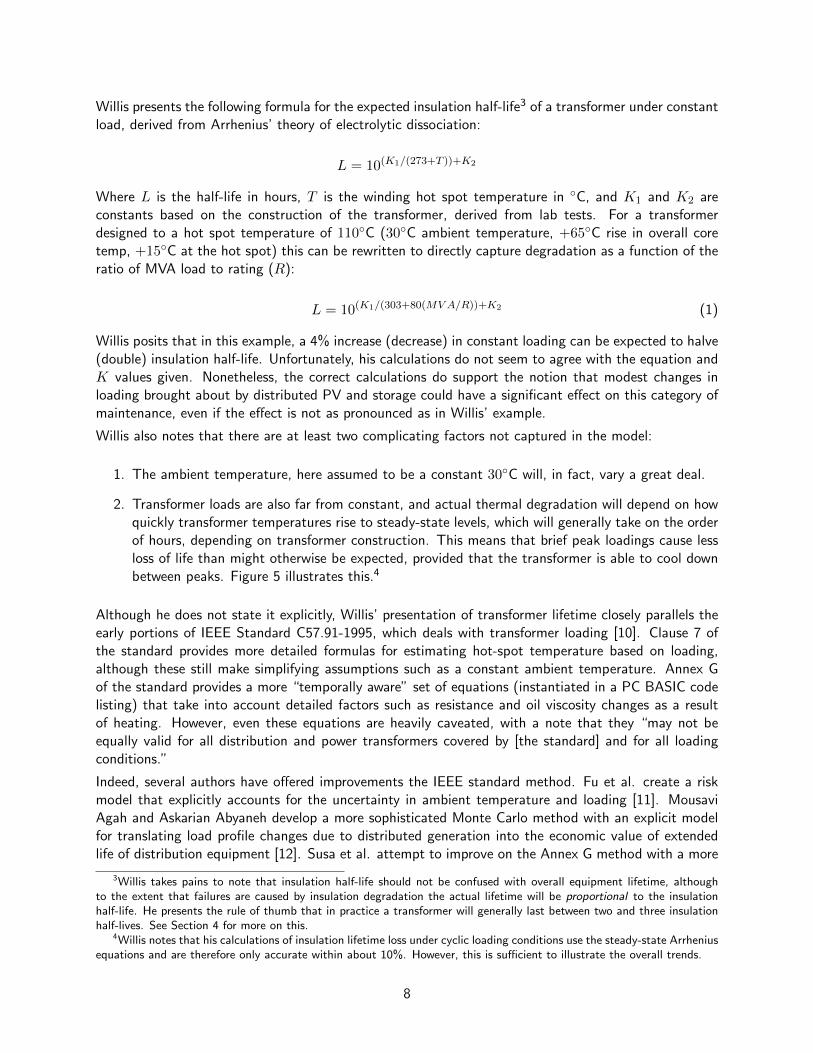
12% of failures are due to physical causes, 61% to fault duty, and 27% to insulation (see Figure 10).Mean life with insulation degradation alone would be 72.7 years at 86% loading. Thus, the ideal lifeextension in this case would have been 45%, whereas the modeled life extension is 21%.

Finally, Figure 11 illustrates mean transformer life as a function of loading ratio in the 100% case,90% case and insulation-failure only case.11 This chart illustrates the diminishing returns of reducingtransformer loading when there are other significant causes of transformer failure. Whereas the Arrheniusequations predict accelerating gains in lifetime as loading is reduced, in this model lifetime hits anasymptotic maximum around 23 years in the 100% base case and 54 years in the 90% base case, asother causes of failure (fault current in particular) come to dominate.

5 Conclusion

In this report, we have outlined a research plan for assessing the economic impact of distributed PVand storage on the distribution system. We have reviewed the likely relationships between loadingchanges brought about by these technologies and the need for distribution capacity and maintenanceexpenditures. In addition, we have presented a probabilistic transformer lifetime model that goes beyondthe existing scholarship by incorporating non-insulation-related failures that are observed by practitionersin the field but have so far been ignored in the peer-reviewed literature. The degree of parameteruncertainty in the model renders it less than ideal for system planning at this stage, but it demonstratespotential to make more realistic lifetime estimates if all causes of failure are taken into account. The keytakeaway from this effort is that system maintenance benefits due to reduced loading are unlikely to beas large in practice as the theoretical literature would suggest when a significant proportion of failures are

11The slight “overshoot” where lifetime is predicted to be higher in the 90% case than the “insulation alone” case athigh loadings is due to the previously-mentioned error introduced by the use of the instantaneous hazard rate in a discretemodel. In this chart the “insulation alone” case was calculated directly from the Arrhenius equation, so it does not includethe small discretization error.

16

Figure 10: 90% base case with 86% loading

Figure 11: Mean transformer lifetime as a function of loading ratio

17

due to causes unrelated to insulation decay. The true magnitude of this benefit “discounting” remainsa topic for further study.

5.1 Next Steps

To conclude, we outline the steps required to bring this project to a successful conclusion.

1. Complete GridLAB-D models.

(a) Populate GridLAB-D taxonomy feeders with PV units whose power production correspondsto data obtained from Solar City.

(b) Obtain and integrate meteorological data corresponding to Solar City generation profiles.This is important because GridLAB-D simulated loads (e.g. HVAC) are weather-dependent,and by default GridLAB-D weather is taken from a “typical meteorological year”. However,the Solar City production data is not necessarily from a typical year. To obtain accurateestimates of the effect of PV on peak loading, the weather that affects the simulated loadsneeds to be the same as the weather that caused the real-life generation.

(c) Design and implement a model of household electricity storage in GridLAB-D.

2. Improve cost models using information from PG&E, manufactures, and other subject matterexperts.

(a) Obtain representative LMPs for use in calculating the economic effects of changes in distri-bution line losses.

(b) Estimate marginal cost of distribution capacity in California based on PG&E work papersand other sources.

(c) Fill in gaps in equipment unit cost data (e.g. cost to replace, rather than repair, a pole-toptransformer).

(d) Attempt to obtain data that would enable refinement of the transformer lifetime modelpresented in Section 4. In particular, data on the age distribution of retired transformersand/or reasons for retirement would be helpful.

3. Integrate GridLAB-D and cost models as shown in Figure 1. That is, run GridLAB-D modelswith varying degrees of PV and storage penetration to obtain metrics of electrical and physicalperformance, then use the economic models to translate these metrics into dollar figures.

4. Simulate additional technologies and scenarios, time and resources permitting. In particular, theuse of four-quadrant “smart” inverters shows promise for alleviating PV-related strain on thedistribution system.

We look forward to working through these remaining steps and providing our final assessment of theimpact of distributed generation and storage on the distribution system.

18

Part II

Integrating Storage Into Emerging CAISOProducts

1 Background and setup

Since its passing, PURPA has mandated that renewables be payed for all power they produce at theavoided cost of traditional generation [17, 18]. With increasing variability from renewable penetration,this will become an untenable arrangement both physically and economically. [add more justification,demonstrating the need for new markets]

Independent System Operators (ISOs) have begun to address some of these issues. Since high pene-trations of wind and solar will require additional power systems services including load following andregulation capacity and ramping [19], ISOs have begun to propose new frameworks to encourage ‘non-generator resources’ (NGRs) [20] such as energy storage devices and demand response (DR) to par-ticipate in energy markets to provide these services. NGRs are widely considered a promising solutionto renewable variability [21, 22, 23]. These new frameworks address the fact that NGRs have differentcapabilities than the traditional power plants that usually provide these services. Specifically, NGR havesmall-to-no ramp constraints but they do have strict energy constraints12 – the total amount of energyprovided/consumed must be “zero mean” over time. To reward NGRs and other fast-ramping resourcesthat can provide 5-minute ramps, the CAISO has also proposed the ‘flexible ramping product’ [24].Moreover, to deal with NGR energy constraints, the California ISO (CAISO) has proposed regulationenergy management (REM), a functionality which would allow the ISO to manage the state of chargeof NGRs so that they can more effectively participate in existing regulation markets [25]. Resources par-ticipating in REM would offer their 15-minute capacity and the CAISO would use the 5-minute marketto ensure that the NGR resources do not saturate.

Traditional spinning reserve markets are run as capacity auctions [26, 27], in which energy capacity isset aside for a premium or capacity payment in a day-ahead market, and then purchased at the real-timemarket price as needed. Similar arrangements are currently being considered for NGRs participating inregulation markets with REM [25]. Characteristics of spinning reserves and regulation make capacitypayments an appropriate format; specifically, generator opportunity costs [28, 29] and the schedulingrequired to comply with unit commitment constraints [30] demand day-ahead planning. Moreover,generator reserves provided at one time are more or less independent from those subsequently neededbecause fuel is generally available in sufficient quantity. On the other hand, unit commitment constraintsare not a factor in NGR markets by design, opportunity costs for firms are substantially lower, and storagecapacity depends on prior decisions. As such, it is worth considering alternative market formats.

In this work, we analyze several new market formats exclusively for NGR resources. Since NGR physicaltransactions are zero-mean, the effect of NGRs is variance reduction, as opposed to traditional resourceswhich both reduce variance and offset average peak demand for generation. We consider two formatsfor NGR markets: (1) day-ahead capacity payments as used for conventional reserves, and (2) nearreal-time markets, in which imbalance fees–payments for providing or consuming energy–are paid toNGRs at time of use, and less or no capacity is procured in the day ahead market. While not traditional,imbalance fees are often assumed in designing competitive wind bidding strategies [31, 32, 33], and areimplemented in some markets, including NordPool [34] and Spain [35]. Our rationale for applying this

12We consider DR resources that may be shifted in time, but not permanently shed.

19

format is two-fold.

• A substantial fraction of storage capacity can be expected to be available despite not having beenprocured ahead of time, because energy storage always has capacity; it may however be positiveor negative.

• Procuring storage capacity in a day-ahead market is stochastic and dynamic because the capacityutilized in one period is random and directly determines that available in the next. This couplingis a major contrast with generator reserve utilization.

New market formats should allow NGRs to reveal their true opportunities and costs to other players inthe power system, and therefore fitting within the definition of hierarchical transactional control [36].

We analyze each format using game theory, which has seen extensive application in analyzing con-ventional power markets. Generator competition is often modeled using supply function equilibrium[37, 38, 39, 40], because bids submitted by generators are often actual supply functions, which reflectnonlinear fuel curves and other generation costs. For NGRs, however, the cost/value of energy is moreor less linear with quantity due to negligible marginal costs. In this extreme case, a supply function isjust a step function; while viable, this may provide flexibility superfluous to storage technologies [thissentence still not clear to me – i get why the supply function is a step function, not sure of the rest].Cournot competition has also been used to model generation competition [41, 42, 43]; however, giventhe uncertain nature of the amount received by each NGR firm, quantity bids are somewhat unrealisticfrom an implementation point of view.

In lieu of these considerations, we model NGR markets with Bertrand-Edgeworth competition [44, 45,46], in which energy storage is patronized up to capacity on the basis of price. Bertrand-Edgeworthcompetition has been widely applied to scenarios in which firms first compete on capacity and thenprice, beginning with [47] in which such scenarios were shown to produce Cournot outcomes. Sincethen, however, limited attention has been devoted to uncertainty, cf. [48, 49]. In this work, we obtainnew results for the case that the object of competition is random. From another perspective, thisscenario is a linear bid, divisible good auction [50, 51]; a similar model was applied to electricity marketdesign in [52]. We build primarily on the work of [53], which is also concerned with capacity followedby price competition.

2 Results

We ultimately obtain a comparison between market formats and market design guidelines. Specificanalysis and results include

• New theoretical characterizations of Bertrand-Edgeworth competition.

• Predictive tools for characterizing potential designs for markets with energy storage.

• Theoretical evidence for the viability and potential superiority of allowing storage to make marketparticipation decision closer to real-time, rather than exclusively making day-ahead commitments.

In particular, we compare market formats described by Tables 1 and 2; to summarize, the former makesstorage procurement decisions in the day ahead market (DAM), and the latter allows storage to commitin a real time market (RTM).

20

Stage Time Competition Description

1 DAM Capacity* The system operator requests capacity C ≤∆ and purchases ∆−C generator reserves.Each firm i specifies a maximum capacitySi ≤ Si.

2 DAM Price Each firm i offers a capacity premium, pi,and the market operator allocates C price-wise among the Si.

3 RTM - All energy is transacted at market price thenext day.

Table 1: Market format M1

Stage Time Competition Description

1 DAM - The system operator purchases ∆− T gen-erator reserves..

2 RTM Capacity Each firm i specifies a maximum capacity,Si ≤ Si.

3 RTM Price Each firm i offers an energy imbalance feepi, and the market operator allocates a ran-dom amount of energy D price-wise amongthe Si.

4 RTM - Energy from storage i is purchased at pi plusthe market price, and spill over is purchasedfrom generator reserves at market price.

Table 2: Market format M2

2.1 Example calculation

Suppose two independent energy storage firms competitively choose energy capacities and prices, andthat in a given time period a random amount of energy is allocated amongst them price-wise in a reservemarket. Denote the cumulative distribution function of the total amount of energy to be absorbed byreserves by F , and assume that it is preferable that storage handle as much of the imbalance as it iswilling and able. Also suppose that R is the maximum the system operator will pay storage, and γS isthe amount storage can make elsewhere, i.e. the opportunity cost incurred for committing capacity Sto the market. Then, in a competitive environment, it can be expected that a combined capacity of

S = F−1(1− γ/R)

will be committed by the firms within the balancing market M2. Now suppose that a total of Γ generatorreserves would have been scheduled without storage. Now, under market format M2, it is known thatΓ − S generator reserves will be scheduled in the day ahead, because storage will make S available inreal time.

The above analysis is an example of a broader framework we are developing for analyzing the competitivebehavior of storage in markets. Ultimately, we will obtain theoretical tools for comparing market formats,and predicting their associated economic outcomes.

21

References

[1] Integration of renewable resources: Operational requirements and generation fleet capability at20% RPS. Technical report, California Independent System Operator, August 2010.

[2] D.P. Chassin, K. Schneider, and C. Gerkensmeyer. GridLAB-D: an open-source power systemsmodeling and simulation environment. In Transmission and Distribution Conference and Exposition,2008. IEEE/PES, pages 1–5, 2008.

[3] K. Schneider, Y. Chen, D. Chassin, R. Pratt, D. Engel, and S. Thompson. Modern grid initiative:Distribution taxonomy final report. Technical report, Pacific Northwest National Lab, Richland,WA, November 2008.

[4] Michael A. Cohen. GridLAB-D taxonomy feeder graphs. http://rollingturtle.com/

gridlabd/taxonomy_graphs/, 2012 February.

[5] Itron, Inc. and Kema, Inc. CPUC california solar initiative 2009 impact evaluation final report.Technical report, June 2010.

[6] Konstantin Turitsyn, Petr Sulc, Scott Backhaus, and Michael Chertkov. Options for control ofreactive power by distributed photovoltaic generators. Proceedings of the IEEE, 99:1063–1073,June 2011.

[7] Thomas E. Hoff, Howard J. Wenger, and Brian K. Farmer. Distributed generation: An alternativeto electric utility investments in system capacity. Energy policy, 24(2):137–147, 1996.

[8] John Carruthers. Personal communication, December 2011.

[9] H. Lee Willis. Equipment ratings, loading, lifetime, and failure. In Power Distribution PlanningReference Book, Second Edition, Power Engineering, chapter 7. CRC Press, March 2004.

[10] IEEE guide for loading Mineral-Oil immersed transformer. IEEE Standard C57.91-1995, 1995.

[11] W. Fu, J.D. McCalley, and V. Vittal. Risk assessment for transformer loading. Power Systems,IEEE Transactions on, 16(3):346–353, 2001.

[12] S. M. Mousavi Agah and H. Askarian Abyaneh. Quantification of the distribution transformer lifeextension value of distributed generation. IEEE Transactions on Power Delivery, 26:1820–1828,July 2011.

[13] D. Susa, M. Lehtonen, and H. Nordman. Dynamic thermal modelling of power transformers. IEEETransactions on Power Delivery, 20:197–204, January 2005.

[14] Pacific Gas & Electric. PG&E 2011 general rate case prepared testimony exhibit 3, gas and electricdistribution, December 2009.

[15] Pankaj K Sen and Steven L Larson. Fundamental concepts of regulating distribution system volt-ages. In Rural Electric Power Conference, 1994. Papers Presented at the 38th Annual Conference,pages C1–1–C1–10, 1994.

[16] D. Kirshner. Implementation of conservation voltage reduction at Commonwealth Edison. PowerSystems, IEEE Transactions on, 5(4):1178–1182, 1990.

22

[17] Paul L. Joskow and Richard Schmalensee. Markets for Power: An Analysis of Electrical UtilityDeregulation. MIT Press Books. The MIT Press, March 1988.

[18] Paul L. Joskow. Restructuring, competition and regulatory reform in the u.s. electricity sector. TheJournal of Economic Perspectives, 11(3):119–138, 1997.

[19] Y. V Makarov, C. Loutan, J. Ma, and P. De Mello. Operational impacts of wind generation oncalifornia power systems. IEEE Transactions on Power Systems, 24(2):1039–1050, 2009.

[20] CAISO. Revised draft final proposal for participation of Non-Generator resources in California ISOancillary services markets. Technical report, CAISO, Mar 2010.

[21] J.P. Barton and D.G. Infield. Energy storage and its use with intermittent renewable energy. EnergyConversion, IEEE Transactions on, 19(2):441 – 448, Jun. 2004.

[22] J.M. Carrasco, L.G. Franquelo, J.T. Bialasiewicz, E. Galvan, R.C.P. Guisado, Ma.A.M. Prats, J.I.Leon, and N. Moreno-Alfonso. Power-electronic systems for the grid integration of renewable energysources: A survey. Industrial Electronics, IEEE Transactions on, 53(4):1002 –1016, Jun. 2006.

[23] D.S. Callaway and I. A. Hiskens. Achieving controllability of electric loads. Proceedings of theIEEE, 99(1):184–199, January 2011.

[24] CAISO. Flexible ramping product and cost allocation, Dec 2011.

[25] California ISO. Regulation energy management draft final proposal, January 2011.

[26] H. Singh and A. Papalexopoulos. Competitive procurement of ancillary services by an independentsystem operator. Power Systems, IEEE Transactions on, 14(2):498 –504, May 1999.

[27] E.H. Allen and M.D. Ilic. Reserve markets for power systems reliability. Power Systems, IEEETransactions on, 15(1):228 –233, Feb. 2000.

[28] M. Shahidehpour, H. Yamin, and Z. Li. Market Operations in Electric Power Systems (Forecasting,Scheduling, and Risk Management). Wiley-IEEE Press, 2002.

[29] Tongxin Zheng and E. Litvinov. Ex post pricing in the co-optimized energy and reserve market.Power Systems, IEEE Transactions on, 21(4):1528 –1538, Nov. 2006.

[30] A. J. Wood and B. F. Wollenberg. Power generation, operation, and control. Knovel, secondedition, 1996.

[31] John Bj∅rnar Bremnes. Probabilistic wind power forecasts using local quantile regression. WindEnergy, 7(1):47–54, 2004.

[32] P. Pinson, C. Chevallier, and G.N. Kariniotakis. Trading wind generation from short-term proba-bilistic forecasts of wind power. Power Systems, IEEE Transactions on, 22(3):1148 –1156, Aug.2007.

[33] E. Bitar, A. Giani, R. Rajagopal, D. Varagnolo, P. Khargonekar, K. Poolla, and P. Varaiya. Optimalcontracts for wind power producers in electricity markets. In Decision and Control (CDC), 201049th IEEE Conference on, pages 1919 –1926, Dec. 2010.

[34] Klaus Skytte. The regulating power market on the Nordic power exchange Nord pool: an econo-metric analysis. Energy Economics, 21(4):295 – 308, 1999.

23

[35] Julio Usaola, Oswaldo Ravelo, Gerardo Gonzalez, Fernando Soto, M. Carmen Davila, and BelenDıaz-Guerra. Benefits for wind energy in electricity markets from using short term wind powerprediction tools; a simulation study. Wind Engineering, 28(1):119–127, Jan. 2004.

[36] D. Hammerstrom, T. Oliver, R. Melton, and R. Ambrosio. Standardization of a hierarchical trans-active control system. Proceedings of the Grid Interop, 9, 2007.

[37] Paul D. Klemperer and Margaret A. Meyer. Supply function equilibria in oligopoly under uncertainty.Econometrica, 57(6):1243–1277, 1989.

[38] Richard J. Green and David M. Newbery. Competition in the British electricity spot market. Journalof Political Economy, 100(5):pp. 929–953, 1992.

[39] C.J. Day, B.F. Hobbs, and Jong-Shi Pang. Oligopolistic competition in power networks: a con-jectured supply function approach. Power Systems, IEEE Transactions on, 17(3):597 – 607, Aug.2002.

[40] Ross Baldick, Ryan Grant, and Edward Kahn. Theory and application of linear supply functionequilibrium in electricity markets. Journal of Regulatory Economics, 25:143–167, 2004.

[41] B.F. Hobbs, C.B. Metzler, and J.-S. Pang. Strategic gaming analysis for electric power systems:an MPEC approach. Power Systems, IEEE Transactions on, 15(2):638 –645, May 2000.

[42] B.E. Hobbs. Linear complementarity models of Nash-Cournot competition in bilateral and POOLCOpower markets. Power Systems, IEEE Transactions on, 16(2):194 –202, May 2001.

[43] Judith B. Cardell, Carrie Cullen Hitt, and William W. Hogan. Market power and strategic interactionin electricity networks. Resource and Energy Economics, 19(1-2):109 – 137, 1997.

[44] J. Bertrand. Theorie mathematique de la richesse sociale. Journaldes Savants, pages 499–508,1883.

[45] F.Y. Edgeworth. The pure theory of monopoly. In Papers relating to political economy, volume 1,pages 111–142. Macmillan and Co., Ltd., 1925.

[46] X. Vives. Oligopoly pricing: old ideas and new tools. MIT Press, 2001.

[47] David M. Kreps and Jose A. Scheinkman. Quantity precommitment and bertrand competition yieldcournot outcomes. The Bell Journal of Economics, 14(2):326–337, 1983.

[48] Marıa Angeles de Frutos and Natalia Fabra. Endogenous capacities and price competition: The roleof demand uncertainty. International Journal of Industrial Organization, 29(4):399 – 411, 2011.

[49] Stanley S. Reynolds and Bart J. Wilson. Bertrand-Edgeworth competition, demand uncertainty,and asymmetric outcomes. Journal of Economic Theory, 92(1):122 – 141, 2000.

[50] Robert Wilson. Auctions of shares. The Quarterly Journal of Economics, 93(4):pp. 675–689, 1979.

[51] V. Krishna. Auction Theory. Academic Press/Elsevier, 2009.

[52] Natalia Fabra, Nils-Henrik von der Fehr, and David Harbord. Designing electricity auctions. TheRAND Journal of Economics, 37(1):23–46, 2006.

[53] Daron Acemoglu, Kostas Bimpikis, and Asuman Ozdaglar. Price and capacity competition. Gamesand Economic Behavior, 66(1):1 – 26, 2009.

24