Embed Size (px)
Citation preview

INTERFERENCE MITIGATION IN RADIO ALTIMETER
A Thesis
by
JYOTHSNA KURRA
Submitted to the Office of Graduate and Professional Studies of Texas A&M University
in partial fulfillment of the requirements for the degree of
MASTER OF SCIENCE
Chair of Committee, Scott L. Miller Committee Members, Krishna Narayanan Srinivas Shakkottai John Valasek Head of Department, Miroslav M. Begovic
December 2018
Major Subject: Electrical Engineering
Copyright 2018 Jyothsna Kurra

ii
ABSTRACT
Ever since its advent in the late 19th century, wireless technology has evolved substantially.
Towards the end of 20th century, wireless system was being considered as a replacement for wired
connections between digital avionic systems in an aircraft. Although it seemed to be a possible
breakthrough in aviation, it came with its own set of challenges which included interference
avoidance with aircraft electronics, dedicated reserved frequency band and many more. Hence, the
existing wireless solutions could not be used directly and there is a need to develop specialized
solutions.
The primary objective of this research is to devise a technique to manage the interference,
arising due to the Wireless Avionics Intra-Communication (WAIC) System, in the radio altimeter
present in an aircraft. The altimeter along with the in-flight environment has been simulated in
MATLAB. Its performance has been evaluated for the scenario when the interference due to WAIC
system is introduced. Also, various techniques which utilize vacant bandwidth of the altimeter to
aid the avionics intra-communication, thus managing the interference for the altimeter, have been
analyzed.

iii
DEDICATION
To my parents

iv
ACKNOWLEDGEMENTS
I would like to express my sincere gratitude to my advisor, Dr. Scott L. Miller, for steering
my first endeavor in academic research through his guidance, patience and understanding. I find
myself extremely lucky to have an advisor, who responded to all my queries and requests so
promptly.
I would like to thank Dr. Krishna Narayanan and Dr. John Valasek for serving on my thesis
committee. I am deeply obligated to Dr. Srinivas Shakkottai for agreeing to be a part of my thesis
committee in the absence of Dr. Gregory Huff.
I am grateful to Vamsi Krishna Amalladinne for discussing some fine technical aspects,
which helped clear a few roadblocks in my research. I thank Deepika Ravipati for offering
invaluable resources to pursue this research.
I wish to thank the department of Electronics and Computer Engineering at TAMU for
providing the necessary resources to fulfill my academic ambition.
I am obliged to all my friends for helping me keep my life in context. I would like to thank
my family for their undetering support, encouragement and faith in me.

v
CONTRIBUTORS AND FUNDING SOURCES
This work was supported by a thesis committee consisting of Professor Scott L. Miller,
Professor Krishna Narayanan and Professor Srinivas Shakkottai of the Department of Electronics
and Computer Engineering and Professor John Valasek of the Department of Aerospace
Engineering.
All work for the dissertation was completed independently by the student.

vi
NOMENCLATURE
WAIC Wireless Avionics Intra-Communication
AVSI Aerospace Vehicle Systems Institute
ICAO International Civil Aviation Organization
ITU International Telecommunication Union
EMI Electro-Magnetic Interference
WRC World Radio Communication
ARNS Aeronautical Radio Navigation Service
RADALT Radio Altimeters
AGL Above Ground Level
GPWS Ground Proximity Warning Systems
EM Electro-Magnetic
FMCW Frequency Modulated Continuous Wave
LFM-CW Linear Frequency Modulated Continuous Wave
AWGN Additive White Gaussian Noise
SNR Signal to Noise Ratio
SINR Signal to Interference plus Noise Ratio
MAC Medium Access Control
IM Interference Management
PSD Power Spectral Density

vii
TABLE OF CONTENTS
Page
ABSTRACT ............................................................................................................................... ii
DEDICATION........................................................................................................................... iii
ACKNOWLEDGEMENTS ....................................................................................................... iv
CONTRIBUTORS AND FUNDING SOURCES ........................................................................ v
NOMENCLATURE .................................................................................................................. vi
TABLE OF CONTENTS .......................................................................................................... vii
LIST OF FIGURES ................................................................................................................... ix
LIST OF TABLES ...................................................................................................................... x
CHAPTER I INTRODUCTION AND LITERATURE REVIEW ............................................... 1
1.1 Wireless Avionics Intra-Communication (WAIC) System .............................................. 2 1.1.1 Advantages of WAIC System .............................................................................. 4 1.1.2 Challenges faced by WAIC system ...................................................................... 6
1.1.2.1 Spectrum Allocation for WAIC system ................................................. 7 1.2 Need for Interference Management ................................................................................ 7 1.3 Radio Altimeter ............................................................................................................. 8
1.3.1 Operating Principle of Radio Altimeter ................................................................ 9 1.3.2 Frequency Modulated Continuous Wave (FMCW) Altimeter ............................. 11
CHAPTER II SIMULATION OF FMCW ALTIMETER ......................................................... 15
2.1 Linear Frequency Modulated (Chirp) Signal ................................................................ 15 2.2 In-Flight Environment.................................................................................................. 18 2.3 Altitude Calculation ..................................................................................................... 19 2.4 Test Setup .................................................................................................................... 23

viii
CHAPTER III ANALYSIS OF INTERFERENCE MANAGEMENT TECHNIQUES ............. 26
3.1 Transmit Beamforming Approach ................................................................................ 27 3.2 Spectral Shaping Approach .......................................................................................... 28 3.3 Spread Spectrum Approach .......................................................................................... 30 3.4 Spectrum Sensing-based Approach .............................................................................. 32 3.5 Time-Synchronized IM Technique ............................................................................... 33
CHAPTER IV CONCLUSION ................................................................................................ 37
REFERENCES ......................................................................................................................... 38

ix
LIST OF FIGURES
FIGURE Page
1. Wiring in a typical commercial aircraft …………………………………………… 2
2. Potential WAIC Applications ……………………………………………………… 5
3. Operating Principle of a Radio Altimeter …………………………………………. 10
4. Frequency variation of FMCW altimeter waveform w.r.t time ………………….... 11
5. An Up-Chirp Signal Waveform ………………………………………………….... 16
6. Spectrogram of the up-chirp signal shown in figure 5 …………………………...... 16
7. Correlation Peak at t » 5ms, indicating that t » 5ms ………………………………. 21
8. Analysis of Fine Errors occurring in an altimeter ………………………………......24
9. Performance of altimeter errors in the absence of interference management ……... 25
10. Characterization of Spectral Shaping …………………………………………...…. 29
11. Performance of the altimeter when spectral shaping technique was used.……….... 29
12. Characterization of Spread Spectrum ……………………………………………… 31
13. Performance of altimeter when spread spectrum technique was used .……………. 31
14. Performance of altimeter when time-synchronized IM technique was used ……… 34
15. Performance of Altimeter at SINR = 14 dB for varying Guard Interval ………….. 35
16. Performance of Altimeter for varying Guard Interval on a Logarithmic Scale…..... 36

x
LIST OF TABLES
TABLE Page
1. Technical Characteristics of typical Analog FMCW Altimeters ………………….. 13
2. Technical Characteristics of typical Digital FMCW Altimeters ………………….. 14
3. Comparison of different transmitter-end IC techniques ………………………....... 27
4. Number of Outliers observed for different Interference Mitigation Techniques ..... 36

1
CHAPTER I
INTRODUCTION AND LITERATURE REVIEW
Airplanes have been regarded as the one of the most important innovations in the history
of transportation. They revolutionized the war scenario and aided in socio-economic growth in the
post-war era. Over the past few decades, aviation technology has witnessed a rapid development.
Today, aircrafts are capable of transporting goods and people from one part of the world to another
in less than a day. They play critical roles in the events of disasters and medical emergencies.
Hence, ensuring their safety and reliability becomes very important. The proper functioning of an
aircraft is ensured partly by its avionics.
The term avionics is an amalgamation of the words aviation and electronics. It is a
humongous network of electronic systems that perform individual functions on an aircraft. It is
comprised of electronics that support communications, navigation, monitoring displays, flight
control system, flight recording system, collision avoidance system and hundreds of other systems
that are instrumental in the management of the aircraft.
In a modern-day aircraft, all the avionic systems are connected using wires. Although, these
wires are critical to the functioning of the aircraft, they form a very complex system (see figure 1).
A major reason for this complexity is the incorporation of redundant wiring. A wire may fail due
to incorrect installation, wear and tear induced by the environment or manufacturing flaws at any
given point of time. Therefore, in order to avoid a system paralysis due to failure in a
communication wire, redundancy is introduced into the wiring system. Currently, for each wire,
there exist two or three redundant wires. This leads to a huge number of wires to be installed in
the aircraft. A modern twin-aisle aircraft like the Boeing 787 has about 100,000 wires which could

2
extend for 470 kilometers. This is approximately the distance between Los Angeles and San Jose!
These wires weigh nearly 5,700 kilograms, which accounts for almost 3% of the aircraft’s weight
[1]. Such an enormous amount of weight, in turn, affects the fuel efficiency of the aircraft.
Figure 1: Wiring in a typical commercial aircraft (Reprinted from [2])
In order to enhance the efficiency, safety and reliability of the avionics intra-
communication system, the Civil Aviation Industry came up with the idea of a Wireless Avionics
Intra-Communication (WAIC) system.
1.1 Wireless Avionics Intra-Communication (WAIC) System
Towards the end of 20th century, aerospace researchers started to investigate the possibility of
utilizing wireless connectivity to implement cable-less avionics for enhanced efficiency and

3
reliability at reduced cost [3]. It has been estimated that around 30% (1,800 kilograms) of the wires
could be potentially replaced by wireless links [4].
The aim of WAIC system is to provide radiocommunication between two or more stations
on a single aircraft and constitute exclusive closed on-board networks required for the operation
of an aircraft. These stations may be realized using integrated wireless components like wireless
sensors. WAIC systems will not provide air-to-ground, air-to-satellite or air-to-air communications
and will not be used for in-flight entertainment purposes. They will only be used for safety-related
aircraft applications. [5]
The WAIC system layout may vary depending on the type of aircraft. It need not
necessarily be limited to the interior of the aircraft structure. For example, the fuel gauge or the
transmitter for fuel information will be present in the wing of the aircraft and receiver for this
information will be in the cockpit. WAIC systems are currently planned to be installed on a variety
of aircrafts which include regional, business, wide-body, two-deck aircraft and helicopters.
Since the WAIC systems are supposed to be installed on aircrafts, they need to follow
international standards as aircrafts cross international boundaries quite often. Hence, national as
well as international organizations are involved in the project. The WAIC system is currently being
researched by AVSI (Aerospace Vehicle Systems Institute), ICAO (International Civil Aviation
Organization) and ITU (International Telecommunication Union).
In addition to fuel reduction and subsequent environmental benefits, the use of Wireless
Avionics Intra-Communications (WAIC) systems are anticipated to reduce the complexity of
aircraft design. This will in turn improve an aircraft’s performance over its useful lifetime through
more cost-effective flight operations, reduction in maintenance costs and enhancement of aircraft
systems that maintain or increase the level of safety. [6]

4
The prospective advantages of WAIC systems have been discussed in detail below.
1.1.1 Advantages of WAIC System
Wires and cables are gaining increasing importance more than ever in the data-centric architecture
of modern aircraft.
On an average, wiring on a modern aircraft ranges anywhere between 70-300 miles. [7]
They present the aircraft manufacturers and operators with a substantial expense, which is, in turn,
levied on to the end customer. These expenses comprise of wiring harness designs, labor-intensive
harness fabrication as well as maintenance and replacement costs of flying copper and connectors.
Designing and installing a wiring harness consumes a lot of time as it requires explicit
determination of routes for all the connections onboard an aircraft. It is necessary that redundant
connections follow a separate path, in order to isolate the redundant circuits from issues affecting
the main circuit. Being a tedious process, this shoots up the costs associated with wiring harness
design and installation. Clearly, the use of wireless products would save a lot of time, effort and
money for aircraft industry.
Additionally, with the wireless system providing the primary connection and only one
redundant wired path in place, common mode failures could be avoided. Such a dissimilar
redundancy promises higher reliability over the traditional wired architecture in which all the
connections related to a particular system, could possibly fail for the same reason.
Wires also act as undesired transceivers, transmitting and receiving unwanted
electromagnetic energy from the surrounding circuitry. Thus, additional resources need to be
invested to ensure proper shielding from the electromagnetic interference (EMI). It is estimated

5
that around 50% of EMI onboard an aircraft is a result of the wiring system. This encourages the
need to find an alternative to the wired system.
An aircraft is operable for about 30 years on an average. [8] The avionics present onboard
are expected to be functioning throughout the lifetime of the aircraft. However, due to the operating
conditions, wear and tear is induced onto the electronic components, especially the monitoring
sensors and hence, they undergo replacements. Sometimes, components are merely replaced to
introduce updates. Given the complicated layout of the wiring, fault-finding and
repairing/replacing the electronics becomes a very tedious task. On the contrary, the WAIC system
provides considerable flexibility towards the modification of electronics systems and structural
monitoring.
Figure 2: Potential WAIC Applications
As discussed earlier in 1.1, the WAIC system could help reduce the aircraft weight by more
than 25%. This can be utilized to install new avionics, that can help provide better monitoring of

6
the health of the aircraft. For example, sensors could be installed to monitor the temperature of the
components, thus, curbing the attrition induced on the circuit due to heat. Also, additional
functionalities could be implemented using wireless technology, which could not be achieved
using wires. For example, sensors could be installed on moving or rotating parts and information
regarding the rotor parameters could be transmitted to the desired location on the aircraft.
Furthermore, with wireless technology, cabin reconfiguration would become adaptive, i.e.,
reconfiguring the seat layout would become relatively easy and quick.
Thus, the WAIC system ensures enhanced reliability as it rules out the losses induced due
to wires as well as the need for maintenance to resolve issues arising due to wear & tear and aging
of wires, which are unavoidable in the traditional wired architecture.
1.1.2 Challenges faced by WAIC system
Although the WAIC system seemed promising, it was not until recently that it could be realized
due to a number of challenges faced in the past decade.
One of the major problems was the lack of a dedicated frequency band for WAIC system.
Any communication system consists of a transmitting end, a receiving end and a channel. In case
of wireless communication, the channel is characterized by a specific radio frequency or a band of
radio frequencies, usually approved by an international regulatory committee for use.
Since, there are many other on-board wireless radio-communications services, it is
necessary that these services do not interfere with the operation of WAIC system and vice-versa.
Hence, the popular unlicensed frequency bands (2.4GHz and 5 GHz) were rejected for setting up
wireless links in regard to safety-related applications. [9] Moreover, aircrafts often cross
international territorial boundaries. Therefore, it was very important that the WAIC systems was

7
allocated a dedicated frequency band, so as to avoid interference with any radio-communication
service that could possibly function in its proximity.
[10] discusses the design issues of WAIC system ranging from physical layer to application
and security layers. A few other notable challenges introduced by WAIC were,
1. Establishing highly secured communication
2. Avoiding interference with aircraft electronics
3. Enabling anti-jamming property
1.1.2.1 Spectrum Allocation for WAIC system
Several frequency bands were investigated for their compatibility to the WAIC system. [11] [12]
[13] In the World Radio Communication (WRC) Conference 2015, the WAIC system was finally
allotted a spectrum ranging from 4.2 GHz to 4.4 GHz.
However, unlike the requirement, the allocated band of frequencies was not explicit to
WAIC applications. This spectrum was earlier allocated to Aeronautical Radio Navigation Service
(ARNS) and was already being used by the radio altimeters (RADALT) installed on aircrafts.
This presented AVSI and the associated organizations, who were researching on WAIC,
with a new challenge of ‘Interference Management’.
1.2 Need for Interference Management
The WAIC system supports safety-related applications, which provide important statistics
regarding the health of the aircraft and hence, it could not be disrupted for a long period of time.
On the other hand, according to [14], the altimeter is a critical component of safety and thus, it

8
cannot suffer from disruptions, even for short periods of time. Therefore, it becomes necessary
that the signals of the two systems do not interfere with one another in a destructive fashion.
[15] discusses about the different interference mitigation techniques that could enable
reliable operation of WAIC system in the presence of radio altimeters. Also, various researchers
[11] [16] [17] have analyzed the effect of interference on the radio altimeters due to WAIC system.
However, none have suggested solutions towards interference management in altimeters. The goal
of this report is to propose efficient techniques to mitigate the interference experienced by the radio
altimeter due to the WAIC system.
1.3 Radio Altimeter
According to [18], a radio altimeter is a radio navigation equipment, on board an aircraft, used to
determine the height of the aircraft above the Earth's surface or another surface. The very first
radio altimeter was invented by an American engineer Lloyd Espenschied in 1924. It was used by
an aircraft for the very first time as a terrain avoidance system in 1938. [19]
Radar altimeter measures absolute altitude, also referred to as the height Above Ground
Level (AGL). Depending on the type of aircraft, there might be up to 3 radar altimeters installed
on-board. [19] All the three altimeters operate simultaneously and independent of one another.
This is done to increase the accuracy of altitude measurement.
Normally, a radio altimeter can measure altitudes ranging from -20 feet (-6 meters) up to
19,685 feet (6000 meters) with an accuracy of 3 feet (0.9 meters).
Radio altimeters are a crucial component of Ground Proximity Warning Systems (GPWS).
Commercial aircrafts mainly use altimeter during approach, landing and low-level or low-visibility
flight conditions. It provides the necessary altitude information in regard to landing decision

9
height. The safe altitude to land can be set beforehand. The altimeter sends a warning to the pilot
when the aircraft reaches the predetermined altitude. Normally, landing is aborted if the pilot
receives a warning and runway is not visible. Otherwise, the flare maneuver is initiated for a safe
landing.
The ITU-R [18] considers the radio altimeter an essential component of aeronautical
safety-of-life systems. For this reason, operation of radio altimeter should not be disrupted at any
cost. So, it is crucial to protect it from interferences, including that arising from the WAIC signals.
Before proceeding to the different interference mitigation techniques, it is important to understand
the operating principle of a radar altimeter.
1.3.1 Operating Principle of Radio Altimeter
The underlying principle of a radio altimeter is radar. Radar is a system that uses high-frequency
electromagnetic (EM) waves to determine distance, direction and velocity of other objects. The
frequency of the EM waves used in an altimeter often belong to the radio or microwave domain of
EM spectrum. Hence, radar altimeters are also known as ‘Radio Altimeter’.
A typical radio altimeter consists of a transmitter and a receiver. The transmitter is
responsible for producing radio waves and transmitting them down to ground. These waves
propagate in the atmosphere, hit the terrain and get reflected back to the receiver. The receiver
then processes the received waves to compute the altitude. Typically, an altimeter measures the
time taken for the transmitted radio wave to reach the receiving antenna and calculates the altitude
(ℎ) using speed of light as shown in the below equation.
ℎ =𝑐x𝑇2 (1)
where, 𝑇 is the time taken for the transmitted wave to reach the receiving antenna

10
and 𝑐 is the speed of light = 3 x 10⁸ m/s
Figure 3: Operating Principle of a Radio Altimeter (Reprinted from [20])
Since, the radio waves propagate at the speed of light, the propagation time is usually very
small, in the order of microseconds. A single antenna cannot switch between transmission and
reception in a such a short period of time. Hence, two different antennas are installed in each
altimeter for the purpose of transmission and reception of radio waves. To ensure proper operation
of the altimeter, the receiving antenna should only pick up the reflected radio wave and avoid all
other signals, including the transmitted wave. Hence, in order to avoid unwanted cross talk
between the transmitted and receiving antennas, they are widely separated.

11
1.3.2 Frequency Modulated Continuous Wave (FMCW) Altimeter
Based on the modulation of the transmitted EM waves, radar altimeters are broadly classified into
two categories,
• Pulsed Altimeter
• Linear Frequency Modulated Continuous Wave (LFM-CW) Altimeter
The LFM-CW altimeter, simply known as FMCW altimeter is identified to achieve higher
accuracy over pulsed altimeter. Hence, FMCW altimeters are the industry standard. Today, all
commercial aircrafts utilize FMCW altimeters. [21]
FMCW altimeters utilize large bandwidths to achieve the necessary accuracy levels. If the
frequency bandwidth of an altimeter is reduced, the accuracy gets affected proportionately. [14]
FMCW altimeters use doppler effect in determining the altitude of the aircraft. The
transmitter generates a linear frequency modulated signal, whose frequency varies continuously in
Figure 4: Frequency variation of FMCW altimeter waveform w.r.t time

12
the range of 4.2 – 4.4 GHz. As mentioned earlier in 1.3.1, the transmitted signal takes a short while
to reach the receiving antenna. By the time the reflected EM wave reaches the receiver, the
frequency of the signal at the transmitter is changed. FMCW altimeter works on the principle that
the propagation time for the EM wave is directly proportional to the difference between the
operating frequencies of transmitting and receiving antennas. [22] Thus, at any given instant of
time, the altitude of the aircraft is directly proportional to the difference between the transmitter
and receiver frequencies. From equation (1), the altitude h is given as,
ℎ = 𝑐x𝑇2
(𝑜𝑟)ℎ =𝑐x∆𝑡2
⟹ ℎ =𝑐x∆𝑓
2 1𝑑𝑓𝑑𝑡3(2)
where, 4546
represents the rate at which the signal frequency sweeps across the available bandwidth.
(Typically, 4546= 200𝐻𝑧)
Here, it has been assumed that the signal frequency is not affected by propagation environment
and it remains unchanged till it reaches the receiver.
Technical characteristics of typical analog and digital FMCW radio altimeters have been
provided in Table 1 and Table 2.

13
Table 1: Technical Characteristics of typical Analog FMCW Altimeters (Reprinted from [14])
ALTIMETER A1 ALTIMETER A2 ALTIMETER A3
Nominal Centre
Frequency (in MHz) 4300 4300 4300
Transmitted Peak
Power (in W) 0.6 1 0.1 to 0.25
Chirp Bandwidth
excluding temperature
drift (in MHz)
104 132.8 133
Altitude Measurement
Range (meters/feet)
-4.6 to +2500 m
(or) -15 to +8200 ft
-6 to +2438 m
(or) -20 to +8000 ft
-6 to +6000 m (or)
-20 to +19685 ft
Operational Altitude (in
km) 12 12 20
Maximum Frequency
Drift over Operational
Temperature Range (in
MHz)
±15 ±15 ±20
Centre frequency offset
between individual
radio altimeter systems
(In MHz)
5 5 0
Waveform repetition
frequency (Hz) 49 to 51 150 12 to 1623

14
Table 2: Technical Characteristics of typical Digital FMCW Altimeters (Reprinted from [14])
ALTIMETER D1 ALTIMETER D2 ALTIMETER D3
Nominal Centre
Frequency (in MHz) 4300 4300 4300
Transmitted Peak
Power (in W) 0.4 0.1 0.1 to 1
Chirp Bandwidth
excluding temperature
drift (in MHz)
150 176.8 133
Altitude Measurement
Range (meters/feet)
-6 to +1676 m
(or) -20 to +5500 ft
-6 to +1737 m
(or) -20 to +5700 ft
-6 to +6000 m (or)
-20 to +19685 ft
Operational Altitude (in
km) 12 12 20
Maximum Frequency
Drift over Operational
Temperature Range (in
MHz)
±0.22 ±0.129 ±0.22
Average number of
systems installed per
aircraft
2 or 3 2 or 3 1 or 2
Waveform repetition
frequency (Hz) 143 1000 100 to 4700

15
CHAPTER II
SIMULATION OF FMCW ALTIMETER
In order to analyze the proposed interference mitigation schemes, a test bed to emulate the FMCW
altimeter under normal operating conditions was set up. This involved simulating,
• Altimeter Transmitter
• Channel (in-flight environment)
• Altimeter Receiver
Details pertaining to the simulation development have been discussed below.
2.1 Linear Frequency Modulated (Chirp) Signal
As mentioned in 1.3.2, the FMCW transmitter generates a linear frequency modulated signal,
which is often also referred to as “Linear Chirp” or “Linear Sweep” signal in the literature. It owes
its funny name due to its profound similarity to the chirping sound made by birds. [23]
The frequency of a chirp signal changes (either increases or decreases) with time. If the
frequency of the signal increases with time, it is known as up-chirp signal (see figure 5). Similarly,
if the frequency decreases with time, it is called down-chirp signal.
Let 𝑠(𝑡)be any sinusoidal signal with phase 𝜃(𝑡) as defined below.
𝑠(𝑡) = sin?𝜃(𝑡)@(3)
As mentioned above, 𝑠(𝑡) is a chirp signal if its frequency varies with time. The instantaneous
frequency of a chirp signal is the rate of change of the signal phase as shown below.
𝑓(𝑡) = 12𝜋
𝑑𝜃(𝑡)𝑑𝑡 (4)

16
Figure 5: An Up-Chirp Signal Waveform
Figure 6: Spectrogram of the up-chirp signal shown in figure 5
0 0.1 0.2 0.3 0.4 0.5 0.6 0.7 0.8 0.9 1time (ms) 10-3
-1
-0.8
-0.6
-0.4
-0.2
0
0.2
0.4
0.6
0.8
1
Ampl
itude
Chirp Waveform
Spectrogram of Chirp
100 200 300 400 500 600 700 800time (ms)
0
50
100
150
200
250
300
350
400
450
frequ
ency
(MH
z)
-110
-100
-90
-80
-70
-60
-50
-40
Pow
er/fr
eque
ncy
(dB/
Hz)
17
For a linear chirp signal, the instantaneous frequency varies linearly with time and hence, could be
formulated as,
𝑓(𝑡) = 𝑓D + 𝑘𝑡(5)
where, 𝑓D is the initial frequency (at time, 𝑡 = 0)
and 𝑘 is a scalar which represents the rate of change in frequency, also known as sweep rate or
chirpyness and is given by,
𝑘 = 𝑑𝑓𝑑𝑡 =
𝑓H −𝑓D𝑇 (6)
𝑓H is the final frequency (at time, 𝑡 = 𝑇)
From (4), the instantaneous phase could be written as,
𝜃(𝑡) = 𝜃D + 2𝜋K 𝑓(𝜏)𝑑𝜏6
D(7)
𝜃(𝑡) = 𝜃D + 2𝜋K (𝑓D + 𝑘𝜏)𝑑𝜏6
D(8)
⇒ 𝜃(𝑡) = 𝜃D + 2𝜋 1𝑓D𝑡 +𝑘2 𝑡
P3(9)
where, 𝜃D is the initial phase (at time, 𝑡 = 0)
Thus, the linear chirp signal could be written as,
𝑥(𝑡) = sinS𝜃D + 2𝜋 1𝑓D𝑡 +𝑘2 𝑡
P3T(10)
To keep things simple during simulation, a complex baseband equivalent of the band pass
signal was considered. Hence, the initial phase and frequency were assumed to be 0 radians and 0
Hz respectively. 𝑘 was chosen based on the value of waveform repetition frequency for the desired
altimeter from Table 1 and Table 2.

18
Once a chirp signal was generated according to the specifications of the desired FMCW
altimeter, the value of the altitude to be emulated was decided and the corresponding propagation
time was computed using equation (1). The generated chirp signal was delayed by the calculated
propagation time to reproduce the EM signal at the receiving antenna.
2.2 In-Flight Environment
The receiving antenna of an altimeter is surrounded by numerous electronic components, which
contribute to thermal noise, shot noise, flicker noise, burst noise and transit time noise. The amount
of noise produced varies greatly depending on the operating temperature and type of device. Most
of these noises, especially thermal noise is unavoidable, given the altimeter operating conditions.
Thermal noise, also known as Johnson noise or Nyquist noise or Johnson-Nyquist noise, is
in fact, one of the major sources of noise in electronic circuits. It is generated due to thermal
agitation of charge carriers, usually electrons, within an electrical conductor at equilibrium. It
occurs irrespective of the applied voltage because agitation in charge carriers is caused due to
temperature. For high temperatures, the charge carriers experience greater levels of agitation and
hence, the amount of thermal noise increases.
Thermal noise is quite random in nature. It has been found that the amplitude follows a
Gaussian probability density function. [24] Furthermore, it is a white noise i.e., the power spectral
density is almost constant throughout the frequency spectrum. Hence, it is frequently modelled as
additive white gaussian noise (AWGN).
For purpose of simulation, AWGN corresponding to a SNR of 17 dB was generated. It
could be seen from figure 8 that the altimeter could function correctly when its signal to noise ratio
(SNR) was greater than or equal to 17 dB. Hence, in order to analyze the effects of interference on

19
the altimeter, the least possible SNR for which the altimeter could function properly was
considered.
Apart from component noise, the altimeter EM signal also suffers from interference, which
occurs due to other signals propagating in the same environment. Interference takes place while
the signal travels along the medium or more specifically, the channel. Interference affects the
fidelity of the receiver’s estimate of the desired signal in an adverse fashion. At the very least, it
results in increased error rate. Although very rarely, it can also result in more severe situations like
total loss of data.
Although a lot of on-board signals interfere with the altimeter, only the interference arising
from the WAIC transmissions has been considered while simulating the in-flight environment. The
reason being that WAIC applications are major sources of interference whilst rest of the on-board
electricals signals, like electric power transmission are minor sources of interference.
For the purpose of simulation, a band-limited interference was generated by passing white
gaussian noise through an ideal bandpass filter. The interference was assumed to be present only
in the frequency band of 4.35 GHz – 4.37 GHz (baseband equivalent being 150 MHz – 170 MHz).
There is no particular reason why the interference was modelled over that specific band. Since, the
altimeter uses all the frequencies uniformly, the interference could be assumed to be present in any
frequency band. Only the bandwidth of the interference influences the results.
2.3 Altitude Calculation
So far, details regarding simulation of the received signal have been discussed. The received signal
could be viewed as time-shifted or delayed version of the originally transmitted signal, which is
affect from noise and interference. The delay incurred by the signal is approximately equal to the
20
propagation time. The propagation time needs to be estimated in order to compute the altitude. In
extract information regarding the propagation time, correlation is used.
Correlation is a signal processing technique to measure of similarity between two signals.
The cross-correlation, 𝑅VWbetween two signals, 𝑥(𝑡) and 𝑦(𝑡) is given as,
𝑅VW(𝜏) = K𝑥(𝑡)𝑦(𝑡 − 𝜏)𝑑𝑡 (11)
Alternatively, eq. (11) can also be written as,
𝑅VW(𝜏) = K𝑥(𝑡 + 𝜏)𝑦(𝑡)𝑑𝑡 (12)
Here, t denotes the lag or shift in the signal.
Now, if the originally transmitted and received signals are correlated, the resulting integral
will contain a peak at t > 0. The value of t represents the delay incurred into the signal after its
transmission, which is equivalent to the propagation time. A simple example that describes this
phenomenon is given below.
Suppose a periodic sequence is given as,
𝑆 = [1020304050]
If this sequence is delayed by 1 time instant, the resulting sequence becomes,
𝑆\ = [5010203040]
Since, the sequence was assumed to be periodic, any delay introduced into the sequence is
projected as circular shifting of the sequence. The correlation of 𝑆 with 𝑆′ gives the following,
𝑅^^\ = [9001100900800800]
It can be clearly observed that the correlation sequence contains the highest magnitude coefficient
at the second position, which explains that the original sequence has suffered a delay of 1 time
instant.

21
Figure 7 shows the correlation between the transmitted and received altimeter signal for a
delay corresponding to exactly 5 milliseconds.
Figure 7: Correlation Peak at t » 5ms, indicating that t » 5ms
However, in MATLAB, since all the mathematical operations are discrete, correlation
results in a sequence. It is highly likely that the sequence might not contain the exact peak and
instead, may contain the value of a sample (hereby, referred as pseudo-peak), which is close to the
peak. The delay or propagation time estimated using the value of the pseudo-peak would not be
accurate. Hence, the neighborhood of the pseudo-peak is isolated and vigorously reconstructed or
interpolated to obtain a closer to actual peak value, thereby improving the accuracy of the altitude
computation.

22
Reconstruction constructs a continuous-time bandlimited signal from a discrete sequence
of real numbers. The ideal sinc interpolation formula is given by,
𝑥(𝑡) = _ 𝑥[𝑛]𝑠𝑖𝑛𝑐 1𝑡 − 𝑛𝑇𝑇 3
b
cdeb
(13)
where, 𝑥(𝑡) represents the reconstructed signal
𝑥[𝑛] represents the discrete sequence
𝑇 denotes the sampling interval
Alternatively, eq. (13) can also be expressed as the convolution of a sinc function with infinite
impulse train as shown below.
𝑥(𝑡) = S _ 𝑥[𝑛]𝛿(𝑡 − 𝑛𝑇)b
cdeb
T ∗ 𝑠𝑖𝑛𝑐 1𝑡𝑇3(14)
It could be observed that this is equivalent to filtering the impulse train with an ideal low pass
filter.
Since, the sinc function consists of infinite samples in the time domain, the above-
mentioned Shannon-Whittaker method could not be realized for practical implementations. Most
of the practical implementations involve linear interpolation, wherein the interpolant i.e., the sinc
function is replaced by a linear time-limited function.
Although the linear interpolation is quick and easy to realize, it does not provide an accurate
estimate of the continuous time signal. Hence, a higher degree polynomial interpolant is used. This
ensures a better accuracy over linear interpolation. Nonetheless, computational complexity
becomes a point of concern again. Furthermore, polynomial interpolation suffers from Runge’s
phenomenon, wherein the interpolation oscillates at the interval limits/edges.
Spline interpolation is one method that avoids Runge’s phenomenon and provides better
accuracy even for lower degree polynomials. In MATLAB, this could be easily implemented using

23
the command interp1, which allows the user to specify the interpolation method as one of the input
arguments.
Depending on the efficiency of the reconstruction process, the actual peak or a pseudo peak
with greater accuracy is identified. This yields an accurate estimate of the propagation time, which
is, in turn, utilized to compute the altitude according to eq. (1).
2.4 Test Setup
It should be noted that the following assumptions were made in setting up the test bed,
• Channel does not exhibit fading
• Frequency of the EM signal remains unchanged during its propagation
• The interference caused by WAIC system is band limited to 20 MHz
The last assumption is not strong in the sense that the interference could occupy a different
bandwidth and the techniques discussed in this report should still be applicable. However, the
results presented in this report pertain to WAIC interference of 20 MHz.
Once the test bed (which comprises of simulation of altimeter and in-flight environment)
was set up, the simulation was iterated for 1000 iterations for a pre-determined distance for
different SINR values. Error values were computed (using equation 15) and analyzed to check if
they occur due to noise or interference.
𝐸𝑟𝑟𝑜𝑟 = |𝐶𝑜𝑚𝑝𝑢𝑡𝑒𝑑𝐴𝑙𝑡𝑖𝑡𝑢𝑑𝑒 − 𝐴𝑐𝑡𝑢𝑎𝑙𝐴𝑙𝑡𝑖𝑡𝑢𝑑𝑒|(15)
For a fact, if an error occurs due to computational approximations, the magnitude of error
is small i.e., the computed altitude is close to the actual value. The pilot of the aircraft could still
navigate using the error-struck altitude value. These errors are categorized under fine errors.

24
Figure 8: Analysis of Fine Errors occurring in an altimeter
Figure 8 shows the plot depicting the cause and nature of fine errors. The errors at lower
SNR is of higher magnitude and mostly dominated by the noise present in the environment. As the
SNR is increased, signal gets less affected by noise and thus, it could be said that the errors are
solely due to computational approximations, which includes the interpolation inaccuracy involved
in the estimation of the delay. This could be observed in the plot as the errors converge to a constant
magnitude at higher SNRs.
However, if an error occurs due to interference or sudden bursts of noise, the computed
altitude is off by a huge value. In such a case, the computed altitude is as good as absence of itself
5 10 15 20 25 30 35 40SNR (in dB)
0.1
0.12
0.14
0.16
0.18
0.2
0.22
0.24
0.26
0.28R
MS
Erro
r (in
met
ers)
0
0.1
0.2
0.3
0.4
0.5
0.6
0.7
0.8
0.9
1
Prob
abilit
y of
Out
liers
Analysis of Fine Errors occurring in the Altimeter
Errors caused by computationapproximations only
Region dominated by outliers
Fine errors dominated by AWGN

25
as the pilot would be navigating without any idea about how high the aircraft is flying. Such an
error is called an outlier. Outliers dominate the scenario when SNR is very less (as could be seen
in Figure 8).
The next important task was to separate the fine errors and the outliers and analyze the
number of outliers occurring. Errors with absolute values greater than 10 meters were considered
as outliers and the ones with absolute values less than or equal to 10 meters were considered as
fine errors.
Figure 9: Performance of altimeter errors in the absence of interference management
Once the errors were classified, the empirical probability of the occurrence of outliers was
computed. Figure 9 contains a plot depicting the probability of outliers at different SINRs, when
no interference management technique is employed.

26
CHAPTER III
ANALYSIS OF INTERFERENCE MANAGEMENT TECHNIQUES
As discussed in Chapter I and II, the radio altimeter signal sweeps across the available bandwidth,
utilizing only a single frequency at a time. This leaves the ARNS spectrum highly underutilized.
Hence, it was suggested by WRC committee that ARNS share the spectrum with WAIC.
Therefore, effective interference management is necessary for the co-existence of the two systems.
Interference management techniques can be rooted in various aspects of system design from
network planning, radio resource management, medium access control (MAC) to physical layer
signal processing. The scope of this report is limited to the radio resource management and
physical layer signal processing schemes for interference management (IM).
There exist many interference management schemes in the literature. Most of the
traditional techniques attempt to exploit interfering transmitters’ parameters like emission power,
time or location. A few other techniques focus on managing the interference directly at the
receiver. These techniques require real time interactions between receivers and interfering
transmitters. This is achieved by either establishing some sort of synchronization between the
receivers and interfering transmitters or by deploying spectral sensing at the receiver or at the
interfering transmitters.
The altimeter is a standard equipment on the aircrafts and therefore, it is resistant to change
in technology. In other words, it is not desirable to change the existing technology in an altimeter
because any modification would require certification from the appropriate government entities,
which is a tedious process. Rather, it is much easier to introduce new techniques in the WAIC

27
system, since it is still in the proposal stage. Hence, the (altimeter) receiver-end IM techniques
could not be considered.
[25] and [26] study the different interference management schemes that could be employed
at the transmitter of the secondary system, which in this case is the WAIC system. Some of them
have been briefly discussed here.
Table 3 provides a comparison of different IM techniques that could be implemented at the
transmitter of WAIC system.
Table 3: Comparison of different transmitter-end IM techniques (Reprinted from [25])
Spectral Shaping Spread Spectrum Transmit
Beamforming
Co-channel Interference
Suppression Yes Yes Yes
Adjacent Channel
Interference Suppression Yes No Yes
Suppression Gain High High High
Hardware Complexity Medium Low High
These techniques will be discussed in detail in the following sections.
3.1 Transmit Beamforming Approach
The transmit beamforming approach uses the spatial characteristics to manage the interference.
Since, the antennas of interfering system (WAIC system) and the primary system (altimeter) are
located at different points in an aircraft, both the systems tend to have different spatial signatures.

28
This spatial diversity could be utilized to perform beamforming at the transmitter end of WAIC
system.
In transmit beamforming, each WAIC transmitter is equipped with multiple antennas,
which transmit signals in different directions. Each antenna is configured to either amplify or
attenuate the received signal. The transmitting antennas apply weights to the transmitting signal
adaptively, with an intention to suppress the signal in the direction of the primary system and
enhance the signal in the direction of the secondary system.
However, transmit beamforming needs to incorporate a feedback to extract the
instantaneous channel state information (CSI) so as to adapt its weights. It is capable of suppressing
co-channel interference and adjacent channel interference, the approach is highly complex in terms
of both computation and hardware. (Adjacent channel interference arises when a transmission from
an adjacent band interferes with the transmission in the current band.)
3.2 Spectral Shaping Approach
In this technique, the waveforms of the interfering signals are designed such that they can
dynamically respond to the spectral environment and have desired spectral shapes/notches. In other
words, the spectral content of the interference is shaped so that its power leakage could be
minimized in the frequency bands of primary system.
The main idea behind choosing this technique was to shape the spectrum of the WAIC
system such that it does not interfere with the altimeter for most of the while. It seemed like if
WAIC system signals are limited to a very narrow band of frequencies, then the altimeter will
experience interference only when it passes through those narrow band of frequencies and for all

29
other frequencies, the operation of altimeter would not be disrupted. Hence, the spectrum of the
WAIC system was shaped as a notch.
Figure 10: Characterization of Spectral Shaping
Figure 11: Performance of the altimeter when spectral shaping technique was used
30
In the simulation, the spectral content of the interference was designed as occupying very
narrow band of frequencies (~ 2 MHz), which is very less compared to the originally assumed 20
MHz of interference. The power spectral density (PSD) of the interfering signals is increased by
the same proportion such that the overall power is constant. This is done so as to ensure that the
WAIC transmissions survive even when the altimeter utilizes that band of 2 MHz.
Figure 11 presents the observed behavior of the altimeter in the presence of spectral-shaped
WAIC transmission. It could be observed that the performance of the technique is comparable to
that in the absence of any interference management i.e., it seems to be as good as letting the two
systems function without worrying about the transmission disruptions caused by WAIC
interference. Hence, other techniques were explored with an aim of obtaining better performance.
3.3 Spread Spectrum Approach
The name itself suggests – spectrum is spread. In this technique, spectral content of the EM signal
is spread, thus, resulting in an EM signal with wider bandwidth.
The principal interest behind choosing this technique was to keep the power levels of the
WAIC system sufficiently low so that they do not interfere with the altimeter. It was speculated
that a wideband interference with extremely low power spectral density could drastically reduce
co-channel interference.
In the simulation, the WAIC system was allocated the entire available bandwidth of 200
MHz and the power spectral density was reduced to one-tenth of the original, again keeping the
overall power constant. Figure 13 shows the plot depicting performance of the altimeter at different
SINRs, when spread spectrum technique is employed at the interfering (WAIC) transmitters to
manage the interference amongst the two systems.

31
Figure 12: Characterization of Spread Spectrum
Figure 13: Performance of altimeter when spread spectrum technique was used

32
It can be observed that the number of outliers, and in turn the probability of outliers, in this
case is higher when compared to the earlier scenarios (refer Table 4). The major reason for this is
believed to be the unregulated adjacent channel interference. Hence, it became necessary to
research for more efficient techniques.
3.4 Spectrum Sensing-based Approach
If only the interfering transmitter could somehow detect the spectrum utilization before it uses that
frequency band for its transmission, the performance would improve drastically. There are many
spectrum sensing techniques in the literature [26].
The most naïve and popular way is energy detection-based sensing. In this technique, the
interfering transmitter detects the energy in the frequency band that it intends to use for its
transmission. If the energy is found to be above a certain pre-determined threshold, the
transmission is not initiated. At this point, the interfering transmitter could keep on checking the
same band for vacancy (preferred in this case, since the altimeter never utilizes a single frequency
for more than a few pico-seconds) or it could hop off to a different frequency band and check for
its vacancy. When the transmitter does find a vacant frequency band, it starts its transmission and
periodically checks for energy of primary signals.
Although the computational and hardware implementation complexities are low, this
technique is not very useful for our scenario because the altimeter sweeps the spectrum at a very
high rate (200 times in a second). So, the WAIC system needs to search, notify the receiver of the
selected frequency, transmit information and quickly hop to another frequency very quickly
(within 5 milli-seconds). However, this situation could be taken care of by the next technique,
while achieving comparable performance.

33
3.5 Time-Synchronized IM Technique
If a synchronization could be established between transmitter and receiver, then, there would no
need to sense the spectrum each time the interfering transmitter intends to transmit. In this
technique, the radar altimeters are time-synchronized with the WAIC system. Hence, depending
on the level of synchronization, the WAIC transmitters would know exactly when an altimeter is
utilizing a particular frequency band. It would then, avoid transmitting in that particular interval.
Since, the altimeter uses any frequency for a fraction of a nano-second, the WAIC transmitter
could meanwhile process its signal internally and keep it ready for transmission.
A continuous transmission could not be achieved by the WAIC system over the same
frequency band. Nevertheless, the WAIC system could quickly hop off to a different
predetermined frequency to continue its transmission. But it is still bound to suffer from minute
disruptions. However, as discussed in 1.2, it is permissible that the WAIC system transmissions
be disrupted for short periods, if that helps achieve the goal of ensuring proper functioning of both
the altimeter and the WAIC system in the same frequency band.
In order to simulate, the transmission of the WAIC system was again allocated a 20 MHz
band of frequencies. The power spectral density was also the same as the one assumed originally.
It is desired that the WAIC system enforces a guard interval in vacating and occupying any
frequency band. However, in the initial simulation (result given by figure 14), a guard interval was
not employed.
Figure 14 shows a plot depicting variation in the number of outliers encountered by the
altimeter for different SINRs, when time-synchronized IM technique is employed to mitigate the
interference arising due to WAIC transmission in the on-board altimeters. As could be observed

34
in this scenario, the altimeter encounters < 3% errors (which fulfills the goal) for SINR higher than
14 dB.
Figure 14: Performance of altimeter when time-synchronized IM technique was used
The performance could further be improved by imposing a guard interval. Figure 15 shows
a plot which captures the performance of altimeter as the guard interval is varied from 0 to 2.25
milliseconds at SINR = 14 dB. At the first glance, it might seem that the performance is not stable,
owing to the high number of fluctuations. However, on a closer look, it could be observed that in
spite of the fluctuations, the performance is gradually improving as the probability of outliers
converges to zero with increasing guard interval. Figure 16 is the same performance as figure 15
plotted on a logarithmic scale.
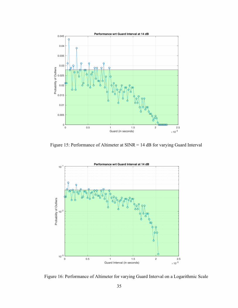
35
Figure 15: Performance of Altimeter at SINR = 14 dB for varying Guard Interval
Figure 16: Performance of Altimeter for varying Guard Interval on a Logarithmic Scale
0 0.5 1 1.5 2 2.5Guard (in seconds) 10-3
0
0.005
0.01
0.015
0.02
0.025
0.03
0.035
0.04
0.045
Prob
abilit
y of
Out
liers
Performance wrt Guard Interval at 14 dB
0 0.5 1 1.5 2 2.5Guard Interval (in seconds) 10-3
10-3
10-2
10-1
Prob
abilit
y of
Out
liers
Performance wrt Guard Interval at 14 dB

36
It is evident that the performance of this technique depends heavily on the timing module
in both the systems. However, timing synchronization is a mature technology and thus, this
requirement could be fulfilled using a variety of off-the-shelf products.
Table 4 comprises of the number of outliers (errors due to interference) observed for
different techniques at different SINR.
Table 4: Number of Outliers observed for different Interference Mitigation Techniques
SINR
(in dB)
Interference
Power (in
dB)
Number of Outliers (out of 1000)
Absence of IM
Techniques
Spectral
Shaping
Spread
Spectrum
Time
Suppressed IC
14 45.989 57 67 91 22
14.5 44.921 33 29 29 6
15 43.681 10 10 14 3
15.5 42.164 3 3 1 4
16 40.142 0 0 0 0
16.5 36.874 0 1 0 0
17 N/A 0 0 0 0

37
CHAPTER IV
CONCLUSION
It is possible to establish a secondary wireless system (WAIC) in the same frequency band as the
one currently being utilized by commercial altimeters, without causing any disruption to the
altimeters by incorporating good interference management techniques like the Time-Synchronized
IM technique.

38
REFERENCES
1. Canaday, H., 2017, May. War on Wiring. Aerospace America. AIAA.
2. http://focusnews.co/a380-wiring-diagram.html
3. Yelverton, J.N., 1995, November. Wireless avionics. In Digital Avionics Systems
Conference, 1995., 14th DASC (pp. 95-99). IEEE.
4. Elliott K., 2017, June/July. Development of Wireless Avionics Intra-Communications.
Avionics Digital. Aviation Today.
5. 2015, Feb. RECOMMENDATION ITU-R M.2067-0, Technical characteristics and
protection criteria for Wireless Avionics Intra- Communication systems
6. 2013, Dec. REPORT ITU-R M.2283-0, Technical characteristics and spectrum
requirements of Wireless Avionics Intra-Communications systems to support their safe
operation
7. Bellamy III W., 2014, September. Aircraft Wire and Cable: Doing More With Less.
Avionics International. Aviation Today.
8. https://aviation.stackexchange.com/questions/2263/what-is-the-lifespan-of-commercial-
airframes-in-general
9. Dang, D.K., Mifdaoui, A. and Gayraud, T., 2012. Fly-by-wireless for next generation
aircraft: Challenges and potential solutions.
10. Sámano-Robles, R., Tovar, E., Cintra, J. and Rocha, A., 2016, September. Wireless
avionics intra-communications: Current trends and design issues. In Digital Information
Management (ICDIM), 2016 Eleventh International Conference on (pp. 266-273). IEEE.

39
11. Raharya, N. and Suryanegara, M., 2014, August. Compatibility analysis of Wireless
Avionics Intra Communications (WAIC) to radio altimeter at 4200–4400 MHz. In Wireless
and Mobile, 2014 IEEE Asia Pacific Conference on (pp. 17-22). IEEE.
12. 2014, Nov. REPORT ITU-R M.2318-0, Consideration of the aeronautical mobile (route),
aeronautical mobile, and aeronautical radionavigation services allocations to accommodate
wireless avionics intra-communication
13. Suryanegara, M., Nashirudin, A., Raharya, N. and Asvial, M., 2015, December. The
compatibility model between the Wireless Avionics Intra-Communications (WAIC) and
fixed services at 22-23 GHz. In Aerospace Electronics and Remote Sensing Technology
(ICARES), 2015 IEEE International Conference on (pp. 1-5). IEEE.
14. 2014, Feb. RECOMMENDATION ITU-R M.2059-0, Operational and technical
characteristics and protection criteria of radio altimeters utilizing the band 4 200-4 400
MHz
15. Hanschke, L., Krüger, L., Meyerhoff, T., Renner, C. and Timm-Giel, A., 2017, May. Radio
altimeter interference mitigation in wireless avionics intra-communication networks.
In Modeling and Optimization in Mobile, Ad Hoc, and Wireless Networks (WiOpt), 2017
15th International Symposium on (pp. 1-8). IEEE.
16. 2014, Nov. REPORT ITU-R M.2319-0, Compatibility analysis between wireless avionic
intra-communication systems and systems in the existing services in the frequency band 4
200-4 400 MHz
17. Meyerhoff, T., Faerber, H. and Schwark, U., 2015, February. Interference Impact of
Wireless Avionics Intra-Communication Systems onto Aeronautical Radio Altimeters.

40
In SCC 2015; 10th International ITG Conference on Systems, Communications and
Coding; Proceedings of (pp. 1-6). VDE.
18. ITU Radio Regulations, Section IV. Radio Stations and Systems – Article 1.108,
definition: radio altimeter
19. https://en.wikipedia.org/wiki/Radar_altimeter
20. Vidmar, M., 2006, August. A landing radio altimeter for small aircraft. In Power
Electronics and Motion Control Conference, 2006. EPE-PEMC 2006. 12th
International (pp. 2020-2024). IEEE.
21. "COMMENTS OF AVIATION SPECTRUM RESOURCES, INC.". p. 3, p. 8.
22. http://www.radartutorial.eu/02.basics/Frequency%20Modulated%20Continuous%20Wav
e%20Radar.en.html
23. https://en.wikipedia.org/wiki/Chirp
24. https://en.wikipedia.org/wiki/Johnson–Nyquist_noise
25. Hong, X., Chen, Z., Wang, C.X., Vorobyov, S.A. and Thompson, J.S., 2009. Cognitive
radio networks. IEEE vehicular technology magazine, 4(4).
26. Yucek, T. and Arslan, H., 2009. A survey of spectrum sensing algorithms for cognitive
radio applications. IEEE communications surveys & tutorials, 11(1), pp.116-130.
27. Aparna, P.S. and Jayasheela, M., 2012. Cyclostationary feature detection in cognitive radio
using different modulation schemes. International Journal of Computer
Applications, 47(21).