Interference from Large Wireless Networks

under Correlated Shadowing

by

Sebastian S. Szyszkowicz, B.A.Sc., M.A.Sc.

A thesis submitted to The Faculty of Graduate and Postdoctoral Affairs

in partial fulfillment of the requirements for the degree of

Doctor of Philosophy in Electrical and Computer Engineering

Ottawa–Carleton Institute for Electrical and Computer Engineering (OCIECE)

Department of Systems and Computer Engineering

Carleton University

Ottawa, Ontario, Canada, K1S 5B6

January 2011

c⃝ Copyright 2011, Sebastian S. Szyszkowicz

The undersigned recommend to

the Faculty of Graduate and Postdoctoral Affairs

acceptance of the thesis

Interference from Large Wireless Networks under Correlated Shadowing

submitted by

Sebastian S. Szyszkowicz, M.A.Sc., B.A.Sc.

in partial fulfilment of the requirements for

the degree of Doctor of Philosophy in Electrical and Computer Engineering

Chair, Howard Schwartz, Department of Systems and Computer Engineering

Thesis Supervisor, Halim Yanıkomeroglu

External Examiner, Jacek I low, Department of Electrical and Computer

Engineering, Dalhousie University, Halifax, Canada

Carleton University

January 2011

Abstract

We study the statistical distribution of the total interference power caused by a large

wireless network and aggregated at a single victim receiver. We show that correlation

between shadowing paths becomes a dominating factor in the interference from large

networks, and should not be neglected. We thus propose a new problem formulation,

which may include any pathloss, interferer distribution, and shadowing spread and

correlation model. We make an extensive study of the existing correlation models for

shadowing, and identify one that has the most desirable mathematical and physical

characteristics. We then formulate a two–fold solution to the problem of finding the

total interference distribution. We first develop an analytically–tractable approxi-

mation that applies to a subset of the interference scenarios. In order to solve the

problem more generally, we then propose a reformulation in three steps of the sim-

ulation algorithm that achieve time gains of the order of 1000, with minimal loss in

accuracy. These two approaches allow us to solve a highly computationally intensive

problem in seconds, not hours, on a personal computer. The algorithms are validated

by via direct Monte Carlo simulations.

The problem is of great interest for enabling aggressive channel reuse and hetero-

geneous network coexistence in future wireless systems, where interference is expected

to be the dominating factor.

iii

Acknowledgements

To my supervisor and hocam1, Dr. Halim Yanıkomeroglu, for his endless support,

patience, encouragement, and indeed friendship. I could not have wished for a better

supervisor.

My sincere gratitude goes towards my thesis examiners:

• Prof. Paul C. Johns (Committee Chair), Dept. Physics, Carleton University,

• Prof. Jacek I low (External Examiner), Dept. Electrical and Computer Engi-

neering, Dalhousie University, Halifax,

• Prof. Yiqiang Zhao, School of Mathematics and Statistics, Carleton University,

• Prof. Abbas Yongacoglu, School of Information Technology and Engineering,

University of Ottawa,

• Prof. Ioannis Lambadaris, Dept. Systems and Computer Engineering, Carleton

University,

for carefully reviewing my work and giving me valuable comments towards the im-

provement of this thesis, as well as for a very pleasant defence experience.

Thank you to my colleagues in our group and department for the technical dis-

cussions as well as the lighter moments. You have made my time at Carleton both

enjoyable and instructive. My thanks in particular to Furkan Alaca and Arshdeep

1hocam: “my teacher”, honorific (Turkish)

iv

S. Kahlon, whom I have had the pleasure to mentor and work with, and who have

taught me a great deal in their turn.

My thanks go to the many researchers with whom I had the honour to interact

during the course of my graduate studies, for their hospitality and warmth during my

travel visits, and for many interesting and enlightening technical discussions, which

deepened my understanding of many topics, and helped sharpen several ideas in this

thesis. Most notably, I would like to thank Prof. John S. Thompson, University

of Edinburgh, Scotland, UK, for his generosity and friendliness in hosting me as a

visiting researcher in the winter of 2008, and from a valuable research collaboration

therefrom.

I would also like to thank the ladies of our department office, for their generous

and courteous help in navigating the administrative aspects of academic life. My

gratitude also goes towards the gentlemen in our technical staff for their competent

and patient help with all my computing needs. My thanks also go to the members

of the cleaning and support staff here in the Minto CASE building, for providing me

with a clean and functional working environment.

To my good friends far and near, you who make life light to bear, you who know

the good and the bad of me2. Thank you for being there for me through thick and

thin, for sharing in my joys and sorrows, for rejoicing in my successes and for helping

me recover from my failures. My thanks in particular go to Nick Milne, for his

courageous proofreading of this entire thesis.

Thank you to my parents, Barbara and Mieczys law, for the gift of life, for their

many sacrifices for me, for teaching me many of the most important things. A big

hug to my little sister Kasia for always being there to cheer me up and for preventing

me from taking myself too seriously. You make me very proud!

2“Friends are those with whom our faults are safe.” — G. K. Chesterton

v

In the beginning was the Word, and the Word was with God, and the Word was

God. [...] And the Word was made flesh, and dwelt among us.

— The Gospel of John

vi

Contents

Abstract iii

Acknowledgements iv

Contents vii

List of Figures xiii

List of Tables xvi

Nomenclature xvii

1 Introduction 1

1.1 Motivation for this Research . . . . . . . . . . . . . . . . . . . . . . . 2

1.2 Positioning our Work with Respect to Current Literature . . . . . . . 4

1.2.1 Sums of Lognormal Random Variables . . . . . . . . . . . . . 4

1.2.2 Interference from Poisson Fields . . . . . . . . . . . . . . . . . 6

1.2.3 Correlated Shadowing through Shadowing Fields . . . . . . . . 7

1.2.4 Our Work as a Synthesis of these Lines of Research . . . . . . 8

1.3 Plan of the Thesis . . . . . . . . . . . . . . . . . . . . . . . . . . . . . 10

1.4 Mathematical Tools . . . . . . . . . . . . . . . . . . . . . . . . . . . . 12

1.4.1 Linear Algebra . . . . . . . . . . . . . . . . . . . . . . . . . . 12

1.4.2 Gaussian Random Variables and Processes . . . . . . . . . . . 13

vii

1.4.3 Convergence of Random Variables . . . . . . . . . . . . . . . . 15

1.4.4 Exchangeable Random Variables . . . . . . . . . . . . . . . . 16

2 Choosing a Good Shadowing Correlation Model 18

2.1 Types of Correlation . . . . . . . . . . . . . . . . . . . . . . . . . . . 20

2.1.1 Scenarios . . . . . . . . . . . . . . . . . . . . . . . . . . . . . 20

2.1.2 Auto–Correlation . . . . . . . . . . . . . . . . . . . . . . . . . 21

2.1.3 Cross–Correlation . . . . . . . . . . . . . . . . . . . . . . . . . 22

2.1.4 Mathematical Synthesis of Auto– and Cross–Correlation . . . 22

2.1.5 Generalised Correlation . . . . . . . . . . . . . . . . . . . . . 23

2.1.6 Time–Correlation . . . . . . . . . . . . . . . . . . . . . . . . . 24

2.1.7 Uplink–Downlink Correlation . . . . . . . . . . . . . . . . . . 24

2.2 Positive Semidefiniteness of Correlation Models . . . . . . . . . . . . 25

2.2.1 Models with Variable Shadowing Variance . . . . . . . . . . . 25

2.2.2 Methods for Proving Positive Semidefiniteness . . . . . . . . . 26

2.2.3 One–Parameter and Separable Correlation . . . . . . . . . . . 27

2.2.4 Incorporating Time and Uplink–Downlink Correlation . . . . . 28

2.3 Estimating the Correlation Function from Measured Data . . . . . . . 31

2.3.1 Auto–Correlation as Mixed Time–Space Measurements . . . . 31

2.3.2 Cross–Correlation as Spatial–Only Correlation . . . . . . . . . 32

2.3.3 Collapsing Correlation onto One Dimension . . . . . . . . . . 33

2.4 Specific Correlation Models and Their Positive Semidefiniteness . . . 34

2.4.1 Constant Model . . . . . . . . . . . . . . . . . . . . . . . . . . 34

2.4.2 Absolute Distance–Only Models . . . . . . . . . . . . . . . . . 35

2.4.2.1 Exponential Model . . . . . . . . . . . . . . . . . . . 36

2.4.2.2 More Complex Models . . . . . . . . . . . . . . . . . 37

2.4.3 Angle–Only Models . . . . . . . . . . . . . . . . . . . . . . . . 38

viii

2.4.4 Separable Models . . . . . . . . . . . . . . . . . . . . . . . . . 40

2.4.4.1 Angle–Distance Ratio . . . . . . . . . . . . . . . . . 41

2.4.4.2 Angle–Absolute Distance . . . . . . . . . . . . . . . 42

2.4.5 More Elaborate (Non–Separable) Models . . . . . . . . . . . . 43

2.5 Some Thoughts on Physical Realism . . . . . . . . . . . . . . . . . . 45

2.6 Feasibility According to Marginal Distribution . . . . . . . . . . . . . 49

2.6.1 Jointly Lognormal Shadowing . . . . . . . . . . . . . . . . . . 49

2.6.2 Non–Lognormal Shadowing . . . . . . . . . . . . . . . . . . . 49

2.7 Consequences for Working with Correlated Shadowing . . . . . . . . . 50

2.7.1 For Those Wanting to Incorporate Shadowing Correlation . . 51

2.7.2 For Those Using a Model that Is Not Feasible . . . . . . . . . 51

2.7.3 For Those Designing New Correlation Models . . . . . . . . . 51

2.7.4 For Those Studying Large Interference Problems . . . . . . . . 52

3 Problem Statement 53

3.1 Interferer Layout . . . . . . . . . . . . . . . . . . . . . . . . . . . . . 53

3.1.1 Poisson Field . . . . . . . . . . . . . . . . . . . . . . . . . . . 53

3.1.2 Weighed Spatial Distribution . . . . . . . . . . . . . . . . . . 54

3.1.3 Cluster Layouts . . . . . . . . . . . . . . . . . . . . . . . . . . 55

3.1.4 Layout Examples . . . . . . . . . . . . . . . . . . . . . . . . . 55

3.2 Channel Models . . . . . . . . . . . . . . . . . . . . . . . . . . . . . . 57

3.2.1 Average Pathloss . . . . . . . . . . . . . . . . . . . . . . . . . 57

3.2.2 Lognormal Shadowing . . . . . . . . . . . . . . . . . . . . . . 58

3.2.3 Spatially–Correlated Jointly Lognormal Shadowing . . . . . . 58

3.3 Interferer Transmission . . . . . . . . . . . . . . . . . . . . . . . . . . 60

3.4 Total Interference . . . . . . . . . . . . . . . . . . . . . . . . . . . . . 60

ix

4 Analytical Results on the Aggregate Interference 63

4.1 Approximate Solution using Exchangeability . . . . . . . . . . . . . . 63

4.1.1 Limit Theorem on the Sum of Exchangeable Joint Lognormals 64

4.1.1.1 Problem Formulation . . . . . . . . . . . . . . . . . . 64

4.1.1.2 Main Result and Proof . . . . . . . . . . . . . . . . . 65

4.1.1.3 Lognormal Approximation for Large N . . . . . . . . 66

4.1.2 Lognormal Approximation to Total Interference Distribution . 67

4.1.2.1 Comparing the Two Problems . . . . . . . . . . . . . 67

4.1.2.2 Cross–Moment–Matching between the Two Problems 70

4.1.2.3 Simple Semi–Analytical Solution . . . . . . . . . . . 71

4.2 Study of Moments . . . . . . . . . . . . . . . . . . . . . . . . . . . . 73

4.2.1 Formulation of Moments . . . . . . . . . . . . . . . . . . . . . 73

4.2.2 Numerical Evaluation of Moments . . . . . . . . . . . . . . . . 74

4.2.3 Using Moments in the Large–N Regime . . . . . . . . . . . . 75

4.2.3.1 Mean–Matching . . . . . . . . . . . . . . . . . . . . . 76

4.2.3.2 Variance–Matching . . . . . . . . . . . . . . . . . . . 76

4.2.3.3 Matching both Mean and Variance . . . . . . . . . . 77

4.3 Problem Reformulation Using a Stochastic Integral . . . . . . . . . . 78

4.3.1 Equivalent Stochastic Integral for I/N as N → ∞ . . . . . . . 79

4.3.2 Mathematical Argument . . . . . . . . . . . . . . . . . . . . . 79

4.4 Summary . . . . . . . . . . . . . . . . . . . . . . . . . . . . . . . . . 80

5 Simulation Results and Optimisation 81

5.1 Simulation Setup . . . . . . . . . . . . . . . . . . . . . . . . . . . . . 81

5.1.1 Simulation Platform . . . . . . . . . . . . . . . . . . . . . . . 81

5.1.2 Traditional Approach: Matrix Factorisation . . . . . . . . . . 82

5.1.3 Representing the Simulation Results . . . . . . . . . . . . . . 84

x

5.1.4 Correlated versus Independent Shadowing . . . . . . . . . . . 86

5.2 Evaluating the Accuracy of the Lognormal Approximation Method . 86

5.2.1 Accuracy of Convergence of the SEJLN Distribution to the Log-

normal . . . . . . . . . . . . . . . . . . . . . . . . . . . . . . . 86

5.2.2 Numerical Evaluation of the Geometric Coefficients . . . . . . 94

5.2.3 Lognormal Approximation to I in a Clustered Layout . . . . . 96

5.2.4 Lognormal Approximation to I in a Non–Clustered Layout . . 96

5.3 Simulating I Rapidly: Combined Simulation–Numerical–Analytical Ap-

proach . . . . . . . . . . . . . . . . . . . . . . . . . . . . . . . . . . . 103

5.3.1 Shadowing Fields . . . . . . . . . . . . . . . . . . . . . . . . . 105

5.3.2 Efficient Filtering for Separable Triangular Correlations . . . . 109

5.3.2.1 Separability . . . . . . . . . . . . . . . . . . . . . . . 109

5.3.2.2 Optimised Box Filters . . . . . . . . . . . . . . . . . 109

5.3.2.3 Optimised Shadow Fields Algorithm . . . . . . . . . 109

5.3.3 Reusing Random Samples . . . . . . . . . . . . . . . . . . . . 111

5.3.3.1 Reuse in Matrix Factorisation . . . . . . . . . . . . . 112

5.3.3.2 Reuse in Shadowing Fields . . . . . . . . . . . . . . . 113

5.3.4 Simulator Calibration . . . . . . . . . . . . . . . . . . . . . . . 114

5.3.5 Time Performance Comparison . . . . . . . . . . . . . . . . . 119

5.3.6 Moment–Corrected Extrapolations for High N . . . . . . . . . 121

5.3.7 Optimising Other Correlation Models . . . . . . . . . . . . . 127

6 Conclusion and Future Work 128

6.1 Achievements of this Thesis . . . . . . . . . . . . . . . . . . . . . . . 128

6.2 Immediate Model Extensions . . . . . . . . . . . . . . . . . . . . . . . 131

6.2.1 Random Number of Interferers . . . . . . . . . . . . . . . . . . 131

6.2.2 Non–Independent Interferer Positions . . . . . . . . . . . . . . 133

xi

6.2.3 Small–Scale Fading and Variable Interferer Transmit Power . . 133

6.2.4 Directional Victim Receiver Antenna . . . . . . . . . . . . . . 135

6.2.5 Other Dimensions: Time and Frequency . . . . . . . . . . . . 136

6.3 Long–Term Research Questions . . . . . . . . . . . . . . . . . . . . . 137

Bibliography 140

xii

List of Figures

1.1 Plan of thesis argument, with corresponding sections and publications. 10

2.1 a) Shadowing auto–correlation for a mobile Y (t), b) Shadowing cross–

correlation for a mobile X. . . . . . . . . . . . . . . . . . . . . . . . . 21

2.2 Generic geometry of shadowing auto– and cross–correlation. . . . . . 23

2.3 A pair of auto– or cross–correlated paths, with the most relevant di-

mensional variables: d, θ, R. . . . . . . . . . . . . . . . . . . . . . . . 33

2.4 Shadowing correlation model families according to physical dimensions

described in Figure 2.3. Other parameter combinations are possible but

have not been encountered in literature. . . . . . . . . . . . . . . . . 35

2.5 Physical argument of common propagation area for correlation in shad-

owing. . . . . . . . . . . . . . . . . . . . . . . . . . . . . . . . . . . . 48

3.1 Interferer layouts used in this thesis. Distances are in meters. . . . . . 56

3.2 Shadowing correlation function (3.5) with θ0 = 60◦ and R0 = 6 dB:

the correlation coefficient between two shadowed paths beginning at

base of the arrow. One path ends at the tip of the arrow, while the

other is located anywhere on the plane. The figure is invariant under

rotation and scaling. . . . . . . . . . . . . . . . . . . . . . . . . . . . 61

5.1 Interference cdfs on lognormal paper: with and without shadowing

correlation. . . . . . . . . . . . . . . . . . . . . . . . . . . . . . . . . 85

xiii

5.2 SEJLN cdf on lognormal paper, σ = 6 dB, ρ = 0.5, with varying N . . 88

5.3 SEJLN cdf on lognormal paper, σ = 6 dB, ρ = 0.05, with varying N . 89

5.4 SEJLN cdf on lognormal paper, σ = 6 dB, ρ = 0.005, with varying N . 90

5.5 SEJLN cdf on lognormal paper, σ = 12 dB, ρ = 0.5, with varying N . 91

5.6 SEJLN cdf on lognormal paper, σ = 12 dB, ρ = 0.05, with varying N . 92

5.7 SEJLN cdf on lognormal paper, σ = 12 dB, ρ = 0.005, with varying N . 93

5.8 Total interference cdf on lognormal paper for Layout A, with σs = 6 dB,

β = 4, and N = 1, 10, 100, 1000 from left to right. . . . . . . . . . . . 97

5.9 Total interference cdf on lognormal paper for Layout A, with σs =

12 dB, β = 3, and N = 1, 10, 100, 1000 from left to right. . . . . . . . 98

5.10 Total interference cdf on lognormal paper for Layout B, with σs = 6 dB,

β = 3, and N = 1, 10, 100, 1000 from left to right. . . . . . . . . . . . 99

5.11 Total interference cdf on lognormal paper for Layout B, with σs =

12 dB, β = 4, and N = 1, 10, 100, 1000 from left to right. . . . . . . . 100

5.12 Total interference cdf on lognormal paper for Layout C, with σs = 6 dB,

β = 4, and N = 1, 10, 100, 1000 from left to right. . . . . . . . . . . . 101

5.13 Total interference cdf on lognormal paper for Layout D, with σs = 6 dB,

β = 4, and N = 1, 10, 100, 1000 from left to right. . . . . . . . . . . . 102

5.14 Shadowing field realisations for rmin = 50, rmax = 500, θ0 = 60◦, R0 =

6 dB, with increasing resolution: DΘ = 6n,DR = 5n, FΘ = n, FR = 3n,

where a) n = 1, b) n = 2, c) n = 5, d) n = 50. The colour of the areas

corresponds to the value of Si/σs(ri) therein. . . . . . . . . . . . . . . 106

5.15 Calibration of field resolution parameters DΘ = 6n and DR = 5n, and

the resulting simulated cdfs of I. . . . . . . . . . . . . . . . . . . . . 116

5.16 Effect of random sample reuse in matrix factorisation algorithm on the

cdf of I. K = 1 000 000, Kr = KCh = K/m. . . . . . . . . . . . . . . . 117

xiv

5.17 Effect of combining random sample reuse with calibrated (DΘ = 12, DR =

10) shadowing fields algorithm on the cdf of I. K = 1 000 000, Kr =

KCh = K/m. . . . . . . . . . . . . . . . . . . . . . . . . . . . . . . . 118

5.18 Execution time performance of matrix (Cholesky) factorisation versus

shadowing fields, and of no reuse versus random sample reuse. Simu-

lation parameters are given in Table 5.2. . . . . . . . . . . . . . . . . 120

5.19 Using mean–matching (4.24) to extrapolate the cdf of I for very high

N . All simulations are done using shadowing fields with reuse. . . . . 123

5.20 Using variance–matching (4.26) to extrapolate the cdf of I for very

high N . All simulations are done using shadowing fields with reuse. . 124

5.21 Using two–moment–matching (4.31) to extrapolate the cdf of I for very

high N . All simulations are done using shadowing fields with reuse. . 125

xv

List of Tables

2.1 Summary of existing shadowing correlation models and their properties. 46

5.1 Geometric coefficients for each layout in Figure 3.1. . . . . . . . . . . 94

5.2 Simulation settings after calibration. . . . . . . . . . . . . . . . . . . 104

xvi

Nomenclature

Acronyms

Acronym Meaning

cdf cumulative distribution function

CLT central limit theorem

FFT fast Fourier transform

iid independent and identically distributed

IS interfering station

LLN law of large numbers

pdf probability density function

PPP Poisson point process

psd positive semidefinite

RP random process

RV random variable

RX victim receiver station

SEJLN sum of exchangeable joint lognormals

xvii

Mathematical Operators and Symbols

Notation Meaning

∗ convolution

[Xi]Ni=1 vector of elements X1, X2, . . . , XN

{Xi}Ni=1 set of elements X1, X2, . . . , XN

|S| “natural” measure of set S, e.g., area, volume, etc.

A \ B set subtraction: the set of elements in A not in BC = A× B Cartesian product of sets: x ∈ A, y ∈ B ⇒ (x, y) ∈ Cf : A 7→ B f is a mapping from the set A to the set B.

f : x 7→ y f maps x to y.

XD−→ Y RV X converges in distribution to RV Y .

XD= Y RV X and RV Y have the same distribution.

XD≈ Y RV X and RV Y have approximately the same distribution.

A|B statistical conditioning of A given B (of RVs or events)

[xi,j]M×N matrix composed of entries xi,j with indices i = 1, . . . ,M, j =1, . . . , N

AT the matrix (or vector) transpose of A∗√K any N × N matrix decomposition of N × N matrix K such that

∗√K ∗√K

T= K

◦ Hadamard/Schur matrix product

⊗ Kronecker/Zehfuss matrix product

diag(x1, . . . , xN) square matrix with entries x1, . . . , xN on the main diagonal, andzero elsewhere

E {X} expected value of RV X

N∗ the set of natural numbers (excluding zero)

N (µ,K) jointly–Gaussian (normal) distribution with mean vector µ and co-variance matrix K

O(f(N)) order of f(N), “Big–O” notation

P (E) probability of event E occurring

Φ(x) standard Gaussian cdf

R the set of real numbers

xviii

R+ the set of non–negative real numbers (including zero)

RX(τ) autocorrelation function of stationary process X(t) (can be ex-tended to random fields)

VAR {X} variance of RV X

Z the set of integers

xix

Physical and Mathematical Quantities

Symbol Meaning

A, B, C moments and cross–moments of Ii

a, b, c, a′, b′, c′ scaling coefficients for extrapolation to larger N

A square region in stochastic integral argument, that entirely containsAg

Ag entire region where g is non-zero

Al sub–square region of Aβ pathloss exponent when average pathloss is power–law

C N ×N matrix such that CCT = K, if it exists

DR length of discrete shadowing field in the R dimension

DΘ length of discrete shadowing field in the θ dimension

d Cartesian distance between two points, used in shadowing correla-tion models

dm distance covered by a mobile at time t when considering shadowingmeasurements

δ side length of square Aηx(ξ)ηy(υ) separable auto–correlation function of M

F discrete filter kernel for generating M, of size FR × FΘ

FR length of discrete shadowing field filter in the R dimension

FΘ length of discrete shadowing field filter in the θ dimension

g(r) two–dimensional pdf of IS locations ri

g(r) pdf of ri derived from g(r)

G1, G2 constants obtained by integration over g()

Gcor constant obtained by integration over g() and h()

H correlation coefficient matrix of S, formed by [h(r1, r2)]N×N

h(r1, r2) shadowing correlation model

h(r1, r2) true physical shadowing correlation function

h(r1, r2) estimated physical shadowing correlation function

h(r1, r2) shadowing correlation model for the return paths of those ofh(r1, r2)

xx

hd(d) correlation model along the d dimension, when h is thus separable

hR(R) correlation model along the R dimension, when h is thus separable

hΘ(θ) correlation model along the θ dimension, when h is thus separable

I total interference power at the RX from all ISs

Ii interference power at the RX from IS i

Jl binomial RV representing the number of points falling in square Al

J0(x) Bessel function of the first kind

K covariance matrix of S

K expanded covariance matrix of shadowing, given points in time,space, and both path directions

K number of trials of I generated in Monte Carlo simulations

KCh number of trials of S

Kr number of trials of [ri]Ni=1

λ constant equal to 0.1 ln 10 ≈ 0.2303, used to convert between expo-nentials and dB

λP density of a Poisson point process

M discrete version of M

M continuous stationary field representing the shadowing field undera geometric transformation

M scaling factor for the number of ISs, used in extrapolation

m reuse factor, defined when KCh = Kr

mV mean parameter of lognormal RV approximating the SEJLN RV V

m∞ mean parameter of limiting lognormal RV of V/N as N → ∞µ mean coefficient in the SEJLN distribution

N number of ISs (a non–random value)

p(r) average pathloss function

ql length of ql

ql position of centre of square Al

R distance ratio in dB, used in shadowing correlation models

R0 distance ratio parameter in correlation model (3.5)

RS(τ) auto–correlation function of S(t), Si(t), and Si(t)

xxi

ri two–dimensional vector giving the position of IS i, randomly dis-tributed according to g

ri length of ri

∠ri angle of ri

rmax largest value that ri can take for a given g()

rmin smallest value that ri can take for a given g()

ρ correlation coefficient in the SEJLN distribution

ρi,j correlation coefficient between Si and Sj

ρud Uplink–Downlink correlation coefficient: correlation between theshadowing on a path and that on its return path

S the vector of shadowing terms: [Si]Ni=1

Si natural logarithm of shadowing power gain on propagation pathbetween IS i and the RX, with distribution N (0, σ2

s )

S(r) shadowing field in two dimensions

S(t), Si(t) shadowing process in time

Si(t) shadowing process in time on the return path of that of Si(t)

sV spread parameter of lognormal RV approximating the SEJLN RVV

s∞ spread parameter of limiting lognormal RV of V/N as N → ∞s vector of shadowing standard deviations: [σs(ri)]

Ni=1

s combined vector of shadowing standard deviations in both pathdirections

σ standard deviation coefficient (in natural units) in the SEJLN dis-tribution

σi = σs(ri) shadowing spread in dB as a function of position (usually onlydistance), may be constant

σi = σs(ri) shadowing spread in dB on the return path of that of σi

σs shadowing spread in dB, when independent of distance

TLP log–polar geometric mapping

t, ti time instant when considering a shadowing scenario evolving intime

θ minimum angle (≤ 180◦), used in shadowing correlation models

θ0 angle parameter in correlation model (3.5)

xxii

v speed of a mobile, equal to ∥v∥v velocity vector of a mobile when considering shadowing measure-

ments

V SEJLN RV

Vi exchangeable jointly Gaussian RVs

W common shadowing component of S1 and S2

Wi shadowing component exclusively of Si

w2, w21 and w2

2 variances of W , W1, and W2, respectively

X, Xi, Y , Yi endpoints of propagation paths−−→XY a directed propagation path from point X to point Y

Z, Zi independent standard Gaussian RVs

Z vector of iid standard Gaussian RVs

z vector of the inverse of shadowing standard deviations: [σ−1s (ri)]

Ni=1

ζ(τ) normalised auto–correlation function of S(t), Si(t), and Si(t)

Section 2.4 also describes a series of existing shadowing models whose parameter

names are often taken directly from literature and should not be confused with the

above notations. These parameters are only used in that section and in Table 2.1,

and pertain only to the model in which they are used. These are: A, a (multiple

times), α (multiple times), B, b (multiple times), d0, d1, d2, dsep, d, γ, K, ν, ρ, θT.

xxiii

Chapter 1

Introduction

This thesis is about aggregate interference power at a victim receiver, and about

spatial correlation in wireless shadowing, two established lines of research in the

wireless community. The purpose of this thesis is four–fold:

1. To demonstrate that shadowing correlation is indeed very important in large

interference scenarios, and cannot be realistically ignored.

2. To develop a problem formulation that is a synthesis of many scenarios studied

in literature: a problem that is realistic and general enough to cover the widest

possible set of real interference scenarios, while still being tractable in some

way.

3. To obtain the statistical distribution of this aggregate interference from a large

number of interferers, in a manner that is accurate, computationally efficient,

and easy to understand and implement in simulations.

4. To properly choose a shadowing correlation model and to implement it efficiently

in a simulation platform.

The problem is of significant importance: the aggressive reuse of precious wireless

spectrum needed to achieve futuristic wireless throughputs will require a very good

theoretical understanding of heavy interference scenarios.

1

1.1 Motivation for this Research

The number of wireless devices, both for personal use and for autonomous machine

applications, is likely to grow in the near future. Indeed, if we include autonomous

devices such as wireless sensors, there is the potential for even trillions of devices

in the upcoming years [1]. The wireless spectrum, however, remains scarce, and an

aggressive spatial frequency reuse will likely be necessary. Several recent works [2, 3]

have taken an interest in practical interference scenarios, where the number of inter-

ferers is more than 100. The nature of the interfering nodes may be femtocells [2],

sensor nodes, or any other devices that aggressively share spectrum, often in a non–

coordinated and opportunistic manner. This type of scenario is becoming increasingly

relevant as wireless communications move away from the traditional coordinated cel-

lular model to more heterogeneous and distributed paradigms, such as ad–hoc net-

working and cognitive radio [3, 4]. There is also potential for application in cellular

systems that are augmented by a large number of autonomous devices, such as no-

madic relays [5]. Thus the study of interference from many co–channel interferers

is essential for the design of future wireless systems. The immediate implication

for wireless networks will be heavy co–channel interference, particularly in densely–

populated (urban) scenarios, and perhaps in massively–deployed sensor networks as

well. It is likely that many wireless systems will be interference–limited, with co–

channel interference originating from very many wireless transmitters, and that the

signal–to–interference ratio statistics will be an important performance metric. A

good understanding of these interference scenarios will therefore be crucial in future

wireless network planning.

It can be argued, however, that the state of literature on interference problems

is not currently prepared to appropriately model these large numbers of interferers.

On the side of analytical and numerical approaches, we have one of two situations:

2

either very accurate results for small numbers of interferers, but that scale poorly for

large networks; or analysis of large fields of wireless interferers, but this with very

restrictive and simplistic channel and system models that may not at all correspond to

most real scenarios. A synthesis of these two approaches is therefore in order. Several

works [4, 6–11] have considered large interfering networks with independent received

interfering signals and concluded that the total received interference is approximately

Gaussian, by application of the central limit theorem (CLT). The problem, however,

is not so simple. Indeed, adding correlation produces very different results, as we show

in this thesis, and therefore we propose our work as an improvement in accuracy over

the CLT approach.

Furthermore, as computational power is increasing, we believe that the benefits

of analysing small systems are waning, as most can be simulated via some Monte

Carlo approach in good–enough time. This is not at all the case for large networks,

where computational time and memory may become prohibitive. Such problems

instead benefit from either an asymptotic analysis or a judicious reformulation of the

problem that is less sensitive to the number of devices.

Finally, there exists a risk of a certain disjoint between theoretical results in the

academic world, and results of practical value for vendors and network operators (this

wide–ranging problem is addressed in [1,12]). We therefore emphasise the importance

of developing results that are of practical use to designers: specifically, we want to

provide a method that solves the problem at hand accurately, and with minimal

human and computer resources. Apart from these goals, we want to solve the problem

“by any means necessary”, and we feel that a judicious mixture of analysis, numerical

techniques, and Monte Carlo simulation might be the best solution to the problem at

hand (this may be the case for many other problems also).

In this thesis, we follow these lines of thought to formulate

• a new problem that is very general, difficult and important to solve, while being

3

useful in future interference scenarios,

• a set of solutions that benefit from accuracy, ease of implementation, and min-

imal computational effort.

1.2 Positioning ourWork with Respect to Current Literature

The problem that we formulate and partly solve in this thesis has not been addressed

before. Rather it lies at the intersection of three research arcs, of which the first two

represent a significant portion of the work on wireless interference in recent years. We

examine each sub–field in turn, note its strengths and weaknesses, and then explain

how our work synthesises these approaches to produce a more realistic, general, and

efficiently solvable problem.

1.2.1 Sums of Lognormal Random Variables

The problem of finding the distribution of the sum of several lognormal random

variables (RVs) is a long–standing mathematical problem in the wireless commu-

nity [13], and has received renewed interest since around 2004. We made a study of

the proposed solutions in our Masters thesis [14] concerning pre–2007 literature, and

produced some results of our own [15, 16]. Since then, there have been significant

advances in this field, notably [17–23].

The sum of lognormals approach is based on the idea that the interference ar-

riving at the victim receiver station (RX) from any one interfering station (IS) is

(approximately) lognormally distributed, given a significant shadowing component, a

lesser (or ignored) effect from small–scale fading, and little or no statistical variabil-

ity of the positions (which, through pathloss, affect the log–mean of the lognormal

distributions). Furthermore, several of the new methods consider correlation between

shadowing paths [20, 23] (as well as [17, 21], which only study the tail behaviour).

4

This however requires that the lognormal terms be jointly lognormal, and further

that the correlation coefficient of each pair of terms be known and fixed: this again

implies statistically fixed IS positions.

This approach presents several inherent limitations:

1. The problem has proved very difficult to tract analytically. In fact, to this day,

there is no exact closed form result for the distribution of even two independent

and identically distributed (iid) lognormal RVs. Some very accurate approxi-

mations have been proposed in the last three years [19, 20, 22, 23]. They are,

however, quite complex, as can be seen from the lengths of the algorithms in

these papers: they require a significant investment of human time to understand

and implement numerically.

2. Because of the previous point, together with the rapidly increasing computation

power available, for a small number of ISs it might be much more efficient

to obtain the distribution of the sum of lognormals simply by Monte Carlo

simulations, eschewing any analysis. This is amplified by the complexity of

the aforementioned algorithms, which means that there is no obvious relation

between the input parameters and the output: one simply obtains a curve, which

could be equivalently obtained through simulation with minimal human effort

and with well–controlled accuracy. The advantages of an analytical solution

therefore fade away.

3. The analysis of the interference from a large number of ISs therefore becomes

more advantageous, since simulations may then become prohibitively expensive.

The implementation of the algorithms in [20, 23] may then become a more

effective use of one’s time. There are, however, several difficulties with this:

(a) The methods have not been tested for more than N = 20 terms. One would

5

need to study the accuracy and numerical stability of these methods for

much larger N .

(b) The complexity and computational time required may grow significantly.

Notably, the methods in [19, 20, 23] are O(eN). It is not immediately

obvious how to circumvent this.

(c) It would be preferable to have some kind of asymptotic approach to a

problem where there are many similar terms. But all these approaches

explicitly need as input the parameters and correlation coefficients of all

the lognormal RV. There is no obvious approach to simplify the problem

for a large N .

4. The sum of lognormals is only an intermediate point in the analysis of interfer-

ence, and even if this problem is solved efficiently and exactly, the interference

problem is not thereby solved, at least not for large networks. Indeed, in large

networks we do not expect to know the locations of the ISs explicitly, only statis-

tically. The sum of lognormals only solves the problem for fixed joint statistics

of the lognormal RVs, but when the locations are random, the means, correla-

tion coefficients, and potentially even the variances of the underlying Gaussian

RVs are themselves random, and the problem is more involved.

1.2.2 Interference from Poisson Fields

A complementary approach to the previous one, the problem of finding the inter-

ference from a Poisson field of ISs, has also received much interest since around

1990 [4, 11,24–35].

This approach also presents several inherent limitations, the main two being:

1. The statistical layout of the IS is very restrictive. The ISs are simply placed

6

according to a uniform Poisson field over an infinite area, with possibly a pro-

tection radius (or “guard zone” [30]) around the RX (to avoid the problem

of having transmitters arbitrarily close to the RX), as well as a limit radius

to bound the area of interest (which also makes simulations possible). These

works thus remain focused on annular sectors centred at the RX, with uniformly

distributed ISs within. We feel this is a important limitation as to the applica-

bility of the model. Furthermore, observing these works, we conclude that the

analysis is heavily contingent on the geometry of the layout, and there does not

seem to be an approach to abstract from that layout. This leads to the solving

of many special cases without a unified approach. It is only recently that there

has been interest in more generalised IS layouts [31,32,34–36].

2. To the best of our knowledge, correlation in shadowing is not considered. How-

ever, as we show in this thesis, correlation between shadowing paths becomes

a very important parameter when the number of interferers is large (as is nat-

urally the case in Poisson field modeling). As such, the omission of correlation

may be a serious deficiency in the accuracy of the results with respect to reality.

1.2.3 Correlated Shadowing through Shadowing Fields

Shadowing fields [37–42] are a computational method for generating correlated shad-

owing. They are not inherently bound to interference, and in fact we may be the first

to make this application. While shadowing fields are indeed helpful to solving our

problem, the existing literature presents some difficulties to be overcome:

1. The correlation model most often used in these works [43] has several deficien-

cies:

(a) As we argue in Chapter 2, it is of questionable realism, and it has only one

tunable parameter.

7

(b) It is difficult to simulate accurately, and some approaches [40] result in

significant artifacts due to approximation that do not decrease with the

field resolution.

2. The computational cost of generating field realisations may be quite high.

Shadowing fields should not be confused with shadowing maps [44–47], which are

a similar but different approach that we do not use here.

1.2.4 Our Work as a Synthesis of these Lines of Research

Our work lies at the intersection of these three lines of research, and attempts a

synthesis that overcomes the abovementioned deficiencies.

First, our approach overcomes the model limitations of the above three fields.

1. Our work includes correlation between shadowing paths. In fact, our approach

works for any (reasonable, see Chapter 2) correlation model. The exception

to this is in the efficient simulation of shadowing fields, where we exploit the

particular properties of the model we use, though here again other models may

also be used along the same lines, with perhaps slightly more modest gains in

computation time.

2. Furthermore, we use a correlation model that has been chosen among many

others for its particular advantages:

(a) It has, we argue, the best mathematical and physical properties from

among the models in literature.

(b) It has two tunable parameters, which allow for a more general model.

Additionally, one can approximate many other models by this one, as done

in [48].

8

(c) We show that the model leads to a particularly efficient implementation

of shadowing fields, which can be made arbitrarily accurate by increasing

the field resolution.

3. Our approach considers randomly located ISs, and is applicable to any statistical

layout of ISs as long as the area considered is not infinite and the positions are

iid.

We also develop two approximate solutions using a mixture of elements from math-

ematical analysis, numerical integration, and Monte Carlo simulation. Our solutions

also overcome many of the limitations of the previous works:

1. For an interesting subset of the problem, we provide a semi–analytical solution

that has several important advantages:

(a) It is very simple (perhaps as simple as possible), and can be written in a

few short equations. Its complexity does not depend at all on N . It can

thus be applied to an interference problem with minimal time investment.

(b) It requires only some simple numerical integrals that can be computed in

minimal time, and depend only on the layout and correlation model. The

rest of the solution can be executed on a scientific calculator.

(c) The solution clearly separates the effects of the different parameters (lay-

out, correlation model, number of ISs, pathloss exponent, shadowing spread),

giving useful insight on the effect of each one.

(d) Because the method is based on a probability limit theorem, the accuracy

actually improves as the number of ISs increases.

2. While the simulation cost of our model is very high, between O(N2) and O(N3),

and N may indeed be very large, we develop three successive approximations

9

that cumulatively reduce the simulation cost to O(N), then O(1) for high

enough N . In the end, we show how, in a typical example, we may simu-

late the interference distribution with good accuracy in 16 seconds for any N ,

compared to 10.5 hours for the classical approach when N = 1000, on a personal

computer (see Section 5.1.1 for specifications).

1.3 Plan of the Thesis

The structure of the argument presented in this thesis is illustrated in Figure 1.1.

The thesis is organised as follows:

Analytical approximation

for cluster geometry

Fast approximate

simulation algorithm

Basic simulation setup

System, channel, and interference model

Choosing a shadowing correlation modelCh 2, [49]

Ch 3

Sec 5.1

Sec 4.2, 4.3, & 5.3,

[50,51]

Sec 4.1 & 5.2,

[52–54]

Figure 1.1: Plan of thesis argument, with corresponding sections and publications.

Chapter 2 examines the question of shadowing correlation in detail, and makes a

thorough comparison of the existing models according to mathematical and physical

10

criteria. The purpose of this chapter is twofold: firstly, it justifies the choice of a

particular correlation model, which we use throughout the thesis (though most results

can be evaluated for any correlation model); secondly, we propose it as a guide to

researchers on how to choose, use, and design shadowing correlation models. The

work in this chapter is published in [49].

Chapter 3 describes the wireless channel and system to be studied. This leads to

the description of the aggregate interference power I. Finding the distribution of I is

the principal goal of this thesis.

Chapter 4 contains the analytical results developed in this thesis. Section 4.1

shows a simple approximation to the distribution of the total interference, a result

that appears in [53], and is in preparation for a journal submission [54]. Our method

is based on a limit theorem we developed for this very purpose, published as [52].

Section 4.2 considers the moments of the total interference and their behaviour when

the network becomes large. Section 4.3 proposes a reformulation of the problem as a

stochastic integral. While this integral is not solved, it provides useful insight that is

later used to simulate correlated shadowing faster. These results appear in [50,51].

Chapter 5 serves two purposes: firstly, in Section 5.2, we evaluate the accuracy of

the analytical approximation developed in Section 4.1, and conclude that it performs

well in clustered IS layouts only (which usually correspond to high average correla-

tion). Most of these results appear in [52–54]. We then propose a general solution in

Section 5.3, which uses the analytical and numerical results from Sections 4.2 and 4.3,

along with several simulation techniques, to obtain fast, accurate approximations to

the total interference distribution. This approach is validated via the slow standard

simulation algorithm and provides simulation time gains of a factor of over 1000 for

large networks. These methods and results are described in [50,51].

Chapter 6 summarises the achievements of this thesis and proposes several axes

for its extension, as well as more general perspectives for long–term research.

11

1.4 Mathematical Tools

This work makes use of mathematical analysis, mostly in the realm of probability

theory and linear algebra, and therefore requires a number of mathematical results

and definitions, which we describe here.

1.4.1 Linear Algebra

Concepts of linear algebra are required in our work, notably in the proofs in Chapter

2. All algebraic operations are taken over the R field.

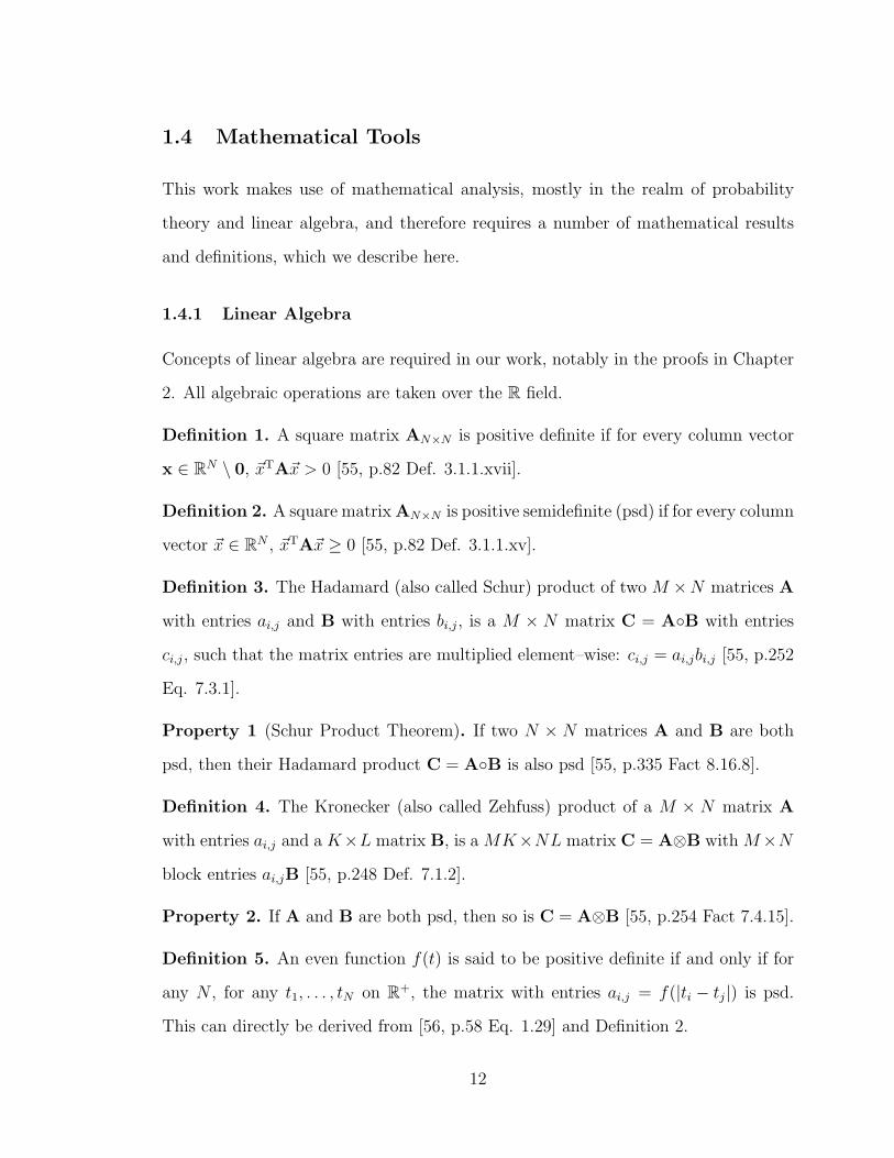
Definition 1. A square matrix AN×N is positive definite if for every column vector

x ∈ RN \ 0, xTAx > 0 [55, p.82 Def. 3.1.1.xvii].

Definition 2. A square matrix AN×N is positive semidefinite (psd) if for every column

vector x ∈ RN , xTAx ≥ 0 [55, p.82 Def. 3.1.1.xv].

Definition 3. The Hadamard (also called Schur) product of two M ×N matrices A

with entries ai,j and B with entries bi,j, is a M × N matrix C = A◦B with entries

ci,j, such that the matrix entries are multiplied element–wise: ci,j = ai,jbi,j [55, p.252

Eq. 7.3.1].

Property 1 (Schur Product Theorem). If two N × N matrices A and B are both

psd, then their Hadamard product C = A◦B is also psd [55, p.335 Fact 8.16.8].

Definition 4. The Kronecker (also called Zehfuss) product of a M × N matrix A

with entries ai,j and a K×L matrix B, is a MK×NL matrix C = A⊗B with M×N

block entries ai,jB [55, p.248 Def. 7.1.2].

Property 2. If A and B are both psd, then so is C = A⊗B [55, p.254 Fact 7.4.15].

Definition 5. An even function f(t) is said to be positive definite if and only if for

any N , for any t1, . . . , tN on R+, the matrix with entries ai,j = f(|ti − tj|) is psd.

This can directly be derived from [56, p.58 Eq. 1.29] and Definition 2.

12

Property 3 (Bochner’s Theorem). A continuous even function f(τ) is positive defi-

nite if and only if there exists a non–decreasing bounded function F (ω), ω ∈ R+ such

that [56, p.92 Eq. 2.53]

f(τ) =

∫ ∞

0

cosωτdF (ω). (1.1)

Property 4. Every covariance matrix is necessarily psd1 and symmetric [56, p.15

Eq. 0.36].

Property 5 (Polya’s Theorem). A bounded even function f(τ) with f(∞) = 0 that

is concave (up) on (0,∞) is necessarily positive definite [56, p.136]. (The converse is

not true.)

1.4.2 Gaussian Random Variables and Processes

We make extensive use of jointly Gaussian RVs and related concepts, which are well–

described in [58]; it is thus important to understand these well.

Definition 6. A Gaussian vector is one that can be obtained by a linear transfor-

mation on a vector of independent Gaussian RVs.

This leads to two basic properties that can be used to construct Gaussian vectors:

Property 6. A vector of iid standard Gaussian RVs is Gaussian.

Property 7. A linear transformation on a Gaussian vector is a Gaussian vector.

From these two statements, the following property follows:

Property 8. Any Gaussian vector is fully specified by its mean vector and covariance

matrix.

It is important to note that a vector of individually Gaussian RVs may not be a

Gaussian vector. Therefore:1Reference [57] says “positive definite”, but this is too restrictive; whereas [56] also says “positive

definite”, but this is a difference in nomenclature, and clearly psd is meant.

13

Definition 7. We call marginally Gaussian a vector of RVs that are individually

Gaussian.

A Gaussian vector is thus a particular case of a marginally Gaussian vector.

Definition 8. If a vector [Xi]Ni=1 is Gaussian, then we call

[eXi]Ni=1

a lognormal vector.

Similarly, if a vector [Xi]Ni=1 is marginally Gaussian, then we call

[eXi]Ni=1

a marginally

lognormal vector.

Definition 9. A random process (RP) X(t) is said to be Gaussian if, for any finite–

length vector of real values [ti]Ni=1, the vector [X(ti)]

Ni=1 is Gaussian. On the other

hand, a RP is merely marginally Gaussian if that vector is merely marginally Gaus-

sian.

Definition 10. If X(t) is a Gaussian RP, then we call eX(t) a lognormal RP. If X(t)

is a marginally Gaussian RP, then we call eX(t) a marginally lognormal RP.

Definition 11. A RP X(t) is said to be stationary if it is statistically invariant under

a shift, i.e., the vectors [X(ti)]Ni=1 and [X(ti + τ)]Ni=1 are statistically identical for any

constant τ .

Property 9. For any stationary RP X(t), its auto–correlation function (if it exists)

can be written E {X(t)X(t + τ)} = RX(τ) for any τ .

Together with Property 8, this leads to the following:

Property 10. A stationary Gaussian RP X(t) is fully specified statistically by its

mean µ and auto–correlation function RX(τ) = E {X(t)X(t + τ)}. A stationary log-

normal RP eX(t) can be fully described analogously by the mean and auto–correlation

function of X(t).

We are also interested in two–dimensional RPs, usually called random fields, where

stationarity is a somewhat more complex matter that needs to be defined more accu-

rately as follows:

14

Definition 12. A two–dimensional RP X(x, y) is said to be stationary [59] if it is

statistically invariant under translation, i.e., the vectors [X(xi, yi)]Ni=1 and

[X(xi + u, y + v)]Ni=1 are statistically identical for any u and v.

Property 11. For any stationary RP X(x, y), its auto–correlation function can be

written E {X(x, y)X(x + u, y + v)} = RX(u, v) for any u and v.

Together with Property 8, this leads to the following:

Property 12. A stationary Gaussian RP X(x, y) is fully specified statistically by

its mean µ and auto–correlation function E {X(x, y)X(x + u, y + v)} = RX(u, v). A

stationary lognormal RP eX(x,y) can be fully described analogously by the mean and

auto–correlation function of X(x, y).

Definition 13. A two–dimensional RP X(x, y) is said to be separable [60] if its auto–

correlation function may be written as E {X(x, y)X(z, w)} = Rx,X(x, z)Ry,X(y, w).

1.4.3 Convergence of Random Variables

Definition 14. A sequence X1, X2, . . . , XN of RVs with cumulative distribution

functions (cdfs) F1(x), F2(x), . . . , FN(x) converges in distribution [61] to an RV X

with cdf F (x) if

limN→∞

FN(x) = F (x), ∀x ∈ R. (1.2)

We write: XND−→ X as N → ∞.

It is important to note that convergence in distribution means the convergence of

the cdf at every point, but not necessarily of the probability density function (pdf),

even at any one point, as can be seen in the addition of discrete RVs.

Theorem 1 (Slutsky’s theorem [61]). Let XND−→ X as N → ∞ and YN

D−→ C a

constant as N → ∞. Then XNYND−→ XC as N → ∞.

15

Two points are of note regarding Slutsky’s theorem:

• The sequence {XN} need not be independent of the sequence {YN}.

• In general, this result does not hold if {YN} also converges to a non–constant

RV: the limit of the product of random sequences is not necessarily the product

of the limits.

Theorem 2 (The Central Limit Theorem [61]). Let Xi be a set of iid RVs with finite

variance VAR {X1}N∑i=1

Xi − E {X1}√NVAR {X1}

D−→ Z, (1.3)

where Z is a Gaussian RV with mean 0 and variance 1 [61].

Theorem 3 (The (Weak) Law of Large Numbers [61]). Let Xi be a set of iid RVs

with VAR {X1} < ∞N∑i=1

Xi

N

D−→ E {X1}. (1.4)

The CLT and the law of large numbers (LLN) are important tools in analysing the

sum of very many RV, and therefore relevant to the analysis of the sum interference

from many ISs. They are not, however, sufficient for our purpose, where we look at

correlated shadowing, and consequently at correlated interference components. We

therefore need to develop a more advanced limit theorem for our analysis, which we

do in Section 4.1.1.

1.4.4 Exchangeable Random Variables

The theory of exchangeable RVs was introduced by De Finetti [62–64]. Exchangeable

RVs are a central concept of this thesis, and can be seen as a generalisation of iid

RVs. Intuitively, a set of exchangeable RVs is simply one where the index assignment

is arbitrary, i.e., all permutations of the RVs have the same joint distribution. This

16

leads to a very wide set of applications, given that for any system where there are

elements of the same type (in our case, interferers) we see that the index assignment

is indeed arbitrary.

Definition 15. A permutation p(i), i = 1, . . . , N on a vector x = [xi]Ni=1 is any

bijective (one–to–one) mapping from the components of x onto itself.

Definition 16. A finite set of RVs {Xi}Ni=1 is said to be exchangeable if the vectors

[X1, X2, . . . , XN ] and[Xp(1), Xp(2), . . . , Xp(N)

]have the same joint distribution for any

permutation p(i) on the vector [1, 2, . . . , N ].

Theorem 4 (Hewitt–Savage Generalisation of de Finetti’s Theorem [65]). For any

exchangeable set {Xi}Ni=1, there exists a single RV Z such that all Xi’s are condition-

ally independent on Z. Equivalently, there exists a set of iid RVs {Yi}Ni=1 such that,

for all i, Xi can be written as a function of Z and Yi.

17

Chapter 2

Choosing a Good Shadowing Correlation Model

Correlation in wireless shadowing is a significant step in obtaining more realistic

channel propagation models. This chapter discusses in detail the existing literature

on shadowing correlation and the existing correlation models, focusing on evaluat-

ing which models are mathematically consistent, while also making comments on

their physical plausibility. The purpose of this chapter is to facilitate the choice and

implementation of correlation models in works that involve shadowing.

Recent work on various aspects of wireless communications has indicated a wide

gap between results obtained assuming independent shadowing paths and between

those that introduce correlation in shadowing propagation models [45, 46, 66–68].

Older works show that shadowing correlation significantly affects handover behaviour

[69–72], interference power [50, 53, 73–75] and consequently system performance [76–

78], and the performance of macrodiversity schemes [73,79–84]. Furthermore, shadow-

ing in dB has been measured [43, 79, 85–99] to have significant correlation in various

scenarios. Because of these two facts we believe that the general wireless commu-

nity is becoming convinced of the importance of modeling correlation in shadow-

ing [18, 41, 45–47, 67, 68, 75, 84, 100–106]. This is part of a more general trend sug-

gesting that most propagation models used in simulation (and analysis) work today

are sometimes too simplistic and may lead to misleading results [107]. Shadowing

18

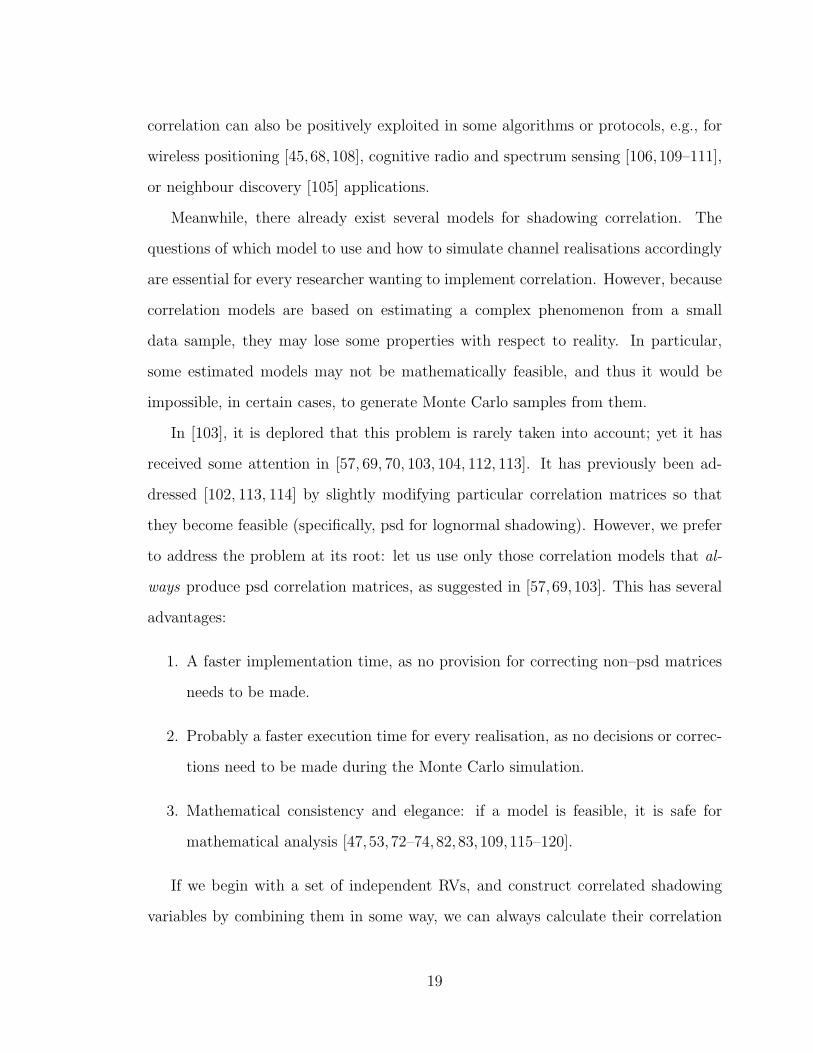
correlation can also be positively exploited in some algorithms or protocols, e.g., for

wireless positioning [45,68,108], cognitive radio and spectrum sensing [106,109–111],

or neighbour discovery [105] applications.

Meanwhile, there already exist several models for shadowing correlation. The

questions of which model to use and how to simulate channel realisations accordingly

are essential for every researcher wanting to implement correlation. However, because

correlation models are based on estimating a complex phenomenon from a small

data sample, they may lose some properties with respect to reality. In particular,

some estimated models may not be mathematically feasible, and thus it would be

impossible, in certain cases, to generate Monte Carlo samples from them.

In [103], it is deplored that this problem is rarely taken into account; yet it has

received some attention in [57, 69, 70, 103, 104, 112, 113]. It has previously been ad-

dressed [102, 113, 114] by slightly modifying particular correlation matrices so that

they become feasible (specifically, psd for lognormal shadowing). However, we prefer

to address the problem at its root: let us use only those correlation models that al-

ways produce psd correlation matrices, as suggested in [57,69,103]. This has several

advantages:

1. A faster implementation time, as no provision for correcting non–psd matrices

needs to be made.

2. Probably a faster execution time for every realisation, as no decisions or correc-

tions need to be made during the Monte Carlo simulation.

3. Mathematical consistency and elegance: if a model is feasible, it is safe for

mathematical analysis [47, 53,72–74,82,83,109,115–120].

If we begin with a set of independent RVs, and construct correlated shadowing

variables by combining them in some way, we can always calculate their correlation

19

structure. However, the inverse operation cannot always be performed: there does

not always exist a construction to obtain a desired correlation structure. Those that

cannot be constructed are termed not feasible.

2.1 Types of Correlation

In wireless communications, shadowing is a phenomenon that corresponds to a ran-

dom variability of the power gain over a (directed) propagation path. A transmitting

node radiates a radio signal toward a receiver node. The receiver may receive a desired

signal, or an interfering one. Shadowing represents the variability of the logarithm

of the received power around its expected value: we denote this quantity Si, with

VAR {Si} < ∞. The small–scale effect of fading has been removed in the spatial

dimension by averaging over a local region [103] of about 50 wavelengths [57, 118],

that is, approximately 8 – 34 meters for classic cellular channels [79,85–87,89,97,98].

Consider two directed paths,−−−→X1Y1 and

−−−→X2Y2, with shadowing values S1 and S2

respectively. Their correlation coefficient is defined as

ρ1,2 =E {S1S2}√

VAR {S1}VAR {S2}. (2.1)

In general, correlation may exist for any set of four points X1 = Y1, X2 = Y2. However,

we usually examine correlation under more specific scenarios.

2.1.1 Scenarios

Shadowing correlation can occur in various particular scenarios, specifically in peer–

to–peer links [40,44,45], in indoor, cross–floor, and indoor–outdoor links [87,90], and

in satellite–ground communications [91, 121–123]. It should be noted however that

most of the literature on correlation in shadowing is driven by cellular (usually urban)

20

Base Station Mobile Station

a)

Y1

Y2

X

S1

S2

b)

X

Y1

Y2

S1

S2

Figure 2.1: a) Shadowing auto–correlation for a mobile Y (t), b) Shadowing cross–correlation for a mobile X.

scenarios, where the base–station/mobile and uplink/downlink dualities apply. In cel-

lular communications, the distinction between auto–correlation and cross–correlation

applies [103]. Cross–sector correlation has also been considered [48].

An important consideration for satellite and indoor scenarios is that propagation

is usually considered in three, not just two, Cartesian dimensions. In this work we

analyse two–dimensional channel models only, although the analysis usually translates

easily to three dimensions.

2.1.2 Auto–Correlation

Also called serial correlation [124], this model considers a transmitting base–station

X, received by the same moving mobile Y at two moments in time, t1 and t2, and

at distinct locations Y1 = Y (t1) and Y2 = Y (t2). Alternatively, the signal may be

21

received by two distinct mobiles, Y1 and Y2, at the same moment in time. These sce-

narios may also be reversed to consider the uplink: either the same mobile transmits

to the same base station X at moments t1 and t2 at locations Y1 and Y2 respectively;

or the same base station X simultaneously receives from two distinct mobiles at loca-

tions Y1 and Y2. All these four cases can come under the category of auto–correlation

and are illustrated in Figure 2.1 a).

2.1.3 Cross–Correlation

This is the central object of our study. Cross–correlation, or site–to–site correlation

[124], considers two transmitting base stations, Y1 and Y2, that transmit to a common

mobile receiver X. Alternatively, cross–correlation can consider a mobile transmitter

X whose signal is picked up by two base stations, Y1 and Y2. These are illustrated in

Figure 2.1 b).

Now, observing the previous section on auto–correlation and the systematic nomen-

clature we gave to nodes (X a common node, and Y1 and Y2 nodes on two separate

links), we may abstract from the nature of these nodes and the link direction, and con-

clude that auto–correlation and cross–correlation are very similar in the mathematical

sense and can be studied in the same manner. Furthermore, we see in [104,125] how

an auto–correlation model can be used to model cross–correlation also. We therefore

assume that X is the common node to all paths, which we locate at the origin for

simplicity, and all links are between X and the points Yi.

2.1.4 Mathematical Synthesis of Auto– and Cross–Correlation

Auto– and cross–correlation models can be generically described as follows. Consider

N points Y1, . . . , YN located on a plane at positions r1, . . . rN with ri ∈ R2 \ {0}.

We assume, without loss of generality, that the common point X is located at the

origin, and thus ri =−−→XYi. Consider Si the logarithm of the power attenuation due

22

b

. . .

X

r1Y1

r2

Y2

rN

YN

S1

S2

SN

Figure 2.2: Generic geometry of shadowing auto– and cross–correlation.

to shadowing on each path ri (see Figure 2.2).1

We observe that both auto– and cross–correlation can be viewed under this same

framework, particularly given the common notation that we introduced for Figure

2.1. It is this common model that we intend to study. Then the shadowing model

can be entirely specified by the pair of functions (σ2s (r), h(r1, r2)).

2.1.5 Generalised Correlation

If we allow total freedom for the positions of the two paths, then the correlation model

becomes more complex; in fact, it becomes a function of up to eight free variables

(four free positions on a two dimensional plane).

We do not study this type of correlation for two reasons: first, because of its

increased complexity; and second, because the methods given in literature begin with

1At this moment, we need not commit to any particular shadowing distribution. We require onlythe condition that VAR {Si} < ∞.

23

an explicit construction of the shadowing realisations, and hence it is not necessary

to study their feasibility: they are always feasible. Contrast this with the correlation

models studied here. In Section 2.6.1, it is necessary to factorise a matrix, which is

not always possible, and thus the method is implicit and feasibility must be studied.

Such methods rely of generating shadowing maps or fields in some way. Three

algorithms for doing so are the Sum–of–Sinusoids (SoS) algorithm [40], the Network

Shadowing (NeSh) method [44–47], and the over–obstacle multiple–edge diffraction

model [39].

2.1.6 Time–Correlation

Time–correlation is different in that it only considers one path−−→XY , but looks at

the correlation between the shadowing at various moments in time. The shadowing

can thus be represented as a RP S(t) [71, 120]. The feasibility of the model is a

simple problem here, because the problem simply evolves in one dimension: time.

The correlation model is then specified by the auto–correlation function of S(t), and

the model is psd if and only if the auto–correlation function is psd. We are not aware

of any measurements of correlation in time only, and it is not evident if shadowing

changes significantly over a fixed path.

It should be understood that shadowing evolution in time should (like in space)

have fast fading removed through time–averaging of some duration.

2.1.7 Uplink–Downlink Correlation

Consider the path−−→XY , and then its return path

−−→Y X. By channel symmetry, one

might conclude that the shadowing experienced in both directions is identical, which

would correspond to a correlation coefficient of ρud = 1. In practice, measurements

indicate a high degree of correlation: ρud ≥ 0.66 [95]. From these measurements,

[126] assumed ρud = 0.7. Furthermore, [107] demonstrated asymmetry but positive

24

correlation in link connectivity, which can be interpreted as unequal but correlated

shadowing in each direction.

2.2 Positive Semidefiniteness of Correlation Models

From Property 4, for K to be a valid covariance matrix of S, it is a necessary (but

not always sufficient, as seen in Section 2.6) that K be psd (K is already symmetric

by construction).

Definition 17. We say that a shadowing model (σ2s (r), h(r1, r2)) is psd if ∀N, ∀[r1, . . . , rN ] ∈

(R2 \ {0})N

, the correlation matrix K is always psd.

2.2.1 Models with Variable Shadowing Variance

Theorem 5. If a model (1, h(r1, r2)) with constant log–variance 1 is psd, then

for any σ2s (r), the model (σ2

s (r), h(r1, r2)) is also psd. Conversely, if the model

(σ2s (r), h(r1, r2)) is psd and σ2

s (r) > 0 ∀r ∈ R2 \ {0}, then the model (1, h(r1, r2))

with constant log–variance 1 is psd.

Proof. Consider N shadowing paths ri ∈ R2\{0} and a shadowing model (σ2s (r), h(r1, r2))

where (1, h(r1, r2)) is a psd shadowing model. We call H the N×N matrix with entries

h(ri, rj), and s the column vector with entries σs(ri). Then the correlation matrix of

S can be written

K =(ssT)◦H. (2.2)

Now the matrix ssT is psd as can be seen from Definition 2: xT(ssT)x =

(xTs)2 ≥

0 ∀x ∈ RN . Also, since (1, h(r1, r2)) is psd, it follows that H is psd. Applying the

Schur product theorem, we find that K is always psd, which implies that the model

(σ2s (r), h(r1, r2)) is psd.

25

To prove the converse, we write

H =(zzT)◦K, (2.3)

where z is the column vector with entries σ−1s (ri), and the proof is analogous. Of

course, here the additional requirement that σs(r) = 0,∀r ∈ R2 \ {0} is required.

Thus in order to study the positive semidefiniteness of a shadowing model, it is

sufficient to study the correlation function h(r1, r2) in isolation, which simplifies the

problem. We therefore say that h is psd if (1, h) is psd.

2.2.2 Methods for Proving Positive Semidefiniteness

While we do not have a general criterion for proving that some given h is psd or not,

these few approaches nevertheless help us analyse most particular cases:

1. If there exists an explicit constructive algorithm for generating data according

to h, then h is necessarily psd, since the resulting covariance matrix is always

psd (see Property 4).

2. If there exists at least one choice of [r1, . . . , rN ] for which K is not psd, then h

is not psd. For this test, we need N ≥ 3, since every correlation matrix of size

2 is psd:

1 ρ

ρ 1

=

u v

v u

2

, u = 12

√1 + ρ+ 1

2

√1 − ρ, v = 1

2

√1 + ρ− 1

2

√1 − ρ. (2.4)

However, N = 3 may not be enough [113].

3. Several theorems can also be used to prove that some h is psd, as seen in the

next section.

26

2.2.3 One–Parameter and Separable Correlation

Proving that isotropic models (functions of d = ∥r1 − r2∥ only, with ri ∈ R2) are psd

is not trivial. Indeed, while for all psd models h(d), the function h(x) on R+ is positive

definite, the converse is not true, and tighter conditions are needed [56, p.361]. The

following two Theorems are examples of tests that can be applied to verify that h(d)

is psd:

Theorem 6. A one–parameter correlation model h(d) with d = ∥r1 − r2∥ with ri ∈

R2 is psd if 2 the integral

f(ω) =

∫ ∞

0

h(x)J0(ωx)xdx (2.5)

exists and is non–negative ∀ω ≥ 0. J0(x) is here the Bessel function of the first kind

of order 0. [56, p.357]

Theorem 7. A one–parameter correlation model h(d) with d = ∥r1 − r2∥ with ri ∈

R2 is psd if 2

1. the function h(x) with x ∈ R+ is positive definite and

2. the Fourier transform f(ω) of h(|x|) is non–increasing on ω ∈ (0,∞).

The converse is not true. [56, p.361]

Many other useful properties of isotropic correlation models are found in [56,

Chapter 22].

Theorem 8. A one–parameter correlation model h(θ) with θ = |∠r1 − ∠r2 + 2kπ|, k ∈

Z such that θ ∈ [0◦, 180◦] is psd if it may be written as

h(θ) =∞∑n=0

an cos (nθ), (2.6)

2These two theorems apply for shadowing on R2, and take a more restricted form on R3 [56].

27

for some non–negative and bounded sequence a0, a1, . . . with 0 <∑∞

n=0 an < ∞.

Proofs are given in [57,112].

Theorem 9. A one–parameter correlation model h(|x|) with |x| = |g(r1) − g(r2)| for

some function g : R2 \ {0} 7→ R is psd if it may be written as

h(x) =

∫ ∞

0

cos (2πxω)f(ω)dω (2.7)

for some non–negative and finite–area f(ω) on 0 < ω < ∞.

Proof. From Bochner’s Theorem, h(x) in (2.7) is a psd function. From Definition 5,

it follows that for any N the matrix HN×N with entries ρi,j = h(|ti − tj|), ti = g(ri)

is psd.

Theorem 10. If a correlation model h may be written as

h(r1, r2) = h1(r1, r2)h2(r1, r2) (2.8)

with h1 and h2 both psd, then h is also psd.

Proof. Let H, H1, and H2 be the N × N matrices with entries h(ri, rj), h1(ri, rj),

and h2(ri, rj) respectively. We may then write H = H1◦H2. Now since h1 and h2 are

psd, it follows that H1 and H2 are both psd. Applying the Schur product theorem,

we have that H is also psd, which implies that h is psd.

A similar argument was given in [57], but for positive definite instead of psd

matrices.

2.2.4 Incorporating Time and Uplink–Downlink Correlation

As seen in Section 2.1.6, shadowing may evolve in time in a correlated manner. Also,

as seen in Section 2.1.7, shadowing may be different on the same propagation path in

28

both directions, though these are usually highly correlated. We show that, given a pos-

itive definite temporal auto–correlation RS(τ) and a psd spatial correlation model h,

and assuming correlation separability between the spatial, time, and uplink–downlink

dimensions, the resulting combined correlation matrix is always psd. Combining

cross–correlation with temporal auto–correlation was described in [71].

Consider a common node X and N nodes Y1, . . . , YN . Let Si(t) be the shadowing

on path−−→XYi at time instant t with variance σ2

i = σ2s (ri), and Si(t) the shadowing on

the return path−−→YiX, with variance σ2

i = σ2s (ri).

Consider the spatial correlation function h such that ρi,j = h(ri, rj), i = j and

ρi,i = 1:

E {Si(t)Sj(t)} = σiσjρi,j ∀t,

E{Si(t)Sj(t)

}= σiσjρi,j ∀t.

(2.9)

We assume that the correlation between the two directions of the same path is con-

stant, as in [126]:

E{Si(t)Si(t)

}= σiσiρud ∀i ∀t. (2.10)

Consider also the normalised temporal auto–correlation function ζ(τ):

E {Si(t)Si(t + τ)}σ2i

=E{Si(t)Si(t + τ)

}σ2i

= ζ(τ) ∀i ∀t, (2.11)

where ζ(τ) is positive definite and ζ(0) = 1.

We further assume separability of cross–correlation and uplink–downlink correla-

tion, so that the correlation terms can be found as follows:

E {Si(t1)Sj(t2)}σiσj

=E{Si(t1)Sj(t2)

}σiσj

= ρi,jζ(t2 − t1),

E{Si(t1)Sj(t2)

}= σiσjρudρi,jζ(t2 − t1).

(2.12)

29

From this equation we see that separability implies that the uplink and downlink

cross–correlation models must be the same: h = h.

Consider M time instances t1, . . . , tM . Then the correlation matrix of S1(t1),

S1(t1), . . .,SN(t1), SN(t1), . . .,S1(tM), S1(tM), . . .,SN(tM), SN(tM) is

K2NM×2NM = [ζ(tj − ti)]M×M⊗

(ssT)◦[ρi,j]N×N⊗

1 ρud

ρud 1

, (2.13)

where s is the column vector with entries σ1, σ1, . . . , σN , σN .

Theorem 11. Given a psd correlation function h, uplink and downlink shadowing

variances σ2s (r), σ2

s (r), an uplink–downlink correlation coefficient −1 ≤ ρud ≤ 1, and

a normalised shadowing positive definite time auto–correlation function ζ(τ) with

ζ(0) = 1, and assuming the correlation is separable as in (2.12), we can conclude that

the composite correlation model is psd.

Proof. Consider (2.13). The matrix ssT is always psd, as seen in the proof of Theorem

5. The matrix [ζ(tj − ti)]M×M is psd because ζ(τ) is positive definite, and the matrix

[ρi,j]N×N is psd because h is psd. Finally, all 2 × 2 correlation matrices are psd, as

seen in (2.4). Both the Hadamard and the Kronecker products are psd if both their

factors are psd as seen in Properties 1 and 2. It follows that K is psd.

Simply speaking, one can incorporate (separable) directional and time correla-

tion without upsetting the positive semidefiniteness of the correlation model. Other

dimensions, notably frequency [106], may also be similarly incorporated.

One can note that the Kronecker product has been similarly used in [127] in a

multi–antenna context, and in [103] for correlation between shadowing, delay spread,

and angle spread, all under the assumptions of separability, which is natural when no

further information is available [103].

30

2.3 Estimating the Correlation Function fromMeasured Data

In order to better understand why estimated models may be psd or not, it is worth-

while to examine some aspects of how these models are constructed from measured

data.

2.3.1 Auto–Correlation as Mixed Time–Space Measurements

Auto–correlation is measured [43,85,86,88,92,96–99] by taking a single moving mobile

Y with velocity v in uniform rectilinear motion, measuring the power loss between Y

and a base station X, correcting for pathloss and small–scale fading, and considering

the shadowing S along the path−−→XY (or

−−→Y X) as a process of time S(t) (equivalently, of

space: S(dm), with dm = vt [128,129]). The underlying assumption is that shadowing

over a fixed link does not vary with time (or perhaps varies little or very slowly

compared to variation when in motion). More specifically, consider the shadowing

S(r, t) as would be experienced by a virtual mobile Y at time t and location r.

Now let the real mobile Y begin at location r0 at time t = 0 and move in uniform

rectilinear motion with velocity v. Thus its location at time t is r = r0 + tv. The

observed shadowing process at Y is thus S(t) = S(r0 + tv, t) or, equivalently, S(dm) =

S(r0 + dmv/v, dm/v). Clearly, the observed process varies in both time and space, and

assuming S(r, t) varies in t when r is fixed (see Section 2.1.6), these measurements

do not directly translate into a correlation model. For example, a different model

S(dm) might be extracted if the velocity v is changed. This is generally true for other

motion trajectories.

An additional issue about auto–correlation models is the level–crossing rate, which

is only properly defined for some models. This topic is addressed in [117,118,129–131],

and we do not explore it here further.

31

2.3.2 Cross–Correlation as Spatial–Only Correlation

Several field measurements have been performed [79, 85, 88, 89, 93, 94, 96–98] in order

to gather data about the true physical correlation model, which we call h. Field

measurements produce a set of data points, from which an estimate of the cross–

correlation function, which we call h, is obtained by fitting the data with plausible–

looking simple mathematical functions. It must be understood that h is always a psd

model, by its very mathematical definition. It was argued in [113] that a particular

conveniently psd model h may not reflect the true correlation accurately. This is true.

However, because h must be psd, it is likely that there exists some psd model h that

is close to h. Therefore, we argue that it is always best and possible to choose a psd

model h that is also close to h.

In general, h(r1, r2) is a function of four variables. However, estimating a four–

variable function accurately requires many more points than can realistically be ob-

tained from costly and cumbersome field measurements. Additionally, every point of

the function h is itself estimated as an expectation, and requires several data points.

Two consequences follow:

1. The measurement data is usually grouped by collapsing them from four variables

onto a single one.

2. On that one variable, the curve–fitting is still relatively crude [43,88,91,92,94,

99].

These two approximation steps further distance h from the h and may cause the

model h to be non–psd. Nevertheless, for practical reasons, it is simplest to measure

correlation along one dimension only [56, pp. 358–359].

32

r1

r2

θ

d

Y2

Y1X

R = 10ln 10

|ln r1r2|

Figure 2.3: A pair of auto– or cross–correlated paths, with the most relevant dimen-sional variables: d, θ, R.

2.3.3 Collapsing Correlation onto One Dimension

The measurements can be grouped along one variable in several ways. In such cases,

h is expressed as a function of a single free variable. The most common forms are:

1. Absolute distance (between Y1 and Y2) [43,85,86,88,91,92,96–99]: d = ∥r1 − r2∥.

2. Angle (not oriented) of arrival separation [57,85,88,93,94,96–98]: θ = |∠r1 − ∠r2| ∈

[0◦, 180◦].

3. Arrival distance ratio (in dB) [48,57,93,97]: R = |10 log10 r1/r2| = 10ln 10

|ln r1 − ln r2|.

These quantities are illustrated in Figure 2.3.

For correlation functions expressed in d, one may also estimate and fit the power

spectral density (which is the Fourier transform of the auto–correlation function in

differences of d) of the measured data to that of a particular model [88,92].

33

2.4 Specific Correlation Models and Their Positive Semidef-

initeness

We have made a wide (if not exhaustive) investigation of correlation models h used

in literature. All existing models imply jointly lognormal shadowing (which is by

no means a requirement of our analysis). Most models assume a constant shadowing

variance σ2s (r) = σ2

s , but not all [66,99]. As we have shown in Theorem 5, the positive

semidefiniteness of a shadowing model is separate from the shadowing spread function.

As such, we may safely study the existing correlation models, while looking forward

to more complex point–to–point shadowing spread models in the future.

The various existing models and their properties are summarised in Table 2.1. In

particular, we show which models are psd. While [103] stated that “most” models

are non–psd, we find that actually a slight majority of models are in fact psd.

The models are sorted according to the physical dimensions they take as param-

eters. A family tree of these models is illustrated in Figure 2.4. It should also be

understood that these models are not necessarily mutually exclusive when they are

expressed in different (d, R, θ) domains, since this implies a different reduction (inte-

gration) of the original four–dimensional model h onto one or two dimensions, possibly

representing different projections of the same h onto those dimensions.

2.4.1 Constant Model

The simplistic model that assigns ρi,j = ρ, i = j:

h(r1, r2) = ρ, (2.14)

with 0 < ρ < 1, is sometimes used [18, 41, 52, 68, 72–74, 81, 82, 89, 103, 110, 117, 119,

126, 132] (ρ = 0.5 [70, 84, 115, 116]) when more information is lacking. However,

34

constant

d

θ

θ, d; separable

θ, R; separable

θ, R; non–separable

θ, r1, r2; non–separable

increasing complexity

Figure 2.4: Shadowing correlation model families according to physical dimensionsdescribed in Figure 2.3. Other parameter combinations are possible but have notbeen encountered in literature.

[70] argued that this may be a too simplistic model, comparing simulations that

use constant versus non–constant models. On the other hand, we have shown [53]

that for a high number of highly–correlated lognormal–shadowed interferers, the total

interference power may be well approximated with the knowledge of the average

correlation coefficient only. (It is important to actually estimate this average. This

was not done in [70].)

The model is claimed psd for ρ = 0.5 in [103]. It does, in fact, give a psd H

for ρ ≥ −1/(N − 1) [52], and so the model is psd according to Definition 17 for

0 < ρ < 1 (and also ρ = 0, 1), but would be non–psd for −1 ≤ ρ < 0. It can be

simulated quickly [41,52] in the case of jointly lognormal correlated shadowing.

2.4.2 Absolute Distance–Only Models

All the auto–correlation models are expressed as a function of d (equivalently, of time

t, given a constant velocity v).

35

2.4.2.1 Exponential Model

The most common auto–correlation model is a decaying exponential of distance [10,

41, 43, 57, 69, 71, 86, 91, 96, 98–100, 103, 105, 106, 108, 109, 118, 122, 124, 125, 128, 130,

133–136]. This model is often attributed to Gudmundson in 1991 [43], though the

less–cited work by Marsan, Hess, and Gilbert in 1990 [86] also proposes this model,

and measurements by Graziano in 1978 [85, Figs. 5 and 7] suggest it. This model

has also been interpreted as a cross–correlation model [125]. It may be expressed as

h(d) = e−d/d0 , (2.15)

where d0 > 0 is the tunable parameter called the decorrelation distance (sometimes

defined for 50% correlation, rather than 1/e). Literature surveys have been made

[10,134] of the values that d0 might take in field measurements. While this model can

be understood as being based on a first–order auto–regressive (AR(1)), i.e., first–order

Markov, process [103], its positive semidefiniteness is not thereby evident, since, on a

non–linear trajectory, non–successive points may have different correlation coefficients

than simply those constructed by an AR(1) filter. The fact that e−x/d0 is a psd

function on R+ is a necessary but not sufficient condition [56, p.361] (the same applies

for any model depending on d). Nevertheless, this model is proved to be psd using

Theorem 6 in [56, p.362], and similarly in [57].

For equally–spaced ordered points Y1, . . . , YN on a straight line with separation

dsep, we have the correlation coefficients equal to ρi,j = ρ|i−j|, where ρ = e−dsep/d0 .

We then have a correlation matrix as in [137], which is necessarily psd, because the

model (2.15) is psd.

36

2.4.2.2 More Complex Models

The exponential model has inspired some more complex models, which may be inter-

preted as auto– or cross–correlation models.

In [88, 92, 138], a sum of two independent exponential processes is used, which

leads to the following correlation model:

h(d) = ae−d/d1 + (1 − a)e−d/d2 , (2.16)

where 0 ≤ a ≤ 1, 0 < d1, 0 < d2 are tunable parameters. This model is always psd.

Proof. Applying (2.16) in (2.5), we may separate the resulting integral by linearity

into two integrals, both of which are non–negative as seen for the model (2.15), and

weighed by the non–negative coefficients a and 1 − a. The resulting integral (2.5)

for this model is thus non–negative. It follows from Theorem 6 that this model is

psd.

In [117,129] (and implicitly in [131]), a Gaussian correlation model is used:

h(d) = e−(d/d)2, (2.17)

where d > 0 is the tunable parameter. This model is proved to be psd using Theorem

6 in [56, p.364].

In [131], a convolution of an exponential and a Gaussian function is proposed:

h(d) = Ke−|d|/d0∗e−(d/d)2

= K

∫ ∞

−∞e−|d−t|/d0−t2/d2dt, (2.18)

where d0 > 0, d > 0 are the tunable parameters, and K = exp(−d2/4d20

)/√πd. This

model is psd.

37

Proof. The Fourier transform of (2.18) with x = d is

f(ω) = K2/d0

ω2 + d−20

d√πe−

14(dω)

2

,

which meets the conditions of Theorem 7.

In [42], a model is proposed that can be written:

h(d) = e−(d/d0)ν

, (2.19)

with d0 > 0, ν > 0 tunable parameters. The positive semidefiniteness of this model

is dependent on ν: for 0 < ν ≤ 2, it is proved to be psd with the aid of Theorem

7 in [56, p.364]. This of course includes the models (2.15) and (2.17), as well as

the choice of ν = 0.9682 in [42]. For ν > 2 however, the model is in non–psd [56,

p.137]. As a counterexample, consider three aligned points with equal consecutive

spacings of 0.2d0, for which we find that the correlation matrix is not psd for ν =

2.1, 2.2, 2.5, 3, 5, 50.

2.4.3 Angle–Only Models

Some of the first shadowing correlation measurements along θ were reported in [79,

85], but no analytical model was extracted. A similar measurement campaign [97]

reported much lower angular correlation, suggesting the need for a more complex

model. However, it has been argued [103] that θ is the most significant parameter in

cross–correlation, which justifies using these models as a first approximation.

In [112,133], and later in [76,139], a cosine model was proposed:

h(θ) = A cos θ + B, (2.20)

38

with two tunable parameters A ≥ 0, B ≥ 0, A + B ≤ 1. The model was used

and assumed psd in [103]. Typical parameter choices have been A = 0.3, B = 0.5

[78,80,82,118] and A = 0.3, B = 0.699(9) [76,139].

The model was proved to be psd in [57, 69, 112] using Theorem 8, by setting

a0 = A, a1 = B and all other an = 0.

In [94], a piecewise–linear model was proposed:

h(θ) =

0.78 − 7θ/1250◦ 0◦ ≤ θ < 15◦,

0.48 − 7θ/1250◦ 15◦ ≤ θ < 60◦,

0 60◦ ≤ θ ≤ 180◦.

(2.21)

It was shown in [113] that this model is non–psd. Here is an example: N = 7 with

∠ri = 0, 5, . . . , 30◦.

In [93, Table 1], a lookup table for intervals of θ, effectively a piecewise–constant

model was given:

h(θ) =

0.6 0◦ ≤ θ < 30◦,

0.25 30◦ < θ < 60◦,

α ≥ 0.2 θ ≥ 90◦.

(2.22)

This model is undefined for θ ∈ {30◦} ∪ [60◦, 90◦]. We understand that a value for

α may be chosen on [0.2, 0.25]. Regardless of the missing information, the model is

non–psd, as shown in this example: N = 11 with ∠ri = 0, 4, . . . , 40◦.

A triangular model in θ was proposed in [48]:

h(θ) =

a− (a− b)θ/θ0 θ ≤ θ0,

b θ > θ0,

(2.23)

with 0 ≤ b < a ≤ 1 and 0◦ < θ0 ≤ 180◦ three tunable parameters. In [48], the model

39

a = 0.8, b = 0.4, θ0 = 60◦ was used to fit the measurements in [85]. The same choice

of parameters was proposed for cross–correlation modeling for the 802.16m standard

[135]. Also, a = 0.8, b = 0, θ0 = 60◦ was proposed to fit the measurements in [94],

previously fitted with (2.21). In [88], the same model with a = 0.9, b = 0, θ0 = 180◦

was used. This model is always psd for any choice of parameters.

Proof. Consider

a0 = b + (a− b)θ02π

, an = 2(a− b)1 − cos θ0n

πθ0n2.

Using Theorem 8 yields (2.23).

A decaying exponential angle model has also been proposed [57,67,101,140]:

h(θ) = e−αθ, (2.24)

with α > 0 a tunable parameter. This model can be seen as inspired from the

exponential d model (2.15), which it approximates for small θ. This model is psd [57].

Proof. Consider

a0 =1 − e−απ

απ, an =

2

π

α

n2 + α2

(1 − e−απ(−1)n

).

Using Theorem 8 yields (2.24).

2.4.4 Separable Models

Separable models are easily constructed from the multiplication of one–dimensional

models. Theorem 10 shows that if the component one–dimensional models are psd,

so is the composite separable model.

40

2.4.4.1 Angle–Distance Ratio

Separable θ–R models may always be written as

h(θ, R) = hΘ(θ)hR(R). (2.25)

The use of the θ and R dimensions for shadowing correlation models has been argued

in [48,57,97,98,103,118], though separability may be a simplistic assumption [57].

In [48], the model “1.0/0.0 RX” is given as

hΘ(θ) =

1 − θ/75◦ θ ≤ 60◦,

0 θ ≤ 60◦,

(2.26)

and

hR(R) = max (0, 1 −R/R0), (2.27)

with R0 > 0, with R0 usually in [6 dB, 20 dB]. This model is not psd, as shown in the

following example: let N = 7 and all ri equal, and let ri = 0, 15, . . . , 90◦.

The problem with the preceding model is its discontinuity at θ = 60◦. This is

simple to resolve: if we use the general form (2.23) as hΘ(θ) and (2.27) as hR(R), we

have a very flexible model that is always psd.

Proof. hR(R) is shown to be psd by choosing

f(ω) =2 sin2 (πR0ω)

π2R0ω2

with g(r) = 10ln 10

ln ∥r∥ in Theorem 9. Equivalently, we may use Polya’s Theorem, as

in [57].

The model (2.23) was already shown to be psd.

Now h is expressed as a product of two psd models, and it follows from Theorem

41

10 that h(θ, R) is psd.

2.4.4.2 Angle–Absolute Distance

In [104], a separable model depending on d and θ is used, and can be rewritten:

hd(d) = e−d/d0 ,

hΘ(θ) =

1 θ ≤ 90◦,

0 θ > 90◦,

h(d, θ) = hd(d)hΘ(θ).

(2.28)

(There is a mistype in the original equation [104, eq. 18]: the term σ2ψp

should be

removed, as confirmed in a private communication with D. Kaltakis).

The authors say that this model is psd; however, this claim is not substantiated,

though we understand that their simulations always gave psd correlation matrices.

We already recognise the model hd(d) from (2.15), which we know to be psd. However,

it is simple to show that hΘ is non–psd, therefore the product of the two might not

be psd either. In fact, the following counterexample shows it is not psd: N = 14 with

ri = d0, ∠ri = 0, 180/7, . . . , 2340/7◦.

The authors of [104] claim that this model is psd, based on their simulations. This

is to be expected: because the model can be approximated by (2.15) for ri ≫ d0, as

might be the case in the cellular context, it can often appear psd in simulations.

However, strictly speaking, it is non–psd, and our example shows that it can fail,

particularly in cases of small ri.

42

In [141], the same author proposes

hd(d) = e−d/d0 ,

hΘ(θ) = max (0, cos (θ))

h(d, θ) = hd(d)hΘ(θ).

(2.29)

Again, while the model appears psd [141], in fact it is not, as attested by the fol-

lowing counterexample: N = 8 with ri = 0.4d0, ∠ri = 0, 45, . . . , 325◦. However, this

is a case with very small ri. In practice, for ri ≫ d0, this model is well–approximated

by

h(d, θ) = e−d/d0 cos (θ), (2.30)

which is psd.

Proof. Model (2.30) is the product of models (2.15) and (2.20) with A = 1, B = 0,

both of which were shown to be psd. Then, by Theorem 10, (2.30) is psd.

2.4.5 More Elaborate (Non–Separable) Models

It has been suggested [57] that separable models might not be sufficient to accurately

model shadowing correlation.

Saunders’ model [124] has been used in [70,102,103,113,142] (but watch for various

transcription errors):

h1 = 10−0.05R, h2 =

1 θ < θT,

(θT/θ)γ θ ≥ θT,

θT = 2 arcsind0

2 min {r1, r2}, h(θ, r1, r2) = h1h2,

(2.31)

where d0 is the same correlation distance as measured for model (2.15), and γ > 0 is

43

the other tunable parameter (a typical value is γ = 0.3). The model is not separable

in θ and R because θT depends on r1 and r2. This model is non–psd, as seen in

[103,104,113] and as is apparent from this example: N = 3 with ri = r ≥ d0/√

2 and

∠ri = 0, θT, 2θT.

Also, we see that this model is undefined for ri < d0/2, since the domain of arcsin

is [−1, 1]. To rectify this problem, Saunders’ model has been modified [66] (also [136],

but note some transcription errors) by augmenting its domain:

h(θ, r1, r2) =

as in (2.31) r1, r2 ≥ d0/2,√d0/2 max {r1, r2} otherwise.

(2.32)

Notice however that if more than one ri is less than d0/2, we again have h > 1, which

is not a valid correlation value.

Also, extending the model’s domain cannot make it psd: the same counterexam-

ples used to show that (2.31) is non–psd can be used to show that (2.32) is non–psd.

Another model was given in [93, Table 2] and used in [103]. It is piecewise constant

on rectangles in the θ–R domain:

h(θ,R) =

R < 2 2 < R < 4 R ≥ 4

0.8 0.6 0.4 θ < 30◦,

0.5 0.4 0.2 30◦ < θ < 60◦,

0.4 0.4 0.2 60◦ < θ < 90◦,

0.2 0.2 0.2 θ ≥ 90◦.

(2.33)

The entries of this table cannot be obtained from an outer product, and thus the

model is non–separable. The model is non–psd, as observed in [103, 104, 113]; for

example: N = 6 with ri = r ∀i and ∠ri = 0, 7, 14, 21, 28, 35◦.

44

Another model is given in [83]:

hΘ(θ) as in (2.21),

hR(R) = max (0, (1 −R/R0)α)

h(θ,R) = hR(R)(hΘ(θ) + a) + b,

(2.34)

with a > 0, b > 0, a + b ≤ 0.22, α ≥ 0 and R0 > 0. When b = 0, this model is

not quite separable. It is not psd, as seen from the same counterexample as used for

model (2.21), with a = b = 0 and ri = r ∀i.

Finally, the model “1.0/0.4 RX” in [48] takes the form:

h(θ, R) =

max

(0, 1 − R

R0

)(0.6 − θ

150◦

)+ 0.4 θ ≤ 60◦,

0.4 θ > 60◦,

(2.35)

where R0 is chosen between 6 and 20 dB. This model is not psd, as attested by the

following example: with N = 4, regardless of the value of R0, choose ri all equal, and

∠ri = 0, 30, 60, 90◦.

2.5 Some Thoughts on Physical Realism

While this chapter focuses on the mathematical feasibility of correlation models, we

would like to give a few thoughts about physical realism as well: can the correlation

model h be considered realistic, based on what we know about wireless propaga-

tion? Does it make sense intuitively? It is important to keep in mind that, while

mathematical feasibility is an objective criterion, physical plausibility is relative to

the understanding of wireless shadowing, and therefore the criteria presented in this

section are merely tentative. We hope that these initial ideas will encourage thought

and discussion on what a shadowing correlation model should realistically look like.

45

Table 2.1: Summary of existing shadowing correlation models and their properties.

Model Name Equation Tunable Parame-ters

References Dimensions psd Physical Proper-tiesb Violated

Constant (2.14) 0 < ρ < 1 many none Yes 1, 5, 7

Exp(d) (2.15) d0 > 0 [43,86], ... d Yes 7

Exp+Exp(d) (2.16) 0 ≤ a ≤ 1, 0 <d1, 0 < d2

[88, 92,138] d Yes 7

Gaussian(d) (2.17) d > 0 [129] d Yes 7

Exp∗Gaussian(d) (2.18) d0 > 0, d > 0 [131] d Yes 7

Exp(dν) (2.19) d0 > 0, 0 < ν ≤ 2 [42] d Yes 7

d0 > 0, ν > 2 No 7

Cos(θ) (2.20) A ≥ 0, B ≥ 0, A +B ≤ 1

[76,112,133,139] θ Yes (1)c , (2)c , 4, (5)c

Piecewise(θ) (2.21) none [94] θ No 1, 6

Stepwise(θ) (2.22) none [93, Table 1] θ No 1, 5, 6

Triangular(θ) (2.23) 0 ≤ b < a ≤ 1, 0◦ <θ0 < 180◦

[48] θ Yes (1)c , (2)c , (5)c

Exp(θ) (2.24) α > 0 [57,67,101,140] θ Yes 2, (5)c

“1.0/0.0 RX” (2.25),(2.26),(2.27)

R0 > 0 [48] θ,R No 6

Triangular(θ) ×Triangular(R)

(2.25),(2.23),(2.27)

0 ≤ b < a ≤ 1,0◦ < θ0 < 180◦,R0 > 0

modified [48] θ,R Yes (1)c , (5)c

b = 0, a = 1 Yes none

Exp(d)×(θ ≤ 90◦) (2.28) d0 > 0 [104] d, θ No 6

Exp(d)× cos+(θ) (2.29) d0 > 0 [141] d, θ No none

Exp(d)× cos (θ) (2.30) d0 > 0 modified [141] d, θ Yes 4

Saunders’ (2.31) d0 > 0, γ > 0 [124,143] (θ, r1, r2)a ,ri > d0/2

No 2, (5)c

Modified Saun-ders’

(2.32) d0 > 0, γ > 0 [66] (θ, r1, r2)a ,r2, . . . , rN >d0/2

No 2, 3, (5)c , 6

Stepwise(θ,R) (2.33) none [93, Table 2] (θ,R)a No 1, 5, 6

Piecewise(θ)–Triangularα(R)

(2.34) R0 > 0, α ≥ 0, a >0, b > 0, a+b ≤ 0.22

[83] (θ,R)a No (1)c , (5)c , 6

“1.0/0.4 RX” (2.35) R0 > 0 [48] (θ,R)a No 5, 6

aNon–separablebAs described in Section 2.5cPhysical property met only for some parameter choices

Nevertheless, these initial criteria can give a first approximation in choosing a good

correlation model.

Proposition 1. Shadowing is a large–scale phenomenon, averaged over small dis-

placements in space (and time), and should not by nature vary quickly in these

46

dimensions [43,57,103,118].

Proposition 2. As argued in [10, 48, 70, 79, 97, 115, 116, 124, 142, 143], correlation

in shadowing may be explained by a partial overlap of the large–scale propagation

medium, as seen in Figure 2.5. The non–overlapping propagation areas are considered

independent. When a propagation front passes through successive areas, the gains

are multiplicative, and thus add in the logarithmic domain. We may then write:

Let W,W1,W2 be independent RVs with zero mean and variances w2, w21, w

22 re-

spectively. We have

S1 = W + W1,

S2 = W + W2.(2.36)

It follows that

VAR {S1} = w2 + w21 = σ2

s (r1),

VAR {S2} = w2 + w22 = σ2

s (r2),

E {S1S2} = w2,

(2.37)

and therefore

h(r1, r2) =w2√

(w2 + w21)(w

2 + w22). (2.38)

This applies to any pair of shadowing terms.

This interpretation leads us to formulate the following criteria:

1. h(ri, rj) ≈ 1 for ri ≈ rj.

2. h(ri, rj) ≪ 1 for ∥ri − rj∥ ≫ 0.

3. h should be a non–increasing function in θ [57,85,93,103], R [93] and d.

4. h should be non–negative, according to (2.37). However, this is contradicted

by some measurement campaigns [43,85,87,90,94,96–99], which reported some

significantly negative estimated correlation coefficients in some cases. It would

47

b

X

Y1

Y2

W1

W2

W

Figure 2.5: Physical argument of common propagation area for correlation in shad-owing.

be interesting to study whether these observations are statistically significant.

Also, we suspect that negative correlations in measurements may appear in a

particular obstacle scenario. However, averaged over very many obstacle reali-

sations, the correlations are perhaps less likely to be negative.

5. h should be small for large θ, and approach zero for θ ≈ 180◦ and r1, r2 large,

as the propagation regions are then essentially non–overlapping.

6. Continuity: a small change in ri should result in small changes in h(ri, rj), at

least when ri is large.

7. Correlation should not depend on d only, as the distance between r1 and r2 tells

us little about the overlap between the corresponding propagation areas.

Furthermore, it was argued [48, 57, 97, 98, 103, 118] that cross–correlation should de-

pend on θ and R.

We have checked each model against these physical constraints, and summarised

the results (without proof) in Table 2.1. The only model that is both psd and fulfills

all these physical criteria is the one we proposed based on [48], given by (2.23), (2.25),

and (2.27), with a = 1, b = 0.

48

2.6 Feasibility According to Marginal Distribution

Until now, we have only verified whether a given model h gives psd covariance matrices

K. This is a necessary but not always sufficient condition to ensure that a random

vector S can be constructed with covariance K. To further study feasibility, it is

necessary to look at the marginal distribution of Si.

2.6.1 Jointly Lognormal Shadowing

In the most common case of lognormal shadowing (i.e., each Si being Gaussian), a

natural and effective way to model shadowing paths jointly is by making S1, . . . , SN

jointly Gaussian. We then say that shadowing is jointly lognormal. In this case, every

symmetric psd correlation matrix is feasible, by the following explicit construction:

We begin by solving for CN×N in

K = CCT. (2.39)

In general, there are many solutions to this equation if and only if K is psd. Then, we

generate an independent column vector of standard Gaussian RVs Z = [Z1, . . . , ZN ],

and obtain the shadowing terms with

S = CZ. (2.40)

This is a constructive proof that, for lognormal shadowing, feasibility is equivalent

to positive semidefiniteness.

2.6.2 Non–Lognormal Shadowing

While lognormal is a well–established and by far the most common model for the

marginal distribution of shadowing, it is not the only one available. Other models have

49

been proposed, either from physical plausibility arguments, or for easier mathematical

tractability. The two other models that we have encountered for the distribution of

eλSi are truncated lognormal [10,144] and Gamma [145–147]. See [10, Section V-B-4]

for a survey of shadowing distribution measurements.

We have seen in Section 2.1.4 that the condition of finite variance of Si is required

for an adequate definition of correlation. For the truncated lognormal model, which

corresponds to a truncated Gaussian Si, it is easy to see that truncation reduces the

variance, hence it is finite. For Gamma shadowing, it is easy to verify that all the

moments of the logarithm of a Gamma RV are finite, since they can be expressed as

the integral 4.352.1 in [148].

It is, however, not evident that the vector S can be generated according to non–

Gaussian marginal distributions and a given psd correlation matrix K. One construc-

tive method for obtaining such jointly distributed vectors is NORTA (Normal–to–

Anything), described in [149]. This method requires some more stringent conditions

on the marginal distributions to be feasible. These conditions might merit further

study should non–lognormal shadowing models gain in popularity.

2.7 Consequences for Working with Correlated Shadowing

We propose the criteria developed in this chapter as a basis for evaluating, designing,

and correcting existing future correlation models. There is naturally more to be said,

both on testing more complex models for being psd and on the physical plausibility

of those models.

50

2.7.1 For Those Wanting to Incorporate Shadowing Correlation

For lognormal shadowing, only certain models that have the psd property (see Ta-

ble 2.1) guarantee to always give feasible joint shadowing distributions. For non–

lognormal shadowing, some additional conditions might be required.

Based on both mathematical feasibility and physical arguments, we conclude that

a subset of the family of models given by (3.5) and inspired by [48] is the best existing

candidate for modeling correlation in shadowing. With two tunable parameters, θ0

and R0, it may be tuned to approximate many other correlation models that might

have less desirable properties.

2.7.2 For Those Using a Model that Is Not Feasible

Models that are not psd may still be used in particular application scenarios. For

example, all models give psd correlation matrices for N = 2. Also, we have argued

that a correlation model that corresponds exactly to reality must per force be psd.

It follows that for any model that approximates reality well (whether from extensive

measurement campaigns or from theoretical arguments), there exists a model that is

close to it (according to some reasonable metric) while also being psd. For example,

the authors in [48] fit the psd model (2.23) to the data of [85] to replace the non–psd

model (2.21).

Our suggestion is to take non–psd models and correct them slightly to make them

psd, as we have done for (2.29).

2.7.3 For Those Designing New Correlation Models

We suggest that all new correlation models be designed as psd for the reasons de-

scribed at the beginning of this chapter. Theorem 10 can be used to construct more

detailed separable models.

51

2.7.4 For Those Studying Large Interference Problems

Finally, a very important specific application of shadowing correlation is the study of

the aggregate interference from a large number of devices. The resulting interference

distribution differs greatly whether one considers shadowing that is independent, or

one that is significantly correlated; this effect becomes more significant as the number

of interferers increases. It is this interference distribution that we examine in the rest

of the thesis.

52

Chapter 3

Problem Statement

In this chapter, we specify the quantities and parameters that describe our physical

interference problem. Many quantities are random, and these should all be considered

fully independent unless specified otherwise. The problem is specified by a description

of the wireless channel, of the locations of the ISs and their transmit characteristics,

and of the manner in which individual interference signals combine.

3.1 Interferer Layout

Since we consider large numbers of wireless (often mobile) ISs, it is natural to position

them randomly according to some spatial distribution, rather than give all their

positions explicitly [2, 3].

We always assume that the RX is located at the origin of the plane, and the

positions of the ISs are vectors in 2 dimensions: ri ∈ R2 \ {0}, with ri = ∥ri∥.

3.1.1 Poisson Field

A mathematical model for IS positions that is very simple conceptually is a two–

dimensional homogeneous Poisson point process (PPP) [4, 25, 150], sometimes called

a Poisson field. It is characterised simply by a scalar density λP. It can be simply

53

defined by stating that for any Borel region A of finite Lebesgue measure (area)

|A|, the number of ISs inside A follows a Poisson distribution with mean λP|A|.

Furthermore, for any set of such disjoint areas, the numbers of points lying inside

those areas are independent [150].

Equivalently, we may construct such a process by considering a circular region of

radius rmax centered at the origin, and generating N iid uniformly–distributed points

ri on the disc, where N is a Poisson RV with mean πr2maxλP, then taking rmax → ∞.

For simulation purposes, it is necessary to limit rmax to a large finite value.

In [150], a finite area of ISs is considered, modeled as a Bernoulli Point Process,

which is somewhat more general, but still very restrictive. These models are the

starting point for our thinking about layouts. Still, we eschew the above two models

in favour of a much more general layout described by a weighted spatial distribution.

3.1.2 Weighed Spatial Distribution

A much more generalised approach [32] is to sample the positions ri from a 2–

dimensional pdf g(r), i.e., for any Borel set A in R2, we have P (ri ∈ A) =∫A g(r)dr.

It is also convenient to define Ag the entire area where g is non–zero, and rmin, rmax,

the tightest bounds such that g(r) = 0 for r outside [rmin, rmax]. The interfering net-

work is then composed of N ISs with positions chosen iid from g(r). In this thesis, we

consider N to be a non–random quantity. However, in Section 6.2.1 we describe how

to modify our work to incorporate a random N , e.g., from a Poisson distribution.

This is a quite general formulation of the problem and can include many con-

ceivable scenarios. Still, it cannot model particular behaviours, such as thinning,

clustering, or other phenomena between the ISs that require dependence among the

IS positions [151, 152]. We do not consider such effects in this thesis, but show in

Chapter 6.2.2 how they may be incorporated.

54

3.1.3 Cluster Layouts

As a subset of the generalised spatial distribution g(r) just given, we take special

interest in those that exhibit what we call a cluster geometry. We do not give an

exact definition of a cluster layout. Rather, as a rule of thumb, we suggest that a

cluster of interferers is one where (almost) all the ISs are seen at a fairly narrow

angle from the RX (not much more than a 60◦ spread), and that the cluster of ISs

has roughly circular symmetry, as a consequence of which the spread of the distances

between the RX and the ISs is not too significant (not much more than 4 to 1 for

farthest to nearest).

A cluster layout generally applies in the case where the RX and the ISs do not

belong to the same network, simply because of the nature of such a geometry. The

cluster layout is of interest to us because it is only in this case that we find a simple

mostly analytical solution.

3.1.4 Layout Examples

In this thesis, we use four specific layouts, which we illustrate in Figure 3.1:

A A uniform distribution over a square region away from the RX. This is an example

of a cluster layout.

B A circular Gaussian distribution truncated at four standard deviations over a cir-

cular region away from the RX. This is another cluster layout.

C An annular region centred around the RX. There is a relatively small exclusion

region around the RX to prevent problems with ISs arbitrarily close to the RX.

This type of layout is usually assumed (with possibly the outer radius going to

infinity, and possibly the inner radius zero) in the literature described in 1.2.2.

D A very thin annular region centred around the RX. This is not really a likely

55

A : Square Cluster

g(x, y) =

19· 10−4 100 < x < 400,

100 < y < 400

0 otherwise

100 300

RX

B : Gaussian Cluster

g(r) =

e−∥r−rc∥2

2252/8

(1−e−4)2252π/8∥r − r0∥ < 225

0 otherwise

where rc = (275, 0)

50 225

RX

C : Surrounding Ring

g(r) =

{(247500π)−1 50 < r < 500

0 otherwise

50500

RX

D : Surrounding Thin Ring

g(r) =

{(99.99π)−1 499.9 < r < 500

0 otherwise

499.9

500

RX

Figure 3.1: Interferer layouts used in this thesis. Distances are in meters.

56

real world scenario. Instead, we only use it to separate the effect of shadowing

from pathloss in order to better understand the effects of each. Indeed, in this

layout, r, and thus the pathloss, is almost constant.

3.2 Channel Models

In this section, we define the propagation channel between two points, as well as the

correlation between two paths with one common point. We are interested exclusively

in large–scale outdoor propagation scenarios. Also, we consider a single frequency

channel at a single moment; there is thus no modeling across frequency or time (we

discuss this issue briefly in Section 6.2.5). We consider pathloss, shadowing, and

shadowing correlation, but not small–scale fading. In Section 6.2.3, we discuss how

small–scale fading can be incorporated into our results without much effort.

Various components come together to make up the channel model between a

transmitter and a receiver. These are modeled as RVs, whose statistics are known

either through estimation based on empirical measurements in the field, or through

physical arguments.

3.2.1 Average Pathloss

The average pathloss is a deterministic function of distance, which we denote p(r).

Pathloss is often [4,37,57] modeled as power–law: p(r) = r−β for 2 ≤ β ≤ 6. However,

to allow for the incorporation of both very near and very far–away interferers, more

flexibility in the model is useful.

To this end, we use a model that behaves similarly to free–space (β = 2) before

the Fresnel breakpoint and according to a two–ray model (β = 4) for larger distances

57

[153]. The model is based on [154] and is given by

p(r) = r−2(1 + r/150)−2. (3.1)

The distances are in meters, and we see the breakpoint around 150 meters, with the

added elegance of a smooth transition. This model is taken as a realistic example

only and does not restrict the scope of our work.

3.2.2 Lognormal Shadowing

The lognormal distribution is a well established [10, 71, 87, 124, 128] model for large–

scale wireless fading, i.e., shadowing. The shadowing gain (in dB) between an IS i

and the RX is then given by a Gaussian RV Si with mean 0, and variance σ2s (r) a

function of distance. The power on that path is then scaled by a factor of eλSi , with

λ = 0.1 ln 10.

While shadowing is often found to have approximately constant spread σs over

distance, this may not be the case for very short distances. Indeed we may use the

following model, taken from [66]

σs(r) = 10(1 − exp (−3r/200)) dB, (3.2)

where the distances are in meters. We see that the shadowing spread stays within

5% of 10 dB for distances above 200 meters. Again, this is just a useful example of a

model to illustrate our work.

3.2.3 Spatially–Correlated Jointly Lognormal Shadowing

Of great importance to this work is the joint distribution of the shadowing paths.

While little is known about the exact nature of this distribution, the most common

58

(in fact, perhaps the only) approach is to consider the shadowing paths as jointly

lognormal (when conditioned on position). This approach could be said to be the

most natural to formulate and to use, and goes as follows:

We construct a vector S = [Si]Ni=1 that is (jointly) Gaussian when conditioned on

r1, . . . , rN . The vector is fully statistically described by the quantities

E {Si} = 0,

E{S2i |ri}

= σ2s (ri),

E {SiSj|ri, rj} = σs(ri)σs(rj)h(ri, rj),

(3.3)

where h is the shadowing correlation model, with −1 ≤ h ≤ 1 and h(ri, rj) = h(rj, ri).

Then, the correlation matrix of S conditioned on r1, . . . , rN is given by

K =

σ21 σ1σ2ρ1,2 · · · σ1σNρ1,N

σ1σ2ρ1,2 σ22 · · · σ2σNρ2,N

......

. . ....

σ1σNρ1,N σ2σNρ2,N · · · σ2N

. (3.4)

Shadowing correlation models are discussed in Chapter 2, where we conclude with

the choice of the following model, which is inspired by [48]:

h(ri, rj) = max {1 − θ/θ0, 0} · max {1 −R/R0, 0}, (3.5)

where θ and R are defined in Section 2.3.3, and the model has two tunable parameters:

0◦ < θ0 ≤ 180◦ and R0 > 0. Note that the model is separable in θ and R.

We choose this model among many others for the following reasons:

1. In Chapter 2 we show that this model always yields psd correlation matrices

K. This is not the case for several of the existing models.

59

2. Furthermore, in Chapter 2 we argue that from among all models that always

give psd correlation matrices K, this model seemed most physically realis-

tic. In particular we contrast this model with those expressible in the form

h(ri, rj) = f(∥ri − rj∥), notably with f(x) = e−x/d0 [43]. We argue that these

models are difficult to reconcile with the propagation arguments for correlation

in shadowing given in [48].

3. The selected model has two tunable parameters, and can therefore approximate

a wide range of correlation models with reasonable accuracy, as done in [48].

4. The mathematical form of this model lends itself particularly well to fast sim-

ulation using shadowing fields, as we demonstrate in Section 5.3.

We choose the values θ0 = 60◦ and R = 6 dB, which are typical values based

on [48]. This particular model is illustrated in Figure 3.2. Again, this is only one

possible model, and our analysis is independent of the form of h.

It is primarily the correlation of {Si} that represents the analytical challenge and

the simulation cost (for high N), and shadowing correlation is therefore a central

focus of our study.

3.3 Interferer Transmission

For simplicity, we assume that each IS transmits with equal constant unit power. In

Section 6.2.3, we discuss how random transmit power can be incorporated in both

analysis and simulation without excessive effort.

3.4 Total Interference

The individual interfering signals are added at the RX to produce a total interference

signal. It is often assumed in interference analysis that the total interference power

60

20.087

40.1739

60.2609

80.3478

100.4348

120.5217

140.6087

160.6957

180.7826

200.8696

220.9565 0

0.25

0.5

0.75

1

Figure 3.2: Shadowing correlation function (3.5) with θ0 = 60◦ and R0 = 6 dB: thecorrelation coefficient between two shadowed paths beginning at base of the arrow.One path ends at the tip of the arrow, while the other is located anywhere on theplane. The figure is invariant under rotation and scaling.

61

is the sum of the individual interference powers, as explained by incoherent signal

addition [42,155–157].

We are then interested in finding the statistics of the total interference power given

by

I =N∑i=1

Ii, Ii = p(ri)eλSi , (3.6)

where we assume a common constant gain accounting for multiplicative constants

such as antenna gains, reference distance, and transmit power, which we set to one

without loss of generality. We assume that the RX has an omni–directional receive

antenna with normalised unit gain, though it is possible to extend this to a generalised

antenna pattern as described in Section 6.2.4.

62

Chapter 4

Analytical Results on the Aggregate Interference

It would be ideal to find the exact distribution of I in closed form for any choice

of channel and system parameters; however, such a solution is unlikely. Firstly,

the complex correlation structure of S and its interdependence with {ri}Ni=1 make a

closed–form solution unlikely. Secondly, both g and h are almost arbitrary functions

of 2 and 4 dimensions respectively, which almost inevitably leads to some involved

numerical integration. Nevertheless, there are several things that we can say about I

from an analytical point of view.

We first show a simple lognormal approximation for this distribution, which we

derive with the aid of a limit theorem that we develop for this purpose. We also study

the first two moments of I, and observe their asymptotic behaviour. We also propose

to reformulate the problem as a stochastic integral. While these results cannot in

themselves give us the distribution of I, they do help in greatly accelerating the

simulation thereof, as described in Section 5.3.

4.1 Approximate Solution using Exchangeability

In this section we derive a set of simple equations that approximate, for large N , the

distribution of I by that of a lognormal. We show in Section 5.2 that this solution,

while not solving the problem entirely, provides a good approximation in the case of

63

cluster layouts. This solution might also prove useful in the case of a directional RX

receive antenna, as suggested in Section 6.2.4.

The method occurs in two steps. First we derive a limit theorem for the sum of

exchangeable jointly lognormal RVs. We then map this result onto the physical prob-

lem. While this problem is not identical to that of finding the distribution of I, there

exist enough similarities to justify the mapping, thus providing an approximation

that is good under some conditions.

4.1.1 Limit Theorem on the Sum of Exchangeable Joint Lognormals

We show that the sum of exchangeable positively correlated jointly lognormal RVs

always converges in distribution to a lognormal RV. This stands as a mathematical

result in itself in the field of sums of lognormals, but its purpose within this thesis is

to formulate a lognormal approximation to the distribution of I.

4.1.1.1 Problem Formulation

Let [Vi]Ni=1 be a vector of N jointly Gaussian RVs, each with the same mean µ, same

variance σ2 = 0, and each pair with the same correlation coefficient 0 < ρ ≤ 1. Their

correlation matrix can thus be written as

KN×N = σ2

1 ρ · · · ρ

ρ 1 · · · ρ...

.... . .

...

ρ ρ · · · 1

. (4.1)

Then [eVi ]Ni=1 is a jointly lognormal vector, characterised by the same parameters.

Now let

V =N∑i=1

eVi . (4.2)

64

We say that V follows a sum of exchangeable joint lognormals (SEJLN) distribution

with parameters µ, σ2, ρ, N . We want to find this distribution, particularly for large

N .

4.1.1.2 Main Result and Proof

Theorem 12. Let V follow a SEJLN distribution as in (4.2) with parameters µ,

σ2 = 0, 0 < ρ ≤ 1, N ∈ N∗. Then, as N → ∞, the quantity V/N tends in

distribution to a lognormal RV with parameters (m∞, s2∞) given by

m∞ = µ + 12(1 − ρ)σ2, s2∞ = ρσ2. (4.3)

Note that, in the independent case, such as in the CLT, the sum would be nor-

malised by√N because variances would add to each other and the variance of the

sum would be O(N). However, in our correlated case the variance of V is O(N2) for

0 < ρ ≤ 1, and thus a normalisation by N is appropriate.

In [52] we have given a proof based on a more complicated decomposition. Here,

we give a simpler, but essentially similar proof, inspired by the decomposition in [41]:

Proof. Let Z,Z1, . . . , ZN be iid standard Gaussian RVs. Then we can write

Vi = µ + σ√ρZ + σ

√1 − ρZi, ∀i, (4.4)

to obtain the same statistical distribution for Vi as described in Section 4.1.1.1. This

decomposition is along the lines of Theorem 4, where we see that the exhangeble set

{Vi} may be written as a common term Z, and individual iid terms Zi. From (4.2),

we have

V/N = eµ+σ√ρZ · 1

N

N∑i=1

eσ√1−ρZi . (4.5)

65

Now, from the LLN, we have

1

N

N∑i=1

eσ√1−ρZi

D−→ e(1−ρ)σ2/2, (4.6)

a constant. We may then apply Slutsky’s theorem to obtain

V/ND−→ eµ+(1−ρ)σ2/2+σ

√ρZ , (4.7)

which is a lognormal RV with parameters given by (4.3).

4.1.1.3 Lognormal Approximation for Large N

Given that the SEJLN distribution is lognormal in the limit as N → ∞, it would

be interesting to also examine its behaviour for moderate values of N . We reason

that since for both N = 1 and N → ∞, the SEJLN distribution is lognormal, then it

might be approximately lognormal for intermediate values of N , and certainly so for

large–enough ones. Because a lognormal distribution is uniquely determined by its

first and second moments, we can use moment–matching to accurately approximate

the SEJLN distribution as long as it remains approximately lognormal. We see in

Section 5.2.1 just how good this approximation is. Matching the first two moments of

V to those of a lognormal RV, we obtain that V can be approximated in distribution

by a lognormal RVs with parameters

mV = µ + 32

lnN − 12

ln(

1 + (N − 1)e(ρ−1)σ2),

s2V = σ2 − lnN + ln(

1 + (N − 1)e(ρ−1)σ2).

(4.8)

66

For high N , these expressions simplify to

mV ≈ µ + lnN + 12(1 − ρ)σ2,

s2V ≈ ρσ2 for large N.(4.9)

Since the distribution of V is approximately lognormal for high N per our theorem,

it follows that its lognormal parameters are given by (4.9), which is consistent with

(4.3), and the additional lnN term results from the multiplication by N .

4.1.2 Lognormal Approximation to Total Interference Distribution

Having shown that the SEJLN distribution is asymptotically lognormal, and having

obtained expressions for an approximating lognormal distribution for finite N , we

follow with the second step of the approximate derivation of the distribution of I.

Indeed, we proceed to map the SEJLN problem onto that of the distribution of I.

4.1.2.1 Comparing the Two Problems

Let us make some observations about the individual eVi terms, the summands of the

SEJLN RV V :

1. They are exchangeable. In fact, the form of correlation matrix (4.1) with

−1/(N − 1) ≤ ρ ≤ 1 is the only possible form for an exchangeable set of

N RVs [64].

2. They are “augmentable”, i.e., adding new terms by increasing N does not

change the distribution of the previous terms. This is captured by the fact

that ρ does not change with N .

3. They are each individually lognormal.

4. They are also jointly lognormal.

67

Now, let us look at the same properties for the individual Ii’s, the summands of

I. We have, respectively:

1. As argued before, they are exchangeable.

2. They are also “augmentable”. Indeed, adding new interferers should not affect

the joint distribution of the previous interferers’ powers.

3. They are approximately lognormal, as long as three conditions are met:

(a) The shadowing spread is large enough (say no less than 6 dB).

(b) The shadowing spread is not significantly changing over distance, making

not only Si|ri but also Si approximately Gaussian.

(c) The log–variance of the other terms in Ii is not too great.

In this case, the lognormal distribution of eλSi has an “attractor” property (this

is related to the CLT and the Gaussian distribution being “stable”.) [14]

4. Given the previous point, it may be vain to consider jointness if the individual

Ii are not even lognormal. However, even the jointness of the terms Si is not

guaranteed, since their correlation matrix is random (a function of ri’s), and

therefore we cannot even know if the Ii’s are approximately jointly lognormal

in any sense.

We observe that the two problems are identical in the first two properties, but not

in the two others. The last two properties may or may not be fulfilled with any good

accuracy, and it is in these two approximations that the inaccuracy of our method

lies. We observe in Section 5.2.3 that the approximation is particularly good for a

clustered layout. This can be explained as follows:

68

1. A clustered layout admits no (or very few) ISs near the RX, which implies that

the shadowing spread is (almost) constant for all shadowing paths (see Section

3.2.2).

2. A clustered layout admits only a limited relative spread for ri, and thus limits

the log–variance of p(ri).

3. A clustered layout imposes a quite high expected value of the correlation be-

tween any two Si’s, due to their angular proximity. This high correlation seems

to affect the jointness of the Si’s. This can be intuitively explained thus: the

higher the correlation terms, the less “freedom” for the joint distribution of the

RVs and thus per force the joint distribution must be close to that of a jointly

lognormal set of RVs. Case in point, should it be known that all the correlation

coefficients are identically 1, the joint distribution would admit no freedom at

all: all the RVs would be equal and, of course, jointly lognormal.

It would then seem that clustered layouts solve, approximately, the discrepancies

between the SEJLN problem and that of the distribution of I. As our simulations in

Chapter 5 show, our method works well mainly for this kind of layout, probably for

the reasons just described, and thus we will in fact make the assumption of a clustered

layout in our analysis. This assumption will simplify the channel model somewhat:

1. Since there are few or no ISs near the RX, we may assume the shadowing spread

constant (see Section 3.2.2).

2. For the same reason, we may assume the average pathloss as power law with a

constant exponent β (see Section 3.2.1).

This leads to a simplified expression for the interferers:

Ii = rβi eλSi . (4.10)

69

Having now somewhat restricted the conditions of the interference problem, we

may match the problem to the result on SEJLN RVs.

4.1.2.2 Cross–Moment–Matching between the Two Problems

Since we have established that, under the aforementioned conditions, {Ii} behaves

similarly to{eVi}

, it follows that I behaves similarly to X. It would then follow from

our limit theorem that I is approximately lognormal for large N . We say that this

approximating lognormal distribution has parameters (mI , s2I), which we proceed to

derive.

Now, for a given N , the SEJLN distribution has three free parameters: µ, σ, and

ρ. It is probably most natural, then, to match the following statistics:

E {ln Ii} = E {Vi} = µ,

E{

ln2 Ii}

= E{V 2i

}= σ2 + µ2,

E {ln Ii ln Ij} = E {ViVj} = ρσ2 + µ2, i = j.

(4.11)

The third expression is in fact a cross–moment of {ln Ii}. The relevant statistics of

the interference terms can be found from (4.10):

E {ln Ii} = E {λSi − β ln ri} = −βG1,

E{

ln2 Ii}

= E{λ2S2

i + β2 ln2 ri − 2βλSi ln ri}

= λ2σ2s + β2G2,

E {ln Ii ln Ij} = E{λ2SiSj + β2 ln ri ln rj

}− βλE {Sj ln ri + Si ln rj}

= λ2σ2sGcor + β2G2

1, i = j,

(4.12)

where

Gn = E {lnn ri},

Gcor =E {SiSj}

σ2s

, i = j,(4.13)

70

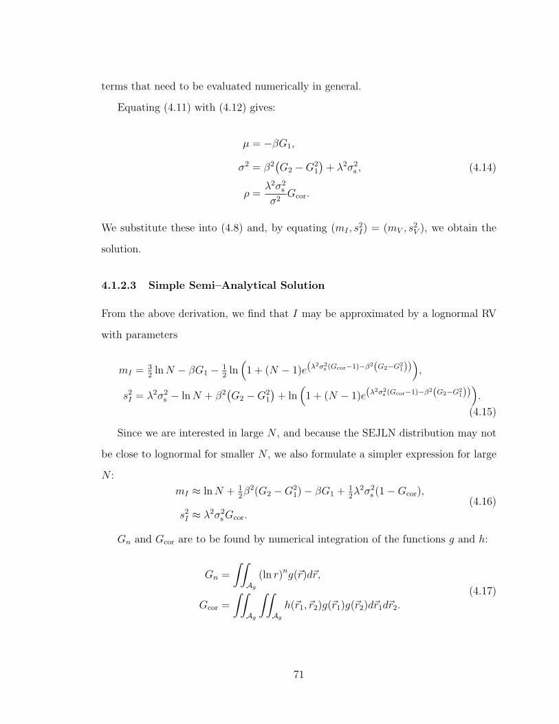
terms that need to be evaluated numerically in general.

Equating (4.11) with (4.12) gives:

µ = −βG1,

σ2 = β2(G2 −G2

1

)+ λ2σ2

s ,

ρ =λ2σ2

s

σ2Gcor.

(4.14)

We substitute these into (4.8) and, by equating (mI , s2I) = (mV , s

2V ), we obtain the

solution.

4.1.2.3 Simple Semi–Analytical Solution

From the above derivation, we find that I may be approximated by a lognormal RV

with parameters

mI = 32

lnN − βG1 − 12

ln(

1 + (N − 1)e(λ2σ2

s (Gcor−1)−β2(G2−G21))),

s2I = λ2σ2s − lnN + β2

(G2 −G2

1

)+ ln

(1 + (N − 1)e(λ

2σ2s (Gcor−1)−β2(G2−G2

1))).

(4.15)

Since we are interested in large N , and because the SEJLN distribution may not

be close to lognormal for smaller N , we also formulate a simpler expression for large

N :

mI ≈ lnN + 12β2(G2 −G2

1) − βG1 + 12λ2σ2

s (1 −Gcor),

s2I ≈ λ2σ2sGcor.

(4.16)

Gn and Gcor are to be found by numerical integration of the functions g and h:

Gn =

∫∫Ag

(ln r)ng(r)dr,

Gcor =

∫∫Ag

∫∫Ag

h(r1, r2)g(r1)g(r2)dr1dr2.

(4.17)

71

These integrals are well-behaved and can be well approximated by a Riemann sum

(trapezoidal rule) with a moderate number of terms. Gn and Gcor are termed “ge-

ometric coefficients”, and are an idea borrowed from [158, 159]. It should be noted

that this numerical integration is inevitable, due to the limitless possibilities for the

expressions of the functions g and h. However, our solution is elegant in that it sep-

arates these integrals from the scalar quantities β, σs, and N , in which it is purely

analytical. For this reason, and the brevity of the final equations, we believe this

solution to be the simplest possible while not being simplistic.

Another important point to observe in our solution is that only one scalar quantity

depends on the shadowing correlation function h, namely Gcor. This implies a large

loss of information about the channel model, which leads us to formulate a guideline:

while it is very important to include correlation in our model, only Gcor = E {h(r1, r2)}

(where r1, r2 are iid according to g(r)) is relevant to the analysis, which is much easier

to measure and estimate than all of h. In general, we think this kind of analysis can

point the way for engineers doing channel measurements to know what statistics are

actually relevant to particular problems, thus greatly reducing measurement efforts.

We may interpret this result through Theorem 4: indeed, it would seem that each

shadowing term is approximately composed of a lognormal component with spread√Gcorσs common to every path, as well as an additional lognormal term that is iid for

every path. As the paths add, the common term remains, while the iid terms vanish

as a consequence of the LLN, which is similar to our proof of the convergence of

the SEJLN distribution. This interpretation is also coherent with the physical model

presented in Figure 2.5.

72

4.2 Study of Moments

We now study the first two moments of the total interference I. This approach is

interesting for three reasons:

1. The moments (of positive integer order) are probably the easiest statistics to

derive in such problems.

2. The study of interference problems has historically started with moment analysis

[13], which has yielded good initial information.

3. The study of these moments gives us valuable insight into the asymptotic (as

N → ∞) behaviour of I, which shows the importance of modeling correlation

in shadowing, and also leads to some useful equations that can simplify lengthy

simulations, as seen in Section 5.3.6.

4.2.1 Formulation of Moments

We begin by evaluating the following quantities:

A = E {I1} = E{p(r1)e

λS1},

B = E{I21}

= E{p2(r1)e

2λS1},

C = E {I1I2} = E{p(r1)p(r2)e

λ(S1+S2)}.

(4.18)

Now, while the set {Si|ri} is not exchangeable, since the RVs may have differ-

ent variances, and pairs may have different correlation coefficients, the set {Si} is

exchangeable, and so is {Ii}. From this, we may easily formulate the moments:

E {I} = NA,

E{I2}

= NB +(N2 −N

)C,

VAR {I} = N(B − C) + N2(C − A2

).

(4.19)

73

We observe that, while for independent shadowing we have C = A2 ⇒ VAR {I} =

O(N), in general for correlated shadowing VAR {I} = O(N2). The mean power of I

remains the same regardless of correlation. Therefore what was already observed for

small N [155] will be even more significant for large N : adding correlation changes

(specifically, broadens) the distribution of I significantly. It follows that, given a suf-

ficiently realistic shadowing correlation model, the distribution of I obtained using

correlated shadowing will be much more realistic than that obtained using indepen-

dent shadowing.

Also, because of the asymptotic behaviour of the mean and variance, analysing I

as N → ∞ requires the study of the convergence of I/N (rather than (I − E {I})/√N

in the independent case). Because of the existence of correlation, the CLT cannot

be applied for large N . Indeed I/N does not necessarily converge to a Gaussian

distribution, and may in fact converge to a distribution close to a lognormal with a

significant spread, as we see in Section 5.2.3.

We can therefore conclude that correlation in shadowing becomes a dominating

factor in the distribution of I as N becomes large.

4.2.2 Numerical Evaluation of Moments

While we may estimate the expectations of (4.18) via Monte Carlo simulation, we

find it faster and more exact to evaluate them through numerical integration. By

first conditioning on r1 we have:

A =

∫ rmax

rmin

g(r)p(r)e12λ2σ2

s (r)dr, (4.20)

where g(r) is the pdf of ri, evaluated from g(r) as follows:

g(r) = r

∫ 2π

0

g(r)d∠r. (4.21)

74

Similarly,

B =

∫ rmax

rmin

g(r)p2(r)e2λ2σ2

s (r)dr. (4.22)

Finally,

C =

∫∫Ag

∫∫Ag

g(r1)g(r2)p(r1)p(r2)r1r2eλ2

(12σ2s (r1)+

12σ2s (r2)+σs(r1)σs(r2)h(r1,r2)

)dr1dr2.

(4.23)

This integral needs to be evaluated in four dimensions for a general correlation model

h, and is not easy to separate in the case of model (3.5).

4.2.3 Using Moments in the Large–N Regime

Having described a fairly straightforward method for obtaining the first two moments

of I, we may use this information to assist in finding the approximate distribution

of I when N is large. To do this, consider first the limiting distribution of I/N as

N → ∞. While we do not know the shape of this distribution, we may conjecture

that such a limiting distribution exists, since I is the sum of exchangeable RVs [64].

It is not necessary to know anything about the shape of this limiting distribution

to see that, once N is large enough, one would expect the shape of the cdf of I to

stabilise, and the cdf merely shift according to N . This leads to the following two

related ideas:

1. If we know the distribution of I for some large N (e.g., through simulation),

we may extrapolate its behaviour for some larger number of interferers NM

(M > 1), using knowledge of moments to shift the cdf appropriately while

maintaining its shape.

2. Conversely, if we obtain the limiting distribution of I/N as N → ∞ (which we

at this point do not know how to do), the distribution of I for some large N

can likewise be approximated by shifting the limiting distribution appropriately

75

using the knowledge of moments.

In both cases, we derive equations that apply some affine (linear plus constant)

transformation to a known cdf in order to obtain the cdf of I for some different large

N . The linear transformation preserves the shape in the linear and dB domains,

but the added constant will deform the shape in the case of the dB domain only.

To achieve these transformations, three methods present themselves: using the mean

only, using the variance only, and using both. We will explore this approach in detail

in Section 5.3.6.

4.2.3.1 Mean–Matching

The case of mean–matching is the simplest, as the mean of I is simply proportional

to N , and we need not compute the moments of I explicitly. We then have

NM∑i=1

IiD≈ M

N∑i=1

Ii, M ≥ 1, N large, (4.24)

andN∑i=1

IiD≈ N

(limN ′→∞

1

N ′

N ′∑j=1

Ij

), N large, (4.25)

two simple expressions to shift the cdf of I within the large–N regime.

4.2.3.2 Variance–Matching

A different linear transformation may be obtained by matching not the mean, but

only the variance between the available and desired distributions. In this case we also

have a finite and asymptotic version.

In the finite case, we have

NM∑i=1

IiD≈ c

N∑i=1

Ii, M ≥ 1, N large, (4.26)

76

where

c =

√NM(B − C) + N2M2(C − A2)

N(B − C) + N2(C − A2). (4.27)

Now, in the asymptotic case, we observe that

VAR {I/N} −→ C − A2, as N → ∞. (4.28)

It follows thatN∑i=1

IiD≈ c′

(limN ′→∞

1

N ′

N ′∑j=1

Ij

), N large, (4.29)

where

c′ =

√N2 + N

B − C

C − A2. (4.30)

Variance–matching is not very different from mean–matching, in that they both

multiply the data by a constant factor, and c ≈ M and c′ ≈ N for high N .

4.2.3.3 Matching both Mean and Variance

Since the first two moments of I are always easily obtainable from (4.19), the scaling

approach can be refined using both moments in the following respective ways:

NM∑i=1

IiD≈ b + a

N∑i=1

Ii, M ≥ 1, N large, (4.31)

where

a =

√M(B − C + NM(C − A2))

B − C + N(C − A2),

b = NA(M − a).

(4.32)

77

Similarly, beginning with

E {I/N} −→ A,

E{

(I/N)2}−→ C,

VAR {I/N} −→ C − A2, as N → ∞,

(4.33)

we obtainN∑i=1

IiD≈ b′ + a′

(limN ′→∞

1

N ′

N ′∑j=1

Ij

), N large, (4.34)

where

a′ = c′ in (4.30),

b′ = A(N − a′).(4.35)

Again, this matching is not very different from the previous approaches, since for

large N we have a′ approaching N and b′ approaching zero. An important difference

is that adding the b′ term does not allow the approximating distribution to take values

in the neighbourhood of zero, which may cause high relative error in the lower tail.

4.3 Problem Reformulation Using a Stochastic Integral

It would be interesting to actually find the limiting distribution of I/N . While we do

not have a solution to this problem, we offer here a reformulation of the problem from

an infinite sum into a stochastic integral that does not depend on N , which might be

a first step towards the analysis of this problem.

This reformulation also motivates an alternative simulation algorithm, namely

shadowing fields, which proves computationally efficient for high N , and is described

in Section 5.3.1.

78

4.3.1 Equivalent Stochastic Integral for I/N as N → ∞

Consider a two–dimensional Gaussian shadowing field S(r), r ∈ R2 \ 0, such that if

we assign Si = S(ri), then the Si’s have the desired joint distribution. Then S(r) is

a stochastic field. Now, as we observe that since the values Si essentially sample this

random field, the expression for I is actually a stochastic numerical integration of a

function of S(r). The corresponding integral would take the following form:

I

N

D−→∫R2

g(r)p(∥r∥)eλS(r)dr as N → ∞. (4.36)

4.3.2 Mathematical Argument

The following is not an exact proof, as the convergence of various quantities is not

proved but assumed. The argument assumes that S(r) is correlated enough so that

small variations in r give correspondingly small variations in S(r): this is probably

the case for the model (3.5), but not if shadowing is, e.g., independent.

Consider a square region A of side length δ such that Ag ⊂ A, and divide A into

L × L uniform square regions Al, l = 1, . . . , L2. Also, let ql be the centre of square

Al. Let us fix N = L3 and let L → ∞.

We have

I

N=

1

N

N∑i=1

p(ri)eλSi = L−3

L2∑l=1

Jl∑j=1

p(rl,j)eλSl,j , (4.37)

where the indices have been remapped as i 7→ l, j, such that for every l, rl,j ∈ Al.

Since N → ∞ ⇒ L → ∞ ⇒ ∥rl,j − ql∥ < δ/√

2L → 0, we can now make the

following approximations:

p(rl,j) ≈ p(ql), (4.38)

where ql = ∥ql∥, and assuming p(r) does not vary too quickly over a small distance.

79

Also,

Sl,j = S(rl,j) ≈ S(ql) = Sl, (4.39)

assuming that σs(r) does not change too quickly over a small distance, and from the

fact that the values of S(r) at two nearby points have a correlation coefficient close

to 1. We then have S(r) almost constant over Al with high probability.

These two approximations lead to:

I

N≈ L−3

L2∑l=1

p(ql)eλSlJl. (4.40)

Now Jl is a binomial RV with parameters L3 and∫Al

g(r)dr ≈ g(ql)δ2/L2, and

therefore

E {Jl/L} = g(ql)δ2,

VAR {Jl/L} = L−1g(ql)δ2(1 − g(ql)δ

2/L2)≈ L−1g(ql)δ

2.(4.41)

We observe that the variance of Jl/L is O(L−1) and hence vanishes. It follows

that the quantity converges in distribution to its mean (this is a similar argument to

the one used in the proof of the LLN [61, p.275]), and we may write:

I

N≈ (δ/L)2

L2∑l=1

p(ql)eλSlg(ql). (4.42)

This last expression, as L → ∞, is essentially a Riemann integral expression of (4.36).

4.4 Summary

Various analytical tools can help with the derivation of the approximate distribution

of I. We follow with a chapter on simulation, where we show how these approximate

solutions perform against Monte Carlo simulations, and also show how some analytical

results may assist in the accelerated simulation of said distribution.

80

Chapter 5

Simulation Results and Optimisation

Simulation carries significant weight in our work. On the one hand, we use Monte

Carlo simulation to verify the accuracy of the approximate solution for the distribu-

tion of I developed in Section 4.1. On the other hand, our analytical solution proves

accurate only in certain cases, and we may need to resort to a simulation approach

in general. To this end, we find that we can greatly simplify the Monte Carlo sim-

ulations via various analytical results from Sections 4.2 and 4.3, thus resulting in a

mixed simulation–numerical–analytical method.

These two approaches really serve to solve the same problem: how to find the dis-

tribution of I as quickly as possible and with good accuracy, by any means necessary.

5.1 Simulation Setup

We begin by describing the basic simulator used to obtain the cdf of I via Monte

Carlo simulation.

5.1.1 Simulation Platform

We now describe the software and hardware parameters used to perform the sim-

ulations in this thesis. These are of particular interest when we examine the time

81

performance of various simulation algorithms in Section 5.3. However, we do not

expect the relative time gains between different simulation setups to vary much, for

two reasons:

1. The relative simulation times tend to roughly correspond to what would be

expected theoretically.

2. We spent a significant amount of time optimising the simulation code, so that

the majority of computational time is devoted to mathematical operations and

not software overhead.

The hardware and software specifications of the simulation platform are as follows:

• Intel R⃝ CoreTMi7 860, 2.8GHz, 8 logical cores (4 physical cores with hyper–

threading).

• 8 GB RAM.

• Microsoft R⃝ Windows R⃝ 7 Professional, 64 bit.

• The MathWorksTM MATLAB R⃝ version 7.9.0.529 (R2009b).

We observed that MATLAB automatically uses several of the logical cores in parallel

to execute large repetitive tasks. The repetitive nature of the algorithms lends itself

particularly well to hardware parallelisation.

5.1.2 Traditional Approach: Matrix Factorisation

The principle challenge in the Monte Carlo simulation of I is the joint simulation of

S given {ri}Ni=1. Generating a Gaussian vector of arbitrary correlation matrix K is

often [48,57,102,113,160,161] done by solving for CN×N in the equation

K = CTC, (5.1)

82

for each particular realisation of K. We write C = ∗√K. The next step is to generate a

vector Z = [Zi]Ni=1 of independent standard Gaussian N (0, 1) RVs. S is then obtained

from

S = ZC. (5.2)

This is implemented as follows:

Algorithm using Matrix Factorisation

Ensure: The histogram of I[k] approximates the pdf of I.

for k = 1 to K do

for i = 1 to N do

ri ⇐ i.i.d. random from g(r)

Zi ⇐ i.i.d. random N (0, 1)

end for

for i = 1 to N do

K[i, i] ⇐ 1

for j = 1 to i− 1 do

K[i, j] = K[j, i] ⇐ h(ri, rj)

end for

end for

C ⇐ ∗√K

S ⇐ diag(σs(r1), . . . , σs(rN)) · Z · C

I[k] ⇐∑N

i=1 p(ri)eλSi

end for

There exist various algorithms for calculating C. In the case when K is positive

definite, Cholesky factorisation is a stable algorithm [113,160] that gives a triangular

83

solution for C. However, K is allowed to be psd in general1. Also, numerical rounding

can make K slightly non–psd. To fix this double problem there are at least two

procedures. One is to modify K slightly so that it becomes positive definite [113].

However, K need not be positive definite (as suggested in [57, 102, 113]), but may

be psd in general. In this case, Cholesky factorisation is not applicable, and matrix

diagonalisation (eigenvalue decomposition) [66, 70, 114, 142] should be used. Also,

should some of the resulting eigenvalues of K be slightly negative due to rounding,

they can be set to zero [114]. Then, if there are eigenvalues equal to zero, K is not

full rank and therefore not positive definite, but C can still be found. Additionally,

if K is highly–correlated, a fast approximation exists [162].

While Cholesky factorisation fails for singular matrices K, we have observed in

simulations that this event is extremely rare using model (3.5) with double–precision

arithmetic. Therefore, we simply use Cholesky factorisation, and reject the extremely

rare simulations where this method fails.

5.1.3 Representing the Simulation Results

To obtain an accurate estimate of the cdf of I, we generate K = 1 000 000 trials

of I, and plot their empirical cdfs. This tends to give smooth curves at least in the

probability interval [10−4, 1 − 10−4]. The cdf is plotted on “lognormal paper” [157], on

which the axes are deformed in such a way that all (and only) lognormal distributions

appear as straight lines with positive slope. This is becoming common practice in

interference work [22, 23], and is useful in our case, since we propose a lognormal

approximation to the distribution of I; thus, we can evaluate whether a lognormal

approximation is possible by looking at the linearity of the estimated cdf on lognormal

paper.

1The case when K is psd but not positive definite corresponds to a singular matrix. In practice,for randomly generated positions ri and using double–precision arithmetic, we find this event to beextremely rare in our simulations, and thus Cholesky factorisation is almost safe.

84

−140 −120 −100 −80 −60 −40 −20 1e−5

1e−4

0.001

0.01

0.1

0.5

0.9

0.99

0.999

1−1e−4

1−1e−5

dB

N = 1 2 10 100 500

Correlated ShadowingIndependent Shadowing

Figure 5.1: Interference cdfs on lognormal paper: with and without shadowing cor-relation.

85

5.1.4 Correlated versus Independent Shadowing

As a first exercise, let us observe the interference cdfs as obtained from the described

simulation approach. We compare these empirical cdfs to those obtained from assum-

ing only independent shadowing, but with the same marginal distribution. Figure 5.1

illustrates this comparison for varying N . While for N = 1 the obtained cdfs are

essentially the same (theoretically, they are identical, since there is no correlation

among just one IS), and while for small N correlation does not change the cdf sig-

nificantly, for higher N the gap increases between the cdf using independent versus

correlated shadowing. Specifically, we observe a broadening of the cdf when correla-

tion is included, with respect to the cdf obtained using independent shadowing, an

effect which increases with N . This is expected from the rate of growth of the variance

of I, as predicted from (4.19). This supports our claim that shadowing correlation

should not be neglected when studying the interference from large networks.

5.2 Evaluating the Accuracy of the Lognormal Approxima-

tion Method

In Section 4.1.2 we developed a simple semi–analytical approximation to the distribu-

tion of I. The argument is predicated on the convergence of the SEJLN distribution

to a lognormal. We first test the accuracy and rate of convergence of this claim, after

which we evaluate how well, and in what cases, our semi–analytical solution works.

5.2.1 Accuracy of Convergence of the SEJLN Distribution to the Log-

normal

Equations (4.8) and (4.9) both give, with a different degree of accuracy, the param-

eters of a lognormal approximation to the SEJLN distribution. We wish to evaluate

the validity of these approximations as a function of the SEJLN parameters. Since

86

eµ is a scaling factor, we may set µ = 0 without loss of generality. We then fix the

parameters ρ and σ and increase N . We show simulations for σ = 6 dB and 12 dB,

and for ρ = 0.5, 0.05, and 0.005. Note that for the equations to apply, the value

of σ must be converted from dB to natural units as follows: σ[ nat] = λ × σ[ dB].

Therefore, σ ∼= 1.382 and 2.763.

In Figures 5.2 through 5.7, we show Monte Carlo simulations of the SEJLN distri-

bution computed using (4.4), which is an exact algorithm for simulating the SEJLN

distribution in O(N) time. We compare the simulations to the lognormals with pa-

rameters (4.8) and (4.9). We plot the distributions on lognormal paper to evaluate

the convergence to the lognormal distribution.

We can make the following observations from these figures:

1. As per our theorem, for all 0 < ρ ≤ 1 and σ2 = 0, the SEJLN distribution tends

toward a lognormal distribution with known parameters as N → ∞.

2. The SEJLN distribution is (trivially) lognormal for N = 1. For N ≥ 2, the

SEJLN distribution becomes less and less lognormal until a certain N , and

then begins to converge back to a lognormal distribution. Once it is again

approximately lognormal for a certain N , it remains approximately lognormal

for any larger N .

3. The convergence of the SEJLN to a lognormal is faster for higher ρ and for

lower σ.

4. Though the SEJLN distribution converges to a lognormal, this convergence

is not uniform over the whole range of values and in fact never converges at

arbitrarily large values, where the behaviour is instead known to be that of

the heaviest term in the sum times the number of these heaviest terms, for

−1 ≤ ρ < 1 (as long as the matrix remains psd) [17]. This is notably visible in

87

−20 −10 0 10 20 30 40 50 1e−5

1e−4

0.001

0.01

0.1

0.5

0.9

0.99

0.999

1−1e−4

1−1e−5

dB

SimulationLognormal Approximation − AsymptoticLognormal Approximation − Exact

10

12 5

1001000 10000

Figure 5.2: SEJLN cdf on lognormal paper, σ = 6 dB, ρ = 0.5, with varying N .

88

−10 0 10 20 30 40 50 1e−5

1e−4

0.001

0.01

0.1

0.5

0.9

0.99

0.999

1−1e−4

1−1e−5

dB

SimulationLognormal Approximation − AsymptoticLognormal Approximation − Exact

210

100 1000 10000

Figure 5.3: SEJLN cdf on lognormal paper, σ = 6 dB, ρ = 0.05, with varying N .

89

0 5 10 15 20 25 30 35 40 45 50 1e−5

1e−4

0.001

0.01

0.1

0.5

0.9

0.99

0.999

1−1e−4

1−1e−5

dB

SimulationLognormal Approximation − AsymptoticLognormal Approximation − Exact

10 100 1000 10000

Figure 5.4: SEJLN cdf on lognormal paper, σ = 6 dB, ρ = 0.005, with varying N .

90

−40 −20 0 20 40 60 80 1e−5

1e−4

0.001

0.01

0.1

0.5

0.9

0.99

0.999

1−1e−4

1−1e−5

dB

SimulationLognormal Approximation − AsymptoticLognormal Approximation − Exact

2 10

1001000

10000

Figure 5.5: SEJLN cdf on lognormal paper, σ = 12 dB, ρ = 0.5, with varying N .

91

20 30 40 50 60 70 80 1e−5

1e−4

0.001

0.01

0.1

0.5

0.9

0.99

0.999

1−1e−4

1−1e−5

dB

SimulationLognormal Approximation − AsymptoticLognormal Approximation − Exact

100 100010000 100000

Figure 5.6: SEJLN cdf on lognormal paper, σ = 12 dB, ρ = 0.05, with varying N .

92

50 55 60 65 70 75 80 85 1e−5

1e−4

0.001

0.01

0.1

0.5

0.9

0.99

0.999

1−1e−4

1−1e−5

dB

SimulationLognormal Approximation − AsymptoticLognormal Approximation − Exact

10000100000

1000000

Figure 5.7: SEJLN cdf on lognormal paper, σ = 12 dB, ρ = 0.005, with varying N .

93

Table 5.1: Geometric coefficients for each layout in Figure 3.1.

Layout: G1 G2 −G21 Gcor

A : Square Cluster 5.866 0.06763 0.5775

B : Gaussian Cluster 5.617 0.04369 0.6701

C : Surrounding Ring 5.738 0.1959 0.1138

D : Surrounding Thin Ring 6.215 3.331 · 10−9 0.1667 ∼= 16

Figure 5.7. This is not in contradiction with our result, since we have proved

convergence in distribution, i.e., convergence at every point x (see Definition

14), but not necessarily in the limit behaviour as x → ∞.

We have thus confirmed the convergence of the SEJLN distribution to the lognor-

mal, and have given a general feel for the rate of this convergence as a function of ρ

and σ. We now verify the accuracy of its application to finding the distribution of I.

5.2.2 Numerical Evaluation of the Geometric Coefficients

The first step in finding the approximating distribution to that of I is to evaluate the

necessary geometric coefficients G1, G2, and Gcor. The first two coefficients depend

only on g(r), and may therefore be computed directly for any layout, while the last

coefficient, Gcor, also requires the knowledge of the correlation model. To evaluate

Gcor, we choose the same model described in Section 3.2.3 and shown in Figure 3.2.

Table 5.1 gives the geometric coefficients for every layout in Figure 3.1. Some

details on how to compute these values in practice follow:

• For most coefficients, it is sufficient to evaluate the integrals in (4.17) directly

via Riemann integration. However, we find it more judicious to evaluate G1

and G2 − G21 (which can be interpreted as a mean and variance of ln r respec-

tively), since this second quantity is often quite small compared to G2, and

94

the expressions are very sensitive to rounding errors. We find that 1000 uni-

form integration steps per dimension for Gn, and 50 steps per dimension for

Gcor, are sufficient for the integral to converge (given that for a higher num-

ber of steps, the integrals remain within 1%). The computational time for

evaluating all three coefficients is around 1.5 seconds, and represents the only

computationally–intensive step of our method.

• Finding Gcor in Layout D directly through Riemann integration is not practical,

as the ring is so thin that most points on the grid would not land inside it.

Instead, when we consider that between r = 499.9 and r = 500 we have the

dB ratio R ∼= 0.00087, which corresponds to a negligible relative difference of

0.00014 in the correlation coefficient when R0 = 6 dB, we may approximate

h(r1, r2) ∼= h(θ) = max {1 − θ/θ0, 0}. This leads to the approximation

Gcor∼=(

1

π(r2max − r2min)

∫ rmin

rmax

rdr

)2

·∫ 2π

0

∫ 2π

0

h(θ)dθ1dθ2

=1

(2π)2

∫ 2π

0

∫ 2π

0

h(θ)dθ1dθ2 =1

2π

∫ π

−πmax

{1 − |θ1|

θ0, 0

}dθ1 =

θ02π

.

(5.3)

• For uniform annular regions (Layouts C and D), it is simple to evaluate Gn

analytically. We may rewrite, from (4.17),

Gn =2

r2max − r2min

∫ rmax

rmin

(ln r)nrdr ⇒

G1 =r2max

(ln rmax − 1

2

)− r2min

(ln rmin − 1

2

)r2max − r2min

,

G2 =r2max

((ln rmax − 1) ln rmax + 1

2

)− r2min

((ln rmin − 1) ln rmin + 1

2

)r2max − r2min

.

(5.4)

We now examine how well the resulting lognormal approximation performs, first

for clustered, then for non–clustered geometries.

95

5.2.3 Lognormal Approximation to I in a Clustered Layout

We begin with the clustered layouts, which are A and B in Figure 3.1. Both have a

high average shadowing correlation Gcor > 0.5, and a rather small spread of values

of r (a useful metric for this is√

G2 −G21/G1). We make the approximation that

the shadowing spread is constant: σs, and the average pathloss is power law with

exponent β. We may therefore apply the lognormal approximations in (4.8) and

(4.9). The results are shown in Figures 5.8–5.11.

If we look back at simulations of the SEJLN cdf for ρ = 0.5 (Figures 5.2 and 5.5),

we observe that the convergence to a lognormal cdf is very good for N = 1000, and

indeed even for smaller N . If we assume that the SEJLN problem can be mapped onto

the problem of the distribution of I, we would expect a similar behaviour. Indeed

the convergence is almost exact in the case of Layout A (Figures 5.8 and 5.9), while

in the case of Layout B it is somewhat inexact at the lower tail, as we see that the

cdf is not quite lognormal. The accuracy of the method rapidly deteriorates when we

switch to non–cluster layouts with lower average correlation.

5.2.4 Lognormal Approximation to I in a Non–Clustered Layout

We now examine the performance of our approximations in the case of Layout C. The

simulations are again performed assuming constant shadowing spread and pathloss

exponent. The results in Figure 5.12 confirm that our method does not perform at

all well in this case.

Now, recall that the convergence of the SEJLN to a lognormal distribution is

proved exactly. When we translate the problem to that of the distribution of I, we

make two approximations: we assume that each Ii has a lognormal distribution, and

we assume that {Ii} is a jointly lognormal set. It would be interesting to understand

the effects of these two approximations to explain the failure of the approximation

96

−140 −130 −120 −110 −100 −90 −80 −70 −60 −50 −40 1e−5

1e−4

0.001

0.01

0.1

0.5

0.9

0.99

0.999

1−1e−4

1−1e−5

dB

SimulationLognormal Approximation − AsymptoticLognormal Approximation − Exact

Figure 5.8: Total interference cdf on lognormal paper for Layout A, with σs = 6 dB,β = 4, and N = 1, 10, 100, 1000 from left to right.

97

−140 −120 −100 −80 −60 −40 −20 0 20 1e−5

1e−4

0.001

0.01

0.1

0.5

0.9

0.99

0.999

1−1e−4

1−1e−5

dB

SimulationLognormal Approximation − AsymptoticLognormal Approximation − Exact

Figure 5.9: Total interference cdf on lognormal paper for Layout A, with σs = 12 dB,β = 3, and N = 1, 10, 100, 1000 from left to right.

98

−110 −100 −90 −80 −70 −60 −50 −40 −30 −20 −10 1e−5

1e−4

0.001

0.01

0.1

0.5

0.9

0.99

0.999

1−1e−4

1−1e−5

dB

SimulationLognormal Approximation − AsymptoticLognormal Approximation − Exact

Figure 5.10: Total interference cdf on lognormal paper for Layout B, with σs = 6 dB,β = 3, and N = 1, 10, 100, 1000 from left to right.

99

−160 −140 −120 −100 −80 −60 −40 −20 1e−5

1e−4

0.001

0.01

0.1

0.5

0.9

0.99

0.999

1−1e−4

1−1e−5

dB

SimulationLognormal Approximation − AsymptoticLognormal Approximation − Exact

Figure 5.11: Total interference cdf on lognormal paper for Layout B, with σs = 12 dB,β = 4, and N = 1, 10, 100, 1000 from left to right.

100

−140 −120 −100 −80 −60 −40 1e−5

1e−4

0.001

0.01

0.1

0.5

0.9

0.99

0.999

1−1e−4

1−1e−5

dB

SimulationLognormal Approximation − AsymptoticLognormal Approximation − Exact

Figure 5.12: Total interference cdf on lognormal paper for Layout C, with σs = 6 dB,β = 4, and N = 1, 10, 100, 1000 from left to right.

101

−140 −130 −120 −110 −100 −90 −80 −70 −60 −50 1e−5

1e−4

0.001

0.01

0.1

0.5

0.9

0.99

0.999

1−1e−4

1−1e−5

dB

SimulationLognormal Approximation − AsymptoticLognormal Approximation − Exact

Figure 5.13: Total interference cdf on lognormal paper for Layout D, with σs = 6 dB,β = 4, and N = 1, 10, 100, 1000 from left to right.

102

in some cases. Firstly, it can be observed from Figure 5.12 for N = 1 that Ii is

not close to a lognormal. The question is: does jointness even matter? To evaluate

this, we consider Layout D (admittedly an artificial case), where we see that r is

quasi–constant, and the total interference is well approximated by

I ≈ (499.95)−βN∑i=1

eλSi , (5.5)

which, when σs is constant, is exactly a sum of lognormals (but not jointly lognormal!)

formulation. We observe the simulation results in Figure 5.13. In the case of N = 1,

we indeed observe that Ii is almost perfectly lognormal. However, for N = 1000,

we observe that the distribution of I is not close to lognormal. In this case we have

σ[ dB]] ∼= σs = 6 dB and ρ ∼= Gcor = 0.1667. Looking back at Figure 5.3, where σ is

the same, and ρ is lower, we still observe almost perfect convergence when N = 1000;

we would therefore expect even better convergence for ρ = 0.1667, but Figure 5.13

contradicts this.

Because the only difference between (5.5) and the SEJLN problem is jointness, we

may conclude that lack of jointness in {Si} is a significant impediment to our method.

Indeed, we observe in the next section that, in the case of Layout C, while the cdf of

I does indeed converge, it is not to a lognormal. A different, multi–faceted approach

is required to solve the general problem of the distribution of I.

5.3 Simulating I Rapidly: Combined Simulation–Numerical–

Analytical Approach

The lognormal approximation, combined with the cross–moment matching approach,

yields a good approximation for a good subset of large interference problems, but it

is clearly inadequate in the general case. The complexity of finding the distribution

103

Table 5.2: Simulation settings after calibration.

Parameter Value

Physical Parameters

g(r) Layout C

rmin 50

rmax 500

p(r) r−2(1 + r/150)−2

σs(r) 10(1 − exp (−3r/200)) dB

h(r1, r2) max {1 − θ/θ0, 0} · max {1 −R/R0, 0}θ0 60◦

R0 6 dB

Simulator Parameters

K 1 000 000

Kr 10 000

KCh 10 000

DΘ 12

DR 10

FΘ 2

FR 6

104

of I in the general case may be too daunting. Simultaneously, the simulation of I for

large N is very costly in computational time and memory. In this section, we show

how we can approximate the distribution of I well (within 1 dB) and quickly (over

1000 times faster for large N), using a combination of Monte Carlo simulation, image

processing techniques, numerical integration, and analytical results.

To this end, we first describe the use of shadowing fields in general, and how they

can bring the computational complexity down to O(N); we also show their particular

applicability to the correlation model described in (3.5). We then examine how a

judicious reuse of random samples can accelerate the computation by an order of

magnitude or more. Finally, we show how to use the equations derived in Section

4.2.3 to extrapolate the distribution of I for very large N from smaller simulations.

The simulations in this section are performed using the parameters in Table 5.2.

The simulator parameters are adjusted through a calibration process, which we de-

scribe in Section 5.3.4.

5.3.1 Shadowing Fields

A shadowing field is a random field in two dimensions, such that it is a Gaussian

(given lognormal shadowing) process with a specific auto–correlation function. This

auto–correlation is such that, when interferers with positions ri are placed on the

field, and the value of the field at the point ri is taken as the value of Si, then

S|r1, . . . , rN has the desired correlation matrix K. This can be compared by analogy

to gravitational (electric, etc.) fields, where the field gives the acceleration of a mass

placed at any point, whether there actually is a mass at that point or not.

The idea of generating shadowing fields has already been explored [37, 38, 40, 42]

with correlation functions of the form h(d). We have argued in Section 2.5 that

such models may not reflect true shadowing spatial correlation characteristics. Fur-

thermore, correlation as a separable function of θ and R can be easily simulated by

105

a) b)

c) d)

−3 −2 −1 0 1 2 3

Figure 5.14: Shadowing field realisations for rmin = 50, rmax = 500, θ0 = 60◦, R0 =6 dB, with increasing resolution: DΘ = 6n,DR = 5n, FΘ = n, FR = 3n, where a)n = 1, b) n = 2, c) n = 5, d) n = 50. The colour of the areas corresponds to thevalue of Si/σs(ri) therein.

106

using a geometric transformation. The accuracy of our method is limited only by the

quantisation level.

Consider a random field (a two–dimensional RP) M of continuous parameters

(x, y). Let the random field be stationary, with an auto–correlation function such that

the correlation between the field at two points, M(xi, yi) and M(xj, yj), correspond

to the desired shadowing correlation under some transformation.

Consider what we call the log–polar2 transformation:

TLP : (θ, R) 7−→ 100.1R(cos θ, sin θ),

TLP : [0, 2π] × [10 log10 rmin, 10 log10 rmax] 7−→ {r : rmin ≤ r ≤ rmax}.(5.6)

Let us choose the auto–correlation of M as

ηx(ξ) =

1 − |ξ|/θ0 |ξ| ≤ θ0,

0 θ0 ≤ |ξ| ≤ 2π − θ0,

1 + (|ξ| − 2π)/θ0 2π − θ0 ≤ |ξ| ≤ 2π.

ηy(υ) =

1 − |υ|/R0 |υ| ≤ R0,

0 |υ| > R0,

E{M(x + ξ, y + υ)M(x, y)

}= ηx(ξ)ηy(υ),

(5.7)

for M defined on [0, 2π]× [10 log10 rmin, 10 log10 rmax]. We find that the field M, under

transformation TLP, has the correlation properties of (3.5), i.e.,

TLP : (xi, yi) 7−→ ri, i = 1, 2, . . .

E{M(x1, y1)M(x2, y2)

}= h(r1, r2).

(5.8)

2A polar representation of certain shadowing fields is suggested in [37].

107

Therefore, we may write

Si = S(ri) = σs(ri)M(T −1LP (ri)

), (5.9)

and Si’s have the same correlation matrix as in (5.2), while S(r) is the same stochastic

process as described in Section 4.3.

For numerical purposes, M can be approximated by a discrete–parameter matrix

MDΘ×DR, with a regularly–spaced quantisation grid along θ and R. Correlation of

the form (3.5), triangular in both dimensions, can be obtained by using a uniform

square filter FFΘ×FR, ideally choosing FΘ and FR so that we have exactly

FΘ/DΘ = θ0/2π,

FR/DR = R0/10 log10 (rmax/rmin),(5.10)

with F equal everywhere to 1/√FΘFR.

To obtain the value of the discretised field M at some point, we must round

the coordinates T −1LP (ri) to the nearest quantisation point. Therefore the algorithm

is limited in precision by the finite spatial quantisation. On the other hand, the

computational cost of generating one field grows as O(FΘFRDΘDR) = O(D2ΘD

2R),

and so it is critical to choose the number of quantisation points DΘDR properly to

balance precision and computational time. Figure 5.14 shows realisations of the same

shadowing fields at different resolutions.

Shadowing fields have the additional advantages of requiring only O(N) mem-

ory (rather than O(N2) for matrix factorisation), and being able to accommodate

interferer mobility easily: indeed, while matrix factorisation only gives shadowing

values at the N specified locations, shadowing fields give the value of the (potential)

shadowing everywhere. This is also useful when N is uncertain, random, or variable.

108

5.3.2 Efficient Filtering for Separable Triangular Correlations

The choice of the correlation model (3.5) is particularly fortunate from the point of

view of computational efficiency, because it benefits from two properties: separability

and a triangular shape.

5.3.2.1 Separability

The nature of the correlation model (3.5) is such that it can be expressed as the

product of a function of θ and a function of R. It follows [60] that the resulting two–

dimensional process in the θ–R plane is also separable. It can therefore be simulated

by filtering over each dimension separately, which reduces the general filtering cost

from O(FΘFRDΘDR) (as in, e.g., [38]) to O((FΘ + FR)DΘDR).

5.3.2.2 Optimised Box Filters

The triangular form in θ and R of the correlation expression in (3.5) requires the use

of rectangular (box) filters applied to a white Gaussian process. Computationally

this is very efficient, as the filtering requires no multiplications. Additionally, it

can be implemented even more efficiently [163], with the number of additions now

approximately 2DΘ and 2DR in each respective dimension, rather than (FΘ − 1)DΘ

and (FR − 1)DR respectively. This is due to the fact that adjacent outputs of a box

filter differ only by two input values. This makes the total computation cost for one

field realisation O(DΘDR), which is independent of the filter size and hence of the

correlation distances θ0 and R0.

5.3.2.3 Optimised Shadow Fields Algorithm

A general shadowing fields algorithm would have such a form:

Basic Shadowing Field Algorithm

109

Ensure: The histogram of I[k] approximates the pdf of I.

for k = 1 to K do

for i = 1 to N do

ri ⇐ i.i.d. random from g(r)

end for

M ⇐ shadowing field realisation†

for i = 1 to N do

Si ⇐ σs(ri)M[T −1LP (ri)

](nearest index)

end for

I[k] ⇐∑N

i=1 p(ri)eλSi

end for

Now the correlation model (3.5) benefits from separability in the R and θ domains,

as well as from the triangular form of both auto–correlations. It is also important

to remember to wrap the field in the θ direction so as to ensure angular continuity.

These elements produce the following detailed implementation:

†Fast Shadowing Field Generation

Ensure: M is Gaussian, correlated approximately as (3.5).

ZDΘ×(DR+FR−1) ⇐ i.i.d. random N (0, 1)

Initialise a temporary matrix WDΘ×(DR+FR−1)

for m = 1 to DR + FR − 1 do

W[1,m] ⇐∑FΘ

n=1 Z[n,m]

end for

for n = 1 to DΘ − 1 do

n∗ ⇐ (n + FΘ − 1) mod DΘ + 1

for m = 1 to DR + FR − 1 do

W[n + 1,m] ⇐ W[n,m] − Z[n,m] + Z[n∗,m]

110

end for

end for

for n = 1 to DΘ do

M[n, 1] ⇐∑FR

m=1W[n,m]

end for

for m = 1 to DR − 1 do

for n = 1 to DΘ do

M[n,m + 1] ⇐ M[n,m] −W[n,m] + W[n,m + FR]

end for

end for

5.3.3 Reusing Random Samples

Converting the simulation algorithm from matrix factorisation to shadowing fields

can bring a great gain in simulation time for large N . We may, however, augment

these gains by using an additional technique, based on reusing random samples, that

can be applied to both algorithms to greatly decrease their computational time at a

negligible cost in accuracy.

We begin with the observation that both algorithms, while quite different, are also

fundamentally similar: both require the generation of NK positions from g(r), and

also the generation of a large set of independent Gaussian RVs. These RVs are then

linearly combined to obtain the required correlation structure, after which we may

compute Ii and I according to (3.6). We further observe that the generation of the

independent Gaussians and that of the interferer positions are two separate processes.

This leads to the idea of generating fewer random quantities of both kinds, and

pairing them in different combinations so as to achieve a similar amount of randomness

as if each realisation was different. We call Kr the number of times the positions of

111

the interferers are generated, for a total sample size of NKr from g(r). We also call

KCh the total number of channel realisations generated, though this has a somewhat

different meaning in both algorithms. We impose the following conditions:

K/Kr ∈ N∗,

K/KCh ∈ N∗,

KrKCh/K ∈ N∗.

(5.11)

An important implementation consideration is which of the two, positions or Gaus-

sians, to generate first, as these need to be stored in memory during the simulation to

allow for reuse. Let us examine the details of implementing reuse for each algorithm

separately.

5.3.3.1 Reuse in Matrix Factorisation

Matrix factorisation requires the generation and factorisation of Kr N ×N matrices,

but the generation of only N × KCh independent Gaussians. It is therefore more

judicious, for large N , to generate the Gaussian RVs first and store them for reuse,

and then to generate and discard the interferers’ positions and correlation matrices

one by one. This can be implemented as follows:

Matrix Factorisation Algorithm with Reuse

Ensure: The histogram of I[k] approximates the pdf of I.

for k = 1 to KCh do

for n = 1 to N do

Zn[k] ⇐ i.i.d. random N (0, 1)

end for

end for

for k = 1 to Kr do

112

for i = 1 to N do

ri ⇐ i.i.d. random from g(r)

end for

for i = 1 to N do

K[i, i] ⇐ 1

for j = 1 to i− 1 do

K[i, j] = K[j, i] ⇐ h(ri, rj)

end for

end for

C ⇐ ∗√K

for l = 1 to K/Kr do

k∗ ⇐ l + (k − 1)K/Kr

l∗ ⇐ (k∗ − 1) mod KCh + 1

S ⇐ diag(σs(r1), . . . , σs(rN)) · Z[l∗] · C

I[k∗] ⇐∑N

i=1 p(ri)eλSi

end for

end for

Here the calculation of l∗ establishes the way reused random values are assigned

to each other. Of course, there are many equivalent such mappings, as all the random

values are iid, and thus exchangeable.

5.3.3.2 Reuse in Shadowing Fields

Applying reuse in shadowing fields requires a reversed approach: because the shad-

owing fields algorithm is asymptotically faster than matrix factorisation, it is better

to first generate the channel realisations (namely, the fields), whose memory cost is

DΘDRKCh, and does not depend on N . A possible implementation is:

113

Basic Shadowing Field Algorithm with Reuse

Ensure: The histogram of I[k] approximates the pdf of I.

for k = 1 to KCh do

M[k] ⇐ shadowing field realisation†

end for

for k = 1 to Kr do

for i = 1 to N do

ri ⇐ i.i.d. random from g(r)

[xi, yi] ⇐ discrete coordinates in shadowing field corresponding to position ri

end for

for l = 1 to K/Kr do

k∗ ⇐ l + (k − 1)K/KCh

l∗ ⇐ (k∗ − 1) mod Kr + 1

for i = 1 to N do

Si ⇐ M[xl∗ ,yl∗ ][l∗]

end for

I[k∗] ⇐∑N

i=1 p(ri)eλSi

end for

end for

5.3.4 Simulator Calibration

In order to apply shadowing fields and random sample reuse to a simulation problem,

decisions need to be made regarding some parameters that did not exist in the initial

problem statement, but are required to use the approximating methods. We call this

process calibration, and require that the simulation parameters are such that the

resulting approximating distributions do not differ in most places by more than 1 dB

114

from the simulations with matrix factorisation and no reuse, which are considered

exact. While increasing these parameters gives more accurate results, simulation

time suffers, and as such a compromise must be struck.

The first step is to choose a suitable resolution for the shadowing fields. For

simplicity, we change DΘ and DR jointly and proportionally, and allow only values

that give integer values of DΘθ0/2π and DRR0/10 log10 (rmax/rmin). In the case of the

parameters chosen in Table 5.2, we may set DΘ = 6n, DR = 5n, which gives FΘ = n

and FR = 3n, with n ∈ N∗.

Also, Figure 5.14 shows the effect of increasing n on the appearance of realisations

of shadowing fields, showing greater detail with increasing n, but at a cost of com-

putational time O(n2). In Figure 5.15, we observe the effect of the resolution on the

distribution of I simulated using shadowing fields, with n = 1, 2, 3. First we observe

that, for N = 1, there is no significant difference between any of the simulations, since

there is in fact no correlation, and we have merely shown that all algorithms produce

the same marginal distribution for Ii. For N = 10, we observe some significant distor-

tion in the lower tail, which seems little affected by changing the field resolution. For

higher N , however, we clearly see an improvement with increasing resolution: while

n = 1 gives rather poor results in both tails, n = 2, 3 give very accurate results across

the whole range of values. Thus we consider n = 2 sufficient at this point, which

leads to the simulation parameters listed in Table 5.2.

The next step is choosing the amount of reuse for both channel and interferer

position realisations. We set KCh = Kr for simplicity, and can subsequently define

a reuse factor m = K/Kr = K/KCh. We now examine the effect of the reuse factor

on the distortion of the simulated distribution of I. Figures 5.16 and 5.17 show

the effect of reuse on matrix factorisation and shadowing fields, respectively. We

first observe that reusing random samples causes distortion in the far tails. This

can be predicted from the fact that far tails are associated with rare events, whose

115

−100 −80 −60 −40 −20 0 1e−5

1e−4

0.001

0.01

0.1

0.5

0.9

0.99

0.999

1−1e−4

1−1e−5

dB

N = 1 10 100 1000

Matrix FactorisationShadowing Fields with Resolution 6x5Shadowing Fields with Resolution 12x10Shadowing Fields with Resolution 18x15

Figure 5.15: Calibration of field resolution parameters DΘ = 6n and DR = 5n, andthe resulting simulated cdfs of I.

116

−100 −80 −60 −40 −20 0 1e−5

1e−4

0.001

0.01

0.1

0.5

0.9

0.99

0.999

1−1e−4

1−1e−5

dB

N = 1 10 100 1000

Matrix FactorisationMatrix Factorisation with Reuse Factor 10Matrix Factorisation with Reuse Factor 100Matrix Factorisation with Reuse Factor 1000

Figure 5.16: Effect of random sample reuse in matrix factorisation algorithm on thecdf of I. K = 1 000 000, Kr = KCh = K/m.

117

−100 −80 −60 −40 −20 0 1e−5

1e−4

0.001

0.01

0.1

0.5

0.9

0.99

0.999

1−1e−4

1−1e−5

dB

N = 1 10 100 1000

Matrix FactorisationShadowing Fields with Reuse Factor 10Shadowing Fields with Reuse Factor 100Shadowing Fields with Reuse Factor 1000

Figure 5.17: Effect of combining random sample reuse with calibrated (DΘ =12, DR = 10) shadowing fields algorithm on the cdf of I. K = 1 000 000, Kr =KCh = K/m.

118

occurrence is seriously affected by repetition of random values. We also observe that

the maximum possible reuse of m = 1000 causes too much distortion in certain cases,

but m = 100 gives very reasonable accuracy. We thus choose KCh = Kr = 10 000.

We also observe that the performance with reuse is usually worse for smaller N

(= 10), and improves with increasing N . This can be interpreted from the fact that,

given a particular Kr and KCh, the number of total independent RVs generated by

the simulator increases with N , and thus there is more “randomness” in the system,

which leads to more accurate distributions. This trend is encouraging, as it confirms

that our approach is well–suited for large N .

5.3.5 Time Performance Comparison

Once we have calibrated the simulator to produce accurate results, we perform a com-

parison of the computation time against N required for a simulation using Cholesky

factorisation versus using shadowing fields as described previously. Additionally, we

show the performance of both algorithms with reuse of random samples (each sample

is reused K/Kr = K/KCh = 100 times). The performances of all four algorithms are

shown in Figure 5.18.

The first observation to make is that shadow fields always outperform matrix

factorisation, except for N = 1, where there is in fact no correlation and generating

shadow fields is entirely redundant. Furthermore, we observe that for N beyond

about 20, the time required for Cholesky factorisation increases drastically, and takes

on a sharper trend than shadowing fields, proving that the shadowing fields algorithm

always eventually outperforms matrix factorisation. Indeed, as can be observed from

the algorithm, shadowing fields require an initial investment to generate the field

realisations, after which the computational cost is linear in N , which is confirmed by

the asymptotic behaviour of both shadowing fields algorithms. On the other hand,

both Cholesky factorisation curves show an asymptotic trend between O(N2) and

119

100

101

102

103

104

105

100

101

102

103

104

105

N

exec

utio

n tim

e in

sec

onds

Matrix FactorisationShadowing FieldsMatrix Factorisation with ReuseShadowing Fields with Reuse

Figure 5.18: Execution time performance of matrix (Cholesky) factorisation versusshadowing fields, and of no reuse versus random sample reuse. Simulation parametersare given in Table 5.2.

120

O(N3). That the observed growth is less than O(N3) can be explained in part by the

heavy computational cost associated with constructing the correlation matrices (cost

of O(N2)), and in part by the fact that the correlation matrix is relatively sparse,

which can reduce the computational cost.

Turning now to the use of random sample reuse, we observe the most significant

gain for matrix factorisation. Indeed, while using less random values (by a factor

of K/Kr = K/KCh = 100), we observe a time gain of a factor of 78 at N = 1000.

This is because both generating the correlation matrix and factorising it, the two

most expensive computations, are now done 100 fewer times, giving nearly the same

gain in time. On the other hand, the shadowing field approach presents more modest

gains: while for small N the time gain is of a factor of 50, asymptotically it tapers

off to only a factor of 4. The bottleneck in this case is extracting the values from the

shadowing field realisations based on the interferers’ positions. This operation by its

very nature does not benefit from reuse.

While the exact performance of each algorithm is dependent on software imple-

mentation and the hardware platform, the general trends and conclusions hold, since

the results are consistent with the predicted complexity of each algorithm.

5.3.6 Moment–Corrected Extrapolations for High N

As explained in Section 4.2.3, under proper normalisation, the distribution of I con-

verges as N grows. It does not matter to what exact distribution this convergence

happens, only that it occurs. In fact, due to the complexity of the problem, it is

not even certain that the limit distribution has any particular closed form (though

we show in Section 5.2.3 the approximate convergence to a lognormal distribution in

some cases).

This convergence can be exploited in accelerating simulations. Indeed, if we want

the distribution of I for NM interferers, such that N,NM ∈ N∗, N is large, and

121

M > 1, we may merely simulate I with N interferers, and then use the knowledge

of the moments of I as a function of N to correct the simulated distribution to

match the desired one. Because of convergence, the shape (in the linear domain)

of the distribution does not change when N is very high; only the scale and offset

parameters do.

In Section 4.2.3, we have given three formulae for extrapolating distributions.

Each comes in two versions: a finite one, where the distribution for NM interferers is

obtained from that for N interferers, and an infinite one, where the distribution for

N interferers is obtained from that of I/N as N → ∞. Because we do not have an

efficient method to obtain the limiting distribution as N → ∞ (though we hope that

such a method will be developed in the future), we only use the first, finite, approach.

The first approach, given by (4.24), is based on simply matching the mean of I,

which is exactly proportional to N . This method is the simplest, does not require

the numerical computation of A, B, and C, and requires only that we multiply

the simulated values of I by M , equivalently shifting the distribution to the right

by 10 log10 M dB on lognormal paper. Figure 5.19 shows the distribution of I for

N = 10000 (circles), as well as various simulations for lower N and the appropriate

correction factor M = 10000/N .

The second approach, given by (4.26), is based instead on matching only the

variance of I. This method requires the numerical computation of A, B, and C, to

obtain c in (4.27). It is similar to the first approach, in that only a multiplying factor

is applied to the simulated values of I, equivalently shifting the distribution to the

right by 10 log10 c dB on lognormal paper. Figure 5.20 is made along the same lines

as Figure 5.19, but with variance–matching instead.

The third approach, given by (4.31), is based on matching both the mean and the

variance of I. This method again requires the numerical computation of A, B, and

C, to obtain a and b in (4.32). This last method is different from the first two in that

122

−30 −25 −20 −15 −10 −5 0 5 10 15 20 1e−5

1e−4

0.001

0.01

0.1

0.5

0.9

0.99

0.999

1−1e−4

1−1e−5

dB

N = 10, M = 1000 N = 100, M = 100 N = 200, M = 50 N = 500, M = 20 N = 1000, M = 10 N = 2000, M = 5 N = 5000, M = 2 N = 10000, M = 1

Figure 5.19: Using mean–matching (4.24) to extrapolate the cdf of I for very highN . All simulations are done using shadowing fields with reuse.

123

−30 −25 −20 −15 −10 −5 0 5 10 15 20 1e−5

1e−4

0.001

0.01

0.1

0.5

0.9

0.99

0.999

1−1e−4

1−1e−5

dB

N = 10, M = 1000 N = 100, M = 100 N = 200, M = 50 N = 500, M = 20 N = 1000, M = 10 N = 2000, M = 5 N = 5000, M = 2 N = 10000, M = 1

Figure 5.20: Using variance–matching (4.26) to extrapolate the cdf of I for very highN . All simulations are done using shadowing fields with reuse.

124

−30 −25 −20 −15 −10 −5 0 5 10 15 20 1e−5

1e−4

0.001

0.01

0.1

0.5

0.9

0.99

0.999

1−1e−4

1−1e−5

dB

N = 10, M = 1000 N = 100, M = 100 N = 200, M = 50 N = 500, M = 20 N = 1000, M = 10 N = 2000, M = 5 N = 5000, M = 2 N = 10000, M = 1

Figure 5.21: Using two–moment–matching (4.31) to extrapolate the cdf of I for veryhigh N . All simulations are done using shadowing fields with reuse.

125

it proposes not merely a linear, but rather an affine transformation on the values of

I, which leads to distortion, particularly in the lower tail, when plotted on lognormal

paper. Figure 5.21 is made along the same lines as the previous two figures, but

matching both mean and variance (equivalently, the first two moments).

The second and third methods require the numerical evaluations of the integrals

in (4.20), (4.22), and (4.23). The first two integrals are one–dimensional, and are per-

formed using basic Riemann integration with 100 000 uniform points, with negligible

computational time. The integral in (4.23) is four–dimensional, and is performed

again using Riemann integration with 504 uniform points, with a computational time

of approximately 1.25 seconds. The values obtained for the scenario described in

Table 5.2 and used in Figures 5.20 and 5.21 are:

A = 2.972 · 10−5,

B = 1.256 · 10−7,

C = 2.342 · 10−9.

For all three methods, we observe that good convergence (within 1 dB) can be

obtained after about N ≥ 500. Looking back at Figure 5.18, we observe that a simu-

lation with N = 500 requires about 14.4 seconds of computational time, when using

both shadowing fields and random sample reuse. With the additional computational

cost of A, B, and C, the distribution of I for any N can be well–approximated in

under 16 seconds, with the help of extrapolation.

Comparing the performance of the three extrapolation methods at N = 500, we

see no particular difference in the overall accuracy (the only difference is in the far

tails, where a slight accuracy trade–off can be made). We may therefore recommend

mean–matching as the simplest approach, as it does not require the computation of

A, B, and C.

126

5.3.7 Optimising Other Correlation Models

While we have argued for the many advantages of the model in (3.5), many other

models could be realised with shadowing fields with a little creativity, and of course

reuse and extrapolation are methods that do not depend at all on the correlation

model. To generate shadowing fields according to other correlation functions, one

must first find a transformation (similarly as with TLP) under which the underlying

field is stationary. After that, one might exploit the particular form of the correlation

(e.g., autoregressive) for an efficient implementation, or, generally, execute convolu-

tions with the appropriate kernel using the fast Fourier transform (FFT) algorithm, as

shown in [164]. The complexity of FFT is O(DΘDR lnDΘDR) [163], not much higher

than that for separable triangular correlations. Further discussions on generating

stationary Gaussian fields can be found in [60,165].

Furthermore, the FFT algorithm can be executed with significant time gains on

specialized hardware, notably on many supported Graphics Processing Units [166],

which are commercially available and already included in many current desktop com-

puters.

Finally, an important consideration is to ensure that the correlation model used

is feasible, as explained in Chapter 2. Otherwise, generating shadowing fields would

be by definition impossible.

127

Chapter 6

Conclusion and Future Work

In this thesis, we formulate a new interference problem that incorporates many flexible

and realistic components that were only present in part in various (sometimes very

different) problems studied in the literature of wireless interference. Furthermore,

we demonstrate two solutions, one analytical for a limited set of layouts, the other

simulation–based, that offer very simple, fast, and accurate solutions to this very

involved problem.

6.1 Achievements of this Thesis

The principle contributions of our work are as follows:

1. A new problem formulation that allows full flexibility of the models describing

the pathloss, the layout of ISs, and the shadowing spread and correlation. The

incorporation of correlation in shadowing is particularly important in increas-

ing the realism of the model. The new formulation incorporates the respective

strengths of works in the areas of sums of lognormal RVs [13, 14, 17–23], in-

terference from Poisson fields [4, 11,24–35], and shadowing fields [37–42], while

transcending the limitations of each.

128

2. A thorough literature review and comparative study of existing models for cor-

relation in shadowing, accompanied by a formulation of mathematical and phys-

ical criteria required from a good model, and the identification of an optimal

model according to these criteria.

3. A limit theorem in the field of sums of correlated lognormal RVs.

4. A very simple semi–analytical approximation in the case of large interferer clus-

ters.

5. A highly optimised simulation algorithm that solves the problem for an arbi-

trarily large network in seconds, where typical simulations used to take hours.

Some interesting simple insights emerge that may be used as “rules of thumb” for

further research.

1. The correlation model for shadowing given by (3.5) and based on [48] has many

overwhelming advantages over many other models in existence. We therefore

recommend its use to anyone working with correlation unless there are very

specific reasons against it, and until research reaches a much better point of

understanding of correlation in shadowing.

2. The sum of exchangeable and augmentable strictly–correlated lognormals con-

verges to a lognormal in distribution. The convergence is more rapid for a higher

correlation coefficient and for a lower spread.

3. The total interference from a large cluster of ISs may be well–approximated by

a lognormal RV with easy–to–find parameters.

4. Furthermore, the above approximation does not require the knowledge of the

entire shadowing correlation function, but rather only of its average value for the

129

given IS layout. This quantity is much easier to obtain from field measurements

than the complete correlation function.

5. An accurate cdf of the total interference from any network, no matter how large,

may be computed with 16 seconds on a personal computer when making use of

our algorithms.

6. Generating an equivalent stochastic process and then sampling it (as we have

done with shadowing fields) may be computationally more efficient than calcu-

lating the correlation matrix of a discrete set of correlated random quantities

and performing correlation matrix factorisation. This is particularly true if the

correlation structure has some interesting properties.

7. When parallel sets of RVs are generated in Monte Carlo simulation, it may be

possible to reduce the number of generated terms and recombine them in a way

that keeps enough randomness in the simulation to obtain accurate results. The

time and memory gains can be substantial.

8. When looking at large sums of similar RVs that have some structure (e.g., they

are exchangeable), the distribution is expected to converge to a particular shape

after a certain number of terms. It is not necessary to know the shape of this

limiting distribution, but rather only to have information about the scaling of

the mean and variance of the sum, so as to be able to extrapolate the sum

distribution for higher numbers of terms.

9. A difficult problem might have a good solution that is a judicious hybrid of

analysis, numerical techniques, and Monte Carlo simulation. The joint goal

of accuracy, low computational load, and minimal human effort can thus be

achieved, and this on a complex problem that models reality well. Such results

are no doubt of interest to developers in industry.

130

10. Exchangeability is a very strong assumption that is difficult to violate in a large

network of similar devices. The results in this branch of probability, particularly

in the asymptotic regime [64], should be studied carefully; they may yield very

powerful results in many scientific branches that involve large numbers of similar

components, where simulation becomes prohibitively expensive.

In summary, we both present a new problem formulation that is more realistic

and flexible than previous approaches, and give some efficient solutions to solve it.

The work does not stop there: our approach is not closed, but indeed extensible to

include even more realism. We suggest further research along those lines, for which

we have hopefully laid solid foundations. In the next section we show some of the

most obvious model extensions, and how they can be analysed and simulated.

6.2 Immediate Model Extensions

Due to time limitations, we were not able to pursue certain generalisations of the

model described in Chapter 3, nor perform a simulation campaign that would do

them justice. We present here some quick ideas on how to extend our work in these

directions, some of which we may incorporate into [54]. We do not expect these

extensions to conflict in any way; they may be added cumulatively.

6.2.1 Random Number of Interferers

In the same way that we have argued that in large networks IS positions would only

be known statistically, it also makes sense that knowledge of N is merely statistical.

A Poisson distribution might be a good candidate for a model, particularly if the ISs

each transmit with a low probability, and the Poisson approximation to a Binomial

distribution applies.

131

Incorporating a random N would not be too difficult, and requires the following

changes:

• To obtain the lognormal approximation for I when N is random, a very sim-

ple computational approach can be taken. Indeed, the expressions for mI and

sI contain N explicitly: we may therefore compute the approximating lognor-

mal distribution corresponding to each possible value of N , and then take the

weighted mixture of these lognormals, which would give the following approxi-

mation for the cdf of I:

maxN∑n=1

P (N = n)Φ

(lnx−mI |N

sI |N

), (6.1)

where Φ(x) is the standard Gaussian cdf. The result would not necessarily be

lognormal. This would be quick to compute, as Gn and Gcor are the only real

computational cost, and they do not vary with N .

• The moments of I would be updated from (4.19) to

E {I} = E {N}A,

E{I2}

= E {N}B +(E{N2}− E {N}

)C,

VAR {I} = E {N}(B − C) + E{N2}C − E2 {N}A2.

(6.2)

The appropriate substitutions then need to be made in Section 4.2.3. In the

case of mean–matching, the scaling factor simply becomes E {N}.

• Simulation would not be much affected: indeed, it would simply require gener-

ating a random value for N before each trial of I. The difficulty again comes

with random sample reuse, as it would require matching vectors of incompati-

ble sizes. A possible solution would be to generate a fixed number of ISs each

time that would correspond to the maximum value of N , then, after performing

132

reuse, to reject some interferers in a random fashion so as to obtain the desired

distribution for N . This would add only a marginal computational cost, as long

as the spread of N is not high.

6.2.2 Non–Independent Interferer Positions

It is also not too difficult to incorporate statistical dependencies between the IS

positions as described, e.g., in [151,152]. The following considerations must be made:

• The lognormal approximation of Section 4.1.2 can still be performed in prin-

ciple. The difference comes in the evaluation of the cross–moments of ln Ii in

(4.12): while E {ln Ini } remains the same, E {ln IiIj}, i = j needs to be rewritten:

the quantity E {ln ri ln rj} does not evaluate to G21, but to a new geometric co-

efficient that must be evaluated through a four–dimensional integral. This new

coefficient may be interpreted as “additional correlation” on top of the shadow-

ing correlation contained in Gcor. The equations that follow, up to (4.16), need

to be appropriately rewritten.

• The evaluation of the moments of I would remain essentially the same, if we

denote g(r) the marginal distribution of every ri. What would be different is

the integral evaluation of C in (4.23), where g(r1)g(r2) would be replaced by

the corresponding second–order joint distribution.

• There are no additional simulation issues in our context. It is simply necessary

to replace the generation of independent ri’s with an algorithm that generates

the desired position statistics.

6.2.3 Small–Scale Fading and Variable Interferer Transmit Power

Let us consider both small–scale fading and random transmit power together for math-

ematical convenience. Indeed, since small–scale fading tends to be almost decorrelated

133

at a distance of a few wavelengths, we may expect the fading on the propagation path

of each IS to be roughly independent, quite contrarily to shadowing. On the other

hand, we assume that all ISs transmit with iid powers, though this may not in general

be true, and actually depends on the medium access and network layers. Still, a lot

can be done with the iid assumption for both fading and transmit power. We can

consider them jointly by considering the product of the two for each IS and calling it

Ti. Then {Ti}Ni=1 is again a set of iid RVs. The total interference then takes the form

I =N∑i=1

Ii, Ii = p(ri)eλSiTi, (6.3)

or, simplified for cluster geometries,

Ii = rβi eλSiTi. (6.4)

We may then make the following substitutions:

• In (4.12), we need to add the following terms

add E {lnT1} to E {ln Ii},

add E{

ln2 T1

}− 2βG1E {lnT1} to E

{ln2 Ii

},

add E2 {lnT1} − 2βG1E {lnT1} to E {ln Ii ln Ij},

(6.5)

and make the corresponding substitutions in (4.14)–(4.16).

• In (4.19)

A → AE {T1},

B → BE{T 21

},

C → CE2 {T1},

(6.6)

134

and applying them to all equations in Section 4.2.3. These updated equations

should then be used in simulation extrapolations in Section 5.3.6, though there

is in fact no change for the mean–matching method, which does not depend on

A, B, or C.

• In (4.36), the result would simply be multiplied by E {T1}, which is verified

in [51] and is a consequence of the LLN.

• The simulation algorithms do not change much: all that is needed is to generate

iid trials of Ti, and then incorporate them into I[k]. The only difficulty is how to

do random sample reuse: indeed we now have not two, but potentially four (if

one separates fading and transmit power) random quantities for each IS, which

can be separated or coupled in many different combinations. It is not evident

which is the best way to do this, and several ideas should be tried.

6.2.4 Directional Victim Receiver Antenna

Our work also extends easily to consider any azimuth angle gain pattern of the RX

receive antenna. We call G(∠r) the antenna power gain [167], and therefore each Ii

is multiplied by G(∠ri).

The necessary changes to our work are then as follows:

• It is necessary to replace g(r) with g(r)G(∠r) everywhere in Section 4.3.

• The analysis in Section 4.1.2, which has been shown to give a good approxima-

tion for cluster geometries, is also of interest in the case of a highly–directive RX

antenna. Indeed, assume that the ISs are not distributed according to a cluster

geometry, but are located all around the RX (e.g., layout C in Figure 3.1); and

assume also that the RX receive antenna is directional, with a high gain from a

relatively narrow angular region. We could then say that most of the effective

135

interference power is coming from that narrow angular region, which is similar

to the cluster geometry case.

In order to update the analysis, we would replace g(r) with g(r)G(∠r) in Section

4.1.2, where G(∠r) = kG · G(∠r) such that∫Ag

g(r)G(∠r)dr = 1, and also

multiply the total interference power by kG. The integrals (4.17) for Gn and Gcor

would need to be updated accordingly. This substitution can be justifiable for

high N , given that the integral approximation in Section 4.3 is then appropriate,

where we have made the same substitution. Thus a higher antenna power gain

has approximately the same effect as a proportional increase in the density of

interferers.

We would then expect the new average correlation coefficient Gcor to be much

higher, and the approximations given in Section 4.1.2 to be accurate.

• The quantities A, B, and C would be updated from (4.18) to

A = E {I1} = E{p(r1)e

λS1G(∠r1)},

B = E{I21}

= E{p2(r1)e

2λS1G2(∠r1)},

C = E {I1I2} = E{p(r1)p(r2)e

λ(S1+S2)G(∠r1)G(∠r2)},

(6.7)

and the integrals in (4.20), (4.22), and (4.23) would be updated accordingly.

• The simulation algorithms would not change in principle. Simply, each Ii would

be multiplied by G(∠ri) before the summation.

6.2.5 Other Dimensions: Time and Frequency

The work in this thesis presents what might be called a “snapshot analysis”, i.e., it

studies the distribution of I at any given time. This, however, tells us little about how

I might evolve in time, due to RX or IS mobility, and possibly due to the changing

136

channel. Similarly, the analysis is single–frequency: it would be interesting to know

how the interference correlates across frequencies, e.g., in frequency–division multi-

plexing systems. To incorporate these two additional dimensions, one would have to

start by finding good models for shadowing correlation in time and in frequency.

6.3 Long–Term Research Questions

Our work in wireless interference and propagation, and in the applied mathematical

challenges therein, has inspired us to think about larger problems in this field. We

hope to pursue some of these topics in our future research career.

• As we mentioned before, the theory of exchangeable RVs may be a very pow-

erful tool with wide applications to problems where there are many similar

components and simulation is prohibitive. We hope to study this mathematical

theory further, as we believe it may have a wide range of applications across

the physical sciences.

• Consider the joint distribution of two or more shadowing paths originating at the

same point. Field measurements can give us an idea of the correlation coefficient

among them. In simulations it is further assumed that the joint distribution

of these paths is jointly lognormal (that is, their logarithms form a Gaussian

vector). This is a useful assumption for simulations, since the correlation matrix

can specify the entire joint distribution, and there is an easy construction of the

Gaussian vector. However, there is probably no physical or empirical evidence

for the jointness of shadowing paths. It would be interesting to study, via

either measurements or a powerful theoretical model, what the joint distribution

of shadowing paths is and whether it can be well–approximated by a jointly

Gaussian structure (copula [17]). Some of our results indicate that two joint

distributions with the same marginal cdfs and the same correlation matrix may

137

nevertheless give rise to very different total interference statistics. Of course,

this presents a great analytical challenge.

• Also, can we truly say that shadowing is exactly lognormal? Some counter-

arguments come to mind, particularly surrounding the shape of the tails. In

particular, the lognormal RV takes values on [0,+∞), which suggests that a

receiver might actually receive an arbitrarily high interference power from a

finite-power transmitter, albeit very rarely. It would be well to study whether

this physical contradiction is statistically significant, effectively biasing analyt-

ical results, or if it is benign. Also, can a better cdf be designed for shadowing

that does not have this problem, while still being faithful to empirical data?

The truncated lognormal model [10,144] attempts to solve this problem, but its

sharp transition at the truncation point does not seem plausible in a physical

phenomenon.

• Additionally, why does shadowing appear to be lognormal? By “why” we mean,

how can it be explained from basic well-established principles of wave propaga-

tion physics? The traditional explanation has usually been based on a multi-

plicative CLT argument. However, a deeper reflection shows that the proposed

explanation is physically unconvincing, and may not correspond to measure-

ments. Notably, measurements show that the shadowing dB spread typically

does not vary (much) with distance, which is not what the traditional argu-

ment would predict. Some researchers, notably Jari Salo [168], are currently

working on better explanations for the lognormality of shadowing, which might

lead us to a deeper understanding of this phenomenon, and perhaps a better

propagation model.

• It would be valuable also to examine the literature on field measurements per-

taining to average path loss, and especially shadowing, in order to have a better

138

understanding of how the mathematical models came about, and whether there

is any more information to be extracted from this data. For example, how con-

stant is the shadowing dB spread versus distance? This would be helpful to get

a deeper theoretical understanding of these propagation phenomena.

It is our intuition that the above problems could be examined by some kind of

ray–tracing arguments, as [168] suggests. Furthermore, ray–tracing approaches may

be becoming a viable alternative to field measurements, for two reasons:

1. Several indoor and outdoor ray–tracing simulations have demonstrated excellent

predictions of real received power measurements [169–172].

2. The cost of the heavy computations required is falling rapidly, while the cost of

doing measurements in the field follows no such law.

We have demonstrated in this thesis that correlated shadowing makes a big differ-

ence in interference analysis, at least for large networks. If it is true that ray–tracing

can predict reality well, it would be most interesting to see if we can bridge a sta-

tistical wireless model that includes correlated shadowing with a ray–tracing model.

We would then be able to evaluate how close our work corresponds to reality. The

difficulty is that ray–tracing is mostly deterministic, and based on ray propagation in

a fixed environment, whereas shadowing and fading assume statistically distributed

obstacles. A first step in bridging the two approaches would then require randomis-

ing the environment in which ray–tracing is performed, and extracting some useful

statistics therefrom.

139

Bibliography

[1] K. David, Ed., Technologies for the Wireless Future: Wireless World Research

Forum. Wiley, Oct. 2008, vol. 3.

[2] S. R. Hall, A. W. Jeffries, S. E. Avis, and D. D. N. Bevan, “Performance of

open access femtocells in 4G macrocellular networks,” WWRF Meeting 20,

Tech. Rep., Apr. 2008.

[3] R. Hekmat and P. V. Mieghem, “Interference power sum with log–normal com-

ponents in ad–hoc and sensor networks,” in Proc. International Symposium on

Modeling and Optimization in Mobile, Ad Hoc, and Wireless Networks, Apr.

2005.

[4] M. Win, P. Pinto, and L. Shepp, “A mathematical theory of network interfer-

ence and its applications,” Proc. IEEE, vol. 97, pp. 205–230, Feb. 2009.

[5] M. Salem, A. Adinoyi, and H. Yanikomeroglu, “Integrating self–organizing no-

madic relays into OFDMA fixed–relay cellular networks,” under review in IEEE

Trans. Mobile Comput., Oct. 2010.

[6] M. H. Ismail and M. M. Matalgah, “Outage probability analysis in cellular

systems with noisy Weibull-faded lognormal-shadowed links,” in Proc. IEEE

Symposium on Computers and Communications, June 2005, pp. 269–274.

140

[7] F. Berggren, “An error bound for moment matching methods of lognormal sum

distributions,” Eur. Trans. Telecommun., vol. 16, pp. 573–577, Mar. 2005.

[8] W. Mohr, “Heterogeneous networks to support user needs with major challenges

for new wideband access systems,” Wireless Pers. Commun., vol. 22, pp. 109–

137, Aug. 2002.

[9] B. Hagerman, “Downlink relative co–channel interference powers in cellular

radio systems,” in Proc. IEEE Vehicular Technology Conference, vol. 1, July

1995, pp. 366–370.

[10] J. Salo, L. Vuokko, H. M. El-Sallabi, and P. Vainikainen, “An additive model

as a physical basis for shadow fading,” IEEE Trans. Veh. Technol., vol. 56, pp.

13–26, Jan. 2007.

[11] M. Aljuaid and H. Yanikomeroglu, “Investigating the Gaussian convergence of

the distribution of the aggregate interference power in large wireless networks,”

IEEE Trans. Veh. Technol., vol. 59, no. 9, pp. 4418–4424, Nov. 2010.

[12] IEEE Commun. Mag., Jan. 2011, Network Testing Series.

[13] L. Fenton, “The sum of log-normal probability distributions in scatter trans-

mission systems,” IEEE Trans. Commun., vol. 8, pp. 57–67, Mar. 1960.

[14] S. S. Szyszkowicz, “Interference in cellular networks: Sum of lognormals mod-

eling,” Master’s thesis, Carleton University, Jan. 2007, can be obtained at

www.sce.carleton.ca/˜sz/SzyszkowiczMASc.pdf.

[15] S. S. Szyszkowicz and H. Yanikomeroglu, “On the tails of the distribution of

the sum of lognormals,” in Proc. IEEE International Conference on Communi-

cations, June 2007, pp. 5324–5329.

141

[16] ——, “Fitting the modified–power–lognormal to the sum of independent log-

normals distribution,” in Proc. IEEE Global Telecommunications Conference,

Nov.–Dec. 2009, p. 6.

[17] S. Asmussen and L. Rojas-Nandayapa, “Asymptotics of sums of lognormal ran-

dom variables with Gaussian copula,” Stat. Probabil. Lett., vol. 78, pp. 2709–

2714, Nov. 2008.

[18] M. Di Renzo, F. Graziosi, and F. Santucci, “Cooperative spectrum sensing in

cognitive radio networks over correlated log–normal shadowing,” in Proc. IEEE

Vehicular Technology Conference, Apr. 2009.

[19] M. Di Renzo, F. Graziosi, and F. Santucci, “Further results on the approxi-

mation of log–normal power sum via Pearson type IV distribution: a general

formula for log–moments computation,” IEEE Trans. Commun., vol. 57, no. 4,

pp. 893–898, Apr. 2009.

[20] M. Di Renzo, L. Imbriglio, F. Graziosi, and F. Santucci, “Smolyak’s algorithm:

A simple and accurate framework for the analysis of correlated log–normal

power–sums,” IEEE Commun. Lett., vol. 13, no. 9, pp. 673–675, Sept. 2009.

[21] X. Gao, H. Xu, and D. Ye, “Asymptotic behavior of tail density for sum of

correlated lognormal variables,” Internat. J. Math. Math. Sci., pp. 1–28, 2009.

[22] C. Tellambura and D. Senaratne, “Accurate computation of the MGF of the

lognormal distribution and its application to sum of lognormals,” IEEE Trans.

Commun., vol. 58, no. 5, pp. 1568–1577, May 2010.

[23] A. S. H. Mahmoud, “New quadrature–based approximations for the charac-

teristic function and the distribution function of sums of lognormal random

variables,” to appear in IEEE Trans. Veh. Technol., p. 10, Dec. 2010.

142

[24] E. S. Sousa and J. A. Silvester, “Optimum transmission ranges in a direct–

sequence spread–spectrum multihop packet radio network,” IEEE J. Sel. Areas

Commun., vol. 8, no. 5, pp. 762–771, June 1990.

[25] E. Sousa, “Performance of a spread spectrum packet radio network link in a

Poisson field of interferers,” IEEE Trans. Inf. Theory, vol. 38, no. 6, pp. 1743–

1754, Nov. 1992.

[26] J. Ilow, D. Hatzinakos, and A. Venetsanopoulos, “Performance of FH SS radio

networks with interference modeled as a mixture of Gaussian and alpha–stable

noise,” IEEE Trans. Commun., vol. 46, no. 4, pp. 509–520, Apr. 1998.

[27] J. Ilow and D. Hatzinakos, “Analytic alpha–stable noise modeling in a Poisson

field of interferers or scatterers,” IEEE Trans. Signal Process., vol. 46, no. 6,

pp. 1601–1611, June 1998.

[28] X. Yang and A. P. Petropulu, “Co–channel interference modeling and analysis

in a Poisson field of interferers in wireless communications,” IEEE Trans. Signal

Process., vol. 51, no. 1, pp. 64–76, Jan. 2003.

[29] R. H. Etkin, “Spectrum sharing: Fundamental limits, scaling laws, and self–

enforcing protocols,” Ph.D. dissertation, University of California, Berkeley,

2006.

[30] A. Hasan and J. G. Andrews, “The guard zone in wireless ad hoc networks,”

IEEE Trans. Wireless Commun., vol. 6, no. 3, pp. 897–906, Mar. 2007.

[31] A. Ghasemi and E. Sousa, “Interference aggregation in spectrum–sensing cogni-

tive wireless networks,” IEEE J. Sel. Topics Signal Process., vol. 2, pp. 41–56,

Feb. 2008.

143

[32] E. Salbaroli and A. Zanella, “Interference analysis in a Poisson field of nodes

of finite area,” IEEE Trans. Veh. Technol., vol. 58, no. 4, pp. 1776–1783, May

2009.

[33] P. Pinto, A. Giorgetti, M. Z. Win, and M. Chiani, “A stochastic geometry

approach to coexistence in heterogeneous wireless networks,” IEEE J. Sel. Areas

Commun., vol. 27, no. 7, pp. 1268–1282, Sept. 2009.

[34] K. Gulati, B. L. Evans, J. G. Andrews, and K. R. Tinsley, “Statistics of co–

channel interference in a field of Poisson and Poisson–Poisson clustered inter-

ferers,” IEEE Trans. Signal Process., vol. 58, no. 12, pp. 6207–6222, Dec. 2010.

[35] M. Aljuaid and H. Yanikomeroglu, “Impact of secondary users field size on

spectrum sharing opportunities,” in Proc. IEEE Wireless Communications and

Networking Conference, Apr. 2010, pp. 1–6.

[36] M. Haenggi and R. K. Ganti, “Interference in large wireless networks,” Foun-

dations and Trends in Networking, vol. 3, no. 2, pp. 127–248, Feb. 2009.

[37] K. Kumaran, S. E. Golowich, and S. Borst, “Correlated shadow–fading in wire-

less networks and its effect on call dropping,” Wirel. Netw., vol. 8, pp. 61–71,

Jan. 2002.

[38] I. Forkel, M. Schinnenburg, and M. Ang, “Generation of two–dimensional cor-

related shadowing for mobile radio network simulation,” in Proc. International

Symposium on Wireless Personal Multimedia Communications, vol. 2, Sept.

2004, pp. 314–319.

[39] R. Fraile, J. Nasreddine, N. Cardona, and X. Lagrange, “Multiple diffraction

shadowing simulation model,” IEEE Commun. Lett., vol. 11, pp. 319–321, Apr.

2007.

144

[40] Z. Wang, E. Tameh, and A. Nix, “Joint shadowing process in urban peer–to–

peer radio channels,” IEEE Trans. Veh. Technol., vol. 57, pp. 52–64, Jan. 2008.

[41] R. Fraile, J. F. Monserrat, J. Gozalvez, and N. Cardona, “Mobile radio bi–

dimensional large–scale fading modelling with site–to–site cross–correlation,”

Eur. Trans. Telecommun., vol. 19, pp. 101–106, Jan. 2008.

[42] D. Catrein and R. Mathar, “Gaussian random fields as a model for spatially cor-

related log-normal fading,” in Proc. Australasian Telecommunication Networks

and Applications Conference, Dec. 2008, pp. 153–157.

[43] M. Gudmundson, “Correlation model for shadow fading in mobile radio sys-

tems,” IEE Electron. Lett., vol. 27, no. 23, pp. 2145–2146, Nov. 1991.

[44] P. Agrawal and N. Patwari, “Correlated link shadow fading in multi–hop wire-

less networks,” IEEE Trans. Wireless Commun., vol. 8, no. 8, pp. 4024–4036,

Aug. 2009.

[45] N. Patwari and P. Agrawal, “Effects of correlated shadowing: Connectivity,

localization, and RF tomography,” in Proc. International Conference on Infor-

mation Processing in Sensor Networks, Apr. 2008, pp. 82–93.

[46] B. Kasiri, M. Naderi, and B. Abolhassani, “A new realistic relay selection

method based on correlated shadowing for multihop cellular networks,” in Proc.

IEEE International Conference on Computer and Electrical Engineering, Dec.

2008, pp. 669–673.

[47] ——, “The effect of correlated link shadowing on the performance of multihop

cellular networks,” in Proc. IEEE International Conference on Computer and

Electrical Engineering, Dec. 2008, pp. 951–955.

145

[48] T. Klingenbrunn and P. Mogensen, “Modelling cross-correlated shadowing in

network simulations,” in Proc. IEEE Vehicular Technology Conference, vol. 3,

Sept. 1999, pp. 1407–1411.

[49] S. S. Szyszkowicz, H. Yanikomeroglu, and J. S. Thompson, “On the feasibility

of wireless shadowing correlation models,” IEEE Trans. Veh. Technol., vol. 59,

no. 9, pp. 4222–4236, Nov. 2010.

[50] S. S. Szyszkowicz, F. Alaca, H. Yanikomeroglu, and J. S. Thompson, “Efficient

simulation using shadowing fields of many wireless interferers with correlated

shadowing,” in Proc. IEEE Vehicular Technology Conference, May 2010.

[51] ——, “Aggregate interference distribution from large wireless networks with

correlated shadowing: Approaches to simulation and analysis,” submitted to

IEEE Trans. Veh. Technol., pp. 1–35, Sept. 2010, manuscript VT–2010–01105.

[52] S. S. Szyszkowicz and H. Yanikomeroglu, “Limit theorem on the sum of iden-

tically distributed equally and positively correlated joint lognormals,” IEEE

Trans. Commun., vol. 57, no. 12, pp. 3538–3542, Dec. 2009.

[53] ——, “Analysis of interference from large clusters as modeled by the sum of

many correlated lognormals,” in Proc. IEEE Wireless Communications and

Networking Conference, Mar.–Apr. 2008, pp. 741–745.

[54] ——, “A simple approximation to the aggregate interference from large inter-

ferer clusters with correlated shadowing,” in preparation, 2010.

[55] D. S. Bernstein, Matrix Mathematics: Theory, Facts, and Formulas with Appli-

cation to Linear Systems Theory. Princeton, NJ: Princeton University Press,

2005.

146

[56] A. M. Yaglom, Correlation Theory Of Stationary And Related Random Func-

tions, Volume 1: Basic Results. Springer–Verlag, 1987.

[57] D. Avidor and S. Mukherjee, “Hidden issues in the simulation of fixed wireless

systems,” Wirel. Netw., vol. 7, pp. 187–200, 2001.

[58] A. Leon-Gracia, Probability and Random Processes for Electrical Engineers,

2nd ed. Addison Wesley, 1994.

[59] A. V. Vecchia, “A general class of models for stationary two–dimensional ran-

dom processes,” Biometrica, vol. 72, pp. 281–291, 1985.

[60] G. Storvik, A. Frigessi, and D. Hirst, “Stationary space–time Gaussian fields

and their time autoregressive representation,” Statistical Modelling, vol. 2, pp.

139–161, 2002.

[61] V. K. Rohatgi and A. K. M. E. Saleh, An Introduction to Probability and Statis-

tics, 2nd ed. Wiley-Interscience, 2001.

[62] B. de Finetti, “La prevision : ses lois logiques, ses sources subjectives,” Annales

de l’institut Henri Poincare, vol. 7, no. 1, pp. 1–68, 1937.

[63] ——, Theory of Probability: A Critical Introductory Treatment. Wiley, 1970.

[64] R. L. Taylor, P. Z. Daffer, and R. F. Patterson, Limit theorems for sums of

exchangeable random variables. Rowman & Allanheld, Publishers, 1985.

[65] E. Hewitt and L. J. Savage, “Symmetric measures on Cartesian products,”

Trans. Am. Math. Soc., vol. 80, pp. 470–501, Nov. 1955.

[66] D. Kitchener, M. Naden, W. Tong, P. Zhu, G. Senarnath, H. Zhang, D. Steer,

and D. Yu, “Correlated lognormal shadowing model,” IEEE 802.16 Session 44,

Tech. Rep., July 2006.

147

[67] F. Fabbri and R. Verdone, “The impact of correlated channel fluctuations on the

connectivity of wireless ad–hoc networks,” in Proc. IEEE Vehicular Technology

Conference, Apr. 2009.

[68] J. H. Lee and R. M. Buehrer, “Location estimation using differential RSS

with spatially correlated shadowing,” in Proc. IEEE Global Telecommunica-

tions Conference, Nov. 2009, pp. 1–6.

[69] F. Graziosi, M. Pratesi, M. Ruggieri, and F. Santucci, “A multicell model of

handover initiation in mobile cellular networks,” IEEE Trans. Veh. Technol.,

vol. 48, no. 3, pp. 802–814, May 1999.

[70] X. Yang, S. Ghaheri-Niri, and R. Tafazolli, “Downlink soft handover gain in

CDMA cellular network with cross–correlated shadowing,” in Proc. IEEE Ve-

hicular Technology Conference, vol. 1, Oct. 2001, pp. 276–280.

[71] F. Graziosi and F. Santucci, “A general correlation model for shadow fading in

mobile radio systems,” IEEE Commun. Lett., vol. 6, pp. 102–104, Mar. 2002.

[72] J. Kim and G. Stuber, “CDMA soft handoff analysis in the presence of power

control error and shadowing correlation,” IEEE Trans. Wireless Commun., pp.

245–255, Apr. 2002.

[73] L.-C. Wang, G. Stuber, and C.-T. Lea, “Effects of Rician fading and branch cor-

relation on a local–mean–based macrodiversity cellular system,” IEEE Trans.

Veh. Technol., vol. 48, no. 2, pp. 429–436, Mar. 1999.

[74] J. Zhang and V. Aalo, “Effect of macrodiversity on average-error probabilities

in a Rician fading channel with correlated lognormal shadowing,” IEEE Trans.

Commun., vol. 49, no. 1, pp. 14–18, Jan. 2001.

148

[75] M. DeFaria and E. Sousa, “Effect of intercell interference on the SNIR of a

multihop cellular network,” in Proc. IEEE Vehicular Technology Conference,

vol. 5, May–June 2005, pp. 3107–3111.

[76] N. Gogate, D. Avidor, and S. Panwar, “Simulation study of a fixed wireless

access system,” in Proc. IEEE International Conference on Universal Personal

Communications, vol. 1, Oct. 1998, pp. 209–215.

[77] H. Haas, S. McLaughlin, and G. Povey, “An investigation on capacity versus

guard–bands in the TDD mode of UMTS,” in Proc. IEEE Vehicular Technology

Conference, vol. 4, Sept. 2000, pp. 1820–1824.

[78] D. Avidor, N. Hegde, and S. Mukherjee, “On the impact of the soft handoff

threshold and the maximum size of the active group on resource allocation and

outage probability in the UMTS system,” IEEE Trans. Wireless Commun.,

vol. 3, no. 2, pp. 565–577, Mar. 2004.

[79] H. Arnold, D. Cox, and R. Murray, “Macroscopic diversity performance mea-

sured in the 800–MHz portable radio communications environment,” IEEE

Trans. Antennas Propag., vol. 36, no. 2, pp. 277–281, Feb. 1988.

[80] S. Mukherjee and D. Avidor, “Effect of macrodiversity and microdiversity on

outages and bit error rates in a cellular system,” in Proc. IEEE Wireless Com-

munications and Networking Conference, vol. 2, Sept. 2000, pp. 649–654.

[81] W. Hwang, H. Kang, Y. Choi, and K. Kim, “Effects of correlated shadowing

and multipath fading on OFDM systems with postdetection–combining–based

macrodiversity,” in Proc. International Symposium on Wireless Personal Mul-

timedia Communications, vol. 2, Oct. 2002, pp. 449–453.

149

[82] S. Mukherjee and D. Avidor, “Effect of microdiversity and correlated macro-

diversity on outages in a cellular system,” IEEE Trans. Wireless Commun.,

vol. 2, no. 1, pp. 50–58, Jan. 2003.

[83] Y. Chen, L. Hu, C. Yuen, Y. Zhang, Z. Zhang, and P. Rapajic, “Intrinsic

measure of diversity gains in generalised distributed antenna systems with co-

operative users,” IET Commun., vol. 3, pp. 209–222, Feb. 2009.

[84] C.-X. Wang, X. Hong, X. Ge, X. Cheng, G. Zhang, and J. Thompson, “Coop-

erative MIMO channel models: A survey,” IEEE Commun. Mag., vol. 48, pp.

80–87, Feb. 2010.

[85] V. Graziano, “Propagation correlations at 900 MHz,” IEEE Trans. Veh. Tech-

nol., vol. 27, no. 4, pp. 182–189, Nov. 1978.

[86] M. J. Marsan, G. C. Hess, and S. S. Gilbert, “Shadowing variability in an urban

land mobile environment at 900 MHz,” Electron. Lett., vol. 26, pp. 646–648,

May 1990.

[87] J. Liberti and T. Rappaport, “Statistics of shadowing in indoor radio channels

at 900 and 1900 MHz,” in Proc. IEEE Military Communications Conference,

vol. 3, Oct. 1992, pp. 1066–1070.

[88] A. Mawira, “Models for the spatial correlation functions of the (log)–normal

component of the variability of VHF/UHF field strength in urban environment,”

in Proc. IEEE International Symposium on Personal, Indoor and Mobile Radio

Communications, Oct. 1992, pp. 436–440.

[89] R. Stevens and I. Dilworth, “Mobile radio shadowing loss variability and co–

channel signal correlation at 452 MHz,” Electron. Lett., vol. 32, no. 1, pp. 16–17,

Jan. 1996.

150

[90] K. Butterworth, K. Sowerby, and A. Williamson, “Correlated shadowing in

an in–building propagation environment,” Electron. Lett., vol. 33, no. 5, pp.

420–422, Feb. 1997.

[91] P. Taaghol and R. Tafazolli, “Correlation model for shadow fading in land–

mobile satellite systems,” Electron. Lett., vol. 33, no. 15, pp. 1287–1289, July

1997.

[92] T. Sorensen, “Correlation model for slow fading in a small urban macro cell,”

in Proc. IEEE International Symposium on Personal, Indoor and Mobile Radio

Communications, vol. 3, Sept. 1998, pp. 1161–1165.

[93] K. Zayana and B. Guisnet, “Measurements and modelisation of shadowing

cross–correlations between two base–stations,” in Proc. IEEE International

Conference on Universal Personal Communications, vol. 1, Oct. 1998, pp. 101–

105.

[94] T. Sorensen, “Slow fading cross–correlation against azimuth separation of base

stations,” Electron. Lett., vol. 35, pp. 127–129, Jan. 1999.

[95] E. Perahia and D. Cox, “Shadow fading correlation between uplink and down-

link,” in Proc. IEEE Vehicular Technology Conference, vol. 1, May 2001, pp.

308–312.

[96] E. Perahia, D. Cox, and S. Ho, “Shadow fading cross correlation between base-

stations,” in Proc. IEEE Vehicular Technology Conference, vol. 1, May 2001,

pp. 313–317.

[97] J. Weitzen and T. Lowe, “Measurement of angular and distance correlation

properties of log–normal shadowing at 1900 MHz and its application to design

151

of PCS systems,” IEEE Trans. Veh. Technol., vol. 51, no. 2, pp. 265–273, Mar.

2002.

[98] N. Jalden, P. Zetterberg, L. Garcia, and B. Ottersten, “Inter and intra site

correlation of large scale parameters from macro cellular measurements at 1800

MHz,” EURASIP J. Wireless Communications and Networking, July 2007.

[99] N. Jalden, P. Zetterberg, and B. Ottersten, “Directional dependence of large

scale parameters in wireless channel models,” in Proc. IEEE Wireless Commu-

nications and Networking Conference, Mar.–Apr. 2008, pp. 1223–1228.

[100] P. Dassanayake, “Spatial correlation of shadow fading and its impact on han-

dover algorithm parameter settings,” in Proc. IEEE Singapore International

Conference on Networks, July 1995, pp. 225–229.

[101] G. Malmgren, “On the performance of single frequency networks in correlated

shadow fading,” IEEE Trans. Broadcast., vol. 43, no. 2, pp. 155–165, June 1997.

[102] J. F. Monserrat, R. Fraile, D. Calabuig, and N. Cardona, “Complete shadowing

modeling and its effect on system level performance evaluation,” in Proc. IEEE

Vehicular Technology Conference, May 2008, pp. 294–298.

[103] R.-A. Pitaval, “Relay deployment in single frequency network,” Master’s thesis,

Helsinki University of Technology, Aug. 2009.

[104] D. Kaltakis, M. A. Imran, and R. Hoshyar, “Uplink capacity with correlated

lognormal shadow fading,” in Proc. IEEE Vehicular Technology Conference,

Apr. 2009.

[105] W. Lee and D.-H. Cho, “A new neighbor discovery scheme based on spatial cor-

relation of wireless channel,” in Proc. IEEE Vehicular Technology Conference,

Apr. 2009.

152

[106] A. Sibille, “Efficient generation of spatially and frequency correlated random

values for cognitive radio network simulators,” IEEE Trans. Veh. Technol.,

vol. 59, pp. 1121–1128, Mar. 2010.

[107] D. Kotz, C. Newport, and C. Elliott, “The mistaken axioms of wireless–network

research,” Dept. of Computer Science, Dartmouth College, Tech. Rep., July

2003.

[108] K.-J. Yang and Y.-R. Tsai, “Location tracking in mobile networks under cor-

related shadowing effects,” in Proc. IEEE Wireless Communications and Net-

working Conference, Apr. 2009.

[109] A. Ghasemi and E. Sousa, “Asymptotic performance of collaborative spectrum

sensing under correlated log–normal shadowing,” IEEE Commun. Lett., vol. 11,

no. 1, pp. 34–36, Jan. 2007.

[110] A. Ghasemi and E. S. Sousa, “Fundamental limits of spectrum–sharing in fading

environments,” IEEE Trans. Wireless Commun., vol. 6, no. 2, pp. 649–658, Feb.

2007.

[111] M. Di Renzo, L. Imbriglio, F. Graziosi, and F. Santucci, “Cooperative spectrum

sensing over correlated log-normal sensing and reporting channels,” in Proc.

IEEE Global Telecommunications Conference, Nov. 2009, pp. 1–8.

[112] F. Graziosi, M. Pratesi, M. Ruggieri, and F. Santucci, “Modeling of handover

initiation algorithms with correlated co–channel interferers,” in Proc. IEEE

International Conference on Universal Personal Communications, Oct. 1997,

pp. 244–248.

153

[113] J. F. Monserrat, R. Fraile, and L. Rubio, “Application of alternating projec-

tion method to ensure feasibility of shadowing cross-correlation models,” IET

Electron. Lett., vol. 43, pp. 724–725, June 2007.

[114] P. J. Rousseeuw and G. Molenberghs, “Transformation of non positive semidef-

inite correlation matrices,” Commun. Stat. A–Theor., vol. 22, pp. 965–984,

1993.

[115] A. J. Viterbi, A. M. Viterbi, and E. Zehavi, “Other-cell interference in cellu-

lar power-controlled CDMA,” IEEE Trans. Commun., vol. 42, pp. 1501–1504,

Feb/Mar/Apr 1994.

[116] A. Viterbi, A. Viterbi, K. Gilhousen, and E. Zehavi, “Soft handoff extends

CDMA cell coverage and increases reverse link capacity,” IEEE J. Sel. Areas

Commun., vol. 12, no. 8, pp. 1281–1288, Oct. 1994.

[117] F. Graziosi, “Analysis of outage duration for mobile radio networks with cor-

related shadowings,” in Proc. IEEE Vehicular Technology Conference, vol. 2,

May 1999, pp. 948–952 vol.2.

[118] S. Mukherjee and D. Avidor, “Dynamics of path losses between a mobile ter-

minal and multiple base stations in a cellular environment,” IEEE Trans. Veh.

Technol., vol. 50, no. 6, pp. 1590–1603, Nov. 2001.

[119] D. Avidor and S. Mukherjee, “Downlink dimensioning for the HSDPA stan-

dard,” Wireless Pers. Commun., vol. 32, no. 2, pp. 139–152, Jan. 2005.

[120] C. Fischione, F. Graziosi, and F. Santucci, “Approximation for a sum of on-

off lognormal processes with wireless applications,” IEEE Trans. Commun.,

vol. 55, no. 10, pp. 1984–1993, Oct. 2007.

154

[121] C. Oestges and D. Vanhoenacker-Janvier, “A physical–statistical shadowing

correlation model and its application to low–Earth–orbit systems,” IEEE Trans.

Veh. Technol., vol. 50, no. 2, pp. 416–421, Mar. 2001.

[122] O. Ekici and A. Yongacoglu, “The effect of correlated shadowing on power

control error in satellite CDMA systems,” in Proc. IEEE Vehicular Technology

Conference, vol. 4, May–June 2005, pp. 2643–2647.

[123] C. Oestges and D. Vanhoenacker-Janvier, “Time series–based prediction of fade

dynamics and shadowing correlation statistics for navigation systems,” in Proc.

European Conference on Antennas and Propagation, Nov. 2007, pp. 1–6.

[124] S. Saunders and A. Aragon-Zavala, Antennas and Propagation for Wireless

Communication Systems, 2nd ed. John Wiley & Sons, 2007.

[125] K. Yamamoto, A. Kusuda, and S. Yoshida, “Impact of shadowing correlation on

coverage of multihop cellular systems,” in Proc. IEEE International Conference

on Communications, vol. 10, June 2006, pp. 4538–4542.

[126] H. Kim and Y. Han, “Enhanced correlated shadowing generation in channel

simulation,” IEEE Commun. Lett., vol. 6, no. 7, pp. 279–281, July 2002.

[127] Z. Lin, X. Peng, K. B. Png, and F. Chin, “Kronecker modelling for correlated

shadowing in UWB MIMO channels,” in Proc. IEEE Wireless Communications

and Networking Conference, Mar. 2007, pp. 1583–1587.

[128] A. Goldsmith, L. Greenstein, and G. Foschini, “Error statistics of real–time

power measurements in cellular channels with multipath and shadowing,” IEEE

Trans. Veh. Technol., vol. 43, no. 3, pp. 439–446, Aug. 1994.

155

[129] N. B. Mandayam, P.-C. Chen, and J. M. Holtzman, “Minimum duration out-

age for cellular systems: A level crossing analysis,” in Proc. IEEE Vehicular

Technology Conference, vol. 2, Apr. 1996, pp. 879–883.

[130] R. Vijayan and J. Holtzman, “A model for analyzing handoff algorithms,” IEEE

Trans. Veh. Technol., vol. 42, no. 3, pp. 351–356, Aug. 1993.

[131] D. Giancristofaro, “Correlation model for shadow fading in mobile radio chan-

nels,” Electron. Lett., vol. 32, no. 11, pp. 958–959, May 1996.

[132] A. A. Abu-Dayya and N. C. Beaulieu, “Outage probabilities in the presence

of correlated lognormal interferers,” IEEE Trans. Veh. Technol., vol. 43, pp.

164–173, Feb. 1994.

[133] M. Pratesi, M. Ruggieri, F. Graziosi, and F. Santucci, “Performance of signal

strength handover algorithms with interference and correlated shadowings,” in

Proc. IEEE Vehicular Technology Conference, vol. 2, May 1997, pp. 530–534.

[134] D. Baum, J. Hansen, and J. Salo, “An interim channel model for beyond–3G

systems: extending the 3GPP spatial channel model (SCM),” in Proc. IEEE

Vehicular Technology Conference, vol. 5, May–June 2005, pp. 3132–3136.

[135] I.-K. Fu, C.-F. Li, T.-C. Song, and W.-H. Sheen, “Correlation models for shadow

fading simulation,” IEEE C802.16m–07/060, Tech. Rep., Mar. 2007.

[136] W. Ni, W. Zou, and H. Wang, “Modeling of spatially cross–correlated shadow

fading in distributed radio access networks,” in Proc. IEEE International Con-

ference on Communications, May 2008, pp. 4472–4476.

[137] N. B. Mehta, A. F. Molisch, J. Wu, and J. Zhang, “Approximating the sum

of correlated lognormal or, lognormal-Rice random variables,” in Proc. IEEE

International Conference on Communications, vol. 4, June 2006, pp. 1605–1610.

156

[138] A. Algans, K. Pedersen, and P. Mogensen, “Experimental analysis of the joint

statistical properties of azimuth spread, delay spread, and shadow fading,”

IEEE J. Sel. Areas Commun., vol. 20, no. 3, pp. 523–531, Apr. 2002.

[139] M. Haleem, D. Avidor, and R. Valenzuela, “Fixed wireless access system with

autonomous resource assignment,” in Proc. IEEE International Symposium on

Personal, Indoor and Mobile Radio Communications, vol. 3, Sept. 1998, pp.

1438–1442.

[140] K. Sayrafian-Pour and D. Kaspar, “A novel model–based indoor positioning

using signal strength,” in Proc. IEEE International Symposium on Personal,

Indoor and Mobile Radio Communications, Sept. 2007, pp. 1–5.

[141] D. Kaltakis, “Fundamental limits of GCMAC with fading,” Ph.D. dissertation,

University of Surrey, Aug. 2009.

[142] X. Yang and R. Tafazolli, “A method of generating cross–correlated shadowing

for dynamic system–level simulators,” in Proc. IEEE International Symposium

on Personal, Indoor and Mobile Radio Communications, vol. 1, Sept. 2003, pp.

638–642.

[143] S. Saunders and B. Evans, “The spatial correlation of shadow fading in macro-

cellular mobile radio systems,” in IEE Colloquium on Propagation Aspects of

Future Mobile Systems, Oct. 1996, pp. 2/1–2/6.

[144] B. Hochwald, T. Marzetta, and V. Tarokh, “Multiple–antenna channel hard-

ening and its implications for rate feedback and scheduling,” IEEE Trans. Inf.

Theory, vol. 50, pp. 1893–1909, Sept. 2004.

157

[145] I. Kostic, “Analytical approach to performance analysis for channel subject to

shadowing and fading,” IEE P–Commun., vol. 152, no. 6, pp. 821–827, Dec.

2005.

[146] A. Abdi and M. Kaveh, “On the utility of gamma PDF in modeling shadow

fading (slow fading),” in Proc. IEEE Vehicular Technology Conference, vol. 3,

July 1999, pp. 2308–2312.

[147] P. Shankar, “Macrodiversity and microdiversity in correlated shadowed fading

channels,” IEEE Trans. Veh. Technol., vol. 58, no. 2, pp. 727–732, Feb. 2009.

[148] I. S. Gradshteyn and I. M. Ryzhik, Tables of Integrals, Series, and Products,

7th ed. Academic Press, 2007.

[149] M. C. Cario and B. L. Nelson, “Modeling and generating random vectors with

arbitrary marginal distributions and correlation matrix,” Dept. Industrial En-

gineering and Management Sciences, Northwestern University, IL, USA, Tech.

Rep., Apr. 1997.

[150] S. Srinivasa, “Modeling interference in uniformly random wireless networks:

Theory and applications,” Master’s thesis, University of Notre Dame, Dec. 2007.

[151] U. Schilcher, M. Gyarmati, C. Bettstetter, Y. W. Chung, and Y. H. Kim,

“Measuring inhomogeneity in spatial distributions,” in Proc. IEEE Vehicular

Technology Conference, May 2008, pp. 2690–2694.

[152] A. Behnad, H. Purmehdi, and F. Lahouti, “Probability of outage in a clustered

Poisson field of interfering nodes,” in Proc. IEEE International Conference on

Telecommunications, Apr. 2010, pp. 784–789.

158

[153] T. K. Sarkar, Z. Ji, K. Kim, A. Medour, and M. Salazar–Palma, “A survey of

various propagation models for mobile communication,” IEEE Antennas Prop-

agat. Mag., pp. 51–82, June 2003.

[154] P. Harley, “Short distance attenuation measurements at 900 MHz and 1.8 GHz

using low antenna heights for microcells,” IEEE J. Sel. Areas Commun., vol. 7,

pp. 5–11, Jan. 1989.

[155] A. Safak and R. Prasad, “Effects of correlated shadowing signals on channel

reuse in mobile radio systems,” IEEE Trans. Veh. Technol., vol. 40, no. 4, pp.

708–713, Nov. 1991.

[156] P. Stavroulakis, Interference analysis and reduction for wireless systems.

Artech House, 2003.

[157] N. Beaulieu and Q. Xie, “An optimal lognormal approximation to lognormal

sum distributions,” IEEE Trans. Veh. Technol., vol. 53, pp. 479–489, Mar. 2004.

[158] M. Chiani, A. Conti, and O. Andrisano, “Outage evaluation for slow frequency-

hopping mobile radio systems,” IEEE Trans. Commun., vol. 47, pp. 1865–1874,

Dec. 1999.

[159] S. S. Szyszkowicz, H. Yanikomeroglu, E. Fituri, and S. Periyalwar, “Analyt-

ical modeling of interference in cellular fixed relay networks,” in Proc. IEEE

Canadian Conference on Electrical and Computer Engineering, May 2006, pp.

1562–1565.

[160] N. J. Higham, “Analysis of the Cholesky decomposition of a semi-definite ma-

trix,” in Proc. Reliable Numerical Computation. University Press, 1990, pp.

161–185.

159

[161] B. Alkire, “Cholesky factorization of augmented positive definite matrices,”

Electrical Engineering Department, UCLA, Tech. Rep., Dec. 2002.

[162] J. Geist, “Computer generation of correlated Gaussian random variables,” Proc.

IEEE, vol. 67, no. 5, pp. 862–863, May 1979.

[163] A. Lukin, “Tips & tricks: Fast image filtering algorithms,” in Proc. Interna-

tional Conference on Computer Graphics & Vision, June 2007, pp. 186–189.

[164] J.-J. Wu, “Simulation of rough surfaces with FFT,” Tribol. Int., vol. 33, pp.

47–58, Feb. 2000.

[165] B. Kozintsev, “Computations with Gaussian random fields,” Ph.D. dissertation,

University of Maryland at College Park, 1999.

[166] T. Preis, P. Virnau, P. Wolfgang, and J. J. Schneider, “GPU accelerated Monte

Carlo simulation of the 2D and 3D Ising model,” J. Comput. Phys., vol. 228,

pp. 4468–4477, Mar. 2009.

[167] R. Bhagavatula, C. Oestges, and R. Heath, “A new double–directional channel

model including antenna patterns, array orientation, and depolarization,” IEEE

Trans. Veh. Technol., vol. 59, no. 5, pp. 2219–2231, June 2010.

[168] J. Salo, “A sum–product model as a physical basis for shadow fading,” CoRR,

vol. abs/cs/0702098, 2007.

[169] K. Rizk, A. Mawira, J.-F. Wagen, and F. Gardiol, “Propagation in urban micro-

cells with high rise buildings,” in Proc. IEEE Vehicular Technology Conference,

Apr. 1996, pp. 859–863.

[170] H. R. Anderson, “Building corner diffraction measurements and predictions

using UTD,” IEEE Trans. Antennas Propag., vol. 46, no. 2, pp. 292–293, Feb.

1998.

160

[171] V. Degli–Esposti, G. Lombardi, C. Passerini, and G. Riva, “Wide–band mea-

surement and ray–tracing simulation of the 1900–MHz indoor propagation chan-

nel: Comparison criteria and results,” IEEE Trans. Antennas Propag., vol. 49,

no. 7, pp. 1101–1110, July 2001.

[172] B. Neekzad, K. Sayrafian-Pour, J. Perez, and J. Baras, “Comparison of ray

tracing simulations and millimeter wave channel sounding measurements,” in

Proc. IEEE International Symposium on Personal, Indoor and Mobile Radio

Communications, Sept. 2007, pp. 1–5.

161