Embed Size (px)
Citation preview

Interactive Simulationof
Coupled Mechanical Systems
Oscar Civit Flores
Thesis Project
Doctorate in Computing
Departament de Llenguatges i Sistemes Informatics
Advisor: Toni Susin Tutor: Alvar Vinacua
Universitat Politecnica de Catalunya
Barcelona, January 24, 2012.

2
Contents
Table of Contents . . . . . . . . . . . . . . . . . . . . . . . . . . . . 4
1 Introduction 91.1 Background . . . . . . . . . . . . . . . . . . . . . . . . . . . . 91.2 Motivation . . . . . . . . . . . . . . . . . . . . . . . . . . . . . 10
1.2.1 Coupled Mechanical Systems . . . . . . . . . . . . . . . 101.2.2 Interactive Dynamics . . . . . . . . . . . . . . . . . . . 14
1.3 Discussion and Objectives . . . . . . . . . . . . . . . . . . . . 17
2 State of the Art in Interactive Dynamics 192.1 Particles . . . . . . . . . . . . . . . . . . . . . . . . . . . . . . 19
2.1.1 Particle Systems . . . . . . . . . . . . . . . . . . . . . 202.2 Rigid Bodies . . . . . . . . . . . . . . . . . . . . . . . . . . . . 232.3 Rigid Multibody Systems . . . . . . . . . . . . . . . . . . . . . 26
2.3.1 Collision and Contact . . . . . . . . . . . . . . . . . . . 272.4 Clothes . . . . . . . . . . . . . . . . . . . . . . . . . . . . . . . 35
2.4.1 Mass and Spring Networks . . . . . . . . . . . . . . . . 362.4.2 Constrained particle systems . . . . . . . . . . . . . . . 372.4.3 Hybrid approaches . . . . . . . . . . . . . . . . . . . . 38
2.5 Curves . . . . . . . . . . . . . . . . . . . . . . . . . . . . . . . 392.5.1 Cosserat Models . . . . . . . . . . . . . . . . . . . . . . 39
2.6 Solids . . . . . . . . . . . . . . . . . . . . . . . . . . . . . . . 412.6.1 Finite Element Methods . . . . . . . . . . . . . . . . . 412.6.2 Mass and Spring Networks . . . . . . . . . . . . . . . . 422.6.3 Meshless Methods . . . . . . . . . . . . . . . . . . . . . 43
2.7 Fluids . . . . . . . . . . . . . . . . . . . . . . . . . . . . . . . 442.7.1 Eulerian Methods . . . . . . . . . . . . . . . . . . . . . 442.7.2 Lagrangian Methods . . . . . . . . . . . . . . . . . . . 46
3 Coupled Mechanical Systems 493.1 Problem Statement . . . . . . . . . . . . . . . . . . . . . . . . 493.2 Partitioned Treatment . . . . . . . . . . . . . . . . . . . . . . 52
3

4 CONTENTS
3.2.1 Subsystem solvers . . . . . . . . . . . . . . . . . . . . . 533.2.2 Devices of Partitioned Analysis . . . . . . . . . . . . . 533.2.3 Partitioned schemes . . . . . . . . . . . . . . . . . . . . 543.2.4 Fractional Steps . . . . . . . . . . . . . . . . . . . . . . 593.2.5 Stability and Accuracy of Partitioned Methods . . . . . 603.2.6 Parallelization . . . . . . . . . . . . . . . . . . . . . . . 60
3.3 Monolithic Treatment . . . . . . . . . . . . . . . . . . . . . . . 623.3.1 Generic monolithic coupling . . . . . . . . . . . . . . . 63
3.4 Coupling Interfaces . . . . . . . . . . . . . . . . . . . . . . . . 653.5 Coupled mechanics in CG and ID . . . . . . . . . . . . . . . . 67
3.5.1 Specific two-way coupling scenarios . . . . . . . . . . . 683.5.2 Generic coupling methods . . . . . . . . . . . . . . . . 70
3.6 Discussion . . . . . . . . . . . . . . . . . . . . . . . . . . . . . 71
4 A Framework for ICD 754.1 Objectives and Philosophy . . . . . . . . . . . . . . . . . . . . 754.2 Requirements . . . . . . . . . . . . . . . . . . . . . . . . . . . 764.3 Design and Architecture . . . . . . . . . . . . . . . . . . . . . 77
4.3.1 Dynamic entities . . . . . . . . . . . . . . . . . . . . . 784.3.2 Interactions and Connectors . . . . . . . . . . . . . . . 794.3.3 Simulation Schemes . . . . . . . . . . . . . . . . . . . . 804.3.4 API . . . . . . . . . . . . . . . . . . . . . . . . . . . . 804.3.5 Support functionality . . . . . . . . . . . . . . . . . . . 82
4.4 Ending Notes . . . . . . . . . . . . . . . . . . . . . . . . . . . 83
5 Conclusions and Future Work 855.1 Future Work . . . . . . . . . . . . . . . . . . . . . . . . . . . . 86
Bibliography 89
List of Figures
2.1 Fluid discretization approaches. (a) Eulerian grid, (b) La-grangian mesh, (c) Lagrangian meshless SPH. (from [104]) . . 45
3.1 Devices of partitioned analysis time stepping (from [18]) . . . 543.2 Staggered I-I sequential scheme (from [16]) . . . . . . . . . . . 563.3 ISS scheme (from [21]) . . . . . . . . . . . . . . . . . . . . . . 593.4 Staggered I-I parallel scheme (from [16]) . . . . . . . . . . . . 613.5 Mid-point corrected IPS scheme with fluid subcycling (from
[15]) . . . . . . . . . . . . . . . . . . . . . . . . . . . . . . . . 623.6 The LLM (a) and the CLM (b) methods for interface treat-
ment. In LLM the interface is global (interpolated) and themultipliers (forces) are collocated at individual nodes, in CLMthe multipliers are interpolated. (from [33]) . . . . . . . . . . . 66
4.1 Framework architecture draft. Arrows represent data or exe-cution flow. Diamonds represent containment relationships. . . 78
5

6 LIST OF FIGURES

List of Tables
2.1 Multibody Contact Approaches. . . . . . . . . . . . . . . . . . 34
3.1 One-way coupling scenarios for ID. (+ : Suitable, = : Expen-sive, − : Too expensive, ∅ : No published methods known). . . 69
7

8 LIST OF TABLES
Chapter 1
Introduction
1.1 Background
Computational simulation of dynamical systems has received major interestsince the early ages of computers1, quickly becoming an unvaluable tool infields such as mechanical engineering, wheather prediciton, molecular physicsor geological sciences.
Simulation algorithms initially stressed the available processing powerand required a huge amount of time to complete, therefore limiting the userinvolvement in the simulation execution. As CPUs evolved, it became pos-sible to run some of the simulation algorithms fast enough to correlate thedynamics’ time-scale to the human perception-reaction time-scale. This factopened the door to interactivity, as it allowed the user to observe the sys-tem dynamics and simultaneoulsy generate unpredictable inputs that wouldaffect its evolution almost instantaneously.
In order to be perceived as interactive, a simulation must: (i) acceptuser-in-the-loop unpredictable inputs, (ii) meet an upper bound on the input-reaction delay, (iii) meet a lower bound on the visual refresh rate.
This strong requirements set an implicit limit on the complexity of inter-active dynamics simulations. The range of systems that can be interactivelysimulated has always been years behind offline simulation possibilities, butconstantly expands due to hardware evolution and the development of moreefficient and specific algorithms.
Interactive simulation has enabled the development of important applica-tion areas such as Virtual Training (vehicle simulators) and Virtual Surgery
1Indeed, the first general-purpose computer, the ENIAC (acronym of Electronic Nu-merical Integrator And Computer), was originally build to execute numerical ballisticexperiments.
9

10 CHAPTER 1. INTRODUCTION
(haptic interaction), and has lately gained immense popularity in VirtualEntertainment (computer games), which has become an important drivingforce in the field 2.
In this work we will focus on the interactive simulation of mechanicalsystems, which deals only with the spatial evolution (movement) of the sim-ulated entities, and ignore other physical aspects such as thermodynamics,electromagnetism, etc. Examples of mechanical dynamic models that havebeen interactively simulated to date include: particle systems, rigid bod-ies, rigid multibody systems (vehicles, characters), deformable curves (wires,ropes, hair), deformable surfaces (clothes, thin shells), deformable solids,fluid surfaces, simple fluid volumes and simple gaseous phenomena (smoke).
1.2 Motivation
1.2.1 Coupled Mechanical Systems
The equations of motion of a free mechanical object can be generally writtenas a second order ODE:
Mq − f(q, q, t) = 0
where q is a vector that gathers all configuration variables of the object, Mis the mass matrix, f is a vector function that collects all the forces actingon the object and t is the time parameter.
A general purpose simulation system is expected to simulate collectionsof objects {Oi}i∈1:N whose individual equations of motion may correspondto different dynamic models (e.g. particles, rigid bodies, clothes).
The equations of motion of individual objects can be collected togetherto form the equations of motion of the whole mechanical system:
M1 0 0
0. . . 0
0 0 MN
q1...qN
−
f1(q1, q1, t)
...fN(qN , qN , t)
= 0
which can be also written:
Mq − f(q, q, t) = 0
where M ,q and f are block-structured.
2Recent Siggraph and Eurographics publications, proliferation of game-oriented simu-lation middleware and the recent commercialization of game-physics acceleration hardware(PPU) support this affirmation.

1.2. MOTIVATION 11
Objects and coupling
Mechanical simulations involving several objects must take into account theirphysical interactions in order to produce realistic results. In a macroscopicmechanical description of the world, contact and gravity are the most relevantinteractions between physical objects3.
From a mathematical point of view, physical interaction introduces acoupling in the equations of motion of the objects involved (inter-object cou-pling). When interacting objects are instances of different dynamic modelswe must deal with multi-model coupling.
Coupling may be explicitly formulated as an algebraic relationship, usu-ally referred as constraint, that must be fulfilled by the coupled objects.Constraints may represent contacts, idealized mechanical interactions (suchas hinges, vehicles-on-rails, etc) or, in general, any algebraic relationship onthe configuration and motion of the constrained objects [40].
The equations of motion of a mechanical system can be augmented withthe algebraic constraint relationships yielding a Differential Algebraic Equa-tion system (DAE) of index-3 4:
Mq − f(q, q, t) = 0
g(q, q, t) = 0
h(q, q, t) ≥ 0
where g and h collect all equality and inequality relationships respectively.
The problem of enforcing constraints on the equations of motion of a setof objects has been addressed by a number of researchers [5, 41, 1, 54, 39],and fundamentally different approaches exist [3]. While some approximatestrategies such as the penalty method do not require symbolic knowledge,strict constraint enforcing techniques usually involve some kind of symbolic(pre)processing of the constraint expressions and the equations of motion ofall interacting objects.
3Gravity can be usually simplified as a uniform force field in simulations that do notinvolve large masses, which is the case of most human-scale environments. On the otherhand, contact must be often simulated in detail to include important phenomena for theproblem at hand.
4Citing Lacousiere [115]: “There are several definitions for the index of a DAE. Thesimplest is the differentiation index. This is one plus the number of times the algebraicequation (...) has to be differentiated (twice) before the q factors can be extracted andsubstituted in the differential equation. The index starts at 1 when there is a non-trivialalgebraic part which must be inverted and substituted in the differential part, and increasesby one for each derivative needed to perform this substitution and thus eliminate thealgebraic variables”.
12 CHAPTER 1. INTRODUCTION
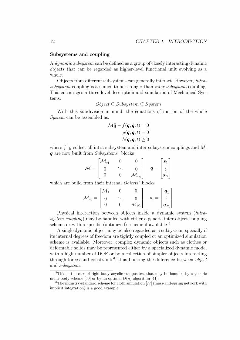
Subsystems and coupling
A dynamic subsystem can be defined as a group of closely interacting dynamicobjects that can be regarded as higher-level functional unit evolving as awhole.
Objects from different subsystems can generally interact. However, intra-subsystem coupling is assumed to be stronger than inter-subsystem coupling.This encourages a three-level description and simulation of Mechanical Sys-tems:
Object ⊆ Subsystem ⊆ System
With this subdivision in mind, the equations of motion of the wholeSystem can be assembled as:
Mq − f(q, q, t) = 0
g(q, q, t) = 0
h(q, q, t) ≥ 0
where f , g collect all intra-subsystem and inter-subsystem couplings and M ,q are now built from Subsystems’ blocks
M =
Ms1 0 0
0. . . 0
0 0 MsN
q =
s1...sN
which are build from their internal Objects’ blocks
Msi =
M1 0 0
0. . . 0
0 0 MNi
si =
q1...
qNi
Physical interaction between objects inside a dynamic system (intra-system coupling) may be handled with either a generic inter-object couplingscheme or with a specific (optimized) scheme if available 5.
A single dynamic object may be also regarded as a subsystem, specially ifits internal degrees of freedom are tightly coupled or an optimized simulationscheme is available. Moreover, complex dynamic objects such as clothes ordeformable solids may be represented either by a specialized dynamic modelwith a high number of DOF or by a collection of simpler objects interactingthrough forces and constraints6, thus blurring the difference between objectand subsystem.
5This is the case of rigid-body acyclic composites, that may be handled by a genericmulti-body scheme [39] or by an optimal O(n) algorithm [41].
6The industry-standard scheme for cloth simulation [77] (mass-and-spring network withimplicit integration) is a good example.

1.2. MOTIVATION 13
Coupling Approaches
There are two main approaches to the problem of simulating a coupled dy-namic system [14]:
• Monolithic: The whole set of coupled subsystems is treated as a singleentity and advanced simultaneously.
• Partitioned: Coupled subsystems are treated in isolation and indepen-dently advanced in time. Interaction is viewed as an inter-subsystemcomunication by means of prediction, substitution and synchronizationat discrete times.
Monolithic Monolithic augmentation symbolically merges the equations ofmotion of all interacting dynamic subsystems and the inter-subsystem cou-pling equations into a single mathematical model. However, systems thatare naturally simulated using different formulations (e.g. Eulerian vs La-grangian), discretizations or algorithms may be very difficult or impossibleto merge.
Monolithic inter-object coupling and inter-subsystem coupling only in-volving objects represented by the same dynamic model (same equations ofmotion) is usually possible and often offers unique optimization possibili-ties due to the uniformity of the equations of motion to be merged7. Forthese reasons monolithic coupling and has been broadly used in interactivesingle-model simulation.
Generic monolithic inter-object and inter-subsystem coupling involvingdifferent dynamic models and different algebraic constraints requires symbol-ically merging any combination of dynamic models and constraints. Naivetreatment of this fact results in a combinatorial explosion of interaction sce-narios that grows intractable 8 if n-way interaction handling is desired.
Optimized monolithic inter-subsystem coupling schemes have been devel-oped for specific situations [11, 8], often yielding good results at the expenseof flexibility and implementation complexity.
7This is exploited in most commercial rigid multibody simulators, for example.8Imagine that we want to simulate an articulated character formed by rigid bodies
that may wear simulated clothes and may drive a simplified car model formed by a rigidbody and deformable rubber weels that can, on extreme impact, explode and break apart.This scenario is not unusual in current-generation racing games. The number of differentdynamic models is 4. If all models were allowed to interact through contact, the numberof different situations would be 24 − 1 (all combinations minus the empty case). Thisproblem is usually overcome by ignoring all non-critical interactions (such as cloth-car,wheel-character, wheel-cloth) at the expense of noticeable visual inaccuracies.

14 CHAPTER 1. INTRODUCTION
Partitioned From a numerical analysis and software engineering point ofview, partitioned treatment of coupled dynamic systems has many advan-tages over the monolithic approach [18]:
• Customization: Each subsystem can be discretized and simulated usingspecialized techniques that are known to perform well in isolation.
• Independent Modeling: Subsystems may be simulated using differentmodels. No symbolic knowledge of other subsystems’ equations of mo-tion is required.
• Software Reuse: Simulation schemes for some subsystems may alreadyexist. The partitioned approach facilitates reusing it in new interactionscenarios.
• Modularity: New methods or implementations may be incrementallyadded without affecting the existing code.
Partitioned methods have been extensively studied by the MechanicalEngineering comunity in relation to structure-structure and fluid-structurecoupled problems. A solid theoretical foundation has been developed andstability and accuracy analysis results are available. Parallel implementationof partitioned simulation has been also studied [16].
Generic partitioned inter-subsystem coupling has been scarcely addressedin interactive dynamics and computer animation research. To our knowledge,only [13] proposed a sound generic algorithm for the simultaneous simulationof coupled dynamics systems with a small overhead.
1.2.2 Interactive Dynamics
Interactive dynamics is a maturing research field with more than two decadesof history. Modern techniques allow the interactive simulation of complexscenes formed by dozens 9 of rigid bodies [67], articulated characters [110],ground and aerial vehicles, clothes [82], ropes and hair [74], and deformablesolids [95]. Interactive simulation of simplified fluids and gases has beenrecently accomplished [103].
Most research works in interactive dynamics to date have focused on asmall set of specific dynamic models that are relevant to their target problemand have developed specifically taylored methods that, while extremely fast,are not easily extended. Inclusion of new dynamic models and their couplingis rarely considered.
9Hardware-accelerated game physics has raised this threshold to thousands.
1.2. MOTIVATION 15
Computer Graphics and Animation
In the production of CG feature films most mechanical models have beensimulated, including particle systems [38], rigids bodies and multibody com-posites [51], elastic, plastic and fracturing deformable solids [85], clothes [77],fluids [102] and smoke [9], as well as other non-mechanical physically-basedspecial effects such as fire and explosions [101]. This field gave birth to theconcept of plausible physics, prioritizing visually pleasing results over physi-cally accurate simulation.
The production of a computer animation sequence is an iterative processin which the animator sets up the virtual scene, animates it using a combi-nation of keyframing, kinematics and dynamics tools, observes the resultinganimation and, if not pleased, changes in the initial setup to improve the re-sults. Control on the final appearance is of foremost importance, and manualad-hoc methods such as artificial force field placement and keyframe post-edition are not uncommon. Therefore, minimization of the setup-animate-observe iteration time is important and encourages the research of fast sim-ulation algorithms that are almost interactive. Some of this techniques havebeen later optimized and used in videogames, which share the weak require-ment of plausible physics with CG, and stable research links between bothfields have emerged.
Multi-model and inter-subsystem interactions have been usually handledas one-way interactions [98], by approximate penalty methods or, in somecases, by speficic two-way interaction algorithms [9]. Generic multi-modelmonolithic coupling has been studied and there is a solid foundation based onthe Lagrange formulation [1]. A generic inter-subsystem partitioned couplingscheme was proposed in [13] with apparently small impact in later researchpublications.
Videogames
Videogames require the execution of several complex subsystems at a highrefresh rate (60Hz) in order to ensure a successful user experience. Each ofthis subsystems (Input processing, Game Logic, Artificial Intelligence, Ani-mation, Graphics and Sound) is assigned a low CPU budget that guaranteesthe execution of all subsystems within a time slice (1/60). Dynamics simula-tion is only a part of the Animation subsystem, and therefore its CPU usageis tightly bounded (tipically 2-3ms per frame). In addition, most videogamesrequire a number of simulataneous objects to be simulated (> 10) to produce

16 CHAPTER 1. INTRODUCTION
the illusion of realism in the game world 10.Given all this limitations, game physics has traditionally focused on sim-
ulating dynamic systems formed by dozens of rigid bodies coupled by contactand mechanical joints [66, 65]. Ideal rigid bodies are simple enough to be ef-ficiently simulated and realistic enough to describe the dynamics of commonobjects found in game worlds. Contact handling guarantees the consistencyof the game world, while mechanical joints allow the simulation of simplifiedmechanisms and articulated characters. This is the standard functionalitysupported by all game-physics middleware [111, 112, 113, 114].
Taking advantage of the increasing CPU power available on domesticcomputers and game consoles, other dynamic models have been successfullysimulated in videogames, such as clothes [82], ropes [74], deformable solids[95], water surfaces and smoke. Recently, the simulation of fluid volumes hasbecame possible by means of hardware acceleration [112].
Game physics is one of the most active research areas in interactive dy-namics. Visual realism, robustness and raw speed are the primary objec-tives of game-specific simulation methods, usually achieved through agres-sive optimizations that sacrify accuracy and generality. Multi-model andinter-subsystem coupling, when considered, is usually limited to one-way in-teractions in a master-slave scheme (e.g. characters wearing dynamic clothesdo not feel the cloth weight and collisions). Some simplified two-way cou-plings have been studied and simulated using pairwise specific algorithms,such as rigid-fluid buoyancy [12].
Virtual Medicine and Haptics
Virtual Medicine applications often involve the interactive exploration ormanipulation of simulated anatomical structures represented as deformablesolids [86]. Though physical accuracy is important, the emphasis is usuallyset in successfully handling detailed user interaction by means of virtual toolsfor touching [86], cutting [96] and suturing [72] the virtual object. Moder-ate simulation refresh rates (>15Hz) are sufficient except when the virtualtools are used through a haptic device, which requires very high simulationfrequency (1000Hz). Virtual medicine applications tend to focus on a small
10When immersed in a graphically realistic game world the player expects virtual objectsto behave in a similarly realistic way. Buildings, terrain and strongly attached objects areassumed to be static. On the other hand, any free medium sized object in the world isexpected to move according to the laws of physics, specially when it interacts with theplayer or other virtual objects (e.g. a chair should move if we push it, a bottle shouldroll, a hanging lamp should oscillate). Failing to meet this expectations in game worldslabeled as ¡real! by the marketing department causes the player’s suspension of disbeliefand dissatisfaction.

1.3. DISCUSSION AND OBJECTIVES 17
region of the anatomy such as a single organ, keeping the simulation com-plexity bounded so that the interactivity requirements can be met [3, 86].In virtual medicine simulations mechanical coupling is usually limited to thetool-structure case.
1.3 Discussion and Objectives
Interactive dynamics has become an important area in many applicationfields. Even though existing techniques enable interactive simulation of mostdynamic models of interest, these rarely deal with multi-model and inter-subsystem coupling. A few efforts have focused on monolithic coupling ofspecific model pairs and monolithic coupling of specific subsystem pairs, butthe practical simulation of all interesting dynamic models and subsystemswith arbitrary coupling in a common virtual environment remains an openproblem.
We believe that generic treatment of multi-model and inter-subsystemcoupling is a necessary step to achieve the interactive simulation of trulyplausible worlds where mechanical interaction between physical objects isnot artificially limited.
The mathematical and computational tools required to solve general cou-pled dynamics problems, modeled as index-3 DAEs, exist and are commonlyused in offline simulation and computer algebra systems (CAS) (see [106]for a historical review). However, general purpose DAE solvers generallyprioritize accuracy over efficiency and involve expensive numerical methods[115]. For these resasons, interactive simulation has traditionally sacrifiedgenericity and physical accuracy in favor of efficiency and stability, usingspecific and strongly simplified mathematical formulations and solvers underthe weak premise of plausible physics.
We feel that the efficiency difficulties could be already overcome thanksto the recent boost in the computational resources available in modern com-puters and gaming consoles (Multicore CPUs, PPU, GPGPU). An effort innumerical analysis and software design and implementation is required inorder cristallize these resources into a generic interactive coupled mechanicalsimulation scheme. A few research efforts in medical simulation, embodiedas open source simulation frameworks, are currently devoted to this task[107, 108].
From a software engineering perspective, the design and implementationof a simulation framework that supports generic coupling efficiently enoughto achieve interactivity is a complex task. The generic mathematical treat-ment of coupled simulation requires a similarly generic/abstract design. In
18 CHAPTER 1. INTRODUCTION
addition, achieving the required efficiency in a generic formulation/designis considerably more difficult, as many specific optimizations implementedby traditional simulation schemes are not possible. However, the numerousadvantages of such a framework (genericity, modularity, extensibility) placeit as a complex but worthy endeavour.
In this work, as a first step towards the development of a mathemati-cal and software framework for interactive simulation of coupled mechanicalsystems, we will analyze the state of the art in interactive simulation ofindividual dynamics models (Chapter 2) and review the existing researchon coupled mechanical systems (Chapter 3). This will allow us to gatherthe requirements and propose a design for a simulation software framework(Chapter 4) that must fulfill two main objectives:
1. Simplify the research, development and comparison of coupled simula-tion schemes in a common environment.
2. Used as an external library, simplify the development of applicationsthat require interactive simulation, such as videogames.
An early prototype of such framework already exists as a personal Open-Source project hosted at http://saphyre.sf.net.

Chapter 2
State of the Art in InteractiveDynamics
In this chapter review the types of mechanical objects that have been sim-ulated at interactive rates, together with the main simulation schemes pur-posed for each one. We are mainly interested in the mathematical formu-lations and numerical algorithms that best simulate each model from anefficiency and robustness perspective.
We will discuss all simulation schemes using common criteria and nota-tion, in order to facilitate comparison and global understanding. For eachreviewed simulation scheme for each model we will detail:
• Equations of motion formulated.
• Numerical methods used.
• Stability and convergence analysis (if available).
• Asymptotic and expected complexity of the computational implemen-tation.
2.1 Particles
A particle is a mass that can only undergo a translation movement throughspace, without rotation or deformation. A particle in R
3 has 3 position DOF:
r =
xyz
19

20 CHAPTER 2. STATE OF THE ART IN INTERACTIVE DYNAMICS
Single particles are the simplest dynamics objects, and have been tradi-tionally used in interactive simulation to model small objects (e.g. debris,projectiles).
The equations of motion of a free particle are:
mr − f(r, r, t) = 0
Or first order ODE form:[r
p
]=
[1mp
f
]
where m is mass, f is force and p = mr is the linear momentum.
2.1.1 Particle Systems
Particle systems were introduced to the Computer Graphics community in[38] to simulate heterogeous phenomena (e.g. debris, explosions, sparks,engine trails, fire, smoke, dust, water streams...) that can be approximatedby a collection of non-interacting point-masses guided by simple dynamicsrules.
In a general particle system, particles can interact through inter-particleforces and constraints. The equations of motion of a system of N particleswith inter-particle force interactions can be written in block form:
Mq − f(q, q, t) = 0
with
M =
m1I3 0 0
0. . . 0
0 0 mNI3
q =
r1...rN
f(q, q, t) =
f1(q, q, t)
...fN(q, q, t)
where I3 is the 3 × 3 identity matrix, q gathers the configuration ri of allparticles i = 1..N and f gathers all external and inter-particle forces of thesystem.
Inter-particle forces may have any expression but should obey the action-reaction principle in order to preserve momentum. The most common inter-particle force used in interactive simulation is a spring, usually formalized asa Hookean elastic force with linear damping [71]:
fij = Ks
(Lij − 1)
‖ri − rj‖(ri − rj)−Kd
(ri − rj)T (ri − rj)
‖ri − rj‖2(ri − rj)

2.1. PARTICLES 21
where Ks and Kd are the elasticity and damping coefficients, and Lij is thespring’s rest-length.
Exact algebraic constraints may be defined on a particle system by aug-mentation of the equations of motion, yielding a DAE:
Mq − f(q, q, t) = 0
g(q, q, t) = 0
h(q, q, t) > 0
From a reductionist perspective, any mechanical object can be approx-imated by a set of particles that interact through contact, constraints andinter-particle forces. This has been widely exploited in interactive simulation,and several complex models are traditionally simulated as mass and springnetworks, constrained particle systems or hybrid spring-constraint models.
Mass and Spring Networks
Mass and spring networks can represent any deformable objects (curves, sur-faces and solids) assuming that the material properties can be approximatedby elastic damped forces between neighbour particles that discretize the ob-ject’s mass.
Generic inter-particle elastic forces may be generated from energy con-straints [6, 88], which are potential energies that depend on particles’ posi-tions and are minimized when the constraint is fulfilled:
C(r1, . . . , rN) = 0 the constraint
E(r1, . . . , rN) =1
2KsC
2 the energy
fCi (r1, . . . , rN) = −
∂E
∂ri
the force
= −Ks
∂C
∂ri
C
Damping can be added to an energy constraint force, yielding:
fCi (r1, . . . , rN ; r1, . . . , rN) = −Ks
∂C
∂ri
C −Kd
∂C
∂ri
C
Energy constraints are not exactly fulfilled in presence of external forcesor in overconstrained systems, but their minimization nature ensures a goodsolution in situations where an exact solution is not possible. Energy con-straints behave as generalized springs, and are closely related to the penalty

22 CHAPTER 2. STATE OF THE ART IN INTERACTIVE DYNAMICS
method. Constraints can be made arbitrarily stiff by increasing the Ks pa-rameter, thus reducing constraint violation at the cost of complicating thenumerical solution, which requires implicit integration to ensure stability.Cloth simulation has extensively used mass and spring networks [77], seesection 2.4 for a detailed discussion.
Constrained particle systems
A particle-based simulation scheme for deformable objects strictly focusedon stability and efficiency was introduced to the game physics community byJakobsen in [79]. The scheme is similar to a mass and spring network wherethe inter-particle elastic forces that model the structure of the deformableobject are substituted by fixed distance constraints, that can be interpretedas massles rigid rods connecting pairs of particles. This kind of model willbe named constrained particle system through this work.
Instead of deriving an inter-particle constraint force that maintains theconstraint during time-integration of the equations of motion, Jakobsen’s ap-proach starts with an unconstrained step in which particles are independentlyintegrated accounting for external forces, followed by a correction step thatdirectly changes particles’ positions until they fulfill the constraints below anerror threshold:
1. Unconstrained integration: Uses a velocity-less Verlet scheme that,while widely used in molecular dynamics, was almost unknown (orat least ignored) to the videogame and computer graphics research co-munities. The main advantage of this integration scheme, apart frombeing symplectic and second order accurate when external forces arevelocity-independent, is that it does not explicitly store or use veloci-ties.
rk+1 = 2rk − rk−1 + h2rk
2. Position correction: Iterative Gauss-Seidel relaxation process that cor-rects each constraint individually in a global loop which is repeated un-til an error threshold (or a maximum number of iterations) is met. Foreach constraint the particle positions are displaced along the constraintgradient direction in order to eliminate constraint violation. Particlesare displaced proportionally to their inverse masses. Jakobsen identifiesthis correction scheme as an interior point method.
For example, a constraint on a pair of particles (i, j) that keeps them
2.2. RIGID BODIES 23
at a fixed distance Lij can be formulated as:
C(ri, rj) = ‖ri − rj‖ − Lij = 0
∇C =1
‖ri − rj‖
[(ri − rj)−(ri − rj)
]T
Defining d = (ri − rj) and d = d‖d‖
, the correction on each particle is:
r+i = r−
i +mi
mi +mj
(Lij − ‖d‖
)d
r+j = r−
j −mj
mi +mj
(Lij − ‖d‖
)d
The key idea in Jakobsen’s scheme is that direct particle position correc-tion simultaneously corrects particle velocities, as they are implicitly definedby rk − rk−1. This makes the method very efficient and stable/robust, asvelocities are always bounded.
Individual constraint correction can be enforced exactly or with an under-relaxation coefficient Ku ∈ (0, 1] that may improve convergence and allowsfor interesting effects such as soft bodies. Constraint underrelaxation to sim-ulate the material properties of elastic-plastic bodies has been studied in [82],where a method to decouple the underrelaxation coefficient from the numberof global relaxation iterations is introduced. This approach to deformablemodeling is very fast and robust, but does not have a physically-based the-oretical background, and the underrelaxation parameters are not directlyrelated to physical material coefficients.
The constrained particle system model as introduced by Jakobsen [79]and extended in [82] has been successfully applied to objects such as clothes,ropes and deformable solids as well as rigid objects represented as 4 particleswith distance constraints forming a tetrahedron, and is inmensely popular inthe videogame field due to its simplicity, efficiency and robustness1.
2.2 Rigid Bodies
A rigid body is an idealized object cannot be deformed and therefore mayonly undergo rigid motion: translation and rotation. Rigid bodies allow
1Although Jakobsen published this method in 2001, a game-physics middleware andhardware company claimed and was granted a US patent describing an extremely similarmethod in 2005, a fact that furtherly demonstrates that we are doomed to live in a“civilization” ruled by mindless capitalism instead of ethics or common sense.

24 CHAPTER 2. STATE OF THE ART IN INTERACTIVE DYNAMICS
the representation of solids with only 6 DOF, thus being very compact andefficient to simulate as opposed to deformable objects, which require a highnumber of DOF. The configuration of a rigid body in R
3 has 3 DOF for theposition of the CoM (Center of Mass) and 3 DOF for the orientation, andcan be mathematically represented as:
qeuler =
[r
θ
]qmatrix =
[r
R
]qquaternion =
[r
Q
]
where the position DOF representation is common
r =
xyz
but the orientation DOF representation is either a set of 3 euler angles θ, a3× 3 rotation matrix R or a unit quaternion Q:
θ =
θxθyθz
R =
R0,0 R0,1 R0,2
R1,0 R1,1 R1,2
R2,0 R2,1 R2,2
Q =
Qx
Qy
Qz
Qw
A discussion on the benefits and drawbacks of each orientation represen-tation is out of scope and can be found elsewhere. We will stick to the unitquaternion representation as it’s widely proven to avoid singularities whilebeing compact (4 real values instead of 9 in case of a rotation matrix). Con-version between rotation matrix and quaternion representations is alwayspossible and will be used for convenience.
The Newton-Euler equations of motion of a free rigid body in world co-ordinates are:
mr − f(q, q, t) = 0
Iω −L× ω − τ(q, q, t) = 0
where the first equation determines the evolution of the translational DOFand is the same as with particles, and the second equation determines theevolution of the rotational DOF and introduces several new concepts2:
I is the inertia tensor around the CoM
2Full derivation of the equations of motion of a rigid body can be found in any classicalmechanics text such as [40].

2.2. RIGID BODIES 25
The inertia tensor is a symmetric positive definite 3 × 3 matrix thatrepresents the rotational mass properties of the rigid body.
I = RIbodyRT
where R(Q) is the instantaneous orientation of the rigid body andIbody is the constant inertia tensor with respect to the rigid body localreference frame.
ω is the angular velocity around the CoM
Angular velocity is a vector in R3 whose direction determines the in-
stantaneous axis of rotation and whose length determines the instan-taneous rotation speed around this axis.
τ is the torque around the CoM
Torque is the angular effect of a force f applied to a point rf on therigid body.
τ = (rf − r)× f
L is the angular momentum around the CoM
Angular momentum is conserved in absence of net external torque act-ing on the rigid body.
L = Iω
The second order equations of rigid body dynamics can be written morecompactly in matrix form.
We start by defining the generalized velocity vector v (also called twist)and its derivative3:
v =
[r
ω
]v =
[1mf
I−1 (L× ω + τ )
]
the external F e and inertia F inrt generalized forces (also called wrenches):
F e =
[f e
τ e
]F inrt =
[0
L× ω
]
and the 6× 6 mass matrix M and its inverse:
M =
[mI3 00 I
]M−1 =
[1mI3 00 I−1
]
3The derivation of ω can be found in [5] p186.

26 CHAPTER 2. STATE OF THE ART IN INTERACTIVE DYNAMICS
We can now write the matrix equations of motion for a free rigid bodyas:
Mv − F inrt − F e = 0
q = Dqv(Q)v
where the linear relationship between the cofiguration derivative q and thevelocity vector v is made explicit [55, 43]:
q =
[r
Q
]q =
[r
12ωQ
]Dq
v(Q) =
I3 0
0 12
−Qx −Qy −Qz
Qw Qz −Qy
−Qz Qw Qx
Qy −Qx Qw
The equations of motion can be rearranged as a first order system ofODE:
r
Q
p
L
=
1mp
12ωQ
f
τ
where p = mr is the linear momentum of the CoM and ω is convenientlyinterpreted as the pure imaginary quaternion (ω, 0) when multiplied by Q.
2.3 Rigid Multibody Systems
Rigid multibody composites are central to the simulation of mechanismsin robotics, engineering and virtual reality. Rigid bodies can be attachedthrough mechanical joints to build mechanisms, vehicles and articulated char-acters, among others. This versatility, together with their compact DOFrepresentation, make rigid multibodies suitable for interactive simulation.
The equations of motion of a system of N rigid bodies with inter-objectforce interactions can be written in block form:
Mv − F inrt − F e = 0
qi = Dqv(Qi)vi
with
M =
M1 0 0
0. . . 0
0 0 MN
q =
q1...qN
v =
v1...
vN
F e =
F e
1(q,v, t)...
F eN(q,v, t)
2.3. RIGID MULTIBODY SYSTEMS 27
where F inrt collects all inertia forces and F e gathers all external and inter-object generalized forces of the system.
2.3.1 Collision and Contact
Realistic simulation of rigid bodies requires the detection and treatment ofinter-object collision and contact with friction. The rigid body assumptionrequires an instantaneous change of velocity when rigid bodies collide toavoid interpenetration, which introduces a discontinuity in the second orderequations of motion formalized as impulsive forces [46]. Moreover, addingdry Coulomb friction to the equations of motion has been shown to lead toinconsistency and indeterminacy problems [50] in force-acceleration basedformulations.
Most research on rigid multibodies has focused on the frictional colli-sion/contact problem, and although several practical approaches exist [70],the interactive simulation of hundreds of rigid bodies with mechanical jointsand true Coulomb dry friction is still not possible. Current algorithms arebased on simplifications that sacrify friction and constraint accuracy in orderto guarantee efficiency and robustness.
We will now review the three main approaches to collision and contactresolution: penalty methods, analytical methods and propagation methods,and analyze the main contributions to each.
Penalty Methods
First attempts to solve the rigid body frictionless contact problem tried toprevent interpenetration by adding spring and damper elements at each con-tact point that applied a repulsive force to prevent further penetration. Thisapproach, known as the penalty method, is fundamentally flawed as shown byBaraff [49], as it never eliminates interpenetration. This is specially criticalin stacking configurations. Moreover, keeping interpenetration small requiresa large spring elasticity constant, which yields stiff equations of motion thatmust be solved using implicit integration in order to guarantee stability. Inaddition, it is not clear how dry friction can be added in the penalty methodframework [51].
Propagation methods
Pioneered by Hahn [44] and Moore and Wilhelms [45], the propagationmethod was the first practical approach to interactive rigid multibody colli-sion treatment. Collisions are detected and processed one by one in chrono-

28 CHAPTER 2. STATE OF THE ART IN INTERACTIVE DYNAMICS
logical order, and their effect is instantaneously propagated to other bodiesin contact in an recursive/iterative fashion. Due to their pairwaise nature,propagation methods suffered from stagnation (very small timesteps) in rest-ing contact and simultaneous contact situations such as rigid body stacking.
Pairwise collision resolution is generally achieved by means of impulses,that instantaneously change bodies’ velocities to avoid interpenetration whileconserving total momentum and energy in non-dissipative collisions. For thisreason, propagation methods are also called Impulse-based methods.
Given a contact point rc between two rigid bodies A and B, we definerac = rc − ra and ra
c = ra +ωa × rac , and analogously for rb
c, rbc. The relative
collision velocity is rabc = ra
c − rbc. The change of relative collision velocity
induced by an impulse response jc applied at the collision point on each body(jc on ra
c and −jc on rbc) is:
∆rabc = Kjc (2.1)
where K is the nonsingular, symmetric and positive definite collision matrix∈ R
3×3:
K =
(1
ma
+1
mb
)I3 −
(racI
−1a ra
c + rbcI
−1b rb
c
)
where r denotes the cross product matrix of vector r:
r =
0 −rz ryrz 0 −rx−ry rx 0
While this formulation is useful in analyzing frictional collisions, Equation(2.1) can be projected onto the collision normal direction nc to yield a singlescalar equation for the normal collision impulse jc = λcnc.
nTc ∆rab
c = nTc (Kλcnc)
∆rnc = (nTc Knc)λc
∆v = Knλc
Using this projection and denoting pre-collision normal velocity v− andpost-collision normal velocity as v+, a range of frictionless collision responsebehaviours from purely inelastic to purely elastic can be modeled as:
v+ = −ev−
v+ − v− = Knλc

2.3. RIGID MULTIBODY SYSTEMS 29
where e ∈ [0, 1] is the restitution coefficient, and λc can be easily isolated inorder to calculate the normal collision impulse, which will dissipate a fraction(1− e) of the pre-collision kinematic energy.
Impulse-based simulation was popularized by Mirtich [46], who extendedthe method to successfully handle contacts and friction in the impulse frame-work. Moreover, Mirtich’s impulse-based method also incorporated rigidjoints by extending Featherstone’s work [41]. To adress the inherent inef-ficiency of the propagation approach in presence of simultaneous or veryfrequent collisions, a timewarp algorithm was presented in [47], based in es-timating an upper bound on the velocity of each body and asynchronouslyevolving disjoint groups of colliding bodies, which needed to be synchronizedonly when inter-group collisions were possible according to velocity bounds.The impulse-based framework was elegantly formulated as an impulse-graphstructure in [48], which allows a global solution of the impulse propagationprocess.
Despite these contributions, the propagation based approach was not verypopular in the interactive simulation domain due to its unpredictable cost inpresence of frequent collisions. Chronologic collision detection and processingis required to obtain realistic simulations of systems such as Newton’s cradle,but may be too restrictive in interactive simulations, where the amount ofcomputational work per frame is tightly bounded.
In order to overcome the propagation method drawbacks while preservingits simplicity, Guendelman [63] presented a new impulse-based scheme thatallowed efficient collision and contact treatment with stable stacking. Thescheme is based in an impulse-graph structure which is sorted according tostack levels. The stack level of an object is defined as the minimum topo-logical distance to an static object in the impulse-graph. Propagation chainsfollow the stacking order from bottom to top, dramatically accelerating con-vergence. A shock-propagation pass through the graph, where lower levelobjects are considered static when propagating impulses to higher level ones,furtherly improves convergence while being unrealistic. In order to avoidsmall timesteps, the method tolerates and resolves small interpenetrationsin a successive under-relaxation (SUR) fashion, sweeping the contact-graphseveral times and gradually separating overlapping objects. The number ofgraph sweep iterations for each phase can be increased or decreased as atradeoff between accuracy and computation time.
Guendelman’s scheme resurrected the interest in propagation methodsin the interactive domain and has been extended by Weinstein [66] to in-corporate rigid multibody equality constraints. Weinstein introduced a pre-stabilization scheme that uses fixed-point Newton-Raphson iteration to solvea small nonlinear problem for each joint that avoids most constraint error in

30 CHAPTER 2. STATE OF THE ART IN INTERACTIVE DYNAMICS
the next frame. The joint-local process is embedded in the global propagationalgorithm of Guendelman together with contact treatment. Weinstein alsouses SUR to stabilize constraint positional errors to improve visual quality.
The work of Bender and Schmitt [67, 68, 69] is based in a pre-stabilizationscheme like Weinstein’s, but where nonlinear joint/constraint functions arelinearized in order to allow a global solution formulated as a system of linearequations (SLE). This is shown to converge much faster as the number ofobjects and constraints increases. Constraint cycles are detected and decou-pled following Faure’s [54] approach and each constraint graph partition isefficiently solved in linear time using Baraff’s factorization algorithm [53].Multiple contacts per body are treated with a body-local iterative process[67] that also allows faster convergence than global propagation of individualcontact responses.
Kaufman [64] presented a multibody contact scheme that solves per-bodysimultaneous contacts in the each body’s generalized velocity configurationspace. For each body, the constraint manifold in generalized velocity spaceis approximated and a feasible wrench/twist is computed by projection ontothe convex feasible region. The twist projection requires solving a convexquadratic program (QP) that can be approximated with an algorithm linearin the number of contacts per body, yielding a method that is linear inthe number of total contacts while handling per-body simultaneous contactsrobustly. Reported running times are promising, though interactivity wasnot an objective4.
Propagation methods are commonly compared to and identified as Gauss-Seidel processes in literature, thus suffering from low convergence rate whenpropagation chains are long and in presence of cycles. However, recent im-provements of the propagation process by means of contact-graphs, shock-propagation, robust treatment of interpenetrations and analytic computationof impulses in densely constrained configurations have evolved it into a ma-ture and practical constrained multibody scheme that has been shown torival analytical methods in both efficiency and stability.
Analytical methods
In a series of articles during the late 80’s and early 90’s Baraff [49, 50, 51, 52]presented analytical methods aimed to computing the exact contact forcesthat would generate zero-penetration (as opposed to the penalty method)and would not suffer from stagnation problems due to simultaneous contacts
4The chosen implementation language, Java, is not regarded as fast in the interactivesimulation domain. This is specially true in videogames, where optimized implementationsare usually written in C++ with critical parts in assembler.

2.3. RIGID MULTIBODY SYSTEMS 31
(as opposed to propagation methods). His approach, based on previous workby Lotstedt [42], involved solving a Linear Complementarity Problem (LCP)[116], which was proven to have a solution for frictionless contacts, but notfor contacts with Coulomb friction. In a configuration with n contact pointswe define a = Af + b with A ∈ R
n×n and a,f , b ∈ Rn, where ai is the
normal acceleration at contact point i, fi is the normal force multiplier atcontact point i, b reflects external and inertia forces, and A is a matrix thatreflects masses and contact geometries of the bodies. The LCP formulatedby Baraff is:
Af + b > 0 (2.2)
f > 0 (2.3)
fT (Af + b) = 0 (2.4)
Equation (2.2) states that normal accelerations must be nonnegative, pre-venting interpenetration. Equation (2.3) states that normal forces must benonnegative, thus not not opposing separation. Equation (2.4) is the com-plementarity condition and must be understood component-wise fiai = 0,and states that either the contact normal force or the normal accelerationat a contact point must vanish, preventing contact forces from acceleratingcontacts apart.
The Coulomb friction conditions for each contact point are:{f 2x + f 2
y ≤ (µfn)2 and (fx, fy)
T (ax, ay) ≤ 0 if (vx, vy) = 0
(fx, fy) = −µfn(vx,vy)
‖(vx,vy)‖if (vx, vy) 6= 0
(2.5)
These conditions introduce a nonlinear coupling between normal contactforce fn and tangential friction force (fx, fy). Due to this coupling, the prob-lem is no longer an LCP but an NLCP (Nonlinear Complementarity Prob-lem). Geometrically, Coulomb friction defines a friction cone that containsany feasible (fx, fy, fn). The friction cone can be approximated by an n-sidepyramid, which restores linearity and enables an LCP formulation.
Other force-acceleration based schemes have been proposed, but none canbe guaranteed to yield consistent results during transitions between kine-matic and static friction, as force discontinuities appear that lead to infiniteinstantaneous accelerations. These discontinuities will break the numericalintegration unless they are detected and resolved using impulses instead offorces. Baraff [49] modified the LCP solver to detect such situations andswitch to an impulse-based formulation, but the method is cumbersome andnot guaranteed to work in real-world simulations.
The first solvable rigid body contact scheme was presented by Anitescuand Potra in [59] based on previous work by Pang, Stewart and Trinkle.

32 CHAPTER 2. STATE OF THE ART IN INTERACTIVE DYNAMICS
The scheme, based on the impulse-velocity formulation with a linear frictionpyramid, was demonstrated to be solvable by Lemke’s LCP algorithm forany number of contacts and any nonnegative friction coefficient. In addition,equality constraints in the form g(q,v, t) = 0 can be easily accomodated,yielding a Mixed-LCP (MLCP). The MLCP formulated by Anitescu-Potrais:
M(vk+1 − vk) = J Tg λg +
p∑
i=1
(nifni+Diβi) + hF (2.6)
Jgvk+1 = 0 (2.7)
ρi = nTi v
k+1> 0 compl. to fni
> 0, i = 1 . . . p (2.8)
σi = λiei +DTi v
k+1> 0 compl. to βi > 0, i = 1 . . . p (2.9)
ζi = µifni− eT
i βi > 0 compl. to λi > 0, i = 1 . . . p (2.10)
Equation (2.6) is a first order time-stepping formula for a rigid bodysystem with timestep h, where vk is the generalized velocity at step k, Jg
is the jacobian of the equality constraints g, λg is the vector of lagrangemultipliers for the equality constraints, p is the number of contacts, ni is thenormal at contact i, fni
is the normal contact impulse at contact i, Diβi isthe tangential friction impulse at contact i, and F = F inrt + F e are inertiaand external forces on the system.
Equation (2.7) is the differentiated equality constraint condition andstates that legal velocities must be perpendicular to the constraint gradi-ent.
Equation (2.8) is the contact normal condition, which restricts legal ve-locities to be perpendicular to the normal and complementary to the normalimpulse fn. This formulation of the nonpenetration constraint is the keycontribution of Anitescu-Potra that guarantees solvability in nondegenerateconfigurations.
Equations (2.9) and (2.10) are the friction force complementarity condi-tions corresponding to a friction pyramid approximation to the friction coneat each contact:
FC(q) = {nfn +Dβ | fn > 0, β > 0, eTβ > µfn} (2.11)
where D ∈ R3×u is a non-orthogonal basis matrix formed by u column vectors
dj that represent the space tangent to the contact, β ∈ Ru is the vector of
impulse multipliers in each direction dj and e = [1, . . . , 1]T ∈ Ru.

2.3. RIGID MULTIBODY SYSTEMS 33
The MLCP (2.6)-(2.10) can be written in matrix form:
M −Jg −N −D 0J T
g 0 0 0 0N T 0 0 0 0DT 0 0 0 E0 0 µ −ET 0
vk+1
λg
fn
β
λ
+
−Mvk − hF0000
=
00ρ
σ
ζ
(2.12)fn
β
λ
T ρ
σ
ζ
= 0
fn
β
λ
> 0
ρ
σ
ζ
> 0 (2.13)
where N is the matrix formed by all contact normals ni, D is the matrixformed by all contact conesDi, E = diag(e1, . . . , ep) and µ = diag(µ1, . . . , µp).
Several improvements over the initial Anitescu-Potra formulation havebeen presented, including contact normal nonlinearity handling by fixed pointiteration [58], implicit time-stepping for stiff systems [60], partitioned sys-tem solving by Block-MLCP [70], and a regularized formulation that en-sures solvability in degenerate configurations [115]. An iterative algorithmby Anitescu-Tasora [61] has been recently presented and shows promisingresults in solving frictional contacts for thousands of objects.
A few simplifications of the friction cone have been investigated: (i) De-coupling tangential and normal contact forces through splitting (normal-tangential force interleaving and (ii) Linearizing the quadratic term witha polygonal approximation (friction pyramid). Both simplifications lead tosmaller/simpler problems that can be solved more efficiently at the cost ofrealism and friction anisotropy respectively. Approaches can be combinedto yield cylindric friction (split,nonlinear), box friction (split,linear) (widelyused in videogames), and the previously explained pyramid friction (cou-pled,linear).
Known LCP solvers have an exponential asymptotic complexity on thenumber of contacts O(2nc) and expected polynomial complexity, thereforethey may be prohibitively expensive in highly packed configurations wherethe number of contacts per object is expected to be high. In this situations,more efficient position-based optimization methods have been presented [62].Optimization Based Animation (OBA) requires the solution of quadratic min-imization problems (QP) on the object’s configurations, and velocities, noton the contact forces or impulses.
An iterative game-oriented algorithm for the approximate solution of theMLCP arising in multibody simulations with contacts and constraints waspresented in [65]. The algorithm uses box-friction and allows early exit of the

34 CHAPTER 2. STATE OF THE ART IN INTERACTIVE DYNAMICS
iteration process, based in the projected gauss-seidel (PGS) algorithm. Whilebeing very inaccurate, the method is well suited for videogames. This methodwas formally shown to be equivalent to the sequential impulse propagationmethod, thus establishing a connection between analytic and propagationmethods.
Discussion
In Table 2.3.1 we summarize the mathematical and computational details ofthe most relevant contributions to the interactive simulation of rigid multi-bodies with frictional contact we’ve reviewed so far.
Fml Friction Step Stab Math NM Cost
Penalty F ∅ Im ∅ SLE CG O(nc)
Bar94 [52] F Cone Ex Bau LCP Dantzig O(2nc)
AP97 [59] V Pyr FE Proj MLCP Lemke O(2nc)
Sch02 [62] P Pyr Ex QP QP IPM O(n2cb)
Cat05 [65] I Box SIE Bau MLCP PGS O(knc)
Lac07 [115] V Pyr Im GP-RD MLCP Lemke O(2nc)
Mir00 [47] I Cone Ex ∅ ∅ O(knc)
Gue03 [63] I Cone FE SUR ∅ O(knc)
Kau04 [64] I Cone V ∅? QP SCM O(nb + nc)
Wei06 [66] I Cone FE Pre/SUR SNE NR O(knc)
Ben06 [69] I Cone FE/Ex Pre SLE LDL O(knc)
Fml : Mechanical problem unknowns { F: Force, V: Velocity, I: Impulse, P: Position }
Friction : Friction model {Cone, Pyr: Pyramid, Box}. S: Split normal force, decoupled from friction force.
Solvable : Solvability/Convergence proof available? { Yes, No }
Step : Integration step type {Im: Implicit (any), Ex: Explicit (any), SIE Semi Implicit Euler, FE: Forward Euler, V:Verlet, RK: Runge-Kutta}.
Stab : Stabilization method {Pre: Pre-Stabilization, Proj: Post-Projection, Bau: Baumgarte, SUR Successive Under-Relaxation, GP-RD: Ghost Potential - Rayleigh Dissipation (see [115])}.
Math : Mathematical problem formulated { SLE: System of Linear Equations, SNE: System of Nonlinear Equations,LCP: Linear Complementarity Problem, MLCP: Mixed LCP, QP: Quadratic Program }.
NM : Numerical methods involved { CG Conjugate Gradient, Dantzig LCP, Lemke LCP, PGS Projected Gauss-Seidel,
SCM Surrogate Constraint Method, IPM Interior Point Method, NR: Newton-Raphson, LDL: LDLT matrixfactorization }.
Cost : Asymptotic complexity (worst case) per simulation step. nc is the number of contacts and constraints. nb isthe number of bodies. ncb is the number of close body pairs. k is a user-tunable constant, usually an iterationcount.
Table 2.1: Multibody Contact Approaches.
Analytic methods have attracted most research attention in Robotics andComputer Graphics literature, as they have a solid theoretical foundation

2.4. CLOTHES 35
and convergence results. Moreover, widely used game-oriented commercialrigid multibody simulation middleware is reported to use analytical methods.However, the worst case complexity of MLCP solvers and their optimizationdifficulty set an upper bound of hundreds on the number of bodies/contactsthat can be interactively simulated.
On the other hand, novel propagation methods presented by Guendelman[63] and others [66, 69] have dramatically reduced the traditional drawbacksof such methods while keeping their worst case complexity linear in thenumber of contacts, and include a few parameters (e.g. subprocess iterationcounts) that can be used to achieve the desired tradeoff between accuracyand running time while preserving stability.
We feel that propagation methods, while less elegant and mathematicallysound than analytic methods, have numerous advantages in interactive sim-ulation (asymptotic complexity, easier to implement and optimize, accuracy-speed tradeoff parameters, robustness) that will continue increasing theirpopularity. In fact, first class contributors to the develompent of analyticmethods such as Anitescu are lately researching iterative algorithms to solveMLCPs [61] that are closely related to propagation methods.
As a closing remark, propagation methods can be theoretically connectedto the partitioned approach to the simulation of coupled mechanical sys-tems in which we are mainly interested. Similarly, analytic methods can beconnected to the monolithic approach to coupled systems.
2.4 Clothes
The Computer Graphics community became soon interested in cloth simula-tion in order to automatically predict the stable configuration or the dynamicmotion of common-life objects such as curtains, tabletops, flags, or charac-ter clothes in animated feature films and commercials. Real clothes exhibitvery complex behaviours (including self-collisions, folding, wrinkling, shear-ing, tearing and air friction) that are tremendously expensive to animate byhand. First cloth simulation algorithms appeared in the late 80’s [85], butfast and robust production-level simulation schemes were not available untilmid 90’s.
Interactive cloth simulation adapts offline simulation schemes and is gen-erally optimized for coarser cloth discretizations, ignoring most expensiveaspects such as self-collisions and tearing. Cloth simulation is a common fea-ture in current generation videogames, as it contributes to the realism andspectacularity of game worlds at a reasonable cost.

36 CHAPTER 2. STATE OF THE ART IN INTERACTIVE DYNAMICS
2.4.1 Mass and Spring Networks
The most popular approach to cloth simulation is representing the clothsurface as a mass and spring network. Inter-particle forces in a cloth sur-face (stretch, shear and bending) can be modeled as energy constraints asdescribed in Section 2.1.1. Real clothes exhibit moderate shear and bend-ing resistance but very strong stretch resistance due to their internal wovenstructure. Simulating such a strong resistance as an elastic damped forcerequires a high elasticitiy constant that results in a stiff system. Numericalintegration of stiff systems is ill posed and requires very high order-accuracyintegrators (RK4) and small or adaptative timesteps to guarantee stability,which is computationally expensive.
In this context, Baraff and Witkin [77] introduced a widely used methodfor simulating mass and spring network clothes with first order implicit inte-gration (Backwards Euler) that allows for moderately large timesteps whilepreserving stability. Their method became a de facto standard, despite itsartificial energy dissipation and inaccuracy. Collecting the positions of all nparticles in the configuration vector q we can write the equations of motionof the particle system as:
Mq − f(q, q) = 0
We transform it into a first order system defining:
y =
[q
q
]
y =
[q
M−1f(q, q)
]= F (y)
Discretizing the first order equations of motion using a Backwards Euler(implicit) scheme we obtain:
yk+1 = yk + hF (yk+1)
∆y = hF (yk+1)
where F (yk+1) can be aproximated by a first order Taylor expansion aroundyk as:
F (yk +∆y) = F (yk) +∂F
∂y∆y
plugging it into the BE step:
∆y = h
(F (yk) +
∂F
∂y∆y
)

2.4. CLOTHES 37
and expanding y:
[∆q
∆q
]= h
[qk +∆q
f(qk, qk) + ∂f
∂q∆q + ∂f
∂q∆q
]
Finally, we substitute the first equation into the second, yielding:
(I− hM−1∂f
∂q− h2M−1∂f
∂q
)∆q = hM−1
(f(qk, qk) + h
∂f
∂qqk
)(2.14)
which can be seen as a system of 3n linear equations A∆q = b. This SLE canbe solved for ∆q, which can be later used to calculate ∆q. Matrix A is verysparse because each particle only interacts directly with its neighbours. Inaddition, due to some simplifications A is Symmetric and Positive Definite(SPD) and can be efficiently solved with the Conjugate Gradient method.The CG solver is modified in order to embed per-particle constraints directlyon the search directions, without the need of Lagrange multipliers or penaltyforces. Cloth self-collision is treated by stiff repulsion forces that are robustlyintegrated thanks to the implicit BE method.
The linearized implicit formulation of Baraff and Witkin [77] can be op-timized if stiff and non-stiff elastic damped forces are decoupled. Whilestiff stretch forces require implicit integration for stability, nonstiff shear andbending forces may be integrated explicitly, reducing the inter-particle cou-pling in equation (2.14) and thus increasing the sparsity of matrix A. This isknown as the IMEX scheme [78]. A method to automatically decide whichinter-particle forces should be treated explicitly and which implicitly accord-ing to an instantaneous stability criterion was presented in [81]. Cloth areasthat are only coupled by instantaneously nonstiff force connections can besolved independently regarding the stiff forces.
Cloth tearing can be easily handled in mass and spring networks byremoving the teared inter-particle connections, thus changing the networktopology, which may allow for further decoupling. A physically based maxi-mum strain criteria can be used to decide which springs should break.
2.4.2 Constrained particle systems
The constrained particle system formulation described in Section 2.1.1 issuitable to model clothes. Stretch is represented as inter-particle hard lengthconstraints, while shear and bending resistance are represented as underre-laxated length constraints.
Per particle external constraints such as moving attachment points areeasily integrated in the constrained particle system approach, as positions

38 CHAPTER 2. STATE OF THE ART IN INTERACTIVE DYNAMICS
may be directly changed to fulfill external constraints exactly in a single step.However, clothes attached to fast moving characters require special consid-eration, as the constraint relaxation process may require a large amountof iterations to converge, thus becoming expensive. In cloth and hair sim-ulation system implemented by the author for an unpublished videogame(Soccer Fury) this problem was solved with the addition of a per particleconstraint relaxation factor in the range ∈ [0, 1] that was used to bias thecorrection process so that particles topologically closer to the cloth-characterattachment points were displaced less than farther ones. This is similar toincreasing/decreasing individual particle masses but only affects constraintcorrection, not unconstrained integration inertia.
Tearing can be included in the constrained particle system formulation byremoving broken connections, but a physically based criterion to decide whichconnections should break due to external stress is not easy to find, as inter-particle forces are never computed explicitly. However, heuristic approachesbased on inter-particle distance can yield plausible results as shown in [82].
2.4.3 Hybrid approaches
A recent contribution to cloth simulation [83] uses an hybrid approach inwhich stretch is modeled as an equality constraint (fixed inter-particle dis-tance) while shear and bending are modeled as elastic damped forces andintegrated explicitly using a Forward Euler scheme. At each timestep themethod performs a forward unconstrained step with explicit forces followedby a correction phase in which particles’ configurations are projected on tothe constraint manifold along the constraint gradients evaluated at the nexttimestep. This involves solving a sparse and SPD system of n linear equa-tions (three times smaller than the ones solved for the implicit and the IMEXschemes), as the unknowns are the gradient scalar multipliers, not R3 veloc-ities. The projection phase is iterated until a certain upper bound on themaximum strain generated by elastic forces is met. Particle velocities arerecomputed from previous and current positions after projection. Stabilityresults are not provided.
Personal experience in the implementation of a very similar hybrid methodshowed that either small timesteps, small shear/bending elasticity coefficientsor several projection iterations are required to ensure stability when clothesare attached to fast moving characters. Therefore the hybrid method, whichperforms well in its target application (offline simulation), was discarded forinteractive simulation in favor of the previously described constrained particlesystem formulation with soft shear and bending underrelaxation coefficients.

2.5. CURVES 39
2.5 Curves
Thin deformable objects representing ropes, wires, cables, surgical threads,hair and plant trunks have been successfully simulated at interactive rates.This kind of objects can be approximated as thin axially-symmetric tridimen-sional curves with an arc-length parametrization r(s), which allows formu-lating and solving the dynamics model on an unidimensional discretizationalong parameter s. This results in mathematical models with a moderatenumber of DOF, much smaller than clothes or deformable solids, and there-fore suitable to be interactively simulated.
Three approaches for deformable curve objects are available: mass andspring networks, constrained particle systems and Cosserat models.
Deformable curve simulation using mass and spring networks closely fol-lows the results obtained in cloth simulation using the same model [71].Inter-particle forces induced by material properties are stretch, bending andtorsion. While stretch and bending forces can be easily formulated usingenergy constraints as done with clothes, torsion is difficult to model in apure mass and spring network due to the lack of a twist parametrization.This can be informally overcome introducing oriented particles [89], but isbest handled with an alternative formulation based on Cosserat models. Inaddition to stretch stiffnes, most interesting deformable curve objects alsoshow bending stiffnes, thus requiring careful numerical integration to avoidunstability.
Mass and spring network simulation of deformable curves such as ropesand cables that support heavy objects may experience numerical problemsdue to the high frequencies introduced by stretch stiffness, that grow as thediscretization is refined [73].
Constrained particle systems can be easily applied to the simulation ofdeformable curves. Inter-particle constraints required to model a deformable-curve are hard stretch constraints and soft bending constraints. As withmass and spring networks, the constrained particle system model does notnaturally support torsion.
2.5.1 Cosserat Models
The interactive simulation of deformable curve objects using Cosserat modelswas proposed by Dinesh K.Pai in [72]. Cosserat models were popular indynamic simulation of DNA molecules, but widely unknown in the computergraphics and interactive simulation community.
The configuration of an elastic rod is described by the curve r(s) and acoordinate frame of orthonormal director vectors {e1(s), e2(s), e3(s)} associ-

40 CHAPTER 2. STATE OF THE ART IN INTERACTIVE DYNAMICS
ated to each curve point, with e3(s) being tangent to the curve at r(s). Aparametric coordinate frame E(s) can be assembled as:
E =
[e1 e2 ee r
0 0 0 1
]
The spatial derivative of the director vectors is described using the Dar-boux vector u:
e′ =dek
ds= u× ek
this frame is used in the computation of the bending and torsion deformationenergies from which elastic forces are derived.
Similarly, the time derivative of the director vectors is described usingthe rigid body angular velocity vector ω:
ek = ω × ek
Curve positions r and orientation director vectors {e1(s), e2(s), e3(s)}are coupled through the constraint:
r′
‖r′‖− e3 = 0
Pai’s formulation [72] assumes non-extensible deformable curves and wasoriented to solve a boundary value problem specifying the configuration ofone end of the curve and the stress on the other, a scenario arising in surgicalsuture simulation and laparoscopic exploration with haptic devices. Theproposed simulation scheme ressembles the linear-time articulated rigid bodyalgorithm of Featherstone [41], in which constraints and contacts are noteasily added.
These limitations were overcome in [74] with a more general simulationscheme incorporating contacts and constraints. The scheme has the niceproperty of producing rope deformations that are almost independent of thediscretization level. Rope inextensibility is not assumed. For efficiency rea-sons, semi-implicit Euler integration and penalty forces for contacts and con-straints are used. However, reported running times (26 fps with a singlerope discretized in 100 elements) are far from optimal for interactive envi-ronments where several physically simulated objects may coexist. This lowperformance may be due to the small timesteps required to preserve stabilityin the enargy-constraints framework, specially when stiff stretch and bendingforces are present.
2.6. SOLIDS 41
2.6 Solids
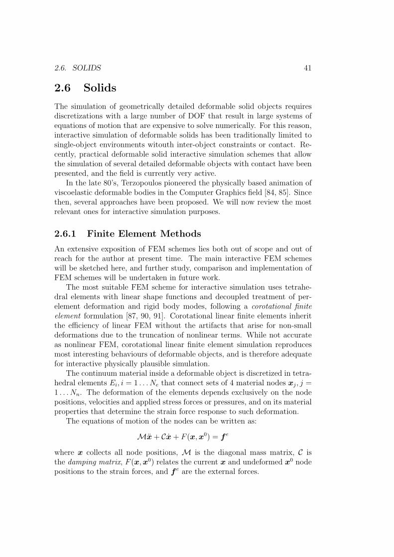
The simulation of geometrically detailed deformable solid objects requiresdiscretizations with a large number of DOF that result in large systems ofequations of motion that are expensive to solve numerically. For this reason,interactive simulation of deformable solids has been traditionally limited tosingle-object environments witouth inter-object constraints or contact. Re-cently, practical deformable solid interactive simulation schemes that allowthe simulation of several detailed deformable objects with contact have beenpresented, and the field is currently very active.
In the late 80’s, Terzopoulos pioneered the physically based animation ofviscoelastic deformable bodies in the Computer Graphics field [84, 85]. Sincethen, several approaches have been proposed. We will now review the mostrelevant ones for interactive simulation purposes.
2.6.1 Finite Element Methods
An extensive exposition of FEM schemes lies both out of scope and out ofreach for the author at present time. The main interactive FEM schemeswill be sketched here, and further study, comparison and implementation ofFEM schemes will be undertaken in future work.
The most suitable FEM scheme for interactive simulation uses tetrahe-dral elements with linear shape functions and decoupled treatment of per-element deformation and rigid body modes, following a corotational finiteelement formulation [87, 90, 91]. Corotational linear finite elements inheritthe efficiency of linear FEM without the artifacts that arise for non-smalldeformations due to the truncation of nonlinear terms. While not accurateas nonlinear FEM, corotational linear finite element simulation reproducesmost interesting behaviours of deformable objects, and is therefore adequatefor interactive physically plausible simulation.
The continuum material inside a deformable object is discretized in tetra-hedral elements Ei, i = 1 . . . Ne that connect sets of 4 material nodes xj, j =1 . . . Nn. The deformation of the elements depends exclusively on the nodepositions, velocities and applied stress forces or pressures, and on its materialproperties that determine the strain force response to such deformation.
The equations of motion of the nodes can be written as:
Mx+ Cx+ F (x,x0) = f e
where x collects all node positions, M is the diagonal mass matrix, C isthe damping matrix, F (x,x0) relates the current x and undeformed x0 nodepositions to the strain forces, and f e are the external forces.

42 CHAPTER 2. STATE OF THE ART IN INTERACTIVE DYNAMICS
For linear elasticity, F (x,x0) = K(x−x0), whereK is the stiffness matrix.The corotational formulation introduces a rigid rotation Ri for each elementthat transforms from the local coordinate frame of element i to the globalframe. Assembling all Ri into R the equations of motion become:
Mx+ Cx+RK(RTx− x0) = f e (2.15)
Given the previous and current positions of the 4 nodes forming a tetra-hedral element, the undergone rigid rotation and deformation can be approx-imated with a fast QR decomposition or exatly computed (yielding minimumdeformation) with a more involved polar decomposition [90]. The QR decom-position is reported to be robust and accurate enough for most interactivepurposes. This decomposition must be recomputed at every timestep forevery element, and therefore has a noticeable impact in the total runningtime.
Equation (2.15) can be integrated using any implicit or explicit scheme.If elastic forces are stiff, an implicit scheme such as the previously reviewedBackwards Euler method for cloth simulation 2.4 is recommended. Promisingrunning times were reported for this method in 2005 [90] (30 fps for 2000-3000 tetrahedra using BE with a time step of 0.4 ms and five CG), makingit a good candidate for interactive simulation of several deformable solids invideogames and virtual surgery.
Other FEM schemes specifically conceived for interactive simulation havebeen proposed, such as the space and time adaptative sampling method ofDebunne [86]. This method is based on prescribed local refinement of thetetrahedral mesh in order to allow for accurate haptic interaction at veryhigh refresh rates. While very efficient, the method is less general than thecorotational approach.
Strict volume-conserving FEM schemes have been recently presented inthe non-interactive domain [92], and show promising visually and physicallyaccurate results. Volume conservation is achieved through a node velocityprojection step that removes divergence, a technique inspired in fluid simu-lation [102]. We will consider its application to the interactive corotationalFEM scheme in our future work.
2.6.2 Mass and Spring Networks
Mass and spring simulation of deformable solids is an straighforward exten-sion of the techniques applied in cloth simulation. Even though the structureof a deformable solid object can be approximated using exclusively pair-wiseinter-particle springs, best results are obtained with the introduction of multi-

2.6. SOLIDS 43
particle energy constraints that resist stretch, shear and volume changes [88],in a formulation that is closely related to linear finite element methods.
2.6.3 Meshless Methods
Mesh based methods for the simulation of deformable objects are not the bestoption to model large deformations including melting, self contact and topo-logical changes such as fractures or cuts. These situations are particularlydramatic in FEM based simulations, as elements may become degeneratedue to collapse, inversion or overelongation. While expensive remeshing pro-cedures can alleviate the problem, a change of paradigm towards meshlessmethods has been proposed and successfully applied to melting, cutting andfracture simulation in virtual surgery and computer graphics [94, 96].
Meshless methods for the simulation of deformable solids in the computergraphics area where first proposed by Muller [94], though had been previouslyapplied in CG fluid simulation. Instead of discretizing the volume of thedeformable object in finite elements or particles with explicit connectivity,a non-uniform point cloud is used to sample the deformable material. Thepoints are called phyxels and represent a fragment of the material mass andvolume. While the phyxel mass remains constant, its distribution in space(and thus its volume and density) is represented using a spatial kernel withlocal support hi. On initialization, for each particle xi, the set of particles xj
that are inside its support hi is computed, and will be used to calculate itslocal deformation at runtime. The continuum mechanics elasticity equationsare then formulated in this material representation. Interactive rates havenot been reported but may be possible for moderate point counts.
Cutting and fracture can be incorporated to the meshless formulationby means of an inter-point visibility graph [96]. The graph is the Euclideanminimum spanning tree of the set of points augmented by edges between eachpoint and its k = 26 nearest neighbours. The graph is precomputed for theoriginal object and efficiently updated when connections must be removeddue to cuts or fractures. Interactive rates have been reported for moderatesized objects (21 fps for a model with 1334 triangles, 275 simulation nodeswith 52.4K visibility edges).
A simplified meshless method based on global least squares shape match-ing of deformed point clouds has been proposed for the interactive simula-tion of hundreds of deformable objects [95]. From the instantaneous points-particles positions a linear or quadratic deformation field is extracted andused to set an instantaneous reference position for each particle that robustlyattracts the particle, without overshooting, according to a stiffness coefficientα ∈ [0, 1]. While not physically-based, the method yields visually plausible

44 CHAPTER 2. STATE OF THE ART IN INTERACTIVE DYNAMICS
results and is appropiate for videogames.Finally, a versatile material model with implicit connectivity has been
recently presented in [97]. The model is somewhat similar to the point-basedmethod of Muller [94], but without any kind of connectivity or referenceshape. Each particle carries a local closest sphere packing lattice around it.The local lattice has 12 slots which are matched to current neighbours po-sitions (within a local support radius hi). The particle-slot correspondenceis then used to perform shape-matching in order to compute local defor-mation. This material representation allows a broad range of properties tobe represented, from stiff rigid bodies to fluids, and supports interesting ef-fects such as phase-transitions (melting, freezing) and fractures. Reportedcomputation times are quite high (18 seconds per step for 10000 particles).We believe that volumetric proximity computation is the main a bottleneckfor this scheme, as usually happens in lagrangian fluid simulation [104], butinteractive simulation of moderately sampled objects seems feasible.
2.7 Fluids
Fluids are, possibly, the most difficult physical objects to simulate in a com-puter, due to the constantly changing topology and the large number of DOFrequired to describe the state of a fluid volume. Interactive simulation of re-alistic 3D fluids is still unfeasible except for very low-detail discretizations.Fluid simulation in videogames and virtual reality is often limited to thesimulation of a heightfield surface that “ressembles” a fluid, using methodsoptimized for speed and visual detail, but lacking physical realism. Splashesand, in general, any kind of flow, are not considered. However, recent de-velopment of SPH-based fluid simulation methods and dedicated hardwareacceleration [112] are starting to change the situation.
Starting from the Navier-Stokes (NS) equations for incompressible andcompressible fluids, three fundamentally different discretization approacheshave been used in Computer Graphics: Eulerian mesh methods, Lagrangianmesh methods and Lagrangian meshless SPH.
2.7.1 Eulerian Methods
Eulerian grid methods discretize the spatial volume occupied by the fluid’smass in a fixed grid of regular or irregular cells. The discrete equations ofmotion are then formulated in this domain. Jos Stam’s Stable Fluids [102]was one of the most important contributions to Eulerian fluid simulation inCG, as it represented the first unconditionally stable method and allowed

2.7. FLUIDS 45
Figure 2.1: Fluid discretization approaches. (a) Eulerian grid, (b) Lagrangianmesh, (c) Lagrangian meshless SPH. (from [104])
large timesteps. The compact NS equations used by Stam are:
∂u
∂t= −(u · ∇)u−
1
ρ∇p+ ν∇2u+ f (2.16)
∇ · u = 0 (2.17)
where u is the velocity field, p is the pressure field, ∇ is the (gradient) vectorof spatial partial derivatives, ∇2 = ∇·∇ is the laplacian, ρ is the fluid densityand ν is the kinematic viscosity. The vector f gathers all external forcessuch as gravity. Equation (2.17) enforces mass preservation by requiring adivergence-free velocity field. Equation (2.16) describes how velocity changesdue to the effect of external forces and internal dynamics.
At each timestep ∆t, Stam’s algorithm updates the velocity field u(x) inseveral phases:
1. Force accumulation: Velocities are updated with the external forces f .
2. Advection: Velocities are advanced in the velocity flow during a step∆t, so that each grid point x gets the velocity that the grid point x−∆tu(x) had before advection. This unconditionally stable, as velocitiesare always bounded.
3. Diffussion: The effects of the viscosity term in Eq.(2.16) on the veloc-ity field are computed implicitly for stability. The projection requiressolving a SLE.
4. Projection: Divergence-free constraint Eq.(2.17) is enforced on the ve-locity field by projection. This amounts to solving a SLE.

46 CHAPTER 2. STATE OF THE ART IN INTERACTIVE DYNAMICS
Using iterative SLE solvers and graphics hardware acceleration (GPU), StableFluids has been applied to interactive fluid simulation on finely-discretizeddomains with visually pleasing results, and thus has become quite popularin CG and entertainment applications5. Its main advantages are (i) un-conditional stability, (ii) incompressibility and mass preservation, and (iii)efficiency (due to quite simple code that is easy to map to graphics hardwarestream processors). On the drawbacks side, (i) fluid tends to diffuse quitefast, smoothing sharp features and fine details, (ii) obstacle boundary condi-tions must be sampled on the eulerian grid, thus becoming artificially aligned(aliased), and finally, (iii) free fluid surfaces cannot be directly simulated.
Eulerian discretization with a similar solver enriched with fluid surfacetracking by means of level-sets (in a finer grid) and advected massless parti-cles has been deeply studied by Fedkiw and coworkers [100, 9, 10], yieldingthe most spectacular fluid simulations in CG so far. However, the presentedmethods are too expensive to be practically applied in interactive fluid sim-ulation.
2.7.2 Lagrangian Methods
Mesh-based methods
Lagrangian mesh-based methods have been used in fluid simulation in orderto improve mass preservation and boundary condition treatment. They arevery effective when moving boundaries must be taken into consideration.However, the topological changes inherent to fluid dynamics require complexand expensive remeshing processes on the fluid domain to avoid degeneracy,which makes this kind of methods unsuitable for interactive simulation.
Lagrangian meshes have been combined with Eulerian grids in the Ar-bitrary Lagrangian-Eulerian (ALE) approach in CG and engineering (FluidStructure interaction) [29]. ALE methods enable the treatment of movingboundaries by moving the lagrangian mesh according to the fluid dynamics(Eulerian grid advection or spring-like forces on grid nodes) to avoid the ele-ment degeneracy problems of pure Lagrangian methods. However, remeshingis unavoidable under large deformations or topological changes, and thus themethod is also quite complex and computationally expensive. To our knowl-edge the ALE has not been applied to interactive simulation.
5The popular indie game Plasma Pong combines Stam’s fluid solver with the classicPong game mechanics. The ball is guided by the velocity field and thus exhibits muchmore complex trajectories that completely change the gameplay of the original Pong.

2.7. FLUIDS 47
Meshless SPH methods
Meshless methods and, particularly, the Smoothed Particle Hydrodynamics(SPH) formulation and its variants, have been successfully applied to bothinteractive fluid simulation for videogames and high quality fluid simulationfor CG.
Following [104], we will now describe the SPH method. The fluid massis discretized in a set of n particles with positions {xi}, i = 1 . . . n. Particlesrepresent both a fraction of total massM =
∑imi and a volume Vi. Particle
masses remain constant through the simulation, and therefore total mass isautomatically preserved. Each particle defines a radially symmetric smooth-ing kernel ω around its center that will be used to approximate countinuousspatial magnitudes from the finite set of particles:
A(x) ≃∑
j
A(xj)ω(x− xj, h)Vj (2.18)
∇A(x) ≃∑
j
A(xj)∇ω(x− xj, h)Vj (2.19)
∇2A(x) ≃∑
j
A(xj)∇2ω(x− xj, h)Vj (2.20)
where A(x) is any scalar field in space, and h is the support distance ofthe smoothing kernel ω. Notice that the field gradient and laplacian canbe approximated as well, using only the field value at the particles and thekernel’s gradient and laplacian.
Different kernels may be designed for different applications. Keiser [104]and Muller [103] use 3 different kernels for density ωpoly, pressure ωspiky andviscosity ωlaplace interpolation.
Defining rij = xi−xj, particle density and volume can be approximatedas:
ρi ≃∑
j
mjωpoly(rij, h)
Vi =mi
ρi
The Navier-Stokes equations of motion (Eq.(2.17)-(2.16)) in Lagrangianform:
ρdv
dt= −∇p+ ν∇2v + f e (2.21)
∇ · v = 0 (2.22)
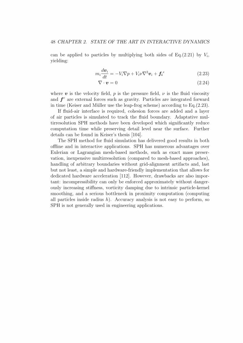
48 CHAPTER 2. STATE OF THE ART IN INTERACTIVE DYNAMICS
can be applied to particles by multiplying both sides of Eq.(2.21) by Vi,yielding:
mi
dvi
dt= −Vi∇p+ Viν∇
2vi + fie (2.23)
∇ · v = 0 (2.24)
where v is the velocity field, p is the pressure field, ν is the fluid viscosityand f e are external forces such as gravity. Particles are integrated forwardin time (Keiser and Muller use the leap-frog scheme) according to Eq.(2.23).
If fluid-air interface is required, cohesion forces are added and a layerof air particles is simulated to track the fluid boundary. Adaptative mul-tirresolution SPH methods have been developed which significantly reducecomputation time while preserving detail level near the surface. Furtherdetails can be found in Keiser’s thesis [104].
The SPH method for fluid simulation has delivered good results in bothoffline and in interactive applications. SPH has numerous advantages overEulerian or Lagrangian mesh-based methods, such as exact mass preser-vation, inexpensive multirresolution (compared to mesh-based approaches),handling of arbitrary boundaries without grid-alignment artifacts and, lastbut not least, a simple and hardware-friendly implementation that allows fordedicated hardware acceleration [112]. However, drawbacks are also impor-tant: incompressibility can only be enforced approximately without danger-ously increasing stiffness, vorticity damping due to intrinsic particle-kernelsmoothing, and a serious bottleneck in proximity computation (computingall particles inside radius h). Accuracy analysis is not easy to perform, soSPH is not generally used in engineering applications.

Chapter 3
Coupled Mechanical Systems
3.1 Problem Statement
As introduced in Section 1.2.1, realistic simulation of a mechanical systeminhabited by several mechanical objects requires accounting for inter-objectinteraction, which introduce a coupling in their equations of motion. Wewill now introduce the main concepts and notation that will be used in thegeneric treatment of coupling.
Dynamics models
In our effort towards building a generic interactive simulation frameworkwe will keep our discussion independent of any specific kind of mechanicalobject. In Chapter 2 we have reviewed different kinds of mechanical objectsas well as the specific equations of motion (dynamics models) that have beenformulated to simulate them. We will only require that the equations ofmotion conform to the second order ODE general expression:
Mq − F (q, q, t) = 0 (3.1)
which may be augmented with algebraic constraints conforming to:
g(q, q, t) = 0 (3.2)
yielding an index-3 DAE.
Mechanical coupling
Similarly, we will not focus on any specific kind of interaction. We will classifyinteractions according to the type of coupling that they generate:
49

50 CHAPTER 3. COUPLED MECHANICAL SYSTEMS
Differential coupling : Same variables appearing in equations of motion ofdifferent objects. This includes force coupling, inter-object forces de-pendent on time and objects’ configuration and motion (or related mag-nitudes)
Fij(qi, qi, qj, qj, t)
Algebraic coupling : Algebraic relationships (constraints) dependent on timeand objects’ configuration and motion (or related magnitudes)
gij(qi, qi, qj, qj) = 0
hij(qi, qi, qj, qj) > 0
Without loss of generality, we will restrict the exposition to binary forcecoupling Fij and binary constraint coupling gij = 0 or hij > 0. Objects iand j do not need to have the same kind of equations of motion (multi-modelcoupling).
Dynamics subsystems
Mechanical objects may be naturally or artificially grouped in dynamics sub-systems. Intra-subsystem inter-object coupling is assumed to be strongerand/or more frequent than inter-subsystem inter-object coupling. Similarly,a complex mechanical system may be arbitrarily decomposed in simplersubsystems for its mathematical or computational treatment. This group-ing/decomposition motivates a hierarchical view of mechanical systems.
Subsystems are assumed to evolve according to a system of equations ofmotion conforming to Eq (3.1)-(3.2), where internal constraints or interac-tions may or may not be accessible to the coupled simulation scheme. Froma mathematical point of view, no distinction between simple objects andsubsystems will be made as long as they can be described by Eq (3.1)-(3.2).
First order equations of motion
Second order equations of motion Eq (3.1) can be transformed to first order:
x− f(x, t) = 0 (3.3)
using the state vector x
x =
[q
q
]f(x, t) =
[q
M−1F (x, t)
]
Similarly, algebraic constraints Eq (3.2) can be reformulated as:
g(x, t) = 0 (3.4)
Augmenting Eq (3.3) with Eq (3.4) yields an index-2 DAE.

3.1. PROBLEM STATEMENT 51
Two-field coupling
Two-field (or two-subsystem) coupling is the simplest coupling scenario, butalready shows most important ideas and details of n-field coupling withouttoo much notational burden.
We will now formulate the coupled equations of motion of two objects orsubsystems X and Y. Differential coupling between X and Y yields a systemof first order ODE:
x− f1(x,y,u) = 0 (3.5)
y − f2(y,x,u) = 0 (3.6)
where x,y are the subsystems’ state vectors and u are global variables suchas time or control inputs.
If X and Y are algebraically coupled or subsystems have (accessible) in-ternal constraints, the global equations of motion may be augmented with:
g1(x,u) = 0 (3.7)
g2(y,u) = 0 (3.8)
g3(x,y,u) = 0 (3.9)
yielding an index-2 DAE system (3.5)-(3.9), which will be used in the follow-ing sections to illustrate different solution schemes.
Notice that f1, f2, g1, g2, g3 do not usually require all elements of subsys-tems’ states x,y. This could be explicitly modeled defining auxiliar vectorsof “shared” variables, but we prefer to keep notation as simple as possibleand thus assume that the whole state of any subsystem is accessible.
Coupling schemes
We will discuss the existing solution schemes for the DAE systems arising incoupled simulations. We are mainly interested in generic coupling schemesthat may be applied to heterogenous sets of transiently interacting objects,where the number and nature of the mechanical objects and their interactionsis not known a priori. Following [18], three main approaches exist:
Field Elimination: Some equations of motion are eliminated through sym-bolic manipulation, which often requires differentiation/integration andmay increase the order and complexity of the differential equations.
Monolithic Treatment: The whole set of coupled subsystems is treated as asingle entity and advanced simultaneously.

52 CHAPTER 3. COUPLED MECHANICAL SYSTEMS
Partitioned Treatment: Coupled subsystems are treated in isolation andindependently advanced in time. Interaction is viewed as an inter-subsystem comunication by means of prediction, substitution and syn-chronization at discrete times.
Field elimination requires complex symbolic manipulation that may notbe possible in general, and thus is discarded as a generic scheme. Monolithicand partitioned treatment are generic in nature, but have important differ-ences from numerical and software engineering perspective. We will nowintroduce the Monolithic and the Partitioned approaches in detail.
3.2 Partitioned Treatment
Partitioned treatment of coupled subsystems arises in several scenarios:
• A big mechanical entity can be decomposed in smaller subsystems ofthe same kind. Subsystems are driven by the same dinamics modelas the whole entity but have fewer DOF. Examples include domaindecomposition methods [31] and the IMEX scheme for mass and springparticle systems [78].
• A complex mechanical entity can be decomposed in heterogenous parts.This scenario arises when analyzing whole mechanisms such as vehicles,or when treating the coupling interface as an independent partition withits own dynamics [16].
• Homogenous or heterogenous preexisting entities become transientlycoupled. This is common in non-specialized virtual environments whereobjects and interactions may appear and disappear according to theapplication logic.
The third scenario is the most relevant to interactive simulation in vir-tual reality and videogames, where the structure of the virtual environmentscannot be predefined and may change during the simulation. On the otherhand, first and second scenarios are less general and more related to theoptimization and specific treatment of predefined systems.
In mechanical engineering literature, partitioning of whole systems intocoupled smaller subsystems is classified as algebraic if spatial discretizationprecedes partitioning, and differential if spatial discretization is performedafter partitioning. This distinction is mostly important in the first scenario,specifically in the decomposition of big uniform systems into smaller sub-systems of the same nature. In the second and the third scenarios onlydifferential partitioning is possible, and thus we will only discuss this case.

3.2. PARTITIONED TREATMENT 53
Partitioned treatment becomes the only option when subsystems’ equa-tions of motion or discretization details are not accessible or existing special-ized subsystem solvers must be reused.
3.2.1 Subsystem solvers
Reusing subsystems’ solvers allows us to handle each subproblem with specif-ically tailored state-of-the-art simulation schemes that are usually incompat-ible or extremely hard to integrate/extend with other schemes.
We assume that for each partition X and Y an individual solver is avail-able. These solvers may be explicit:
xn+1 = ϕ1(xn, y) (3.10)
yn+1 = ϕ2(yn, x) (3.11)
or implicit:
xn+1 = φ1(xn+1,xn, y) (3.12)
yn+1 = φ2(yn+1,yn, x) (3.13)
where x and y are given by some substitution, prediction or extrapolationoperator:
x = ψ1(xn,xn−1, . . . )
y = ψ2(yn,yn−1, . . . )
3.2.2 Devices of Partitioned Analysis
Felippa and Park [18] provide a very clear graphical language (Fig 3.1) todescribe the numerical devices of partitioned analysis and their combinationin a time-stepping program.
We will now describe these devices in some detail, assuming that thesubsystem at the top of each diagram in Fig 3.1 is X and the one at thebottom is Y:
Lockstep advancing : Both subsystems are advanced during a full step. Thisis the simplest advancing scheme.
Prediction: The next state xn+1 of subsystem X is computed using a pre-diction yn+1 of subsystem Y.
Substitution: The “exact” next state xn+1 of subsystem X is communicatedto subsystem Y and used to compute its next state yn+1 .

54 CHAPTER 3. COUPLED MECHANICAL SYSTEMS
Inter-field (fixed-point) iteration: The next states of both subsystems areiteratively corrected until they converge according to some criterion .Iteration may be expensive but increases the accuracy and stability ofthe coupling scheme.
Subcycling : Subsystem X performs several sub-steps for each full step ofsubsystem X. Systems with different time-frequencies can be coupledwithout forcing the smallest timestep on both subsystems.
Full-step correction: The next state xn+1 of subsystem X is used to correctthe current state yn of subsystem Y.
Midpoint correction: With subcycling in Y, the next state xn+1 of subsystemX is used to correct the midpoint state yn+ 1
2of subsystem Y.
Augmentation: Subsystem X is augmented/modified to incorporate somecharacteristics of subsystem Y. This has been used in Fluid-StructureInteraction to improve accuracy and stability.
Figure 3.1: Devices of partitioned analysis time stepping (from [18])
3.2.3 Partitioned schemes
Several partitioned schemes have been proposed and are regularly used inmechanical engineering [22], aeronautics [20] and fluid-structure simulation[14].
We will now overview some basic partitioned schemes. A subsystem orpartition will be qualified as explicit if its solver only uses the current state of

3.2. PARTITIONED TREATMENT 55
all subsystems, as implicit if it uses all subsystems’ future states and quasi-implicit if it uses at least one future state (usually its own) [14]. Symmetricschemes obtained by swapping {X,Y} will not be discussed.
For simplicity, we will assume that both subsystems are advanced with thesame timestep ∆t = tn+1 − tn. If one of the subsystems requires subcycling,the step index n refers to the inter-subsystem synchronization time:
(E-E) explicit-explicit coupling: This is the simplest partitioned cou-pling method, that requires no extra coupling work appart from sub-stitution:
xn+1 = ϕ1(xn, y)
yn+1 = ϕ2(yn, x)
with substitution
x = xn
y = yn
This partitioned scheme is expected to have poor stability as it’s similarto advance the whole system with an explicit integrator. Moreover, thestable coupled timestep may be smaller than the smallest of the subsys-tems’ individual stable timestep. On the other hand, the scheme is eas-ily parallelizable, which in some cases may allow for smaller timestepswhile fulfilling the efficiency requirements, and thus improve stabilityby brute force.
(I-E) implicit-explicit coupling: Prediction on Y is required to advanceX implicitly.
xn+1 = φ1(xn+1,xn, y)
yn+1 = ϕ2(yn, x)
with prediction and substitution
x = xn
y = yPn+1
This scheme treats X and Y asymmetrically, which usually comes fromcoupling different subsystem types, one being requiring implicit inte-gration for stability and the other one being well behaved enough forstable explicit integration. Parallelization is straightforward, but loadbalancing may be harder due to the asymmetric advancing schemes.

56 CHAPTER 3. COUPLED MECHANICAL SYSTEMS
(I-I) implicit-implicit coupling: Prediction on Y is required to advanceX implicitly. The newly computed state xn+1 can then be used toadvance Y implicitly.
xn+1 = φ1(xn+1,xn, y)
yn+1 = φ1(yn+1,yn, x)
with prediction and substitution
x = xn+1
y = yPn+1
This scheme is regarded as the most stable one among “simple” par-titioned methods. Parallelization is possible using prediction insteadof substitution on X, with x = xP
n+1. In this case, inter-field iterationmay be necessary to maintain accuracy-stability.
Partitioned schemes I-E and I-I are commonly referred as staggered cou-pling schemes [16]. The staggered denomination comes from the zigzaggedprediction-substitution flow in their time-stepping diagrams. Figure 3.2shows an example of I-I coupling. Removing substitution step 3 would yieldan I-E coupling scheme.
Figure 3.2: Staggered I-I sequential scheme (from [16])
Partitioned coupling schemes are usually classified as loosely coupled orstrongly coupled depending on the amount of inter-subsystem data synchro-nization performed. While strong coupling is usually required to successfullysimulate highly nonlinear coupling scenarios, several problem-specific looselycoupled schemes improved by augmentation and a careful choice of the predic-tors have been successfully applied in the Fluid-Structure Interaction (FSI)domain [20].

3.2. PARTITIONED TREATMENT 57
Loose coupling
Previously introduced E-E, I-E and I-I schemes are simple examples of loosecoupling. Loosely coupled schemes must rely on good predictors to achievereasonable accuracy and stability without requiring expensive inter-field it-eration. Algebraic coupling is not easily included and requires specific treat-ment.
When inter-subsystem algebraic coupling exists, such as in presence ofglobal constraints, loose coupling will not satisfy them. In order to accountfor algebraic coupling and avoid error accumulation, the coupling conditionsmay:
• augment one of the subsystems, thus acting as boundary conditions inits individual solver [25].
• be enforced a posteriori using some stabilization method [117], usuallyinvolving iteration or projection.
The first method treats subsystems asymmetrically and fundamentally ap-proximates a continuous two-field coupling as an interleaved sequence of one-way couplings, which may produce unrealistic effects. The second methodhas a been widely used in interactive simulation and is commonly referred aspost-stabilization.
Strong coupling
Strongly coupled schemes involve some kind of inter-field iteration in orderto accurately synchronize subsystem states, which leads to robust but com-putationally expensive algorithms. Inter-field iteration can be performed ina fixed-point fashion (as in Fig. 3.1) or in a predictor-corrector fashion [26].
Assuming an I-I scheme, we need to solve for (xn+1,yn+1) with globaliteration, so that each iteration k yields a better approximation (xk
n+1,ykn+1).
Initial estimations (x0n+1,y
0n+1) can be found using prediction.
Dropping the time-step subindex and the dependence on past “exact”states for clarity, we will now review some iteration schemes for strong cou-pling of subsystems’ solvers φ1 and φ2 that have been proposed:
Block-Jacobi: We perform global “parallel” Jacobi iterations on subsys-tems’ solvers. Global algebraic coupling is embedded in one of thesubsystems or enforced a posteriori.
xk+1 = φ1(xk,yk)
yk+1 = φ2(yk,xk)
This scheme is expected to converge very slowly.
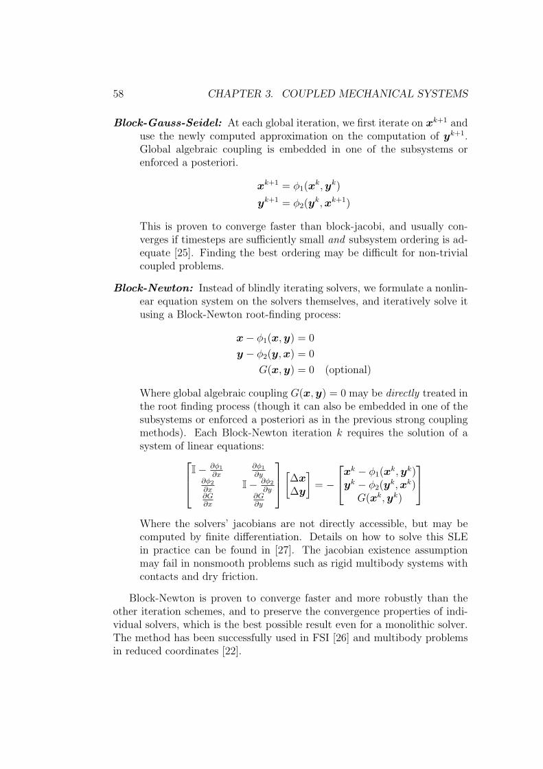
58 CHAPTER 3. COUPLED MECHANICAL SYSTEMS
Block-Gauss-Seidel: At each global iteration, we first iterate on xk+1 anduse the newly computed approximation on the computation of yk+1.Global algebraic coupling is embedded in one of the subsystems orenforced a posteriori.
xk+1 = φ1(xk,yk)
yk+1 = φ2(yk,xk+1)
This is proven to converge faster than block-jacobi, and usually con-verges if timesteps are sufficiently small and subsystem ordering is ad-equate [25]. Finding the best ordering may be difficult for non-trivialcoupled problems.
Block-Newton: Instead of blindly iterating solvers, we formulate a nonlin-ear equation system on the solvers themselves, and iteratively solve itusing a Block-Newton root-finding process:
x− φ1(x,y) = 0
y − φ2(y,x) = 0
G(x,y) = 0 (optional)
Where global algebraic coupling G(x,y) = 0 may be directly treated inthe root finding process (though it can also be embedded in one of thesubsystems or enforced a posteriori as in the previous strong couplingmethods). Each Block-Newton iteration k requires the solution of asystem of linear equations:
I− ∂φ1
∂x
∂φ1
∂y∂φ2
∂xI− ∂φ2
∂y∂G∂x
∂G∂y
[∆x
∆y
]= −
xk − φ1(x
k,yk)yk − φ2(y
k,xk)G(xk,yk)
Where the solvers’ jacobians are not directly accessible, but may becomputed by finite differentiation. Details on how to solve this SLEin practice can be found in [27]. The jacobian existence assumptionmay fail in nonsmooth problems such as rigid multibody systems withcontacts and dry friction.
Block-Newton is proven to converge faster and more robustly than theother iteration schemes, and to preserve the convergence properties of indi-vidual solvers, which is the best possible result even for a monolithic solver.The method has been successfully used in FSI [26] and multibody problemsin reduced coordinates [22].

3.2. PARTITIONED TREATMENT 59
The drawback of the Block-Newton method is its computational cost periteration, furtherly increased by the need to compute numerical derivatives.Several strategies to alleviate this fact have been proposed [23, 27].
If individual solvers are iterative, their globally iterative coupling schemecan intelligently balance the number of individual solver iterations performedfor each global iteration in order to preserve convergence while minimizingcomputation. This is commonly referred as work control, and has been stud-ied in this context by Mackens and Menck [28].
3.2.4 Fractional Steps
The coupling methods previously described assume that the subsystem up-dates are synchronized a the same discrete times. This is usually describedas a collocated scheme [20].
It has been shown that with a non-collocated scheme where subsystemsare out-of-phase by 1
2step, loosely-coupled schemes can be improved and
achieve second order accuracy without the need for inter-field iteration. Theresulting method for FSI is named Improved Serial Staggered (ISS) method(Figure 3.3).
Figure 3.3: ISS scheme (from [21])
Fractional step methods seem to be widely accepted as a computationallycheap way to improve stability and accuracy for loosely-coupled two-fieldschemes. However, their extension to n-subsystem coupling is not obvious.We plan to review fractional step methods in depth in our future work, asthey could be very useful in interactive dynamics.

60 CHAPTER 3. COUPLED MECHANICAL SYSTEMS
3.2.5 Stability and Accuracy of Partitioned Methods
In general, partitioned treatment of coupled systems is expected to be lessstable and accurate than monolithic treatment (if possible). However, themonolithic stability and accuracy orders can be usually recovered with time-step reduction, inter-field iteration or problem-specific modifications.
Stability and accuracy for staggered methods (loosely coupled) has beendeeply investigated by Felippa and Park. Most important stability results fordynamics of coupled mechanical systems are presented in [18]. It is shownthat second order oscillatory coupled systems (structure-structure) with nodamping or Rayleigh damping can be made unconditionally stable with an I-Ischeme if predictors are carefully adjusted, and that the full-system explicitintegration stability timestep limit is retained in a I-E scheme. Accuracy isanalyzed in [14] and shown to greatly depend on the integration and predictorformulas. Unfortunately, the most accurate predictors do not always ensurestability, and therefore a tradeoff emerges. These results are quite exhaustiveand the reader is referred to [18, 14] for further details.
The staggered treatment of “difficult” couplings has been shown to ben-efit from problem-specific reformulations (equation modifications [17]). Ex-amples include Fluid Structure Interaction stabilization by augmentation ofthe structure equations with fluid terms [14], and unconditionally stable andsecond order time-accurate coupled thermoelasticity simulation [19]. Recentachievements include a loosely-coupled second order time-accurate staggeredscheme for nonlinear FSI [20].
For strong coupling methods involving predictor-corrector iteration, it hasbeen shown that if a sufficient number of iterations is performed, Block-Jacobiand Block-Gauss-Seidel achieve linear convergence if subsystems’ solvers do,and Block-Newton preserves quadratic convergence if subsystems’ solvers arequadratically convergent [25]. In general, Block-Newton is considered bullet-proof and expected to converge for sufficiently small timesteps. Obviously,most stability-accuracy improvements devised for staggered schemes also ap-ply to strong coupling methods.
3.2.6 Parallelization
Parallelization of numerical methods for mechanical simulation has been ex-tensively studied and applied in order to reduce the overall computation time.There are multiple parallelization strategies (fine-grained, coarse-grained,data-parallelism, task-parallelism, etc...) and multiprocessor configurations(dual and quad core CPUs with shared memory, large CPU clusters with lo-cal memory and fast inter-processor comunication, etc...). Highest efficiency

3.2. PARTITIONED TREATMENT 61
is usually achieved with problem-specific and hardware-specific parallel algo-rithms.
In this section we are mainly interested in non-specific parallelization ofpartitioned simulation methods. The idea of partitioning a complex/largemechanical system into simpler/smaller subsystems arises naturally whencoarse-grain parallelization is taken into consideration. In addition, existingpartitioned methods are usually suitable for parallelization with small mod-ifications, as they already have some of the properties that allow efficientparallel execution:
• Data locality: Each partition/subsystem solver only requires accessto the subsystem state all the state of all its interfaces with othersubsystems, which is usually a small part of the DOF of the wholesystem.
• During a time-slice, numerical computation predominates over commu-nication and synchronization. Moreover, communication and synchro-nization patterns are predictable and remain constant, at least, duringa number of timesteps.
Several parallel partitioned schemes for two-field problems with a commoninterface appear in literature [16]. Using FSI nomenclature, the ConventionalSequential Staggered (CSS) method (Figure 3.2) can be easily parallelizedusing prediction on both fields, which results in the Conventional ParallelStaggered (CPS) method (Figure 3.4).
Figure 3.4: Staggered I-I parallel scheme (from [16])
The CPS method without inter-field iteration may seriously decrease sta-bility. However, adding inter-field itearation increases the communicationand computation cost, which may counterbalance the benefits of paralleliza-tion. For this reason, more advanced partitioned schemes have been de-veloped. Starting from the ISS method previously described, an Improved

62 CHAPTER 3. COUPLED MECHANICAL SYSTEMS
Parallel Staggered (IPS) method was developed, which achieves higher sta-bility and accuracy than the CPS. The incarnation of this method for FSIproblems is depicted in Figure 3.5.
Figure 3.5: Mid-point corrected IPS scheme with fluid subcycling (from [15])
In the related field of domain decomposition, significant speedup has beenachieved assigning each subdomain to a different CPU in a cluster configu-ration [30]. Each processor executes the same time-stepping algorithm on itsassigned subdomain and only communicating the state of its local subdomainto its neighbour subdomain processors at the end of a time-step.
3.3 Monolithic Treatment
Monolithic treatment of coupled systems is easy to describe: all equationsof motion and algebraic couplings Eqs. (3.5)-(3.9) are gathered and simul-taneously solved. This is sometimes named the direct way to solve coupledproblems, and usually amounts to solving a general index-3 or index-2 DAE.
Monolithic treatment implies a specific and global treatment of the mergedequations of motion. The numerical methods used to integrate the dynamicsforward in time and handle contacts and other constraints must be selectedwith the whole coupled system in mind. For this reason its application tomulti-model scenarios where individual models are naturally simulated us-ing different formulations or discretizations (e.g. Eulerian vs Lagrangian) isseriously restricted.
In single-model simulations, on the other hand, monolithic treatment isusually possible and may lead to highly efficient methods that exploit theuniformity of the equations of motion of all objects. State of the art methodsfor rigid multibody systems and cloth simulation are monolithic.

3.3. MONOLITHIC TREATMENT 63
3.3.1 Generic monolithic coupling
Generic differential coupling in a monolithic scheme offers no difficulty, as theinformation from all subsystems is always available to the solution process,and thus inter-subsystem forces or shared variables are trivially handled.
On the other hand, generic algebraic coupling involving different dynamicmodels and different algebraic constraints in a monolithic scheme requiressymbolically merging any combination of dynamic models and constraints.That is, all equations of motion and constraint equations must be symboli-cally transformed to a common formulation that the unified monolithic solverunderstands. Naive treatment of this fact results in a combinatorial explosionof interaction scenarios that grows intractable if n-way interaction handlingis desired. From a software engineering point of view this multiplicity iscatastrophic and has motivated specific research in symbolic pre-processingand online symbolic processing.
Symbolic pre-processing ofmulti-model andmulti-constraint coupled prob-lems is addressed by Witkin and Gleicher in [1] and [2]. The algebraic ex-pression of a constraint is decoupled from the object’s equations of motionby means of connectors, which encapsulate standard features that may beobserved on any object independently of its dynamic model (e.g. a point onits surface). This is done using the inherent black-box nature of the chainrule of differentiation.
For an algebraic constraint coupling:
C(a(qi, t), b(qj, t), t) = 0
where a and b are connector functions that extract the required informationfrom the subsystems’ configurations qi and qj. We compute the first andsecond derivatives of the constraint equations:
C(a, b, a, b, t) = 0
=d
dt(C(a, b, t))
=∂C
∂aa+
∂C
∂bb+
∂C
∂t(3.14)

64 CHAPTER 3. COUPLED MECHANICAL SYSTEMS
and
C(a, b, a, b, a, b, t) = 0
=d
dt(C(a, b, a, b, t))
=d
dt(∂C
∂aa) +
d
dt(∂C
∂bb) +
d
dt(∂C
∂t)
=∂C
∂aa+
∂C
∂bb
+ 2((∂2C
∂a∂bb)a+
∂2C
∂t∂aa+
∂2C
∂t∂bb)
+ aT∂2C
∂a2a+ bT
∂2C
∂b2b+
∂2C
∂t2(3.15)
And of the connector functions:
a =d
dt(a(qi(t), t))
=∂a
∂qi
qi +∂a
∂t(3.16)
and
a =d
dt(∂a
∂qi
qi +∂a
∂t)
=d
dt(∂a
∂qi
)qi +∂a
∂qi
qi +d
dt(∂a
∂t)
=∂a
∂qi
qi + 2∂2a
∂t∂qi
qi + qTi
∂2a
∂q2i
qi +∂2a
∂t2(3.17)
And similarly for b. The jacobians and other partial derivatives appearingin Eqs. (3.14)-(3.17) are required by general purpose DAE solvers in orderto integrate the equations of motion while fulfilling the algebraic constraints.The key contribution in [1] is that the constraints and their derivatives do notdepend directly on the objects’ configurations, but on the connectors. Thus,a single constraint definition such as the Point to Point Constraint C = P1−P2 = 0 can be combined with any pair of Point Connectors P1(qi) and P2(qj)as long as P1, P2 evaluate as points and depend only on its argument objects’configuration and time. Thus, P1 and P2 may be points on particles, on rigidobjects, on cloth surfaces, or, in general, on any dynamics model on which apoint connector can be defined. An object-oriented implementation of suchframework is straightforward, and the combinatorial explosion is reduced tosymbolically pre-processing Nconstraints +Nconnectors equations.

3.4. COUPLING INTERFACES 65
An advanced alternative to symbolic pre-processing is online symbolicprocessing. This approach, advocated by Gillespie [4] in the context of hapticinteraction, processes and assembles the equations of motion and constraintsof any specific interaction scenario at run-time. Symbolic processing mustbe performed each time that the couplings change. While this allows forcase-specific algebraic optimization that may result in efficient formulationsof the instantaneous equations of motion, online symbolic processing is tooexpensive except for very small coupled systems, specially in fast-changinginteraction scenarios such as multibody contact problems.
3.4 Coupling Interfaces
One of the most complex aspects of the simulation of coupled mechanicalsystems is the treatment of coupling interfaces. Spatial interfaces representthe domain where coupled subsystems directly interact. Spatial interactioninterfaces arise in contact problems, but also in the treatment of spatiallydiscretized models (e.g. FEM, BEM, Eulerian meshes) with partitioned anddomain decomposition methods.
Proper treatment of interfaces is of foremost importance in the couplingof nonmatching mesh discretizations, and has motivated intensive research.An exhaustive review of interface formulation methods for coupled problemsis out of scope in this introductory work. A good starting point is [32] andreferences therein.
We are mostly interested in generic contact-interface treatment betweendifferent subsystem types. This includes the coupling of nonmatching meshesand formulations of subsystems (e.g. Eulerian Fluid interacting with a La-grangian Structure, Rigid vs Cloth contact, etc). In this lines, we will focuson the work of Felippa, Park, Rebel, Ohayon and coworkers, who developedmethods based on Localized Lagrange Multipliers (LLM) that impose mini-mal restrictions on the interacting subsystems while allowing for efficient androbust partitioned treatment.
The LLM method is an extension of the Classical Lagrange Multiplier(CLM) method that is widely used in multibody contact and constrainttreatment, as well as in some deformable object contact and domain de-composition methods. The main features of the LLM are:
1. The interface is embodied, and exists somewhere inbetween coupledsubsystems. The exact interface frame placement is given by someinterpolation scheme based on coupled objects geometries [34].
2. Each subsystem is individually constrained to the interface frame in-

66 CHAPTER 3. COUPLED MECHANICAL SYSTEMS
stead of being directly constrained to other subsystems’ DOF. Thisincreases the number of required multipliers when compared to theCLM, but allows for more flexible solution techniques, and is shownto eliminate numerical difficulties derived from constraint redundancyand allow for regularization in numerically difficult scenarios [36].
This separate treatment of the interface is often classified as a three-fieldproblem, where the interface becomes an independent partition with its ownDOF and dynamics. This is very important, as it allows for more abstracthandling of contacts between heterogenous subsystems. The LLM methodhas been successfully applied to FSI and structure-structure problems, amongothers.
Figure 3.6: The LLM (a) and the CLM (b) methods for interface treatment.In LLM the interface is global (interpolated) and the multipliers (forces)are collocated at individual nodes, in CLM the multipliers are interpolated.(from [33])
Other generic interface treatment strategies are penalty methods, whichare very unstable (especially in the interactive domain), and the master-slavemethods, which impose kinematic interface boundary conditions on one orboth coupled subsystems (displacements, velocities or both), which may leadto unrealistic behaviour, as the coupling does not obey dynamics principlessuch as energy and momentum conservation). In general, these methods aredeemed inferior to the LLM and CLM [37].

3.5. COUPLED MECHANICS IN CG AND ID 67
3.5 Coupled mechanics in CG and ID
As hinted in Chapter 1, while the simulation of coupled heterogenous me-chanical systems has been widely studied in Mechanical Engineering andrelated fields, it has been scarcely addressed in Computer Graphics (CG)and almost ignored in Interactive Dynamics (ID).
Coupling in CG has been usually approached case by case, which hasresulted in coupling methods that are strongly dependent on:
1. The chosen subsystem types and their internal formulations.
2. The chosen geometric representations.
3. The numerical methods used in subsystems and in the whole coupledsystem.
This situation is not so dramatic, as specific coupling can be approximatedby physical simulation and corrected afterwards by skillful animators, whoare offered physical and unphysical tools for editing and faking realism. Evensomething as extended and “simple” as cloth animation usually requires somepost-simulation tweaking to achieve the desired realism in feature films. Two-way fluid-rigid coupling is the scenario that has undergone most intensiveresearch in CG. The fact that this is also one of the most difficult couplingsto fake or manually tweak cannot be overlooked.
In Interactive Dynamics the situation is much worse. Everything mustrun at interactive speeds and the simulation scheme must achieve robust andvisually pleasing results at first try, without post-edition. Only trial and er-ror parameter tweaking for predefined scenarios is possible (as in videogamelevels where objects are defined, placed and tested before actual play). Asa result, heterogenous coupling situations are simply ignored or treated asone-way in interactive dynamics. Examples include cloth-to-rigid interaction,rigid-to-fluid interaction and, in general, any interaction between heteroge-nous dynamics models or even between homogenous but complex dynamicsmodels (cloth-cloth, rope-rope, etc)
What is critical in both CG and ID, in our opinion, is the lack of a genericcoupling formulation and computational framework that, while not expectedto be as efficient as specific methods, allows for multi-model interaction withincremental addition or substitution of dynamics models, geometry repre-sentations and numerical solvers. For ID, the framework should be efficientenough to enable interactive simulation of moderately complex virtual worldswith current (multiprocessor) consumer hardware. The situation is startingto change, and recent efforts in virtual surgery [107, 108] and CG [109] arefinally aiming to fill this gap.

68 CHAPTER 3. COUPLED MECHANICAL SYSTEMS
In the remaining of this section, we review the coupled mechanics devel-opments in Computer Graphics research and connect them to the theoreticalbackground given in previous sections.
3.5.1 Specific two-way coupling scenarios
A number of one-way (⇒) and two-way (⇔) couplings have been studied andwill be reviewed in increasing complexity order based on dynamics models:
(P) Particles: Being the simplest model, particle interaction with mostother models has been achieved. P⇔P interactions are the basis ofparticle systems (reviewed in Section 2.1.1). P⇔RB interaction is sub-sumed in RB⇔RB interaction and thus, achieved too. P⇔DC, P⇔DSand P⇔DV interactions are not found in publications, but are easy toachieve if the DC, DS or DV is simulated as a particle-system. P⇐Finteraction has been used to add visual detail to eulerian fluid simula-tions. P⇒F interaction is subsumed in the RB⇒F case.
(RB) Rigid Bodies: Though rigid bodies have been deeply studied, re-search has been strongly biased towards RB⇔RB interactions, whichmay be considered solved for practical purposes, even though inten-sive research is still focused on the robust treatment of coulomb fric-tion (Section 2.3). RB⇔DC two-way interaction was addressed in [7].RB⇔DS interaction has been usually dealt as one-way RB⇒DS, asclothes supporting rigids may face significant mass disparity that in-troduces unstability. RB⇐DS was addressed in [82]. RB⇔DV cou-pling has been scarcely addressed, and generally handled as RB⇒DVwith projection or RB⇔DV by penalty methods. No RB⇔DV simula-tion examples of deformable objects supporting heavy rigid objects areknown to the author. RB⇔F simulation has been addressed by severalresearchers. One-way RB⇒F was investigated in [98, 99, 100]. Fastapproximate buoyancy methods for RB⇐F exist [12]. Full two-wayRB⇔F coupling was shown in [8].
(DC) Deformable Curves: Interaction with P and RB has already beenreviewed. DC⇔DC is achieved in [74], including self-collision. Noexamples of DC⇔DS, DC⇔DS and DC⇔F are known to the author.
(DS) Deformable Surfaces: Self-collision and DS⇔DS interaction areaddressed in a number of papers [75, 77, 80]. DS⇔DV does not appearspecifically in CG literature, to our knowledge. DS⇔F was addressedin [9].

3.5. COUPLED MECHANICS IN CG AND ID 69
(DV) Deformable Volumes: A method for interactive simulation of con-tacts DV⇔DV was shown in [93]. DV⇔F interaction was achieved in[11].
(F) Fluids: Only F⇔F remains to be commented. Interaction betweenfluids of differing densities and viscoelastic properties was achieved in[10].
In the following table we’ve informally collected the existence of methodsfor one-way coupling and their suitability for Interactive Dynamics:
⇒ P RB DC DS DV FL
P + + + + = =RB + + + + − −DC + + + ∅ ∅ ∅DS + − ∅ = ∅ −DV = − ∅ ∅ = −FL = + ∅ − − −
Table 3.1: One-way coupling scenarios for ID. (+ : Suitable, = : Expensive,− : Too expensive, ∅ : No published methods known).
Partitioned treatment in multibody simulation
Some ideas used in the simulation of rigid multibody systems can be intu-itively identified with similar techniques used in partitioned simulation.
1. Weinstein’s [66] black-box constraint method enforcement using themid-point of the constraint error in the next frame to correct eachobject individually can be related to the (partitioned) method of LLM.
2. Kauffman’s [64] QP-based method can be considered a partitionedscheme where each rigid body is an individual partition and uses itscontacting neighbours as boundary conditions.
3. So-called pre-stabilization methods of Bender and Weinstein, that aimto correct the predicted constraint violations in the next frame, canbe easily seen as rigid body pairwise predictor-corrector iterations in apartitioned scheme.

70 CHAPTER 3. COUPLED MECHANICAL SYSTEMS
3.5.2 Generic coupling methods
To our knowledge, the only serious research attempt to propose a generic cou-pling method in the CG field is Baraff and Witkin’s “Partitioned Dynamics”technical report [13]. This report describes a partitioned scheme for the inter-action of heterogenous subsystems through geometric constraints that onlyrequires that subsystem solvers to support holonomic constraints themselves.The scheme is very similar to a staggered partitioned treatment scheme withsubsystem jacobian-related magnitudes computed by finite-differentiation us-ing subsystem solver small steps (as in the strong coupling methods previ-ously described). The computational cost per step is reduced by avoiding in-place iteration and performing time-interleaved coupling iterations instead.Interactivity is not pursued and no performance or stability results werereported. Successful application examples include two interaction betweenrigids, clothes and particle systems. Curiously enough, the report [13] doesnot cite any reference or result from the extense body of partitioned couplingresearch existing at the moment of its writting.
In a completely different direction, a recent approach to coupled simula-tion has been pioneered by Jos Stam in the development of the Maya anima-tion software and without any related publication to date. It is based on thequite radical assumption that “all objects can be modeled with interactingparticles”. Thus, the selected approach to multi-model multi-system genericcoupling is that all objects are composed by the same low-level elements, andany object-object interaction is treated as an interaction between low-levelelements. The actual method, while unpublished, seems to be based in theconstrained particle systems described in Section 2.1.1. In an interview [109]Stam affirms that stability and directability are achieved, and that the keypoint is not having to merge different solvers but work with a unified solverfor all dynamics models. No comments on interactive performance are given.Impressive example simulation videos are shown in the references given.
A couple of open-source virtual surgery frameworks [107, 108] are cur-rently aiming at the very target of generic coupled mechanics at interactiverates. Their coupling schemes are based on penalty methods and (iterative)one-way kinematic boundary conditions, the latter easily identified as a par-titioned (strong) coupling scheme. Example simulations involve only a fewobjects and show interactive response, but further optimization would berequired to apply the methods therein to videogames.

3.6. DISCUSSION 71
3.6 Discussion
In this chapter we’ve reviewed the basic mathematical background and nu-merical methods involved in the simulation of coupled mechanical systems,with an emphasis on generic methods. Two main approaches were described:monolithic treatment and partitioned treatment, each one with its own ad-vantages and drawbacks.
We’ve seen that in Interactive Dynamics, multi-model interaction hasbeen widely avoided, as well as partitioned methods. ID has mostly reliedon fast and robust single-model monolithic methods, mainly particle sys-tems and rigid bodies in entertainment applications, and deformable models(solids, cables) with limited interaction in virtual surgery and prototyping.
In non-interactive simulation most dynamics models have been simu-lated, and most homogenous and heterogenous pairwise coupling scenarioshave been individually addressed, using both monolithic and partitioned ap-proaches. Despite a few generic schemes have been purposed, specific cou-pling methods still dominate research publications.
After reviewing previous work in specific and generic coupling methods,several simulation approaches will be now considered under the premise oftwo-level coupling: (i) inter-subsystem and (ii) multi-model inter-object cou-pling:
MMC: Monolithic-Monolithic Coupling.
Both objects and subsystems are monolithically coupled. All equationsof motion are symbolically combined either at runtime or as a pre-process, and the whole mechanical system is solved and advanced atonce.
Advantages:
• Symbolic manipulation of the equations of motion offers optimiza-tion opportunities [3].
• Stability and accuracy can be ensured using well-known ODE andDAE solvers.
Drawbacks:
• Automatic symbolic manipulation is difficult and expensive to doat runtime for moderate systems [4].
• Manual symbolic manipulation is slow and error prone, and mustface multi-model combinatorial explosion.

72 CHAPTER 3. COUPLED MECHANICAL SYSTEMS
• Changing interactions such as contacts and breaking constraintsmay require a reformulation of the equations of motion at runtime.
• Low modularity and extensibility.
• Some equations of motion may be impossible to combine symbol-ically (different formulations or discretizations).
PPC: Partitioned-Partitioned Coupling.
Every object and subsystem is treated as a black box, and no assump-tions are made about their equations of motion. Each object and sub-system is assumed to handle its own dynamics and is only required tooffer an external interaction interface (usually pressure, force, impulse,or displacement) that the partitioned simulation scheme will use tocomunicate coupling effects.
Advantages:
• Very weak assumptions on objects and subsystems. No symbolicknowledge is required.
• Independent Modeling, Modularity and Extensibility [14].
Drawbacks:
• Stability and accuracy may be difficult to achieve and their math-ematical analysis is restricted by the lack of symbolic knowledge.
• Weak assumptions on the objects’ and subsystems’ equations ofmotion complicate optimization. No uniformity or symbolic knowl-edge can be exploited.
PMHC: Partitioned-Monolithic Hybrid Coupling.
Objects are coupled monolithically and subsystems are coupled witha partitioned scheme, in an attempt to combine the best of both ap-proaches and simultaneously overcome their respective drawbacks.
Advantages:
• Weak assumptions on subsystems. No symbolic knowledge is re-quired.
• Customization, Independent Modeling, Modularity and Extensi-bility.
• Can reuse existing inter-object monolithic schemes that guaranteesolvability, efficiency and stability such as [115].

3.6. DISCUSSION 73
Drawbacks:
• Inter-object monolithic coupling implies all the drawbacks of amonolithic scheme, but alleviated by the option of treating objectsas subsystems and using a partitioned scheme.
• Stability and accuracy may be difficult to achieve for strong inter-subsystem interactions.
• Weak assumptions on the subsystems’ equations of motion com-plicate optimization. No uniformity or symbolic knowledge canbe exploited.
SMFA: Single-model-fits-all.
A single, usually simple, dynamic model is chosen for all objects [109,97]. Complex objects and subsystems are approximated as aggregatesof simple elements with inter-element constraints.
Advantages:
• Inter-object and inter-subsystem interaction is easily treated bysimple-element interactions. Neither symbolic knowledge nor blackbox assumption is required.
• Single simple dynamic model reduces mathematical and imple-mentation complexity.
• Uniformity facilitates optimization and stability.
Drawbacks:
• Certain dynamic models may not be naturally mapped into simpleelement aggregates.
• Approximation of complex dynamic models and subsystems mayrequire large amounts of simple elements, increasing processingcost when compared to a native simulation scheme.
In our opinion, “pure” simulation schemes PPC and MMC are too re-strictive. The SMFA approach has many unique advantages that make itvery appealing for interactive simulation. However, being forced to formu-late all dynamics models using the same basic representation may be toorestrictive for a truly generic simulation scheme.
A PMHC scheme that combines the flexibility of partitioned methodsfor high-level heterogenous subsystem coupling with the efficiency and ro-bustness of monolithic methods for low-level homogenous object coupling is

74 CHAPTER 3. COUPLED MECHANICAL SYSTEMS
also very attractive and may be combined with subsystems formulated us-ing the SMFA approach. Moreover, the scheme is suitable for coarse-grainparallelization (1 partition ⇔ 1 thread), as partitioned treatment and par-allel computing share similar objectives. Taking all this into account, webelieve that a framework for generic interactive simulation should be basedin the PMHC scheme. Partitioned subsystem treatment would help fulfill-ing the genericity requirement, while monolithic subsystem treatment usingstate of the art specific algorithms would allow achieving the strong efficiencyrequirements imposed by interactivity.

Chapter 4
A Framework for ICD
4.1 Objectives and Philosophy
Our motivation for building a software framework for Interactive CoupledDynamics (ICD) is twofold:
1. We want to research new coupling schemes and compare them withexisting ones in a common environment. Comparison of complex algo-rithms involving diverse numerical methods is often difficult due to un-available public implementations and differing programming languagesor methodologies. This is too often used in CG literature as an excuseto avoid direct comparison of new “improved” methods with previousones.
2. We actually want to use the framework in real-world applications as anexternal library. Moreover, we plan to develop it following the Open-Source model, so that others may use it and contribute to its improve-ment. Application fields of interest include videogames, virtual trainingand CG, but not engineering or, in general, any application field withhighy accuracy requirements.
We are conscious that the “usual” way to prototype simulation algorithmsand numerical methods is using general purpose computer algebra systems(CAS) such as Mathematica or Matlab, as they have built-in support foradvanced numerical functionality. However, we are ultimately interested ingeneric high level coupling schemes that depend on several modules specificto interactive mechanical simulation (e.g. collision detection, user interactionand control). While we know that such specific functionality may alreadyexist as extension packages for general purpose CAS or could be added us-
75

76 CHAPTER 4. A FRAMEWORK FOR ICD
ing their extensibility mechanisms, we prefer building our own simulationframework from scratch.
Developing the ICD framework as a standalone software library writtenin C++, an object-oriented programming language portable to almost everysingle platform, will allow us (and hopefully others) to actually use it in real-world multiplatform applications. Moreover, in a standalone implementationwe will be able to focus on the specific requirements of interactive simulation.
4.2 Requirements
Our first objective, using the framework as a prototyping platform for cou-pling algorithms with an emphasis on genericity, induces the following soft-ware requirements:
Extensibility: In order to use the framework as a prototyping and compar-ison tool, it should allow:
• Incremental support of dynamics models and interactions.
• Addition of simulation algorithms.
• Addition of numerical methods for standard subproblems.
Flexibility: The simulation process should be configurable:
• Configuration of physical parameters.
• Configuration of numerical parameters.
• Selection of computational methods used.
Our second objective, using the framework in real-world interactive sim-ulation applications, induces a few more requirements:
Flexibility: The simulation process should be adaptable to different situa-tions or use-cases. Flexibility can be achieved by allowing:
• Configuration of physical parameters.
• Configuration of numerical parameters.
• Configuration of execution parameters.
Efficiency: Interactivity requires a high efficiency. Several strategies arepossible:
• Asynchronous simulation in multicore platforms.

4.3. DESIGN AND ARCHITECTURE 77
• Transparent parallelization in multicore platforms.
• Platform-specific code optimization.
Interoperability: The framework should be easy to integrate into real-world applications:
• Minimal restricions on the application code.
• Simple API (Application Programming Interface).
Robustness: Detect and report errors to the application.
4.3 Design and Architecture
Taking into consideration all gathered requirements, we will now propose asuitable design. Our design will be based on the principles of object-orientedprogramming, as well as on personal experience as a developer and user ofsoftware libraries.
The Extensibility and Flexibility requirements will be addressed with animplementation based in abstract interfaces. Any predefined task for whichseveral possible implementations may be required will be invoked through anabstract interface. This includes dynamics models, interactions, numericalmethods and, at the highest level, simulation schemes.
Interoperability will be achieved by means of a carefully designed API thatwill offer access to all simulation functionality and configuration parameters.
A subset of the API will also offer a certain level of Programmability1 tothe applications, giving them access to the extensibility mechanisms of theframework in order to add or customize its own dynamics models, interac-tions, etc.
Finally, Robustness will be achieved through extensive error checking ofboth the application API calls and the execution of internal simulation tasks.Special attention will be paid to robustly handle application requests thatmay yield the simulation unstable, such as sudden object position changesor stiff forces.
Figure 4.1 shows a simplified diagram of the framework’s architecture.The most important features are a clear separation of API and CORE, whichcommunicate exclusively through Request-Answer queues. This will allow usto design the API and the actual simulation CORE independently and easilysupport asynchronous simulation. Further details will be given in followingsections.
1Hardware accelerated graphics APIs have similarly evolved from a fixed-functionpipeline to a programmable pipeline.

78 CHAPTER 4. A FRAMEWORK FOR ICD
Figure 4.1: Framework architecture draft. Arrows represent data or execu-tion flow. Diamonds represent containment relationships.
4.3.1 Dynamic entities
The virtual world (or Multiverse) will be sub-structured in:
Universe: Container of dynamic objects, organized in dynamic systems,that may eventually interact.
System : Set of dynamic objects that are simulated together.
Object : Logical representation of a physical entity.
Model : Mathematical representation of a physical entity. Typical examplesare Particles, Rigid Bodies, Deformable Solids, etc.
Each Universe may is considered a “sandbox”, which allows the ICDframework to handle several independent simulation environments concur-rently.
Systems are groups of closely interacting Objects and represent the min-imal time-stepping unit, so that all objects inside a system are advancedtogether.
Objects represent physical entities and have one or more associated Mod-els. This will allow us to eventually change the dynamic model used to simu-late a dynamic object, adding an extra level of flexibility to the developmentof coupling schemes. As an example, a Rigid Object can be internally sim-ulated using a Rigid Model (Section 2.2), a Particle System Model (Section2.1.1), or even a Meshless Solid Model (Section 2.6.3).
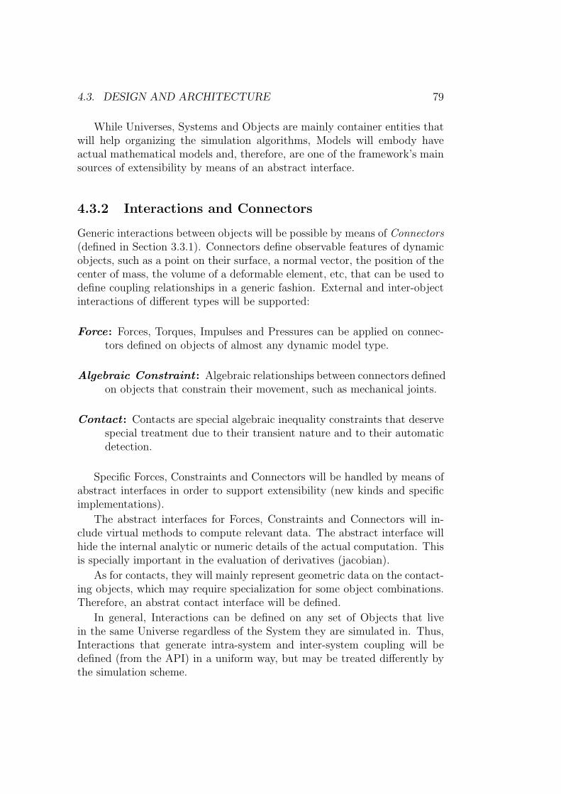
4.3. DESIGN AND ARCHITECTURE 79
While Universes, Systems and Objects are mainly container entities thatwill help organizing the simulation algorithms, Models will embody haveactual mathematical models and, therefore, are one of the framework’s mainsources of extensibility by means of an abstract interface.
4.3.2 Interactions and Connectors
Generic interactions between objects will be possible by means of Connectors(defined in Section 3.3.1). Connectors define observable features of dynamicobjects, such as a point on their surface, a normal vector, the position of thecenter of mass, the volume of a deformable element, etc, that can be used todefine coupling relationships in a generic fashion. External and inter-objectinteractions of different types will be supported:
Force: Forces, Torques, Impulses and Pressures can be applied on connec-tors defined on objects of almost any dynamic model type.
Algebraic Constraint : Algebraic relationships between connectors definedon objects that constrain their movement, such as mechanical joints.
Contact : Contacts are special algebraic inequality constraints that deservespecial treatment due to their transient nature and to their automaticdetection.
Specific Forces, Constraints and Connectors will be handled by means ofabstract interfaces in order to support extensibility (new kinds and specificimplementations).
The abstract interfaces for Forces, Constraints and Connectors will in-clude virtual methods to compute relevant data. The abstract interface willhide the internal analytic or numeric details of the actual computation. Thisis specially important in the evaluation of derivatives (jacobian).
As for contacts, they will mainly represent geometric data on the contact-ing objects, which may require specialization for some object combinations.Therefore, an abstrat contact interface will be defined.
In general, Interactions can be defined on any set of Objects that livein the same Universe regardless of the System they are simulated in. Thus,Interactions that generate intra-system and inter-system coupling will bedefined (from the API) in a uniform way, but may be treated differently bythe simulation scheme.

80 CHAPTER 4. A FRAMEWORK FOR ICD
4.3.3 Simulation Schemes
Simulation schemes are high-level algorithms that compute the evolution ofcertain dynamic entities during a time-step:
SysSS : Simulation scheme for a single System. Its responsiblilities include:
1. Detect intra-system contacts.
2. Handle intra-system Interactions (including contacts).
3. Advance all Objects inside the System.
MultiSysSS : Simulation scheme for a set of coupled Systems. It may op-tionally usie individual SysSS to perform its tasks:
1. Handle inter-system Interactions.
2. Advance all Objects inside the set of coupled Systems
UniSS : Universe simulation scheme. Its responsibilities include:
1. Detect inter-system coupling, identify independent sets of coupledSystems and create the required MultiSysSS.
2. Orchestrate the execution of SysSS and MultiSysSS in order toadvance all Objects inside the Universe.
Simulation schemes can be seen as “simulation pipelines” (homologousto graphics pipelines), as they define the high level sequence of actions toadvance the simulation during a time-step. The real benefits of this architec-ture come from the fact that simulation schemes must conform to an abstractinterface that will be used by the Kernel to execute them. This which willallow us to change the actual simulation algorithm without, hopefully, anymodification on the API or the CORE.
Simulation scheme extensibility support is expected to be extremely use-ful when prototyping coupling schemes. Specifically, MultiSysSS are respon-sible for handling inter-system coupling, so different coupling schemes couldbe prototyped and compared by switching the MultiSysSS implementationused.
4.3.4 API
The ICD framework API has been designed to be easy to use, offer exten-sive configuration functionality to facilitate its adaptation to different ap-plications, allow for efficient asynchronous execution and, last but not least,disallow or detect wrong uses that would compromise the simulation stability.

4.3. DESIGN AND ARCHITECTURE 81
The API is divided into a global API object that exposes global func-tionality and configuration, and a collection of proxy classes that representsimulation entities and simplify their creation, manipulation and querying.The set of proxy base classes can be seen in Figure 4.1. Universe and Sys-tem are thin classes to help the hierarchical construction and manipulationof simulation environments. Object, Connector and Interaction base classesmay have several derived proxy classes.
Proxy classes will offer standarized Get/Set methods to read and modifytheir state, as well as a synchronization protocol for their initialization andmodification. Proxy object lifetime starts with their creation, through theAPI. Creation does not result in any communication to the CORE. To ac-tually create a simulation entity, its proxy representation must be Defined.Definition is achieved by setting the object attributes with Set() methodsinside a BeginDefinition() / EndDefinition() block. When EndDefinition() iscalled, the proxy object is finally communicated to the CORE and insertedinto the simulation. Proxy object modification follows a similar protocol,as any modification with a Set() method will not be notified to the COREuntil its EndChanges() method is called. Get() queries to proxy objects areinexpensive, as their state is cached and retrieving it involves no communica-tion through the Request-Answer queue, while modification requests requirecommunication but can be batched inside Begin/EndChanges() blocks, thusminimizing synchronization and, most importantly, allowing the applicationto decide when it is performed.
Synchronization is automatically performed if the application requests atime-step advance on a Universe.
Programmability
We are currently investigating the best way to support a certain degree ofapplication-specific programmability to the ICD framework by taking advan-tage of the extensibility principles considered in the proposed design.
Ideally, we would allow the application to add or redefine: Models, Con-nectors, Interactions, Simulation Schemes, Numerical Methods. Two mainapproaches exist:
1. Expose the CORE abstract interfaces to the application so that it canderive new implementations and establish a mechanism that allows theapplication to send compiled classes or instances to the CORE, whowould use them through the abstract interface.
2. Design a Domain Specific Language (DLS) for writting new implemen-tations of each kind, which would be parsed by the API and sent to the

82 CHAPTER 4. A FRAMEWORK FOR ICD
CORE, who would use them through the abstract interface. This ap-proach would be similar to the mechanism currently available in graph-ics APIs for adding application-specific geometry, vertex, and fragmentprograms.
For obvious reasons, the first mechanism is easier implement, but alsomuch less secure and user-friendly. The development of a set of DSL (onefor each abstract interface) is out of our possibilities by now, but we believethat it would be the best option.
The DSLs for defining Models, Connectors and Interactions would beformula-centered, and thus could be implemented using existing symbolicmathematical parsers for C++. On the other hand, a DSL for definingSimulation Schemes would require more complex language constructs as wellas access to numerical methods and data structures existing in the CORE.An embedded scripting language (such as Lua or Python) could be used forthis purpose, but its integration raises plenty of implementation issues thatmay complicate the CORE.
4.3.5 Support functionality
Basic numerical and combinatorial algorithms are required for the implemen-tation of simulation schemes:
Linear Algebra : Vector and Matrix functionality, including dense and block-structured versions.
Quaternions: Orientation representation for Rigid Bodies and referenceframes.
ODE solvers: Basic ODE initial value problem solvers.
SLE solvers: Numerical methods to solve Systems of Linear Equations,including iterative methods (Conjugate Gradient)
SNE solvers: Numerical methods to solve Systems of Nonlinear Equations(Dense and Block Newton-Raphson)
MLCP solvers: Numerical methods to solve Mixed Linear Complemen-tarity Problems arising in Rigid Multibody dynamics.
Graphs: Data structures and basic algorithms for building and analyzingcontact and mechanical constraint graphs.
While some of this functionality has been implemented from scratch, weare currently evaluating the use of public software for the missing ones.

4.4. ENDING NOTES 83
4.4 Ending Notes
In this chapter, we’ve drafted the design of a simulation framework for Inter-active Coupled Dynamics that will allow us to prototype and compare newgeneric coupling schemes as well as to simplify the development of interactivesimulation applications.
An early prototype of such framework already exists and has been de-veloped as a personal OpenSource project called Saphyre2 and hosted atSourceForge. The interested reader may want to visit the project page athttp://saphyre.sf.net and browse and download the CVS repository, whichcontains full code as well as API, code and design documentation (with partsin Catalan).
At present, the implementation does not offer enough functionality tobe actually useful in the development of interactive applications, but thefoundations of the framework architecture as well as some simulation func-tionality are already working. Despite a lot of work remains yet to be done,we consider the current proof-of-concept implementation successful.
Currently implemented parts include:
• Framework API skeleton.
• Framework CORE abstract interfaces and Kernel.
• Request-Answer mechanism based on shared memory queues.
• A basic Universe Simulation Scheme.
• A basic System Simulation Scheme that handles Particles and Rigidswith on Point Connectors (PointOnParticle, PointOnRigid, PointStatic)and holonomic constraints (FixedDistancePoint2Point and Attached-Point2Point). The Basic SysSS is based in Baraff [53] and Witkin’s [1]force-based constrained dynamics approach with Baumgarte stabiliza-tion.
• A two-dimensional Fluid System based in the meshless SPH model.
• Two SLE solvers: LU factorization and Conjugate Gradient.
• Two ODE solvers: Forward Euler and Midpoint scheme.
• Global gravity and user defined interaction forces on Point Connectors.
All this functionality is implemented in the CORE and accessible to the API.

84 CHAPTER 4. A FRAMEWORK FOR ICD

Chapter 5
Conclusions and Future Work
In this work we were interested in reviewing the field of mechanical simulationin Interactive Dynamics and Computer Graphics applications, with specialemphasis on the treatment of coupled mechanical systems. After analyzingthe state of the art (Chapter 2), we conclude that stable and efficient meth-ods for the simulation of any kind of mechanical object are available (particlesystems, rigid bodies, rigid multibodies, ropes, wires, cables, clothes, thinshells, elastic and viscoelastic deformable solids, fluids and gaseous phenom-ena), and that almost all pairwise coupling scenarions have been addressedand practically solved (in non-interactive applications, at least). However,unrestricted n-field coupling has not been achieved as far as we know, andremains an open problem. Moreover, n-field coupling seems to be largely ig-nored by the research community, and a single research paper on the subjectis known to the author [13].
Unrestricted pairwise coupling could be theorically achieved by means of“the right combination of existing pairwise methods”. However, this strategywould be expensive and difficult to implement, and its extension to n-fieldcoupling is not clear. In our opinion, a generic approach is required tosuccessfully solve the unrestricted n-field coupling problem.
After reviewing the field of coupled mechanical simulation in MechanicalEngineering applications (Chapter 3), we’ve seen that the problem of genericcoupling has been studied in depth, and that with a partitioned approach,suitable coupling schemes can be built as long as individual solvers existand fulfill some basic requirements. The stability and accuracy propertiesof such partitioned methods have been studied and offer a solid theoreti-cal background on which robust coupling schemes can be developed. Twofamilies of partitioned methods are identified in literature: loosely-coupledschemes and strongly-coupled schemes. The former prioritize efficiency andlow inter-partition communication requirements, and rely on problem-specific
85

86 CHAPTER 5. CONCLUSIONS AND FUTURE WORK
improvements to ensure stability and accuracy, while the latter specificallyfocus on accuracy and stability, and solve a broader class of problems at theexpense of a higher computational cost.
We believe that applying existing partitioned coupling methods and sta-bility/accuracy results to interactive dynamics would enable generic and ro-bust n-field coupling, while offering new optimization opportunities. Par-ticularly, the loosely-coupled partitioned treatment of coupled mechanicalsystems shows promising parallelization advantages that could benefit fromthe multiprocessor architectures currently found in domestic computers andgaming consoles.
Moreover, the partitioned method has unique advantages from a softwareengineering perspective that would allow us to retain most of the efficiency ofexisting specific simulation methods while allowing for advanced multi-modeland inter-subsystem coupling schemes.
Taking all this into account, we think that a simulation framework basedon the partitioned approach that simplifies the prototyping and comparisonof coupling schemes would be an invaluable tool for our future work in thisfield. To our knowledge, no such framework exists that focuses on interactiveperformance while allowing for generalized interaction between heterogeneusdynamic models and systems.
A design of an interactive coupled dynamics simulation framework basedon these principles has been proposed in Chapter 4, and an early prototypehas been already implemented with satisfactory results. However, much re-mains to be done yet to achieve our objectives, and we will conclude with adescription of the future work required to advance towards our goal.
5.1 Future Work
From a theoretical perspective, we believe that the following subjects deservea much deeper analysis:
• The method of Localized Lagrange Multipliers (LLM) will be ana-lyzed and compared to the more familiar Classical Lagrange Multiplier(CLM) method. Combined with partitioned schemes, the LLM offerspromising advantages for the generic treatment of coupling interfaces.
• Loosely-coupled partitioned schemes, designed for efficiency as well asaccuracy and stability, share similar objectives with interactive simu-lation that motivate us to analyze their application to n-field genericcoupling.

5.1. FUTURE WORK 87
• The method of fractional steps offers improved stability and accuracyfor two-field coupling schemes at a very low computational cost. Itsextension to n-field generic coupling may also improve partitioned cou-pling schemes, and thus we plan to analyze it in detail.
• Parallelization of partitioned methods also requires further study. Dif-ferent parallelization strategies must be taken into account and com-pared in the specific context of interactive simulation.
On the practical side, our next steps in chronological order will be:
1. Implement a representative set of single-model simulation schemes:
(a) Fluids modeled with meshless SPH.
(b) Rigid Bodies with impulse-based collision treatment.
(c) Ropes modeled as Cosserat rods.
2. Implement several multi-system simulation schemes found in offlinesimulation literature:
(a) Loosely coupled Conventional Sequential Staggered partitionedscheme as described by Felippa et al.
(b) Strongly coupled Block-Gauss-Seidel partitioned scheme [25].
(c) Loosely coupled interleaved partitioned scheme based in [13].
3. Investigate an interface treatment method based in LLM:
(a) Interface generation.
(b) Interface constraints.
In order to develop and evaluate generic coupling schemes, a minimalset of single-model simulators must be available. We have chosen three wellstudied and substantially different models that have been successfully sim-ulated in realtime. For each model we have selected the simulation methodthat bests suits the interactive simulation requirements in terms of efficiencyand robustness.
As our main interest is to research coupling schemes, during the initialphase we will focus on 2D simulations only. This will notably shorten the im-plementation time of individual simulators, allowing us to focus on couplingschemes earlier. However, we will avoid specific 2D simplifications in thecoupling schemes that would invalidate their extension to 3D simulations.

88 CHAPTER 5. CONCLUSIONS AND FUTURE WORK
At present, the 2D Fluid simulator is almost finished, and the 2D RigidBody simulator is being developed. We have scheduled to finish the imple-mentation of the three single-system simulators in our framework by Septem-ber 2008.
Next we will implement the three coupling schemes described above andcompare them in the context of interactive simulation. In this second phasewe will focus on algebraic coupling with traditional interface modeling (CLM).We estimate that this phase will be finished in 6 months.
After evaluating these basic coupling schemes, we will investigate thebenefits of decoupling the interface DOF from the interacting models’ DOFby means of the LLM formalism, with an emphasis on the accuracy-stability-efficiency tradeoff that emerges in interactive simulation. We conservativelyestimate 6 additional months for this phase, which will end with a completecomparison of generic coupling methods. Such comparison will hopefullyguide us to a superior approach to interactive generic coupling.

Bibliography
[1] Interactive Dynamics, A.Witkin, M.Gleicher, W.Welch, CMU, 1990
[2] Spacetime Constraints, A.Witkin, M.Kass.
[3] A Survey of Multibody Dynamics for Virtual Environments, R.BrentGillespie, J.Edward Colgate, 1997.
[4] On-line Symbolic Constraint Embedding for Simulation of Hybrid Dynam-ical Systems, R. Brent Gillespie, Volkan Patoglu, Islam I. Hussein, E. R.Westervelt, Kluwer Academic Publishers, 2004.
[5] A Modeling System Based On Dynamic Constraints, Ronen Barzel, AlanH.Barr, 1988.
[6] Energy Constraints on Parametrized Models, A.Witkin, K.Fleischer,A.Barr, Proc SIGGRAPH 1987, 225-232, 1987.
[7] Mixing deformable and rigid-body mechanics simulation, J.Lenoir,S.Fonteneau, 2003.
[8] Rigid Fluid: Animating the Interplay Between Rigid Bodies and Fluid,Mark Carlson Peter J. Mucha Greg Turk, Proc. ACM SIGGRAPH 2004.
[9] Coupling water and smoke to thin deformable and rigid shells, Eran Guen-delman, Andrew Selle, Frank Losasso, Ronald Fedkiw, ACM Siggraph2005.
[10] Multiple Interacting Liquids, Losasso, F., Shinar, T. Selle, A. and Fed-kiw, R., SIGGRAPH 2006, ACM TOG 25, 812-819 (2006).
[11] Simultaneous Coupling of Fluids and Deformable Bodies, N.Chentanez,T.G.Goktekin, B.E.Feldman, J.F.O’Brien, ACM Siggrahph SCA 2006
[12] Exact Buoyancy for Polyhedra, Erin Catto, Game Programming Gems06, Charles River Media, 2006.
89

90 BIBLIOGRAPHY
[13] Partitioned Dynamics, D.Baraff, A.Witkin, Tech Report CMU-RI-TR-97-33, 1997
[14] Partitioned Analysis of Coupled Systems, C.A.Felippa, K.C.Park, Chap-ter 3 of Computational Methods for Transient Analysis, 1983.
[15] High-Performance Parallel Analysis of Coupled Problems for AircraftPropulsion, C.A. Felippa, K.C. Park, C. Farhat, CU-CAS-96-29, 1997.
[16] Partitioned Analysis of Coupled Mechanical Systems, C.A. Felippa, K.C.Park, C. Farhat, Universiy of Colorado, 1999.
[17] Equation Modification Methods, Carlos A. Felippa, 2001.
[18] Synthesis Tools for Structured Dynamics and Partitioned Analysis ofCoupled Systems, C.A.Felippa, K.C.Park, University of Colorado, 2003.
[19] An uncoditionally stable staggered algorithm for transient finite elementanalysis of coupled thermoelastic problems, C. Farhat, K. C. Park, Y.Dubois-Pelerin, Comp. Meth. Appl. Mech. Eng. 85 (1991) 349-365.
[20] SECOND-ORDER TIME-ACCURATE LOOSELY-COUPLED SOLU-TION ALGORITHMS FOR NONLINEAR FSI PROBLEMS, PhilippeGeuzaine and Kristoffer van der Zee and Charbel Farhat, ECCOMAS2004.
[21] Provably second-order time-accurate loosely-coupled solution algorithmsfor transient nonlinear computational aeroelasticity, Charbel Farhat,Kristoffer G. van der Zee, Philippe Geuzaine, Comput. Methods Appl.Mech. Engrg. 195 (2006).
[22] Simulation Algorithms in Vehicle System Dynamics, M. Arnold, Reportson Numerical Mathematics 04-27, 2004.
[23] Efficient corrector iteration for DAE time integration in multibody dy-namics, M. Arnold, A. Fuchs, C. Fuhrer, 2004.
[24] Preconditioned dynamic iteration for coupled differential-algebraic sys-tems. Arnold M, Gunther M, BIT Numerical Mathematics 2001, 41:1-25.
[25] Strong Coupling Methods, H.G.Matthies, J.Steindorf, 2002.
[26] Partitioned Strong Coupling Algorithms for Fluid-Structure-Interaction,H G. Matthies, J. Steindorf, 2002.

BIBLIOGRAPHY 91
[27] Coupling Iterative Subsystem Solvers, W. Mackens, J. Menck, H. Voss.1999.
[28] Work Control for Newton Type Coupling, J. Menck, 1999.
[29] Methods for Simulation-based Analysis of Fluid-Structure Interac-tion, Matthew F. Barone and Jeffrey L. Payne, SANDIA REPORTSAND2005-6573, 2005.
[30] PARALLEL FINITE ELEMENT METHOD FOR COUPLED CHLO-RIDE MOISTURE DIFFUSION IN CONCRETE, SUWITO, XIAO-CHUAN CAI, AND YUNPING XI, INTERNATIONAL JOURNAL OFNUMERICAL ANALYSIS AND MODELING Volume 3, Number 4,Pages 481-503, 2006.
[31] A new non conforming approach to domain decomposition: The mortarelement method, Christine Bernardi, Yvon Maday, and Anthony T. Pat-era, In Haim Brezis and Jacques-Louis Lions, editors, College de FranceSeminar. Pitman, 1994.
[32] A Survey on Contact Algorithms, N.Bourago, Proceedings of WorkshopGrid Generation: Theory and Applications, 2002.
[33] A VARIATIONAL PRINCIPLE FOR THE FORMULATION OF PAR-TITIONED STRUCTURAL SYSTEMS, K. C. Park and C. A. Felippa,CU-CAS-99-02, 1999.
[34] INTERFACING NONMATCHING FEM MESHES: THE ZERO MO-MENT RULE, K. C. Park, C. A. Felippa and G. Rebel, CU-CAS-01-01,2001.
[35] Reduced-Order Partitioned Modeling of Coupled Systems: Formulationand Computational Algorithms, K.C.Park, C.A. Felippa, R. Ohayon, Uni-versity of Colorado, 2004.
[36] Partitioned Modeling of Coupled Problems and Applications: New In-terpretations of Lagrange Multipliers, Carlos A. Felippa and K. C. Park,Presentation at WCCM-VII, Los Angeles, 17-21 July 2006.
[37] Coupling and Simulation of Acoustic Fluid-Structure Interaction Sys-tems Using Localized Lagrange Multipliers, Mike R. Ross, PhD Thesis,2004.
[38] Particle Systems – A technique for modeling a class of fuzzy objects,W.T.Reeves, ACM Transactions on Graphics 2:91-108, 1983.

92 BIBLIOGRAPHY
[39] Computational Dynamics, Ahmed A. Shabana, John Wiley & Sons, Inc.1994.
[40] Classical Mechanics, H.C. Goldstein, C.Poole, J.Safko, Addison Wesley,3rd Ed, 2002.
[41] Robot dynamics algorithms, Roy Featherstone, Kluwer 3,4 1987.
[42] Mechanical systems of rigid bodies subject to unilateral constraints, P.Lotstedt, SIAM Journal on Applied Mathematics, 42(2):281-296, 1982.
[43] An Optimized Lagrangian-Multiplier Approach for Interactive MultibodySimulations in Kinematic And Dinamical Digital Prototyping, A.Tasora.
[44] Realistic animation of rigid bodies J.K. Hahn, Proc. SIGGRAPH 88,22,4:299-308, 1988.
[45] Collision detection and response for computer animation, M. Moore andJ. Wilhelms, Proc. SIGGRAPH 88, 22,4:289-298, 1988.
[46] Impulse-based dynamic simulation of rigid bodies, MIRTICH, B., ANDCANNY, J. F. In Symposium on Interactive 3D Graphics. 1995.
[47] Timewarp rigid body simulation, B. Mirtich, In Proc. SIGGRAPH 2000,193-200.
[48] The Impulse Graph: A New Dynamic Structure for Global Collisions,George Baciu and Sai Keung Wong, Proc Eurographics Vol. 19, 2000.
[49] Analytical Methods for Dynamic Simulation of Non-penetrating RigidBodies, D. Baraff, SIGGRAPH’89, 1989.
[50] Coping with Friction for Non-penetrating Rigid Body Simulation, D.Baraff, SIGGRAPH’91, 1991.
[51] Non-penetrating Rigid Body Simulation, D. Baraff, Eurographics’93,1993.
[52] Fast Contact Force Computation for Nonpenetrating Rigid Bodies, D.Baraff, SIGGRAPH’94, 1994.
[53] Linear-Time Dynamics using Lagrange Multipliers, D. Baraff, SIG-GRAPH’96, 1996.
[54] Fast Iterative Refinement of Articulated Solid Dynamics, F.Faure, 1995.

BIBLIOGRAPHY 93
[55] Interactive Solid Animation Using Linearized Displacement Constraints,F.Faure, 1995.
[56] An Energy-Based Approach for Contact Force Computation, F. Faure.
[57] An implicit time-stepping scheme for rigid body dynamics with inelas-tic collisions and coulomb friction, D.E.Stewart, J.Trinkle, InternationalJournal for Numerical Methods in Engineering 39, 2673-2691, 1996.
[58] An Implicit Time-Stepping Scheme for Rigid body dynamics withCoulomb Friction, D.E.Stewart, J.Trinkle, 1999.
[59] Formulating dynamic multi-rigid-body contact problems with friction assolvable linear complementarity problems, M. Anitescu and F. A. Potra,Nonlinear Dynamics, 14 (1997), pp. 231-247, 1997.
[60] A time-stepping method for stiff multibody dynamics with contact andfriction, M. Anitescu and F. A. Potra, International Journal for Numer-ical Methods in Engineering 2002, 55:753-784, 2002.
[61] An iterative approach for cone complementarity problems for nonsmoothdynamics, M. Anitescu and A. Tasora, Computational Optimization andApplications (to be published), 2007.
[62] Optimization-Based Animation, Harald Schmidl, PhD Thesis, 2002.
[63] Nonconvex Rigid Bodies with Stacking, Eran Guendelman and RobertBridson and Ronald Fedkiw, ACM Transactions on Graphics (SIG-GRAPH Proc.) 22, 3 (July 2003), 871-878, 2003.
[64] Fast Frictional Dynamics for Rigid Bodies, Danny M. Kaufman andTimothy Edmunds and Dinesh K. Pai, 2004.
[65] Iterative Dynamics with Temporal Coherence, Game Developers Confer-ence (GDC), 2005.
[66] WEINSTEIN, R., TERAN, J., AND FEDKIW, R. 2005. Dynamic sim-ulation of articulated rigid bodies with contact and collision. IEEE Trans.on Vis. and Comput. Graph. (2006).
[67] Constraint-based collision and contact handling using impulses, Jan Ben-der and Alfred Schmitt, 2006.
[68] Fast Dynamic Simulation of Multi-Body Systems Using Impulses, JanBender and Alfred A. Schmitt, 2006.

94 BIBLIOGRAPHY
[69] Impulse-based dynamic simulation in linear time, Jan Bender, 2006.
[70] Splitting Methods for Dry Frictional Contact Problems in Rigid Multi-body Systems: Preliminary Performance Results, Claude Lacousiere,2006.
[71] Achim Look, Elmar Schomer, A Virtual Environment for InteractiveAssembly Simulation: From Rigid Bodies to Deformable Cables. (2001)
[72] STRANDS: Interactive Simulation of Thin Solids Using Cosserat Mod-els, Dinesh K.Pai, Eurographics 2002.
[73] Massless Cable for Real-time Simulation, M. Servin and C. Lacoursiere,unpublished, 2006.
[74] CORDE: Cosserat Rod Elements for the Dynamic Simulation of One-Dimensional Elastic Objects, J. Spillmann and M. Teschner, Eurograph-ics/ ACM SIGGRAPH Symposium on Computer Animation (2007), pp.1-10, 2007.
[75] Versatile and efficient techniques for simulating cloth and other de-formable objects, Pascal Volino and Martin Courchesne and NadiaMagnenat-Thalmann, Proc. SIGGRAPH 95, 137-144, 1995.
[76] Deformation constraints in a mass-spring model to describe rigid clothbehavior, X. Provot, In Graphics Interface, pages 147-155, 1995.
[77] Large Steps in Cloth Simulation, D.Baraff, A.Witkin, Proceedings ofSIGGRAPH 98, 43-54, 1998.
[78] Implicit-explicit schemes for fast animation with particle systems, B.Eberhardt and O. Etzmuss and M. Hauth, In Eurographics ComputerAnimation and Simulation Workshop, 2000.
[79] Advanced character physics: the fysix engine, T. Jakobsen,www.gamasutra.com, 2001.
[80] Simulation of Clothing with Folds and Wrinkles, Bridson, R., Marino, S.and Fedkiw, R., ACM SIGGRAPH/Eurographics Symposium on Com-puter Animation (SCA) pp. 28-36, 2003.
[81] Decomposing Cloth, Eddy Boxerman and Uri Ascher, Eurograph-ics/ACM SIGGRAPH Symposium on Computer Animation (2004).

BIBLIOGRAPHY 95
[82] Position Based Dynamics, M.Muller, B.Heidelberger, M.Hennix,J.Ratcliff, VRIPHYS 2006.
[83] Efficient Simulation of Inextensible Cloth, R. Goldenthal and D. Harmonand R. Fattal and M. Bercovier and E. Grispun.
[84] Elastically deformable models, TERZOPOULOS D., PLATT J., BARRA., FLEISCHER K. , In Proc SIGGRAPH 1987.
[85] Modeling Inelastic Deformation: Viscoelasticity, Plasticity, Fracture,D.Terzopoulos, K.Fleischer, In Computer Graphics (Proc. SIGGRAPH),volume 22, pages 269-278, 1988.
[86] Dynamic real-time deformations using space & time adaptive sampling,DEBUNNE, G., DESBRUN, M., CANI, M. P., AND BARR, A. H. , InComputer Graphics Proceedings, Annual Conference Series, ACM SIG-GRAPH 2001, 31-36. 2001.
[87] Stable Real-Time Deformations, Matthias Muller, Julie Dorsey, LeonardMcMillan, Robert Jagnow, Barbara Cutler, Eurographics/ACM SIG-GRAPH Symposium on Computer Animation (2002).
[88] A Versatile and Robust Model for Geometrically Complex DeformableSolids, M.Teschner, B.Heidelberger, M.Muller, M.Gross. ETH Zurich,2003.
[89] An Oriented Particle and Generalized Spring Model for Fast Prototyp-ing Deformable Objects, Il-Kwon Jeong and Inho Lee, EUROGRAPHICS2004.
[90] Effcient, physically plausible Fite elements Matthieu Nesme and YohanPayan and Francois Faure, EUROGRAPHICS 2005.
[91] Unified Formulation of Small-Strain Corotational Finite Elements: I.Theory, C. A. Felippa and B. Haugen, CU-CAS-05-02, 2005.
[92] Volume Conserving Finite Element Simulations of Deformable Objects,G. Irving, C. Schroeder, R. Fedkiw, 2007.
[93] Non-iterative Computation of Contact Forces for Deformable Objects J.Spillmann, M. Becker, M. Teschner, 2007.
[94] Point based animation of elastic, plastic and melting objects, MULLERM., KEISER R., NEALEN A., PAULY M., GROSS M., ALEXA M.,Proc. of Eurographics/ACM SIGGRAPH Symposium on Computer An-imation (2004).

96 BIBLIOGRAPHY
[95] Meshless deformations based on shape matching, MULLER M., HEI-DELBERGER B., TESCHER M., GROSS M., Proceedings of ACM Sig-graph (2005), 471-478. 2005.
[96] Fast Arbitrary Splitting of Deforming Objects, Denis Steinemann MiguelA. Otaduy Markus Gross, Eurographics/ ACM SIGGRAPH Symposiumon Computer Animation, 2006.
[97] Versatile Virtual Materials Using Implicit Connectivity, Martin Wickey,Philipp Hattz, Mark Pauly, Matthias Muller, Markus Gross. ETH Zurich- Ageia. Eurographics Symposium on Point-Based Graphics, 2006.
[98] Realistic animation of liquids, FOSTER, N., AND METAXAS, D.,Graphical Models and Image Processing 58, 5, 471-483.
[99] Controlling fluid animation, FOSTER, N., AND METAXAS, D., InProceedings CGI’97, 178-188, 1997.
[100] Practical animation of liquids, FOSTER, N., AND FEDKIW, R., InProceedings of ACM SIGGRAPH 2001, 23-30. 2001.
[101] A Vortex Particle Method for Smoke, Water and Explosions, Selle, A.,Rasmussen, N. and Fedkiw, R., SIGGRAPH 2005, ACM TOG 24, 910-914 (2005).
[102] Stable fluids, STAM, J. In Proc. of SIGGRAPH 99, 121-128. 1999.
[103] Particle-Based Fluid Simulation for Interactive Applications,M.Muller, D.Charyapar, M.Gross, ACM Siggraph SCA 2003.
[104] Meshless Lagrangian Methods for Physics-Based Animations of Solidsand Fluids, Richard Keiser, PhD Thesis, 2006.
[105] Modelica – A Language for Physical System Modeling,Visualizationand Interaction, Hilding Elmqvist, Sven Erik Mattsson, Martin Otter,CACSD’99, 1999.
[106] EVOLUTION OF CONTINUOUS-TIME MODELING AND SIMU-LATION, Karl Johan Astrom, Hilding Elmqvist, Sven Erik Mattsson,The 12th European Simulation Multiconference, ESM’98, 1998.
[107] SOFA: An Open Framework for Medical Simulation, Stephane Cotin,www.sofa-framework.org, 2007.

BIBLIOGRAPHY 97
[108] GiPSi – An Evolving Open Source / Open Architecture Software Devel-opment Framework for Surgical Simulation, http://gipsi.case.edu/, 2007.
[109] MAYA NUCLEUS, Jos Stam, http://autodesk.com/nucleus,http://features.cgsociety.org/story custom.php?story id=4026, 2007.
[110] www.naturalmotion.com
[111] www.havok.com
[112] www.ageia.com
[113] www.ode.org
[114] www.continuousphysics.com
[115] Ghosts and Machines: Regularized Variational Methods for InteractiveSimulations of Multibodies with Dry Frictional Contacts, PhD Thesis,Claude Lacousiere, 2007.
[116] Linear Complementarity, Linear and Nonlinear Programming (Inter-net Edition), Katta G. Murty, 1997.
[117] Stabilization of DAEs and invariant manifolds, Uri M. Ascher andHongsheng Chin and Sebastian Reich, Numerische Mathematik 67,2:131-149, 1994.