DEVELOPMENT OF A COUPLED THERMOHYDROLOGICAL-MECHANICAL MODEL

Prepared for

U.S. Nuclear Regulatory Commission Contract NRC–02–07–006

Prepared by

C. Manepally,1 G. Ofoegbu,1 H. Başağaoğlu,1 B. Dasgupta1

1Center for Nuclear Waste Regulatory Analyses San Antonio, Texas

and

R. Fedors2

2U.S. Nuclear Regulatory Commission

Washington, DC

December 2012

ii

ABSTRACT

This report focuses on coupled thermal-hydrological-mechanical-chemical processes, referred to as coupled processes, associated with emplacement of waste in deep underground facilities. The coupled processes can influence the barrier capabilities of the buffer and the host rock. This coupled processes report is part of the ongoing Integrated Spent Fuel Regulatory activities. This report will mainly focus on the development of a numerical modeling approach to couple thermohydrological processes with geomechanical processes. The numerical code development was to support U.S. Nuclear Regulatory Commission–Center for Nuclear Waste Regulatory Analyses (NRC–CNWRA®) participation in the DEvelopment of COupled Models and Their VALidation against EXperiments (DECOVALEX) program, whose goal is to increase understanding of coupled processes and validate models by simulating laboratory or field experiments. Much of the information in this report was presented and discussed in the joint NRC–CNWRA Coupled Processes workshop held on June 27, 2012. In the current phase of DECOVALEX (D-2015), CNWRA support to NRC will primarily be in the modeling of the HE-E test that focuses on the buffer behavior and its interaction with the host rock during the early postclosure period.

This report describes the development of a constitutive model to represent geomechanical processes in unsaturated expansive clays. The constitutive model is based on combining stresses due to suction and external loading using the principle of effective stress and deriving stress strain relationships based on elastoplasticity theory and procedures. In addition, it presents implementation of this constitutive model in FLAC. The effects of thermal load and physicochemical swelling due to moisture absorption are also accounted for in the model. Hypothetical test cases were used to verify the implementation in FLAC. Future work includes test cases using laboratory data and information from literature to verify and validate the mechanical constitutive model. A detailed description is provided in this report of the xFlo code used to represent thermohydrological processes and changes made to xFlo, including temporal variation in porosity and related parameters, in preparation for developing the linkage to FLAC and FLAC3D. Future work to couple xFlo and FLAC3D includes development of a master module that will orchestrate dynamic information exchanges and visualization of the results.

iii

CONTENTS

Section Page

ABSTRACT ................................................................................................................................... ii FIGURES ...................................................................................................................................... v TABLES ....................................................................................................................................... vii CONVERSION TABLE ............................................................................................................... viii ACKNOWLEDGMENTS .............................................................................................................. ix

1 INTRODUCTION ............................................................................................................ 1-1 1.1 Background ........................................................................................................ 1-1 1.2 DECOVALEX ..................................................................................................... 1-3 1.3 Organization of Report ....................................................................................... 1-5

2 DEVELOPMENT AND NUMERICAL IMPLEMENTATION OF A MECHANICAL CONSTITUTIVE MODEL FOR UNSATURATED EXPANSIVE CLAY SOILS ............... 2-1 2.1 Description of Constitutive Model ....................................................................... 2-2

2.1.1 The Principle of Effective Stress for Unsaturated Clay Soils .................. 2-2 2.1.2 Stress and Strain Components and Invariants ....................................... 2-3 2.1.3 Elastic Stress–Strain Relation ................................................................ 2-6 2.1.4 Plasticity Model ....................................................................................... 2-7

2.1.4.1 Yield Criterion .................................................................. 2-7 2.1.4.2 Plastic Strain Increment (Plastic Flow Rule) ................... 2-8 2.1.4.3 Evolution of Mechanical Properties During Plastic Deformation ......................................................... 2-9 2.1.4.3.1 Preconsolidation Pressure .............................................. 2-9 2.1.4.3.2 Bulk Modulus ................................................................. 2-11 2.1.4.4 Effects of Suction on Mechanical Properties ................. 2-12 2.1.4.4.1 Initial Preconsolidation Pressure ................................... 2-13 2.1.4.4.2 Reference Specific Volume ........................................... 2-13 2.1.4.4.3 Slope of the Normal-Consolidation Line ........................ 2-14 2.1.4.4.4 An Example Set of Soil Compression Parameters ........ 2-16 2.1.4.4.5 Tensile Strength ............................................................ 2-16

2.1.5 Thermal Strain ...................................................................................... 2-16 2.1.6 Physicochemically Swelling Strain ........................................................ 2-19

2.2 Implementation of Constitutive Model for Use in FLAC Computer Code ......... 2-20 2.3 Verification and Examples ................................................................................ 2-22

2.3.1 Oedometer Test of Saturated Soil ........................................................ 2-22 2.3.2 Oedometer Test of Unsaturated Soil .................................................... 2-25 2.3.3 Load-Path-Dependent Test of Unsaturated Soil ................................... 2-27 2.3.4 Swelling Example ................................................................................. 2-28

2.4 Future Work ...................................................................................................... 2-30

3 MODELING THERMOHYDROLOGICAL PROCESSES USING XFLO ......................... 3-1 3.1 Description of xFlo .............................................................................................. 3-1 3.2 Constitutive Relations for Unsaturated Flow Simulations ................................... 3-3 3.3 Calculation of Fluid Properties............................................................................ 3-4 3.4 Calculation Steps ............................................................................................... 3-7

3.4.1 Two-Phase Condition ............................................................................. 3-7 3.4.2 All-Gas Condition .................................................................................... 3-7

iv

CONTENTS (continued)

Section Page

3.4.3 No-Gas Condition ................................................................................... 3-8

3.5 Calculation of Secondary (Flux) Terms .............................................................. 3-8 3.6 Porosity-Dependent Parameters and Processes ............................................... 3-9 3.7 Future Tasks ...................................................................................................... 3-9 3.8 Potential Improvements on xFlo ......................................................................... 3-9

4 COUPLING THERMOHYDROLOGICAL AND MECHANICAL MODELS ...................... 4-1 4.1 Coupling of xFlo and FLAC3D ............................................................................ 4-1 4.2 Master Module and Post-Processor Tools ......................................................... 4-3 4.3 Example Simulations with Variable Porosity ...................................................... 4-3 4.4 Future Tasks ...................................................................................................... 4-3

5 SUMMARY ..................................................................................................................... 5-1

6 REFERENCES ............................................................................................................... 6-1

APPENDIX A—NRC-CNWRA COUPLED PROCESSES WORKSHOP AGENDA APPENDIX B—DECOVALEX D-2015 DETAILS APPENDIX C—xFlo-FLAC PARAMETERS APPENDIX D—EXAMPLE xFlo SIMULATION RESULTS

v

FIGURES

Figure Page

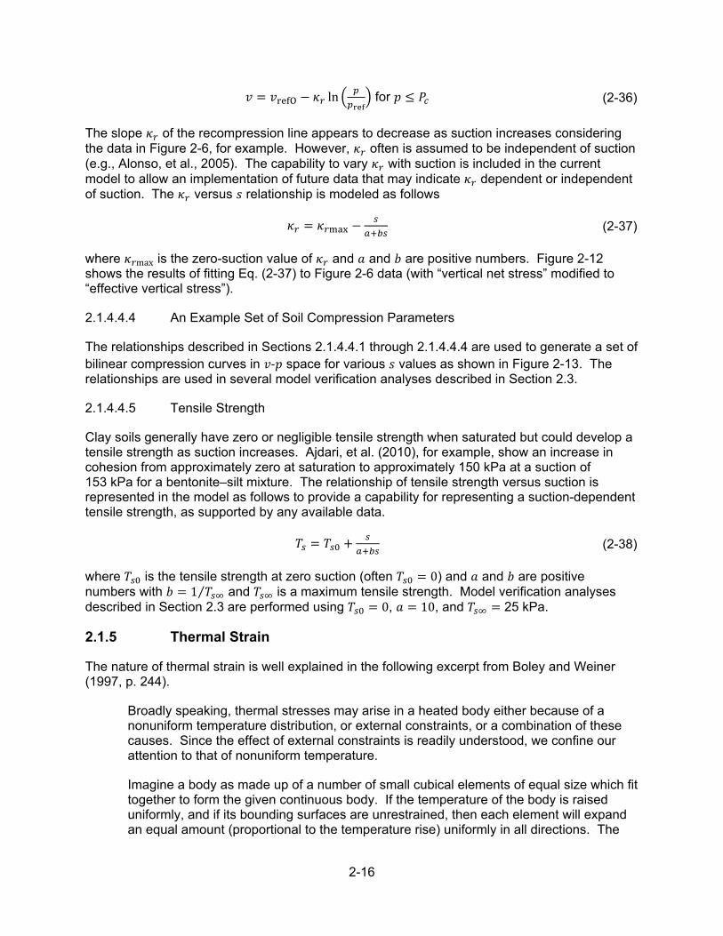
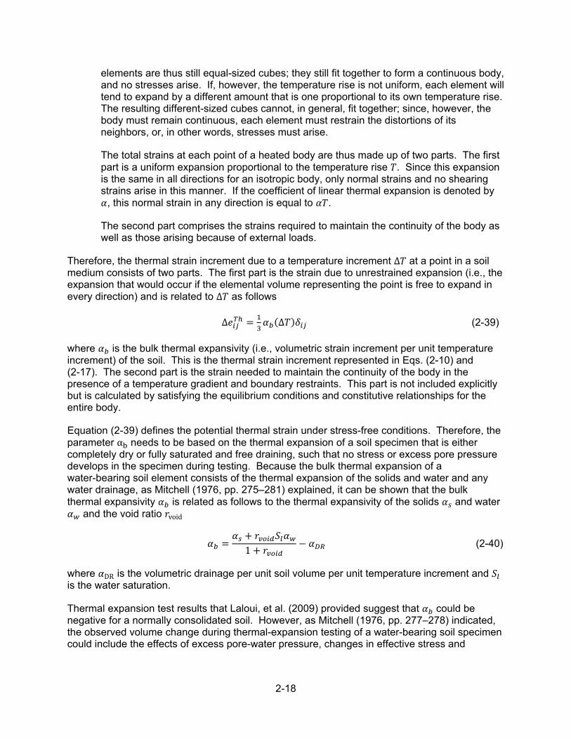
1-1 Conceptualization of Thermal-Hydrological-Mechanical-Chemical Interactions for Buffer ........................................................................................................................ 1-2 2-1 Bishop Parameter ( ) for a Sandy Silt, Based on Effective Saturation .......................... 2-4 2-2 Suction Pressure ( ) for a Sandy Silt, Based on Figure 2-1 Assuming = 0 ........................................................................................................................... 2-4 2-3 Bishop Parameter ( ) as a Function of Suction(s) for a Silt–Bentonite Mixture, Based on Curve-Fitting Data .......................................................................................... 2-5 2-4 Suction Pressure ( ) for a Silt–Bentonite Mixture, Based on Figure 2-3 ...................... 2-5 2-5 Yield Surface in − Space for Unsaturated Clay Soils ............................................... 2-8 2-6 Relationship of Void Ratio ( ) Versus Vertical Net Stress [Eq. (2-1) With = 0] for Unsaturated Bentonite–Silt Mixture at Various Values of Suction (s), Digitized .................................................................................................... 2-10 2-7 Schematic Description of a Soil Compression Curve in Terms of a Bilinear − Relationship ..................................................................................................... 2-10 2-8 Plot of a Bulk Modulus ( ) − Relationship Based on = 2.36, = 5 kPa, and ∞ = 104 kPa ..................................................................... 2-12 2-9 Plot of Initial Preconsolidation Pressure Versus Suction for a Bentonite–Silt Mixture with = 52 kPa, and M = 194 kPa From Case 3 of the Plot of Figure 2-4 ..................................................................................................... 2-14 2-10 Fitted Versus Relationship, Based on Figure 2-6 Data ..................................... 2-15 2-11 Fitted ( ) Versus Suction ( ) Relationships, Based on Eq. (2-35) and Illustrating the Effects of the Parameter with = 0.2 and = 5 × 10 5 ............. 2-15 2-12 Fitted Versus Suction ( ) Relationships Based on Eq. (2-37) and Figure 2-6 Data ............................................................................................................ 2-17 2-13 Suction(s)-Dependent Compression Curves for a Bentonite–Silt Mixture Based on Relationship Described in Sections 2.1.4.4.1 Through 2.1.4.4.4 ............................ 2-17 2-14 Cumulative Swelling Strain and Unit Swelling Potential for MX80 Bentonite ............... 2-20 2-15 Boundary Conditions for Oedometer Test Model ......................................................... 2-23 2-16 Mean Pressure Versus Y-Displacement Comparing FLAC CAM Clay and the Unsaturated Models ..................................................................................................... 2-23 2-17 Specific Volume Versus Logarithmic of Mean Pressure Comparing FLAC CAM Clay and the Unsaturated Models ....................................................................... 2-24 2-18 Bulk Modulus Versus Y-Displacement Comparing FLAC CAM Clay and the Unsaturated Models ..................................................................................................... 2-24 2-19 Mean Total Pressure Versus Y-Displacement for Different Suction Values in kPa ..... 2-26 2-20 Bulk Modulus Versus Y-Displacement for Different Suction Values in kPa ................. 2-26 2-21 Specific Volume Versus Effective Pressure Different Suction Values in kPa ............... 2-27 2-22 Load Path for Unsaturated Soil Test ............................................................................ 2-28 2-23 Specific Volume Versus Total Pressure for Load Path−1 ............................................ 2-29 2-24 Specific Volume Versus Total Pressure for Load Path−2 ............................................ 2-29 2-25 Swelling Pressure Versus Water Content for Four Different Values Swelling

Potential Parameter, CW ............................................................................................. 2-31

vi

FIGURES (continued)

Figure Page 4-1 A Schematic Demonstrating xFlo and FLAC3D Coupling .............................................. 4-2 4-2 One-Dimensional Flow Domain Geometry and the Thermal Loading Applied to the Flow Domain in the Test Simulation ..................................................................... 4-4

vii

TABLES

Table Page

2-1 Parameters and Data Used in the Analysis.................................................................. 2-21

3-1 Primary Variables for Each Fluid State .......................................................................... 3-3 3-2 Specific Conditions Implemented in xFlo Code for Phase Transitions ........................... 3-3

viii

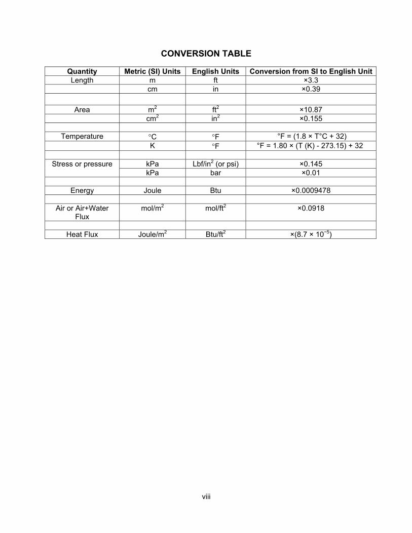
CONVERSION TABLE

Quantity Metric (SI) Units English Units Conversion from SI to English UnitLength m ft ×3.3

cm in ×0.39

Area m2 ft2 ×10.87 cm2 in2 ×0.155

Temperature C F °F = (1.8 × T°C + 32) K F °F = 1.80 × (T (K) - 273.15) + 32

Stress or pressure kPa Lbf/in2 (or psi) ×0.145 kPa bar ×0.01

Energy Joule Btu ×0.0009478

Air or Air+Water

Flux mol/m2 mol/ft2 ×0.0918

Heat Flux Joule/m2 Btu/ft2 ×(8.7 × 10−5)

ix

ACKNOWLEDGMENTS

This report was prepared to document work performed by the Center for Nuclear Waste Regulatory Analyses (CNWRA®) for the U.S. Nuclear Regulatory Commission (NRC) under Contract No. NRC–02–07–006. The activities reported here were performed on behalf of the NRC Office of Nuclear Material Safety and Safeguards, Division of Spent Fuel Alternative Strategies. The report is an independent product of CNWRA and does not necessarily reflect the views or regulatory position of NRC. The NRC staff views expressed herein are preliminary and do not constitute a final judgment or determination of the matters addressed or of the acceptability of any licensing action that may be under consideration at NRC.

The authors would like to thank M. Juckett, T. Wilt, and S. Stothoff for their technical reviews, E. Pearcy for programmatic review, and L. Mulverhill for editorial review. The authors also appreciate A. Ramos for providing word processing support in preparation of this document.

QUALITY OF DATA, ANALYSES, AND CODE DEVELOPMENT

DATA: All CNWRA-generated data contained in this report meet quality assurance requirements described in the Geosciences and Engineering Division Quality Assurance Manual. Sources of other data should be consulted for determining the level of quality of those data. The conversion factors to calculate quantities in English units are provided in the conversion table on page viii.

ANALYSES AND CODES: The computer software FLAC (Itasca Consulting Group, 2011), xFlo Version 1.0β (Painter, 2006) and MATLAB (MATLAB, 2010) were used in the analyses contained in this report. xFlo (version 1.0β) is controlled under Technical Operating Procedure (TOP)–018, Development and Control of Scientific and Engineering Software. FLAC and MATLAB are commercial software also controlled under TOP–18. Documentation for the calculations can be found in Scientific Notebooks 1103E (Ofoegbu and Dasgupta, 2011) and 1137E (Başağaoğlu, 2012).

REFERENCES

Başağaoğlu, H. “xFlo (Version 1.0β) for Thermal-Hydrological and Mechanical (THM) Simulations.” Scientific Notebook No. 1137. San Antonio, Texas: CNWRA. pp. 1–24. 2012.

Itasca Consulting Group. “FLAC V 7.0, Fast Lagrangian Analysis of Continua, User’s Guide.” Minneapolis, Minnesota: Itasca Consulting Group. 2011

MATLAB. “MATLAB User’s Guide.” Natick, Massachusetts: The MathWorks, Inc. 2010.

Ofoegbu, G.I. and B. Dasgupta. “Development of Constitutive Relations for Unsaturated Soil and Thermal-Hydrological-Mechanical Coupling.” Scientific Notebook No. 1103E. San Antonio, Texas: CNWRA. pp. 1–53. 2011.

Painter, S. “xFlo Version 1.0β User’s Manual.” San Antonio, Texas: CNWRA. 2006.

1-1

1 INTRODUCTION

This report focuses on coupled thermal-hydrological-mechanical-chemical (THMC) processes, referred to as coupled processes, associated with emplacement of waste in deep underground facilities. This coupled processes report, mainly related to thermal-hydrological-mechanical (THM) processes, is part of a number of closely related reports and workshops that comprise ongoing Integrated Spent Fuel Regulatory activities.

This is the second report related to work on coupled processes. The first report (Manepally, et al., 2011) summarized available information on coupled processes associated with deep disposal of waste in different geologic media. This report will mainly focus on the development of the numerical modeling approach to couple thermohydrological (TH) processes (using xFlo; Painter, 2006) with geomechanical processes (using FLAC, Itasca Consulting Group, 2011). The numerical code development was initiated to support U.S. Nuclear Regulatory Commission (NRC) and Center for Nuclear Waste Regulatory Analyses (CNWRA®) participation in the DEvelopment of COupled Models and Their VALidation against EXperiments (DECOVALEX) project, whose goal is to increase understanding of coupled processes and validate models by simulating large laboratory or field experiments.

Much of the information in this report was presented and discussed in a joint NRC–CNWRA Coupled Processes workshop held on June 27, 2012. The goal of the workshop was to disseminate information to and gain feedback from the NRC and CNWRA staffs on coupled processes related activities to promote integration with other Integrated Spent Fuel Regulatory activities. Workshop attendees had opportunities to discuss, add to, or expand on topics both during the topical discussions and at a roundtable discussion at the end of the workshop. Staff also identified tasks that could be considered in planning for activities to be conducted during the next fiscal year and beyond. The agenda of the Coupled Processes Workshop is provided in Appendix A.

1.1 Background

The evolution of the near-field environment influences the barrier capabilities of the waste package and engineered barrier system components such as buffer, and host rock. The changes in the hydrological, geochemical, and geomechanical properties of the buffer and host rock affect its ability to contain the waste and retard transport of radionuclides in case of waste package failure. Work in 2011 (Manepally, et al., 2011) focused on coupled processes in geologic media (argillaceous, crystalline, and salt rocks) currently being considered in international disposal programs. Buffer was also included because it is commonly a component of conceptual disposal designs, and analyses of coupled processes use similar tools to understand evolution of environmental conditions in the buffer and the rock. Based on available information, staff identified the strongly coupled processes for each geologic media and buffer material. For example, the dominant linkages for buffer include (i) the TH processes that affect the spatial and temporal distribution of saturation due to drying and rewetting of the buffer during the initial postclosure period; (ii) the degree of swelling that is controlled by the hydrological-mechanical (HM) coupling with a strong impact on the thermal pulse; (iii) the thermohydrological-chemical (THC) coupling that determines the chemical composition of the buffer that impacts the retardation capabilities of the buffer (sorption, solubility, colloid properties); and (iv) the thermal-chemical-mechanical coupling that could cause changes in mechanical properties for above-boiling conditions. Figure 1-1 illustrates prominent THMC coupled processes with a qualitative judgment of the strength of coupling. This type of figure is

1-2

Figure 1-1. Conceptualization of Thermal-Hydrological-Mechanical-Chemical Interactions for Buffer (Thick Red Solid Lines Indicate Strongly Coupled Processes, Thin Black Solid

Lines Indicate Moderately Coupled Processes, and Dashed Black Lines Indicate Uncertain or Weakly Coupled Processes)

only amenable to illustrating two-way couplings; hence, three- and four-way coupled processes are not included.

Several numerical models have been developed in the scientific community to represent coupled processes in geologic media and buffer (Manepally, et al., 2011, Table 3-1). Because fully coupled THMC model can be too computationally intensive, models that are more tractable may be created by identifying which processes should be strongly linked and which processes should be weakly linked. The latter may allow a simpler formulation to be implemented in the code, or adjustment of parameter inputs may capture the effect. Strong linkages maybe bi- or unidirectional (e.g., thermal affects mechanical, but mechanical does not significantly affect thermal conditions). Determining which processes require strong coupling or linkage in a numerical code depends on (i) the ability to accurately model conditions observed in experiments and analogs and (ii) the importance of coupled processes in the waste disposal design for performance. Information on the extent of coupling was used in the evaluation of capabilities and suitability of selected numerical models that could be used to simulate coupled processes in geologic media and buffer materials. Development of in-house capability for modeling coupled processes, rather than using existing codes from other institutions, has the

1-3

advantage of increased flexibility to add and test options for addressing new modeling components and techniques that may be useful for evaluating performance of a repository. It also helps staff to develop a deeper understanding of the applicability and limitations of models. Based on this study, it was decided that staff would develop capabilities to couple xFlo (described in Chapter 3), which represents TH processes with FLAC (described in Chapter 2) which represents geomechanical processes. The coupling of xFlo and FLAC is used to represent coupled processes in clay buffers and argillites to support participation in the DECOVALEX program. This software may also be appropriate for modeling clay buffers in granitic host rocks.

1.2 DECOVALEX

Staff conducted a survey of active international collaborative programs and concluded that participating in the DECOVALEX program would be beneficial because of the following considerations (Manepally, et al., 2011):

It provides a broad spectrum of involvement from the international community

It involves topics that focus on coupled processes

It is an opportunity for staff to leverage international experience and gain peer relations with staff from organizations from other countries

It is the most cost-efficient active collaborative group to join

Organizations participating in the DECOVALEX international consortium compare approaches and simulation results focusing on model validation using large-scale experiments and benchmark tests. The consortium’s focus is to understand coupled processes in both the emplaced buffer and the host rock of deep underground facilities for high-level waste disposal. Inherent in the DECOVALEX mission is the comparison of alternative approaches for solving complex problems that include coupled processes. Members of DECOVALEX choose to participate in one or more tasks, depending on their country’s or program’s interest. NRC staff attended previous meetings to help plan the tasks for the next phase. The next phase, D-2015, is scheduled for the period 2012 to 2015. Participants in D-2015 are listed in Table B–1 (Appendix B). D-2015 tasks are described in Table B–2.

Based on the information provided, it was decided that NRC and the CNWRA will primarily be involved in Task B1 (HE-E test). NRC staff may be involved in Task A (SEALEX) and Task C1 (THMC modeling of a single fracture). Tasks were selected based on several factors, including (i) those tasks that staff identified as technical needs and (ii) tasks involving buffer covered a wide range of applicability for processes and models and are therefore relevant to the current status of the U.S. repository program, for which the geologic media, repository conditions and design are unknown.

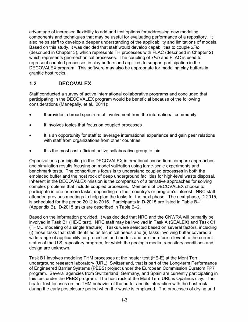
Task B1 involves modeling THM processes at the heater test (HE-E) at the Mont Terri underground research laboratory (URL), Switzerland, that is part of the Long-term Performance of Engineered Barrier Systems (PEBS) project under the European Commission Euratom FP7 program. Several agencies from Switzerland, Germany, and Spain are currently participating in this test under the PEBS program. The host rock at the Mont Terri URL is Opalinus clay. The heater test focuses on the THM behavior of the buffer and its interaction with the host rock during the early postclosure period when the waste is emplaced. The processes of drying and

1-4

subsequent resaturation of the buffer influence its swelling capacity. The HE-E test is located in the microtunnel that is approximately 10 m long and 65 cm in radius. The host rock properties (thermal, hydrological, and geomechanical) and tunnel topography have been evaluated in detail as part of the ventilation experiment (Mayor, et al., 2007) and HE-D experiment (Wileveau, 2005; Gens, et al., 2007; Wileveau and Rothfuchs, 2007; Kull, et al., 2007), which focused on the THM processes in the host rock. The buffer emplacement operations were chosen to minimize effects on the buffer properties and avoid development of fast flow paths. The influence of variation in the buffer composition on its performance is assessed by evaluating two mixtures: (i) bentonite–sand mixture and (ii) bentonite pellets. The heaters emplaced in the buffer are expected to reach a maximum temperature of 140 °C. Numerical models developed under the PEBS framework estimated a maximum temperature in the range 60–70 °C at the buffer–host rock interface. The resaturation of the buffer will follow a natural gradient determined by the host rock (i.e., no forced resaturation). The pressure, suction, displacement, temperature, and relative humidity in the buffer and surrounding host rock will be monitored. The thermal, hydrological, and mechanical properties of the bentonite pellets and bentonite blocks that support the heaters have been evaluated as a part of the PEBS project. The thermal, hydrological, and mechanical properties of the bentonite–sand mixture will be provided when data are released by the PEBS project. The modeling of the HE-E test has been divided into four steps:

1. Host Rock Characterization: Based on the HE-D experiment, evaluate THM processes in the host rock (Opalinus clay) and corresponding parameter estimates from the literature (Wileveau, 2005; Gens, et al., 2007; Wileveau and Rothfuchs, 2007). Results of this exercise will finalize the host rock’s thermal, hydrological and mechanical properties and initial conditions in the host rock to be used for the HE-E test.

2. Buffer Characterization: Evaluate (i) thermal, hydrological, and geomechanical properties and (ii) initial conditions for the sand–bentonite mixture, bentonite pellets, and bentonite blocks. The ongoing laboratory column tests results, which will be used to determine the TH input parameters of the buffer materials, will be provided later to DECOVALEX participants. Geomechanical properties of the buffer materials will be determined based on a literature review.

3. HE-E Model Development: Develop a numerical model for the HE-E test based on information available from Steps 1 and 2. The milestone product is a prediction of the THM behavior of the buffer and host rock, given the heat load. The data measured in the HE-E test will not be available for comparison at this stage.

4. HE-E Model Calibration: Based on the field observations, the HE-E model developed in Step 3 will be calibrated.

Task A (SEALEX) focuses on hydromechanical processes important for long-term performance of bentonite sealing plugs for horizontal emplacement boreholes in an argillite host rock. Laboratory and field experiments were and will be performed at approximately constant temperature conditions; thus thermal effects will not be important. The in-situ portions of the task are located at the Tournemire tunnel and experimental station in France (Barnichon, et al., 2011). The experiment is composed of 60-cm diameter, precompacted, bentonite-sand plugs that will be resaturated using water injected at both ends. The plugs are a 70/30 mixture of MX-80 bentonite and sand. Task A can be divided into four phases: (i) characterize bentonite-sand properties using laboratory data; (ii) simulate a laboratory scale mock up experiment; (iii) simulate in-situ water loss to the host rock (i.e., Toarcian Argillites); and

1-5

(iv) simulate conditions in two large-scale in-situ sealing experiments. The expectation for the first year of the DECOVALEX task is to characterize the properties required for the large-scale in-situ test using laboratory measurements of (i) the water retention curve under constant volume and under a free-swelling condition, (ii) infiltration tests under constant volume conditions, and (iii) swelling and compression tests under constant water potential (suction) conditions. Simulations of swelling and compression tests in item (iii) can rely on the geomechanical software described in Section 2 of this report. Item (i) is a simple fitting exercise and item (iii) will require the xFlo-FLAC linked software to be developed in the coming year, as described in Section 4 of this report. Also, during the first year, the characterization of the bentonite–sand properties based on the laboratory measurements (items i–iii, above) will be checked using data from a 1/10-scale laboratory mockup test. Simulations of the underground tests at Tournemire experimental station are slated for the following 2 years. Two issues that may need to be addressed in the future are hysteresis of the water retention curve and the potential formation of a bentonite gel forming near gaps and voids.

Task C1 considers THMC processes in a single fracture. The focus is on changes in hydraulic properties of a single fracture under an applied mechanical stress under different thermal conditions. The changes in hydraulic properties are caused by changes in fracture apertures due to (i) mechanical closing of the fracture and (ii) due to mineral dissolution and precipitation. This task will not use the software described in this report and therefore, will not be discussed further.

1.3 Organization of Report

Section 2 describes the development of a constitutive model to represent geomechanical processes in unsaturated expansive clays. In addition, it presents implementation of the constitutive model in FLAC and examples of calculations performed using that implementation. Section 3 details how xFlo was used to represent thermohydrological processes and how xFlo was changed (i.e., by facilitating temporal variation in porosity and related parameters) to couple with FLAC. Section 4 details the efforts to couple xFlo and FLAC (and FLAC3D) such as development of postprocessing tools and description of a proposed master module that will orchestrate dynamic information exchanges and visualization of the results. Section 5 is a summary of this report.

2-1

2 DEVELOPMENT AND NUMERICAL IMPLEMENTATION OF A MECHANICAL CONSTITUTIVE MODEL FOR UNSATURATED

EXPANSIVE CLAY SOILS

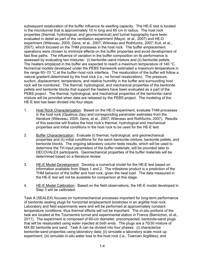
The mechanical behavior of unsaturated soils differs from saturated soils1 because of the effects of suction. Suction results from interactions between the two pore fluids (air and water) at their interfaces and increases the effective pressure that binds the soil particles. The increased effective pressure and resulting compaction of the soil skeleton can cause the soil strength and stiffness to increase. Therefore, unsaturated clay soils often exhibit greater stiffness, cohesion, and preconsolidation pressure relative to the equivalent saturated soil (cf., Alonso, et al., 1990). Expansive clay soils differ from nonexpansive clay soils because of the capability of the former (expansive clays) to undergo a chemically induced increase in volume when the soil absorbs water. All clayey soils undergo an elastic swelling when subjected to a decrease in effective pressure. However, such swelling is smaller and different from chemically induced swelling of expansive soils that could occur when the soils absorb water. In this report, the swelling is referred to as physicochemical to distinguish it from elastic swelling due to stress release. Physicochemical swelling appears to result from interactions among cations and water molecules between layers of platy clay minerals (e.g., Mitchell, 1976, p. 33).

The capability to evaluate the mechanical behavior of unsaturated expansive clay soils appears important for the assessment of the performance of nuclear waste disposal designs that include a bentonite–clay buffer or are located in an argillaceous host rock. This chapter describes the development and numerical implementation of a mechanical constitutive model for unsaturated expansive clay soils. The model is based on using the generalized principle of effective stress (Bishop, 1959 in Fredlund and Rahardjo, 1993) to combine stress contributions due to external loading with contributions due to suction. This approach differs from an existing widely used approach that is based on treating suction and stress due to external loading as two independent state variables for describing the load-deformation behavior of unsaturated soils (e.g., Alonso, et al., 1990).

In the approach based on two stress state variables, the state of stress in the soil is described in terms of the net stress NET (positive in compression) and suction defined as follows NET = − (2-1) = − (2-2)

where is the total stress (i.e., stress due to external loads); and are the air pressure and water pressure, respectively; and is the Kronecker delta ( = 1 if = and = 0 if ≠ ). The constitutive model based on this approach consists of stress-versus-strain and suction-versus-strain relationships developed using elastoplasticity based concepts with suction dependent mechanical properties (Alonso, et al., 1990).

The constitutive model described in this report is based on combining stresses due to suction and external loading using the principle of effective stress and deriving stress–strain 1Soil is used in this section as a term representing unconsolidated sediment. Expansive soil is fine-grained porous sediment that contains clay minerals that swell when wetted. The primary focus of this report is on the engineered clays referred to as bentonites or bentonite-sand mixtures, which comprise buffer or seal material in repository designs.

2-2

relationships based on elastoplasticity theory and procedures. The resulting constitutive model can be implemented in any existing geomechanics modeling code that provides an interface for implementing user-defined material models. Implementation of a material model based on two independent load-state variables (e.g., Alonso, et al., 1990) could be challenging because many solid mechanics codes (e.g., FLAC) are implemented for the state of loading in a medium to be described in terms of a single state variable, such as effective stress. For example, to implement an Alonso, et al. (1990)-type model in FLAC3D, Rutqvist, et al. (2011) introduced a suction strain increment based on an empirical suction-versus-strain relationship that was combined with other strain increments to represent the effects of suction on mechanical deformation. The approach was not adopted for the current work, because using a prescribed suction-strain relationship to account for suction contributions to elastic and inelastic deformations could be unusually problematic due to the history dependence of stress–strain relationships for inelastic deformation.

A constitutive model based on the principle of effective stress for unsaturated soils is described in Section 2.1. The implementation of the model in FLAC is described in Section 2.2, and Section 2.3 provides examples of calculations performed using the implementation.

2.1 Description of Constitutive Model

2.1.1 The Principle of Effective Stress for Unsaturated Clay Soils

The principle of effective stress for unsaturated soils (Bishop, 1959, in Fredlund and Rahardjo, 1993) describes the effective stress in terms of the total stress, suction, and air pressure (water pressure is contained in the suction term) and can be represented as follows. = + ( − ) (2-3)

Tensile stress and strain are considered positive in Eq. (2-3) and subsequent equations in this report, is the effective stress tensor (commonly denoted , but the prime symbol is not used in this report) and other symbols are as defined for Eqs. (2-1) and (2-2). In contrast to Eqs. (2-1) and (2-2) that define two independent stress state variables, Eq. (2-3) combines all stress contributions in an unsaturated soil medium into one stress state variable that can be related to strain using standard solids mechanics principles to define the constitutive behavior of unsaturated soils.

Suction and air pressure [with water pressure included through suction as defined in Eq. (2-2)] contribute a pressure term (referred to hereafter as “suction pressure” or “effective pressure due to suction”) controlled by the Bishop parameter . The pressure term can be derived from the parenthesis term in Eq. (2-3), which can be re-written as follows using Eq. (2-2). = −( − ) = −[ + (1 − ) ] (2-4)

Equation (2-4) helps understand the role of as a weighting parameter for combining fluid pressure contributions to the effective stress. The parameter varies from = 0 for a soil with air-filled voids to = 1 for a water-saturated soil [(i.e., = 1 as → 0 and = 0 as → , where is a large suction (with different values for different soils)]. Therefore, varies with water saturation in some manner and may be influenced by the continuity of the gas–water interface. A common assumption is to set equal to the water saturation (e.g., Nuth and Laloui, 2008; Dassault Systèmes, 2011). Alternatively, could be assumed equal to the effective water

2-3

saturation , which is related to the water saturation and residual water saturation as follows = ( − ) (1 − )⁄ (2-5)

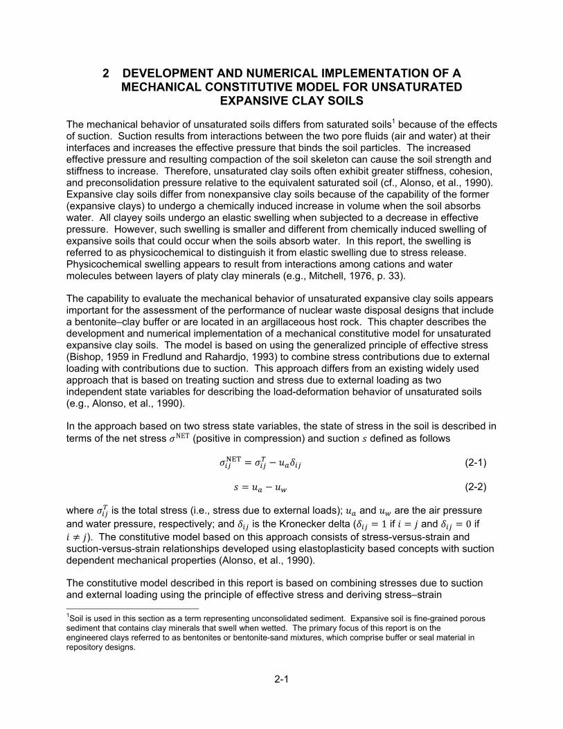
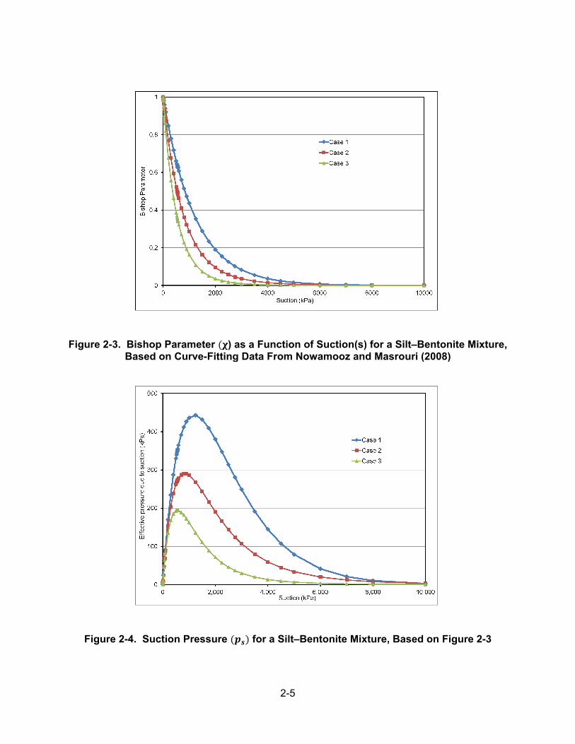
Pereira and Alonso (2009) suggested the micropore saturation could be used to represent the empirically fitted residual saturation in Eq. (2-5). They explained that pore water in clay soils consists of macropore water that is mobile and micropore water that is physicochemically (e.g., van der Waals, electrostatic forces) attached to the solid particles and, therefore, is less mobile. The capillary processes that control water flow and pressure transmission from fluids to solids in unsaturated soil are likely related more to the macropore water distribution. Figures 2-1 and 2-2 show examples of versus and versus relationships based on =

, and Figures 2-3 and 2-4 show examples of versus and versus relationships based on curve-fitting literature data without the = assumption. Using = as a basis for provides for a control of and through the soil–moisture characteristic curve (i.e., relationship between suction and moisture content or saturation).

As Figures 2-2 and 2-4 show, the relationship of versus is nonmonotonic: for small values of , increases with to a maximum value. Thereafter, decreases toward zero as increases. This nonmonotonic relationship has important implications for the effects of suction on preconsolidation pressure as discussed in Section 2.1.4.4.1.

2.1.2 Stress and Strain Components and Invariants

The constitutive model is described in terms of the effective stress tensor and total strain tensor , with and varying in the range of 1–3, and a repeated index indicates a summation over the range of the index (e.g., = + + ). For the numerical implementation of the model described in this report, the total strain tensor is calculated externally based on the equilibrium of the soil medium under the influence of any external forces and the total stress tensor T [Eq. (2-3)] and provided as an input to the constitutive model. The constitutive model describes the relationship of with the various strain contributions (e.g., due to elastic, plastic, thermal, or physicochemical swelling deformations) at a point in the soil medium.

Stress or strain increments are denoted by preceding the variable with a ∆ (e.g., ∆ represents an increment of effective stress). The stress invariants and are used in the constitutive model to represent the pressure and shearing intensity of the stress tensor, respectively, and are defined as follows = − (2-6) = 3 (2-7) = (2-8) = − (2-9)

Note that is the deviatoric stress tensor and is the second invariant of the deviatoric stress tensor. It is assumed that the possible strain contributions at a point are the elastic strain

2-4

Figure 2-1. Bishop Parameter ( ) for a Sandy Silt, Based on Effective Saturation From Fredlund and Rahardjo (1993, Figure 4.68)

Figure 2-2. Suction Pressure ( ) for a Sandy Silt, Based on Figure 2-1 Assuming = 0

2-5

Figure 2-3. Bishop Parameter ( ) as a Function of Suction(s) for a Silt–Bentonite Mixture, Based on Curve-Fitting Data From Nowamooz and Masrouri (2008)

Figure 2-4. Suction Pressure ( ) for a Silt–Bentonite Mixture, Based on Figure 2-3

2-6

, plastic strain , thermal strain Th, and physicochemical swelling strain CW. It is assumed further that the strain increments are additive and separable such that the total strain increment at a point during a change in state from time to + ∆ is related as follows to the various strain contributions ∆ = ∆ + ∆ + ∆ + ∆ (2-10)

The second assumption and, thus Eq. (2-10), is a generalization of a basic assumption used in the development of stress–strain relationships for elastic–plastic materials (e.g., Desai and Siriwardane, 1984, p. 235).

Soil strain also can be described in terms of a change in the specific volume. The specific volume at a point (i.e., representative elemental volume) in a soil medium relates the total elemental volume to the volume of solids as follows

= = 1 + (2-11)

where void represents the void ratio. (The soil porosity can be shown to be equal to ( − 1)⁄ using the relationship between porosity and void ratio.) It can be shown that the specific volume after a small volumetric strain increment is given by the equation = (1 + ∆ ) (2-12)

where O is the specific volume at the resolved state prior to the strain increment and any strain contribution due to deformation of the solid particles of the soil is assumed to be negligible (i.e., ∆ ⁄ ≈ 0).

2.1.3 Elastic Stress–Strain Relation

The effective stress increment is related to the elastic strain increment through Hooke’s law, which can be expressed as follows ∆ = ∆ (2-13)

where the elastic stiffness matrix is defined in terms of the shear modulus and Lamé parameter as follows = + + (2-14)

The parameters and are related to the bulk modulus and Poisson’s ratio as follows

= 31 + (2-15)

= 32 ( − ) (2-16)

Because the bulk modulus can vary significantly as a function of soil compaction and pressure, Eq. (2-13) is nonlinear. Therefore, is evaluated as a function of the soil deformation history as

2-7

described subsequently and and are evaluated using Eqs. (2-15) and (2-16) with an assumption of either a constant or constant .

To relate the total strain increment to the stress increment, Eq. (2-10) is substituted into Eq. (2-13) to obtain the following ∆ = ∆ − ∆ − ∆ − ∆ (2-17)

Equation (2-17) is evaluated at each material point using a total strain increment based on the equilibrium of the entire body (∆ is provided to the constitutive model as an input from an external code such as FLAC); plastic, thermal, and physicochemical swelling strain increments are based on the plasticity, thermal expansion, and physicochemical swelling models. The plasticity and physicochemical swelling models are discussed in the following sections. Thermal expansion strain is calculated using a built-in thermal expansion model in FLAC.

2.1.4 Plasticity Model

A plasticity model requires three relationships (e.g., Bathe, 1982, p. 388) viz., the yield criterion: the stress conditions that permit plastic deformation; the flow rule, which defines the plastic strain increments in relation to the stress state and stress increments; and the hardening rule, which specifies how the mechanical properties of the material evolve during plastic flow.

2.1.4.1 Yield Criterion

Following an approach Alonso, et al. (1990) used, the yield criterion is derived by modifying the CAM-Clay model yield function for saturated soils (e.g., Desai and Siriwardane, 1984, p. 282; Itasca Consulting Group, 2011, p. 1-88) to account for the effects of suction on yield strength. Based on this approach, the yield criterion is defined in terms of an elliptical surface in - space (Figure 2-5). The major axis of the ellipse lies on the axis and has a magnitude equal to + (where is the preconsolidation pressure and is the tensile strength). The minor axis of the ellipse is parallel to the axis and has a magnitude of ( 2⁄ )( + ) where is the slope of the critical state line. The equation of the yield surface (i.e., the yield function) is based on the geometry and parameters of the ellipse and is given by = + [ + ( − ) ] + ( /4)[( − ) − ( + ) ] = 0 (2-18)

The condition < 0 represents stress points within the interior of the yield surface and defines stress conditions that permit only elastic deformation. The condition = 0 represents stress points on the yield surface and defines stress conditions that permit elastic and plastic deformations. The condition > 0 is not permissible and represents a stress state that must be corrected back to the yield surface to obtain a valid elastic–plastic stress state. The yield surface may expand if increases (e.g., due to compaction) or shrink if decreases. The dependence of the yield surface on compaction (through the dependence of on compaction) implies a dependence of the yield function on the plastic volumetric strain ( P), as indicated in Figure 2-5. The location of the yield function in - space as Figure 2-5 shows is based on

being positive or zero, whereas can take negative and positive values in the range − ≤ ≤ .

2-8

Figure 2-5. Yield Surface in − Space for Unsaturated Clay Soils

2.1.4.2 Plastic Strain Increment (Plastic Flow Rule)

The flow rule defines a potential function in stress space such that the plastic strain increment is related as follows to the gradient of the function ∆ = (2-19)

where Λ is a positive scalar factor. The CAM-Clay model was developed to ensure that a plastic potential identical to the yield function (i.e., ≡ ) provides a compaction and dilation behavior consistent with the observed behavior of clay soils. Such a plastic potential is said to be “associated” with the yield function. Using such a function in Eq. (2-19) results in an associated flow rule, which implies that the plastic strain increment vector at any point on the yield surface coincides with the outward normal to the yield surface. Therefore, as indicated in Figure 2-5, plastic deformation at stress states on the right-hand side of the minor axis of the ellipse (dashed line in Figure 2-5) results in compaction. Conversely, plastic deformation at stress states on the left-hand side of the minor axis results in dilation. Plastic deformation at the stress state that represents the intersection of the minor axis with the yield surface (i.e., the so-called critical state) results in constant-volume shearing.

The following derivatives of the yield function and combinations of the derivative with the elastic stiffness matrix are needed to evaluate plastic strain increments using Eq. (2-19) = = 3 − (2 + − ) (2-20)

= = 6 − (2 + 3 )(2 + − ) (2-21)

2-9

Two alternative approaches are developed for evaluating Λ. The two approaches differ by the method used to ensure the stress state remains on the yield surface during successive stress states that permit plastic deformation.

The first approach is based on the consistency condition, which requires that ∆ = 0 for two successive stress states that permit plastic deformation (cf., Bathe, 1982, p. 388). The following relationships need to be evaluated to apply the consistency condition to the yield function defined in Eq. (2-18) ∆ = ∆ + ∆ = 0 (2-22)

The following expression is obtained for by substituting Eqs. (2-17), (2-18), (2-20), and (2-21) into Eq. (2-22) and using relationships between P and soil compaction (described subsequently in Section 2.1.4.3.1) = − − (2-23)

= + ; = − ( + ) (2-24)

where and are defined by the soil compression characteristic curve as described subsequently in Section 2.1.4.3.1. Equations (2-19) and (2-23) are used in Eq. (2-17) to calculate stress increments. The resulting stress state remains on the yield surface if the strain increment ∆ is small.

In the second approach, referred to hereafter as the quadratic equation approach, the two successive stress states are substituted into the yield function to obtain a quadratic equation in Λ. The smaller of the two roots of the equation is used as the value of Λ. The built-in CAM-Clay model of FLAC uses the quadratic equation approach.

The two approaches are implemented for the constitutive model described in this report and are shown to give identical results for a set of numerically simulated soil compression tests described subsequently in Section 2.3.

2.1.4.3 Evolution of Mechanical Properties During Plastic Deformation

2.1.4.3.1 Preconsolidation Pressure

The soil deformation state is described in terms of the specific volume . As Eq. (2-12) shows, increases as the volumetric total strain increases. An increase in indicates soil dilation,

whereas a decrease in indicates compaction. The effects of deformation on mechanical properties of clay soils are described using soil compression characteristic curves such as those shown in Figure 2-6 and described schematically in Figure 2-7. As shown in Figure 2-7, the compression curve is described in terms of a bilinear - ln relationship such as OAB. The OA segment with a slope denoted represents the unloading–reloading response and the AB segment with a slope denoted represents the virgin compression response. The unloading–reloading response is elastic whereas the virgin compression response is elastic–plastic. Therefore, the bilinear curve in the - ln space defines the boundary between elastic and elastic–plastic states along the axis.

2-10

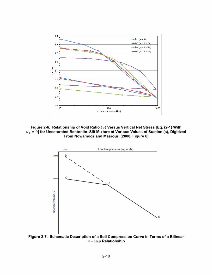
Figure 2-6. Relationship of Void Ratio ( ) Versus Vertical Net Stress [Eq. (2-1) With = ] for Unsaturated Bentonite–Silt Mixture at Various Values of Suction (s), Digitized From Nowamooz and Masrouri (2008, Figure 6)

Figure 2-7. Schematic Description of a Soil Compression Curve in Terms of a Bilinear − Relationship

2-11

The value of at point A is the preconsolidation pressure ( ), which, as described earlier in connection with Eq. (2-18), represents the maximum effective pressure that the soil experienced previously. A soil is described as “over-consolidated” if < and “normally consolidated” if = . For a normally consolidated soil, increases as the soil is compressed. However, unloading or reloading (i.e., a change in while soil is over-consolidated) does not have any effect on .

Because pressure is given on a log scale, the - ln relationship is defined relative to an arbitrary reference pressure ref (e.g., Figure 2-7). Two reference specific volumes, refN on the normal-consolidation line and refO on the over–consolidation line, can be defined at the reference pressure. At least one of the reference specific volumes needs to be defined using laboratory data. The two reference specific volumes are related as follows

N = O + ( − ) (2-25)

O = N − ( − ) ln (2-26)

The normal-consolidation line AB defines the - relationship for describing the effects of compaction on preconsolidation pressure. To formalize the - relationship, consider a deformation sequence under normal–consolidation conditions during which the specific volume and preconsolidation pressure change from ( , ) to ( + ∆ , + ∆ ). The specific volume increment consists of two parts: an elastic part Δ related to the pressure increment through

and a plastic part Δ . It can be shown using the equation of the normal–consolidation line that ∆ = −( − ) ∆

(2-27)

If the preconsolidation pressure at the resolved state (start of the deformation increment) is denoted O and the specific volume O , then it can be shown using Eqs. (2-12) and (2-27) that the preconsolidation pressure at the new state (end of the deformation increment) is given by the following

= 1 − (2-28)

2.1.4.3.2 Bulk Modulus

The soil bulk modulus also evolves during soil deformation because of the effects of compaction or dilation and pressure on soil stiffness. Using pressure versus volumetric strain relationships under over-consolidation conditions, it can be shown that the bulk modulus is given by the following = (2-29)

However, Eq. (2-29) can give unreasonably high values of as the product (denoted ) increases. Actually, should approach a limiting value (e.g., as increases). Therefore the - relationship is replaced with the following equation, which gives values of that approach a user-specified limiting value as increases (Figure 2-8)

2-12

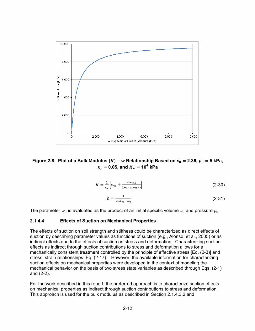
Figure 2-8. Plot of a Bulk Modulus ( ) − Relationship Based on = 2.36, = 5 kPa, = 0.05, and ∞ = 104 kPa = + ( ) (2-30)

= (2-31)

The parameter is evaluated as the product of an initial specific volume and pressure .

2.1.4.4 Effects of Suction on Mechanical Properties

The effects of suction on soil strength and stiffness could be characterized as direct effects of suction by describing parameter values as functions of suction (e.g., Alonso, et al., 2005) or as indirect effects due to the effects of suction on stress and deformation. Characterizing suction effects as indirect through suction contributions to stress and deformation allows for a mechanically consistent treatment controlled by the principle of effective stress [Eq. (2-3)] and stress–strain relationships [Eq. (2-17)]. However, the available information for characterizing suction effects on mechanical properties were developed in the context of modeling the mechanical behavior on the basis of two stress state variables as described through Eqs. (2-1) and (2-2).

For the work described in this report, the preferred approach is to characterize suction effects on mechanical properties as indirect through suction contributions to stress and deformation. This approach is used for the bulk modulus as described in Section 2.1.4.3.2 and

2-13

preconsolidation pressure as described subsequently. However, the reference specific volume refO, compressibility parameters and , and tensile strength are described as direct functions of suction because of the lack of information to relate the parameters to stress or deformation. The treatment of the suction effects on these parameters will be re-examined in the future. Also, it is assumed in this report that the strength parameter [Eq. (2-18) and Figure 2-5] is not affected by suction. This assumption is consistent with existing practice (e.g., Alonso, et al., 2005).

2.1.4.4.1 Initial Preconsolidation Pressure

The value of preconsolidation pressure at the initial state (i.e., state of zero deformation characterized by an initial pressure and initial void ratio or specific volume) init consists of two parts as follows = + (2-32)

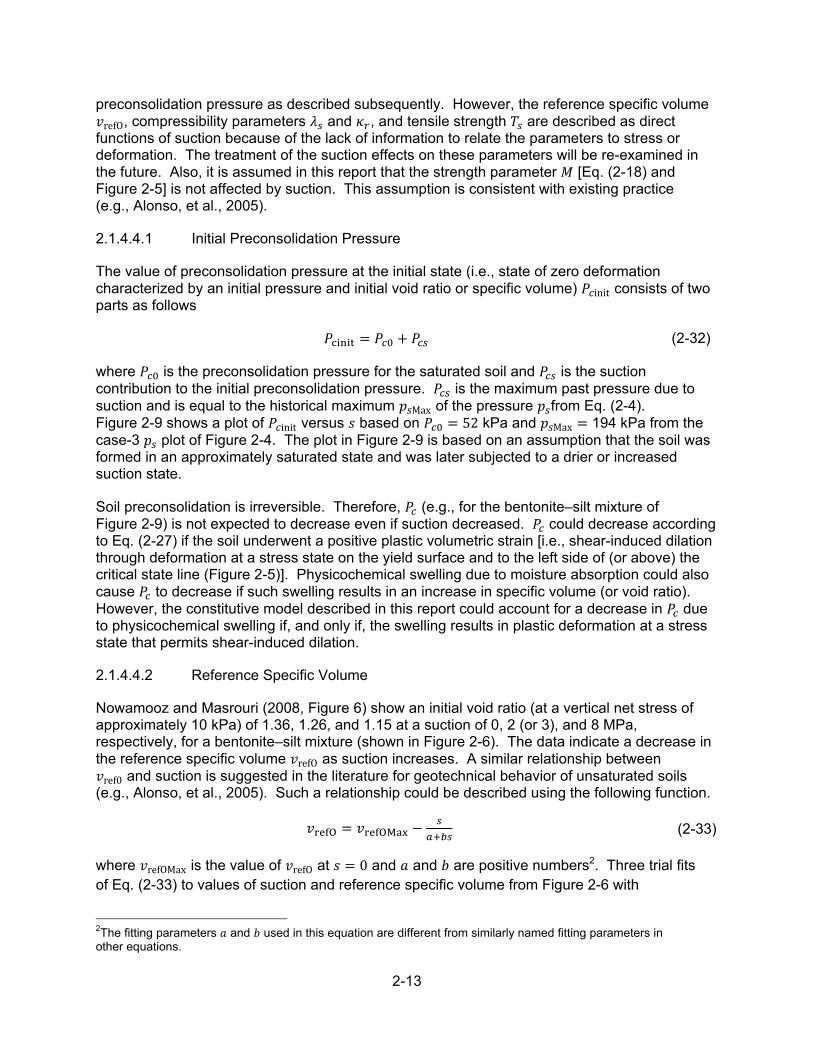
where is the preconsolidation pressure for the saturated soil and is the suction contribution to the initial preconsolidation pressure. is the maximum past pressure due to suction and is equal to the historical maximum Max of the pressure from Eq. (2-4). Figure 2-9 shows a plot of init versus based on = 52 kPa and Max = 194 kPa from the case-3 plot of Figure 2-4. The plot in Figure 2-9 is based on an assumption that the soil was formed in an approximately saturated state and was later subjected to a drier or increased suction state.

Soil preconsolidation is irreversible. Therefore, (e.g., for the bentonite–silt mixture of Figure 2-9) is not expected to decrease even if suction decreased. could decrease according to Eq. (2-27) if the soil underwent a positive plastic volumetric strain [i.e., shear-induced dilation through deformation at a stress state on the yield surface and to the left side of (or above) the critical state line (Figure 2-5)]. Physicochemical swelling due to moisture absorption could also cause to decrease if such swelling results in an increase in specific volume (or void ratio). However, the constitutive model described in this report could account for a decrease in due to physicochemical swelling if, and only if, the swelling results in plastic deformation at a stress state that permits shear-induced dilation.

2.1.4.4.2 Reference Specific Volume

Nowamooz and Masrouri (2008, Figure 6) show an initial void ratio (at a vertical net stress of approximately 10 kPa) of 1.36, 1.26, and 1.15 at a suction of 0, 2 (or 3), and 8 MPa, respectively, for a bentonite–silt mixture (shown in Figure 2-6). The data indicate a decrease in the reference specific volume refO as suction increases. A similar relationship between ref0 and suction is suggested in the literature for geotechnical behavior of unsaturated soils (e.g., Alonso, et al., 2005). Such a relationship could be described using the following function.

O = OM − (2-33)

where refOMax is the value of refO at = 0 and and are positive numbers2. Three trial fits of Eq. (2-33) to values of suction and reference specific volume from Figure 2-6 with

2The fitting parameters and used in this equation are different from similarly named fitting parameters in other equations.

2-14

Figure 2-9. Plot of Initial Preconsolidation Pressure Versus Suction for a Bentonite–Silt Mixture With = 52 kPa and = 194 kPa From Case 3 of the Plot of Figure 2-4

refOMax = 2.36 are shown in Figure 2-10. It is assumed, as Alonso, et al. (2005) suggested that

the relationship in Eq. (2-33) is reversible. Both the relationship and the reversibility assumption will be re-examined in the future.

2.1.4.4.3 Slope of the Normal-Consolidation Line

The normal consolidation line (shown schematically as AB in Figure 2-7) describes the following relationship between specific volume and pressure = N − ln for ≥ (2-34)

where A is the pressure at point A in Figure 2-7. The slope of the normal-consolidation line decreases as suction increases. The versus relationship is described as follows based on Alonso, et al. (2005) = + (1 − ) (2-35)

where max is the zero-suction value of and and are fitting parameters. Figure 2-11 illustrates the effects of (with a fixed value) on the fitted versus relationship.

2-15

Figure 2-10. Fitted Versus Relationships, Based on Figure 2-6 Data

Figure 2-11. Fitted ( ) Versus Suction ( ) Relationships, Based on Eq. (2-35) and Illustrating the Effects of the Parameter With = 0.2 and = 5 × 10−5

2-16

= O − ln for ≤ (2-36)

The slope of the recompression line appears to decrease as suction increases considering the data in Figure 2-6, for example. However, often is assumed to be independent of suction (e.g., Alonso, et al., 2005). The capability to vary with suction is included in the current model to allow an implementation of future data that may indicate dependent or independent of suction. The versus relationship is modeled as follows = − (2-37)

where max is the zero-suction value of and and are positive numbers. Figure 2-12 shows the results of fitting Eq. (2-37) to Figure 2-6 data (with “vertical net stress” modified to “effective vertical stress”).

2.1.4.4.4 An Example Set of Soil Compression Parameters

The relationships described in Sections 2.1.4.4.1 through 2.1.4.4.4 are used to generate a set of bilinear compression curves in - space for various values as shown in Figure 2-13. The relationships are used in several model verification analyses described in Section 2.3.

2.1.4.4.5 Tensile Strength

Clay soils generally have zero or negligible tensile strength when saturated but could develop a tensile strength as suction increases. Ajdari, et al. (2010), for example, show an increase in cohesion from approximately zero at saturation to approximately 150 kPa at a suction of 153 kPa for a bentonite–silt mixture. The relationship of tensile strength versus suction is represented in the model as follows to provide a capability for representing a suction-dependent tensile strength, as supported by any available data. = + (2-38)

where is the tensile strength at zero suction (often = 0) and and are positive numbers with = 1⁄ and is a maximum tensile strength. Model verification analyses described in Section 2.3 are performed using = 0, = 10, and = 25 kPa.

2.1.5 Thermal Strain

The nature of thermal strain is well explained in the following excerpt from Boley and Weiner (1997, p. 244).

Broadly speaking, thermal stresses may arise in a heated body either because of a nonuniform temperature distribution, or external constraints, or a combination of these causes. Since the effect of external constraints is readily understood, we confine our attention to that of nonuniform temperature.

Imagine a body as made up of a number of small cubical elements of equal size which fit together to form the given continuous body. If the temperature of the body is raised uniformly, and if its bounding surfaces are unrestrained, then each element will expand an equal amount (proportional to the temperature rise) uniformly in all directions. The

2-17

Figure 2-12. Fitted ( ) Versus Suction Relationships, Based on Eq. (2-37) and Figure 2-6 Data

Figure 2-13. Suction( )-Dependent Compression Curves for a Bentonite–Silt Mixture, Based on Relationships Described in Sections 2.1.4.4.1 Through 2.1.4.4.4

2-18

elements are thus still equal-sized cubes; they still fit together to form a continuous body, and no stresses arise. If, however, the temperature rise is not uniform, each element will tend to expand by a different amount that is one proportional to its own temperature rise. The resulting different-sized cubes cannot, in general, fit together; since, however, the body must remain continuous, each element must restrain the distortions of its neighbors, or, in other words, stresses must arise.

The total strains at each point of a heated body are thus made up of two parts. The first part is a uniform expansion proportional to the temperature rise . Since this expansion is the same in all directions for an isotropic body, only normal strains and no shearing strains arise in this manner. If the coefficient of linear thermal expansion is denoted by

, this normal strain in any direction is equal to .

The second part comprises the strains required to maintain the continuity of the body as well as those arising because of external loads.

Therefore, the thermal strain increment due to a temperature increment ∆ at a point in a soil medium consists of two parts. The first part is the strain due to unrestrained expansion (i.e., the expansion that would occur if the elemental volume representing the point is free to expand in every direction) and is related to ∆ as follows ∆ = (∆ ) (2-39)

where is the bulk thermal expansivity (i.e., volumetric strain increment per unit temperature increment) of the soil. This is the thermal strain increment represented in Eqs. (2-10) and (2-17). The second part is the strain needed to maintain the continuity of the body in the presence of a temperature gradient and boundary restraints. This part is not included explicitly but is calculated by satisfying the equilibrium conditions and constitutive relationships for the entire body.

Equation (2-39) defines the potential thermal strain under stress-free conditions. Therefore, the parameter α needs to be based on the thermal expansion of a soil specimen that is either completely dry or fully saturated and free draining, such that no stress or excess pore pressure develops in the specimen during testing. Because the bulk thermal expansion of a water-bearing soil element consists of the thermal expansion of the solids and water and any water drainage, as Mitchell (1976, pp. 275–281) explained, it can be shown that the bulk thermal expansivity is related as follows to the thermal expansivity of the solids and water

and the void ratio void

= +1 + − (2-40)

where DR is the volumetric drainage per unit soil volume per unit temperature increment and is the water saturation.

Thermal expansion test results that Laloui, et al. (2009) provided suggest that could be negative for a normally consolidated soil. However, as Mitchell (1976, pp. 277–278) indicated, the observed volume change during thermal-expansion testing of a water-bearing soil specimen could include the effects of excess pore-water pressure, changes in effective stress and

2-19

reduction of shear strength. Therefore, the value of determined based on the test could be misleading if such effects are significant.

Generally, the thermal expansivity of a solid is anticipated to be positive such that the volumetric strain increment in Eq. (2-39) is positive. However, the data of Laloui, et al. (2009) suggest that a temperature increment could cause contraction (instead of expansion) of an unrestrained soil element. Any thermal expansion data will need to be examined carefully to determine whether the test conditions satisfy the conditions for free expansion and free drainage. Such conditions are easier to satisfy if the specimen is either completely dry or fully saturated and free draining.

2.1.6 Physicochemically Swelling Strain

In this report, physicochemical swelling refers to the swelling of a clay soil due to an increase in water content. The strain increment associated with physicochemical swelling is represented as ∆eCW in Eqs. (2-10) and (2-17). This strain increment is the potential strain increment for an elemental soil volume (representing a point in a soil mass) that is free to expand in every direction as the water content increases. Such swelling would not result in any pressure change. However, the strain due to physicochemical swelling consists of two parts (in the same way that the strain due to thermal expansion consists of two parts as explained in Section 2.1.5). The first part is due to free swelling and is represented by ∆eCW in Eqs. (2-10) and (2-17). The second part arises from interactions due to water content gradients and boundary restraint and is not represented explicitly but results from satisfying the equilibrium conditions and constitutive relationships for the entire body.

Swelling pressure occurs if part of the potential free swelling is suppressed due to gradients in water content, mechanical properties, or boundary restraint. The potential swelling of clay soils is typically characterized using indices such as swelling potential, which is the percentage swelling (increase in volume per unit volume expressed as a percentage) from the “free-swell” test (Fredlund and Rahardjo, 1993, p. 399), or swelling pressure, which is the maximum pressure from the constant-volume swell test (e.g., Agus and Schanz, 2008). The indices were developed for comparing different soils (e.g., swelling pressure varies with clay mineralogy and chemistry and increases with dry density) or for developing empirical design parameters such as for controlling foundation heave (e.g., Fredlund and Rahardjo, 1993, p. 397).

However, for general mechanical modeling (e.g., to evaluate swelling pressure for a given waste disposal design involving a clay buffer), swelling needs to be characterized by defining the amount of free swelling that could occur at a point per a unit water content increment. Montes-H, et al. (2003) defined swelling in terms of the ratio of swelling to water adsorption (also referred to as the unit swelling potential), which equals the volumetric strain increment divided by the water content increment. The value of this ratio for free swelling conditions is adopted in this work for characterizing free swelling. That is, potential free swelling is represented by CW, such that the strain increment ∆ CW due to a water content increment ∆ is given by the following equation ∆ CW = CW(∆ ) (2-41)

Values of CW for MX80 bentonite calculated from Montes-H, et al. (2003, Figure 7), for example, are shown in Figure 2-14. The parameter CW is not usually provided with swelling information, but published measurements of swelling pressure appear abundant (e.g., Montes-H, et al., 2003; Villar and Lloret, 2004). The swelling pressure measurements

2-20

Figure 2-14. Cumulative Swelling Strain and Unit Swelling Potential for MX80 Bentonite Based on Montes-H, et al. (2003, Figure 7)

could be simulated numerically to estimate consistent values of CW if sufficient mechanical properties data are available for the tested soil.

2.2 Implementation of Constitutive Model for Use in FLAC Computer Code

The constitutive model for unsaturated soil discussed in Section 2.1 was implemented in the geomechanical simulation code FLAC Version 7.0 (Itasca, 2011). The FISH programming language embedded in FLAC is used to add a user-defined constitutive model. The user-defined model, which is called by FLAC for every solution step, uses the strain increments and stress state information from FLAC to evaluate an updated set of stresses in accordance with constitutive laws. The updated stresses are provided to FLAC for equilibrium analysis. In FLAC several FISH codes can be developed to perform specific functions and these codes can be either called from the main FLAC data file or by another FISH code. Each FISH code will be referred to as “FISH function” hereafter.

The input parameters for the constitutive model are shear modulus, ; maximum bulk modulus, ∞; slope of the critical-state line, ; reference pressure, ref; and other parameters listed in

Table 2-1. The data for these parameters are input to the model from the FLAC data file. However, as discussed in Section 2.1, several other parameters are required to define the constitutive model. A FISH function was developed to compute initial soil parameters for all zones. Some of these parameters are suction dependent, so the FISH function is also called whenever there is a change in suction. The FISH function computes the following parameters: the suction pressure, p [Eq. (2-4)], bulk modulus, K [Eq. (2-30)]; recompression slope, κ [Eq. (2-37)]; normal consolidation slope, λ [Eq. (2-35)]; tensile strength, T [Eq. (2-38)]; initial

2-21

Table 2-1. Parameters and Data Used in the Analysis

Parameters Symbols

Values (Units are for Stress in kPa and Displacement

in m)

Slope of Normal Consolidation Line

0.2 0.75 5.0 × 10−5

Slope of Swelling or Recompression

0.05 3,750 26.5

Tensile Strength 0.0

2.5 10.0

Specific Volume refOMax 2.36

2,300 4.5

Bishop’s Parameters A 500 B 0.05

Preconsolidation Pressure 5.0 or 52 kPa Shear Modulus G 250 kPa

Maximum Value of Bulk Modulus

1 × 104

Critical Slope M 1.02 Reference Pressure Ref 1.0 or 10.0

Suction s Varies: 0 To 6,000

preconsolidation pressure, P init [Eq. (2-32)]; and initial specific volume, v [Eqs. (2-33) and (2-36)].

The constitutive model uses the principle of effective stress as described in Section 2.1. An incremental algorithm of the constitutive model was developed for numerical implementation through the FISH user interface. The overall steps consist of

Calculating updated stress by adding the old stress and the elastic stress increment computed from the total strain increment

Computing the yield function using the stress invariants p and q [Eqs. (2-6) and (2-7)]

Assessing stress state with respect to the yield surface

If the stress state is elastic, returning the new stresses to FLAC

If the stress state is outside the yield surface, evaluating the plastic strain increment for calculation of the new stresses and providing to FLAC; updating specific volume, preconsolidation pressure, and bulk modulus

As discussed in Section 2.1.4.2, two approaches, one based on the consistency condition and the other using a quadratic equation, were used to evaluate the plastic strain increment. Two

2-22

implementations of the constitutive model were developed: MCUS2d using the consistency condition and MCUS2d-Q using the quadratic equation.

A number of simulation tests were conducted to verify the two implementations. The numerical tests include testing of saturated and unsaturated soil samples by simulating the oedometer test. An oedometer test is a standard laboratory test performed in geotechnical engineering to determine soil compression properties. The oedometer test simulates one-dimensional compression by applying loads to a soil sample in a rigid confining ring and measuring the vertical deformation response. The results from these tests are used to predict how a soil in the field will deform in response to a change in effective stress.

2.3 Verification and Examples

In this section numerical results are presented for the oedometer tests simulated numerically for saturated and unsaturated soil conditions. Oedometer test results are discussed for (i) saturated soil, (ii) unsaturated soil, (iii) load-path dependent unsaturated soil, and (iv) swelling of unsaturated soil.

2.3.1 Oedometer Test of Saturated Soil

The oedometer test was numerically simulated to determine stresses in a saturated soil medium. The purpose of this example is to verify the FLAC implementation of the constitutive model described in Section 2.1 by comparing calculated results against a built-in Modified CAM-Clay model in FLAC (Itasca, 2011). The FLAC built-in Modified CAM Clay model simulates nonlinearity and hardening/softening behavior of saturated soils with no resistance to tensile stress. The constitutive model for unsaturated clay soils described in Section 2.1, referred to hereafter as MCUS2d (implementation using the consistency condition) and MCUS2d-Q (implementation using the quadratic equation approach) was tested in the experimental simulation with zero values for suction (s) and tensile strength. The FLAC Modified CAM-Clay model FISH function was obtained from the FISH functions library provided with the FLAC manual.

The test was modeled using one zone (i.e., one element) of unit dimensions and in axisymmetry mode. The boundary conditions for the test are shown in Figure 2-15. The values of the input parameters used in the analysis, as discussed in Sections 2.1.4.3 and 2.1.4.4, are given in Table 2-1. An initial compressive stress state of 5 kPa was specified in x, y, and circumferential (z) directions, and the specimen was loaded through incremental downward displacement of the top boundary. The sample was subjected to several load–unload cycles. The history of Y-displacement, mean pressure, logarithm of mean pressure (ln ), and bulk modulus was monitored for the calculation steps. The results from the analyses are shown in Figures 2-16 to 2-18. The mean pressure versus Y-displacement is plotted in Figure 2-16, specific volume versus ln in Figure 2-17 and bulk modulus versus Y-displacement in Figure 2-18. In all the figures, the results obtained using MCUS2d, MCUS2d-Q, and FLAC Modified CAM Clay are plotted for comparison. The results show that

The unsaturated model and its implementation in FLAC simulates the load–unload behavior for saturated conditions satisfactorily

2-23

Figure 2-15. Boundary Conditions for Oedometer Test Model

Figure 2-16. Mean Pressure Versus Y-Displacement Comparing FLAC CAM Clay and the

Unsaturated Models

2-24

Figure 2-17. Specific Volume Versus Logarithmic of Mean Pressure Comparing FLAC

CAM Clay and the Unsaturated Models

Figure 2-18. Bulk Modulus Versus Y-Displacement Comparing FLAC CAM Clay and the Unsaturated Models

2-25

Specific volume versus ln plots in Figure 2-17 indicates both elastic and elastic–plastic conditions were encountered in the simulated tests as shown by the two sets of lines, one representing the unload–reload (i.e., elastic) behavior and the other representing the virgin compression (i.e., elastic–plastic) behavior

Unsaturated models using the consistency condition (MCUS2d) and quadratic equation (MCUS2d-Q) produce essentially identical results

All three figures show the results from MCUS2d and MCUS2d-Q models agree with results calculated using the built-in FLAC CAM Clay model

As pressure increases, results from MCUS2d and MCUS2d-Q differ more from the FLAC CAM-Clay model because of differences in the bulk modulus model

Whereas, the FLAC CAM-Clay model uses Eq. (2-29) for bulk modulus, MCUS2d and MCUS2d-Q use Eq. (2-30). The difference between Eqs. (2-29) and (2-30) increases as pressure increases and accounts for the difference between the FLAC CAM-Clay model and the other two models as shown in Figures 2-16 through 2-18.

2.3.2 Oedometer Test of Unsaturated Soil

The MCUS2d implementation of the unsaturated soil model was used to study the effect of saturation on the compression behavior of an oedometer test specimen. The model geometry and the boundary conditions as described in Section 2.3.1 were used in the analysis. For the simulated tests, the specimen was loaded axially in compression for a higher loading range than in Section 2.3.1 to induce inelastic behavior in the specimen. The onset of virgin compression (inelastic) behavior occurred at higher pressure because of the increased preconsolidation pressure at higher suction as described in Section 2.1.4.4.1 and Figure 2-9. The input data for the soil used in the analysis are described in Sections 2.1.4.3 and 2.1.4.4 and given in Table 2-1. Tests were simulated for constant suction for six different suction values ( = 0, 10, 100, 600, 2,500 and 6,000 kPa), and all specimens were compressed to the same vertical displacement. The suction values were chosen to represent a sample range in suction versus effective stress plot in Figure 2-4 (Case 3). As shown in Figure 2-4, the peak value of suction pressure occurs at approximately a suction of 600 kPa. Thus, the chosen suction values represent two values on the steep part of the rising curve (10 and 100 kPa) and two values on the asymptotic decline part of the curve (2,500 and 6,000 kPa). Tests for suction values of 0 and 600 kPa were also performed. The value of suction for each test was applied as a prescribed input.

The results from the model simulation for all suction values are presented in three plots: (i) mean pressure versus Y-displacement in Figure 2-19, (ii) bulk modulus versus Y-displacement in Figure 2-20, and (iii) specific volume versus effective pressure in log scale in Figure 2-21. All test results show elastic and elastic–plastic deformation responses. The calculated responses for the various suction values are related to each other in a way consistent with the input data. For example, the calculated specific volume versus effective pressure relationships in Figure 2-21 are consistent with the input specific volume versus effective pressure relationships in Figure 2-13. The two figures can be compared by examining the value of specific volume at the reference effective pressure (10 kPa) for the cases that include a pressure of 10 kPa, the values of preconsolidation pressure (intersection of the reloading line with the virgin–compression line), and the value of specific volume at any arbitrary pressure included in the calculated result. The calculation for each non-zero suction case has to begin at

2-26

Figure 2-19. Mean Total Pressure Versus Y-Displacement for Different Suction Values in kPa

Figure 2-20. Bulk Modulus Versus Y-Displacement for Different Suction Values in kPa

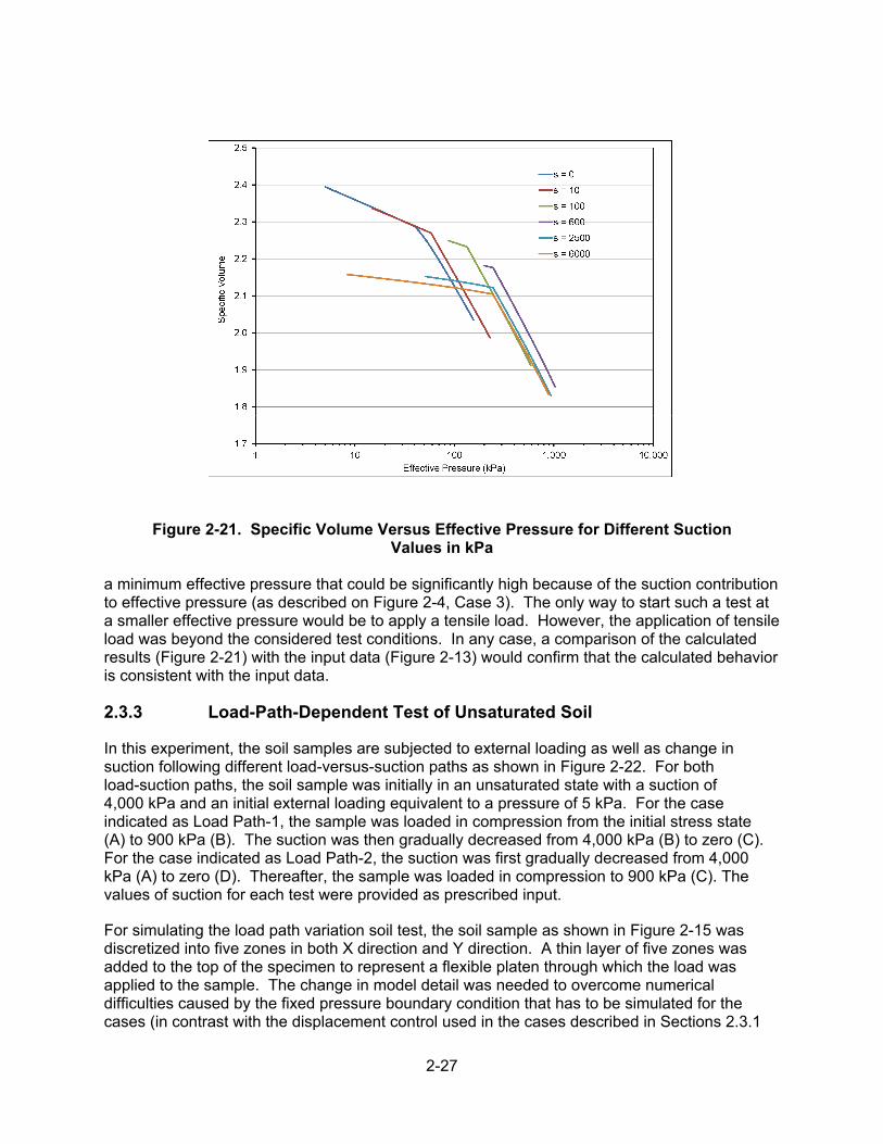
2-27

Figure 2-21. Specific Volume Versus Effective Pressure for Different Suction Values in kPa

a minimum effective pressure that could be significantly high because of the suction contribution to effective pressure (as described on Figure 2-4, Case 3). The only way to start such a test at a smaller effective pressure would be to apply a tensile load. However, the application of tensile load was beyond the considered test conditions. In any case, a comparison of the calculated results (Figure 2-21) with the input data (Figure 2-13) would confirm that the calculated behavior is consistent with the input data.

2.3.3 Load-Path-Dependent Test of Unsaturated Soil

In this experiment, the soil samples are subjected to external loading as well as change in suction following different load-versus-suction paths as shown in Figure 2-22. For both load-suction paths, the soil sample was initially in an unsaturated state with a suction of 4,000 kPa and an initial external loading equivalent to a pressure of 5 kPa. For the case indicated as Load Path-1, the sample was loaded in compression from the initial stress state (A) to 900 kPa (B). The suction was then gradually decreased from 4,000 kPa (B) to zero (C). For the case indicated as Load Path-2, the suction was first gradually decreased from 4,000 kPa (A) to zero (D). Thereafter, the sample was loaded in compression to 900 kPa (C). The values of suction for each test were provided as prescribed input.

For simulating the load path variation soil test, the soil sample as shown in Figure 2-15 was discretized into five zones in both X direction and Y direction. A thin layer of five zones was added to the top of the specimen to represent a flexible platen through which the load was applied to the sample. The change in model detail was needed to overcome numerical difficulties caused by the fixed pressure boundary condition that has to be simulated for the cases (in contrast with the displacement control used in the cases described in Sections 2.3.1

2-28

Figure 2-22. Load Path for Unsaturated Soil Test

and 2.3.2). The interface between the platen and soil were assumed to be bonded. In Load Path-1 the loading of the sample was controlled by displacement where a constant velocity was applied to the platen at 5 × 10−6 m/step. At the end of the loading cycle, when the pressure in the specimen reached 900 kPa, the velocity boundary condition was removed and replaced by an equivalent pressure on the platen. The suction was then gradually decreased in steps of 20 kPa, and at each suction step the sample was cycled to equilibrium. For Load Path-2, a similar approach was used where the suction was reduced in steps and the sample was loaded vertically.

The results for Load Path-1 are shown in Figure 2-23. The figure shows specific volume versus total pressure in log scale. The loading points A, B, and C are marked on the figure. The curve A-B depicts a bilinear behavior indicating initial elastic deformation until about 250 kPa where the specific volume decreased from 2.15 to 2.1, followed by a sharp decrease in specific volume to 1.84 indicating inelastic deformation till the end of loading. At point B when the suction was decreased from 4,000 kPa to zero, the specific volume initially increased from 1.84 to 1.855 and then decreased to about 1.82. The response of the specimen to suction in the high stress regime is consistent with Figure 2-13, which shows that, starting from a high suction value (4,000 kPa), the soil–specific volume would increase initially with decreasing suction to a suction of approximately 500 kPa; thereafter, the specific volume would decrease as suction decreases toward zero. The calculated results for Load Path-2 (Figure 2-24) show the specific volume increased from about 2.15 (A) to 2.3 (D) when the suction was decreased. The trend is consistent with Figure 2-13, which shows that at low effective stress the specific volume increases with a decrease in suction. Subsequent loading path D to C shows elastic and plastic deformation and the specific volume is about 1.68 when the total pressure is about 900 kPa.

2.3.4 Swelling Example

A series of simulated oedometer tests were performed to examine swelling pressure development in a confined swelling clay soil. The specimen setup described in Figure 2-15 was

2-29

Figure 2-23. Specific Volume Versus Total Pressure for Load Path−1

Figure 2-24. Specific Volume Versus Total Pressure for Load Path−2

2-30

modified by replacing the top boundary condition with a no-displacement boundary (i.e., the specimen was fully constrained and could not deform). The initial suction was set to 4,000 kPa. Then suction was decreased to zero in 20-kPa steps. The specimen water content corresponding to each suction value was calculated by assuming = where is the effective saturation [Eq. (2-5)] and χ was calculated using Figure 2-3 (Case 3). The swelling strain due to the water content change for each step was calculated using Eq. (2-41) and applied to the constitutive model as described in Section 2.1 [see Eq. (2-17)]. The specimen loading condition was cycled to establish equilibrium at each step. The calculated swelling pressure is shown in Figure 2-25 as a function of water content for four different values of the unit swelling potential parameter αCW [Eq. (2-41)].

This example illustrates using the constitutive model for swelling and swelling pressure analysis. However, the specific numerical values calculated are not to be associated with any real situation, because the parameter set used is likely inconsistent. As described in Section 2.1.4, several mechanical parameters were evaluated by curve-fitting data from Figure 2-6 and others from the literature. Furthermore, the moisture content versus suction behavior was not based on a moisture characteristic curve but was derived from a versus relationship based on curve-fitting literature data. The authors expect to perform more calculations using the model with consistent parameters for a characterized soil.

2.4 Future Work

As described in Sections 2.2 and 2.4, the constitutive model described in Section 2.1 is developed enough and implemented to be used to model the mechanical behavior of unsaturated/saturated expansive clay soil as a part of an engineered structure or natural geologic medium. However, the model needs to be improved in several ways to enhance the capabilities.

Implement the model for FLAC3D. The current implementation is for FLAC, which is limited to two-dimensional and one-dimensional geometries. FLAC3D can be used for one-, two-, or three-dimensional geometry.

Develop control functions to enable sequential dynamic coupling of mechanical analyses using FLAC3D and thermal-hydrological analyses using xFlo as described in Chapter 4.

Perform analyses to explore and illustrate the capabilities of the constitutive model, including structures with one-, two-, and three-dimensional geometries; spatially and temporally variable moisture and temperature gradients; and unit swelling potential.

Use the model with the controlling functions (described in the second bulleted item) to model the DECOVALEX task described in Chapter 1.

2-31

Figure 2-25. Swelling Pressure Versus Water Content for Four Different Values Swelling Potential Parameter, CW

3-1

3 MODELING THERMOHYDROLOGICAL PROCESSES USING xFlo

Coupled thermohydrological (TH) numerical models are useful tools for understanding relative importance, competition, and dynamic interactions of multiphase processes in evaluating suitability of potential geological repositories for high-level nuclear waste disposal. xFlo (Version 1.0β) is an in-house TH model (Painter, 2006), that was built on its predecessor coupled-process simulator, known as MULTIFLO (Lichtner, 1996; Painter and Seth, 2003). xFlo was recently parallelized for computationally efficient simulations by implementing domain decomposition parallelization with one-sided message passing interface communication (Başağaoğlu, et al., 2011).

Built-in unstructured grid design in xFlo provides flexibility in simulating geometrically complex flow domains. Moreover, the modular structure of xFlo allows new physical models (e.g., mechanical processes) to be added or externally coupled without changing the underlying numerical infrastructure and solvers. Therefore, xFlo is chosen as a TH simulator for the planned coupled thermohydrological-mechanical (THM) simulations as part of the ongoing Integrated Spent Nuclear Fuel Project.

The following description supplements the xFlo user’s manual (Painter, 2006) by documenting constitutive relationships provided in xFlo. The constitutive relationships in xFlo were selected using the scientific literature augmented by professional judgment. The modular format of the code allows additional relationships to be included as needed.

3.1 Description of xFlo

xFlo is a continuum-scale, multiphase TH model that can be used to simulate variably saturated flows in fractured-porous domains under transient thermal loadings. xFlo simulates the fluid in three distinct phase states—two-phase, all-gas, and no-gas conditions—by solving coupled sets of mass-balance Eq. (3-1) and heat-balance Eq. (3-2) equations

, = − ∙ + +, (3-1)

+ (1 − ), = − ∙ ℎ + ∙ [ ] +, (3-2)

in which subscript = , represents air or water; subscript = , represents liquid and gas phases; is porosity [-]; is molar mass fraction [-]; is the phase density on a molar basis [mol/m3]; is the phase saturation [-]; is the Darcy velocity [m/s]; the effective diffusion coefficient [m2/s]; is the mass source rate [mol/m3-s]; u is the internal energy [J/mol]; is the density of the mineral solid [kg/m3]; is heat capacity of the mineral solid [J/K-kg]; ℎ is the enthalpy [J/mol]; is the effective thermal conductivity [W/m-K]; is the energy source rate [J/m-K]; T is temperature [K]; and t is time [s].

3-2

In numerical simulations, the flow domain is divided into a set of unstructured grid elements with arbitrary interelement connectivity. Each grid element is described by

Volume [m3] x-, y-, and z-coordinates [m] for nodes Node number of its neighboring grid elements[-] Connection number to its neighboring grid elements [-] Distance from its center to neighboring grid element boundaries [m] Surface area connection between neighboring elements [m2]

Equations (3-1) and (3-2) are solved for fluid-state-dependent primary variables (Table 3-1) for each grid element in each timestep. In the solution phase, Eqs. (3-1) and (3-2) are discretized in space using the integral finite-difference method. Timestepping is implicit. Newton-Raphson iteration is used to solve nonlinear terms, in which the Jacobian matrix is numerically constructed via the perturbation method.

In numerical simulations, xFlo allows phase changes in each grid element. Conditions that trigger phase changes are listed in Table 3-2. These conditions are checked for each grid element in each timestep. If the conditions are met at the particular grid element, a phase change is implemented and the list of primary variables is updated in accordance with Table 3-1. Table 3-2 shows that xFlo does not allow phase changes from an all-gas phase to a no-gas phase and vice versa.

In Table 3-2, is the saturated vapor pressure [Pa]. In xFlo, it is expressed empirically as a function of system temperature and a user-specified reference temperature, ref [ ]

If < ref, = 10 . . (3-3)

If T≥Tref, PSV=10-102898T2 -1606.62T +10.047763

(3-4)

A reference temperature value, ref of 273.15 K, is hard-wired in xFlo and the same value is consistently used in all constitutive relations in the code. Eqs. (3-3) and (3-4) are the fitted empirical relations to temperature versus saturated vapor pressure data from the National Institute of Standards and Technology (NIST) Steam Table (NIST, 2011) or any output tables derived from the NIST Steam Table (e.g., http://enpub.fulton.asu.edu/ece340/pdf/steam_tables.PDF). In xFlo, water vapor pressure is assumed to be in equilibrium with the liquid phase. Hence, the vapor pressure follows the saturated vapor pressure. Therefore, the total gas pressure is expressed as = + (3-5)

in which is the air partial pressure. , , and , in Table 3-1 are the molar fraction of water in gas, air in liquid, and air in gas and they are computed as = ⁄ (3-6)

3-3

Table 3-1. Primary Variables for Each Fluid State State of the System Primary Variables

Two-phase condition S , , All-gas condition , , No-gas condition , ,

Table 3-2. Specific Conditions Implemented in xFlo Code for Phase Transitions Phases Two Phase All Gas No Gas

Two phase — ≥ 1 ≤ All gas ≥ — — No gas ≥ — — = − (3-7) = 1 − (3-8)

in which is the Henry’s constant [-].

3.2 Constitutive Relations for Unsaturated Flow Simulations

In two-phase regions of an xFlo simulation domain, relations between capillary pressure and relative permeability of the flow domain as a function of effective liquid saturation are specified using van Genuchten relations. Effective liquid phase saturation, , is computed from = ( − ) (1 − )⁄ (3-9)

in which is the liquid phase saturation [-] and is the residual liquid phase saturation [-]. Relative permeability of the liquid phase, , [-], is computed from van Genuchten relations using the Mualem model (van Genuchten, 1980) as a function of

If < ∗, then , = 1 − 1 − ( ) / (3-10)

If > ∗, then , = 1 + [ + (1 − )](1 − ) (3-11)

in which , , and are the fitting parameters and ∗ is a user-specified transition saturation [-] indicating that the cells are nearly saturated. Relative permeability for the gas phase is defined by

, = 1 − , (3-12)

The capillary pressure, [Pa], is computed from van Genuchten relations as a function of S using the first assumption for integration of the incomplete beta function in van Genuchten (1980):

3-4

If min < ≤ ∗, then = 1 ( ) − 1 (3-13)

If ∗ < < 1, then = 1 [ + (1 − )(1 − )] (3-14)

If ≥ 1, then = 0 (3-15)

If ≤ min, then = 1 ( min) + −(1 − ) ( min)( min) − 1 ( − min) (3-16)

in which , , and α are fitting parameters.

In xFlo, the user specifies van Genuchten curves to describe the capillary pressure and relative permeability relationships. A single van Genuchten curve in xFlo is defined by nine parameters

, , , min, ∗, , , , and . A curve can be assigned to a particular grid element or to a set of grid elements in numerical simulations, with as many curves defined as necessary to describe all grid elements. In two-phase zones, the liquid pressure is computed using the identity = − (3-17)

after the capillary pressure is computed from Eqs. (3-13) through (3-16).

3.3 Calculation of Fluid Properties

xFlo calculates the following fluid properties in each timestep:

Molar density of the liquid phase, [mol/m3], and the molar density of the gas phase, [mol/m3]

= 1 + − 10

(3-18)

= ( )⁄ (3-19)

in which R is the ideal (universal) gas constant (8.314 [J/K]), is the isothermal compressibility (5·10-10 [Pa−1]); is the molecular weight of water (0.0180153 kg/mol); and ρ is the density of pure water at 4 °C (1,000 kg/m3). Eq. 3-18 is from the legacy code MULTIFLO and we are currently investigating its technical basis. In the current version of xFlo, thermal expansion of water is not considered. However, we plan to include the effects of thermal expansion of water on pore water pressure in xFlo.

Dynamic viscosity of the liquid phase, [Pa-s]

Dynamic viscosity depends on a crossover (threshold) temperature, Cross (internally set to 20 K in xFlo), and the reference temperature, ref (Lide, 1986)

3-5

Crit = max ( − Ref), (−70) (3-20) If ( Crit < Cross) then = 13.01998.333 + 8.1855( Crit − Cross) + 0.00585( Crit − Cross) + 13.01998.333

(3-21)

If ( Crit ≥ Cross) then = 132.72( Crit − Cross) − 0.00001053( Crit − Cross)Crit + 105

(3-22)

Viscosity of the gas phase, [Pa-s] based on Sutherland’s formula and the Wilke formula (Kee, et al., 2003)

= 1.51175 ∙ 10 /+ 125.262

(3-23)

= 1.75528 ∙ 10 /+ 620.992 (3-24)

= ++

(3-25)

= 1 +8 1 +

(3-26)

= 1 +8 1 +

(3-27)

= 1 − (3-28)

in which is the molecular weight of dry air, which is set to 0.028964 kg/mol in xFlo.

Energy density of gas and liquid phases, [J/mol] and U [J/mol] = 76( − ref) (3-29) = + (3-30)

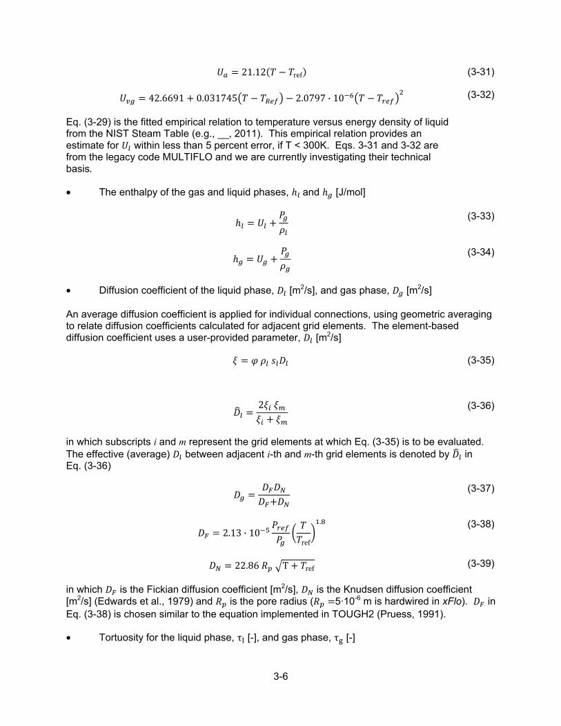
3-6

= 21.12( − ref) (3-31) = 42.6691 + 0.031745 − − 2.0797 ∙ 10 −

Eq. (3-29) is the fitted empirical relation to temperature versus energy density of liquid from the NIST Steam Table (e.g., __, 2011). This empirical relation provides an estimate for within less than 5 percent error, if T < 300K. Eqs. 3-31 and 3-32 are from the legacy code MULTIFLO and we are currently investigating their technical basis.

(3-32)

The enthalpy of the gas and liquid phases, ℎ and ℎ [J/mol]

ℎ = + (3-33)

ℎ = + (3-34)

Diffusion coefficient of the liquid phase, [m2/s], and gas phase, [m2/s]

An average diffusion coefficient is applied for individual connections, using geometric averaging to relate diffusion coefficients calculated for adjacent grid elements. The element-based diffusion coefficient uses a user-provided parameter, [m2/s] = (3-35)

= 2 + (3-36)

in which subscripts i and m represent the grid elements at which Eq. (3-35) is to be evaluated. The effective (average) between adjacent i-th and m-th grid elements is denoted by in Eq. (3-36)

= + (3-37)

= 2.13 ∙ 10 ref.

(3-38)

= 22.86 T + ref (3-39)

in which is the Fickian diffusion coefficient [m2/s], is the Knudsen diffusion coefficient [m2/s] (Edwards et al., 1979) and is the pore radius ( =5·10-6 m is hardwired in xFlo). in Eq. (3-38) is chosen similar to the equation implemented in TOUGH2 (Pruess, 1991).

Tortuosity for the liquid phase, τ [-], and gas phase, τ [-]

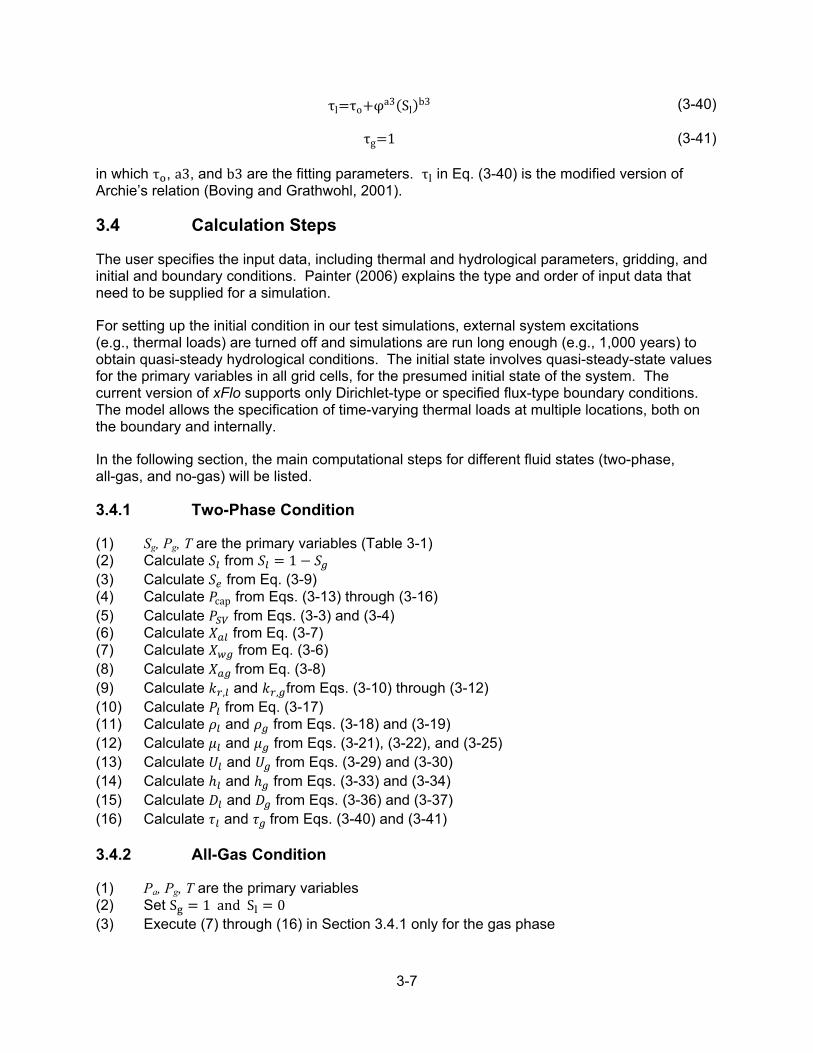
3-7

τl=τo+φa3(Sl)b3 (3-40) τg=1 (3-41)

in which τ , a3, and b3 are the fitting parameters. τ in Eq. (3-40) is the modified version of Archie’s relation (Boving and Grathwohl, 2001).

3.4 Calculation Steps

The user specifies the input data, including thermal and hydrological parameters, gridding, and initial and boundary conditions. Painter (2006) explains the type and order of input data that need to be supplied for a simulation.

For setting up the initial condition in our test simulations, external system excitations (e.g., thermal loads) are turned off and simulations are run long enough (e.g., 1,000 years) to obtain quasi-steady hydrological conditions. The initial state involves quasi-steady-state values for the primary variables in all grid cells, for the presumed initial state of the system. The current version of xFlo supports only Dirichlet-type or specified flux-type boundary conditions. The model allows the specification of time-varying thermal loads at multiple locations, both on the boundary and internally.

In the following section, the main computational steps for different fluid states (two-phase, all-gas, and no-gas) will be listed.

3.4.1 Two-Phase Condition

(1) Sg, Pg, T are the primary variables (Table 3-1) (2) Calculate from = 1 − (3) Calculate from Eq. (3-9) (4) Calculate cap from Eqs. (3-13) through (3-16) (5) Calculate from Eqs. (3-3) and (3-4) (6) Calculate from Eq. (3-7) (7) Calculate from Eq. (3-6) (8) Calculate from Eq. (3-8) (9) Calculate , and , from Eqs. (3-10) through (3-12) (10) Calculate from Eq. (3-17) (11) Calculate and from Eqs. (3-18) and (3-19) (12) Calculate and from Eqs. (3-21), (3-22), and (3-25) (13) Calculate and from Eqs. (3-29) and (3-30) (14) Calculate ℎ and ℎ from Eqs. (3-33) and (3-34) (15) Calculate and from Eqs. (3-36) and (3-37) (16) Calculate and from Eqs. (3-40) and (3-41)

3.4.2 All-Gas Condition

(1) Pa, Pg, T are the primary variables (2) Set S = 1 and S = 0 (3) Execute (7) through (16) in Section 3.4.1 only for the gas phase

3-8

3.4.3 No-Gas Condition

(1) Xal, Pl, T are the primary variables (2) Set = 0 and = 1 (3) Calculate from Eqs. (3-3) and (3-4) (4) Execute (9) and Eqs. (11) through (16) from Section 3.4.1 only for the liquid phase

3.5 Calculation of Secondary (Flux) Terms

After primary variables (Table 3-1) are calculated, secondary (derived variables), including mass and flux terms are computed. xFlo calculates air mass, [mol]; the total air and water mass,

[mol]; and energy content, [J] in each timestep from = + (3-42) = + (3-43) = + ( ) + (1 − ) (3-44)

in which is the specific heat of the rock [J/kg-K] and V is the volume of a grid element [m3].

Next, xFlo calculates dissolved air flux, air and water flux, and energy flux across the boundaries of adjacent grid elements of and . The model first calculates the average fluid density, [mol/m3], between two adjacent elements; hydraulic potential difference, ∆Θ [Pa]; mobility [mol/( m3 Pa·s)]; and average transmissibility, [m3] between grid elements of m and i = [ ( ) + ( )] 2⁄ (3-45) ∆ = [ ( ) − ( )] + [ ( ) − ( )] (3-46) = ( , ) , ⁄ (3-47) = ( ) ( ) ( ) ( ) + ( ) ( )⁄ (3-48)

in Eq. (3-46) is calculated at the upstream grid elements [i.e., at the grid element with a larger ( + )]. ( ) and ( ) are the distance from the center of a grid element to the boundary of the i-th and m-th element [m]. Permeabilities, and [m2] in Eq. (3-48), are input parameters. After Eqs. (3-45) through (3-48) are calculated, xFlo calculates air flux, [mol/s], the total flux of air and water, [mol/s], and energy (heat) flux, [J/s], as follows = ∆ (3-49) = ∆ (3-50) = ∆ ℎ ( , ) (3-51)

For both the mass fraction of air in liquid, , and the liquid phase enthalpy, ℎ , the value in upstream grid cell is used for the flux calculation.

3-9

3.6 Porosity-Dependent Parameters and Processes

xFlo (Version 1.0β) assumes that porosity remains unchanged during TH processes. When xFlo is integrated or externally coupled with a mechanical model to simulate coupled THM processes in a geological medium, the assumption of a constant porosity may not be valid if the geological medium deforms under mechanical and/or thermal stress. Therefore, in such simulations temporal variations in porosity should be accommodated in THM models.

At present, updated porosity values are directly considered in calculating , , and , . Parameters depending on these values, such as , , indirectly account for updated porosity values. Temporal change in due to changes in porosity will have direct impacts on the effective diffusion rate of the liquid phase via Eq. (3-36). The main motive for considering the porosity-dependent changes in and , is that as the porosity of the geological medium changes, liquid saturation in pore spaces would change, which would alter , . Changes in the liquid saturation would also alter the balance between the air and liquid pressures, and hence, cap would be altered [Eq. (3-17)].

3.7 Future Tasks

Test xFlo with two- and three-dimensional hypothetical TH problems

Test xFlo with TH experimental (laboratory and field) data, which will be acquired from HE-D and HE-E experiment, as part of DECOVALEX Task B1 discussed in Section 1.2

3.8 Potential Improvements on xFlo

The current version of the xFlo does not accommodate

Hysteresis in wetting and draining cycles in water retention characteristics of the geological medium

Liquid saturation versus relative permeability or liquid saturation versus capillary pressure input in a tabular format (currently, the user is required to provide a set of van Genuchten parameters instead)

Anisotropy in thermal conductivity and permeability

These are some modeling features that should be included in xFlo to improve flexibility and enhance accuracy in numerical simulations of experimental and field data. These features are planned to be implemented in the xFlo code in future.

4-1

4 COUPLING THERMOHYDROLOGICAL AND MECHANICAL MODELS

An external coupling and joint execution of a TH model (xFlo) and a mechanical model (FLAC3D) is underway for development of a THM simulator for nonisothermal, multiphase flows in deformable fractured-porous media. The coupled model is intended to be used for performance evaluation of processes in the near-field environment for geological disposal of high-level radioactive waste.

4.1 Coupling of xFlo and FLAC3D

The main objective of this modeling effort is to develop a fully coupled THM model, in which xFlo and FLAC3D will be linked externally while synchronizing information exchange between them at every timestep through a master code. Although FLAC3D will be used in the subsequent sections in referring to the mechanical model, we first plan to externally link xFlo to FLAC and test the performance of the coupled model with one- and two-dimensional problems.

At present, both xFlo and FLAC are semi-THM models in the sense that xFlo runs as a stand-alone code with a user-supplied time series of rock porosity, and similarly, FLAC runs as a stand-alone code with user-supplied time series of hydrologic properties.

For a successful dynamic coupling of xFlo and FLAC (or FLAC3D)

A grid structure of a flow domain needs to be compatible with both models

The assignment of system parameters and variables to each grid element needs to be consistent in both models

Two-way information exchange between these models needs to occur dynamically

When xFlo and FLAC3D are fully coupled, the grid structure of a flow domain will be constructed by FLAC3D and then passed to xFlo, because xFlo has the flexibility for handling an unstructured grid network with arbitrary inter-element connectivity. Therefore, all calculations will be performed on the same grid layout both in xFlo and FLAC3D. For xFlo to work with the same grid structure, FLAC3D will provide information so that each grid element can be registered by (i) its volume [m3]; (ii) its x-, y-, and z-coordinates [m]; (iii) the node number of its neighboring elements [-]; (iv) connection number to its neighboring elements [-]; (v) the distance from its center to neighboring element boundaries [m]; and (vi) the surface area connection between neighboring elements [m2].

A schematic displaying information exchanges between xFlo and FLAC3D is shown in Figure 4-1. The coupling of xFlo and FLAC3D proposed in this work will be similar to the coupling of FLAC3D and TOUGH2 in Rutqvist et al. (2002). The mechanical model associated with FLAC3D is discussed in Chapter 2. State equations relevant to xFlo are discussed in Chapter 3. Selected model parameters are listed in Appendix C. In xFlo, hydrological and thermal parameters and computed primary and secondary variables (as discussed in Chapter 3) are assigned to the center of each grid element (i.e., block-centered specification) and these properties and variables presumably remain uniform across each element. Similarly, FLAC3D assigns system parameters and computed system variables at the center of each grid element, except for displacements computed internally at the corner of each grid element. However, xFlo does not use these nodal displacements. Instead, block-centered porosities computed based on the specific volume calculated by the mechanical model via Eqs. (2-11) through (2-13) will be

4-2

Figure 4-1. A Schematic Demonstrating xFlo and FLAC3D Coupling

passed to xFlo. Hence, xFlo and FLAC3D will exchange only block-centered parameters and variables in each timestep.

After a grid structure is constructed by FLAC3D and communicated to xFlo and initial and boundary conditions are implemented for the TH and mechanical components of the problem, FLAC3D calculates block-centered porosities for a given initial thermal and hydrological state of the flow domain. xFlo then calculates all primary and secondary variables as functions of new porosities. These calculations have adopted corrections due to new porosities on relative permeability of the liquid phase, , , and capillary pressure, Pcap, as suggested by Rutqvist, et al. (2002)

, = , ( ) (4-1)

cap = cap( ) , ( )⁄, ⁄ (4-2)

in which represents the initial porosity and is the fitting parameter. As discussed in Section 3-6, the main motive for considering porosity-dependent changes in cap and , is that as the porosity of a deformable geological medium changes, liquid saturation in pore spaces would change, which would alter , . Changes in the liquid saturation would also alter the balance between the air and liquid pressures, and hence, would be altered. Moreover, tortuosity for the liquid phase, , in xFlo is recalculated in each timestep as a function of time-varying porosity via Eq. (3-37).

Based on new porosities, xFlo then calculates the gas pressure, Pg; liquid pressure, Pl; capillary pressure, Pcap; temperature, T; and liquid saturations, Sl for each element. This information

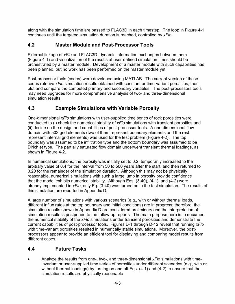
4-3

along with the simulation time are passed to FLAC3D in each timestep. The loop in Figure 4-1 continues until the targeted simulation duration is reached, controlled by xFlo.

4.2 Master Module and Post-Processor Tools

External linkage of xFlo and FLAC3D, dynamic information exchanges between them (Figure 4-1) and visualization of the results at user-defined simulation times should be orchestrated by a master module. Development of a master module with such capabilities has been planned, but no work has been performed on the master module yet.

Post-processor tools (codes) were developed using MATLAB. The current version of these codes retrieve xFlo simulation results obtained with constant or time-variant porosities, then plot and compare the computed primary and secondary variables. The post-processors tools may need upgrades for more comprehensive analysis of two- and three-dimensional simulation results.

4.3 Example Simulations with Variable Porosity

One-dimensional xFlo simulations with user-supplied time series of rock porosities were conducted to (i) check the numerical stability of xFlo simulations with transient porosities and (ii) decide on the design and capabilities of post-processor tools. A one-dimensional flow domain with 502 grid elements (two of them represent boundary elements and the rest represent internal grid elements) was used for the test problem (Figure 4-2). The top boundary was assumed to be infiltration type and the bottom boundary was assumed to be Dirichlet type. The partially saturated flow domain underwent transient thermal loadings, as shown in Figure 4-2.

In numerical simulations, the porosity was initially set to 0.2, temporarily increased to the arbitrary value of 0.4 for the interval from 50 to 500 years after the start, and then returned to 0.20 for the remainder of the simulation duration. Although this may not be physically reasonable, numerical simulations with such a large jump in porosity provide confidence that the model exhibits numerical stability. Although Eqs. (3-40), (4-1), and (4-2) were already implemented in xFlo, only Eq. (3-40) was turned on in the test simulation. The results of this simulation are reported in Appendix D.

A large number of simulations with various scenarios (e.g., with or without thermal loads, different influx rates at the top boundary and initial conditions) are in progress; therefore, the simulation results shown in Appendix D are considered preliminary and the interpretation of simulation results is postponed to the follow-up reports. The main purpose here is to document the numerical stability of the xFlo simulations under transient porosities and demonstrate the current capabilities of post-processor tools. Figures D-1 through D-12 reveal that running xFlo with time-variant porosities resulted in numerically stable simulations. Moreover, the post-processors appear to provide an efficient tool for displaying and comparing model results from different cases.

4.4 Future Tasks

Analyze the results from one-, two-, and three-dimensional xFlo simulations with time-invariant or user-supplied time series of porosities under different scenarios (e.g., with or without thermal loadings) by turning on and off Eqs. (4-1) and (4-2) to ensure that the simulation results are physically reasonable

4-4

Test whether the FLAC3D-constructed grid structure is correctly communicated to xFlo

Design and develop a master model that will externally link xFlo and FLAC3D

Test the performance of the coupled model with one-, two-, and three-dimensional hypothetical data for a complete THM simulation

Test the performance of the coupled model with a complete set of THM experimental data from the HE-D and HE-E experiments

Figure 4-2. One-Dimensional Flow Domain Geometry and the Thermal Loading Applied to the Flow Domain in the Test Simulation

5-1

5 SUMMARY

This report focused on coupled processes associated with emplacement of waste in deep underground facilities. This is the second report related to work performed under the coupled processes topic, under the Integrated Spent Fuel Program. Initial stages in the development of the numerical modeling approach to couple thermohydrological processes (using xFlo) with geomechanical processes (using FLAC) was the focus of this report. The immediate purpose of numerical code development was to support U.S. Nuclear Regulatory Commission–Center for Nuclear Waste Regulatory Analyses (NRC–CNWRA®) participation in the Development of Coupled models and their VALidation against Experiments (DECOVALEX) program. Much of the information in this report was presented and discussed in the joint NRC–CNWRA Coupled Processes workshop held on June 27, 2012.

The current phase of DECOVALEX, D-2015, was initiated in April 2012 and will extend until November 2015. Modeling the thermohydrological-mechanical (THM) processes at the heater test (HE-E) at Mont Terri, Switzerland was chosen as the main task CNWRA staff to support NRC staff in D-2015. The HE-E test focuses on the THM behavior of the buffer and its interaction with the host rock during the early postclosure period when the waste is emplaced. The processes of drying and subsequent resaturation of the buffer influence its swelling capacity. The modeling of the HE-E test has been divided into four steps: (i) host rock characterization, (ii) buffer characterization, (iii) HE-E model development, and (iv) HE-E model calibration. NRC staff may also be involved in other tasks such as SEALEX test and THMC modeling of a single fracture. The SEALEX test focuses on hydromechanical processes important for long-term performance of bentonite sealing plugs for horizontal emplacement boreholes in an argillite host rock. The four phases for the SEALEX test under D-2015 are (i) characterize bentonite–sand properties using laboratory data; (ii) simulate a laboratory scale mockup experiment; (iii) simulate in-situ water loss to the host rock (i.e., Toarcian Argillites); and (iv) simulate conditions in two large-scale in-situ sealing experiments. The THMC processes in a single fracture task in D-2015 focuses on changes in hydraulic properties caused by mechanical closing of fracture apertures and mineral dissolution and precipitation under applied mechanical stress and various thermal conditions.

Chapter 2 described the development and numerical implementation of a constitutive model for the mechanical behavior of unsaturated expansive clay soils. The constitutive model is based on combining stresses due to suction and external loading using the principle of effective stress and deriving stress strain relationships based on elastoplasticity theory and procedures. The resulting constitutive model can be implemented in any existing geomechanics modeling code that provides an interface for implementing user-defined material models, such as FLAC. Deformation due to external loading, thermal expansion, and chemically assisted swelling due to moisture absorption is accounted for in the constitutive model. The constitutive model was implemented in the geomechanical simulation code FLAC Version 7.0 through the FISH function user interface. The implementation was verified using hypothetical test problems and the verification analyses gave satisfactory results. Additional verification analyses using laboratory data and information from literature are planned for the next fiscal year. Planned work for improving modeling capabilities include (i) implementation in FLAC3D that extends modeling capability to three-dimensional geometry and (ii) performing analyses to explore and illustrate the capabilities of the constitutive model, including modeling structures with one-, two-, and three-dimensional geometries spatially and temporally variable moisture and temperature gradients and unit swelling potential.

5-2

Governing equations for the main TH processes and the associated parameters and variables included in the xFlo model were presented in Chapter 3. Main computational steps of the xFlo model in simulating two-phase, all-gas and no-gas phase flows in fractured-porous domains were also briefly described in this chapter. At present, tortuosity for the liquid phase, relative permeability, and capillary pressure were identified as porosity-dependent parameters for a deformable geologic medium in coupled TH simulations. It was determined that these parameters need to be updated in each timestep in xFlo simulations as porosity changes over time as a result of mechanical perturbations. Potential improvements that should be considered for future developments of the xFlo model include: (i) inclusion of hysteresis in wetting and draining cycles in water retention characteristics of the geological medium; (ii) tabular input for liquid saturation versus relative permeability or liquid saturation versus capillary pressure data; and (iii) accommodation of anisotropy in thermal conductivity and permeability.

Chapter 4 presented an approach for externally coupling xFlo and FLAC3D. It was determined that xFlo and FLAC3D would exchange block-centered parameters in each time-step. During this coupling, xFlo will be passing gas pressure, liquid pressure, capillary pressure, liquid saturation, temperature, and time to FLAC3D and it will demand only porosity from FLAC3D in coupled THM simulations. Post-processor tools have been crafted using MATLAB to analyze model results. A master module has been planned to control and synchronize dynamic information exchanges between xFlo and FLAC3D. The development of the coupled xFlo and FLAC3D model will be synchronized with the DECOVALEX task schedule. The master module development, the last step in fully coupling xFlo and FLAC3D, is expected to be completed before October 2014, which coincides with the HE-E model development phase (third step).

6-1

6 REFERENCES

Agus, S.S. and T. Schanz. “A Method for Predicting Swelling Pressure of Compacted Bentonites.” Acta Geotechnica. Vol. 3. pp. 125–137. 2008.

Ajdari, M., G. Habibagahi, H. Nowamooz, F. Masrouri, and A. Ghahramani. “Shear Strength Behavior and Soil Water Retention Curve of a Dual Porosity Silt-Bentonite Mixture.” Scientia Iranica Transaction A: Civil Engineering. Vol. 17, No.6. pp. 430–440. 2010.

Alonso, E.E., E. Romero, C. Hoffmann, and E. García-Escudero. “Expansive Bentonite-Sand Mixtures in Cyclic Controlled-Suction Drying and Wetting.” Engineering Geology. Vol. 81. pp. 213–226. 2005.

Alonso, E.E., A. Gens, and A. Josa. “A Constitutive Model for Partially Saturated Soils.” Geotechnique. Vol. 40, No 3. pp. 405–430. 1990.

Barnichon, J.D., P. Dick, and C. Bauer. “The SEALEX In Situ Experiments: Performance Tests of Repository Seals.” Harmonising Rock Engineering and the Environment. Leiden, The Netherlands: CRC Press/Balkema. pp. 1,391–1,394. 2011.

Başağaoğlu, H., W.L. Arensman, and S.W. Cook. “Development of Parallel Subsurface Multiphase Flow Simulation.” Southwest Research Institute, Focused Internal Research and Development Project, 20R-8087. Final Report. San Antonio, Texas: Center for Nuclear Waste Regulatory Analyses. 2011.

Bathe, K-J. Finite Element Procedures in Engineering Analysis. Englewood Cliffs, New Jersey: Prentice-Hall, Inc. 1983.

Boley, B.A. and J.H. Weiner. Theory of Thermal Stresses. Mineola, New York: Dover Publications, Inc. 1997.

Boving T.B. and P. Grathwohl. “Tracer Diffusion Coefficients in Sedimentary Rocks: Correlation to Porosity and Hydraulic Conductivity. Journal of Contaminant Hydrology. Vol. 53. pp. 85–100. 2001.

Dassault Systèmes. “ABAQUS® User Manual Version 6.11.” Providence, Rhode Island: SIMULIA, A Division of Dassault Systèmes. 2011.

Desai, C.S. and H.J. Siriwardane. Constitutive Laws for Engineering Materials with Emphasis on Geologic Materials. Englewood Cliffs, New Jersey: Prentice-Hall, Inc. 1984.

Edwards, D.K., V.E. Denny, and A.F. Mills. Transfer Process. 2nd Edition. New York City, New York: Hemisphere/McGraw-Hill Book Company, Inc. 1979.

Fredlund, D.G. and H. Rahardjo. Soil Mechanics for Unsaturated Soils. New York City, New York: John Wiley & Sons, Inc. 1993.

Gens, A., J. Vaunat, B. Garitte, and Y. Wileveau. “In Situ Behaviour of a Stiff Layered Clay Subject to Thermal Loading: Observations and Interpretation.” Geotechnique. Vol. 57, No. 2. pp. 207–228. 2007.

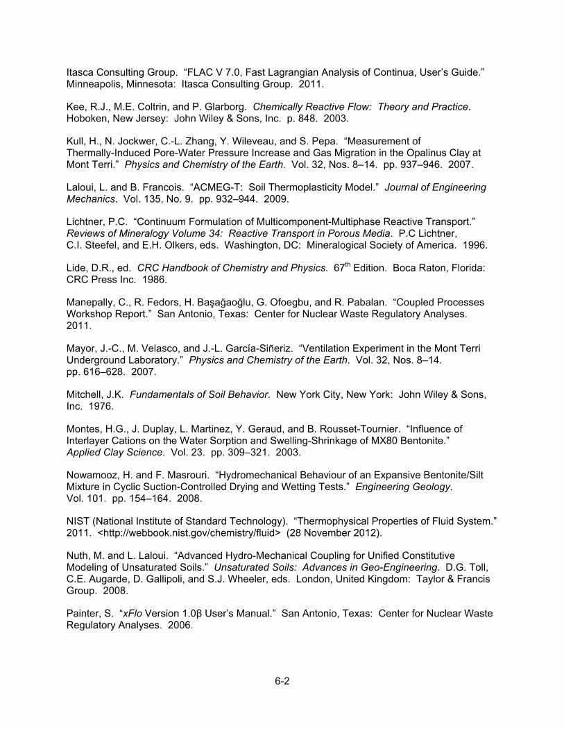
6-2

Itasca Consulting Group. “FLAC V 7.0, Fast Lagrangian Analysis of Continua, User’s Guide.” Minneapolis, Minnesota: Itasca Consulting Group. 2011.

Kee, R.J., M.E. Coltrin, and P. Glarborg. Chemically Reactive Flow: Theory and Practice. Hoboken, New Jersey: John Wiley & Sons, Inc. p. 848. 2003.

Kull, H., N. Jockwer, C.-L. Zhang, Y. Wileveau, and S. Pepa. “Measurement of Thermally-Induced Pore-Water Pressure Increase and Gas Migration in the Opalinus Clay at Mont Terri.” Physics and Chemistry of the Earth. Vol. 32, Nos. 8–14. pp. 937–946. 2007.

Laloui, L. and B. Francois. “ACMEG-T: Soil Thermoplasticity Model.” Journal of Engineering Mechanics. Vol. 135, No. 9. pp. 932–944. 2009.

Lichtner, P.C. “Continuum Formulation of Multicomponent-Multiphase Reactive Transport.” Reviews of Mineralogy Volume 34: Reactive Transport in Porous Media. P.C Lichtner, C.I. Steefel, and E.H. Olkers, eds. Washington, DC: Mineralogical Society of America. 1996.

Lide, D.R., ed. CRC Handbook of Chemistry and Physics. 67th Edition. Boca Raton, Florida: CRC Press Inc. 1986.

Manepally, C., R. Fedors, H. Başağaoğlu, G. Ofoegbu, and R. Pabalan. “Coupled Processes Workshop Report.” San Antonio, Texas: Center for Nuclear Waste Regulatory Analyses. 2011.

Mayor, J.-C., M. Velasco, and J.-L. García-Siñeriz. “Ventilation Experiment in the Mont Terri Underground Laboratory.” Physics and Chemistry of the Earth. Vol. 32, Nos. 8–14. pp. 616–628. 2007.

Mitchell, J.K. Fundamentals of Soil Behavior. New York City, New York: John Wiley & Sons, Inc. 1976.

Montes, H.G., J. Duplay, L. Martinez, Y. Geraud, and B. Rousset-Tournier. “Influence of Interlayer Cations on the Water Sorption and Swelling-Shrinkage of MX80 Bentonite.” Applied Clay Science. Vol. 23. pp. 309–321. 2003.

Nowamooz, H. and F. Masrouri. “Hydromechanical Behaviour of an Expansive Bentonite/Silt Mixture in Cyclic Suction-Controlled Drying and Wetting Tests.” Engineering Geology. Vol. 101. pp. 154–164. 2008.

NIST (National Institute of Standard Technology). “Thermophysical Properties of Fluid System.” 2011. <http://webbook.nist.gov/chemistry/fluid> (28 November 2012).

Nuth, M. and L. Laloui. “Advanced Hydro-Mechanical Coupling for Unified Constitutive Modeling of Unsaturated Soils.” Unsaturated Soils: Advances in Geo-Engineering. D.G. Toll, C.E. Augarde, D. Gallipoli, and S.J. Wheeler, eds. London, United Kingdom: Taylor & Francis Group. 2008.

Painter, S. “xFlo Version 1.0β User’s Manual.” San Antonio, Texas: Center for Nuclear Waste Regulatory Analyses. 2006.

6-3

Painter, S. and M. Seth. “MULTIFO User’s Manual: Two-Phase Nonisothermal Coupled Thermal-Hydrological-Chemical Flow Simulator.” Version 2.0. San Antonio, Texas: Center for Nuclear Waste Regulatory Analyses. 2003.

Pereira, J.M. and E.E. Alonso. “Insights Into the Links Between Microstructure and Bishop’s Parameter for Unsaturated Soils.” 4th Asia-Pacific Conference on Unsaturated Soils. Newcastle, Australia: Australian Geomechanics Society. 2009.

Pruess, K. “TOUGH2—A General Purpose Numerical Simulator For Multiphase Fluid And Heat Flow.” LBL–29400. Berkeley, California: Lawrence Berkeley National Laboratory. 1991.

Rutqvist, J., Y. Ijiri, and H. Yamamoto. “Implementation of the Barcelona Basic Model in TOUGH-FLAC for Simulations of the Geomechanical Behavior of Unsaturated Soils.” Computers & Geosciences. Vol. 37. pp. 751–762. 2011.

Rutqvist, J., Y.-S. Wu, C.-F. Tsang, and G. Bodvarsson. “A Modeling Approach for Analysis of Coupled Multiphase Flow, Heat Transfer, and Deformation in Fractured Porous Rock.” International Journal of Rock Mechanics & Mining Sciences. Vol. 39. pp. 43–442. 2002.

van Genuchten, M.T. “A Closed-Form Equation for Predicting the Hydraulic Conductivity of Unsaturated Soils.” Soil Science Society of America Journal. Vol. 44. pp. 892–898. 1980. Villar, M.V. and A. Lloret. “Influence of Temperature on the Hydro-Mechanical Behavior of a Compacted Bentonite.” Applied Clay Science. Vol. 26. pp. 337–350. 2004.

Wileveau, Y. “THM Behaviour of Host Rock (HE-D) Experiment: Progress Report.” Part 1. TR 2005-03. Wabern, Switzerland: Mont Terri Project. 2005.

Wileveau, Y. and T. Rothfuchs. “THM Behaviour of Host Rock (HE-D) Experiment: Study of Thermal Effects on Opalinus Clay.” TR 2006-01. Wabern, Switzerland: Mont Terri Project. 2007.

APPENDIX A NRC-CNWRA COUPLED PROCESSES WORKSHOP AGENDA

A–1

APPENDIX A

NRC-CNWRA Coupled Processes Workshop

June 27, 2012 9:30am to 4:00 pm EDT

Location: EBB-2C19 at NRC; A237 at CNWRA (Videocon–link)

9:30 Introduction and overview

9:40 DECOVALEX-2015 Task(s) Descriptions

10:40 Development of the Constitutive Model and Implementation in FLAC

11:50 Lunch

1:15 Coupling xFlo-FLAC

2:15 Break

2:30 Modeling Plan Discussions

3:00 Discussions and Summary

4:00 Close-out

APPENDIX B DECOVALEX D-2015 DETAILS

B–1

Table B–1. Tasks List for D-2015

B–2

Table B–2. Participants Details for D-2015

Funding Organizations Country Task(s)

Federal Institute for Geosciences and Natural Resources (BGR) and UFZ

Germany B1

Chinese Academy of Sciences (CAS) China B1, B2, C1

Department of Energy (DOE) USA B1, B2, C2

Federal Nuclear Safety Inspectorate (ENSI) Switzerland B1

Institute of Radiological Protection and Nuclear Safety (IRSN) France A

Japan Atomic Energy Agency (JAEA) Japan B1, B2

Korean Atomic Energy Research Institute (KAERI) Korea B1, B2

Nuclear Decommissioning Authority (NDA) United Kingdom

A, C1

Nuclear Regulatory Commission (NRC) USA B1, A, C1

Radioactive Waste Repository Authority (RAWRA) Czech Republic

A, C1, C2

APPENDIX C xFlo-FLAC Parameters

C–1

Table C–1. Selected Parameter List for xFlo-FLAC Code

Parameters

Thermohydrological Model (xFlo) Symbol

(Units) Sections 3 And 4

Geomechanical Model (FLAC)

Symbols (Units) Section 2 Comments

Absolute (Intrinsic) permeability* K [m2] — Porosity [-] — time-variant In xFlo Void ratio — Void Specific volume — Thermal conductivity of dry rock kdry [W/m-K] — Thermal conductivity of wet rock kwet [W/m-K] — Diffusion coefficient of air in the liquid phase [m2/s] — Specific heat (thermal capacity) Cp [J/K·kg] — — Rock density [kg/m3] — Capillary pressure/matric suction cap[kPa] s [kPa] Both xFlo and FLAC are

implemented in such a way that both Pcap and s are in the positive

realm Soil-moisture characteristic curve Van Genuchten

parameters —

Preconsolidation pressure — Pc (kPa) Slope of normal compression line — Slope of recompression line — Value of specific volume (or void ratio) at a reference pressure smaller than the preconsolidation pressure

— —

Values of the above 4 parameters at different suction values

— —

Coefficient of thermal expansion — —

C–2

Table C–1. Selected Parameter List for xFlo-FLAC Code (continued)

Parameters

Thermohydrological Model (xFlo) Symbol

(Units) Sections 3 and 4

Geomechanical Model (FLAC)

Symbols (Units) Section 2 Comments

Gas and liquid gas phase pressures Pg [Pa], Pl [Pa] ua [Pa], uw [Pa] Phase-dependent (three) state variables: gas saturation; gas pressure; temp (two-phase) air partial pressure; gas pressure; temp (all-gas) mole fraction of air, liquid pressure; temp (all-gas)

Sg [-], Pg [Pa], T[°C]

Pa [Pa], Pg [Pa], T[°C] Xa [Pa], Pl [Pa], T[°C]

— two-phase, all-gas, or no-gas

Type; Infiltration or Dirichlet for Dirichlet gas saturation; gas pressure; temp (two-phase) air partial pressure; gas pressure; temp (all-gas) mole fraction of air; liquid pressure; temp (all-gas)For Infiltration Dissolved air flux; air + water flux; energy flux

Sg [-], Pg [Pa], T[°C] Pa [Pa], Pg [Pa], T[°C] Xa [Pa], Pl [Pa], T[°C] Qa [Mol/m2-Yr]; Qa + w

[Mol/m2-Yr]; Qe [mJ/m2-Yr]

— —

Location(depth) and temporal variations in sourcesource rate for air source rate for total mass (air +water) source rate for energy

Qa [Mol/Yr] Qaw [Mol/Yr] Qe [mJj/Yr]

— —

APPENDIX D EXAMPLE xFlo SIMULATION RESULTS

D–1

In Figures D–5 through D–8, vertical axes are used only for one of the variables listed on the axis title based on the phase state of the problem. For example, if a flow cell exhibits a two-phase condition (e.g., at the 200th element in Figure D–5, the phase variable takes a value of zero (corresponding to a two-phase condition) in the upper left figure, and hence, the vertical axis of the upper right figure is read only for Sg (Table 3-1), and the vertical axis of the lower left figure is read only for Pg (Table 3-1). On the other hand, phase variables for flow cells closer to the top boundary (e.g., 10th element in Figure D–5) take a value of 1, corresponding to an all-gas condition. Therefore, the vertical axis of the upper right figure is read only for Pa (Table 3-1), and the vertical axis of the lower left figure is read only for Pg (Table 3-1).

D–2

Figure D–1. Air (Dissolved) Mass, Total Air and Water Mass, and Energy Content at t = 50 Years, Just Before Initial Porosity of 0.2 Was Elevated to 0.4. Red and blue symbols correspond to constant and variable porosity cases, respectively

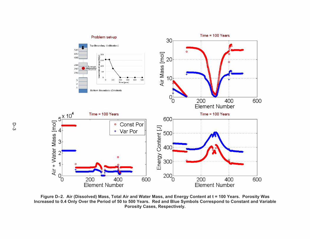
D–3

Figure D–2. Air (Dissolved) Mass, Total Air and Water Mass, and Energy Content at t = 100 Years. Porosity Was Increased to 0.4 Only Over the Period of 50 to 500 Years. Red and Blue Symbols Correspond to Constant and Variable

Porosity Cases, Respectively.

D–4

Figure D-3. Air (Dissolved) Mass, Total Air and Water Mass, and Energy Content at t = 500 Years. Porosity Was Increased to 0.4 Only Over the Period of 50 to 500 Years. Red and Blue Symbols Correspond to Constant and Variable Porosity

Cases, Respectively.

D–5

Figure D–4. Air (Dissolved) Mass, Total Air and Water Mass, and Energy Content at t = 1,000 Years. Porosity Was Increased to 0.4 Only Over the Period of 50 to 500 Years. Red and Blue Symbols Correspond to Constant and Variable

Cases, Respectively.

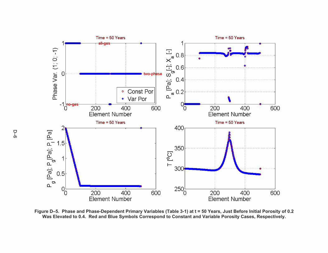
D–6

Figure D–5. Phase and Phase-Dependent Primary Variables (Table 3-1) at t = 50 Years, Just Before Initial Porosity of 0.2 Was Elevated to 0.4. Red and Blue Symbols Correspond to Constant and Variable Porosity Cases, Respectively.

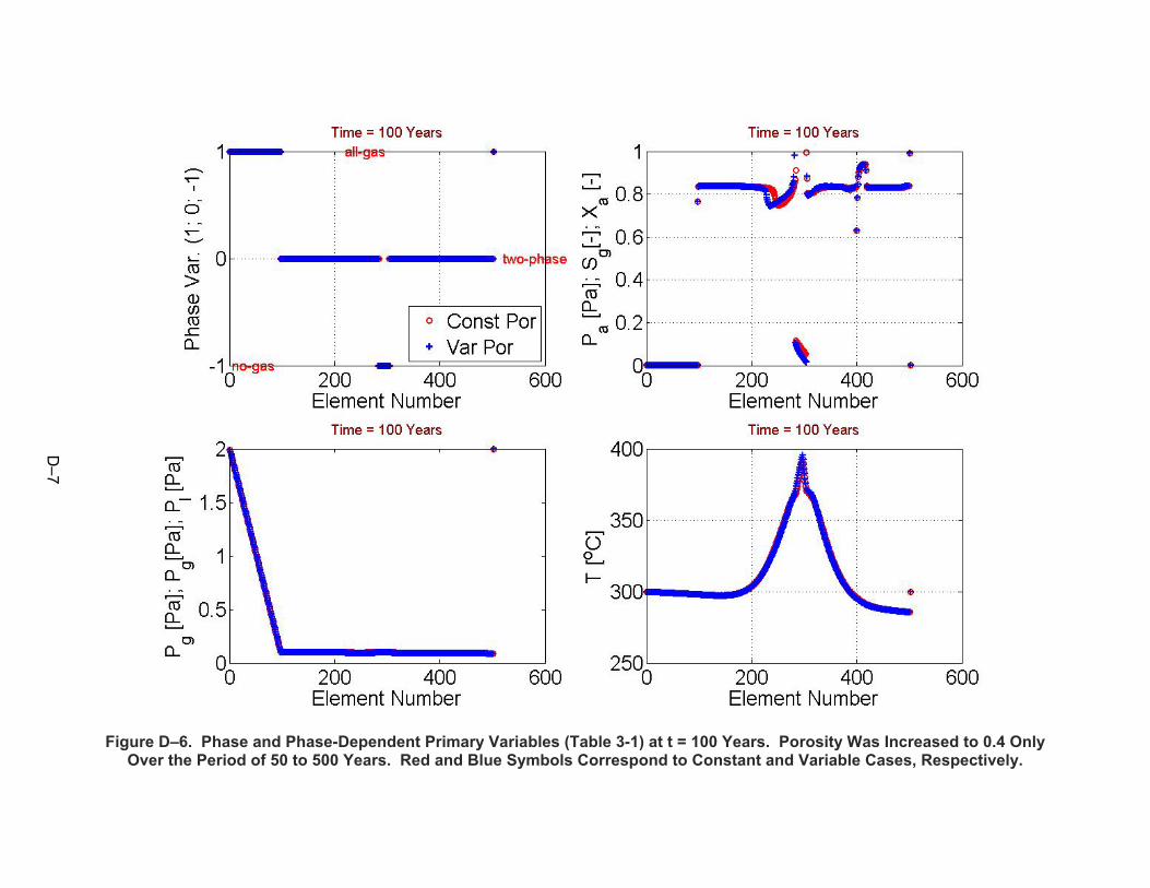
D–7

Figure D–6. Phase and Phase-Dependent Primary Variables (Table 3-1) at t = 100 Years. Porosity Was Increased to 0.4 Only Over the Period of 50 to 500 Years. Red and Blue Symbols Correspond to Constant and Variable Cases, Respectively.

D–8

Figure D–7. Phase and Phase-Dependent Primary Variables (Table 3-1) at t = 500 Years. Porosity Was Increased to 0.4 Only Over the Period of 50 to 500 Years. Red and Blue Symbols Correspond to Constant and Variable Porosity

Cases, respectively.

D–9

Figure D–8. Phase and Phase-Dependent Primary Variables (Table 3-1) at t = 1,000 Years. Porosity Was Increased to 0.4 Only Over the Period of 50 to 500 Years. Red and Blue Symbols Correspond to Constant and Variable Porosity

Cases, Respectively.

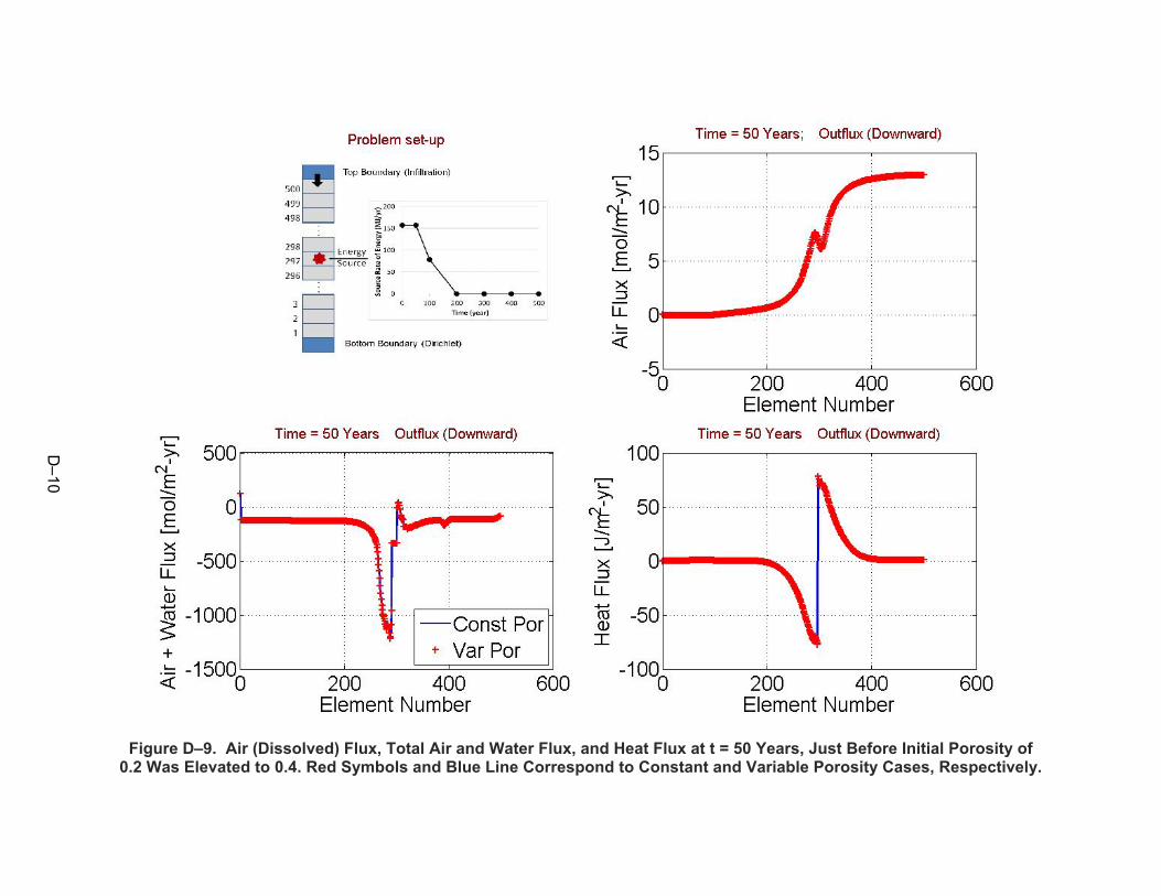
D–10

Figure D–9. Air (Dissolved) Flux, Total Air and Water Flux, and Heat Flux at t = 50 Years, Just Before Initial Porosity of 0.2 Was Elevated to 0.4. Red Symbols and Blue Line Correspond to Constant and Variable Porosity Cases, Respectively.

D–11

Figure D–10. Air (Dissolved) Flux, Total Air and Water Flux, and Heat Flux at t = 100 Years. Porosity Was Increased to 0.4 Only Over the Period of 50 to 500 Years. Red Symbols and Blue Line Correspond to Constant and Variable Porosity

Cases, Respectively.

D–12

Figure D–11. Air (Dissolved) Flux, Total Air and Water Flux, and Heat Flux at t = 500 Years. Porosity Was Increased to 0.4 Only Over the Period of 50 to 500 Years. Red Symbols and Blue Line Correspond to Constant and Variable Porosity

Cases, Respectively.

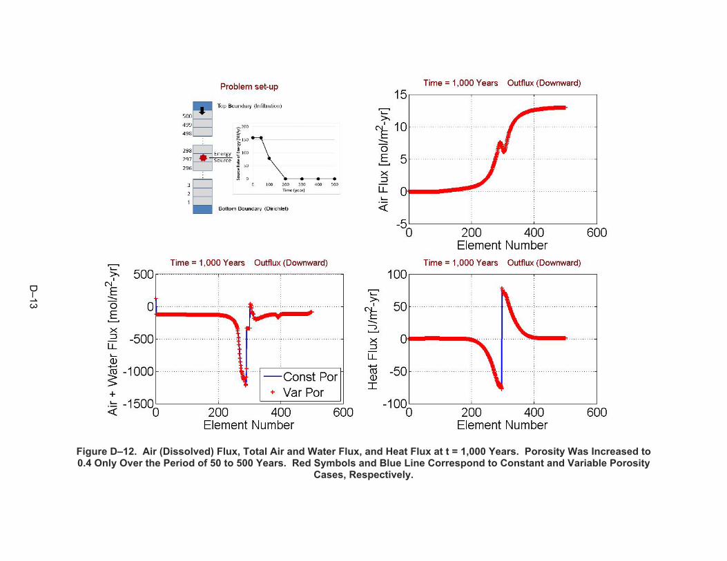
D–13

Figure D–12. Air (Dissolved) Flux, Total Air and Water Flux, and Heat Flux at t = 1,000 Years. Porosity Was Increased to 0.4 Only Over the Period of 50 to 500 Years. Red Symbols and Blue Line Correspond to Constant and Variable Porosity

Cases, Respectively.