Embed Size (px)
Citation preview

Interacting bosons and fermions inone-dimensional lattice potentials
Dissertation
Alexander Mering
Vom Fachbereich Physik der Technischen Universitat Kaiserslautern zur Verleihungdes akademischen Grades
”Doktor der Naturwissenschaften“ genehmigte Dissertation
Betreuer: Prof. Dr. Michael Fleischhauer
Zweitgutachter: Prof. Dr. Sebastian Eggert
Datum der wissenschaftlichen Aussprache: 09. Juni 2010
D 386


Fur Marena


Contents
Abstract i
Zusammenfassung iii
Introduction and foundations 1
Introduction 3
Outline 7
1 Foundations 11
1.1 Bosons in optical lattices . . . . . . . . . . . . . . . . . . . . . 11
1.2 Wannier functions . . . . . . . . . . . . . . . . . . . . . . . . . 19
1.3 Bose-Fermi-Hubbard model . . . . . . . . . . . . . . . . . . . 22
I BFHM in the ultraheavy fermion limit 25
2 Introduction 27
3 Incompressible phases 29
3.1 Ultradeep lattices . . . . . . . . . . . . . . . . . . . . . . . . . 29
3.2 Minimum energy distribution of fermions for small JB . . . . . 32
3.3 Incompressible phases for finite JB . . . . . . . . . . . . . . . 36
3.4 Finite fermion mobility and infinite size scaling . . . . . . . . 43
4 Compressible and partially compressible phases 45
5 Conclusion and outlook 53

CONTENTS
II Fast-fermion induced interactions in the BFHM 55
6 Introduction 57
7 Friedel oscillations: fermion induced superpotential 59
8 Adiabatic elimination of the fermions 65
9 Couplings gd(%F ) for free fermions nj ≡ 0 69
9.1 Calculation of the couplings . . . . . . . . . . . . . . . . . . . 69
9.2 Couplings in real space . . . . . . . . . . . . . . . . . . . . . . 72
9.3 Couplings in momentum space . . . . . . . . . . . . . . . . . . 77
10 Fermionic renormalization and effective Hamiltonian 81
10.1 General framework and initial definitions . . . . . . . . . . . . 82
10.2 Solution of the Dyson equations . . . . . . . . . . . . . . . . . 84
10.3 Green’s function in real space . . . . . . . . . . . . . . . . . . 85
10.4 Expectators and density-density correlator . . . . . . . . . . . 87
10.5 Discussion of the renormalized couplings . . . . . . . . . . . . 91
10.6 The renormalized Hamiltonian . . . . . . . . . . . . . . . . . . 94
11 Self-consistent determination of ηB 97
11.1 Coherent state . . . . . . . . . . . . . . . . . . . . . . . . . . . 97
11.2 Matrix product state . . . . . . . . . . . . . . . . . . . . . . . 99
12 Phase diagram of the effective bosonic model 103
12.1 Zero-hopping phase diagram . . . . . . . . . . . . . . . . . . . 104
12.2 2nd order strong-coupling theory . . . . . . . . . . . . . . . . 109
12.3 Boundary effects with long-range interactions . . . . . . . . . 114
13 Conclusion and outlook 119
III BFHM with nonlinear and band corrections 121
14 Introduction 123
15 Derivation of the multi-band BFHM 125
15.1 Contributing hopping matrix elements . . . . . . . . . . . . . 127
15.2 Contributing interaction matrix elements . . . . . . . . . . . . 127
15.3 Full (relevant) multi-band BFHM . . . . . . . . . . . . . . . . 132
CONTENTS
16 Adiabatic elimination of higher bands 135
16.1 Adiabatic elimination and effective single-band Hamiltonian . 135
16.2 Nonlinear corrections for the first band . . . . . . . . . . . . . 137
16.3 Full (effective) single-band BFHM . . . . . . . . . . . . . . . . 139
17 Real (experimental) parameters 143
17.1 Optical lattice effects . . . . . . . . . . . . . . . . . . . . . . . 143
17.2 Dimensional effects . . . . . . . . . . . . . . . . . . . . . . . . 146
17.3 Bose-Hubbard phase transition . . . . . . . . . . . . . . . . . 148
18 Evaluation of the extensions to the Bose-Hubbard model 151
18.1 One-dimensional lattice . . . . . . . . . . . . . . . . . . . . . . 153
18.2 Three-dimensional lattice . . . . . . . . . . . . . . . . . . . . . 156
19 Conclusion and outlook 161
IV Jaynes-Cummings-Hubbard model 163
20 Introduction 165
21 Lattice bosons coupled to spins 167
21.1 Jaynes-Cummings and Jaynes-Cummings-Hubbard model . . . 167
21.2 Infinite size model for ion chains . . . . . . . . . . . . . . . . . 170
22 Approximative calculation of the phase diagram 173
22.1 Fermion approximation . . . . . . . . . . . . . . . . . . . . . . 173
22.2 Strong-coupling . . . . . . . . . . . . . . . . . . . . . . . . . . 176
22.3 Mean-field theory . . . . . . . . . . . . . . . . . . . . . . . . . 179
23 Benchmarking against nn-JCHM 181
23.1 Strong-coupling results . . . . . . . . . . . . . . . . . . . . . . 181
23.2 Fermion approximation . . . . . . . . . . . . . . . . . . . . . . 182
24 Application to the ion-chain setup 185
25 Conclusion and outlook 191
CONTENTS
Appendix 193
A Ultrafast Fermions 195A.1 Fourier transform of the coupling constants . . . . . . . . . . . 195A.2 Fourier transform of the Green’s functions . . . . . . . . . . . 196A.3 Zero-hopping energies for the phase diagram . . . . . . . . . . 197A.4 Spinless fermions in an alternating potential . . . . . . . . . . 200
B Multi-band physics 207B.1 Calculation of the second order cumulant . . . . . . . . . . . . 207B.2 Bosonic and fermionic correlators . . . . . . . . . . . . . . . . 209B.3 Time integration of the correlators . . . . . . . . . . . . . . . 210B.4 Definition of the constants . . . . . . . . . . . . . . . . . . . . 211
C Jaynes-Cummings-Hubbard model 213C.1 Degenerate perturbation theory . . . . . . . . . . . . . . . . . 213
List of figures 219
Bibliography 223
Publikationen 249
Lebenslauf 251
Danksagung 253


Abstract
Ultracold atoms in optical lattices allow for a fascinating insight in theworld of quantum many-body systems. The comparatively easy control ofmany parameters of these systems gives the opportunity to study manymodels of solid-state theory experimentally without disturbing influences. Inparticular, mixtures of several kinds of atoms promise an insight into physi-cal processes whose observations in solid state systems are close to impossible.
This thesis deals with analytic as well as numeric studies of the ground stateof mixtures of a bosonic and (spin-polarized) fermionic species in periodicpotentials. Experimental realizations of such mixtures in the frameworkof quantum optics already showed several new effects. Furthermore mix-tures are of particular interest since the underlying models have a closerelationship to the research on high-temperature superconductors. Toinvestigate the phase diagram of such mixtures, a treatment in terms of theBose-Fermi-Hubbard model is applied, which is valid for small temperatures.As a result of the large number of free parameters in this system, a detailedinvestigation and comprehensive understanding of the phase diagram willnot cover the full parameter space; restrictions to special cases neverthelessallow for a rather accurate description of physics of this system.
After introducing the model and the basic physics, the first part of thethesis which is based on an earlier diploma thesis deals with the influenceof ultraheavy fermions onto the bosonic phase diagram. At this pointit has to be distinguished, whether the ground state is reached for thefull system or the bosonic sector for a given fermion distribution. In thefirst case, the fermions either arrange themselves with a maximal distancebetween each other or group close to each other. This depends on theeffective coupling between the fermions and is primarily determined by theboson-fermion interaction. The second case describes a bosonic system withbinary disorder, where the special sort of disorder leads, as in the first case,
i

ii ABSTRACT
to the formation of new incompressible phases at non-integer filling. In bothcases, analytic theories are presented, allowing to predict the bosonic phasediagram.
In the second part, the situation of light fermions is considered. The stronglyenhanced fermionic mobility leads to an effective long-range interactionbetween the bosons. A deeper investigation of this interaction shows, thatthe assumption of completely uncoupled fermions leads to divergences whichhave to be renormalized by inclusion of the back-action of the bosons ontothe fermions. Apart from the derivation of the effective bosonic interaction,the resulting bosonic phase diagram is discussed. Starting from the effectivebosonic Hamiltonian it is shown, that the induced interaction leads tothe formation of bosonic density waves, accompanied by fermionic ones,representing a further incompressible phase beside the Mott insulators. Fromthe discussion of boundary effects the existence of a thermodynamicallyinstable phase is found, which comprises density waves and Mott insulatorssimultaneously.
Recent experimental results suggest that the theory of ultracold atoms inoptical lattices based on a first-band model does not explain all occurringeffects. The third part of this thesis is devoted to an effective theory for thefirst band, which takes effects of all higher bands into account by means ofvirtual transitions between the first band and the higher ones. Based onthis effective (renormalized) first-band model, the influence of the higherbands, as well as the influence of the fermions on the bosonic superfluidto Mott-insulator transition is studied and the results are compared toexperimental results.
Finally, part four of this thesis studies the Jaynes-Cummings-Hubbard model,which describes the coupling of two-level atoms in a lattice to a bosonic field.Although this does not describe a boson-fermion mixture, an approach wherethe two-level atoms are treated approximately as fermions allows the easycalculation of the phase diagram. This solution is applied to the case of ionsin a linear Paul trap which present a realization of the Jaynes-Cummings-Hubbard model. Additionally, the findings are compared to results from adegenerate perturbation theory as well as to numerical data.

Zusammenfassung
Ultrakalte Atome in optischen Gittern erlauben einen faszinierenden unddaruber hinaus kontrollierbaren Einblick in die Welt der quantenmechani-schen Vielteilchenphysik. Durch die vergleichsweise einfache Kontrolle vielerParameter dieser Systeme lassen sich eine Vielzahl festkorpertheoretischerModellsysteme ohne storende Einflusse experimentell untersuchen. Soversprechen insbesondere Mischungen mehrerer Atomsorten ein detailliertesStudium physikalischer Prozesse, deren Beobachtung im Festkorper indiesem Maße nicht moglich ist.
In der hier vorliegenden Arbeit werden sowohl analytische, als auchnumerische Untersuchungen an Mischungen einer bosonischen und einer(spin-polarisierten) fermionischen Spezies in einem periodischen Potential imGrundzustand durchgefuhrt. Experimentelle Realisierungen solcher Mischun-gen haben im Rahmen der Quantenoptik bereits eine Vielzahl neuer Effektehervorgebracht. Sie sind weiterhin von besonderem Interesse, da die zugrun-de liegenden Modelle beispielsweise eine direkte Verbindung zur Theorie derHochtemperatur-Supraleitung haben. Fur die hier gemachten Untersuchun-gen des Phasendiagramms wird das Bose-Fermi-Hubbard-Modell verwendet,welches solche Mischungen im Fall niedriger Temperaturen beschreibt.Durch die Vielzahl freier Parameter in diesem System kann eine detaillierteUntersuchung und ein genaues Verstandnis des Phasendiagramms nursehr schlecht den gesamten Parameterraum abdecken; Beschrankungen aufspezielle Parameterbereiche erlauben hier dennoch einen fundierten Einblick.
Nach einer Einfuhrung in das Modell und die dadurch beschriebene Physikwird im ersten Teil dieser Arbeit aufbauend auf meiner vorangegangenenDiplomarbeit der Einfluß sehr schwerer Fermionen auf das bosonischePhasendiagramm studiert. Hier ist zu unterscheiden, ob das Gesamtsystemoder nur der bosonische Sektor bei fest vorgegebener Fermionenverteilungden Grundzustand erreicht. Im ersten Fall ergibt sich ein Bild, in dem
iii

iv ZUSAMMENFASSUNG
die Fermionen entweder einen maximalen Abstand zueinander bevorzugenoder sich in benachbarten Gitterplatzen ansammeln. Dies hangt von einereffektiven Kopplung der Fermionen untereinander ab und ist primar durchdie Boson-Fermion-Wechselwirkung bestimmt. Der zweite Fall beschreibtein bosonisches System mit einer binaren Unordnung, wobei die spezielleUnordnung ebenso wie im ersten Fall zur Ausbildung neuer inkompressiblerPhasen mit nicht-ganzzahliger Fullung fuhrt. Fur beide Falle werdenanalytische Theorien prasentiert, die eine Vorhersage fur das bosonischePhasendiagramm erlauben.
Der zweite Teil betrachtet die Situation sehr leichter Fermionen. Hier fuhrtdie, im Vergleich zu den Bosonen stark erhohte Mobilitat der Fermionenzu einer durch diese induzierten effektiven Wechselwirkung zwischen denBosonen. Eine genaue Untersuchung dieser Wechselwirkung zeigt, dasseine Annahme vollig entkoppelter Fermionen Divergenzen liefert, welchejedoch durch eine Berucksichtigung der Ruckwirkung der Bosonen aufdie Fermionen renormalisiert werden konnen. Neben der Herleitung dereffektiven bosonischen Wechselwirkung steht die Diskussion des bosonischenPhasendiagramms im Vordergrund. Ausgehend vom effektiven bosonischenHamilton-Operator lasst sich zeigen, dass die induzierte Wechselwirkungdurch die Fermionen zur Ausbildung von bosonischen und damit auchfermionischen Dichtewellen fuhrt, welche eine weitere inkompressible Phaseneben den bekannten Mott-Isolatoren beschreibt. Eine Diskussion desEinflusses der Randbedingungen zeigt uberdies noch die Existenz von ther-modynamisch instabilen Phasen in denen Dichtewellen und Mott-Isolatorenkoexistieren.
Aktuelle experimentelle Ergebnisse zeigen, dass eine Beschreibung ultrakal-ter Atome in optischen Gittern im Rahmen eines Einband-Modells nicht alleEffekte beschreiben kann. Dazu wird im dritten Teil eine effektive Theoriedes ersten Bandes entwickelt, welche den Einfluss aller hoheren Banderdurch virtuelle Ubergange zwischen dem ersten und den hoheren Bandernberucksichtigt. Im Rahmen dieses effektiven (renormierten) Einband-Modellswird der Einfluss der hoheren Bander sowie der Fermionen auf den bosoni-schen Superfluid-zu-Mott-Isolator Ubergang untersucht und in Relation zuexperimentellen Ergebnissen gesetzt.
Abschließend wird in Teil vier das Jaynes-Cummings-Hubbard-Modell be-trachtet. Dieses beschreibt die Kopplung von Zwei-Niveau-Atomen in einemregelmaßigen Gitter an ein bosonisches Feld. Obwohl hier zwar keine Mi-schung aus Bosonen und Fermionen vorliegt, erlaubt die Naherung die Zwei-

ZUSAMMENFASSUNG v
Niveau-Atome als Fermionen zu betrachten (effektives Fermionenmodell) eineeinfache Bestimmung des Phasendiagramms dieses Modells. Die so gefundeneLosung wird dann zur Beschreibung von Ionen in einer linearen Paul-Falleangewendet, was eine Realisierung des Jaynes-Cummings-Hubbard-Modellsdarstellt. Die Ergebnisse dieser Naherung werden schließlich zu einer entar-teten Storungstheorie sowie numerischen Resultaten in Beziehung gesetzt.


Introduction and foundations
1


Introduction
Starting from the development of efficient laser cooling techniques for neutralatoms [1, 2, 3], the field of ultracold atoms developed quickly, reaching thelong-term goal of a Bose-Einstein condensate (BEC) [4, 5] in Sodium [6, 7],Rubidium [8, 9] and Lithium [10] in the mid 1990th. More elaborate coolingsteps finally led to the achievement of a degenerate Fermi gas [11, 12] andfurther improvements in the experiments subsequently allowed to imposeoptical lattices to the BEC (for an overview see [13]), culminating in thefirst observation of a bosonic superfluid to Mott-insulator transition [14] inRubidium [15]. For the fermionic analog, very recently the Mott insulatingstate for stronger lattices was reached [16, 17].
Apart from realizations in ultracold atoms, BECs can also be observed inother physical systems as for instance in magnons in the solid state [18], exci-ton polaritons in semiconductor microcavities [19] or, with some limitationsin liquid Helium as in the early works of [20, 21]. Even Cooper-pairs [22] insuperconduction theory [23, 24] can be seen as a BEC. However, only withinthe framework of quantum optics it is possible to manipulate importantsystem parameters such as the interaction between the constituents or thegeometry in a precise way. Because of this and the fact that the natureof the resulting ground and excitated states can be studied by a variety ofdifferent experimental methods, ultracold atoms provide the state-of-the-artapproach to study many-body physics experimentally under maximumexternal control.
Alkali elements are most suitable for laser cooling and trapping because oftheir atomic level structure [25], but earth-alkali elements (Calcium [26],Strontium [27]) and other elements as Ytterbium [28], metastable Helium[29, 30] and Hydrogen [31] could also be used for a BEC. Important isthe achievement of a BEC of Chromium [32], since Cr has a large dipolemoment, thus realizing a dipolar BEC with intrinsic long-range (orientationdependent) interactions.
3
4 INTRODUCTION
After the step of a simultaneous trapping of bosonic (e.g. 7Li, 41K or 87Rb)and fermionic isotopes (e.g 6Li or 40K) of the same or different elements[33, 34, 35, 36], the combination of the degenerate mixture with an opticallattice setup [37, 38] opened the route to study a large variety of differentphysical model systems. The most prominent is the Bose-Fermi-Hubbardmodel [39], introduced in section 1.3, which is the key model studied in thisthesis.
Beyond the issues of preparation of the BEC or degenerate mixtures, a largeprogress in the manipulation and analysis of the ultracold-atom systemwas made in the last decade. Starting from simple absorption images ofthe atomic cloud, modern setups allow for a direct, in-situ, imaging of atwo-dimensional BEC [40, 41] or the usage of electron microscopy [42] withsingle-site resolution. Additional to imaging, the physics of the BEC (withour without lattice) was studied by noise interferometry [43] as well as byseveral spectroscopic methods, including microwave [44], lattice modulation[45, 46], radio-frequency [47] or Bragg spectroscopy [48, 49]. The lattermethod was recently extended to a momentum-resolved measurement ofthe excitation spectrum, allowing to study the full band structure as wellas interaction effects on it [50, 51]. For further details of the experimentalmethods refer to the review [13] and references therein. [52] gives ashort introduction on the realization of a BEC using atom chips, anotherpromising implementation of ultracold atoms.
As latest points in the long list of achievements in the systems of ultracoldatoms, the controlled realization of (cold) chemical reactions [53, 54, 55]and the in-deep study of genuine many-body states such as Efimov-trimers[56, 57, 58] shows the enormous possibilities of ultracold atoms. Nevertheless,many questions are still open. Though providing a fully controllable tool forthe simulation of well known Hamiltonians ranging from the Bose-Hubbardmodel [59], the Hubbard model [16, 17] to effective spin models [60, 61, 62] invarious lattice geometries (dimensionality [63, 64], lattice types [65, 66, 67]or including disorder [68, 69, 70, 71]), the nature of the different quantumphase transitions still gives open questions. Considering ultracold atomsas a quantum simulator [72], the implementations of quantum phasegates [73, 74] are a further step towards a (scalable) quantum informationtechnology. As a far goal, the understanding of various important, but yetunclear phenomena such as high-TC superconductivity [75, 76, 77] or thephysics of strongly imbalanced interacting fermions [78, 79] are prominentoutstanding problems to be explored. For all of these kinds of models, ul-
INTRODUCTION 5
tracold atoms provide a controllable environment to study individual effectsof the system which could not be discriminated against further effects inother experimental realizations. Finally, the application of the lattice setupopens the route to single-atom trapping which is important to metrology [80].
Focussing on the physics of mixtures of bosons and fermions in the opticallattice, described by the Bose-Fermi-Hubbard model, we study in this thesisthe influence of the fermionic admixture on the well understood bosonic phasediagram. This model is of special interest due to its relation for instance tothe coupling of fermions to phonons [81], fermionic polarons [82] or compos-ite particles [83]. In a series of experiments [37, 38, 84] a strong influence ofthe fermions to the bosonic superfluid to Mott-insulator transition was seen.Similar experiments in Bose-Bose mixture reveal that only a small overlapof the different atomic clouds suffices to observe the effect of inter-speciesinteractions [85]. Though some analytics and numerics has been done to un-derstand these effects [86, 87, 88, 89, 90], several aspects are not understoodyet. Limiting on different regions of the parameter space, we develop analyticapproaches to provide a better understanding of the physics of interactingbosons and fermions, supported by numerical simulations. This allows forthe construction of the bosonic phase diagram as well as the prediction ofqualitatively new phases.

Outline
Throughout the whole thesis we present different approaches to the physicsof interacting bosons and fermions, each of them allowing for the predictionof the phase diagram in different parameter regimes. Starting with thediscussion of the general physics of ultracold bosons in optical lattices, thefirst part of this thesis deals with the physics of the Bose-Fermi-Hubbardmodel with vanishing fermionic mobility. Extending the results from a priordiploma thesis, we study the influence of the fermions on the bosonic phasediagram. In this limit, the fermions are treated as a source of disorder whichis assumed to be either quenched or annealed. In both cases, incompressiblephases with non-integer fillings arise together with the prediction of aBose-glass phase [Mering2008].
In the second part, the opposite limit is considered. Assuming the fermionsto be ultrafast, i.e., having almost infinite mobility, an effective bosonictheory yielding induced long-range density-density interactions is derived[Mering2010]. A first treatment of the induced interactions reveals the needfor a renormalization scheme, including the back-action of the resultingbosonic charge-density wave phase to the fermions. Within the renor-malized effective model, a strong-coupling theory gives analytic estimatesfor the phase diagram, pointing to the existence of thermodynamicallyunstable phases of coexistence between a charge-density wave phase anda Mott insulator. Here, boundary issues are crucial for the understand-ing of the system, leading to phases displaying a spatial separation of aMott insulator and a charge-density wave, also seen in numerical simulations.
Ultracold atoms in deep optical lattices are usually described by means ofa first-band model. Recent experimental results suggest however, that thisapproach does not hold for a full understanding of certain aspects of thesesystems. This problem, being discussed in the third part of this thesis, isresolved by the inclusion of the higher bands into the Bose-Fermi-Hubbard
7
8 OUTLINE
model. Though contributing to the Hamiltonian, an adiabatic eliminationof these higher bands condenses their effect to an effective first-banddescription extended by contributions due to virtual transitions to thehigher bands. Starting from this effective Hamiltonian, the effect of thehigher bands as well as the effect of the fermions to the bosonic superfluidto Mott-insulator transition is studied and compared to experimental results.
The final part of this thesis studies the Jaynes-Cummings-Hubbard modelwhich describes the physics of two-level atoms coupled to a bosonic latticefield. Approximating the two-level systems as fermions [Mering2009], theJaynes-Cummings-Hubbard model is easily solved with analytic expressionsfor the phase diagram. Special application of this solution to the physicsof ions in a linear Paul trap displaying long-ranged bosonic hopping givesa first estimate for the phase diagram of this system. Perturbation theoryas well as numerical results for the phase diagram finally validate the madeapproximations.


CHAPTER 1
Foundations
In this chapter we provide the basic theory for the description of ultracoldatoms and mixtures in optical lattices and give a short overview over the mostimportant properties of the different phases. Before treating the mixture, wefocus on the discussion of the pure bosonic system, introducing the mainquantities and defining the notation. All this is done for a one-dimensionalsystem.
1.1 Bosons in optical lattices
Jaksch et al. realized in a pioneering work [59], that ultracold bosonic atomsin an optical lattice are well described by the Bose-Hubbard model. Assuminga local interaction V (z−z′) = gBBδ(z−z′) for the bosons with gBB = 4π~2
mBaBB
and aBB being the s-wave scattering length, the continuous Hamiltonianreads
H =
∫dzΨ†B(z)
[− ~2
2mB
∆ + V BPot(z)
]ΨB(z)
+gBB
2
∫dzΨ†B(z)Ψ†B(z)ΨB(z)ΨB(z).
(1.1)
A potential V BPot(z) = ηB sin2(kz) is considered with k being the wave-vector
of the optical lattice laser and ηB the amplitude of the potential. Noadditional harmonic confinement is included. Details about the physicaleffects of the lattice potential can be found in section 17.1 and in [13, 91].Here we shortly summarize the main features of this system.
11

12 CHAPTER 1. FOUNDATIONS
For the field operators it is convenient to switch to a localized basis in termsof Wannier functions (see section 1.2), i.e., decomposing ΨB(z) as
ΨB(z) =∑j
aj wB(z − ja) (1.2)
with a being the lattice spacing. We only incorporated Wannier functionsfrom the first Bloch band, which is a good approximation for deep latticesand low temperatures, i.e., if the temperature is small compared to the bandgap1. The replacement of the field operators in the continuous Hamiltonianleads to a lattice model, the well known Bose-Hubbard model [14]:
HBHM = −JB∑j
(a†j aj+1 + a†j+1aj
)+U
2
∑j
nj (nj − 1) + ∆B
∑j
nj. (1.3)
nj = a†j aj is the number operator and a†j (aj) the bosonic creation (annihi-lation) operator at lattice site j. This model also describes the physics ofliquid 4He in pouros media [92] or an array of Josephson junctions [93, 94].The first term is the kinetic energy, i.e., the hopping of a single particle fromone site to its nearest-neighbors with amplitude
JB = −∫
dz wB(z − a)
[− ~2
2mB
∂2
∂z2+ V B
Pot(z)
]wB(z), (1.4)
the second term the local nonlinearity with
U = gBB
∫dz wB(z)wB(z)wB(z)wB(z) (1.5)
and the last term is the band energy
∆B =
∫dz wB(z)
[− ~2
2mB
∂2
∂z2+ V B
Pot(z)
]wB(z). (1.6)
A discussion of the properties of these amplitudes as a function of the latticedepth ηB is found in the next section. Generally, we set the energy scaleby U = 1. All other amplitudes, though not explicitly written, are referredto this energy. In Hamiltonian (1.3) no other contributions occur beside
1In part III we show that this assumption is too strong and does not allow a fullunderstanding of experimental results; higher bands are important in the experimentalsituation but here they unnecessarily complicate the system and are henceforth left outthroughout the whole thesis besides part III.

1.1. BOSONS IN OPTICAL LATTICES 13
local interactions and nearest-neighbor hopping. This is a common simpli-fication for these kinds of models, since all other amplitudes are much smaller.
For the treatment of the Bose-Hubbard model, the band energy is not im-portant as it gives just an energy shift since the total number of particlesN =
∑j nj commutes with the Hamiltonian. This accounts for the de-
scription of the system in the canonical ensemble, i.e., fixing the number ofparticles. For the discussion of the phase boundaries, this description turnsout to be more suitable than the grand-canonical ensemble, i.e., including achemical potential described by
K = H − µB∑j
nj. (1.7)
Nevertheless the different phases are discussed in the (µB, JB)-plane wherethe chemical potential, which gives the energy cost when changing the num-ber of particles, is defined as
µB =∂E
∂N= E(N + 1)− E(N) (1.8)
This also leads to the definition of the compressibility which accounts for thechange of the number of particles with the chemical potential:
κ =∂〈N〉∂µB
. (1.9)
For phases with non-zero compressibility, the system in ungapped (with re-spect to particle-hole excitations), i.e., it does not cost energy to change thenumber of particles. For the Bose-Hubbard model (1.3), two different phasesexist, distinguished by the compressibility.
a) Plain Bose-Hubbard model
The model described in (1.3) will be referred to as the plain Bose-Hubbardmodel, which is the basis of our discussions. We will present two importantextensions later. First we discuss the phase diagram of the plain model.
In the interaction dominated regime U JB and for commensurate fillingN = nL, the ground state is given by the so-called Mott insulator, displayingthe same number of particles n on each lattice cite, i.e.,
|Ψ〉Mott ∼∑j
(a†j
)n|0〉 . (1.10)
14 CHAPTER 1. FOUNDATIONS
A single particle-hole excitation a†j al 6=j |Ψ〉Mott has an extra energy U (forJB = 0) compared to the Mott insulator and therefore the Mott insulatingphase is incompressible; it costs energy to add or remove a particle.
In the hopping dominated regime U JB and for any filling, the groundstate is a superfluid with
|Ψ〉SF ∼
(∑j
a†j
)N
|0〉 . (1.11)
This state does not display a particle-hole gap, it is compressible.
For vanishing hopping JB = 0, the phase diagram is easily constructed for thegrand-canonical Bose-Hubbard Hamiltonian (1.7). The Hamiltonian becomeslocal and the number n of particles per site which minimizes the energy isgiven by
n = max0, [1/2 + µB], (1.12)
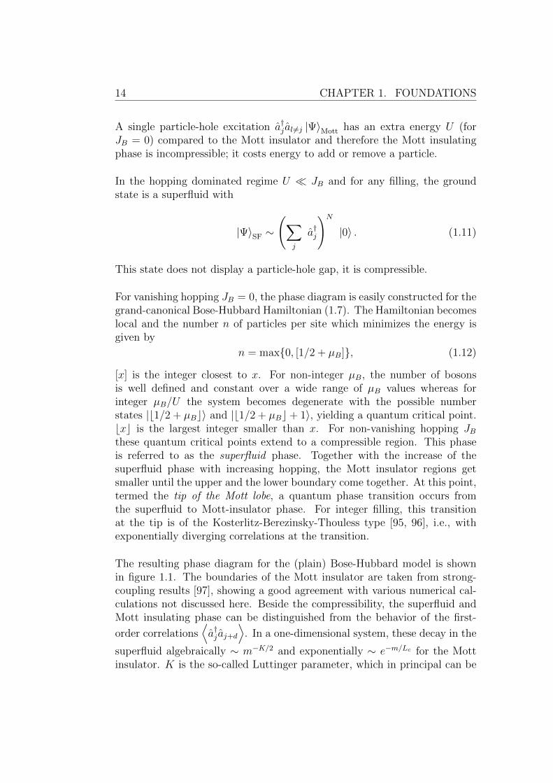
[x] is the integer closest to x. For non-integer µB, the number of bosonsis well defined and constant over a wide range of µB values whereas forinteger µB/U the system becomes degenerate with the possible numberstates |b1/2 + µBc〉 and |b1/2 + µBc+ 1〉, yielding a quantum critical point.bxc is the largest integer smaller than x. For non-vanishing hopping JBthese quantum critical points extend to a compressible region. This phaseis referred to as the superfluid phase. Together with the increase of thesuperfluid phase with increasing hopping, the Mott insulator regions getsmaller until the upper and the lower boundary come together. At this point,termed the tip of the Mott lobe, a quantum phase transition occurs fromthe superfluid to Mott-insulator phase. For integer filling, this transitionat the tip is of the Kosterlitz-Berezinsky-Thouless type [95, 96], i.e., withexponentially diverging correlations at the transition.
The resulting phase diagram for the (plain) Bose-Hubbard model is shownin figure 1.1. The boundaries of the Mott insulator are taken from strong-coupling results [97], showing a good agreement with various numerical cal-culations not discussed here. Beside the compressibility, the superfluid andMott insulating phase can be distinguished from the behavior of the first-
order correlations⟨a†j aj+d
⟩. In a one-dimensional system, these decay in the
superfluid algebraically ∼ m−K/2 and exponentially ∼ e−m/Lc for the Mottinsulator. K is the so-called Luttinger parameter, which in principal can be
1.1. BOSONS IN OPTICAL LATTICES 15
bosonic hopping JB
chem
ical pote
ntial µ
B
0 0.05 0.1 0.15 0.2 0.25 0.3 0.35 0.4
−0.5
0
0.5
1
1.5
2
2.5
3
3.5
4
superfluid
n=4
n=3
n=2
n=1
n=0
Figure 1.1: Phase diagram of the Bose-Hubbard model. Gray regions arethe Mott insulators, outside lies the superfluid region. The phase boundarieswere obtained according to [97]. The interaction energy U = 1 is set asenergy scale. Within the Mott insulators, the first-order correlations decayexponentially, within the superfluid algebraically.
calculated from other approaches as Bethe ansatz [98, 99] and the algebraicdecay is seen from a bosonization approach [99, 100, 101, 102, 103].
b) Disordered Bose-Hubbard model
In the plain Bose-Hubbard model, no locally varying potential is present.Including local potentials as
HdBHM = HBHM +∑j
εjnj, (1.13)
the resulting Bose-Hubbard Hamiltonian allows for a description of variousdifferent situations such as bosons in an external (harmonic) confinementwith εj = ω (j − L/2)2, superlattice structures as εj = V δ(sin(πj/2)) ordisordered systems with εj ∈ [−∆/2,∆/2] chosen randomly.
Here we discuss the situation of a weak (∆ < U), bound random disorder.For strong or unbound disorder the situation qualitatively stays the same,where the main difference to weak disorder is given by the full vanishing ofall Mott insulating lobes. The disorder distribution itself does not play anyrole for the discussion of the phase diagram with one exception pointed out

16 CHAPTER 1. FOUNDATIONS
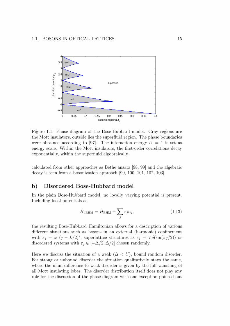
Figure 1.2: Phase diagram of the disordered Bose-Hubbard model in threedimensions for different strengths of the disorder ∆ taken from [71]. Forvanishing disorder, the typical lobe structure is seen with a decrease of theMott lobes (MI) for weak (∆ < U) disorder. For large or unbound disorder,all Mott lobes vanish with only a Bose glass (BG) and superfluid phase (SF)remaining.
in section 3.1.
For zero bosonic hopping (JB = 0) and weak disorder, the disorder leadsto a shift of the upper and lower boundary of the Mott insulators. Due tothe inhomogeneity of the system and the continuous disorder distribution,additional particles can always be added without cost in energy. This holds,until commensurate filling is reached, according to the Mott insulating state.The energy to add another particle is now given by the change in interactionenergy nU as well as the smallest local energy min(εj) = −∆/2, the chemicalpotential for the upper boundary of the Mott insulator therefore equalsnU − ∆/2. Accordingly, the lower boundary is given by (n − 1)U + ∆/2.This indicates a shrinking of the Mott insulating region by ∆ with theappearance of a compressible phase in between2 (see figure 1.2).
The Mott insulating gap closes with increasing hopping as in the plain sys-tem. The intermediate compressible phase turns out to be of a differentcharacter than the superfluid. This is seen in the correlations of the system,which still decay exponentially hence indicating a localization of the bosons,
2This explains the distinction between weak and strong disorder. For the strong dis-order case, the disorder induced shifts of the upper and lower boundaries are beyond thewidth of the Mott insulator.
1.1. BOSONS IN OPTICAL LATTICES 17
as well as in the vanishing superfluid fraction
%S =2L2
π2NB
(Eapbc − Epbc
). (1.14)
The superfluid fraction is defined by the energy difference of the ground statesof the system with anti-periodic and periodic boundary conditions [104, 105],thus accounting for the response of the system to a phase gradient. Thiscompressible, not superfluid Bose-glass phase is a direct consequence of thedisorder and up to now a main research object theoretically and experimen-tally. Again, ultracold atoms allow for the observation of this glass phase incontrolled experiments [69, 71, 106] with a clear observation of the predictedproperties.
c) Bose-Hubbard model with nearest-neighbor inter-actions
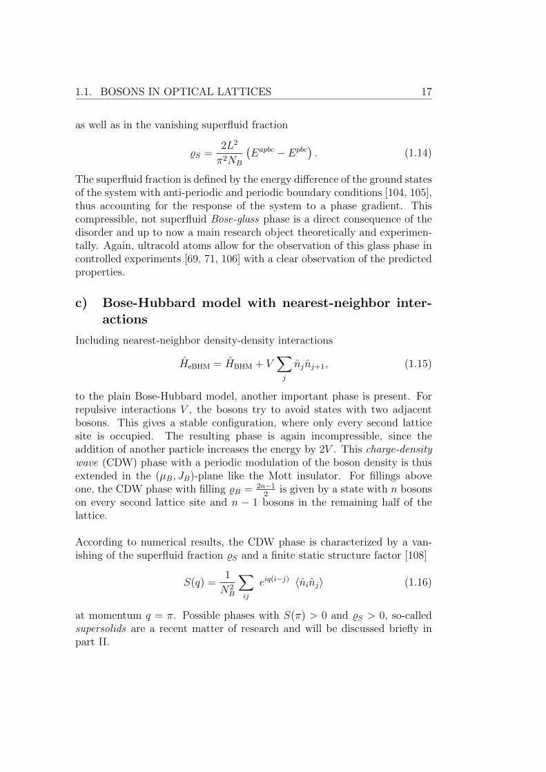
Including nearest-neighbor density-density interactions
HeBHM = HBHM + V∑j
njnj+1, (1.15)
to the plain Bose-Hubbard model, another important phase is present. Forrepulsive interactions V , the bosons try to avoid states with two adjacentbosons. This gives a stable configuration, where only every second latticesite is occupied. The resulting phase is again incompressible, since theaddition of another particle increases the energy by 2V . This charge-densitywave (CDW) phase with a periodic modulation of the boson density is thusextended in the (µB, JB)-plane like the Mott insulator. For fillings aboveone, the CDW phase with filling %B = 2n−1
2is given by a state with n bosons
on every second lattice site and n − 1 bosons in the remaining half of thelattice.
According to numerical results, the CDW phase is characterized by a van-ishing of the superfluid fraction %S and a finite static structure factor [108]
S(q) =1
N2B
∑ij
eiq(i−j) 〈ninj〉 (1.16)
at momentum q = π. Possible phases with S(π) > 0 and %S > 0, so-calledsupersolids are a recent matter of research and will be discussed briefly inpart II.
18 CHAPTER 1. FOUNDATIONS
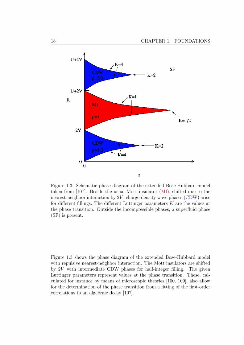
Figure 1.3: Schematic phase diagram of the extended Bose-Hubbard modeltaken from [107]. Beside the usual Mott insulator (MI), shifted due to thenearest-neighbor interaction by 2V , charge-density wave phases (CDW) arisefor different fillings. The different Luttinger parameters K are the values atthe phase transition. Outside the incompressible phases, a superfluid phase(SF) is present.
Figure 1.3 shows the phase diagram of the extended Bose-Hubbard modelwith repulsive nearest-neighbor interaction. The Mott insulators are shiftedby 2V with intermediate CDW phases for half-integer filling. The givenLuttinger parameters represent values at the phase transition. These, cal-culated for instance by means of microscopic theories [100, 109], also allowfor the determination of the phase transition from a fitting of the first-ordercorrelations to an algebraic decay [107].

1.2. WANNIER FUNCTIONS 19
1.2 Wannier functions
In the derivation of the Bose-Hubbard Hamiltonian (1.3), the field operatorswere expanded in the local basis of Wannier functions. Following [110], theseare obtained from the solution of the single particle Schrodinger equation(
− ∂2
∂z2+ ηB sin2(z)
)Φ(z) = E Φ(z), (1.17)
where all energies are given in units of the recoil energy Erec = ~2k22mB
andall lengths in units of 1/k. Since the system is periodic with period π,the Hamiltonian commutes with the (discrete) translation operator and theeigenfunctions are given in terms of Bloch waves [111]
Φn,p(z) = un,p(z)eipz. (1.18)
un,p(z) is periodic with the lattice spacing. The eigenenergies of form certainranges En,p with n giving the different Bloch bands. Dealing with the notionof different sites, the delocalized Bloch waves Φn,p(z) are replaced by themore suitable Wannier functions [112], being localized within the differentpotential minima. They are given by
wn(z) =1√2
1∫−1
dp Φn,p(z), (1.19)
but are not uniquely defined due to an arbitrary phase factor. Neverthelessthey fall off exponentially [113, 114] and can be chosen to be symmetric inthe odd bands and antisymmetric in the even bands [113].
Only in the limit ηB → ∞ the Wannier functions have simple analytic ex-pressions. Here the lattice potential is properly approximated by a harmonicpotential, giving the oscillator eigenfunctions for the Wannier functions inthe harmonic oscillator approximation. Numerically, the Wannier functionsare calculated from the Schrodinger equation (1.17) together with the Blochwaves (1.18). For the periodic part in (1.18), the differential equation((
−i ∂∂z
+ p
)2
+ ηB sin2(z)
)un,p(z) = En,p un,p(z) (1.20)
together with a Fourier transform
un,p(z) =∑m
a(n,p)m e2imz (1.21)
20 CHAPTER 1. FOUNDATIONS
−3 −2 −1 0 1 2 3−1.5
−1
−0.5
0
0.5
1
1.5
2
normalized coordinate z
Wannie
r fu
nction w
b(z
)
first band
second band
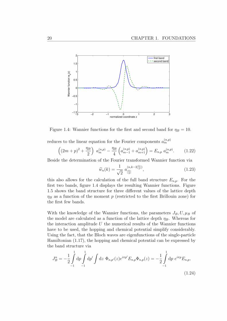
Figure 1.4: Wannier functions for the first and second band for ηB = 10.
reduces to the linear equation for the Fourier components a(n,p)m(
(2m+ p)2 +ηB2
)a(n,p)m − ηB
4
(a
(n,p)m−1 + a
(n,p)m+1
)= En,p a
(n,p)m . (1.22)
Beside the determination of the Fourier transformed Wannier function via
wn(k) =1√2a
(n,k−2[ k2
])
[ k2
], (1.23)
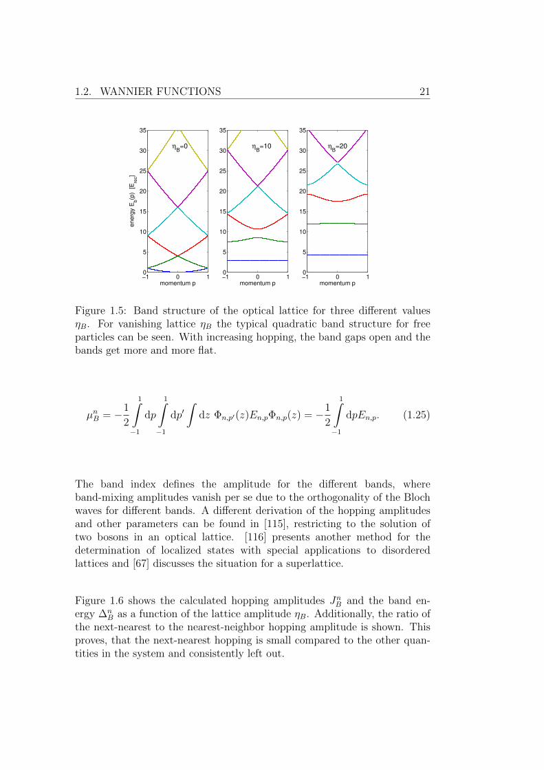
this also allows for the calculation of the full band structure En,p. For thefirst two bands, figure 1.4 displays the resulting Wannier functions. Figure1.5 shows the band structure for three different values of the lattice depthηB as a function of the moment p (restricted to the first Brillouin zone) forthe first few bands.
With the knowledge of the Wannier functions, the parameters JB, U, µB ofthe model are calculated as a function of the lattice depth ηB. Whereas forthe interaction amplitude U the numerical results of the Wannier functionshave to be used, the hopping and chemical potential simplify considerably.Using the fact, that the Bloch waves are eigenfunctions of the single-particleHamiltonian (1.17), the hopping and chemical potential can be expressed bythe band structure via
JnB = −1
2
1∫−1
dp
1∫−1
dp′∫
dz Φn,p′(z)eiπp′En,pΦn,p(z) = −1
2
1∫−1
dp eiπpEn,p,
(1.24)
1.2. WANNIER FUNCTIONS 21
−1 0 10
5
10
15
20
25
30
35
momentum p
energ
y E
b(p
) [E
rec]
−1 0 10
5
10
15
20
25
30
35
momentum p−1 0 10
5
10
15
20
25
30
35
momentum p
ηB=0 η
B=10 η
B=20
Figure 1.5: Band structure of the optical lattice for three different valuesηB. For vanishing lattice ηB the typical quadratic band structure for freeparticles can be seen. With increasing hopping, the band gaps open and thebands get more and more flat.
µnB = −1
2
1∫−1
dp
1∫−1
dp′∫
dz Φn,p′(z)En,pΦn,p(z) = −1
2
1∫−1
dpEn,p. (1.25)
The band index defines the amplitude for the different bands, whereband-mixing amplitudes vanish per se due to the orthogonality of the Blochwaves for different bands. A different derivation of the hopping amplitudesand other parameters can be found in [115], restricting to the solution oftwo bosons in an optical lattice. [116] presents another method for thedetermination of localized states with special applications to disorderedlattices and [67] discusses the situation for a superlattice.
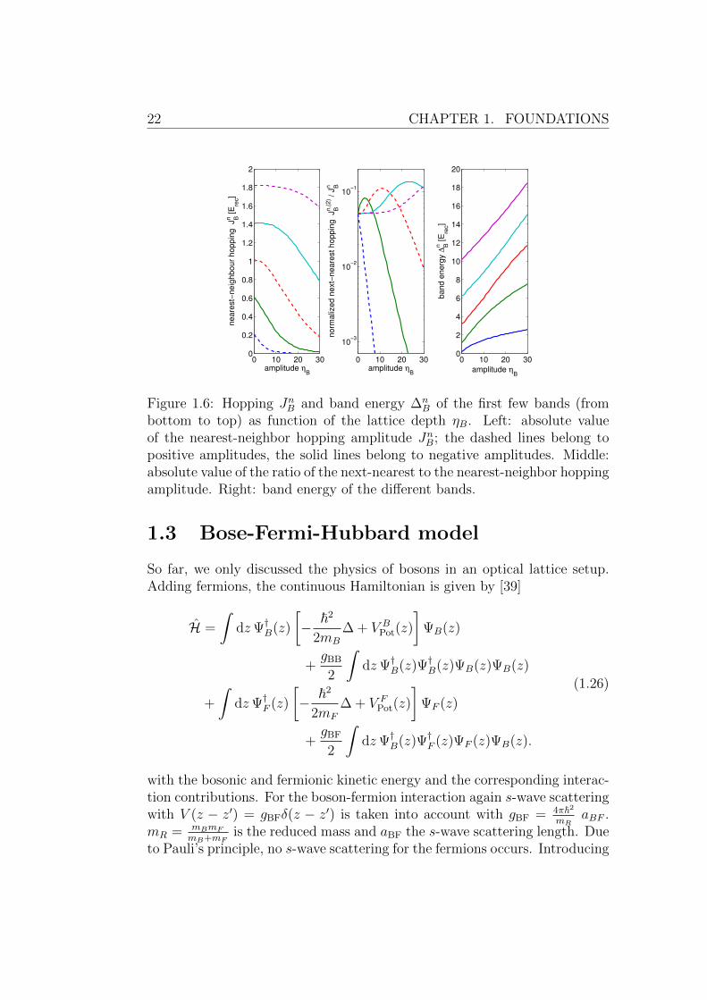
Figure 1.6 shows the calculated hopping amplitudes JnB and the band en-ergy ∆n
B as a function of the lattice amplitude ηB. Additionally, the ratio ofthe next-nearest to the nearest-neighbor hopping amplitude is shown. Thisproves, that the next-nearest hopping is small compared to the other quan-tities in the system and consistently left out.
22 CHAPTER 1. FOUNDATIONS
0 10 20 300
0.2
0.4
0.6
0.8
1
1.2
1.4
1.6
1.8
2
amplitude ηB
neare
st−
neig
hbour
hoppin
g J
Bn [E
rec]
0 10 20 30
10−3
10−2
10−1
amplitude ηB
norm
aliz
ed n
ext−
neare
st hoppin
g J
Bn,(
2) /
JBn
0 10 20 300
2
4
6
8
10
12
14
16
18
20
amplitude ηB
band e
nerg
y ∆
Bn [E
rec]
Figure 1.6: Hopping JnB and band energy ∆nB of the first few bands (from
bottom to top) as function of the lattice depth ηB. Left: absolute valueof the nearest-neighbor hopping amplitude JnB; the dashed lines belong topositive amplitudes, the solid lines belong to negative amplitudes. Middle:absolute value of the ratio of the next-nearest to the nearest-neighbor hoppingamplitude. Right: band energy of the different bands.
1.3 Bose-Fermi-Hubbard model
So far, we only discussed the physics of bosons in an optical lattice setup.Adding fermions, the continuous Hamiltonian is given by [39]
H =
∫dzΨ†B(z)
[− ~2
2mB
∆ + V BPot(z)
]ΨB(z)
+gBB
2
∫dzΨ†B(z)Ψ†B(z)ΨB(z)ΨB(z)
+
∫dzΨ†F (z)
[− ~2
2mF
∆ + V FPot(z)
]ΨF (z)
+gBF
2
∫dzΨ†B(z)Ψ†F (z)ΨF (z)ΨB(z).
(1.26)
with the bosonic and fermionic kinetic energy and the corresponding interac-tion contributions. For the boson-fermion interaction again s-wave scatteringwith V (z − z′) = gBFδ(z − z′) is taken into account with gBF = 4π~2
mRaBF .
mR = mBmF
mB+mFis the reduced mass and aBF the s-wave scattering length. Due
to Pauli’s principle, no s-wave scattering for the fermions occurs. Introducing

1.3. BOSE-FERMI-HUBBARD MODEL 23
Wannier functions for both, bosons [wB(z)] and fermions [wF (z)], we arriveat the Bose-Fermi-Hubbard model
H = −JB∑j
(a†j aj+1 + a†j+1aj
)+U
2
∑j
nj (nj − 1)− µB∑j
nj
− JF∑j
(c†j cj+1 + c†j+1cj
)+ V
∑j
njmj.(1.27)
mj = c†j cj is the fermionic number operator and c†j (cj) the fermionic creation(annihilation) operator. We included the chemical potential for the bosonsfor completeness, whereas we always fix the number of fermions, i.e., being ina semi-canonical description. The additional amplitudes in the Hamiltoniandescribe the fermionic kinetic energy
JF = −∫
dz wF (z − a)
[− ~2
2mF
∂2
∂z2+ V F
Pot(z)
]wF (z), (1.28)
and the local boson-fermion interaction
V =gBB
2
∫dz wB(z)wF (z)wF (z)wB(z). (1.29)
Here, we still restrict ourselves to nearest-neighbor hopping and local interac-tions. Again the bosonic interaction energy defines the energy scale by U = 1.
In general, we are not interested in the dependence of the different amplitudeson the lattice depth ηB, but discuss the influence of the different amplitudeson the system directly. Due to the four-dimensional3 parameter space ofthe Bose-Fermi-Hubbard model, an easy understanding of the model is notpossible. For several limiting cases, the prediction of various different phasesexist, partly verified by numerical means. Most prominent phases besidethe bosonic Mott insulators are paired or composite phases, polaritons andsupersolids [82, 83, 89, 117, 118, 119, 120] as well as studies on the influenceof disorder or superlattices on the Bose-Fermi-Hubbard model [121, 122, 123,124]. A more detailed discussion of the existing literature can be found inthe introductions to the different aspects of the Bose-Fermi-Hubbard model.
3Hoppings JB , JF , Bose-Fermi interaction V and bosonic chemical potential µB .

Part I
The Bose-Fermi-Hubbardmodel in the limit ofultraheavy fermions
25

CHAPTER 2
Introduction
Disorder in experimentally studied systems always affects the measurements,usually in a negative way. Nevertheless, disorder sometimes even enhancesphysical effects such as the conductance in graphene p-n junctions [125],the Curie temperature in the Anderson-Hubbard model [126, 127, 128],the synchronization of an array of Josephson junctions [129] or the phasecoherence [130]. Most prominent feature of the effect of disorder is thelocalization of non-interacting particles in a weak disordered potentialpredicted by Anderson [131]. Although being observed in a variety ofdifferent systems [132], ultracold atoms allowed for the first observation ofthe exponential localization [133, 134]. In addition to it, the full controlof ultracold atom systems opens the route to an understanding of theeffects of localization for interacting particles beyond Anderson localization[135, 136, 137].
In the (strongly) interacting regime, the so-called Bose glass is of im-portance [14, 109]. Partly possessing properties of the Mott insulator(no long-range phase coherence) and the superfluid (being compressible),the experimental search for the Bose glass in ultracold atoms reachedthe line with its observation in the excitation spectrum of cold atoms[71]. Further experiments studied the influence of the disorder on thecondensate fraction [106] or transport [138]. Theoretically, the Bose-glassphase is also found in systems without random on-site disorder but withdisorder in the interaction [139, 140] or the hopping amplitude [140, 141, 142].
Whereas in solid-state systems and other interesting models the nature andorigin of disorder cannot be controlled (beside doping), several implemen-
27
28 CHAPTER 2. INTRODUCTION
tations of the disorder are available in ultracold atoms. Superimposing theoptical lattice with a speckle pattern from a diffusive plate [69] and theinterference of two, non-commensurate optical lattices [71, 143, 144, 145, 146]are the easiest realizations of on-site disorder. Holographic methods used in[41] might also become interesting. The most intriguing source of disorder isthe usage of a second, immobile species. First studied in [147], this sourceof disorder quickly gained wide interest [148, 149, 150, Mering2008] withapplications to fermionic or bosonic impurities.
In this part of the thesis, we focus on the case of the Bose-Fermi-Hubbardmodel in the limit of immobile fermions, i.e., we consider the limit JF = 0.Here the effect of the fermions reduces to a binary random potential at sitej for the bosons, depending on whether a fermion is at a given site j or not.This means that the local bosonic chemical potential is altered by
δµj =
V, if a fermion is present at site j,0, otherwise.
(2.1)
The disorder distribution is thus given by ∆(x) = (1− %F )δ(x) + %F δ(x−V )with δ(x) being Dirac’s δ-function and V the boson-fermion interaction.The resulting model is closely related to the Falicov-Kimball model [151],describing the mixture of a mobile and an immobile fermionic species or theHubbard model with binary-alloy disorder [127, 152].
We systematically investigate to what extent this limit of the Bose-Fermi-Hubbard model can be described as a specific instance of a disordered Bose-Hubbard model with binary disorder and study the phase diagram which toour knowledge is not yet done1. This simple model shows important featuresof the full Bose-Fermi-Hubbard model but displays important qualitativedifferences to the phase diagram of the disordered Bose-Hubbard model withcontinuously distributed on-site disorder, as studied for instance in [14, 105,153, 154, 155]. Depending on the physical situation of interest, we considertwo cases of disorder: If the fermionic tunneling is small but sufficientlylarge such that on the time scales of interest relaxation to the state of totalminimum energy is possible, the fermion induced disorder is referred to asbeing annealed. In this case the ground state is determined by minimizationover all possible fermion distributions. If the fermion tunneling is too slowor the temperature too high the disorder is an actually random distributionwhich is then called quenched.
1Earlier studies mainly concentrated on the density-of-states and other quantities.
CHAPTER 3
Incompressible phases
3.1 Ultradeep lattices
We first discuss the phase diagram of the incompressible phases for the simplecase of an ultradeep lattice for the bosons, such that their hopping can beneglected. In this situation, where JF = JB = 0, the Hamiltonian becomesdiagonal in the occupation number basis, denoted as |n1,m1〉 · · · |nL,mL〉,where mj = 0, 1 is the number of fermions at site j and nj = 0, 1, ... thecorresponding number of bosons. L labels the total number of lattice sitesin the one-dimensional system. The problem of finding the ground statereduces to identifying product states with the lowest energy. By fixing thetotal number of fermions NF = L%F , where %F denotes the fermionic fillingfactor, this amounts to minimize
E =1
2
∑j
nj(nj − 1)− (µB − V )∑j∈F
nj − µB∑j∈N
nj. (3.1)
F denotes the set of %FL = NF sites with a fermion and N the set of(1 − %F )L = L − NF sites without a fermion. The energy is degenerate forall fermion distributions and the ground state is given by an equal mixtureof all states with state vectors
|ψ〉 =⊗i∈F
|n1, 1〉⊗j∈N
|n0, 0〉. (3.2)
Here,
n1 = max
0, [1/2 + (µB − V )], n0 = max
0, [1/2 + µB]
, (3.3)
29

30 CHAPTER 3. INCOMPRESSIBLE PHASES
is the local boson number for sites with (F) or without (N ) a fermion and[.] denotes the closest integer bracket. In other words, the degenerate stateswith lowest energy will have %FL sites with n1 bosons and one fermion andL(1− %F ) sites with n0 bosons and no fermion. For the case of unity (zero)fermion filling, %F = 1 (%F = 0), the situation becomes particularly simpleas we encounter the pure Bose-Hubbard model with an effective chemicalpotential µeff
B = µB − V (µB).
Since n1 and n0 are integers there are adjacent intervals of µ where the oc-cupation numbers do not change as it is the case in the plain Bose-Hubbardmodel. In these intervals the system is incompressible, i.e., the compressibil-ity vanishes. Following [83] we label the difference n0 − n1 in the bosonicnumber mediated through the presence of a fermion by s. The local groundstate can either consist of n0 bosons and no fermion or n1 = n0 − s bosonsand one fermion. These state vectors will be denoted as |n0, 0〉 = |0〉 and|n0 − s, 1〉 = |1〉. The value of s depends on µ and V and can be a positiveor negative integer. Both vectors are eigenvectors of the number operator
Qj = nj + smj (3.4)
with the same integer eigenvalue n0 and 〈∆Q2j〉 = 0. Thus incompressible
phases have a commensurate number Q and can be characterized by the twointegers n0 and s.
This behavior, illustrated in figure 3.1, is very similar to that of the Bose-Hubbard model except that here the bosons can be incompressible even fornon-integer filling %B since %B = n0+%F (n1−n0) [83, 156, Mering2008]. Sincen0 and n1 are integers and increase monotonically with µ, there is a jumpin the total number of bosons when moving from one incompressible phaseto the adjacent one. All systems with boson numbers between these valuesare critical and have the same chemical potential since JB = 0. The averageboson number per site in the incompressible phases does not have to bean integer, however. The existence of Mott phases with non-commensurateboson number is a direct consequence of the interaction of the bosons withthe fermions. At (random) sites with a fermion, the bosons experience aneffective local potential which resembles the physics of a disordered system.Due to the nature of this disorder, i.e., the occurrence of only two possiblevalues, the immobile fermions act as a binary disorder to the bosons. Asimilar behavior, i.e., the existence of non-integer incompressible lobes hasbeen shown for superlattices, which can be considered as binary disorder inthe special case of anti-clustering [157, Muth2008].

3.1. ULTRADEEP LATTICES 31
n = 0
n = 0
n = 1
n = 1
n = 2
n = 2
m = 0
V V
n = 0 n = 1 n = 2
n = 2 n = 3
V V V
m = 1
m = 0
n = 0 n = 1 n = 2
n = 1n = 0m = 1
m = 0
V
n =1, s=1 n =1, s=0 n =2, s=1 n =2, s=0
n =0, s=0 n =1, s=1 n =2, s=2 n =2, s=1
n =1, s=0 n =1, s=−1 n =2, s=0 n =2, s=−1
m = 1
µ 0 1−1/2 1/2 3/2 2
n =0, s=0
n =0, s=−1
0
n = 1
0 0
0 0
000
0
n = 0
n =0, s=00 0 0 0 0 0
0 0 0 0
00000
1 1 1 1
11
1 1 1
Figure 3.1: Phases of Bose-Fermi-Hubbard model for JB = JF = 0 fordifferent inter-species couplings 0 < V < 1 (lowest diagram), 1 < V < 2(middle diagram), −1 < V < 0 (upper diagram), and U = 1. n indicates thenumber of bosons (empty circles) at the site, m the number of fermions (redfilled circles). The horizontal red bars illustrate the boson number n1 for siteswith a fermion (m = 1) as function of the chemical potential, the horizontalblue bars correspondingly the boson number n0 for sites without a fermion(m = 0), which is identical to the Bose-Hubbard model. The values of µwhere a transition between different boson numbers n0 occurs are quantumcritical points.
In general Mott-insulating phases with incommensurate boson numbers existfor any disorder distribution that is non-continuous, i.e., containing a gapwithin the distribution. This stems from the fact, that the different disordervalues account to a shift of the JB = 0 phase diagram of the Bose-Hubbardmodel. For a gapped disorder distribution, these shifts leave regions withthe same number of bosons open, as seen in figure 3.1 for the binary disorderdistribution. In this sense, also the behavior of the non-integer Mott lobesfor arbitrary superlattices can be understood.

32 CHAPTER 3. INCOMPRESSIBLE PHASES
3.2 Minimum energy distribution of fermions
for small bosonic hopping
In order to understand the physics of disorder due to the presence offermions we need to discuss the influence of the distribution of fermionsto the ground-state energy. The energetic degeneracy of different fermiondistributions in the incompressible phases is lifted if a small bosonic hoppingJB is taken into account. Near the quantum critical points the bosonhopping leads to the formation of possibly critical phases with growingextent. We first restrict ourselves to regions where incompressibility ismaintained, i.e., sufficiently far away from the critical points.
In order to obtain a qualitative understanding of the effects of a finitebosonic hopping we performed a numerical perturbation calculation on asmall lattice. Figure 3.2 shows different distributions of 4 fermions over alattice of 8 sites ordered according to their energy for different parametersin 6th order perturbation.
One notices that the lowest energy states are either given by fermion dis-tributions with maximum mutual distance (anti-clustered configuration) orminimum mutual distance (clustered configuration) modified by boundaryeffects. This behavior can in part be explained by a composite fermion pic-ture introduced in [83]. The composite fermions are defined for the phase(n0, s) by the annihilation operators
fi =
√(n0 − s)!n0!
(b†i
)sci, for s ≥ 0 (3.5)
fi =
√n0!
(n0 − s)!
(bi
)−sci, for s < 0, (3.6)
and describe the fermions surrounded by a bosonic (bosonic hole) cloud ontop of a boson see. For details, refer to [83].
For each (n0, s), the full Bose-Fermi-Hubbard Hamiltonian (1.27), withJF = 0 gives, in second order in JB, rise to an effective Hamiltonian[83, 121, 158, 159, 160]
Heff = Keff
∑〈i,j〉
(f †i fi)(f†j fj). (3.7)

3.2 MINIMUM ENERGY DISTRIBUTION 33
Figure 3.2: Fermion distributions ordered increasingly by ground-state en-ergy for JF = 0, JB = 0.02, U = 1. The energy ranges from small (blue) tolarger (red) values. Top: attractive boundary, left: (V, n0, s) = (1, 1), i.e.,Keff = −0.002, and right: (1.5, 2, 1), i.e., Keff = 0.001. Bottom: repulsiveboundary, left: (−1.5, 0,−1), i.e., Keff = −0.002, right: (−1.5, 1,−1), i.e.,Keff = 0.001. For the definition of Keff refer to equation (3.8).

34 CHAPTER 3. INCOMPRESSIBLE PHASES
The effective coupling (note that U = 1 and JF = 0 in contrast to [83]) reads
Keff = 4J2B
[n0(n0 + 1− s)1− s+ V
+(n0 − s)(n0 + 1)
1 + s− V− n0(n0 + 1)− (n0 − s)(n0 + 1− s)
]. (3.8)
Composite fermions cannot occupy the same lattice site, but there is anearest-neighbor attraction (Keff < 0) or repulsion (Keff > 0), dependingon (n0, s) and V . Associating a site with a composite fermion with aspin-up state and a site without a fermion with spin down, equation (3.8)corresponds to the classical Ising model with fixed magnetization andanti-ferromagnetic (Keff > 0) or ferromagnetic coupling (Keff < 0). At thispoint it should be mentioned, that introduction of the composites doesnot explain important properties of the system. As pointed out in ourprevious work [161, Mering2008], the fluctations of the composite numberoperator are non-zero which cannot be seen from the effective Hamiltonian(3.8). Nevertheless it gives an effective understanding of the behavior of thefermions in the system.
As a consequence, if Keff < 0, the energy is smallest for composite (andtherefore fermion) distributions that minimize the surface area of siteswith and without a fermion (referred to as clustering). In this setting, thefermion distribution forms a block of occupied sites. For this block, theopen boundary condition either yields attractive or repulsive interactionwith the boundary which explains the behavior of the energy of the differentdistributions in figure 3.2. If s > 0, the boundaries are attractive, otherwiserepulsive as seen in the figure.
The other regime is the one for Keff > 0. Then, the fermions repel eachother and form a pattern with maximum number of boundaries for small JB,referred to as anti-clustering. The fact that the fermions attain a distributionwith maximum distance cannot be explained by the effective model due toits perturbative nature. In all of our numerical simulations using DMRGwe found however that a positive Keff always leads to anti-clustering withmaximum distance. This behavior of clustering and anti-clustering is alsoreported in [83, 162] for slightly different parameters JF .
From figure 3.2, another important feature can be seen. As the colorcode shows, the energies for the different distributions differ only bya small amount on the order of J2
B/U or even higher orders n. Thismeans, that for temperatures which are still small enough to treat the
3.2 MINIMUM ENERGY DISTRIBUTION 35
3210
2
4
6
8
10
0
0.1
0.2
0.3
s
n0
−1−2−30
2
4
6
8
10
0
0.1
0.2
0.3
s
n0
Keff
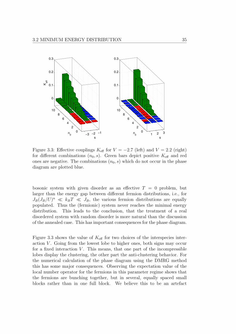
Figure 3.3: Effective couplings Keff for V = −2.7 (left) and V = 2.2 (right)for different combinations (n0, s). Green bars depict positive Keff and redones are negative. The combinations (n0, s) which do not occur in the phasediagram are plotted blue.
bosonic system with given disorder as an effective T = 0 problem, butlarger than the energy gap between different fermion distributions, i.e., forJB(JB/U)n kBT JB, the various fermion distributions are equallypopulated. Thus the (fermionic) system never reaches the minimal energydistribution. This leads to the conclusion, that the treatment of a realdisordered system with random disorder is more natural than the discussionof the annealed case. This has important consequences for the phase diagram.
Figure 3.3 shows the value of Keff for two choices of the interspecies inter-action V . Going from the lowest lobe to higher ones, both signs may occurfor a fixed interaction V . This means, that one part of the incompressiblelobes display the clustering, the other part the anti-clustering behavior. Forthe numerical calculation of the phase diagram using the DMRG methodthis has some major consequences. Observing the expectation value of thelocal number operator for the fermions in this parameter regime shows thatthe fermions are bunching together, but in several, equally spaced smallblocks rather than in one full block. We believe this to be an artefact
36 CHAPTER 3. INCOMPRESSIBLE PHASES
of the build-up mechanism (for details see [163]) in the DMRG code1,which nevertheless does not limit the applicability of our results. Morerecent implementations of the DMRG method without finite size build-up[167, 168, 169] could perhaps overcome this problem.
3.3 Incompressible phases for finite JB
For finite bosonic hopping JB we extend the strong-coupling expansionapplied in [97] to the Bose-Hubbard model and complement the resultswith numerical DMRG simulations. This formulation of the strong-couplingexpansion provides a rather accurate description of the Bose-Hubbardmodel even on a quantitative level, with further improvements from theemployment of a field theoretic approach [170, 171, 172, 173].
In the zero hopping limit JB = 0, all fermion distributions give the sameenergy. Considering the phase with (n0, s) and NF = %FL fermions, theground-state vector is found to be
∣∣ψ⟩ =⊗j∈F
c†j(a†j)(n0−s)√
(n0 − s)!
⊗k∈N
(a†k)n0
√n0!|0〉, (3.9)
where |0〉 = |0, . . . , 0〉B ⊗ |0, . . . , 0〉F is the total vacuum of both bosons andfermions at all sites. The energy density is given by
ε0 =U
2
[(1− %F )n0(n0 − 1) + %F (n0 − s)(n0 − s− 1)
]+ V %F (n0 − s).
For a state with a single additional boson (bosonic hole), we have todistinguish two cases compared to the usual Bose-Hubbard model. Firstthe boson (bosonic hole) can be added to a site with a fermion, or second,without a fermion. Up to normalization, we have
1The DMRG code used was provided by Prof. Dr. U. Schollwock. Unfortunately,the code does not allow to change the intrinsic routines to get rid of unwanted effects.This prevented us to study further interesting quantities in the system. Nevertheless,all important physical quantities calculated using the DMRG code are sufficient for thestudy and prediction of the new phases described throughout the whole work. The usageof open-source program packages as the ALPS [164, 165] or PwP [166] projects is notpossible since these are not yet implemented for Bose-Fermi mixtures.
3.3. INCOMPRESSIBLE PHASES FOR FINITE JB 37
∣∣ψ+F⟩j
= a†j∣∣ψ0
⟩,
∣∣ψ−F⟩j = aj∣∣ψ0
⟩, for j ∈ F , (3.10)
for sites with a fermion and∣∣ψ+N⟩j
= a†j∣∣ψ0
⟩,
∣∣ψ−N⟩j = aj∣∣ψ0
⟩, for j ∈ N , (3.11)
for sites without a fermion. All of these vectors are eigenvectors of the Bose-Fermi-Hubbard Hamiltonian for JB = 0 with respective energies
E+F = E0 + V + U(n0 − s), E+
N = E0 + Un0, (3.12)
E−F = E0 − V + U(n0 − s− 1), E−N = E0 + U(n0 − 1), (3.13)
where E0 = Lε0. The corresponding chemical potentials read
µ+F = E+
F − E0 = V + U(n0 − s), (3.14)
µ−F = E0 − E−F = µ+F − U,
and
µ+N = E+
N − E0 = Un0, (3.15)
µ−N = E0 − E−N = µ+N − U.
Except from the special case V = Us, the energies E±F and E±N all differfrom each other. Thus we can determine the phase boundaries for JB 6= 0by degenerate perturbation theory within the subspaces with the additionalboson (bosonic hole) in sites j ∈ F or j ∈ N separately.
There will be a second order contribution in JB for sites j that have atleast one neighboring site of the same type. For isolated sites degenerateperturbation theory will lead only to higher order terms in JB. Since theboundaries of the incompressible phases are determined by the overall lowest-energy particle-hole excitations, we can construct the expected phase diagramin the case of extended connected regions of fermion sites coexisting withextended connected regions of non-fermion sites. In this case we can directlyapply the results of [97] to sites with and without fermions yielding
µ±F/N = µ±F/N + δµ±(n0, JB) (3.16)
where
δµ+(n0, JB) = −2JB(n0 + 1) + J2Bn
20 + J3
Bn0(n0 + 1)(n0 + 2),
δµ−(n0, JB) = 2JBn0 − J2B(n0 + 1)2 − J3
Bn0(n20 − 1).
(3.17)

38 CHAPTER 3. INCOMPRESSIBLE PHASES
Figure 3.4: Phase diagram from strong-coupling expansion withU = 1, V = 1.5. Red areas (A) indicate truly incompressible Mott regionswith gapped particle-hole excitations everywhere. Green (B) and blue (C)areas are partially compressible quasi-Mott regions with gapped particle-holeexcitation for sites with (B) or without (C) a fermion but ungapped excita-tion in the complementary region. Outside the three regions, the system iscompletely compressible.
This gives rise to two overlapping sequences of the usual Mott-insulatinglobes, one for the sites with and one for the sites without fermions. Accord-ing to (3.14), the shift is given by the boson-fermion interaction V and theeffect on the phase diagram is shown in figure 3.4. In [149], similar resultsincluding higher dimensions can be found.
As seen in the figure, the system is truly incompressible only in the overlapregion (A) of the quasi-Mott lobes for sites with and without fermions.Points which are within one of the two sequences of quasi-Mott lobes butnot in both (cases B or C) are not compressible in the whole system butonly in a region. Thus the energy for a particle-hole excitation is gappedwithin this sublattice and ungapped in the other part upon addition of aboson (bosonic hole). Outside the three described regions, the system isfully compressible. It should be mentioned that a similar procedure allowsto describe the phases in the (general) disordered Bose-Hubbard model,which can have many shifted Bose-Hubbard phase diagrams overlapping,also explaining the emergence of non-integer incompressible phases for weak,gapped disorder.

3.3. INCOMPRESSIBLE PHASES FOR FINITE JB 39
The analytic result (3.17) for the different phases allows for a directcomparison to numerical results from DMRG. Therefore we employ DMRGwith open boundary conditions and two different fermionic distributions,the clustered and the anti-clustered one. Throughout the whole thesis, thelocal dimension of the Hilbert space in the DMRG as well as the dimensionof the blocks are chosen in such a way, that no significant change in thenumerical results upon increasing the two quantities could be observed.Figure 3.5 shows the corresponding numerical results together with theanalytic prediction from (3.17). For the phase diagrams throughout thispart, a finite size extrapolation (see section 3.4 and [107]) is performed.
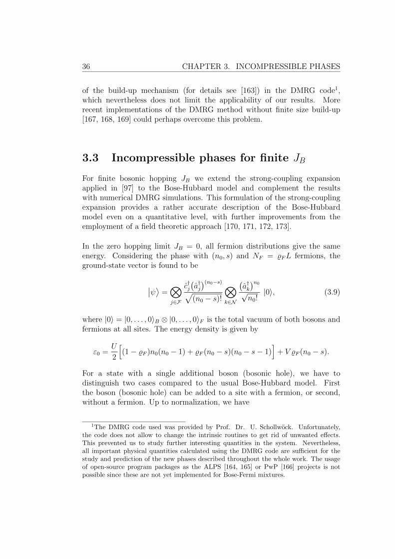
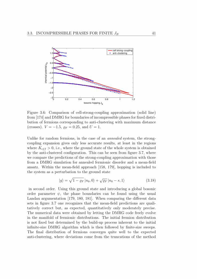
One recognizes nearly perfect agreement between numerics and strong-coupling prediction in the case of clustering. This is expected since in theclustered case the majority of sites has neighbors of the same type. Inthe case of anti-clustering, however, the incompressible lobes extend muchfurther into the region of large boson hopping with a critical JB of about 1for a fermion filling of %F = 0.25 at V = −1.5. This behavior is expectedsince in this case hopping to nearest-neighbors is suppressed if the neigh-boring sites are of a different type (F or N ). For this situation, the curvesof the critical chemical potential µcrit(JB) that correspond to a bosonicparticle-hole excitation at a fermion site (here µcrit(0) = −1.5,−0.5, 0.5, 1.5etc.) start with a power JγB determined by the minimum number of hopsrequired to reach the next fermion site, i.e., γ = 1/ρF , if %F ≤ 1/2. If thefermion filling is larger than 1/2 the behavior changes and the non-fermionsites (hole sites) cause µcrit(JB) ∼ JγB with γ = 1/(1 − %F ). In principleit is possible to extend the strong-coupling perturbation expansion to anyfermion distribution (compare the method presented in section C.1), which ishowever involved. In [175, 176] a numerically assisted strong-coupling theorytermed cell-strong-coupling expansion is developed. Since the anti-clusteredsituation is equivalent to the Bose-Hubbard model with a superlattice, thesemi-analytic results from this method can be applied directly. Figure 3.6shows a comparison of the numerical results using DMRG from figure 3.5for V = −1.5 to the results from the cell-strong-coupling approach2 showinga very good agreement as expected3.
2Thanks to P. Buonsante for the cell-strong-coupling results of the phase boundaries.3It should be noted that the loop-hole insulator phases [174, 177, 178, Muth2008]
predicted for a super-lattice are for the present parameters too small to be visible in theDMRG simulation and are nevertheless expected to disappear after averaging over disorderdistributions.

40 CHAPTER 3. INCOMPRESSIBLE PHASES
0 0.05 0.1 0.15 0.2 0.25 0.3 0.35−1
−0.5
0
0.5
1
1.5
2
2.5
3
bosonic hopping JB
ch
em
ica
l p
ote
ntia
l µ
B
analytic
clustering
anti−clustering
V=1.5
0 0.1 0.2 0.3 0.4 0.5 0.6 0.7 0.8 0.9 1−2.5
−2
−1.5
−1
−0.5
0
0.5
1
1.5
2
bosonic hopping JB
ch
em
ica
l p
ote
ntia
l µ
B
analytic
clustering
anti−clustering
V=−1.5
Figure 3.5: Comparison of the incompressible phases predicted from thestrong-coupling approximation (solid line) to DMRG results (circles,crosses)for two fixed distributions of fermions. Circles: clustering, Crosses: anti-clustering with maximal distance. V = 1.5 (top figure) and V = −1.5(bottom figure). %F = 0.25, and U = 1.
So far we did not discuss the issue of fermionic distributions which areunequal the two cases. For the situation of random disorder, i.e., a fixedfermionic distribution, the so-called rare events [97, 155] are of majorimportance to the phase diagram. In the thermodynamic limit, all possibledisorder configurations appear within the system; in particular also theoptimal situation of a large clustered region. Here, optimal is used inthe sense that the superfluid to Mott-insulator transition occurs in thisconfiguration first. Thus our strong-coupling results describe the phasediagram properly for binary disorder in the thermodynamic limit becausethe clustered distribution is always the optimal one.
3.3. INCOMPRESSIBLE PHASES FOR FINITE JB 41
0 0.2 0.4 0.6 0.8 1 1.2−3
−2.5
−2
−1.5
−1
−0.5
0
0.5
1
1.5
2
bosonic hopping JB
chem
ical pote
ntial µ
B
cell strong−coupling
anti−clustering
Figure 3.6: Comparison of cell-strong-coupling approximation (solid line)from [174] and DMRG for boundaries of incompressible phases for fixed distri-bution of fermions corresponding to anti-clustering with maximum distance(crosses). V = −1.5, %F = 0.25, and U = 1.
Unlike for random fermions, in the case of an annealed system, the strong-coupling expansion gives only less accurate results, at least in the regionswhere Keff > 0, i.e., where the ground state of the whole system is obtainedby the anti-clustered configuration. This can be seen from figure 3.7, wherewe compare the predictions of the strong-coupling approximation with thosefrom a DMRG simulation for annealed fermionic disorder and a mean-fieldansatz. Within the mean-field approach [158, 179], hopping is included tothe system as a perturbation to the ground state
|g〉 =√
1− %F |n0, 0〉+√%F |n0 − s, 1〉 (3.18)
in second order. Using this ground state and introducing a global bosonicorder parameter ψ, the phase boundaries can be found using the usualLandau argumentation [179, 180, 181]. When comparing the different datasets in figure 3.7 one recognizes that the mean-field predictions are quali-tatively correct but, as expected, quantitatively only moderately precise.The numerical data were obtained by letting the DMRG code freely evolvein the manifold of fermionic distributions. The initial fermion distributionis not fixed but determined by the build-up process inherent to the initialinfinite-size DMRG algorithm which is then followed by finite-size sweeps.The final distribution of fermions converges quite well to the expectedanti-clustering, where deviations come from the truncations of the method

42 CHAPTER 3. INCOMPRESSIBLE PHASES
0 0.05 0.1 0.15 0.2 0.25 0.3−0.5
0
0.5
1
1.5
2
2.5
3
bosonic hopping JB
chem
ical pote
ntial µ
B
strong−couplingmean fieldDMRG
Figure 3.7: Incompressible phases for annealed fermions and U = 1,V = 0.25, %F = 0.25. Within the incompressible phases, the final fermiondistributions correspond to the totally anti-clustered state, in agreement withthe analytic predictions of section 3.2. Shown are the strong-coupling results(solid line), the mean-field results from [179] (dashed line) and results froma DMRG calculation with JF = 0 (crosses) for annealed fermions.
and the complex energy manifold with many metastable low-energy states.Since the DMRG method is prone to get stuck in local minima we checkedthe consistency of our results by implementing different sweep algorithmsafter the initial infinite size algorithm. In these sweep algorithms, thefermionic hopping was not taken to be zero but was given a finite initialvalue which was decreased during the DMRG sweeps to the final value zero.To ensure proper convergence we compared the data for a few representativepoints (JB = 0.07 boundaries of (n0, s) = (1, 1) lobe; JB = 0.15 boundariesof (1, 0) lobe; JB = 0.03 boundaries of (2, 0) lobe) to the data obtained fromtwo different sweep strategies4. The difference in the chemical potential isof the order of 3% independent of the sweep strategy an therefore negligibleon the scale of the plot. It should be noted, that the build-up procedure
4 The sweep strategy was implemented by first applying an infinite size algorithm up tothe system length, then applying 5 finite size sweeps, all at JF = JB/2. Subsequently thehopping was reduced after a complete sweep and again 3 sweeps were carried out to ensureconvergence again with the new hopping amplitude. Repeatedly, the hopping was slightlyreduced until after 30 sweeps the fermionic hopping is set to be 0 with another 3 sweeps.In the first method the hopping was reduced according to an exponential decay followedby a linear decay to zero. In the second method the hopping was reduced according to acosine followed by a linear decay to zero.
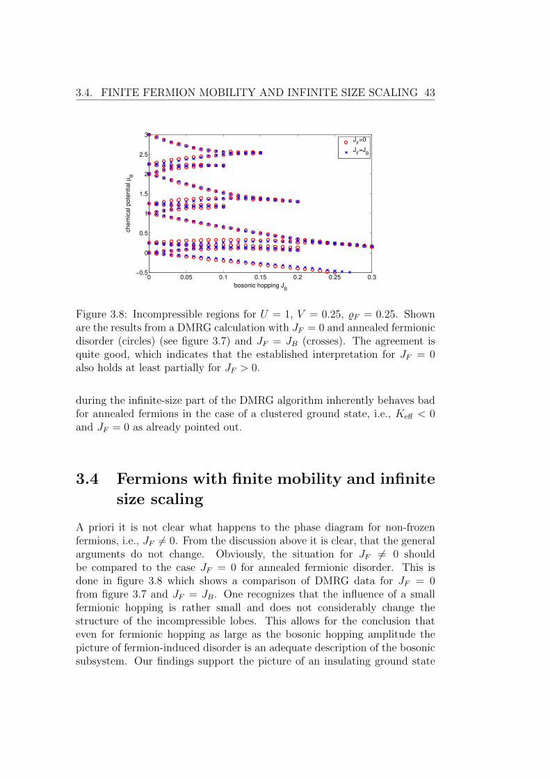
3.4. FINITE FERMION MOBILITY AND INFINITE SIZE SCALING 43
0 0.05 0.1 0.15 0.2 0.25 0.3−0.5
0
0.5
1
1.5
2
2.5
3
bosonic hopping JB
chem
ical pote
ntial µ
B
JF=0
JF=J
B
Figure 3.8: Incompressible regions for U = 1, V = 0.25, %F = 0.25. Shownare the results from a DMRG calculation with JF = 0 and annealed fermionicdisorder (circles) (see figure 3.7) and JF = JB (crosses). The agreement isquite good, which indicates that the established interpretation for JF = 0also holds at least partially for JF > 0.
during the infinite-size part of the DMRG algorithm inherently behaves badfor annealed fermions in the case of a clustered ground state, i.e., Keff < 0and JF = 0 as already pointed out.
3.4 Fermions with finite mobility and infinite
size scaling
A priori it is not clear what happens to the phase diagram for non-frozenfermions, i.e., JF 6= 0. From the discussion above it is clear, that the generalarguments do not change. Obviously, the situation for JF 6= 0 shouldbe compared to the case JF = 0 for annealed fermionic disorder. This isdone in figure 3.8 which shows a comparison of DMRG data for JF = 0from figure 3.7 and JF = JB. One recognizes that the influence of a smallfermionic hopping is rather small and does not considerably change thestructure of the incompressible lobes. This allows for the conclusion thateven for fermionic hopping as large as the bosonic hopping amplitude thepicture of fermion-induced disorder is an adequate description of the bosonicsubsystem. Our findings support the picture of an insulating ground state

44 CHAPTER 3. INCOMPRESSIBLE PHASES
512 128 64 48 32 24 16 120.04
0.06
0.08
0.1
0.12
0.14
0.16
0.18
system size L
critical hoppin
g J
Bc
Figure 3.9: Thermodynamic limit extrapolation for the critical point of then0 = 1, s = 1 lobe (%F = 0.25, %B = 0.75) in figure 3.8. The critical point isfound at J cB = 0.16038
developed in [182]
As final property of the incompressible phases we study the behavior of thecritical hopping amplitude of one lobe as a function of the system size. Infinite size numerical situations, boundary effects are always present when us-ing open boundary conditions. As example, in the finite system the spectrumis always gapped, even within the superfluid phase. Considering free bosons,described by the Hamiltonian
H = −JB∑j
(a†j aj+1 + a†j+1aj
), (3.19)
the energy cost per particle is proportional to 1/L, with L being the systemsize. For the calculation of the tip of the Mott insulators, a finite size scalingin 1/L turns out to be suitable to obtain the infinite size limit [183]. Ex-emplarily we study the finite size scaling of the lowest lobe (n0, s) = (1, 1)in figure 3.8 for JF = JB. Figure 3.9 shows the critical point calculatedfrom DMRG for various system sizes as function of 1/L. From a fit of J cB tolog(L) we find the critical point in the thermodynamic limit Jc = 0.16038.The data for different system lengths show the expected 1/L behavior forthe Bose-Hubbard model [183].
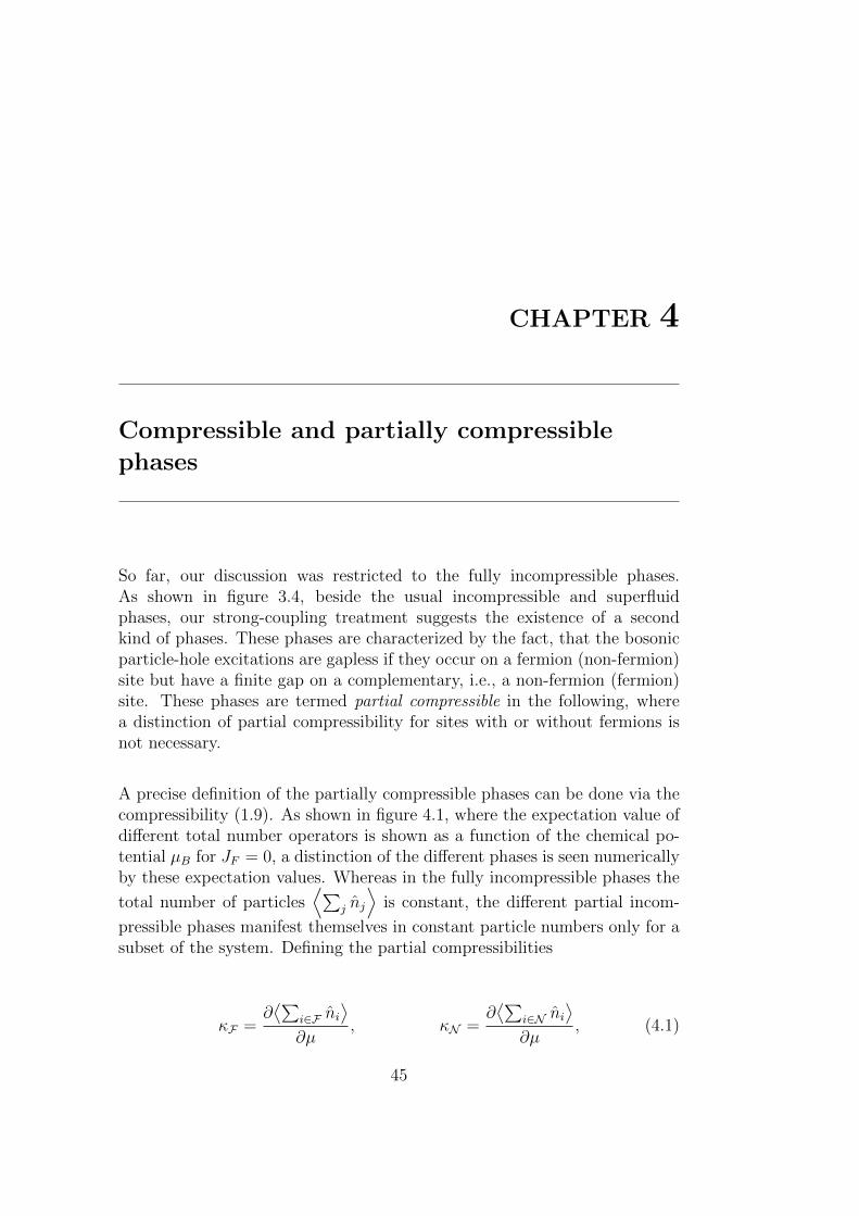
CHAPTER 4
Compressible and partially compressible
phases
So far, our discussion was restricted to the fully incompressible phases.As shown in figure 3.4, beside the usual incompressible and superfluidphases, our strong-coupling treatment suggests the existence of a secondkind of phases. These phases are characterized by the fact, that the bosonicparticle-hole excitations are gapless if they occur on a fermion (non-fermion)site but have a finite gap on a complementary, i.e., a non-fermion (fermion)site. These phases are termed partial compressible in the following, wherea distinction of partial compressibility for sites with or without fermions isnot necessary.
A precise definition of the partially compressible phases can be done via thecompressibility (1.9). As shown in figure 4.1, where the expectation value ofdifferent total number operators is shown as a function of the chemical po-tential µB for JF = 0, a distinction of the different phases is seen numericallyby these expectation values. Whereas in the fully incompressible phases the
total number of particles⟨∑
j nj
⟩is constant, the different partial incom-
pressible phases manifest themselves in constant particle numbers only for asubset of the system. Defining the partial compressibilities
κF =∂⟨∑
i∈F ni⟩
∂µ, κN =
∂⟨∑
i∈N ni⟩
∂µ, (4.1)
45

46 CHAPTER 4. COMPRESSIBLE PHASES
chemical potential µB
avera
ge d
ensitie
s
−0.2 0 0.2 0.4 0.6 0.8 1 1.2 1.4 1.60
0.25
0.75
1
1.25
1.75
2
−0.1 0 0.1 0.20
0.25
0.75
1
Figure 4.1: Density cut along the µB-axis in figure 3.8 for JF = 0 (annealed)and JB = 0.02, U = 1, V = 0.25, %F = 0.25. From top to bottom: over-
all average density⟨∑
j nj
⟩, average density for sites without a fermion⟨∑
j∈N nj
⟩and average density for sites with a fermion
⟨∑j∈F nj
⟩, all after
averaging as described in the main text. Inset: Dependence of the particlenumber as function of chemical potential without averaging. The system sizeis chosen to be L = 128 sites. Gray background indicates the regions of thefull incompressible phases, i.e., the quasi-Mott insulators.
the two different phases from figure 3.4 are
B: κF = 0 κN 6= 0
C: κF 6= 0 κN = 0.(4.2)
Within each of the partial compressible phases, all additional particles enterthe sublattices denoted F or N , depending on the chemical potential.
For vanishing fermionic hopping, the results for the different number ofparticles in the subset of the lattice are displayed in figure 4.1. Here theaverage boson number per site obtained from a DMRG simulation withannealed disorder is shown as a function of the chemical potential forJB = 0.02. Also shown are the corresponding values only for fermion sitesand non-fermion sites respectively. In the partially compressible phases theaverage boson number increases only for one type of sites while it staysconstant for the other. As seen in the inset of the figure, the chemicalpotential is not a monotonous function of the filling as it should be. This

CHAPTER 4. COMPRESSIBLE PHASES 47
artefact of the numerical method in this highly demanding parameter regimeis overcome by an averaging of the chemical potential of a small number ofdifferent fillings. These averaged results are shown in the main part of thefigure. As mentioned earlier, the problem stems from the complex energysurface in the parameter space and the trapping of the numerical algorithmin metastable states close to the ground state.
We now discuss the properties of the single-particle density matrix 〈a†i ai+m〉in the partially incompressible phases. In general, for very large values of JBthe system is expected to have a Luttinger-liquid behavior [184, 185, 186]in one dimension with 〈a†i ai+m〉 ∼ m−K/2 and to possess long-range off-diagonal order in higher dimensions. K is the so-called Luttinger parameterwhich is essential for the understanding of the existing phases. In onedimension, we expect the Luttinger-liquid behavior to disappear in thepartially incompressible phases and correlations to decay exponentially as〈a†i ai+m〉 ∼ e−m/Lc . This is because in this case a single (static) impurity issufficient to prevent the build-up of long-range correlations. This accountsfor a percolation problem, where for higher dimensions there will be acritical fermion (or hole) filling above which off-diagonal order is suppressed.This critical filling is determined by percolation thresholds and for annealedfermionic disorder depends on the actual fermion distribution in theground state (e.g. clustered or anti-clustered). For a (quenched) randomfermion distribution in two dimensions, the threshold is %crit
F = 0.5927 (or1− %crit
F = 0.5927 if non-fermion sites are incompressible) and %critF = 0.3116for three dimensions [187]. See [188] for the percolation threshold of avariety of two-dimensional lattices.
Figure 4.2 shows the first-order correlations 〈a†i ai+m〉 as function of thedistance m for an annealed fermion distribution obtained from DMRGsimulations for a rather large lattice of 512 sites with incommensurate bosonfilling (NB = 448) and %F = 0.25. i and i + m are chosen symmetricallyaround the center. For JB = 0.07, strong exponential decay with correlationlength Lc = 1.3 is found corresponding to a glass-type behavior (due to thefinite compressibility), while for JB = 0.2 correlations decay algebraicallywith 〈a†i ai+m〉 ∼ m−0.32, which corresponds to a Luttinger liquid. TheLuttinger parameter K = 0.64 is slightly smaller than the known valuefor the critical point of the superfluid to Bose-glass transition K = 2/3[109] with box-disorder thus being close to the transition. It should bementioned that so far it is not clear whether the result for the superfluid toBose-glass transition for boxed disorder, i.e., a disorder distribution with∆(x) = 1
∆Θ(∆ − x)Θ(x) is applicable also for the binary disorder with
48 CHAPTER 4. COMPRESSIBLE PHASES
64 128 192 256 320 384 448 51210
−15
10−10
10−5
100
DMRG
exponential fit
32 64 128 256 512
10−1
100
distance m
firs
t−ord
er
corr
ela
tion <
aj+ a
j+m
>
DMRG
algebraic fit
exp(−m/1.3)
m−0.32
JB=0.2
JB=0.07
Figure 4.2: DMRG simulations (crosses) of first-order correlations 〈a†i ai+m〉for V = 0.25, %F = 0.25 and U = 1 for a lattice of L = 512 sites andNB = 448bosons in the case of annealed disorder. Top: Within the partial compressiblephase (JB = 0.07), the line corresponds to the exponential fit ∼ exp−m/Lcwith Lc = 1.3. The exponential decay is apparent. Bottom: Superfluidregion (JB = 0.2), the line corresponds to the algebraic fit ∼ m−K/2 with theexponent K = 0.64.
∆(x) = (1−%F )δ(x)+%F δ(x−V ) case. Nevertheless it serves as a rough esti-mate. Another evidence for the existence of a glass-like phase in this systemis seen in [189], where the superfluid fraction is calculated from a Gutzwillerapproach. This study shows the existence of a region outside the Mott in-sulators with zero compressibility, indicating the partial compressible phases.
The phases in figure 3.4 display another uncommon feature. Since theearly work of Fisher et al. [14] and an (incomplete) DMRG study by Paiet al. [190], the question of the nature of the phase transition at the tip ofthe lobe for boxed disorder stayed open. Different scenarios were discussed,distinguishing between a direct superfluid to Mott-insulator transitioneven for ∆ > 0 or the existence of an intermediate Bose-glass phase.Though numerical [105] and analytic results [97] favored the existence ofan intermediate Bose-glass phase, the strict proof was only found recentlyby Pollet et al. for the case of generic, bounded disorder [191, 192]. Forour situation of a binary disorder distribution, the strong-coupling resultssuggest the existence of a direct superfluid to Mott-insulator transition. Afinal, decisive answer to this question related to the nature of our disorder

CHAPTER 4. COMPRESSIBLE PHASES 49
16 32 48 64 80 96 112 12810
−15
10−10
10−5
100
DMRG
exponential fit
8 16 32 64 12810
−1
100
distance m
firs
t−ord
er
corr
ela
tion <
aj+ a
j+m
>
DMRG
algebraic fit
exp(−m/2)
m−0.21
JB=0.2
JB=0.03
Figure 4.3: DMRG simulations (crosses) of first-order correlations 〈a†i ai+m〉for V = 1.5, %F = 0.375 and U = 1 for a lattice of L = 128 sites andNB = 184 bosons, averaged over 100 fermion distributions. Top: JB = 0.03,the line corresponds to the exponential fit ∼ exp−m/Lc with Lc = 2. Theexponential decay is apparent. Bottom: JB = 0.2, the line corresponds tothe algebraic fit ∼ m−K/2 with the exponent K = 0.42. To avoid finite sizeeffects at short and long ranges, the fitting is done only for intermediatedistances.
distribution can however not be given at this point.
Figure 4.3 shows the first-order correlations for random, quenched fermiondistribution averaged over 100 realizations with non-commensurate bosonnumber (%B = NB/N = 184/128). Despite the sampling noise one recognizesthe transition between exponential decay with correlation length Lc = 2 forJB = 0.03, and a power-law decay with m−0.21 for JB = 0.2 correspondingto a Luttinger liquid with K = 0.42. JB = 0.03 is within a partiallyincompressible phase, JB = 0.2 outside, proving that our picture of partiallycompressible phases holds in both cases, annealed and quenched disorder.
Numerical results for the situation of non-vanishing but small fermionic hop-ping reveal that (strict) partial incompressibility is lost. But still the increaseof the boson number with increasing chemical potential at one type of sitesis substantially less that that on the complementary type of sites:
κF κN or κN κF . (4.3)
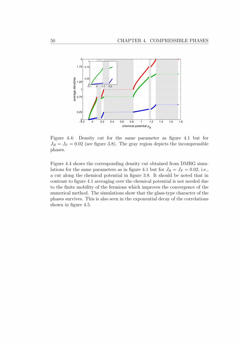
50 CHAPTER 4. COMPRESSIBLE PHASES
chemical potential µB
avera
ge d
ensitie
s
−0.2 0 0.2 0.4 0.6 0.8 1 1.2 1.4 1.6 1.80
0.25
0.75
1
1.25
1.75
2
−0.1 0 0.1 0.20
0.25
0.75
1
Figure 4.4: Density cut for the same parameter as figure 4.1 but forJB = JF = 0.02 (see figure 3.8). The gray region depicts the incompressiblephases.
Figure 4.4 shows the corresponding density cut obtained from DMRG simu-lations for the same parameters as in figure 4.1 but for JB = JF = 0.02, i.e.,a cut along the chemical potential in figure 3.8. It should be noted that incontrast to figure 4.1 averaging over the chemical potential is not needed dueto the finite mobility of the fermions which improves the convergence of thenumerical method. The simulations show that the glass-type character of thephases survives. This is also seen in the exponential decay of the correlationsshown in figure 4.5.

CHAPTER 4. COMPRESSIBLE PHASES 51
16 32 48 64 80 96 112 128
10−2
100
DMRG
exponential fit
8 16 32 64 128
10−2
100
distance m
firs
t−ord
er
corr
ela
tion <
aj+ a
j+m
>
DMRG
exponential fit
exp(−m/1.8)
JB=J
F=0.02
JB=J
F=0.02
Figure 4.5: First-order correlations 〈a†i ai+m〉 for V = 0.25, %F = 0.25 andU = 1 for a lattice of 128 sites and NB = 204 bosons in the case of equalhopping amplitudes JF = JB = 0.02. Top: Logarithmic plot showing theexponential decay with Lc = 1.8. Bottom: Double-logarithmic plot for thesame data. A proper fitting is not feasible as may be seen by the solid line.

CHAPTER 5
Conclusion and outlook
Studying the phase diagram of the Bose-Fermi-Hubbard model in the limitof immobile fermions, we were able to point out the connection of the systemto the disordered Bose-Hubbard model. Because of the unique disorderdistribution, new incompressible phases with non-integer filling arise, as isthe case for any gapped disorder distribution. Employing a generalization ofthe strong-coupling method, we analytically derived the phase diagram forthe case of quenched binary disorder, being in perfect agreement with nu-merical results. From this approach, the existence of partially compressiblephases is predicted, being identified with a Bose glass phase. For annealedfermions, the resulting fermion distribution is understood in terms of aneffective model, where the situation of anti-clustering fermions is similar tothat of the Bose-Hubbard model in a superlattice potential.
From the strong-coupling theory, a direct Mott-insulator to superfluid tran-sition is predicted for the case of binary disorder, which is not common in thedisordered Bose-Hubbard model. A deeper investigation of this transition byanalytic and numerical means should give a further understanding of the pro-cesses taking place at the tip of the lobe. Furthermore, a better insight intothe nature of the special glass phases could be obtained from studies of thesuperfluid density or the Edwards-Anderson order parameter [121, 193, 194]not considered so far. Additionally, the lack of knowledge about the Lut-tinger parameter at the Bose-glass to superfluid transition for this specialdisorder realization is another important starting point for further studies.
53


Part II
Induced interactions in theBose-Fermi-Hubbard model
from ultrafast fermions
55


CHAPTER 6
Introduction
Recent experiments on very cold 4He [195] found a supersolid behaviorpredicted nearly forty years ago [196, 197, 198]. In a supersolid, superfluiditycoexists with a solid structure, where the superfluidity is believed to berelated to vacancies in the solid 4He with possible issues from remaining 3Hein the sample as well as disorder (see overview [199]). As shown by severalauthors, supersolids also exist in bosonic systems with long-range interac-tions [108, 200, 201, 202, 203] or in multi-species systems with a purely localinteraction [117, 120, 204, 205, 206, 207, 208, 209, 210]. Beside the predictionof a supersolid phase, a multitude of other phases in mixed systems suchas phase separation between the species [118, 119, 200, 201, 204, 205, 211],CDW phases [118, 205, 211, 212, Mering2010] and coexistence regions ofdifferent phases [206, 208, Mering2010] are reported and are a vital field ofresearch.
As believed in the case of Helium, the supersolid exists because of a particleor hole doping, where the latter one is similar to the mentioned vacancies.For mixtures of bosons and fermions, Hebert et al. showed by numericalmeans, that a supersolid of the bosons is only present, if and only if thefermions are at half filling and the bosons are doped away from half filling[120]. Special interest gained the situation of double-half filling, wherebeside the mentioned phases also situations with Luttinger liquid behavioror density wave character [89] as well as fermionic CDW in addition to abosonic CDW of full amplitude [205] exist.
In the present part, we provide a conclusive analytic theory to understandthe physics of the bosonic subsystem in the Bose-Fermi-Hubbard model
57
58 CHAPTER 6. INTRODUCTION
for ultrafast fermions. This limit is of natural interest, since in mostexperimental realizations the fermionic atoms are lighter than the bosonicones [37, 38], leading to an increased mobility of the fermions compared tothe bosons. Alongside the idea of an effective bosonic theory [117] we derivethe bosonic Hamiltonian for JF →∞, adiabatically eliminating the fermionssimilar to the approach in [87]. After explaining the nature of the inducedlong-range couplings between the bosons, a discussion of the bosonic phasediagram is given together with a study of the influence of boundary effects.All results are accompanied by numerical studies using DMRG for the fullBose-Fermi-Hubbard model.
So far, no direct connection between the long-range interacting and themixture case is pointed out to our knowledge, where this similarity can beseen within an effective approach. As shown in [87, 117, 213, 214, 215, 216],the inclusion of the second species allows for an effective description of thefirst species in terms of an effective Hamiltonian. Within linear responsetheory, the induced interactions for the first species are attractive formixtures of bosons and fermions1, where so far no effects of the long-rangedensity-density interactions are studied in the framework of ultracold atoms,yet. Nevertheless, quantum monte carlo results in two dimensions [208]suggest the appearance of long-range, sign-alternating interactions at leastfor double half filling.
1In [217] the opposite behavior is reported in contrast to the induced attractive inter-action reported in [87, 117, 216, Mering2010].
CHAPTER 7
Friedel oscillations: fermion induced
superpotential
In this chapter, we present a simple ansatz which provides an intuitiveunderstanding of the physics in the regime of ultrafast fermions. The ansatzassumes a full decoupling of the fermions from the bosons, which, after thesolution of the fermionic problem, gives the phase diagram of the bosons inthe limit JF →∞.
Since the fermions are ultrafast, we expect them to be uninfluenced by thebosons, resulting in a homogeneous spacial distribution of the fermions. Thishomogeneous distribution described by
〈mj〉 = %F (7.1)
results in an effective chemical potential for the bosons, since the interactionpart
V∑j
njmj → V %F∑j
nj (7.2)
directly enters the chemical potential for the bosons as µB 7→ µB − V %F .This first, intuitive ansatz holds for periodic boundary conditions. For openboundary conditions as used in DMRG simulations, the ground state of thefermions is changed in a very important way. The fermionic density in thesystem with open boundaries displays so-called Friedel oscillations [218, 219,220, 221], which are given by [219]
〈m(x)〉 =N + 1
2
L+ 1− 1
2(L+ 1)
sin(
2πxN+ 1
2
L+1
)sin(πxL+1
) . (7.3)
59

60 CHAPTER 7. FRIEDEL OSCILLATION-INDUCED POTENTIALS
0 10 20 30 40 50 600
0.1
0.2
0.3
0.4
0.5
0.6
site j
ferm
ioni
c de
nsity
<m
j>
numerics ρF=3/16
analytics ρF=3/16
numerics ρF=1/2
analytics ρF=1/2
Figure 7.1: Friedel oscillations of the fermionic species for large fermionhopping JF = 10. The DMRG calculation is done with the full Bose-Fermi-Hubbard model for integer filling of the bosons. The density distributionperfectly agrees with the theoretic prediction from equation (7.3). The sys-tem parameters are L = 64 sites, JB = 0, V = 1.25 and NB = L.
In the following we replace, the continuous position x by the lattice siteposition j. So instead of a resulting homogeneous chemical potential for thebosons, which still holds for an infinite system or periodic boundary condi-tions, the system may be considered as having a site dependent potential∑
j µjnj where the chemical potential is given by µj = µB − V 〈mj〉. Thissite dependent chemical potential introduces a qualitatively new feature tothe system which is equivalent to the disordered Bose-Hubbard model aspresented in chapter 1.1. For the Mott-insulating states, it is well justifiedto neglect any possible influence of the bosons onto the fermions even forfinite but large values of JF . At other densities it will turn out that thisdoes not hold. For this reason, we only discuss the Mott lobes at this point.
In figure 7.1 the numerical results for the density of the fermions fromthe full Bose-Fermi-Hubbard model are shown for JF = 10, JB = 0 andunity filling of the bosons. The agreement between equation (7.3) and thenumerical results is very good. This shows that for integer filling of thebosons the fermions are quite well described by the ground state of freefermions. For the later discussion it should be noted that for the case %F = 1
2
the fermionic density does not display any oscillation because the Friedeloscillations are in phase with the lattice.
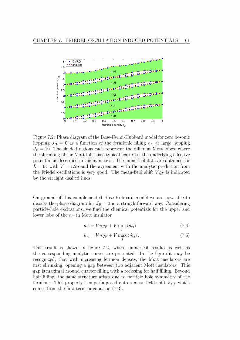
CHAPTER 7. FRIEDEL OSCILLATION-INDUCED POTENTIALS 61
0 0.1 0.2 0.3 0.4 0.5 0.6 0.7 0.8 0.9 10
0.5
1
1.5
2
2.5
3
3.5
4
4.5
5
fermionic density ρF
chem
ical pote
ntial µ
B
n=0
n=1
n=2
n=3
n=4
DMRG
analytic
Figure 7.2: Phase diagram of the Bose-Fermi-Hubbard model for zero bosonichopping JB = 0 as a function of the fermionic filling %F at large hoppingJF = 10. The shaded regions each represent the different Mott lobes, wherethe shrinking of the Mott lobes is a typical feature of the underlying effectivepotential as described in the main text. The numerical data are obtained forL = 64 with V = 1.25 and the agreement with the analytic prediction fromthe Friedel oscillations is very good. The mean-field shift V %F is indicatedby the straight dashed lines.
On ground of this complemented Bose-Hubbard model we are now able todiscuss the phase diagram for JB = 0 in a straightforward way. Consideringparticle-hole excitations, we find the chemical potentials for the upper andlower lobe of the n−th Mott insulator
µ+n = V n%F + V min
j〈mj〉 (7.4)
µ−n = V n%F + V maxj〈mj〉 . (7.5)
This result is shown in figure 7.2, where numerical results as well asthe corresponding analytic curves are presented. In the figure it may berecognized, that with increasing fermion density, the Mott insulators arefirst shrinking, opening a gap between two adjacent Mott insulators. Thisgap is maximal around quarter filling with a reclosing for half filling. Beyondhalf filling, the same structure arises due to particle hole symmetry of thefermions. This property is superimposed onto a mean-field shift V %F whichcomes from the first term in equation (7.3).
62 CHAPTER 7. FRIEDEL OSCILLATION-INDUCED POTENTIALS
Although the explanation for the phase diagram is quite intuitive, it lacksan important feature. As can be seen from figure 7.1, the Friedel oscillationsfor half fermionic filling %F = 1
2are constant over the lattice, resulting in a
closing of the gap between the different Mott lobes. Having a closer look atthe phase diagram for %F = 1
2for large but not infinite values of JF reveals
a completely different behavior which is shown in figure 7.3. Starting withthe local densities of bosons and fermions shown for double half filling, i.e.,%F = %B = 1
2, it can be seen that the fermions, in contrast to the Friedel oscil-
lation prediction, as well as the bosons displays a strict oscillating behavior.This is typical for a so-called charge density wave phase which emerges in thiscase 1. This CDW is a first evidence that the aforementioned back-action ofthe bosons to the fermionic ground state is crucial to understand the physicsin this regime even for larger values of JF . This is even better seen in thenumerically obtained phase diagram in figure 7.3. There it can be seen, thaton the one hand, the Mott lobes do not touch each other and on the otherhand, the CDW phase is incompressible. The extent of the CDW phase,or, more strictly speaking, the metastability region of the CDW phase evenpenetrates that of the Mott insulator, resulting in a thermodynamic instablephase with coexistence of Mott insulator and CDW. With these two indica-tions, pointing to the necessity of a deeper analysis of the system we developa full effective theory of the bosons in the following chapters, explaining themain features of the phase diagram.
1 It may be seen from figure 7.3 that at the center of the system there exists some kindof domain wall. This domain wall is an artefact of the DMRG calculation and only presentfor zero bosonic hopping JB = 0. The Lanczos diagonalization used in DMRG is sometimesproblematic, for instance if the initial state is chosen wrong as happening for the final stepof each sweep. This seems to happen in this case, resulting in some numerical problemswhich are however unimportant in our case since they can be overcome if necessary bymethods shortly discussed later. Here I would like to thank the group of Prof. Eggert foruseful discussions.
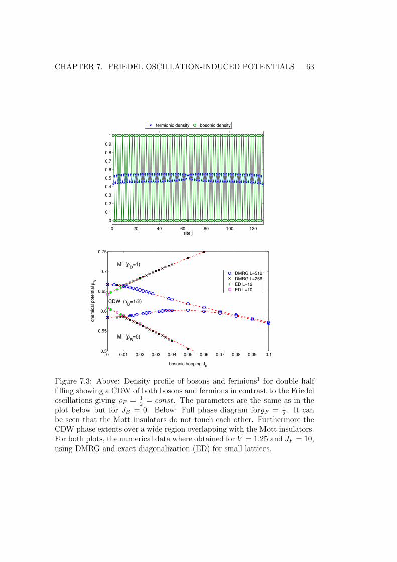
CHAPTER 7. FRIEDEL OSCILLATION-INDUCED POTENTIALS 63
0 20 40 60 80 100 120
0
0.1
0.2
0.3
0.4
0.5
0.6
0.7
0.8
0.9
1
site j
fermionic density bosonic density
0 0.01 0.02 0.03 0.04 0.05 0.06 0.07 0.08 0.09 0.10.5
0.55
0.6
0.65
0.7
0.75
bosonic hopping JB
chem
ical pote
ntial µ
B
CDW (ρB=1/2)
MI (ρB=0)
MI (ρB=1)
DMRG L=512
DMRG L=256
ED L=12
ED L=10
Figure 7.3: Above: Density profile of bosons and fermions1 for double halffilling showing a CDW of both bosons and fermions in contrast to the Friedeloscillations giving %F = 1
2= const. The parameters are the same as in the
plot below but for JB = 0. Below: Full phase diagram for%F = 12. It can
be seen that the Mott insulators do not touch each other. Furthermore theCDW phase extents over a wide region overlapping with the Mott insulators.For both plots, the numerical data where obtained for V = 1.25 and JF = 10,using DMRG and exact diagonalization (ED) for small lattices.

CHAPTER 8
Adiabatic elimination of the fermions
Before we consider the nature of the mentioned back-action, we derive aneffective bosonic model explaining the resulting phase diagram. For generalfermion filling, this is done by first rewriting the Bose-Fermi-Hubbard Hamil-tonian (1.27) such that the notation in the following becomes much simpler.We introduce a bosonic part HB, a fermionic part HF and an interaction partHI, i.e.,
HBFHM = HB + HF + HI (8.1)
with
HB = −JB∑j
(a†j aj+1 + a†j+1aj
)+U
2
∑j
nj (nj − 1) (8.2)
HF = −JF∑j
(c†j cj+1 + c†j+1cj
)+ V
∑j
njmj (8.3)
HI = V∑j
(nj − nj)mj. (8.4)
At this step, we already introduced a bosonic mean-field potential nj in HI
and compensate it by subtracting the term in HF. This term serves lateras the source for the inclusion of the previously mentioned back-action. Forthe moment, this term is kept for simplicity, without a deeper meaning. Theeffective bosonic Hamiltonian is found from an adiabatic elimination, whichis performed in the framework of the scattering matrix
S = T exp
− i~∞∫
−∞
dτHI(τ)
(8.5)
65
66 CHAPTER 8. ADIABATIC ELIMINATION OF THE FERMIONS
of the full system in the interaction picture, i.e.,HI(τ) = e−
i~ (HB+HF)τ HI e
i~ (HB+HF)τ and T being the time ordering
operator. Tracing over the fermionic degrees of freedom yields the bosonicscattering matrix
SBeff = TrF S
=
⟨T exp
− i~ V∑j
∞∫−∞
dτ
(nj(τ)− nj
)mj(τ)
⟩
F
. (8.6)
At this point, we make use of the so-called cumulant expansion [222, 223, 224],which relates the average of an exponential 〈expsX〉X (with respect to astochastic variable X) to the exponential of the averages, i.e., the higherorder cumulants of the stochastic variable
〈expsX〉X = exp
∞∑m=1
sm
m!〈〈Xm〉〉
. (8.7)
Since the cumulants for the fermionic system vanish for orders higher thantwo due to the nature of the fermionic state, the final expression for thebosonic S-matrix is given by
SBeff = T exp
− i~ V∑j
∞∫−∞
dτ(nj(τ)− nj
)〈〈mj(τ)〉〉F (8.8)
− V2
2~2
∑j,l
∞∫−∞
dτ
∞∫−∞
dσ(nj(τ)− nj
)(nl(σ)− nl
)〈〈T mj(τ)ml(σ)〉〉F
.
At this point, the time ordering in the fermionic cumulants is importantas discussed in [225, 226]. So far, no approximations are used, thus theeffective bosonic S-matrix is exact. To derive an effective Hamiltonian forthe bosonic system, an approximation has to be incorporated. As can be seenin equation (8.5), the relation between the Hamiltonian and the scatteringmatrix incorporates a single integral. This form can be reached be applyinga Markov approximation [227, 228], replacing the two-time bosonic density-density operators by equal time operators, i.e.,∞∫
−∞
dτ
∞∫−∞
dσ(nj(τ)− nj
)(nl(σ)− nl
)〈〈T mj(τ)ml(σ)〉〉F
7→∞∫
−∞
dτ(nj(τ)− nj
)(nl(τ)− nl
) ∞∫−∞
dσ 〈〈T mj(τ)ml(σ)〉〉F.
(8.9)
CHAPTER 8. ADIABATIC ELIMINATION OF THE FERMIONS 67
This approximation is valid since the timescale of the fermionic system is1/JF and therefore much shorter than any other timescale in the system. Thisis equivalent to the Born-Oppenheimer approximation in molecular physics,where the heavier (atomic) system is presumed to be static regarding thesolution of the lighter (electronic) system. Using the Markov approximation,we rewrite the bosonic S-matrix as
SBeff = T exp
− i~∞∫
−∞
dτHeffI (τ)
, (8.10)
which defines the effective bosonic interaction Hamiltonian in the interactionpicture
HeffI (τ) = V
∑j
(nj(τ)− nj
)〈〈mj(τ)〉〉F
− iV2
2~∑jl
(nj(τ)− nj
)(nl(τ)− nl
) ∞∫−∞
dσ 〈〈T mj(τ)ml(σ)〉〉F.(8.11)
Since the first order cumulant 〈〈mj(τ)〉〉F is equal to the expectation valueand the second order cumulant1 does only depend on the difference T of thetimes τ and σ and the distance d between the sites j and l as will turn outin the next chapter, the final form of the effective interaction Hamiltonian inthe Schrodinger picture can be written as
HeffI = V
∑j
(nj − nj
)〈mj〉F +
∑j
∞∑d=−∞
gd(%F )(nj − nj
)(nj+d − nj+d
),
(8.12)where the coupling constants gd(%F ) for the induced long range density-density interactions are given by
gd(%F ) = −iV2
2~
∞∫−∞
dT 〈〈T mj(T )mj+d(0)〉〉F. (8.13)
With this result, the whole effect of the fermions on the bosonic subsystemis governed by two terms: (i) the mean-field interaction (1st order) and (ii)the induced density-density interactions (2nd order). In a simple pictorialway, the induced interaction means the scattering of a boson with a fermion
1The definition of the second order cumulant is given by〈〈mj(τ)ml(σ)〉〉 = 〈mj(τ)ml(σ)〉 − 〈mj(τ)〉〈ml(σ)〉.

68 CHAPTER 8. ADIABATIC ELIMINATION OF THE FERMIONS
density−density
fermion−induced
interactionbosons on site i bosons on site i+d
Figure 8.1: Feynman graph representing the fermion induced density-densityinteraction.
on site j with a subsequent second scattering process between the samefermion and another boson at site j + d. A corresponding Feynman diagramfor this process can be found in figure 8.1, illustrating the effective interaction.
Finally, the whole effective Hamiltonian for the bosonic subsystem is givenby equation (8.2) together with equation (8.12):
HeffB = −JB
∑j
(a†j aj+1 + a†j+1aj
)+U
2
∑j
nj (nj − 1) (8.14)
+ V∑j
(nj − nj
)〈mj〉F +
∑j
∞∑d=−∞
gd(%F )(nj − nj
)(nj+d − nj+d
).
As can be seen from equation (8.13), the remaining task in the calculationof the effective Hamiltonian is to calculate the fermionic density-density cor-relator 〈〈T mj(T )mj+d(0)〉〉F using the fermionic Hamiltonian in (8.3). Thiswill be done in the next chapter for the case of free fermions, i.e., nj ≡ 0 forall sites j. This case neglects all possible back-actions of the bosons to thefermions which will be incorporated later by a proper choice of the nj. Theknowledge of the coupling constants at the end allows for a construction ofthe bosonic phase diagram.
CHAPTER 9
Couplings gd(%F ) for free fermions nj ≡ 0
9.1 Calculation of the couplings
a) Determination of the cumulant
Here we calculate the coupling constants from equation (8.13) for the case offree fermions. This is, as mentioned the natural choice, since the fermionichopping amplitude JF is much larger than any other parameter in the systemand hence it can be suspected that the state of the fermions is not affectedby the bosons. Therefore the ground state of the fermions is given by theground state of the fermionic Hamiltonian
HF = −JF∑j
(c†j cj+1 + c†j+1cj
). (9.1)
In momentum space, the solution is straightforward. Applying a Fouriertransform
cj =1√L
L2−1∑
k=−L2
e−2πi kjL fk, (9.2)
the fermionic Hamiltonian transforms into
HF = −2JF∑k
cos(2πk
L) f †k fk. (9.3)
The ground state is the Fermi sphere KF , which means that all momen-tum modes k smaller than the Fermi momentum kF = NF/2 are occupied,
69
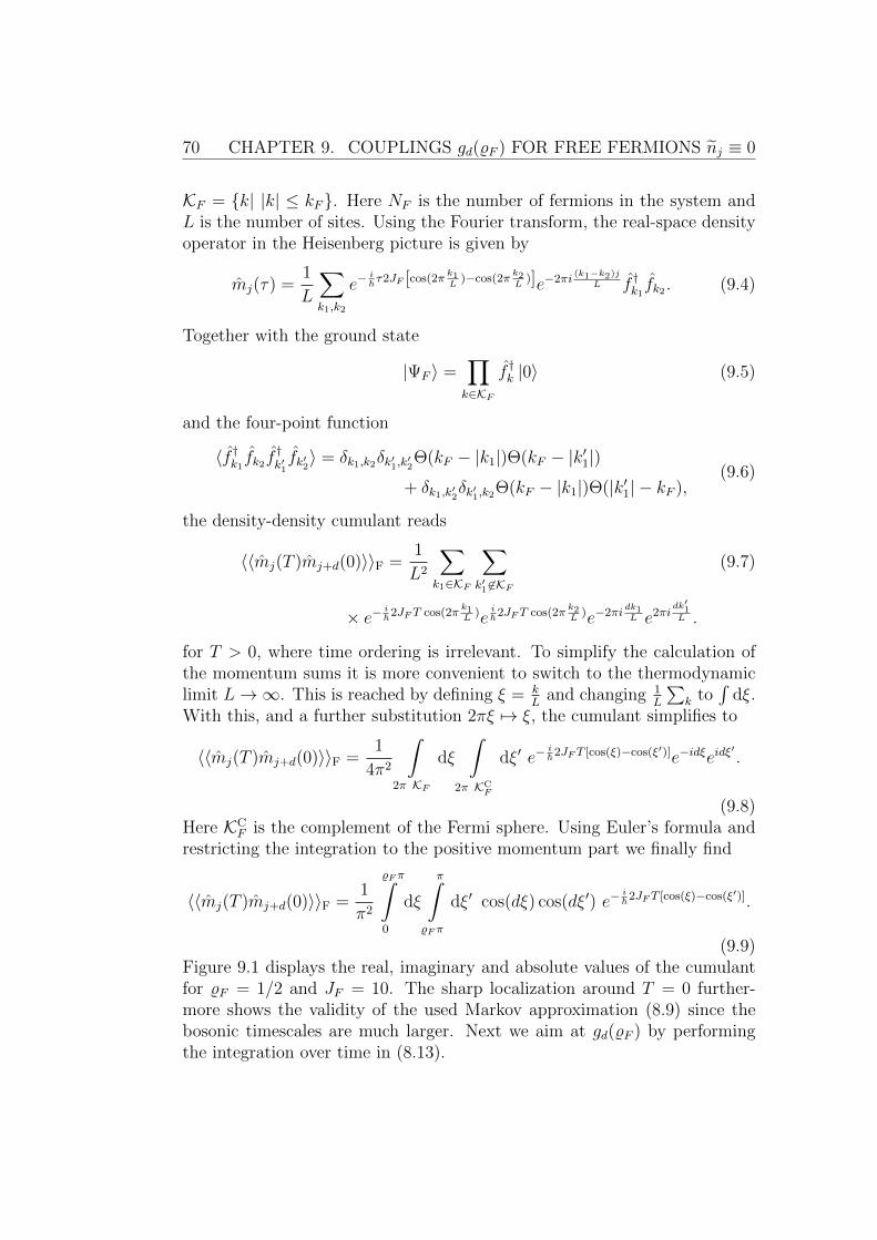
70 CHAPTER 9. COUPLINGS gd(%F ) FOR FREE FERMIONS nj ≡ 0
KF = k| |k| ≤ kF. Here NF is the number of fermions in the system andL is the number of sites. Using the Fourier transform, the real-space densityoperator in the Heisenberg picture is given by
mj(τ) =1
L
∑k1,k2
e−i~ τ2JF [cos(2π
k1L
)−cos(2πk2L
)]e−2πi(k1−k2)j
L f †k1 fk2 . (9.4)
Together with the ground state
|ΨF 〉 =∏k∈KF
f †k |0〉 (9.5)
and the four-point function
〈f †k1 fk2 f†k′1fk′2〉 = δk1,k2δk′1,k′2Θ(kF − |k1|)Θ(kF − |k′1|)
+ δk1,k′2δk′1,k2Θ(kF − |k1|)Θ(|k′1| − kF ),(9.6)
the density-density cumulant reads
〈〈mj(T )mj+d(0)〉〉F =1
L2
∑k1∈KF
∑k′1 6∈KF
(9.7)
× e−i~2JFT cos(2π
k1L
)ei~2JFT cos(2π
k2L
)e−2πidk1L e2πi
dk′1L .
for T > 0, where time ordering is irrelevant. To simplify the calculation ofthe momentum sums it is more convenient to switch to the thermodynamiclimit L→∞. This is reached by defining ξ = k
Land changing 1
L
∑k to
∫dξ.
With this, and a further substitution 2πξ 7→ ξ, the cumulant simplifies to
〈〈mj(T )mj+d(0)〉〉F =1
4π2
∫2π KF
dξ
∫2π KC
F
dξ′ e−i~2JFT [cos(ξ)−cos(ξ′)]e−idξeidξ
′.
(9.8)Here KC
F is the complement of the Fermi sphere. Using Euler’s formula andrestricting the integration to the positive momentum part we finally find
〈〈mj(T )mj+d(0)〉〉F =1
π2
%F π∫0
dξ
π∫%F π
dξ′ cos(dξ) cos(dξ′) e−i~2JFT [cos(ξ)−cos(ξ′)].
(9.9)Figure 9.1 displays the real, imaginary and absolute values of the cumulantfor %F = 1/2 and JF = 10. The sharp localization around T = 0 further-more shows the validity of the used Markov approximation (8.9) since thebosonic timescales are much larger. Next we aim at gd(%F ) by performingthe integration over time in (8.13).

9.1. CALCULATION OF THE COUPLINGS 71
Figure 9.1: Density-density cumulant (9.9) for free fermions splitted in realand imaginary parts as well as the absolute value. %F = 1/2 and JF = 10.The sharp peak around T = 0 shows the validity of the used Markov approx-imation.
b) Calculation of the time integral
The easiest way to perform the time integral over (9.9) is to make use of theRiemann-Lebesgue lemma, which states, that for any L1 function f : R→ C,the Fourier transform of f(t) tends to zero as the frequency tends to infinity[229]
limω→±∞
b∫a
f(t) eiωt dt = 0. (9.10)
When calculating the time integral over equation (9.9), it turns out to besimpler to rewrite the integration together with the time ordering operatoras
∞∫−∞
dT 〈〈T mj(T )mj+d(0)〉〉F = 2 limA→∞
A∫0
dT 〈〈mj(T )mj+d(0)〉〉F. (9.11)
= limA→∞
2
π2
%F π∫0
dξ
π∫%F π
dξ′ cos(dξ) cos(dξ′)
[i~
2JF
e−i~2JFT [cos(ξ)−cos(ξ′)]
cos(ξ)− cos(ξ′)
]A0
.
From the Riemann-Lebesgue lemma, we note that the upper integration limitvanishes for A → ∞. The final result for the coupling constants (8.13) for

72 CHAPTER 9. COUPLINGS gd(%F ) FOR FREE FERMIONS nj ≡ 0
the case of free fermions, i.e. without any back-action of the bosonic systemonto the fermions is thus given by
gd(%F ) = − V 2
2π2JF
%F π∫0
dξ
π∫%F π
dξ′cos(dξ) cos(dξ′)
cos(ξ)− cos(ξ′). (9.12)
This expression for the couplings will be the starting point for our discussionof the phase diagram shown in figure 7.3. As will be seen later, gd(%F )has a singular behavior at %F = 0, 1. For this reason on has to be carefulwith all steps of the calculation here, and we ask the question whether theRiemann-Lebesgue lemma is applicable for this function. The L1-norm ofthe kernel has an upper bound given by the L1-norm of the kernel of g0(%F ).Additionally, the denominator is always positive and therefore
%F π∫0
dξ
π∫%F π
dξ′∣∣∣∣cos(dξ) cos(dξ′)
cos(ξ)− cos(ξ′)
∣∣∣∣ ≤%F π∫0
dξ
π∫%F π
dξ′1
cos(ξ)− cos(ξ′)=π2
4.
(9.13)The last step is proven in the next section. Before we proceed we note that(9.12) shows a particle-hole symmetry gd(%F ) = gd(1 − %F ). This can beshown by substituting ξ → π − ξ and ξ′ → π − ξ′ and interchanging ξ ↔ ξ′
afterwards.
9.2 Couplings in real space
From (9.12), the couplings gd(%F ) can be calculated numerically. We use theprefactor V 2
2π2JFas the energy scale. Only the integral in (9.12) is important
and inherits all vital features. Unfortunately, there does not seem to be ageneral analytic result for it but for d = 0, the integrals can be calculatedanalytically. We find
g0(%F )∣∣∣%F 6=0,1
∼ −%F π∫0
dξ
π∫%F π
dξ′1
cos(ξ)− cos(ξ′)(9.14)
= −2
π∫%F π
dξ′
atanh(
cot(ξ′
2
)tan(ξ2
))sin(ξ)
%F π0
(9.15)
= −π2
4(9.16)
9.2. COUPLINGS IN REAL SPACE 73
0 0.1 0.2 0.3 0.4 0.5 0.6 0.7 0.8 0.9 1−2.5
−2
−1.5
−1
−0.5
0
0.5
1
fermionic density ρF
coup
lings
gd(ρ
F)
[ V
2 /2π2 J F
]
d = 0 d = 1 d = 2 d = 3 d = 5 d = 10
Figure 9.2: Dependence of the coupling strength for various distances d onthe fermionic filling %F . One can obviously see the particle-hole symmetry,reflecting gd(%F ) = gd(1 − %F ) as well as the singular behavior for integerfilling.
for non-integer fermion filling and naturally g0(0) = g0(1) ≡ 0, which showsthat the couplings for zero distance are independent of the density of thefermions. g0 = − V 2
8JFis thus a shift in the bosonic on-site interaction U .
This negative shift is in full agreement with the results from [87, 90, 117],predicting the enhancement of the superfluid phase because of a reductionof the on-site interaction U of the bosons. With our approach, we are ableto go beyond this renormalization of the local U and incorporate furtherinteraction effects.
Figure 9.2 shows the numerical results for the coupling constants as a func-tion of the fermionic filling %F . As stated above, the particle-hole symmetrymanifests itself in the couplings as gd(%F ) = gd(1− %F ). For the case of zeroor unity fermionic filling it should be mentioned, that the coupling constantsare zero in these two cases, whereas the limit lim%F→0,1 gd(%F ) = g0(%F ) isunequal to zero. This effect can be understood when looking at figure 9.3.
Figure 9.3 shows the dependence of the couplings on the distance d forselected densities %F . One can see a periodic modulation of the couplings,with the wavelength of the modulation given by 1/%F (for %F <
12, otherwise
the wavelength is given by 1/(1 − %F )). Therefore, for %F → 0 (or 1)the wavelength diverges and all couplings approach the g0(%F ) value. The

74 CHAPTER 9. COUPLINGS gd(%F ) FOR FREE FERMIONS nj ≡ 0
Figure 9.3: Dependence of the coupling strength for selected densities%F = 0, 1/20, 1/8, 1/4, 1/2 on the distance d. The periods of the oscilla-tions are 1/%F = ∞, 20, 8, 4, 2. For all cases, the signs in the minima arenegative and the maxima positive with a strict alternation from site to sitefor the case of half filling.
behavior of the couplings is typical for induced couplings of the RKKY-type(Rudermann-Kittel-Kasuya-Yosida) [230, 231, 232]. The most interestingcase can be found for %F = 1/2. In this case, the wavelength of 2 leads to astrict alternation in the sign of the couplings from site to site. As a result, theeffective Hamiltonian (8.14) displays repulsive nearest-neighbor, attractivenext-nearest-neighbor, repulsive next-next-nearest-neighbor interaction andso on. See [208] for a similar, numerical study in this case for two dimensions.
From figure 9.4, the reason why a deeper consideration is inevitable in termsof a back-action can be seen. There, the dependence of the coupling constantsis plotted for a larger region of distances for selected %F . More precisely, theabsolute value of the minima, i.e. −gm/%F (%F ) for m ∈ N is shown on adouble logarithmic plot. From the figure it can be seen, that the long-rangedecay of the coupling constants is given by
gd(%F ) ∼ 1
d. (9.17)
Concerning the fitting procedure of the couplings to the numerical datait should be mentioned, that the first few distances were left out and

9.2. COUPLINGS IN REAL SPACE 75
100
101
102
103
10−3
10−2
10−1
100
distance d
−g d(ρ
F)
[ V
2 /2π2 J F
]
d−0.9992
d−0.9995
d−0.9996
d−0.9997
ρF=1/20
ρF=1/8
ρF=1/4
ρF=1/2
Figure 9.4: Absolute value of the couplings g m%F
(%F ) as a function of distance
d for selected densities %F . Points are the numerical integration of the doubleintegral and the solid lines are a linear fit in the double logarithmic plot. Asindicated, the fitting yields a decay of the couplings inverse to the distancefor all densities %F . The slight deviation of the exponent from one can beattributed to the limited set of fitting points.
that the exponent is slightly less than one because of the finite numberof fitting points1. This slow decay of the couplings demands to introducea renormalization procedure, which can be seen from the following argument:
From the numerical data in figure 7.3, we conclude the existence of a CDWphase at double half filling %F = %B = 1
2as also reported in [89, 205] for
slightly different choice of the system parameters. This CDW phase is theresult from the induced interactions. A simple explanation at vanishingbosonic hopping JB can be found by subsequently adding bosons to thesystem starting from zero filling up to the CDW filling %B = 1
2: The
first boson will occupy any site, for instance site 0. When the secondboson is added to the system, the energy will be minimized in site 2 (or−2), since here the density-density interaction is negative, and the overallenergy is reduced. All additional particles will continue occupying all evensites, ending up in the CDW phase at half filling %B = 1/2. But in thisconfiguration, the decay of the couplings with 1
dleads to a divergence of the
total energy in the thermodynamic limit. Since this argument still holdsfor JB > 0, this would result in a CDW of full amplitude ηB = 1 for any
1When increasing the number of fitted data points, the exponents saturate at one.

76 CHAPTER 9. COUPLINGS gd(%F ) FOR FREE FERMIONS nj ≡ 0
0 0.01 0.02 0.03 0.04 0.05 0.06 0.07 0.08 0.09 0.10
0.02
0.04
0.06
0.08
0.1
0.12
0.14
0.16
0.18
0.2
bosonic hopping JB
oscill
ation a
mplit
ude
DMRG ηB (x1/5)
free fermion result
DMRG ηF
a
free fermion ansatz
Figure 9.5: Amplitude of the bosonic CDW as a function of the bosonichopping JB for V = 1.25 and JF = 10. Since the effective theory predicts aCDW for any hopping JB (dashed lines), the necessity of a renormalizationscheme is evident. Additionally the non-zero amplitude of the fermionicCDW is in strong contrast to the underlying ansatz and another indicationof a more involved physics. The numerical data are obtained from DMRGfor lattice of 512 sites and NF = NB = 256.
hopping2. As can be seen in figure 9.5, where the amplitude of the CDWobtained from DMRG simulations is plotted as a function of the bosonichopping, the amplitude of the CDW drops for growing JB, which is incontrast to the results from the coupling constants for free fermions. Weattribute this error to the back-action of the bosons on the fermions which isdisregarded in the effective Hamiltonian by now. Evidence for the existenceof this back-action can also be found from the fermionic CDW amplitudeplotted in figure 9.5. Despite the fact, that the effective theory relies on ahomogeneous fermion distribution (for %F = 1/2) with a proper predictionof a bosonic CDW, the numerics show that the fermions are also found in aCDW phase, with some small, but non-vanishing amplitude ηF . This means,that the inclusion of a possible back-action is essential in the understandingof the phase diagram of the BFHM in the limit of fast fermions. Thesearguments also hold in the case of a fermionic density %F 6= 1
2, with a ground
state which has a boson at every 1%F
-th site3.
2This means an alternation of filled and empty sites.3If the period of the oscillations is commensurable with the lattice. Otherwise, the
situation gets much more complicate.
9.3. COUPLINGS IN MOMENTUM SPACE 77
But before we move onto a scheme including this back-action for %F = 12
we consider the properties of the coupling constants in momentum space.This will provide a valuable tool to judge the performance of the upcomingrenormalization.
9.3 Couplings in momentum space
A different aspect of the nature of the couplings gd(%F ) can be seen from theFourier transform of the couplings:
g%F (k) =∑d
gd(%F )eikd. (9.18)
The analytic form of the couplings (in this case for the free fermion case)shows that the only dependence on the distance d occurs in the numeratorof (9.12). The Fourier transform of the numerator is given by
∞∑d=−∞
cos dξ cos dξ′eikd =π
2
∞∑l=−∞
∑C1,C2=±1
δ(2πl − C1ξ − C2ξ′ − k). (9.19)
as proven in section A.1 in the appendix. The calculation of (9.18) can besimplified by expanding the integration limits to infinity and introducing Θfunctions, since then the evaluation of the δ function is straightforward:
g%F (k) ∼ −%F π∫0
dξ
π∫%F π
dξ′∑
d cos(dξ) cos(dξ′)eikd
cos(ξ)− cos(ξ′)(9.20)
= −π2
%F π∫0
dξ
∞∫−∞
dξ′∑l,C1,C2
Θ(π − ξ′)Θ(ξ′ − π%F )δ(2πl − C1ξ − C2ξ′ − k)
cos(ξ)− cos(ξ′)
Performing the integral over ξ′ finally gives
g%F (k) = − V 2
4πJF
∑l,C1,C2
%F π∫0
dξ × (9.21)
Θ(π − 2πlC2 + C1C2ξ + C2k)Θ(2πlC2 − C1C2ξ − C2k − π%F )
cos(ξ)− cos(C1ξ + k)
as the result for the Fourier transformation of the coupling constants. Thisform already shows the 2π periodicity of g%F (k) due to the sum over l

78 CHAPTER 9. COUPLINGS gd(%F ) FOR FREE FERMIONS nj ≡ 0
100
101
102
−1.3
−1.2
−1.1
−1
−0.9
−0.8
−0.7
−0.6
summation limit s
Σ d=−
ss
g d(0
.5)
[ V
2 /4πJ
F ]
Figure 9.6: Direct summation of the couplings from figure 9.4 for k = 0.On can see the convergence for s → ∞ to −1; this agrees with the limitlimk→0 g 1
2(k).
(times 2π) and the cosine in the denominator. Therefore it is sufficientto restrict the range of k to k ∈ [−π, π]. With this restriction, the rangeof possible l values giving non-zero kernels for the integrals (due to theΘ functions) is strongly limited. For k = 0 it turns out that the integralkernel in (9.21) is not well defined. g 1
2(0) therefore has to be evaluated by
a direct summation of the numerically integrated real space couplings takenfrom figure 9.4 for %F = 1
2. This is shown in figure 9.6, where the Fourier
transform is approximated by a finite sum with increasing limits, yieldingg 1
2(0) = limk→0 g 1
2(k) = − V 2
4πJF.
Figure 9.7 shows the couplings in momentum space as a function of themomentum k and the density %F . From the figure a divergence for k = ±2π%Fmay be seen4. This divergence (van Hove-singularity [233]), also reported forinstance in [117, 213] is directly connected to the earlier discussed divergenceof the energy. For arbitrary fermionic density %F , filling the system withbosons up to a density %B = %F results in a distribution of the bosons wherethe distance between the bosons is given by the wavelength of the couplingconstant as presented in figure 9.3. The total energy of this configurationis related to the Fourier transform of the corresponding wavelength, thusbeing divergent, leading to the peculiarities discussed earlier. With these
4This strictly holds for %F < 12 . For %F > 1
2 , the divergence is situated atk = ±2π(1− %F ) due to the particle-hole symmetry.
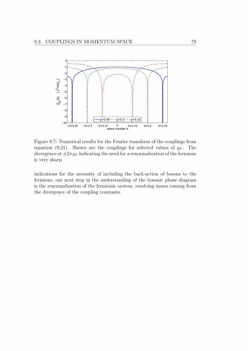
9.3. COUPLINGS IN MOMENTUM SPACE 79
−10
−9
−8
−7
−6
−5
−4
−3
−2
−1
0
wave number k
g ρF(k
)
[ V2 /4
πJF ]
−2π 0.45 −2π 0.3 −2π 0.15 0 2π 0.15 2π 0.3 2π 0.45
~
ρ=0.45 ρ=0.3 ρ=0.15
Figure 9.7: Numerical results for the Fourier transform of the couplings fromequation (9.21). Shown are the couplings for selected values of %F . Thedivergence at±2π%F indicating the need for a renormalization of the fermionsis very sharp.
indications for the necessity of including the back-action of bosons to thefermions, our next step in the understanding of the bosonic phase diagramis the renormalization of the fermionic system, resolving issues coming fromthe divergence of the coupling constants.


CHAPTER 10
Renormalization of the fermionic system and
the effective Hamiltonian
In the present chapter we introduce a renormalization scheme for thecalculation of the fermionic cumulant in (8.13). The back-action of bosonson fermions is incorporated by the introduction of the bosonic mean-fieldamplitude nj in equation (8.3). A natural choice of these amplitudes isapparent from the discussion in the previous chapter. As discussed, theansatz of free fermions drives the bosonic system in a CDW phase with adivergent energy in the thermodynamic limit. This bosonic CDW in turnhas an influence onto the fermionic system. Our approach incorporatesthis influence by a mean-field amplitude nj, following the CDW oscillationsof the bosonic subsystem. The bosonic CDW will act as a backgroundpotential for the fermions. A drawback of our method is the slightly limitedrange of applicability. Due to the complexity of the method, only the case of%F = 1/2 is easily tangibly. Although we can generalize the method to othercommensurate fermionic fillings %F = 1/m with m ∈ N (as done formallyin appendix A.4), we restrict ourselves to half fermionic filling. Finally,the renormalized cumulants are used to calculate and analyze the effectivecoupling constants together with a short discussion of the arising effectivebosonic Hamiltonian.
For the case of a bosonic CDW the mean-field amplitude ansatz1 is given by
nj = %B[1 + ηB(−1)j
]= %B(1− ηB) + 2%BηB δ(sin(π
j
2)), (10.1)
1A similar ansatz is used in [81] to study the influence of the wavelength of the bosonicCDW on the fermionic system.
81

82 CHAPTER 10. RENORMALIZATION AND EFFECTIVE MODEL
where the latter form serves as a simplification in the following calculation.Here we introduced the amplitude of the bosonic CDW ηB as a free pa-rameter. Figure 9.5 shows, that this amplitude drops to zero for increasinghopping JB.
The main task in this chapter is to calculate the fermionic cumulants used inthe effective bosonic Hamiltonian (8.14), i.e., free fermions in an alternatingpotential, given by
HF = −JF∑j
(c†j cj+1 + c†j+1cj
)+ V 2%BηB
∑j
δ(sinπj
2)mj. (10.2)
In this Hamiltonian, a global energy shift V %B(1− ηB)%F from the potentialis left out and a solution can be found straightforwardly, since the Hamilto-nian is only quadratic in the creation and annihilation operators. Althoughthe solution is easy by means of a canonical transformation as presented inappendix A.4 and in [178, 234], the resulting expressions are rather involvedand the quantities needed are hard to express. Here we employ a Green’sfunction approach, extracting all needed quantities for the full calculation ofthe bosonic Hamiltonian for double half filling.
10.1 General framework and initial defini-
tions
Before going into details, we introduce the framework of the calculation. Inorder to calculate the second order cumulant 〈〈mj(T )mj+d(0)〉〉F with respectto the ground state of the fermionic Hamiltonian (10.2) we make use of theGreen’s function technique [220]. The second order cumulant factorizes byuse of Wick’s theorem [220, 235, 236] into a product of the advanced andretarded Green’s functions
〈〈mj(T )mj+d(0)〉〉F =⟨c†j(t+ T )cj+d(t)
⟩⟨cj(t+ T )c†j+d(t)
⟩= G(+)
j,j+d(t+ T, t) G(−)j,j+d(t+ T, t). (10.3)
Here we used T > 0 and the definition of the Green’s functions
G(+)j,j+d(t+ T, t) =< T c†j(t+ T ) cj+d(t) >
G(−)j,j+d(t+ T, t) =< T cj(t+ T ) c†j+d(t) > .
(10.4)
To find a solution of the problem it is more convenient to switch to momentumspace. The Hamiltonian (10.2) can be transformed to momentum space by

10.1. GENERAL FRAMEWORK AND INITIAL DEFINITIONS 83
the Fourier transformation (9.2), which gives
HF = −2JF
L/2−1∑k=−L/2
cos(2πk
L) f †k fk + V ηB%B
L/2−1∑k=−L/2
∑α=±1
f †k+L
2αfk (10.5)
apart from a constant energy shift V ηB%B%F which is neglected. Here itshould be mentioned that the summation over α only includes those termswhich fulfill |k| < L
2. To denote Green’s functions in momentum space
change indices as j → k and j + d→ k′.
Due to the perturbation of the ground state from the potential V , we firstcalculate the Green’s functions (10.4) for the unperturbed system, i.e., theground state of Hamiltonian (10.2) for ηB = 0. This state is the aforemen-tioned Fermi-sphere (9.5). A straightforward calculation gives for the Green’sfunctions
G(0+)k,k′ (t, t′) = Θ(t− t′)Θ(εF − εk)eiεk(t−t′)δk,k′
−Θ(t′ − t)Θ(εk − εF )eiεk(t−t′)δk,k′
G(0−)k,k′ (t, t′) = Θ(t− t′)Θ(εk − εF )eiεk(t′−t)δk,k′
−Θ(t′ − t)Θ(εF − εk)eiεk(t′−t)δk,k′
(10.6)
in the time domain and
G(0±)k,k′ (ω) = ±δk,k′
i√2π
1
εk ∓ ω ⊕ iδ(10.7)
in the frequency domain. Here, the frequency domain is defined by the (time)Fourier transformation
G(0±)k,k′ (ω) =
1√2π
∞∫−∞
dT G(0±)k,k′ (t+ T, t) e−iωT e±δT . (10.8)
The last term in the integral kernel is introduced to assure convergence andwill be properly removed later on. In equation (10.6) we introduced thedispersion relation
εk = −2JF cos(2πk
L) (10.9)
of the free particle and
⊕ =
+ k ∈ KF− k 6∈ KF
(10.10)
84 CHAPTER 10. RENORMALIZATION AND EFFECTIVE MODEL
distinguishes between momentum modes within the Fermi sphere and thoseoutside.
Following the technical details presented in [220], we immediately arrive at aDyson equation for the Green’s function since the induced potential is onlyquadratic in the fermionic operators. In the frequency domain this gives
G(+)k,k′(ω) = G(0+)
k,k′ (ω) +i
~√
2πV ηB%B G(0+)k,k (ω)
∑α=±1
G(+)
k+L2α,k′
(ω) (10.11)
for the advanced Green’s function and the retarded Green’s function is givenby
G(−)k,k′(ω) = G(0−)
k,k′ (ω) +i
~√
2πV ηB%B G(0−)k′,k′ (ω)
∑α=±1
G(−)
k,k′+L2α(ω). (10.12)
These equations allow for an algebraic solution.
10.2 Solution of the Dyson equations
For the solution we only discuss the case of the advanced Green’s function,the situation for the retarded one is exactly the same.
The solution of equation (10.11) can be found by considering
G(+)
k±L2,k′
(ω) = G(0+)
k±L2,k′
(ω) +i
~√
2πV ηB%B G(0+)
k±L2,k±L
2
(ω)G(+)k,k′(ω), (10.13)
which are the contributions in the latter part of equation (10.11). Here it
should be mentioned that the contribution from G(+)k±L,k′(ω) vanishes since
the momentum modes are limited to the first Brillouin zone k ∈ [−L2, L
2]
with k±L 6∈ [−L2, L
2]. Plugging these two Green’s functions into (10.11) and
solving for G(+)k,k′(ω) finally gives the solution of the Green’s functions in terms
of the unperturbed ones:
G(+)k,k′(ω) =
G(0+)k,k′ (ω) + i
~
√2πV ηB%B G(0+)
k,k (ω)[G(0+)
k+L2,k′
(ω) + G(0+)
k−L2,k′
(ω)]
1 +2πV 2η2B%
2B
~2 G(0+)k,k (ω)
[G(0+)
k+L2,k+L
2
(ω) + G(0+)
k−L2,k−L
2
(ω)] .
(10.14)
10.3. GREEN’S FUNCTION IN REAL SPACE 85
From (10.7) we note that G(0±)k,k′ (ω) ∼ δkk′ and therefore only the terms
G(+)k,k (ω), G(+)
k,k±L2
(ω) and G(+)
k±L2,k
(ω) of the full Green’s functions are non-zero.
Applying the same procedure to G(−)k,k′(ω) gives a similar expression. The final
form for the Green’s functions in momentum space and time domain is foundby using the precise form of G(0±)
k,k′ from (10.7) and simplifying the resultingexpressions giving
G(±)k,k (ω) = ± i√
2π
εk ± ω ⊕ iδ(εk ∓ ω ⊕ iδ)(εk ± ω ⊕ iδ) +
V 2η2B%2B
~2
(10.15)
and
G(±)
k,k±L2
(ω) =iV ηB%B√
2π~
(εk ∓ ω ⊕ iδ)(εk ± ω ⊕ iδ) +V 2η2B%
2B
~2
= G(±)
k±L2,k
(ω). (10.16)
Here, again ⊕ distinguishes between momentum modes k within or outsidethe Fermi sphere KF .
This is the main result of this section. It has to be completed by transformingback to the time domain which can be found in appendix A.2. After theFourier transformation, introducing the renormalized dispersion relation
εk =
√ε2k +
V 2η2B%
2B
~2, (10.17)
the Green’s functions in momentum space and time domain are found to read
G(±)k,k (t+ T, t) =
1
2e−iεkT
(1∓ εk
εk
)(10.18)
G(±)
k±L2,k
(t+ T, t) = −V ηB%B2~
1
εke−iεkT . (10.19)
These expressions allow to calculate the density-density correlations for thefermionic Hamiltonian.
10.3 Green’s function in real space
The missing final step, the Fourier transformation from momentum spaceto real space will be performed together with the transition to the ther-modynamic limit. As above, we restrict ourselves on the calculation ofG(+)j,j+d(t+ T, t), since the calculation for G(−)
j,j+d(t+ T, t) is similar.

86 CHAPTER 10. RENORMALIZATION AND EFFECTIVE MODEL
Using the definition
G(+)j,j+d(t+ T, t) =
⟨T c†j(t+ T ) cj+d(t)
⟩(10.20)
of the Green’s functions and the Fourier transformation to momentum space(9.2), the real space Green’s functions are connected to the momentum spaceGreen’s functions by
G(+)j,j+d(t+ T, t) =
1
L
L/2−1∑k1,k2=−L/2
e−2πi(k1−k2)
Lje−2πi
k1LdG(+)
k2,k1(t+ T, t). (10.21)
From the previous discussions we know, that only certain Green’s functionsin momentum space are non-zero. This is incorporated by including
δk1k2 + δk1+L2k2
+ δk1−L2k2
(10.22)
to the summation, picking out the non-zero elements. After performing thesummation over k2, a slight restructuring of the exponentials and an appli-cation of the symmetry of the Green’s functions (10.16), the final result isfound to be2
G(+)j,j+d(t+ T, t) =
1
2L
∑k
e−2πi kLd
[(1− εk
εk)− (−1)j
V ηB%B~
1
εk
]e−iεkT .
(10.23)For a detailed analysis of the Green’s functions, it is more convenient toswitch to the thermodynamic limit. As stated earlier, this is achieved bysubstituting ξ = k
Land changing 1
L
∑k to
∫dξ. Furthermore including the
definition of the free fermion dispersion (10.9) as well as the renormalizeddispersion (10.17) and introducing an amplitude factor
a =V ηB%B2~JF
(10.24)
the real space Green’s functions in time domain can be written as
G(±)jj+d(t+ T, t) =
1
2π
π∫0
dξ cos(dξ) e−iT2JF√
cos2(ξ)+a2
(1± cos(ξ)√
cos2(ξ) + a2
)
− (−1)ja
2π
π∫0
dξ cos(dξ)e−iT2JF
√cos2(ξ)+a2√
cos2(ξ) + a2.
(10.25)
2The retarded form G(−)j,j+d(t+ T, t) is found from a similar analysis.
10.4. EXPECTATORS AND DENSITY-DENSITY CORRELATOR 87
This result is the starting point for the calculation of the density-density cor-relator. Note that the integration in (10.25) cannot be carried out explicitlyfor general arbitrary d.
10.4 Expectation values and the density-
density correlator
The calculation of the Green’s functions does not only allow to calculate ofthe density-density correlator in equation (8.13) but also gives a predictionof the behavior of the fermionic system, as long as the bosonic CDWamplitude ηB is known. Here we first look at the solution of the fermionicproblem itself, i.e., all numerical data shown are calculated for the Hamil-tonian (10.2), i.e., only the fermionic problem with an external potential issimulated; not the full Bose-Fermi-Hubbard Hamiltonian.
a) Local density
The first quantity to study is the fermionic density predicted by the renor-malization procedure. With the result for the Green’s function in equation(10.25) an analytic form for the fermionic density can be found. Using
〈mj〉F = G(+)j,j+0(t+ 0, t) (10.26)
the fermionic density evaluates as
〈mj〉F =1
2π
π∫0
dξ
(1 +
cos(ξ)√cos2(ξ) + a2
)− (−1)j
a
2π
π∫0
dξ1√
cos2(ξ) + a2
=1
2− (−1)j
a
π√
1 + a2K
[1
1 + a2
]. (10.27)
The first important result from the renormalization procedure therefore is
〈mj〉F =1
2
[1− ηaF (−1)j
], (10.28)
where ηaF = 2aπ√
1+a2K[
11+a2
]and K[x] is the complete elliptic integral of
the first kind [237]. This means, the renormalization procedure resultsin the prediction of a fermionic CDW with some amplitude ηaF whichis in agreement with the numerical results from figure 9.5. Figure 10.1
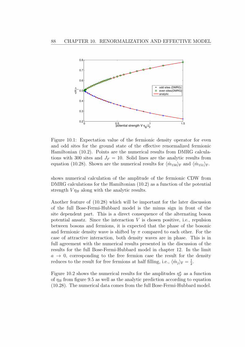
88 CHAPTER 10. RENORMALIZATION AND EFFECTIVE MODEL
0 0.5 1 1.50.2
0.3
0.4
0.5
0.6
0.7
0.8
<m
j>
potential strength V ηB/J
F
odd sites (DMRG)even sites(DMRG)analytic
Figure 10.1: Expectation value of the fermionic density operator for evenand odd sites for the ground state of the effective renormalized fermionicHamiltonian (10.2). Points are the numerical results from DMRG calcula-tions with 300 sites and JF = 10. Solid lines are the analytic results fromequation (10.28). Shown are the numerical results for 〈m150〉F and 〈m151〉F.
shows numerical calculation of the amplitude of the fermionic CDW fromDMRG calculations for the Hamiltonian (10.2) as a function of the potentialstrength V ηB along with the analytic results.
Another feature of (10.28) which will be important for the later discussionof the full Bose-Fermi-Hubbard model is the minus sign in front of thesite dependent part. This is a direct consequence of the alternating bosonpotential ansatz. Since the interaction V is chosen positive, i.e., repulsionbetween bosons and fermions, it is expected that the phase of the bosonicand fermionic density wave is shifted by π compared to each other. For thecase of attractive interaction, both density waves are in phase. This is infull agreement with the numerical results presented in the discussion of theresults for the full Bose-Fermi-Hubbard model in chapter 12. In the limita → 0, corresponding to the free fermion case the result for the densityreduces to the result for free fermions at half filling, i.e., 〈mj〉F = 1
2.
Figure 10.2 shows the numerical results for the amplitudes ηaF as a functionof ηB from figure 9.5 as well as the analytic prediction according to equation(10.28). The numerical data comes from the full Bose-Fermi-Hubbard model.
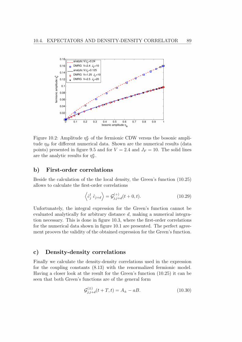
10.4. EXPECTATORS AND DENSITY-DENSITY CORRELATOR 89
0 0.1 0.2 0.3 0.4 0.5 0.6 0.7 0.8 0.9 10
0.02
0.04
0.06
0.08
0.1
0.12
0.14
0.16
0.18
bosonic amplitude ηB
ferm
ionic
am
plit
ude η
Fa
analytic V/JF=0.24
DMRG V=2.4 JF=10
analytic V/JF=0.125
DMRG V=1.25 JF=10
DMRG V=2.5 JF=20
Figure 10.2: Amplitude ηaF of the fermionic CDW versus the bosonic ampli-tude ηB for different numerical data. Shown are the numerical results (datapoints) presented in figure 9.5 and for V = 2.4 and JF = 10. The solid linesare the analytic results for ηaF .
b) First-order correlations
Beside the calculation of the the local density, the Green’s function (10.25)allows to calculate the first-order correlations⟨
c†j cj+d
⟩= G(+)
j,j+d(t+ 0, t). (10.29)
Unfortunately, the integral expression for the Green’s function cannot beevaluated analytically for arbitrary distance d, making a numerical integra-tion necessary. This is done in figure 10.3, where the first-order correlationsfor the numerical data shown in figure 10.1 are presented. The perfect agree-ment prooves the validity of the obtained expression for the Green’s function.
c) Density-density correlations
Finally we calculate the density-density correlations used in the expressionfor the coupling constants (8.13) with the renormalized fermionic model.Having a closer look at the result for the Green’s function (10.25) it can beseen that both Green’s functions are of the general form
G(±)j,j+d(t+ T, t) = A± − aB. (10.30)

90 CHAPTER 10. RENORMALIZATION AND EFFECTIVE MODEL
−0.1
−0.05
0
0.05
VηB/J
F=0.01
−0.1
−0.05
0
0.05
VηB/J
F=0.1
<c
j+ c
j+d>
5 10 15 20 25 30 35 40
−0.1
−0.05
0
0.05
VηB/J
F=0.4
distance d
Analytic DMRG 10−3
10−2
10−1
100
101
−12
−10
−8
−6
−4
−2
0
2
4
6
8x 10
−3
<c
+ j c
j+d>
potential strength VηB/J
F
d=3
d=4
d=5
d=6
d=7
d=8
d=9
d=10
d=11
Figure 10.3: First-order correlations < c†j cj+d > calculated from the fermionmodel (10.2). Solid lines are the theoretical results from a numerical integra-tion of (10.25). The points are the numerical results from the data used infigure 10.1. Left: Distance dependence of the correlations for three differentinteractions V ηB. Right: Dependence of the correlations for a wide range ofinteractions V ηB for selected distances d.
The definitions of A± and B are obvious from equation (10.25). In equation(10.3) we already noted that the density-density cumulant splits up into theproduct of advanced and retarded Green’s function, which may be writtenas
〈〈mj(T )mj+d(0)〉〉F = A+A− − a(A+ + A−) + a2B2. (10.31)
From the definition of the coupling constants (8.13) we can see, that theyare proportional to V 2, since they are a second order correction in theeffective Hamiltonian (8.14). This means, that in order V 2, only the firstterm in (10.31) is relevant.
Following this argument, the renormalized form of the density-density cumu-lant reads
〈〈mj(t+ T )mj+d(t)〉〉 =1
4π2
π∫0
π∫0
dξdξ′ cos(dξ) cos(dξ′)
× e−iT2JF
(√cos2(ξ)+a2+
√cos2(ξ′)+a2
)(10.32)
×
(1 +
cos(ξ)√cos2(ξ) + a2
)(1− cos(ξ′)√
cos2(ξ′) + a2
).
This is the main result from the renormalization procedure. Comparing therenormalized result to that of free fermions (at %F = 1
2) in equation (9.9)

10.5. DISCUSSION OF THE RENORMALIZED COUPLINGS 91
one can see, that the corresponding limit a → 0 gives the same result asequation (9.9). Note, that the last line in (10.32) serves as a cutoff functionwhich constrains the integration limits to the free fermion values in the limita→ 0. In this limit, the free fermion solution is recovered.
10.5 Discussion of the renormalized cou-
plings
As already done in chapter 9, the second order cumulant needs to be inte-grated over time according to equation (8.13) in order to obtain the effectivecoupling constants of the bosonic model. Following the same arguments asin section 9.1b), the time integration may be performed using the Riemann-Lebesgue lemma. The condition, that the integral kernel is a L1 function isfulfilled since the absolute value of the kernel is less than 1
a(1 − a−2) (mod-
ulo some prefactors). This gives an upper bound which reduces in the limita→ 0 to the free fermion which has already been proven to be L1. Thus theRiemann-Lebesgue lemma is applicable, giving for the coupling constants theclosed form
gd(a) = − V 2
8π2JF
π∫0
π∫0
dξdξ′cos(dξ) cos(dξ′)√
cos2(ξ) + a2 +√
cos2(ξ′) + a2
×
(1 +
cos(ξ)√cos2(ξ) + a2
)(1− cos(ξ′)√
cos2(ξ′) + a2
) (10.33)
for the density-density interaction couplings strengths in the effectivebosonic Hamiltonian. Since we restrict ourselves to the case of half filling forthe fermions, the additional index %F is dropped here but the dependence ofthe renormalized couplings on the amplitude factor a is explicitly written.The result is in accordance to the free fermion case since in the limit a→ 0the second line of equation (10.33) gives a factor of 4 together with alimitation of the integration limits to ξ ∈ [0, π
2] and ξ′ ∈ [π
2, π] as in (9.12).
Let us discuss the properties of the renormalized coupling constants. Figure10.4 shows the absolute values for the couplings as a function of the distanced for fixed a = 0.1 compared to the free fermion case a = 0. Whereas thecouplings in the latter case decay as 1/d as discussed in chapter 9, therenormalized couplings decay much faster. This leads to the importantconclusion, that the divergence for k = ±π as shown in figure 9.7 is lifted.
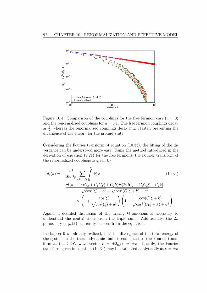
92 CHAPTER 10. RENORMALIZATION AND EFFECTIVE MODEL
100
101
102
10−8
10−6
10−4
10−2
100
distance d
|gd|
[
V2 /2
π2 J F ]
free fermions ( ~ d−1 )renormalized
Figure 10.4: Comparison of the couplings for the free fermion case (a = 0)and the renormalized couplings for a = 0.1. The free fermion couplings decayas 1
d, whereas the renormalized couplings decay much faster, preventing the
divergence of the energy for the ground state.
Considering the Fourier transform of equation (10.33), the lifting of the di-vergence can be understood more easy. Using the method introduced in thederivation of equation (9.21) for the free fermions, the Fourier transform ofthe renormalized couplings is given by
ga(k) = − V 2
16πJF
∑l,C1,C2
π∫0
dξ× (10.34)
Θ(π − 2πlC2 + C1C2ξ + C2k)Θ(2πlC2 − C1C2ξ − C2k)√cos2(ξ) + a2 +
√cos2(C1ξ + k) + a2
×
(1 +
cos(ξ)√cos2(ξ) + a2
)(1− cos(C1ξ + k)√
cos2(C1ξ + k) + a2
).
Again, a detailed discussion of the arising Θ-functions is necessary tounderstand the contributions from the triple sum. Additionally, the 2πperiodicity of ga(k) can easily be seen from the equation.
In chapter 9 we already realized, that the divergence of the total energy ofthe system in the thermodynamic limit is connected to the Fourier trans-form at the CDW wave vector k = ±2%Fπ = ±π. Luckily, the Fouriertransform given in equation (10.34) may be evaluated analytically at k = ±π

10.5. DISCUSSION OF THE RENORMALIZED COUPLINGS 93
−10
−5
−2
−1
−0.5
wave number k
ga(k
) [ V
2/4
πJ
F ]
~
−2π −π 0 π 2π
a= 0.5
a= 0.25
a= 0.1
a= 0.05
a= 0.005
a= 0
Figure 10.5: Fourier transform of the renormalized couplings ga(k) for dif-ferent amplitude factors a. At k = ±π, the divergence for a → 0 is clearlyobservable. For k = 0 the situation is more complicated and a short discus-sion can be found in the main text.
and k = 0. For k = ±π, an analysis of the triple sum in (10.34) showsthat the only contributions to the integral come from the combinations(l, C1, C2) = (±1,±1,±1) and (0,∓1,∓1), (0,−1, 1) as well as (0, 1,−1)for k = 0. In both situations, the integration can be done exactly. This gives
ga(±π) = − V 2
8πJF
1√1 + a2
(2K[
1
1 + a2]− E[
1
1 + a2]
)(10.35)
ga(0) = − V 2
8πJF
1√1 + a2
E[1
1 + a2], (10.36)
with E[x] being the complete elliptic integral of second kind [237].
At this point some remarks about the continuity of the coupling constants inFourier space are necessary. Studies with numerical integration of equation(10.34) show, that the limits lima→0 and limk→0 are not interchangeable. Thisdiscontinuity can be seen in figure 10.5, where the Fourier transform of thecoupling constants is plotted for different amplitude factors a. Fixing themomentum k = 0 and then performing the limit lima→0 gives
lima→0
ga(0) = − V 2
8πJF, (10.37)
94 CHAPTER 10. RENORMALIZATION AND EFFECTIVE MODEL
where on the other hand the limit k → 0 with a = 0 gives
limk→0
g0(k) = − V 2
4πJF. (10.38)
For k → 0 at given a = 0, the kernel in equation (10.34) roughly behaveslike a step function of height 1/k and a support of width k. This resemblesthe properties of Dirac’s δ-function, leading to the discontinuity. In our laterstudies, we will nevertheless use the result for the limit a→ 0 at fixed k = 0since this turns out to be the proper choice.
10.6 The renormalized Hamiltonian
After the initial discussions we are now able to write down the effectivebosonic Hamiltonian for a fixed fermion filling %F = 1/2. It reads
HeffB = −JB
∑j
(a†j aj+1 + a†j+1aj
)+U
2
∑j
nj (nj − 1)
− µ∑j
nj −∆∑j
nj(−1)j +∑j
∑d
gd(a) njnj+d. (10.39)
together with the induced chemical
µ = 2%B ga(0)− V/2 (10.40)
and an induced alternating potential
∆ = 2%BηB ga(π) + V ηaF/2, (10.41)
which are a direct consequence of the fermionic density wave
〈mj〉F =1
2
[1− ηaF (−1)j
](10.42)
with amplitude ηaF/2. The coupling constants of the induced density-densityinteraction are given by (10.33) with the amplitude factor a = V ηB%B
2~JF. For
the Fourier transform, the identities∑d
gd(a) = ga(0) and∑d
(−1)d gd(a) = ga(π), (10.43)
hold.

10.6. THE RENORMALIZED HAMILTONIAN 95
This Hamiltonian (10.39) is the major result in this part. It opens the routefor an understanding of the bosonic phase diagram and allows for a straight-forward perturbative approach. As stated earlier, this Hamiltonian still hasa free parameter a ∼ ηB which has to be chosen self-consistently. This pa-rameter describes the bosonic density wave
nj = %B[1 + ηB(−1)j
](10.44)
with averaged density %B.
The influence of the correction terms in (10.39) to the plain Bose-HubbardHamiltonian are discussed in chapter 12, whereas in the next chapter we firstdiscuss the self-consistent determination of the bosonic amplitude ηB fromthe renormalization scheme.

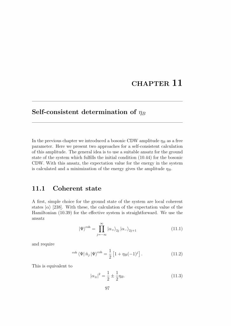
CHAPTER 11
Self-consistent determination of ηB
In the previous chapter we introduced a bosonic CDW amplitude ηB as a freeparameter. Here we present two approaches for a self-consistent calculationof this amplitude. The general idea is to use a suitable ansatz for the groundstate of the system which fulfills the initial condition (10.44) for the bosonicCDW. With this ansatz, the expectation value for the energy in the systemis calculated and a minimization of the energy gives the amplitude ηB.
11.1 Coherent state
A first, simple choice for the ground state of the system are local coherentstates |α〉 [238]. With these, the calculation of the expectation value of theHamiltonian (10.39) for the effective system is straightforward. We use theansatz
|Ψ〉coh =∞∏
j=−∞
|α+〉2j |α−〉2j+1 (11.1)
and require
coh 〈Ψ| nj |Ψ〉coh =1
2
[1 + ηB(−1)j
]. (11.2)
This is equivalent to
|α±|2 =1
2± 1
2ηB. (11.3)
97

98 CHAPTER 11. SELF-CONSISTENT DETERMINATION OF ηB
Assuming real coherent amplitudes α± =√
12± 1
2ηB, the expectation value
for the energy of the effective Hamiltonian is given by
coh 〈Ψ| HeffB |Ψ〉
coh =∑j
[−JB
√1− η2
B +U
8(1 + η2
B) (11.4)
−1
2∆ηB −
1
2µ+
∑d
1
4gd(a)
[1 + (−1)dηB
]+
1
2g0(a)
].
Unfortunately, the coherent state energy functional has a drawback. Sincethe coherent states inherit contributions from all number states, the inter-action part in (11.4) proportional to U dominates. As we are interested inthe double half filling case with approximately no occupation of higher num-ber states n > 1, we may neglect these contributions. Using the results forthe strength ∆ of the induced alternating potential (10.41) and the inducedchemical potential µ (10.40) the energy functional can be written
E [ηB] = −JB√
1− η2B +
1
2g0(a)− 1
4V ηaFηB −
1
4ga(π)η2
B −1
4ga(0). (11.5)
We stress that the amplitude factor a = V ηB4~JF
as well as the fermionic am-plitude ηaF also depend on ηB. The last step is to minimize the energy withrespect to ηB as a function of the parameters of the Bose-Fermi-Hubbardmodel. This needs to be done numerically, since the analytic form of theFourier transformed couplings are too involved. A further simplificationshould be mentioned. Since the numerical evaluation of g0(a) is time con-suming, we use an approximative formula for the region a ∈ [0, 1] which givesa very good agreement to the exact integrals. This is given by
g0(a) ≈ − V 2
8JFπ2
(π2 − 9.92786 a+ 5.41095 a2 − 1.26419 a3
)(11.6)
and the relative error to the numerical integration is less than 10−5 which issufficient for our purpose.
Figure 11.1 compares the self-consistent prediction of the bosonic CDW am-plitude as a function of the bosonic hopping JB to the numerical data fromfigure 9.5 and to data for V = 2.4 and JF = 10. One can see that the co-herent approach gives a qualitatively good agreement for small JB, but thequantitative agreement is rather poor in particular for larger JB because ofthe strongly simplified ansatz used here.
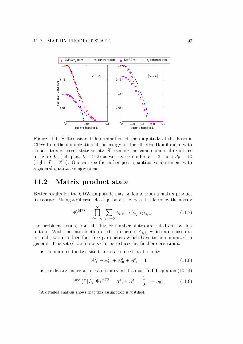
11.2. MATRIX PRODUCT STATE 99
0 0.05 0.10
0.05
0.1
0.15
0.2
bosonic hopping JB
oscill
ation a
mplit
ude
DMRG ηB (x1/5) . η
B coherent state
0 0.05 0.1 0.15 0.20
0.05
0.1
0.15
0.2
bosonic hopping JB
DMRG ηF . η
F coherent state
V=1.25 V=2.4
Figure 11.1: Self-consistent determination of the amplitude of the bosonicCDW from the minimization of the energy for the effective Hamiltonian withrespect to a coherent state ansatz. Shown are the same numerical results asin figure 9.5 (left plot, L = 512) as well as results for V = 2.4 and JF = 10(right, L = 256). One can see the rather poor quantitative agreement witha general qualitative agreement.
11.2 Matrix product state
Better results for the CDW amplitude may be found from a matrix productlike ansatz. Using a different description of the two-site blocks by the ansatz
|Ψ〉MPS =∞∏
j=−∞
1∑i1,i2=0
Ai1i2 |i1〉2j |i2〉2j+1 , (11.7)
the problems arising from the higher number states are ruled out by def-inition. With the introduction of the prefactors Ai1i2 which are chosen tobe real1, we introduce four free parameters which have to be minimized ingeneral. This set of parameters can be reduced by further constraints:
• the norm of the two-site block states needs to be unity
A200 + A2
10 + A201 + A2
11 = 1 (11.8)
• the density expectation value for even sites must fulfill equation (10.44)
MPS 〈Ψ| nj |Ψ〉MPS = A210 + A2
11 =1
2[1 + ηB] , (11.9)
1A detailed analysis shows that this assumption is justified.

100 CHAPTER 11. SELF-CONSISTENT DETERMINATION OF ηB
• the density expectation value for odd sites must fulfill equation (10.44),too
MPS 〈Ψ| nj |Ψ〉MPS = A201 + A2
11 =1
2[1− ηB] . (11.10)
This set of equations allows to reduce the complexity. Introducing three signfunctions α, β, γ = ±1 which are still to be determined, the coefficients havethe form
A01 = αA− A10 = βA+ A11 = γA00 (11.11)
with
A± =
√1
2(1± ηB)− A2
00, (11.12)
which gives a set of parameters which is more easy to handle. The evalu-ation of the expectation value of the energy as a function of the remainingfree parameters is, with exception of the splitting in even and odd sites,straightforward. The result
E[ηB, A00, α, β, γ] =1
2(1−η2
B)[g0(a)−g1(a)
]− V
2ηaFηB−
1
2ga(π)η2
B−1
2ga(0)
+ 2g1(a)A200 − 2γJB
[αβ
γA+A−
(1 + 2A2
00
)+ A2
00
(1− 2A2
00))]
(11.13)
shows, that the choice (α, β, γ) = (1, 1, 1) directly minimizes the energy. Theremaining free parameters are ηB and A00. For these, a numerical mini-mization has to be performed. Beforehand, a further look at the second linereveals, that only there A00 shows up. Analyzing the dependence of the hop-ping contribution on A00 shows, that it is minimal for A00 = 0, which meansthat the state minimizing the energy might have been chosen to be
|Ψ〉MPS =∞∏
j=−∞
(A10 |1〉2j |0〉2j+1 + A01 |0〉2j |1〉2j+1
)(11.14)
from the beginning. This simplification brings the energy functional to itsfinal form, which allows for an easy numerical determination of the minimum:
E[ηB] = −JB√
1− η2B −
V
2ηaFηB −
1
2ga(π)η2
B −1
2ga(0).
+ (1− η2B)[12g0(a)− 1
2g1(a)
].
(11.15)
For the couplings g1(a) again a series expansion in a is used:
g1(a) ≈ V 2
2JFπ2
(0.67492− 0.11149 a− 3.395 a2 + 7.4324 a3 − 5.8053 a4
)(11.16)
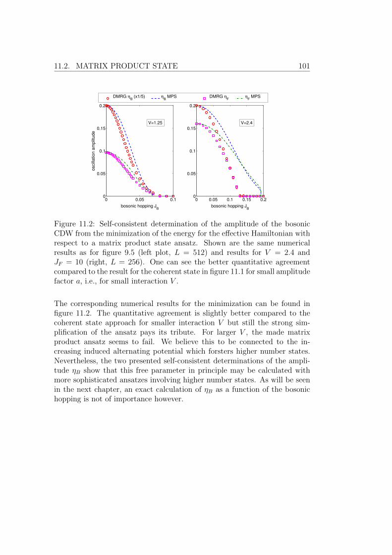
11.2. MATRIX PRODUCT STATE 101
0 0.05 0.10
0.05
0.1
0.15
0.2
bosonic hopping JB
oscill
ation a
mplit
ude
DMRG ηB (x1/5) . η
B MPS
0 0.05 0.1 0.15 0.20
0.05
0.1
0.15
0.2
bosonic hopping JB
DMRG ηF . η
F MPS
V=1.25 V=2.4
Figure 11.2: Self-consistent determination of the amplitude of the bosonicCDW from the minimization of the energy for the effective Hamiltonian withrespect to a matrix product state ansatz. Shown are the same numericalresults as for figure 9.5 (left plot, L = 512) and results for V = 2.4 andJF = 10 (right, L = 256). One can see the better quantitative agreementcompared to the result for the coherent state in figure 11.1 for small amplitudefactor a, i.e., for small interaction V .
The corresponding numerical results for the minimization can be found infigure 11.2. The quantitative agreement is slightly better compared to thecoherent state approach for smaller interaction V but still the strong sim-plification of the ansatz pays its tribute. For larger V , the made matrixproduct ansatz seems to fail. We believe this to be connected to the in-creasing induced alternating potential which forsters higher number states.Nevertheless, the two presented self-consistent determinations of the ampli-tude ηB show that this free parameter in principle may be calculated withmore sophisticated ansatzes involving higher number states. As will be seenin the next chapter, an exact calculation of ηB as a function of the bosonichopping is not of importance however.


CHAPTER 12
Phase diagram of the effective bosonic model
We now use the effective bosonic Hamiltonian
HeffB = −JB
∑j
(a†j aj+1 + a†j+1aj
)+U
2
∑j
nj (nj − 1)
− µ∑j
nj −∆∑j
nj(−1)j +∑j
∑d
gd(a) njnj+d (12.1)
from equation (10.39) to calculate the full phase diagram and compare it tothe numerical results from figure 7.3. As a reminder, the potentials µ and ∆are given by
µ = 2%B ga(0)− V/2 ∆ = 2%BηB ga(π) + V ηaF/2. (12.2)
The calculation itself is done in the same way as in part I for the Bose-Fermi-Hubbard model with immobile fermions. The calculation of the incompress-ible phases is accomplished by calculating the energy of the relevant groundstate within the incompressible phase as well as with one particle added or re-moved. From these energies, the chemical potentials are deduced. In the firstsection we will restrict ourselves to the zero-hopping limit JB = 0 whereasin the second section we will employ a full degenerate perturbation theoryin order to calculate the small JB behavior of the phases. Concerning thebosonic amplitude ηB it should be mentioned, that both, in the zero hoppinglimit1 as well as in the small hopping region, ηB = 1. In the latter situationthis is the case because the perturbation theory starts at JB = 0 and allenergies and quantities are to be calculated for this case.
1Here the amplitude naturally equals one.
103

104 CHAPTER 12. EFFECTIVE BOSONIC PHASE DIAGRAM
12.1 Zero-hopping phase diagram
The calculation of the chemical potentials for JB = 0 is straightforward.Here we only summarize the results; the calculation of some exemplaryenergies can be found in appendix A.3. We however make some remarks onthe nature of the ground state and the notation used.
In the following we deal with states containing a fixed number of particles,or, to be more precise, having a fixed density. For the classification of thesestates we use a short graphical notation. For instance the ground state ofthe CDW (with full amplitude) is written as∣∣ΨN=L/2
⟩ ∧= • • ‖ • ‖ • •, (12.3)
where an open circle ”” means no boson and a filled circle ”•” means thepresence of a boson. This corresponds to the ansatz (10.44) made for thebosonic CDW. With the ansatz (10.44), we explicitly break the symmetryof the system, demanding the bosons to be situated at even sites. Thisis marked by the introduction of the vertical lines and the boson at site j = 0.
For the calculation of the energies we make a suitable ansatz for the soughtstates and replace the number operators in the Hamiltonian (12.1) by realnumbers according to the particular state. This is done for the three incom-pressible phases presented in figure 7.3 which are at %B = 0, 1
2, 1. For each,
an exemplary calculation can be found in the appendix A.3. The ansatz in(10.44) together with the bosonic density allows not only for the descriptionof the CDW at half filling with amplitude one (%B = 1
2, ηB = 1), but also for
a possible CDW at unity filling with amplitude two (%B = 1, ηB = 1) and apure Mott insulator (%B = 1, ηB = 0).
a) CDW phase %B = 12
The relevant states for the calculation of the chemical potentials for theupper and the lower boundary of the incompressible CDW region are givenfor particle numbers N = L/2 − 1, L/2 and L/2 + 1. For the first two, theground state can be found easily. Only the case N = L/2 + 1 is a bit morecomplicated.
The energy of the ground state at double half filling, given by the bo-son distribution shown in (12.3) can be calculated by plugging the density

12.1. ZERO-HOPPING PHASE DIAGRAM 105
nj = nj = 12
[1 + (−1)j] into the expectation value of the Hamiltonian. Thisgives
E(L/2) = E[• • ‖ • ‖ • •] = −1
2µL− 1
2∆L+
1
4L [ga(0) + ga(π)] (12.4)
which naturally depends on the length of the system. But since we are onlyinterested in the chemical potentials
µ±12
= ±(E(L/2± 1)− E(L/2)
), (12.5)
this dependence drops out.
For the calculation of the lower boundary we consider the case of a missingparticle. The position, at which the particle is removed, is unimportant,since the system is translationally invariant with a period two. Therefore theenergy for this situation is given by
E(L/2− 1) = E[• • ‖ ‖ • •] (12.6)
= E[• • ‖ • ‖ • •] + µ+ ∆− ga(0)− ga(π) + g0(a)
and the chemical potential for the lower bound results in
µ−12
=V
2− V
2ηaF − g0(a). (12.7)
As mentioned earlier, we have to choose the amplitude factora = V ηB%B
2~JF= V ηB
4~JFfor ηB = 1 and %B = 1
2.
The calculation for the upper lobe is a bit more involved, because thesuitable ground state is not obvious. Here, two possible situations occur:
• • ‖ • ‖ • • • ⇒ nj = nj + δj,1, (12.8)
• • ‖ •• ‖ • • ⇒ nj = nj + δj,0. (12.9)
As shown in appendix A.3, the energies for these two configurations are givenby
E[• • ‖ • ‖ • • •] = E[• • ‖ • ‖ • •] (12.10)
− µ+ ∆ + ga(0)− ga(π) + g0(a)
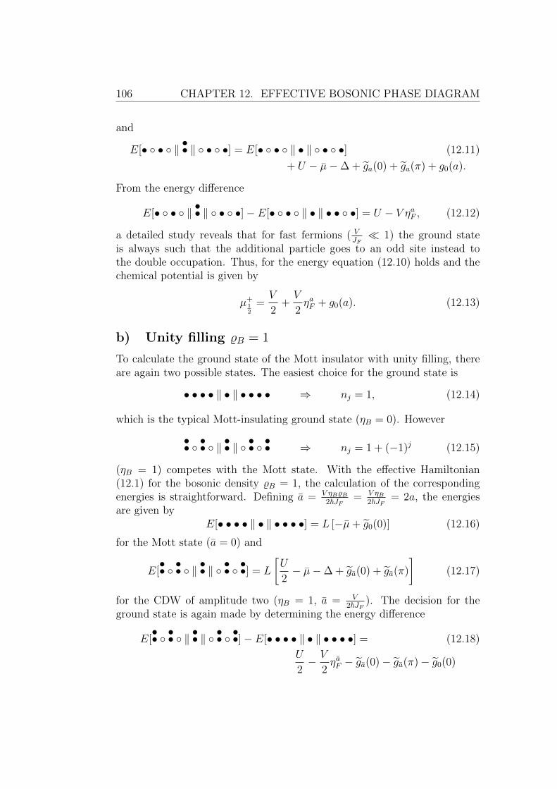
106 CHAPTER 12. EFFECTIVE BOSONIC PHASE DIAGRAM
and
E[• • ‖ •• ‖ • •] = E[• • ‖ • ‖ • •] (12.11)
+ U − µ−∆ + ga(0) + ga(π) + g0(a).
From the energy difference
E[• • ‖ •• ‖ • •]− E[• • ‖ • ‖ • • •] = U − V ηaF , (12.12)
a detailed study reveals that for fast fermions ( VJF 1) the ground state
is always such that the additional particle goes to an odd site instead tothe double occupation. Thus, for the energy equation (12.10) holds and thechemical potential is given by
µ+12
=V
2+V
2ηaF + g0(a). (12.13)
b) Unity filling %B = 1
To calculate the ground state of the Mott insulator with unity filling, thereare again two possible states. The easiest choice for the ground state is
• • • • ‖ • ‖ • • • • ⇒ nj = 1, (12.14)
which is the typical Mott-insulating ground state (ηB = 0). However
•• •• ‖ •• ‖ •• •• ⇒ nj = 1 + (−1)j (12.15)
(ηB = 1) competes with the Mott state. With the effective Hamiltonian(12.1) for the bosonic density %B = 1, the calculation of the correspondingenergies is straightforward. Defining a = V ηB%B
2~JF= V ηB
2~JF= 2a, the energies
are given byE[• • • • ‖ • ‖ • • • •] = L [−µ+ g0(0)] (12.16)
for the Mott state (a = 0) and
E[•• •• ‖ •• ‖ •• ••] = L
[U
2− µ−∆ + ga(0) + ga(π)
](12.17)
for the CDW of amplitude two (ηB = 1, a = V2~JF
). The decision for theground state is again made by determining the energy difference
E[•• •• ‖ •• ‖ •• ••]− E[• • • • ‖ • ‖ • • • •] = (12.18)
U
2− V
2ηaF − ga(0)− ga(π)− g0(0)
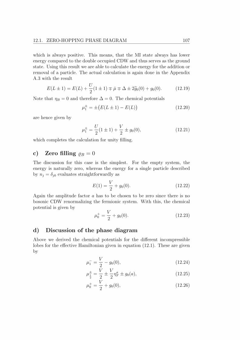
12.1. ZERO-HOPPING PHASE DIAGRAM 107
which is always positive. This means, that the MI state always has lowerenergy compared to the double occupied CDW and thus serves as the groundstate. Using this result we are able to calculate the energy for the addition orremoval of a particle. The actual calculation is again done in the AppendixA.3 with the result
E(L± 1) = E(L) +U
2(1± 1)∓ µ∓∆± 2g0(0) + g0(0). (12.19)
Note that ηB = 0 and therefore ∆ = 0. The chemical potentials
µ±1 = ±(E(L± 1)− E(L)
)(12.20)
are hence given by
µ±1 =U
2(1± 1) +
V
2± g0(0), (12.21)
which completes the calculation for unity filling.
c) Zero filling %B = 0
The discussion for this case is the simplest. For the empty system, theenergy is naturally zero, whereas the energy for a single particle describedby nj = δj0 evaluates straightforwardly as
E(1) =V
2+ g0(0). (12.22)
Again the amplitude factor a has to be chosen to be zero since there is nobosonic CDW renormalizing the fermionic system. With this, the chemicalpotential is given by
µ+0 =
V
2+ g0(0). (12.23)
d) Discussion of the phase diagram
Above we derived the chemical potentials for the different incompressiblelobes for the effective Hamiltonian given in equation (12.1). These are givenby
µ−1 =V
2− g0(0), (12.24)
µ±12
=V
2± V
2ηaF ± g0(a), (12.25)
µ+0 =
V
2+ g0(0), (12.26)
108 CHAPTER 12. EFFECTIVE BOSONIC PHASE DIAGRAM
0 0.5 1 1.5 2 2.5 3−0.2
−0.15
−0.1
−0.05
0
0.05
0.1
0.15
0.2
interaction V
chem
ical pote
ntial −
V/2
µ−
1/2µ
+
1/2 analytic
µ0
+µ
1
−
analytic
CDW+MI
CDW+MI
CDW
MI
MI
Figure 12.1: Phase diagram of the effective bosonic Hamiltonian for vanishingbosonic hopping JB = 0. Data points are the numerical and the solid linesare the analytic results. The shaded region depicts the region where theextent of the CDW phase overlaps with the Mott insulators giving a phaseof coexistence of these two.
which together with the results for the couplings gd(a) and the fermionicCDW amplitude ηaF from chapters 9 and 10 allow to construct the phasediagram at zero bosonic hopping. This is shown in figure 12.1, where thechemical potentials are displayed as a function of the interaction V for afixed fermionic hopping JF . Note that the chemical potentials µ±1
2
for the
CDW lobe enclose the chemical potentials µ+0 and µ−1 for the Mott lobes.
The shaded region in figure 12.1 depicts exactly this region. This behavioris uncommon, since it indicates a negative compressibility
κ =∂〈N〉∂µB
< 0. (12.27)
Starting with the case of half filling, adding particles will lead to a formationof a spatially connected region of unity filling (for sufficient small hopping).This can be seen as follows: the first additional particle can go to any emptysite of the CDW. The next particle will occupy a previously unoccupied siteclosest to the first additional particle since this requires the lowest energydue to the attractive long-range interaction for even distances. A similarargument can be made for the third particle and so on. Thus, within thisregion of the (µB, JB)-phase diagram, there is a phase separation between aMott insulator and a CDW. These kind of coexistence phases are not new

12.2. 2ND ORDER STRONG-COUPLING THEORY 109
(see e.g. [200, 205, 206, 208] for a variety of different coexistence phases),but the coexistence of a Mott insulator and a CDW phase has to ourknowledge not been reported before.
The data points are obtained from numerical results, where the Mott insula-tors are calculated using a finite size extrapolated exact diagonalization andthe numerical results for the CDW are resulting from DMRG calculationswhere the boson distribution is fixed, acting as a potential to the fermions.This procedure is necessary here, since the full DMRG for this system hassevere problems in obtaining the proper ground state. The reason for this ison the one hand the sensitivity of the system to the boundary in the openboundary DMRG and on the other hand the problem of seeking the groundstate within the energy manifold with many close-lying meta-stable states.This complicates the numerical calculation enormously. A detailed discussionof these issues can be found in the last section of this chapter.
12.2 2nd order strong-coupling theory
After the discussion of the phase diagram for zero hopping JB = 0, showingthe existence of phases of coexistence between Mott insulator and CDW,we aim in this section at a perturbation theory in the hopping amplitudeJB to generate the full phase diagram in the (µ − JB) plane. Since themethodology of the perturbation theory will also be used in part IV, werestrict ourselves on the presentation of the basic ideas here. The details ofthe calculation may be found in part IV.
In order to perform a second order perturbation theory we need the energyof the involved ground states as a function of the bosonic hopping JB.For the states corresponding to the filling of the incompressible phasesthis is quite easy. In this case, the ground state is non-degenerate andsimple perturbation theory is sufficient. When adding or removing asingle particle, the ground state is degenerate, since all possible positionsof the extra or less particle are allowed2. The resulting ground-statemanifold consisting of states |Ψ〉j3 requires a non-degenerate perturba-tion theory, where several equivalent formulations are available as forinstance used in [97] for the pure and disordered Bose Hubbard model.
2The removing is of course only allowed if a particle exists in this site for the groundstate.
3The index j labels the different states within the manifold. For the Mott insulators,the additional particle is located at the site j, for the CDW phase at site 2j + 1.
110 CHAPTER 12. EFFECTIVE BOSONIC PHASE DIAGRAM
Here we use Kato’s expansion [159, 170, 239, 240], which relies on thecalculation of an effective Hamiltonian (in arbitrary order) within thedegenerate subspace. The last step is to solve this effective Hamiltonianand obtain the ground-state energy as a function of the perturbationparameter. In part I we already made use of this method in the derivationof the effective model for the composite particles according to [121, 158, 160].
Before we discuss the analytic results, we at least outline the used method.Up to second order, Kato’s expansion is given by
Heff = E0 + PH1P + PH1Q1
E0 − H0
QH1P , (12.28)
where P is the projector onto the degenerate subspace, Q = 1 − P theorthogonal projector and E0 is the zero order energy of the manifold. Here,the Hamiltonian is written in the form
H = H0 + H1, (12.29)
where H1 is the perturbation, i.e., the hopping in our case. The calculation ofthe effective Hamiltonian is now straightforward. The first step is to take anystate |Ψ〉j from the degenerate subspace and apply a single hopping operationto this state. Those parts which are still within the subspace (found by theprojector P) give a first-order contribution and connect the state |Ψ〉j tothe state |Ψ〉m; for those outside the manifold (surviving the projector Q)the second order term holds. For this term, the energy resolvent for theintermediate state is evaluated and the final hopping brings the state backto the initial state |Ψ〉j, or, if possible, to another state |Ψ〉k within the
manifold. Thus the action of the effective Hamiltonian Heff on the state |Ψ〉jhas the form
Heff |Ψ〉j = E0(|Ψ〉j)+J1
[|Ψ〉j−1 + |Ψ〉j+1
]+J2
[|Ψ〉j−2 + |Ψ〉j+2
]+W |Ψ〉j .
(12.30)The special form of the perturbation in our case is already taken into account(see part IV for a more general form of the perturbation). This (maximally)tridiagonal matrix representation of the effective Hamiltonian can be solvedby a Fourier transform, which gives the energy
E = E0 + 2J1 cos(2πk
L) + 2J2 cos(4π
k
L) +W, (12.31)
where the k mode has to be chosen such that the energy is minimal. Inthis system this is typically the case for k = 0 since both J1 ∼ JB and
12.2. 2ND ORDER STRONG-COUPLING THEORY 111
J2 ∼J2B
E0−〈H0〉are negative (the energy resolvent for the intermediate state is
always negative). This procedure has to be done for all involved ground stateswith the proper number of particles, i.e., N = 1, L/2−1, L/2, L/2+1, L−1, L.The calculation is lengthy and does not provide a deeper insight. Neverthelesswe give a graphical representation of the intermediate states as well as thefinal states in figure 12.2. This gives deeper insight into the possible processesin second order, where inversion symmetric processes are not shown. Acrucial point comes from the nature of the effective bosonic Hamiltonianin (12.1). Since the density-density interaction is long ranged, the energydenominator depends on the distance of the particle performing the firsthopping process from the reference site where the additional particle (hole)is situated. This needs to be taken into account for the calculation of thechemical potentials.
As a result, we will here only give the chemical potentials for the consideredlobes. These are given by
µ+0 =
V
2+ g0(0)− 2JB (12.32)
µ−12
=V
2− V
2ηaF − g0(a) + 2J2
B
(1
V ηaF + 2g0(a)− 4g1(a) + 2g2(a)
− 1
V ηaF + 4g0(a)− 4g1(a)−∑m even
[1
V ηaF + 2g0(a)− 2g1(a)(12.33)
− 1
V ηaF + 2g0(a)− 2g1(a) + 2gm(a)− 2gm+1(a)
])
µ+12
=V
2+V
2ηaF + g0(a)− 2J2
B
(4
U + V ηaF + 4g0(a)− 4g1(a)
− 1
V ηaF + 4g0(a)− 4g1(a)+
1
V ηaF + 2g0(a)− 4g1(a) + 2g2(a)
+2
U − V ηaF−∑m even
[1
V ηaF + 2g0(a)− 2g1(a)(12.34)
− 1
V ηaF + 2g0(a)− 2g1(a) + 2gm(a)− 2gm−1(a)
])
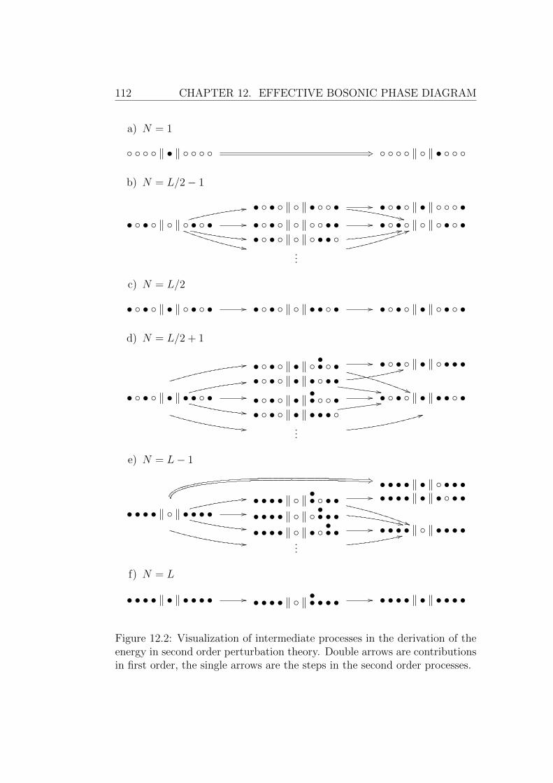
112 CHAPTER 12. EFFECTIVE BOSONIC PHASE DIAGRAM
a) N = 1
‖ • ‖ +3 ‖ ‖ •
b) N = L/2− 1
• • ‖ ‖ • •++
// • • ‖ • ‖ •• • ‖ ‖ • •
11
,,..
// • • ‖ ‖ • • // • • ‖ ‖ • •• • ‖ ‖ • •
33
...
55
c) N = L/2
• • ‖ • ‖ • • // • • ‖ ‖ • • • // • • ‖ • ‖ • •
d) N = L/2 + 1
• • ‖ • ‖ •• • //
((
• • ‖ • ‖ • • •11
• • ‖ • ‖ • • •33
--[[[[[[[[[[
• • ‖ • ‖ • • •--
11
// • • ‖ • ‖ •• • // • • ‖ • ‖ • • •
..• • ‖ • ‖ • • •
11cccccccccc
...
44
e) N = L− 1
• • • • ‖ • ‖ • • •*2
• • • • ‖ ‖ •• • • //
))
• • • • ‖ • ‖ • • •• • • • ‖ ‖ • • • • //
..
00
• • • • ‖ ‖ •• • •++
..• • • • ‖ ‖ • •• • // • • • • ‖ ‖ • • • •
...
33
f) N = L
• • • • ‖ • ‖ • • • • // • • • • ‖ ‖ •• • • • // • • • • ‖ • ‖ • • • •
Figure 12.2: Visualization of intermediate processes in the derivation of theenergy in second order perturbation theory. Double arrows are contributionsin first order, the single arrows are the steps in the second order processes.

12.2. 2ND ORDER STRONG-COUPLING THEORY 113
0 0.01 0.02 0.03 0.04 0.05 0.06 0.07 0.08 0.09 0.10.5
0.55
0.6
0.65
0.7
0.75
bosonic hopping JB
chem
ical pote
ntial µ
B
CDW (ρB=1/2)
MI (ρB=0)
MI (ρB=1)
DMRG L=512
DMRG L=256
ED L=12
ED L=10
2nd order
Figure 12.3: Analytic results for the phase diagram together with the numer-ical results from figure 7.3. The agreement between the analytics and thenumerics is quite reasonable with the natural deterioration for larger hop-ping JB due to the perturbative treatment. Though the critical point for thevanishing of the CDW lobe is underestimated, the general agreement is quitesatisfactory.
µ−1 =V
2− g0(0) + 2JB − 4J2
B
(1
U+
1
U + 4g0(0)− 4g1(0)(12.35)
− 1
U + 2g0(0)− 4g1(0) + 2g2(0)+∑m
[1
U + 2g0(0)− 2g1(0)
− 1
U + 2g0(0)− 2g1(0) + 2gm+1(0)− 2gm(0)
])
A major problem is the aforementioned dependence of the results on allcoupling strengths gd(a), which need to be calculated up to a large distance.For the analytic results used in figure 12.3 it turns out, that d ≈ 100 issufficient to gain convergence. A possible series expansion of the summandsfor the CDW case does not work out because all parts in the denominator areof the same order. Using (12.32)-(12.35) and directly plugging in numbersfor the data from figure 7.3 allows for the determination of the behavior ofthe incompressible lobes. This gives
µ+0 = 0.605469− 2JB, (12.36)
µ−12
= 0.583612 + 33.076J2B, (12.37)

114 CHAPTER 12. EFFECTIVE BOSONIC PHASE DIAGRAM
µ+12
= 0.666388− 45.4392J2B, (12.38)
µ−1 = 0.644531 + 2JB − 4.12927J2B (12.39)
for the chemical potentials which are shown together with the numerical re-sults in figure 12.3. From the figure it may be seen, that the overall agreementis quite reasonable, whereas the quantitative prediction, especially of the tipof the CDW lobe, is not that satisfying.
12.3 Boundary effects in an effective model
with long-range interactions
As already mentioned at several places, boundary effects play an importantrole in this system. The long-range character of the fermion mediatedinteractions leads to a substantial modification of the system dynamicseven for relatively large systems4. This can directly be seen for the case ofthe CDW phase, where we first discuss the zero hopping case. Assumingthe bosons (within the effective Hamiltonian) to be in CDW phase, i.e.,half filling, and adding an additional particle to the system, this particleoccupies an odd site (i.e., a previously unoccupied site). If the particlewould choose the site close to the center of the system, the energy to bepaid is
∑L/4d=−L/4 g2d+1, whereas a particle at the border will only pay the
energy∑L/2
d=0 g2d+1. Remember that all the couplings at odd distances arepositive. Because of the decay of the couplings with distance, the firstsum is much larger then the latter one, resulting in the particle to pin tothe border. Now, with a second additional particle, the same argumentholds and the particle also pins to the border. Because of the attractivenext-nearest-neighbor interaction, this takes place at a distance of two fromthe first additional particle as was the case in the infinite system discussedbefore. This gives a ground state, where a Mott plateau is continuouslybuilding up from the boundary, reaching further and further into the CDWphase when adding more particles. As long as the hopping is small comparedto the energy difference between the state with a particle pinned close to theborder and the state with the additional particle at the center, the reductionof the interaction energy due to the pinning to the boundary dominates theincrease of the kinetic energy. When removing a particle from the system,i.e., going below half filling, the same arguments apply.
4Also the convergence of the DMRG seems to be affected by the boundaries
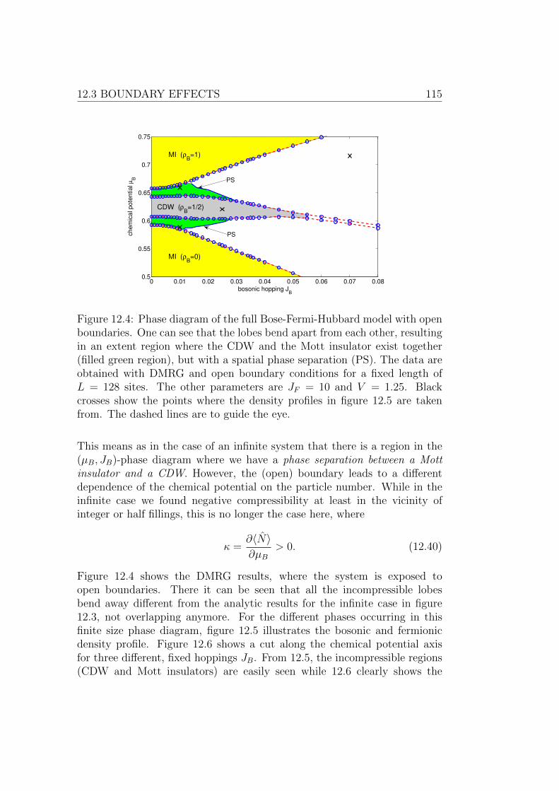
12.3 BOUNDARY EFFECTS 115
0 0.01 0.02 0.03 0.04 0.05 0.06 0.07 0.080.5
0.55
0.6
0.65
0.7
0.75
bosonic hopping JB
chem
ical pote
ntial µ
B
CDW (ρB=1/2)
MI (ρB=0)
MI (ρB=1)
PS
PS
Figure 12.4: Phase diagram of the full Bose-Fermi-Hubbard model with openboundaries. One can see that the lobes bend apart from each other, resultingin an extent region where the CDW and the Mott insulator exist together(filled green region), but with a spatial phase separation (PS). The data areobtained with DMRG and open boundary conditions for a fixed length ofL = 128 sites. The other parameters are JF = 10 and V = 1.25. Blackcrosses show the points where the density profiles in figure 12.5 are takenfrom. The dashed lines are to guide the eye.
This means as in the case of an infinite system that there is a region in the(µB, JB)-phase diagram where we have a phase separation between a Mottinsulator and a CDW. However, the (open) boundary leads to a differentdependence of the chemical potential on the particle number. While in theinfinite case we found negative compressibility at least in the vicinity ofinteger or half fillings, this is no longer the case here, where
κ =∂〈N〉∂µB
> 0. (12.40)
Figure 12.4 shows the DMRG results, where the system is exposed toopen boundaries. There it can be seen that all the incompressible lobesbend away different from the analytic results for the infinite case in figure12.3, not overlapping anymore. For the different phases occurring in thisfinite size phase diagram, figure 12.5 illustrates the bosonic and fermionicdensity profile. Figure 12.6 shows a cut along the chemical potential axisfor three different, fixed hoppings JB. From 12.5, the incompressible regions(CDW and Mott insulators) are easily seen while 12.6 clearly shows the
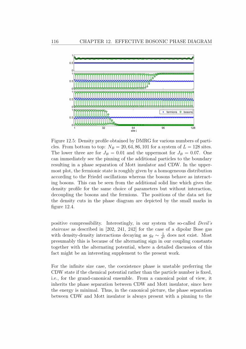
116 CHAPTER 12. EFFECTIVE BOSONIC PHASE DIAGRAM
1 32 64 96 1280
0.5
1
site j
fermions bosons
0
0.5
10
0.5
10
0.5
1
Figure 12.5: Density profile obtained by DMRG for various numbers of parti-cles. From bottom to top: NB = 20, 64, 86, 101 for a system of L = 128 sites.The lower three are for JB = 0.01 and the uppermost for JB = 0.07. Onecan immediately see the pinning of the additional particles to the boundaryresulting in a phase separation of Mott insulator and CDW. In the upper-most plot, the fermionic state is roughly given by a homogeneous distributionaccording to the Friedel oscillations whereas the bosons behave as interact-ing bosons. This can be seen from the additional solid line which gives thedensity profile for the same choice of parameters but without interaction,decoupling the bosons and the fermions. The positions of the data set forthe density cuts in the phase diagram are depicted by the small marks infigure 12.4.
positive compressibility. Interestingly, in our system the so-called Devil’sstaircase as described in [202, 241, 242] for the case of a dipolar Bose gaswith density-density interactions decaying as gd ∼ 1
d3does not exist. Most
presumably this is because of the alternating sign in our coupling constantstogether with the alternating potential, where a detailed discussion of thisfact might be an interesting supplement to the present work.
For the infinite size case, the coexistence phase is unstable preferring theCDW state if the chemical potential rather than the particle number is fixed,i.e., for the grand-canonical ensemble. From a canonical point of view, itinherits the phase separation between CDW and Mott insulator, since herethe energy is minimal. Thus, in the canonical picture, the phase separationbetween CDW and Mott insulator is always present with a pinning to the
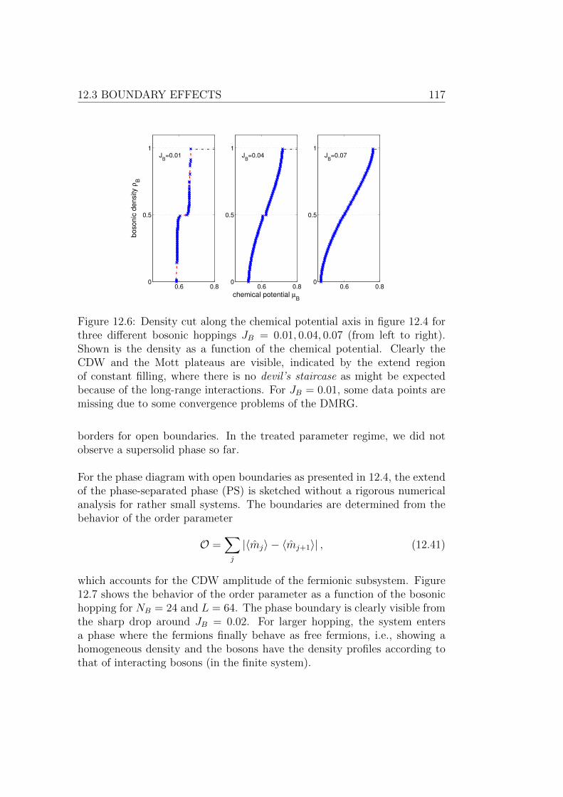
12.3 BOUNDARY EFFECTS 117
0.6 0.80
0.5
1
bosonic
density ρ
B
0.6 0.80
0.5
1
chemical potential µB
0.6 0.80
0.5
1J
B=0.01 J
B=0.04 J
B=0.07
Figure 12.6: Density cut along the chemical potential axis in figure 12.4 forthree different bosonic hoppings JB = 0.01, 0.04, 0.07 (from left to right).Shown is the density as a function of the chemical potential. Clearly theCDW and the Mott plateaus are visible, indicated by the extend regionof constant filling, where there is no devil’s staircase as might be expectedbecause of the long-range interactions. For JB = 0.01, some data points aremissing due to some convergence problems of the DMRG.
borders for open boundaries. In the treated parameter regime, we did notobserve a supersolid phase so far.
For the phase diagram with open boundaries as presented in 12.4, the extendof the phase-separated phase (PS) is sketched without a rigorous numericalanalysis for rather small systems. The boundaries are determined from thebehavior of the order parameter
O =∑j
|〈mj〉 − 〈mj+1〉| , (12.41)
which accounts for the CDW amplitude of the fermionic subsystem. Figure12.7 shows the behavior of the order parameter as a function of the bosonichopping for NB = 24 and L = 64. The phase boundary is clearly visible fromthe sharp drop around JB = 0.02. For larger hopping, the system entersa phase where the fermions finally behave as free fermions, i.e., showing ahomogeneous density and the bosons have the density profiles according tothat of interacting bosons (in the finite system).

118 CHAPTER 12. EFFECTIVE BOSONIC PHASE DIAGRAM
0 0.005 0.01 0.015 0.02 0.025 0.03 0.035 0.04 0.045 0.050
0.5
1
1.5
2
2.5
3
3.5
4
4.5
5
crossover to
free fermions +interacting bosons
phaseseparation
bosonic hopping JB
ord
er
para
mete
r Σ
j |<
mj>
−<
mj+
1>
|
Figure 12.7: Determination of the boundary of the phase separation usingthe order parameter O =
∑j |〈mj〉 − 〈mj+1〉| for open boundary conditions
as function of the bosonic hopping. The transition from the phase separationto the crossover regime is seen by the non-analyticity of the order parameter.Data points are obtained for V = 1.25, JF = 10 and 24 bosons on 64 sitesusing DMRG.
Finally, we mention how the DMRG results in figure 7.3 were obtained. Asdiscussed above, the analytic theory relying on the thermodynamic limitforces the additional (less) particle to be added (removed) close to thecenter. For larger hopping, this state is reproduced by the DMRG, wherethe overall convergence problem of the method due to the highly degeneratesubspace with many close-lying meta-stable states forced us to perform apost-selection of the numerical data. In the figure, only those data pointswhere used, where the numerical results show the additional (less) particleto be situated at the center. This perfectly reproduces the analytic resultsand is well justified. For small hopping, the DMRG data is replaced by datafrom exact diagonalization, since here the boundaries become dominant asdescribed above. All described effects were observed numerically even forrelatively large system sizes L, indicating the trustworthiness of the analyticresults in the thermodynamic limit.
In summary, the derived effective Hamiltonian allows for a full understandingof the physics on the ultrafast-fermion regime.
CHAPTER 13
Conclusion and outlook
The derivation of an effective bosonic Hamiltonian allows for a comprehen-sive understanding of the bosonic phase diagram in the limit of ultrafastfermions. For double half filling, the physics is dominated by inducedlong-range density-density interactions alternating in sign, leading to theemergence of a bosonic charge-density wave phase. Divergences arisingfrom the full decoupling of the fermions are overcome by a renormalizationscheme which includes the back-action of the bosonic CDW on the fermions.Beyond half filling, the induced interactions lead to thermodynamicallyunstable regions in the (µB, JB)-phase diagram, displaying coexistence ofCDW and Mott insulating phases, i.e., a phase separation between CDWand Mott insulator. Numerical results obtained by DMRG for the fullBose-Fermi-Hubbard model are in a reasonable agreement with our analyticpredictions. Application of our effective theory to Bose-Bose of Fermi-Fermimixtures is straightforward.
Mainly focussing on the study of the incompressible and the phase-separatedphases, the nature of the phase transition or crossover for double half fillingremains open. Exponentially decaying first-order correlations even beyondthe numerically detectable extent of the CDW phase indicate further physicalprocesses in this system for larger bosonic hopping. Here bosonization couldgive an understanding of the behavior of the correlation functions as well asthe nature of the phase transition. Furthermore, the question of supersolidityin the effective model is yet unanswered, where the interplay of the inducedpotential and the long-range interactions could lead to new effects. Focussingon low densities %B < 1, the nature of the different phases for larger bosondensities is not studied so far and should give a variety of further phases.
119

Part III
Nonlinear and multi-bandcorrections to the single-bandBose-Fermi-Hubbard model
121


CHAPTER 14
Introduction
Recent experimental results for bosonic atoms in optical lattices [243]revealed that the importance of further contributions in the Hamiltonianbeyond the single-band approximation with nearest-neighbor hopping andlocal two-particle interactions [59]. By means of quantum phase diffusion,the value of the two-body interaction U in the Bose-Hubbard modelwas measured directly. These experiments have also revealed additionalthree- and four-body interaction constants not occurring in the single-bandBose-Hubbard Hamiltonian. Because of the nature of the continuousBose-Hubbard Hamiltonian (1.1), these contributions cannot directly whenintroducing a localized basis. Johnson et al. [244] presented a perturbativeapproach resulting in higher-order interactions. Within this approach, higherBloch bands are incorporated initially1 but eliminated. As a consequence,virtual transitions of the bosons lead to new effective many-body interactions.
For the mixture case, the situation is even more involved. After the firstexperiments on Bose-Fermi mixtures in optical lattices [37, 38] displayinga decrease of the bosonic visibility due to the fermions, the nature of theeffect of the fermions to the bosonic superfluid to Mott-insulator transitionwas discussed controversially. Explanations ranged from localization effectsof bosons induced by fermions [38, Mering2008] to heating because of theadmixture [37, 247]. Numerical results also predicted an opposite behavior,i.e., the enhancement of bosonic visibility because of fermions [88] with amore detailed discussion in [248]. The situation remained unclear until thesystematic study of the dependence of the shift in the bosonic superfluid
1See for instance [245, 246] for discussions of the physics in the higher bands.
123
124 CHAPTER 14. INTRODUCTION
to Mott-insulator transition on the boson-fermion interaction [84] and thesubsequent observation of higher-order interactions measured by means ofquantum phase diffusion in the mixture. This showed, that higher-bandeffects need to be taken into account.
The idea of including further contributions to the Hamiltonian comingfrom higher-band effects can be tackled by two different approaches. Inthe first approach one assumes that the single-particle Wannier functionsare altered due to the fermions and the higher bands [86], which are thencalculated from a self-consistent ansatz. The agreement of these results toexperiments is very reasonable for repulsive boson-fermion interactions (see[84]), but the method suffers from the fact that it can only be applied tothe Mott-insulating state. The second approach, including higher bandsin an elimination scheme leading to an effective single-band Hamiltonian[90, 244, 249] is more promising in this sense, but so far did not resultin reliable predictions due to the usage of the harmonic oscillator ap-proximation. Further methods including higher-band effects are currentlyin development such as a multi-band dynamical mean-field theory [250],slave-boson mean-field theory [251] or Gutzwiller approach [252].
Independently to [90, 244, 249] we here develop an adiabatic eliminationscheme of the higher Bloch bands, resulting in an effective first-band Hamil-tonian. For the renormalized Bose-Hubbard parameters U and JB, extendedby the renormalization due to the fermions, corrections are found in a closedform, including an arbitrary amount of higher bands. All interaction ampli-tudes are calculated from Wannier functions without approximations suchas the harmonic oscillator wavefunctions. Furthermore we found that thereare additional corrections resulting from the interaction term in the originalcontinuous Hamiltonian already within the first band. This allows for a di-rect study of the influence of the interactions on the bosonic superfluid toMott-insulator transition, both in one and three dimensions.

CHAPTER 15
Derivation of the multi-band
Bose-Fermi-Hubbard model
For the derivation of the multi-band Bose-Fermi-Hubbard Hamiltonian wefollow the usual route presented in the introduction in chapter 1. In ourtreatment, the higher bands are incorporated in an adiabatic approximationresulting in a renormalization of the physics in the first band as well as addi-tional nonlinear terms. In this adiabatic elimination, only virtual processesto the empty higher bands are taken into account which corresponds to asecond order perturbation theory in the interband coupling. This secondorder approach is equivalent to the assumption, that higher Bloch bands areuncoupled to each other and it suffices to calculate the effect of an individualband to the renormalization of the first band and finally sum up all higherbands. Thereby, depending on the symmetry, different virtual processes canoccur.
Within this approach, the resulting Hamiltonian for the full multi-band Bose-Fermi-Hubbard model takes the form
H = H1 +∞∑b=2
Hb +∞∑b=2
H1b, (15.1)
where H1 is the Hamiltonian of the first band, Hb the (free) b-th-band Hamil-tonian and H1b couples the first band to the b-th band. For a detailed deriva-tion it is convenient to rewrite the continuous Hamiltonian (1.26) for a mix-
125

126 CHAPTER 15. DERIVATION OF THE MULTI-BAND BFHM
ture of bosons and fermions in the form
H =∑
X∈B,F
∫dzΨ†X(z)
[− ~2
2mX
∆ + V XPot(z)
]ΨX(z)
+gBX
2
∫dzΨ†B(z)Ψ†X(z)ΨX(z)ΨB(z)
.
(15.2)
The notation with X ∈ B,F denoting the species allows for a simplifiedtreatment of the upcoming algebra. The intra- and interspecies interactionconstants are defined as
gBB =4π~2
mB
aBB gBF =4π~2
mR
aBF (15.3)
with mR = mBmF
mB+mFbeing the reduced mass and aBB/BF the intra- and in-
terspecies scattering length, respectively. Whereas in the standard approachthe field operators in (15.2) are expanded in terms of Wannier functions forthe first band only, we here use an expansion to all orders of higher Blochbands:
ΨX(z) =∞∑b=1
∑j
aXb,j wXb (z − ja). (15.4)
For the moment we stick with all bands and make a reduction to a singlehigher band later. a is the lattice spacing of the optical lattice. The operatoraXb,j means the annihilation of a particle (X = B a boson and X = F afermion) in the b-th band on site j and wXb (z − aj) is the correspondingWannier function of the b-th band located at site j.
Using the expansion of the field operator, the full multi-band Bose-Fermi-Hubbard Hamiltonian is given by
H =∑X
∑b1,b2
∑j1,j2
JX;b1,b2j1,j2
(aXb1,j1
)†aXb2,j2 (15.5)
+1
2
∑b1,b2,b3,b4
∑j1,j2,j3,j4
UX;b1b2b3b4j1j2j3j4
(aBb1,j1
)† (aXb2,j2
)†aXb3,j4 a
Bb4,j4
.
The generalized hopping amplitude (still containing local contributions)
JX;j1j2b1b2
=
∫dz wXb1(z − j1a)
[− ~2
2mX
∆ + V XPot(z)
]wXb2(z − j2a), (15.6)
15.1. CONTRIBUTING HOPPING MATRIX ELEMENTS 127
and the generalized interaction amplitudes
UX;j1j2j3j4b1b2b3b4
= gBX
∫dz wBb1(z−j1a)wXb2(z−j2a)wXb3(z−j3a)wBb4(z−j4a) (15.7)
are defined corresponding to the discussion in the introduction in section 1.2.We restrict our model in such a way, that only terms of interest are kept.Furthermore, many of the matrix elements vanish because of the symmetryof the Wannier functions.
15.1 Contributing hopping matrix elements
The generalized hopping amplitude (15.6) incorporates several physical pro-cesses. These are the typical intraband hopping processes (b1 = b2 and|j1 − j2| = 1) and the energy of the particles within a band (b1 = b2 andj1 − j2 = 0). Interband transitions are not present because of the orthogo-nality of the Bloch functions. This gives, as remaining contributions
a) the band energy
∆Xb =
∫dz wXb (z)
[− ~2
2mX
∆ + V XPot(z)
]wXb (z), (15.8)
b) the intraband nearest-neighbor hopping
JXb =
∫dz wXb (z − a)
[− ~2
2mX
∆ + V XPot(z)
]wXb (z). (15.9)
In summary, the part of the multi-band Hamiltonian resulting from the gen-eralized hoppings reads
H =∑X,j,b
JXb
[(aXb,j)†aXb,j+1 +
(aXb,j+1
)†aXb,j
]+ ∆X
b
(aXb,j)†aXb,j, (15.10)
where hopping between sites with |j1 − j2| = 2 is omitted since it is smallcompared to the nearest-neighbor hopping (see figure 1.6). Figure 15.1 showsa graphical representation of the different processes.
15.2 Contributing interaction matrix ele-
ments
a) Discussion of the matrix elements
The discussion for the remaining contributions from the interaction termis more involved. This stems on the one hand side from the large number

128 CHAPTER 15. DERIVATION OF THE MULTI-BAND BFHM
JX
3
JX
1
JX
2
∆X
3
∆2
∆X
1
X
Figure 15.1: Different processes coming from the generalized hopping ampli-tudes depicted for the first three bands. The shaded circles represent eitherbosons or fermions with no difference for the Hamiltonian. ∆X
b is the energyof the b-th band and JXb is the intraband nearest-neighbor hopping in theb-th band.
of possible matrix elements and on the other hand from the simplificationwithin our ansatz. The full calculation of the Hamiltonian without thesesimplifications is of course doable, but due to its complexity the physicalprocesses behind it would become intransparent. To summarize, we calculatethe matrix elements in (15.7) with the following assumption:
All Wannier functions used in (15.7) not coming from the first band,have to come from the same band.
This assumption assures that the irrelevant (in the sense of the adiabaticelimination) contributions are left out. These are for instance, the density-density interaction between higher bands, transitions between the higherbands and transitions from the first to the b1-th band together with atransition from the b2-th to the b3-th band. All these matrix elements donot contribute in the adiabatic elimination in second order. Additionally,
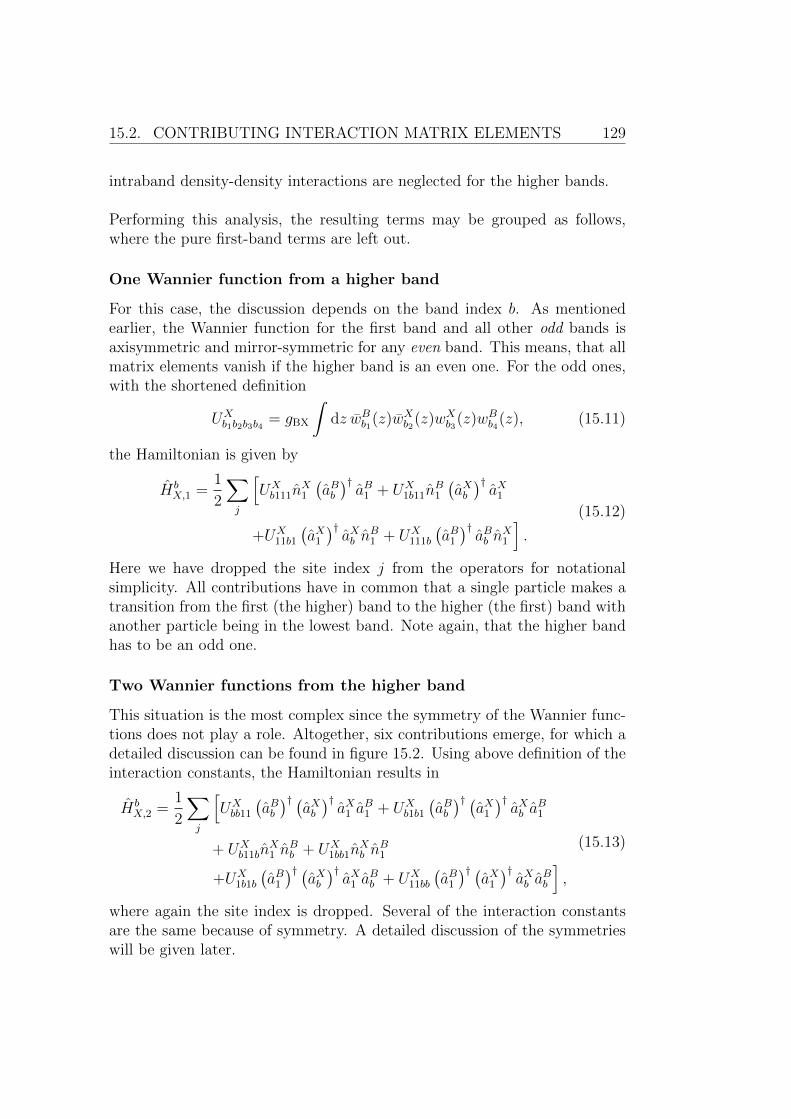
15.2. CONTRIBUTING INTERACTION MATRIX ELEMENTS 129
intraband density-density interactions are neglected for the higher bands.
Performing this analysis, the resulting terms may be grouped as follows,where the pure first-band terms are left out.
One Wannier function from a higher band
For this case, the discussion depends on the band index b. As mentionedearlier, the Wannier function for the first band and all other odd bands isaxisymmetric and mirror-symmetric for any even band. This means, that allmatrix elements vanish if the higher band is an even one. For the odd ones,with the shortened definition
UXb1b2b3b4
= gBX
∫dz wBb1(z)wXb2(z)wXb3(z)wBb4(z), (15.11)
the Hamiltonian is given by
HbX,1 =
1
2
∑j
[UXb111n
X1
(aBb)†aB1 + UX
1b11nB1
(aXb)†aX1
+UX11b1
(aX1)†aXb n
B1 + UX
111b
(aB1)†aBb n
X1
].
(15.12)
Here we have dropped the site index j from the operators for notationalsimplicity. All contributions have in common that a single particle makes atransition from the first (the higher) band to the higher (the first) band withanother particle being in the lowest band. Note again, that the higher bandhas to be an odd one.
Two Wannier functions from the higher band
This situation is the most complex since the symmetry of the Wannier func-tions does not play a role. Altogether, six contributions emerge, for which adetailed discussion can be found in figure 15.2. Using above definition of theinteraction constants, the Hamiltonian results in
HbX,2 =
1
2
∑j
[UXbb11
(aBb)† (
aXb)†aX1 a
B1 + UX
b1b1
(aBb)† (
aX1)†aXb a
B1
+ UXb11bn
X1 n
Bb + UX
1bb1nXb n
B1
+UX1b1b
(aB1)† (
aXb)†aX1 a
Bb + UX
11bb
(aB1)† (
aX1)†aXb a
Bb
],
(15.13)
where again the site index is dropped. Several of the interaction constantsare the same because of symmetry. A detailed discussion of the symmetrieswill be given later.
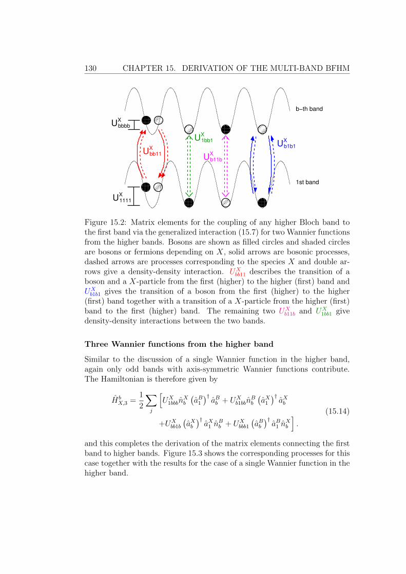
130 CHAPTER 15. DERIVATION OF THE MULTI-BAND BFHM
X
bb11U X
b11bU
X
1bb1U
1111
XU
X
b1b1U
bbbb
XU
1st band
b−th band
Figure 15.2: Matrix elements for the coupling of any higher Bloch band tothe first band via the generalized interaction (15.7) for two Wannier functionsfrom the higher bands. Bosons are shown as filled circles and shaded circlesare bosons or fermions depending on X, solid arrows are bosonic processes,dashed arrows are processes corresponding to the species X and double ar-rows give a density-density interaction. UX
bb11 describes the transition of aboson and a X-particle from the first (higher) to the higher (first) band andUXb1b1 gives the transition of a boson from the first (higher) to the higher
(first) band together with a transition of a X-particle from the higher (first)band to the first (higher) band. The remaining two UX
b11b and UX1bb1 give
density-density interactions between the two bands.
Three Wannier functions from the higher band
Similar to the discussion of a single Wannier function in the higher band,again only odd bands with axis-symmetric Wannier functions contribute.The Hamiltonian is therefore given by
HbX,3 =
1
2
∑j
[UX
1bbbnXb
(aB1)†aBb + UX
b1bbnBb
(aX1)†aXb
+UXbb1b
(aXb)†aX1 n
Bb + UX
bbb1
(aBb)†aB1 n
Xb
].
(15.14)
and this completes the derivation of the matrix elements connecting the firstband to higher bands. Figure 15.3 shows the corresponding processes for thiscase together with the results for the case of a single Wannier function in thehigher band.
15.2. CONTRIBUTING INTERACTION MATRIX ELEMENTS 131
X
b111UX
b1bbUX
1bbbU1b11
XU
1st band
b−th band
odd
even band
Figure 15.3: Matrix elements for the coupling of the odd higher bands tothe first band for one or three Wannier functions from the higher bands viathe generalized interaction (15.7). The notation is the same as in figure15.2. Additionally, the bidirectional arrows are local density contributionsas stated in the main text. All processes feature the interband transition ofa single particle together with a density interaction, either from the higheror the first band.

132 CHAPTER 15. DERIVATION OF THE MULTI-BAND BFHM
b) Complete Hamiltonian for the b-th band from theinteraction
Combining all results for the different cases and exploiting the symmetriesof the generalized coupling constants, the full Hamiltonian for the couplingof the first to the b-th band is given by
HbX = Hb
X,1 + HbX,2 + Hb
X,3 + HbX,4
=∑j
[UXb11b
2nX1,jn
Bb,j +
UX1bb1
2nXb,jn
B1,j
+UXbb11
2
((aBb,j)† (
aXb,j)†aX1,j a
B1,j +
(aBb,j)† (
aX1,j)†aXb,j a
B1,j
+(aB1,j)† (
aXb,j)†aX1,j a
Bb,j +
(aB1,j)† (
aX1,j)†aXb,j a
Bb,j
)]∣∣∣∣∣all bands
+∑j
[UXb111
2
(nX1,j
(aBb,j)†aB1,j +
(aB1,j)†aBb,jn
X1,j
)+UX
1b11
2
(nB1,j
(aXb,j)†aX1,j
+(aX1,j)†aXb,jn
B1,j
)+UX
1bbb
2
(nXb,j
(aB1,j)†aBb,j +
(aBb,j)†aB1,jn
Xb,j
)
+UXb1bb
2
(nBb,j
(aX1,j)†aXb,j +
(aXb,j)†aX1,jn
Bb,j
)]∣∣∣∣∣odd bands
.
(15.15)
For the interaction amplitudes, the following symmetry relations hold andhave been used:
UXabcd = UX
dbca = UXacbd. (15.16)
This results from the structure of the Wannier functions which are real val-ued.
15.3 Full (relevant) multi-band Bose-Fermi-
Hubbard Hamiltonian
With the above results, we are able to pin down the full multi-band Bose-Fermi-Hubbard model. Using Uabcd := UB
abcd for the boson-boson interactionand Vabcd = UF
abcd for the boson-fermion interaction, the Hamiltonian includ-ing the first band as well as all relevant couplings to an arbitrary higher band
15.3. FULL (RELEVANT) MULTI-BAND BFHM 133
is given by
Hb = H free1st + H free
bth + H int, anybth + H int, odd
bth (15.17)
with the Hamiltonian of the 1st
H free1st = JB1
∑j
(a†1,j a1,j+1 + a†1,j+1a1,j
)+U1111
2
∑j
n1,j(n1,j − 1)
+ JF1∑j
(c†1,j c1,j+1 + c†1,j+1c1,j
)+V1111
2
∑j
n1,jm1,j
+ ∆B1
∑j
n1,j + ∆F1
∑j
m1,j
(15.18)
and the free Hamiltonian of the b-th band
H freebth = JBb
∑j
(a†b,j ab,j+1 + a†b,j+1ab,j
)+ ∆B
b
∑j
nb,j
+ JFb∑j
(c†b,j cb,j+1 + c†b,j+1cb,j
)+ ∆F
b
∑j
mb,j
(15.19)
whith b ∈ 2 . . .∞, the interaction Hamiltonian
H int, anybth =
∑j
Ubb11
2
[(a†b,j
)2
a21,j + 4nb,jn1,j +
(a†1,j
)2
a2b,j
]
+∑j
[Vb11b
2m1,jnb,j +
V1bb1
2mb,jn1,j
+Vbb11
2
(a†b,j c
†b,j c1,j a1,j + a†b,j c
†1,j cb,j a1,j
+ a†1,j c†b,j c1,j ab,j + a†1,j c
†1,j cb,j ab,j
)](15.20)
coupling any band and
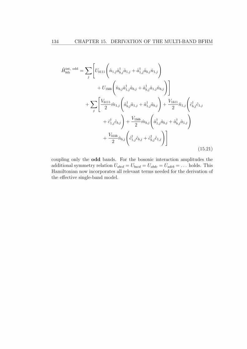
134 CHAPTER 15. DERIVATION OF THE MULTI-BAND BFHM
H int, oddbth =
∑j
[Ub111
(n1,j a
†b,j a1,j + a†1,j ab,jn1,j
)
+ U1bbb
(nb,j a
†1,j ab,j + a†b,j a1,jnb,j
)]
+∑j
[Vb111
2m1,j
(a†b,j a1,j + a†1,j ab,j
)+V1b11
2n1,j
(c†b,j c1,j
+ c†1,j cb,j
)+V1bbb
2mb,j
(a†1,j ab,j + a†b,j a1,j
)
+Vb1bb
2nb,j
(c†1,j cb,j + c†b,j c1,j
)](15.21)
coupling only the odd bands. For the bosonic interaction amplitudes theadditional symmetry relation Uabcd = Ubacd = Uabdc = Uadcb = . . . holds. ThisHamiltonian now incorporates all relevant terms needed for the derivation ofthe effective single-band model.

CHAPTER 16
Adiabatic elimination of higher bands and
nonlinear corrections
16.1 Adiabatic elimination and effective
single-band Hamiltonian
With the full Hamiltonian (15.17), the adiabatic elimination follows the sameroute as performed in chapter 8 for the case of fast fermions, but, instead oftracing out the fermions, the trace is performed over the higher bands. TheHamiltonian is split up into a free and an interaction part, defined as
Hb = Hfree + HI (16.1)
with
Hfree = H free1st + H free
bth (16.2)
HI = H int, anybth + H int, odd
bth . (16.3)
In the interaction picture, the dynamics of the free part is incorporated bythe time dependent interaction Hamiltonian HI(τ) = e−
i~ Hfreeτ HI e
i~ Hfreeτ
and the scattering matrix of the full system is given by
S = T exp
− i~∞∫
−∞
dτHI(τ)
. (16.4)
Tracing over the higher-band degrees of freedom assuming vacuum in thatband and using the cumulant expansion (8.7) up to second order as described
135

136 CHAPTER 16. ADIABATIC ELIMINATION OF HIGHER BANDS
in chapter 8, the effective scattering matrix for the lowest band reads
S1steff = T exp
− i~∞∫
−∞
dτ
(− i
2~
) ∞∫−∞
dT 〈〈T HI(τ + T )HI(τ)〉〉bth
.
(16.5)From the first order in the cumulant expansion no contributions occur sinceeither the number of creation and annihilation operators in the higher bandapplied on the vacuum state is unequal or the higher band operators arenormal ordered.
The calculation of the second order cumulant is rather lengthy and can befound in appendix B.1. Together with a subsequent Markov approximationalready used in chapter 81, the effective Hamiltonian for the first-band Bose-Fermi-Hubbard model is given by
Heff1st = H free
1st +∑jd
U2bb11IdBB,b
2
(a†j+d
)2
a2j +
V 2bb11IdBF,b
4a†j+dc
†j+dcj aj
+ U2b111IdB,b a
†j+dnj+dnj aj +
Ub111Vb111IdB,b2
mj+da†j+dnj aj
+Vb111Ub111IdB,b
2a†j+dnj+dmj aj +
V 2b111IdB,b
4mj+da
†j+dmj aj
+V 2
1b11IdF,b4
nj+dc†j+dnj cj
.
(16.6)
Here, explicit distinction between even and odd bands is omitted for nota-tional simplicity. The first two terms account for any band whereas all otherterms come into play only for odd bands2. In the Hamiltonian, the timeintegrals over the bosonic and fermionic correlators are defined as
IdB,b = − i~
∞∫0
dT CTB,b(d), IdBB,b = − i~
∞∫0
dT(CTB,b(d)
)2, (16.7)
IdF,b = − i~
∞∫0
dT CTF,b(d), IdBF,b = − i~
∞∫0
dT CTF,b(d)CTB,b(d), (16.8)
1The Markov approximation here is justified because the absolute value of the hoppingamplitudes in the higher bands are larger than in the first band. See [110, 253] and section1.2 for details.
2As a rule of thumb, terms with an odd number of “b”’s in the interaction amplitudesU and V only stem from odd bands.

16.2. NONLINEAR CORRECTIONS FOR THE FIRST BAND 137
with
CTB,b(d) = 〈ab,j+d(τ + T )a†b,j(τ)〉bth, CTF,b(d) = 〈cb,j+d(τ + T )c†b,j(τ)〉bth.(16.9)
As shown in B.2, these evaluate to
〈ab,j+d(τ + T )a†b,j(τ)〉bth =1
L
∑k
e−2πid kL e
i~Tε
B,bk (16.10)
〈cb,j+d(τ + T )c†b,j(τ)〉bth =1
L
∑k
e−2πid kL e
i~Tε
F,bk (16.11)
which, together with the time integration, give
IdX,b =1
π
π∫0
dξcos(dξ)
εX,b(ξ)(16.12)
IdBX,b =1
π2
π∫0
dξ
π∫0
dξ′cos(dξ) cos(dξ′)
εB,b(ξ) + εX,b(ξ)(16.13)
in the thermodynamic limit3. εX,b(ξ) = 2JXb cos(ξ) + ∆Xb is the energy of a
free particle (either bosonic or fermionic) in the higher band and the furtherdetails can be found in appendix B.3.
16.2 Nonlinear corrections for the first band
From equation (16.6), the structure of the effective first-band Hamiltoniancan be seen. As one can see, for a proper derivation of the effective first-bandHamiltonian, the approximations commonly used for the first-band interac-tion amplitudes are too stringent and need to be expanded. Since nonlocaldensity-density interactions and density-mediated hopping processes are adirect consequence of the couplings to higher bands, these should also beincluded in the pure first-band treatment. Doing so, the generalized inter-action (15.7) needs to be extended by terms featuring either a two-particle(equal distance) hopping
U2d1111
(a†j+d
)2
a2j , (16.14)
V 2d1111 a
†j+dc
†j+dcj aj, (16.15)
3As in part II, the thermodynamic limit is reached for L → ∞ by setting ξ = kL and
changing 1L
∑k to
∫dξ.
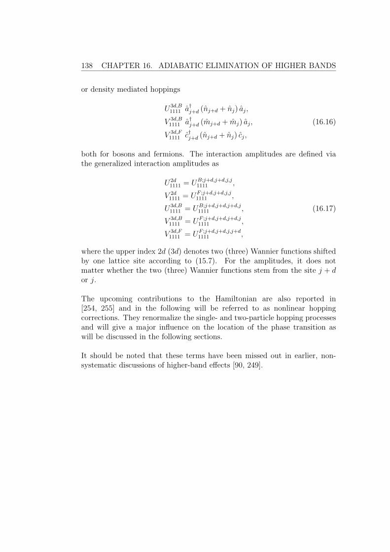
138 CHAPTER 16. ADIABATIC ELIMINATION OF HIGHER BANDS
or density mediated hoppings
U3d,B1111 a†j+d (nj+d + nj) aj,
V 3d,B1111 a†j+d (mj+d + mj) aj, (16.16)
V 3d,F1111 c†j+d (nj+d + nj) cj,
both for bosons and fermions. The interaction amplitudes are defined viathe generalized interaction amplitudes as
U2d1111 = UB;j+d,j+d,j,j
1111 ,
V 2d1111 = UF ;j+d,j+d,j,j
1111 ,
U3d,B1111 = UB;j+d,j+d,j+d,j
1111 , (16.17)
V 3d,B1111 = UF ;j+d,j+d,j+d,j
1111 ,
V 3d,F1111 = UF ;j+d,j+d,j,j+d
1111 ,
where the upper index 2d (3d) denotes two (three) Wannier functions shiftedby one lattice site according to (15.7). For the amplitudes, it does notmatter whether the two (three) Wannier functions stem from the site j + dor j.
The upcoming contributions to the Hamiltonian are also reported in[254, 255] and in the following will be referred to as nonlinear hoppingcorrections. They renormalize the single- and two-particle hopping processesand will give a major influence on the location of the phase transition aswill be discussed in the following sections.
It should be noted that these terms have been missed out in earlier, non-systematic discussions of higher-band effects [90, 249].

16.3. FULL (EFFECTIVE) SINGLE-BAND BFHM 139
16.3 Full effective single-band Bose-Fermi-
Hubbard Hamiltonian
In summary, the full effective Hamiltonian for the first band reduced tohopping contributions and local interactions is given by
Heff =∑j
[U3
6nj (nj − 1) (nj − 2) +
V3
2mjnj (nj − 1)
+U2
2nj (nj − 1) + V njmj
]+∑j
∆B1 nj +
∑j
∞∑d=−∞d6=0
a†j+d JB[d; nj, nj+d, mj, mj+d] aj
+∑j
∆F1 mj +
∑j
∞∑d=−∞d6=0
c†j+d JF [d; nj, nj+d] cj
+∑j
∞∑d=−∞d6=0
[J
(2)B (d)
(a†j+d
)2
a2j + J
(2)F (d) a†j+dc
†j+dcj aj
].
(16.18)
For a definition of the constants refer to appendix B.4. In comparisonto the usual single-band picture, the emergence of some new terms canbe seen. The inclusion of the higher bands leads on the one hand to arenormalization of the local interaction amplitudes and on the other handto (long-range), density mediated hopping processes as well as correlatedtwo-particle tunneling. Most prominent is the appearance of the three-bodyinteraction U3 which has been measured experimentally recently by meansof quantum phase diffusion [243]. Using the method for the calculation ofthe Wannier functions presented in the next chapter, the value of U3 turnsout to be of the same sign as seen in the experiments (and analytic theory in[244] using the harmonic oscillator approximation), whereas the ratio U3/U2
is only correct up to an order of magnitude. This is not surprising, sincethere are further contributions of higher order in the interband couplingnot included in our second-order approach. Nevertheless, the accordance ofthis simple quantity already shows that our used method allow for a properdescription of the influence of the higher bands.
In order to discuss the phase transition of the bosonic subsystem, wefurthermore reduce the Hamiltonian to the relevant parts. These are,compared to the pure single-band nonlinear Bose-Hubbard model the on-site

140 CHAPTER 16. ADIABATIC ELIMINATION OF HIGHER BANDS
interaction as well as the nearest-neighbor hopping. We start our discussioncoming from the Mott insulator, thus the local number of particles isapproximately given by the integer filling of the system, i.e., 〈nj〉 ≈ n. Thisis used to replace the number operators in the hopping terms by the fillingn, giving a reasonable approximation for the calculation of the renormalizedhoppings. For the fermionic species, we also replace the number operatorby the fermionic filling mj → m = 1, assuming a homogeneous filling ofthe fermions in the lattice. Having an experimental realization with coldatoms in mind, this specific case is a valid assumption in the center of theharmonic trap at least for attractive inter-species interactions. It shouldbe valid however also for sufficiently small inter-species repulsion. Thisassumption is also supported by the results from [84], where the fermionicdensity did not influence the transition from a Mott-insulator to a superfluid(for medium and large filling). It also agrees with the result in [86] which isbased on this assumption, showing a good agreement to the experimentalresults. All further contributions in the Hamiltonian as the three-particleinteraction and two-particle hoppings are neglected in the following.
With these approximations, the renormalized Bose-Hubbard Hamiltonian isgiven by
Heff = −J [n,m]∑j
(a†j aj+1 + a†j+1aj
)+U [n,m]
2
∑j
nj (nj − 1) (16.19)
with
J [n,m] = JB1 + 2nU3d,B
1111
2+ 2m
V 3d,B1111
2(16.20)
+∑b>1b odd
I1B,b
[U2b111 n
2 + 2Ub111Vb111
2nm+
V 2b111
4m2]
U [n,m] = U1111 +∑b>1
U2bb11I0
BB,b +∑b>1b odd
2 U2b111I0
B,b (16.21)
+m∑b>1b odd
[2 Ub111Vb111I0
B,b +V 2
1b11I0F,b
2
]
For the correlator integrals I0X,b and I1
X,b, equation (16.12), simple expressions

16.3. FULL (EFFECTIVE) SINGLE-BAND BFHM 141
can be found:
I0X,b =
1√(∆X
b )2 − (2JXb )2
I1X,b =
1
2JXb(1−∆X
b I0X,b
) . (16.22)
This Hamiltonian serves as the starting point for the discussion of the in-fluence of the boson-fermion interaction on the Mott-insulator to superfluidtransition as studied in the experiments in [37, 38, 84]. This will be doneafter a short summary of the relevant experimental parameters and theirimplications on the discussions so far.

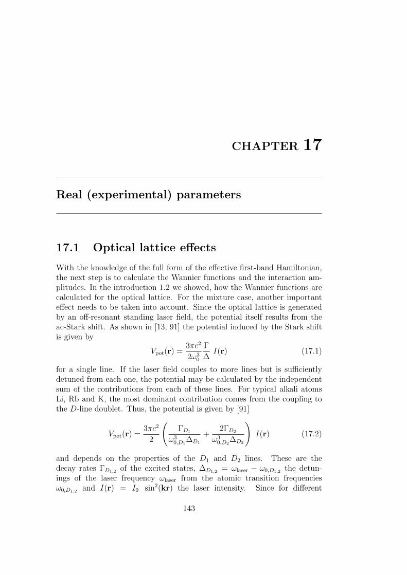
CHAPTER 17
Real (experimental) parameters
17.1 Optical lattice effects
With the knowledge of the full form of the effective first-band Hamiltonian,the next step is to calculate the Wannier functions and the interaction am-plitudes. In the introduction 1.2 we showed, how the Wannier functions arecalculated for the optical lattice. For the mixture case, another importanteffect needs to be taken into account. Since the optical lattice is generatedby an off-resonant standing laser field, the potential itself results from theac-Stark shift. As shown in [13, 91] the potential induced by the Stark shiftis given by
Vpot(r) =3πc2
2ω30
Γ
∆I(r) (17.1)
for a single line. If the laser field couples to more lines but is sufficientlydetuned from each one, the potential may be calculated by the independentsum of the contributions from each of these lines. For typical alkali atomsLi, Rb and K, the most dominant contribution comes from the coupling tothe D-line doublet. Thus, the potential is given by [91]
Vpot(r) =3πc2
2
(ΓD1
ω30,D1
∆D1
+2ΓD2
ω30,D2
∆D2
)I(r) (17.2)
and depends on the properties of the D1 and D2 lines. These are thedecay rates ΓD1,2 of the excited states, ∆D1,2 = ωlaser − ω0,D1,2 the detun-ings of the laser frequency ωlaser from the atomic transition frequenciesω0,D1,2 and I(r) = I0 sin2(kr) the laser intensity. Since for different
143

144 CHAPTER 17. REAL (EXPERIMENTAL) PARAMETERS
atomic species (in general even for different isotopes but here the effect ismarginal), the atomic transition frequencies differ, i.e., all species in theoptical setup experience different amplitudes of the optical lattices1. Thisinfluences the Wannier functions which we take into account in the following.
Conveniently, all energies in the system are normalized to the so-called recoilenergy, which is defined as the change in kinetic energy of an atom upon ab-sorption of a photon from the optical lattice laser. In our case, we normalizeto the recoil energy of the bosonic species, given by
EBrec =
~2k2
2mB
, (17.3)
with the wavenumber k of the optical lattice. It is useful to rewrite theoptical lattice potential for the fermionic atoms with respect to the bosonicoptical lattice. Following the notation in [110], the optical lattice potentialfor the second (fermionic) species is written in the form
V Fpot(r) = ηF sin2(kr) (17.4)
where ηF = 3πc2
2
(ΓFD1
(ωF0,D1
)3∆F
D1
+2ΓF
D2
(ωF0,D2
)3∆F
D2
)I0. The definition of the am-
plitude ηF allows for an easy connection of the fermionic potential to thebosonic one as
ηF =
ΓFD1
(ωF0,D1
)3∆F
D1
+2ΓF
D2
(ωF0,D2
)3∆F
D2
ΓBD1
(ωB0,D1
)3∆B
D1
+2ΓB
D2
(ωB0,D2
)3∆B
D2
ηB = f ηB. (17.5)
The prefactor f connects the bosonic and fermionic potential depth. For thecalculation of the prefactor, the values for the different atomic species canbe found for typical isotopes in [256, 257, 258] or at the NIST2 homepage[259].
For the calculation of the Wannier functions for the fermions using theSchrodinger equation[
− ~2
2mF
∆ + ηF sin2(kr)
]Φ(r) = E Φ(r), (17.6)
1If the one species is red, the other species blue detuned, the two species do not justexperience different amplitudes but also different positions of the minima of the potential.
2National Institute of Standards and Technology

17.1. OPTICAL LATTICE EFFECTS 145
the normalization to the bosonic recoil energy leads to additional fac-tors which originate from the mass difference. This gives the fermionicSchrodinger equation[
− ~2
2mB
∆ +mF
mB
f ηB sin2(kr)
]Φ(r) =
mF
mB
E Φ(r). (17.7)
Note, that the depth of the optical lattice potential for the fermions is alteredby a prefactor mF
mBf compared to the bosonic one and the energy of the
fermionic system is altered by mF
mB. This factor in the energy demands a
careful treatment of the intraband hopping JFb and the band energy ∆Fb . For
a fixed amplitude η of an optical lattice (in units of the recoil energy3), theyare given by the Fourier transform of the energy dispersion respectively themean value as shown in section 1.2. This gives
Jb =1
2
1∫−1
dp Eb(p) e−iπp ∆b =
1
2
1∫−1
dp Eb(p), (17.8)
where Eb(p) is the dispersion of the b-th band. For the calculation of theenergy dispersion, the free Hamiltonian (17.6) was normalized to the recoilenergy, giving, for the fermionic species, the hopping and the band energywith respect to the fermionic recoil energy. In bosonic units, the factor
EFrec
EBrec
=mB
mF
(17.9)
needs to be included, giving the dependence of the hopping and the bandenergy as a function of ηB (by using the prefactor f mF
mB) in units of the
bosonic recoil energy.
At this point, we specify the experimental system. In the following, weanalyze the experiment reported in [84] and use the parameters given there.The experiment treats the visibility of the bosonic cloud in the optical latticeas a function of the boson-fermion scattering length aBF tuned by a Feshbachresonance [13, 260, 261]. A mixture of bosonic 87Rb and fermionic 40K iscooled and put into an optical lattice with λL = 755 nm. For Rubidium[258] and Potassium [259, 262], the transition wavelengths and decay rates
3Here we discuss the general case and therefore remove any index B or F .
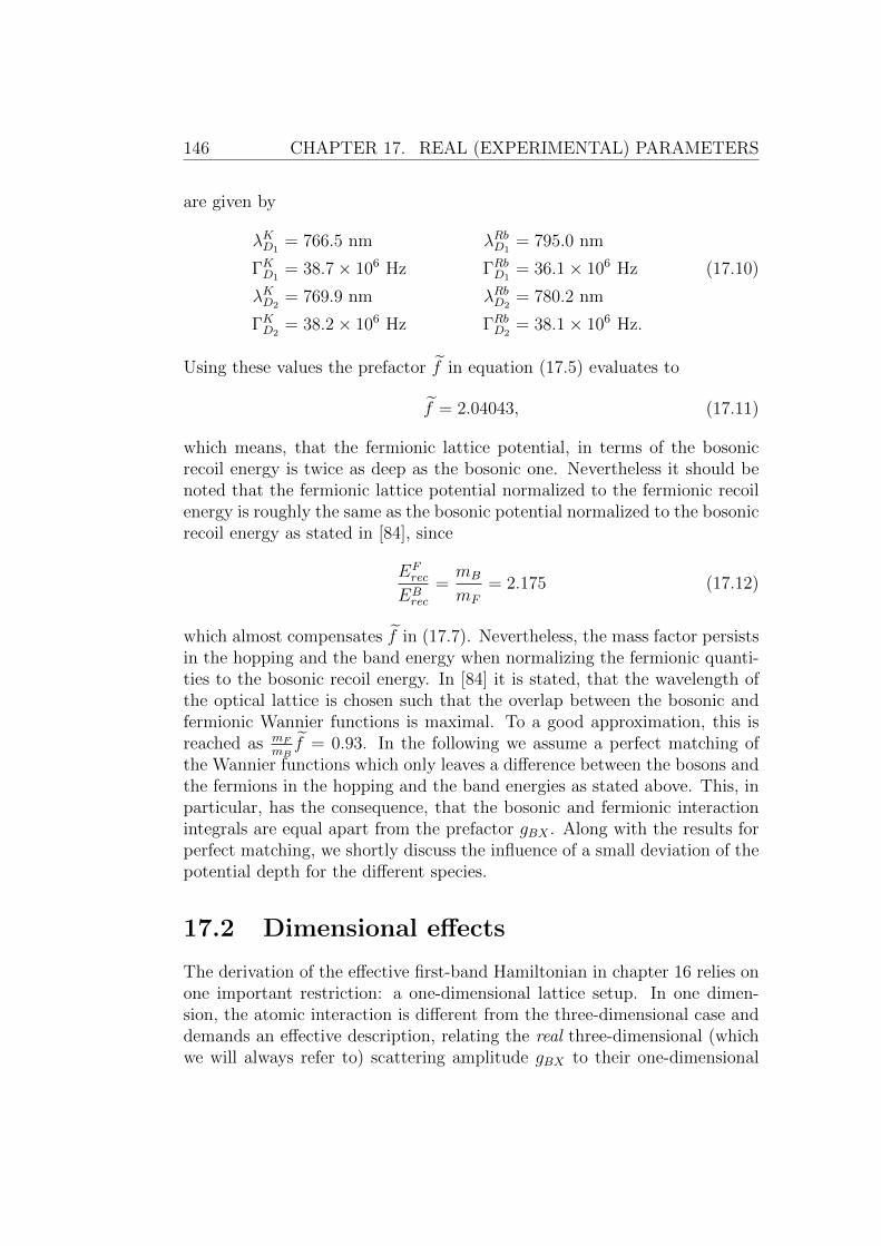
146 CHAPTER 17. REAL (EXPERIMENTAL) PARAMETERS
are given by
λKD1= 766.5 nm λRbD1
= 795.0 nm
ΓKD1= 38.7× 10⁶ Hz ΓRbD1
= 36.1× 10⁶ Hz (17.10)
λKD2= 769.9 nm λRbD2
= 780.2 nm
ΓKD2= 38.2× 10⁶ Hz ΓRbD2
= 38.1× 10⁶ Hz.
Using these values the prefactor f in equation (17.5) evaluates to
f = 2.04043, (17.11)
which means, that the fermionic lattice potential, in terms of the bosonicrecoil energy is twice as deep as the bosonic one. Nevertheless it should benoted that the fermionic lattice potential normalized to the fermionic recoilenergy is roughly the same as the bosonic potential normalized to the bosonicrecoil energy as stated in [84], since
EFrec
EBrec
=mB
mF
= 2.175 (17.12)
which almost compensates f in (17.7). Nevertheless, the mass factor persistsin the hopping and the band energy when normalizing the fermionic quanti-ties to the bosonic recoil energy. In [84] it is stated, that the wavelength ofthe optical lattice is chosen such that the overlap between the bosonic andfermionic Wannier functions is maximal. To a good approximation, this isreached as mF
mBf = 0.93. In the following we assume a perfect matching of
the Wannier functions which only leaves a difference between the bosons andthe fermions in the hopping and the band energies as stated above. This, inparticular, has the consequence, that the bosonic and fermionic interactionintegrals are equal apart from the prefactor gBX . Along with the results forperfect matching, we shortly discuss the influence of a small deviation of thepotential depth for the different species.
17.2 Dimensional effects
The derivation of the effective first-band Hamiltonian in chapter 16 relies onone important restriction: a one-dimensional lattice setup. In one dimen-sion, the atomic interaction is different from the three-dimensional case anddemands an effective description, relating the real three-dimensional (whichwe will always refer to) scattering amplitude gBX to their one-dimensional

17.2. DIMENSIONAL EFFECTS 147
counterpart. Under the assumption of a three-dimensional gas in a strongcigar-shaped trap, Olshanii derived the effective one-dimensional scatteringamplitude [263] for a point like interaction between two atoms. With astrong confinement of the atomic cloud in the transversal direction givenby ω⊥ ω‖, the effective one-dimensional scattering amplitude g1D for atwo-particle interaction4 results in
g1D =g3D
πl2⊥
1
1 + ζ(12) a3D
l⊥
. (17.13)
g3D = 2π~2mR
a3D is the scattering amplitude, mR is the reduced mass of thescattering partners, a3D is the scattering length for the treated scatteringprocess in three dimensions and ζ(x) is the Riemann-Zeta function. Becauseof the strong harmonic confinement in the transversal direction, the value
of the oscillator length l⊥ =√
~µω⊥
is of major importance. The transversal
trap frequency is typically in the range of some kHz [63, 264, 265] dependingon the actual realization of the trap. In the following we use the value ofω⊥ ≈ 80kHz given in [264].
For the calculation of the one-dimensional scattering amplitude, the lastmissing ingredient is the three-dimensional scattering length. For the Rb-Rbinteraction, the experimental (background) scattering length is measured tobe a87Rb = aBB = 108 a0, with the Bohr radius a0 = 0.053nm [266]. Theboson-fermion scattering length aBF from now on serves as a free, tunableparameter, used to study the influence of the fermions to the bosonicsuperfluid to Mott-insulator transition. The background value and referencepoint for the mixture of 87Rb and 40K is aBF = −205 a0, i.e., is attractive[37, 38].
In the derivation of the effective one-dimensional scattering amplitude g1D itis assumed, that the two particles which scatter experience the same transver-sal confinement. For a homonuclear scattering process, this is true. For theheterogeneous scattering between bosons and fermions, this does not neces-sarily hold. But usually, the cigar-shaped optical potential is created by astrong far off-resonant dipole trap. The large detuning to both, bosons andfermions then leads roughly to the same transversal confinement for bothspecies. This is seen in our situation by comparing the intensities of theoptical dipole trap, calculated using equation (17.5) for a typical laser setup
with λdipole = 1030 nm. The prefactor f ≈ 0.9 turns out to be close to
4Here we omit the index X since the discussion does not depend on it.

148 CHAPTER 17. REAL (EXPERIMENTAL) PARAMETERS
n = 1 n = 2 n = 3 n = 4
1D 4.65 7.86 11.04 14.23
3D 29.34 49.83 70.11 90.32
Table 17.1: Critical ratio U/J in the Bose-Hubbard model for the Mott-insulator to superfluid transition in one and three dimensions. 1D: resultsfrom strong-coupling theory [97]. 3D: For the first lobe, the exact quantummonte-carlo result from [267] is used. For the higher lobes, analytic fieldtheory results from [173] are used. For details see the main text.
unity and therefore, both species are attributed to the same dipole trappinggeometry and the assumptions in the derivation of the scattering strengthare valid even in the mixture case.
17.3 Bose-Hubbard phase transition
Before we discus the net effect of the fermions, the higher bands andnonlinear hopping corrections on the phase diagram of the Bose-Hubbardmodel, we shortly summarize the results for the Mott-insulator to superfluidtransition in the pure bosonic system. This serves as an example whichshows how to calculate the transition point of the phase transition and givesthe starting point for the analysis of the shift of the transition as a functionof the boson-fermion scattering length aBF .
The key feature for the determination of the Mott-insulator to superfluidtransition is the ratio of interaction to kinetic energy, U/J . Several analytic[14, 97, 170, 173, 181, 240] and numerical [183, 211, 267] results for thistransition exist, with slight deviations coming from the different methodsbut all are in good agreement with each other. For the experiments, thetransition is found by calculating the interaction amplitude U and thehopping amplitude J as a function of the optical lattice depth η and seekfor the value of η, at which the ratio U/J equals the analytic or numericresults for the transition point for a fixed filling n. Here we make use of thestrong-coupling results from [97] in one dimension as well as a combination

17.3. BOSE-HUBBARD PHASE TRANSITION 149
8 9 10 11.76 13.61 14.88 15.86 17 1810
20
30
40
50
60
708090
100
potential depth η [Erec
]
U/J
B
n=4
n=3
n=2
n=1
Figure 17.1: Ratio U/J as a function of the optical lattice depth for a three-dimensional setup. The critical point, where the Mott-insulator to superfluidtransition occurs is found at the place, where U/J reaches the critical valuedetermined by numerical or analytic methods. Also shown are the transitionpoints for the first four Mott lobes.
of the analytic results from [173] and the numerical ones from [267] inthree dimension. Table 17.1 shows a list of the transition points in oneand three dimensions. For three dimensions, the critical ratio for n = 1lobe is taken from the high precision quantum monte-carlo result in [267].The other lobes are calculated with the analytic result in [173], where theoverestimation from the approximative field theory of about 3% for thefirst lobe is also substracted from the analytic results for the higher lobes.These values are in good agreement with the numerical results from [170]and are preferable to be used because they are given in a closed analytic form.
Figure 17.1 shows how the transition point is determined as a function of thelattice depth η as described in [15]. Plotting the ratio U/J as a function ofη, the crossing point of this ratio with the calculated transition points fromtable 17.1 gives the position of the Mott-insulator to superfluid transition forthe different Mott lobes. For the pure Bose-Hubbard model plotted in figure17.1, this prediction is in reasonable agreement with the experimental resultof ηcrit ≈ 12.5 Erec [15]. Using this method, the influence of the differentcorrections to the pure Bose-Hubbard model is studied in the next chapter.

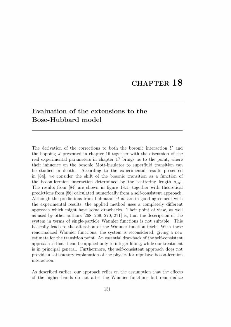
CHAPTER 18
Evaluation of the extensions to the
Bose-Hubbard model
The derivation of the corrections to both the bosonic interaction U andthe hopping J presented in chapter 16 together with the discussion of thereal experimental parameters in chapter 17 brings us to the point, wheretheir influence on the bosonic Mott-insulator to superfluid transition canbe studied in depth. According to the experimental results presentedin [84], we consider the shift of the bosonic transition as a function ofthe boson-fermion interaction determined by the scattering length aBF .The results from [84] are shown in figure 18.1, together with theoreticalpredictions from [86] calculated numerically from a self-consistent approach.Although the predictions from Luhmann et al. are in good agreement withthe experimental results, the applied method uses a completely differentapproach which might have some drawbacks. Their point of view, as wellas used by other authors [268, 269, 270, 271] is, that the description of thesystem in terms of single-particle Wannier functions is not suitable. Thisbasically leads to the alteration of the Wannier function itself. With theserenormalized Wannier functions, the system is reconsidered, giving a newestimate for the transition point. An essential drawback of the self-consistentapproach is that it can be applied only to integer filling, while our treatmentis in principal general. Furthermore, the self-consistent approach does notprovide a satisfactory explanation of the physics for repulsive boson-fermioninteraction.
As described earlier, our approach relies on the assumption that the effectsof the higher bands do not alter the Wannier functions but renormalize
151

152 18. EVALUATION OF THE EXTENDED BHM
Figure 18.1: Experimental results for the shift of the bosonic Mott-insulatorto superfluid transition taken from [84]. Data points (blue and yellow) arefrom the same experiment with different fermion numbers, the lines are var-ious theoretical predictions. For details see [84] and [86].
the parameters in the Hamiltonian itself and provide new nonlinear terms.This approach is similar to the one chosen in Ref. [90, 244, 249]. Themain difference between our approach and the mentioned works is, that allthree rely on the harmonic oscillator assumption. Furthermore, they restrictthemselves to a rather small number of higher bands. Though these assump-tions easily allow to apply the higher-band corrections to dimensions largerthan one, they are inaccurate when comparing to the experimental resultsas the correct form of the Wannier functions is important as demonstratedin this chapter. For instance, the ground state of a harmonic oscillator isa strictly positive function, while the Wannier function in the lowest bandhas small negative parts with a sizeable effect on overlap integrals involvingWannier functions of different sites. Finally, nonlinear hopping correctionshave been neglected in [90, 244, 249] which play an important role however.
After these initial comments, we first discuss our results for one dimensionand afterward give some preliminary results for three dimensions.

18.1. ONE-DIMENSIONAL LATTICE 153
18.1 One-dimensional lattice
Hamiltonian (16.19) describes both the nonlinear corrections and the effectsfrom the higher bands. Using the dependence of the hopping amplitudesand the interaction amplitudes on the boson-fermion scattering length, theinfluence on the phase transition is studied. Figure 18.2 shows, how the ratioU/J changes upon inclusion of the different corrections. Shown is the ratioas a function of the lattice depth η for four different situations:
• pure bosonicFrom the definition of the plain Bose-Hubbard Hamiltonian, the inter-action and hopping amplitudes are calculated using the real Wannierfunctions1
• nonlinear bosonicBeside the plain amplitudes, the nonlinear corrections are taken intoaccount. For repulsive bosons, the net effect is an increase of the hop-ping amplitude and therefore a shift of the transition to higher latticedepths.
• nonlinear bosonic with bandsAn additional inclusion of the band effects leads dominantly to an in-crease of the interaction amplitude together with a slight decrease ofthe hopping resulting in a reduction of the transition point comparedto the nonlinear case. This defines the transition point in the purebosonic system for the study of the influence of the fermions.
• nonlinear bosonic and fermionic with bandsThe addition of the (attractively interacting) fermions with unity fillingleads to a slight reduction of the interaction amplitude and a (relatively)large reduction of the hopping. The overall effect gives a shift of thetransition to smaller lattice depths.
This example shows, that the addition of the different levels of corrections tothe pure Bose-Hubbard model results in a shift of the bosonic Mott-insulatorto superfluid transition. Figure 18.3 shows the shift of this transition forthe first four lobes as a function of the boson-fermion scattering length a3D
BF2. The solid lines include all corrections described earlier. For the results,
1The Wannier functions are calculated numerically without any approximations aspresented in section 1.2.
2The superscript 3D is used in this section to emphasize that the scattering length isthe one for the three-dimensional scattering process

154 18. EVALUATION OF THE EXTENDED BHM
10.2 10.4 10.6 10.8 11 11.2 11.4
9
10
11
12
13
14
potential depth η [Erec
]
U/J
B
pure bosonicnonlinear bosonicnl bosonic + bandsnl bosonic + fermions + bandsMI−SF transition point n=3
aBF
3D = −205 a
0 η
F = 1 η
B
Figure 18.2: Determination of the transition point for a one-dimensionalsystem. Shown are the different levels of corrections as described in themain text. Upon inclusion of the fermionic corrections, the location of thephase transition shifts to smaller lattice depths. Treated is the third loben = 3 with a perfect match of the fermionic and bosonic wave functions forattractive boson-fermion interaction with a scattering length a3D
BF = −205 a0.
the first 50 bands are summed up which gives a satisfying convergenceof the resulting amplitudes U and J . Additionally, the results for a soleinclusion of the nonlinear corrections are shown as a dashed line. As animportant further information, the gray-filled region shows the deviation ofthe transition point if the Wannier functions of bosons and fermions do notperfectly match; here the results are shown for a mismatch of the bosonicand fermionic lattice depth of ±30%, which shows to have a strong impacton the precise position of the transition. This should be kept in mind whenexperimental results are analyzed.
For the discussion of the experimental results in figure 18.1 together withthe application of our method in the next section, two more features shouldbe observed. Figure 18.3 shows, that the corrections due to the higher bandsalways shift the transition point to smaller lattice depths. Secondly, thecombination of the nonlinear corrections with the higher-band correctionsfor positive scattering lengths, i.e., repulsive boson-fermion interaction sumup in such a way, that the net effect is an overall reduction of the transitionpoint, at least for the higher fillings. All these features resembles precisely
18.1. ONE-DIMENSIONAL LATTICE 155
−1000 −800 −600 −400 −200 0 200 400 600 800 1000
4
5
6
7
8
9
10
11
12
13
s−wave scattering length aBF
3D [a
0]
MI −
SF
tra
nsitio
n p
oin
t η
[E
rec]
n=4n=3n=2n=1pure nl
upper lines: ηF=0.7 η
Blower lines: η
F=1.3 η
B
Figure 18.3: Shift of the bosonic Mott-insulator to superfluid transition as afunction of the boson-fermion scattering length a3D
BF for different lobes (solidlines) in one dimension. The gray-shaded region depicts the influence of amismatch of the bosonic and fermionic lattice depth. The dashed lines givethe shifts of the transition solely from the nonlinear corrections.
the behavior of the experimental results in figure 18.1 for the transitionpoint and the visibility in the same experiment [84, figure 2 therein].
Finally, figure 18.4 shows the effect of the different levels of corrections to thefirst lobe in the phase diagram of the Bose-Hubbard model. The transitionpoints for a fixed chemical potential µ are calculated using the 3rd-orderstrong-coupling in [97] and the ratio U/J is translated in the lattice depthηB for the pure Bose-Hubbard parameters (dashed blue line in figure 18.2).For this lattice depth, the different corrected parameters are calculated anddisplayed in the phase diagram to visualize the influence of those on thephase diagram. Again, the gray-filled region gives the results for a mismatchof the potential depths. In general, the effect of the fermionic atoms dependson the sign of the boson-fermion interaction. For negative a3D
BF , the fermionand higher-band corrections increase the superfluid region. Generally, theanalysis of the transition shift in one dimension already resembles all featuresseen in the experiment.

156 18. EVALUATION OF THE EXTENDED BHM
0.15 0.16 0.17 0.18 0.19 0.2 0.21 0.22 0.230.2
0.25
0.3
0.35
0.4
0.45
bosonic hopping JB/U
chem
ical
pot
entia
l µB/U
pure bosonicnonlinear bosonicnl bosonic+bandsnl bosonic+fermionic+bands
inner lines: ηF=1.3 η
Bouter lines: η
F=0.7 η
B
aBF
= −205 a0
Figure 18.4: Shift of the boundary of the first Mott insulating lobe for differ-ent levels of corrections in a one-dimensional setup. For negative scatteringlength, i.e., attractive interaction, the superfluid region is enlarged.
18.2 Three-dimensional lattice
While the situation in one dimension is rather easy, the three-dimensionalcase adds some subtle points. The first, and most important one is thedegeneracy of higher bands. In contrast to the one-dimensional case, whereall higher bands are non-degenerate, in three dimensions most higher bandsconsist of different orbitals. Writing down the Hamiltonian for the (non-degenerate) first-band together with a single higher-band manifold blows upthe calculation enormously. The reason is, that beside interband transitionsto a single orbital (which is the equivalent to the processes studied earlier),also mixed orbital transitions occur. Furthermore, the dynamics in thehigher-band manifold becomes coupled between the different orbitals, notallowing for a simple solution. An additional peculiarity comes into playfrom the order of the bands. While in the harmonic oscillator approximationall band manifolds with the same total energy are degenerate, in the realsystem the ordering of the bands will change as a function of the latticedepth. This finally demands a full summation over all possible higher-bandmanifolds, with an inclusion of all intra- and interband and orbit-mixingcontributions.
This is not done here. For the moment we restrict ourself to the nonlinearhopping corrections introduced in the one-dimensional case. Rewriting the

18.2. THREE-DIMENSIONAL LATTICE 157
one-dimensional Bose-Hubbard Hamiltonian to the three-dimensional case isstraightforward and gives
Heff = −J [n,m]∑〈ij〉
(a†i aj + a†j ai
)+U
2
∑j
nj (nj − 1) . (18.1)
〈ij〉 is the sum over nearest neighbors. Since in the lowest-band approxima-tion only corrections to the hopping occur, the bosonic interaction amplitudeis given by
U = gBB
[∫dz∣∣wB1 (z)
∣∣4]3
. (18.2)
This results from the fact that the three-dimensional Wannier function atsite r is the product of the one-dimensional ones:
wB1 (r) = wB1 (x)wB1 (y)wB1 (z). (18.3)
Employing the same arguments as before, the leading correction to the hop-ping amplitude is given by the nonlinear hopping. Again replacing the num-ber operators by the fillings, the hopping reads
J [n,m] = JB1 + 2nUnl2
+ 2mVnl2. (18.4)
Note, that this is the same as in the one-dimensional case without the higher-band corrections. In three dimensions, the hopping amplitude
JB1 =
∫d3r wB1 (r− aex)
[− ~2
2mB
∆ + V BPot(r)
]wB1 (r)
=
∫dz wB1 (x− a)
[− ~2
2mB
∂2
∂x2+ V B
Pot(x)
]wB1 (x)
(18.5)
equals the one for the one-dimensional case since all other terms are zerodue to the properties of the Wannier functions [113]. The nonlinear hoppingcorrections in the three-dimensional setup are defined via the one-dimensionalones according to
Unl =1
g2BB
U3d,B1111 (U1111)2 Vnl =
1
g2BF
V 3d,B1111 (V1111)2 . (18.6)
With these definitions, we are in the position to discuss the influence of thenonlinear hopping corrections to the shift of the transition.

158 18. EVALUATION OF THE EXTENDED BHM
7 8 9 10 11 12 13 14 15
10
20
30
40
50
60
7080
potential depth η [Erec
]
U/J
B
pure bosonic
nonlinear bosonic
nonlinear bosonic+fermionic
MI−SF transition point n=1
aBF
= −205 a0
ηF = 1 η
B
Figure 18.5: Determination of the Mott-insulator to superfluid transition fora three-dimensional setup. Shown are the pure Bose-Hubbard, the Bose-Hubbard with nonlinear correction and furthermore the corrections due tothe fermionic nonlinear process. The shift is seen by the crossing of the ratioU/J with the transition point U/J = 29.34 for n = 1.
The method to determine the transition point is shown in figure 18.5. Fromthe crossing point of the ratio U/J with the transition point, the location ofthe transition in terms of the potential depth is found. For the transitionpoints, the results from [173, 267] are used as discussed in section 17.3.
Figure 18.6 shows the shift of the transition as a function of the boson-fermion scattering length. Compared to the one-dimensional case, two maindifferences can be seen. The first is, that the relative shift in three dimensionsis much larger than in one dimension. Secondly, the influence of a mismatchin the lattice potentials for fermions and bosons is much more pronounced.This is an important feature in the analysis of the experimental data. Adirect comparison of the experimental data to the results for the nonlinearcorrections shows, that the inclusion of the effects of higher bands, whichcompared to the one-dimensional case should further reduce the transitionpoint, promises a good understanding of the experimental results. This alsoholds for the case aBF > 0. Finally, figure 18.7 shows the influence of thetransition shift on the phase diagram of the Bose-Hubbard model.

18.2. THREE-DIMENSIONAL LATTICE 159
−500 −400 −300 −200 −100 0 1009
10
11
12
13
14
15
16
17
18
s−wave scattering length aBF
[a0]
MI −
SF
tra
nsitio
n p
oin
t η
[E
rec]
n=4n=3n=2n=1
upper lines: ηF=0.7 η
Blower lines: η
F=1.3 η
B
Figure 18.6: Shift of the bosonic Mott-insulator to superfluid transition as afunction of the boson-fermion scattering length aBF for different lobes (solidlines) in three dimension. Included is only the nonlinear hopping correction.The gray-shaded region depicts the influence of a mismatch of the bosonicand fermionic lattice depth.
0.01 0.015 0.02 0.025 0.03 0.0350
0.5
1
1.5
2
2.5
3
3.5
4
bosonic hopping JB/U
chem
ical pote
ntial µ
B/U
pure bosonic
nonlinear bosonic
nonlinear bosonic+fermionic
inner lines: ηF=1.3 η
Bouter lines: η
F=0.7 η
B
aBF
= −205 a0
Figure 18.7: Effect of the nonlinear correction to the hopping in the phasediagram of the Bose-Hubbard model. Note the increase of the superfluidregion for the lower lobes for an attractive interaction.


CHAPTER 19
Conclusion and outlook
Inclusion of higher-band effects to the single-band Bose-Fermi-Hubbardmodel allows for a precise study of the effect of admixed fermionic atomsto the bosonic superfluid to Mott-insulator transition. Here we derived ananalytic theory, renormalizing the Bose-Hubbard parameters U and JB bymeans of virtual transitions from the first to the higher bands. Furthermorewe showed that it is important to include non-local contributions whentreating the originally continuous interaction Hamiltonian which leads toa nonlinear hopping correction. Using real Wannier functions rather thanharmonic oscillator states, the shift of the transition point is studied as afunction of the boson-fermion interaction. For one dimension, all features ofthe experimental results are recovered even for repulsive interactions betweenbosons and fermions. For three dimensions, the inclusion of the nonlinearhopping corrections already gives a reasonable qualitative agreement.
Extending our results to three dimensions demands a full treatment of thethree-dimensional band structure which has not been done here. Althoughthe band structure displays a high degree of complexity, a full numericalanalysis of the couplings to the different bands can be performed. For thesolution of the free dynamics in the higher bands with intra-orbital mixing,further simplifications allow for the treatment of any level of degeneracy ofthe higher band. In higher-order perturbation theory effective many-bodyinteractions will arise similar to the one-dimensional case, which will be im-portant for the interpretation of the experimental results.
161


Part IV
Jaynes-Cummings-Hubbardmodel
163

CHAPTER 20
Introduction
Cavity-based setups [272] or ion chains [273] are promising realizationsof certain quantum many-body systems. Representing Bose-Hubbard-likemodel Hamiltonians, implementations of this kind open new perspectivesto the study and control of quantum systems. Of particular interest in thiscontext is the Jaynes-Cummings-Hubbard model, describing the coupling oftwo-level atoms to a bosonic field [274, 275]. The most interesting featureof the Jaynes-Cummings-Hubbard model is the existence of Mott-insulatinglobes, not of the bosonic species but of combined excitations of the bosonicand atomic degrees of freedom.
For these Mott lobes, mean-field results [275, 276, 277] give a first in-sight into the physics. Those results are supported by further numerical[278] and analytic calculations [276, 279, 280, 281, Mering2009]. Apartfrom the phase diagram, other quantities such as the spectral function[279, 280, 281, 282], the sound velocity [282, 283], spectral gap [283], bandstructure [276], and the dynamic structure factor [282] have been studied.Further investigations look for the dynamics of different aspects in thissystem [272, 274, 284, 285, 286, 287].
Analytic treatments of the Jaynes-Cummings-Hubbard model are basedso far on strong-coupling theory [279, 280, 281], the polariton mapping[277, 283, 284] or single-excitation approaches [276, 287, Mering2009],each allowing for the calculation of different quantities. Though beingapplicable to the Jaynes-Cummings-Hubbard model with nearest-neighborhopping, an easy extension of most methods to arbitrary long-ranged
165
166 CHAPTER 20. INTRODUCTION
hoppings is out of reach. Ivanov et al. recently showed [Ivanov2009] thattransversal excitations of cold ions in a linear chain implement this kindof Jaynes-Cummings-Hubbard model, thus pointing out the need for asimplified treatment of long-ranged hopping.
Here we develop a simple approximative solution [Mering2009] for the cal-culation of the phase diagram of the Jaynes-Cummings-Hubbard model,which, most importantly, is also applicable to arbitrary long-ranged hop-ping. Comparing this solution to numerical and perturbative results fornearest-neighbor hopping first, we discuss the accuracy of our method in thedetermination of the phase diagram. The closed analytic form of the bound-aries of the Mott insulators allows to study the behavior of the Mott lobesas a function of the different parameters in the system. Finally, the criticalhopping where the Mott insulators vanish are calculated and compared toperturbative results for the long-ranged hopping case.

CHAPTER 21
Lattice bosons coupled to spins
21.1 Jaynes-Cummings and
Jaynes-Cummings-Hubbard model
The interaction of a single spin-12
system with a single bosonic mode is welldescribed by the Jaynes-Cummings-Hubbard model [288, 289, 290], a wellknown, exactly solvable model of quantum optics. It also describes thephysics of a two-level atom in a cavity and within rotating wave approxi-mation [291], the Hamiltonian is given by
H = ωa†a+ ∆σ+σ− + g(σ+a+ a†σ−
). (21.1)
The bosonic creation and annihilation operators a, a† belong for instance tothe cavity mode with resonance frequency ω and the spin operators σ+, σ−
describe the two-level atom with energy ∆ in the excited state. Since thetotal number of excitations
N = a†a+ σ+σ− (21.2)
commutes with (21.1), the Hamiltonian becomes block-diagonal in theexcitation-number subspaces. For zero excitations, we find the ground state
|0〉 = |↓, 0〉 , (21.3)
which is given by the vacuum for the cavity mode and the ground state of thetwo-level atom. For arbitrary number n > 0 of excitations, the eigenstates
167

168 CHAPTER 21. LATTICE BOSONS COUPLED TO SPINS
−1 0 1 2 3 4 5 6 7 8 9 10−1
0
1
2
3
4
5
detuning ∆
resonance fre
quency ω
E6
−=E
5
+
E5
−=E
4
+
E4
−=E
3
+
E3
−=E
2
+
E2
−=E
1
+
Figure 21.1: Degeneracy points of the energies E−n+1 and E+n for the states
|−, n+ 1〉 and |+, n〉 for g = 1. Above the corresponding lines, the state|+, n〉 is energetically more favorable, below |−, n+ 1〉.
within the subspace of given excitation number are denoted as [292]
|±, n〉 =[χn ∓ (ω −∆)] |↑, n− 1〉 ± 2g
√n |↓, n〉√
2√χ2n ∓ (ω −∆)χn
(21.4)
:= α±n |↑, n− 1〉 ± β±n |↓, n〉 (21.5)
with χn =√
(∆− ω)2 + 4ng2 and the eigenenergies are given by
E±n = nω +∆− ω
2± 1
2χn. (21.6)
The eigenenergies show the important feature, that the higher level forn excitations always lies above the lower level for n + 1 excitations inthe interesting parameter regime. This allows to restrict ourselves in thefollowing to the states |−, n〉 when discussing the ground state of coupledJaynes-Cummings systems. Figure 21.1 shows the points in the (ω,∆)-planewhere E−n+1 = E+
n . Below each line, only the states |−, n〉 are important.
Well known extension of the Jaynes-Cummings model are the so-called Dicke[293] or Tavis-Cummings [294] model, which describes the coupling of N two-level atoms to a single bosonic mode or the multimode Jaynes-Cummingsmodel. The model considered in this part of the thesis is the so-calledJaynes-Cummings-Hubbard model [274, 275], which describes an ensemble

21.1 JCM AND JCHM 169
of coupled Jaynes-Cummings systems. It is defined by the Hamiltonian
H = ωL∑j=1
a†j aj + ∆L∑j=1
σ†j σ−j + g
L∑j=1
(σ†j aj + a†jσ
−j
)+∑d
td
L∑j=1
(a†j aj+d + a†j+daj
) (21.7)
and inherits besides a collection of L single-mode Jaynes-Cummings systemsat sites j the exchange of bosons between the different sites, governed bythe hopping Hamiltonian in the second line of (21.7). Here we consider ageneral long ranged hopping with amplitudes td. Throughout this part, theatom-photon coupling g is set as the energy scale, i.e., g = 1.
There are several physical systems which are described by the Jaynes-Cummings-Hubbard model. The most prominent ones are realizations usingarrays of high-Q cavities or other cavity based systems [272] (and referencestherein). Recently, Ivanov et al. [Ivanov2009] suggested the realization ofthe Jaynes-Cummings-Hubbard model using cold ions in a linear Paul trap.In this system, the model describes the transversal phonon excitations ofa linear chain of ions coupled to an external laser field tuned to the redmotional sideband with Coulomb mediated short-range hopping. In thefollowing we focus on the ion chain realization in the thermodynamic limitand present a novel approach to the solution of the Jaynes-Cummings-Hubbard Hamiltonian. We compare the result of our method to the usualstrong-coupling results, a mean-field theoretical approach and numericaldata obtained by DMRG.
Before deriving the solution of the Jaynes-Cummings-Hubbard model, wediscuss the phase diagram in the zero hopping limit. For td = 0, Hamiltonian(21.7) decouples in the site index j and the ground state is given by a productstate of the local Jaynes-Cummings ground states. For an arbitrary filling% = N/L with N being the total number of excitations in a system of L sites,Mott insulating states can be found for integer filling. The operator for thetotal number of excitations
N =∑j
(a†j aj + σ+
j σ−j
)(21.8)
commutes with Hamiltonian (21.7) and thus its eigenvalues serve as goodquantum numbers. For integer filling n, the ground state results in a Mott
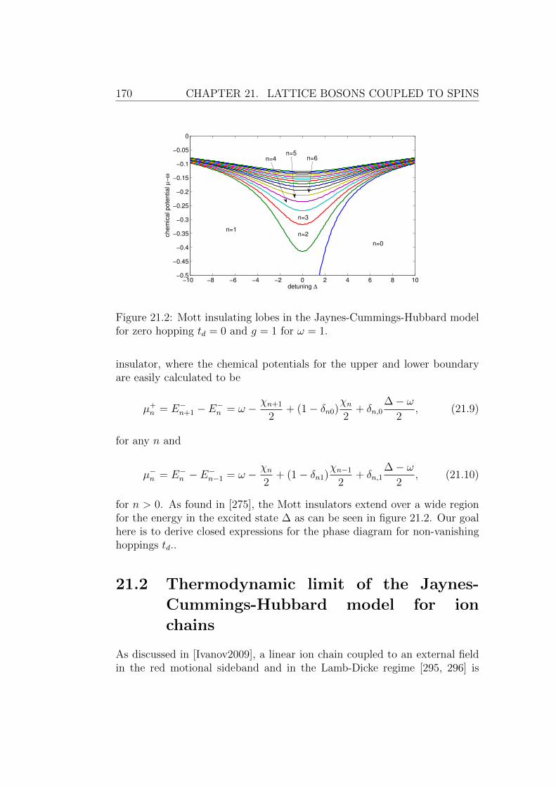
170 CHAPTER 21. LATTICE BOSONS COUPLED TO SPINS
−10 −8 −6 −4 −2 0 2 4 6 8 10−0.5
−0.45
−0.4
−0.35
−0.3
−0.25
−0.2
−0.15
−0.1
−0.05
0
detuning ∆
chem
ical pote
ntial µ
−ω
n=4n=5
n=6
n=0
n=1n=2
n=3
Figure 21.2: Mott insulating lobes in the Jaynes-Cummings-Hubbard modelfor zero hopping td = 0 and g = 1 for ω = 1.
insulator, where the chemical potentials for the upper and lower boundaryare easily calculated to be
µ+n = E−n+1 − E−n = ω − χn+1
2+ (1− δn0)
χn2
+ δn,0∆− ω
2, (21.9)
for any n and
µ−n = E−n − E−n−1 = ω − χn2
+ (1− δn1)χn−1
2+ δn,1
∆− ω2
, (21.10)
for n > 0. As found in [275], the Mott insulators extend over a wide regionfor the energy in the excited state ∆ as can be seen in figure 21.2. Our goalhere is to derive closed expressions for the phase diagram for non-vanishinghoppings td..
21.2 Thermodynamic limit of the Jaynes-
Cummings-Hubbard model for ion
chains
As discussed in [Ivanov2009], a linear ion chain coupled to an external fieldin the red motional sideband and in the Lamb-Dicke regime [295, 296] is

21.2. INFINITE SIZE MODEL FOR ION CHAINS 171
described by the Jaynes-Cummings-Hubbard model, where the hopping cor-responds to phonon transfer through Coulomb interaction. Due to the equi-librium positions of the ion in the harmonic axial potential [297], the bosonicfrequencies and the hopping amplitudes become site-dependent. The fullHamiltonian
H =L−1∑j=0
ωj a†j aj + ∆
∑j
σ†j σ−j + g
∑j
(σ†j aj + a†jσ
−j
)
+L−2∑j=0
L−j−1∑d=1
tj,j+d
(a†j+daj + a†j aj+d
) (21.11)
depends on the number of ions L through the equilibrium positions uj of
the ions which can be determined as shown in [297]. a†j and aj describethe creation and annihilation of a local transversal phonon at the jth site(ion), σ±j are the spin flip operators between the internal states of the ion,∆ is the detuning of the external laser field from the red motional sideband.g describes the phonon-ion coupling in the Lamb-Dicke limit and definesthe energy scale through g = 1; for precise definitions of the quantities see[Ivanov2009]. The local oscillation frequencies ωj and the hopping amplitudestj,j+d are determined by the longitudinal and transversal trap frequencies ωzand ωx via
ωj = − ω2z
2ωx
L−1∑l=0l 6=j
1
|uj − ul|3tj,j+d =
ω2z
2ωx
1
|uj − uj+d|3. (21.12)
For sufficiently large L, the equilibrium positions uj of the ions at the centerare approximately equidistant, giving uj = j u, with u being the distance oftwo adjacent ions. With this, the oscillation frequencies and the hopping am-plitudes (21.12) can be rewritten for L→∞, yielding position independentphonon energies ωj ≡ −ω and hopping amplitudes tj,j+d ≡ td satisfying
td =ω2z
2ωxu3
1
d3= t
1
d3, (21.13)
ω = 2ω2z
2ωxu3ζ(3) = 2t ζ(3), (21.14)
where in the following t = ω2z
2ωxu3acts as a small parameter and ω > 0. ζ(x) is
the Riemann ζ-function. In the expressions (21.13) and (21.14) one noticesa negative oscillator energy −ω and a negative effective mass, which is a

172 CHAPTER 21. LATTICE BOSONS COUPLED TO SPINS
0 0.1 0.2 0.3 0.4 0.5 0.6 0.7 0.8 0.9 110
−10
10−8
10−6
10−4
10−2
100
102
normalized position j
ωj−
ω
L= 10 L= 50 L= 100 L= 500 L=1000
Figure 21.3: Deviation of the finite system phonon energies (21.12) for differ-ent lengths L from the infinite size result (21.14). Beside the larger deviationat the boundaries, the infinite sum gives a good estimate for the finite systemeven for rather small system sizes.
result of the positive hopping strength t which will be of importance later on.
Figure 21.3 shows the accuracy of the assumption of homogeneous phononenergies for different numbers of ions L. Shown is the difference of the exactsummation over the ion positions for a finite chain of length L as found inthe original expression (21.12) for equidistant ions compared to the infinitesize results from (21.14). Beside the larger deviations close to the ends ofthe ion chain, the approximative results are quite satisfying, supporting thevalidity of the homogeneous system assumption in the thermodynamic limit.

CHAPTER 22
Approximative calculation of the phase
diagram
This chapter presents two different approximations for the determination ofthe phase diagram. First, a new approach referred to as fermion approxi-mation is introduced. The second approximation is similar to the strong-coupling expansion common for Hubbard-like Hamiltonians [97] and alreadyapplied to the calculation of the phase diagram of the Jaynes-Cummings-Hubbard model in lower order [276, 277, 280, 284, 283]. We here presentthe full derivation of the second order strong-coupling expansion using theformulation of [97]. Though in [280] a second order treatment is used, theauthors do not discuss the phase diagram but focus on the excitation spec-trum. Recent work presented in [298] applies a field theoretic approach forfinite temperature T to the simple cubic Jaynes-Cummings-Hubbard model.
22.1 Fermion approximation
From (21.7) we note that all terms of the Jaynes-Cummings-Hubbard Hamil-tonian are quadratic. These kinds of models are in general suited for an exactsolution by means of a Fourier transform (9.2). The problem at this pointis however, that the commutation relations of spin operator σ±j are not assimple as that of bosons or fermions. Naively defining the Fourier transformof the spin operators as
σ−k =1√L
∑j
e−2πi kjL σ−j (22.1)
173
174 CHAPTER 22. CALCULATION OF THE PHASE DIAGRAM
destroys the commutator relation for the spins in momentum space:
[σ+k , σ
−k′ ] =
2√Lσzk−k′ 6= 2 σzk δkk′ . (22.2)
Thus, a Fourier transformation of the spins is not useful. The often usedusual trick of a prior Jordan-Wigner transformation [299], transforming thespin operators to fermionic operators, is not applicable in this case, sincethe interaction part is linear in the spin operators, so the Jordan-Wignerfactors do not cancel out. Thus both transformations cannot be carriedout exactly without increasing the descriptional complexity of the problem.Nevertheless the Hamiltonian can be diagonalized by a Fourier-transform inan approximate way introducing fermionic operators.
As noted above, all modes decouple for td = 0. For this reason, the spin-operators are in this limit equivalent to fermionic operators. Assuming the re-placement σ+
j 7→ c†j to hold also for small values of td, the Jaynes-Cummings-Hubbard model (21.7) can be rewritten in a fermionic approximation
H = ω∑j
a†j aj + ∆∑j
c†j cj + g∑j
(c†j aj + a†j cj
)+∑d
td∑j
(a†j aj+d + a†j+daj
).
(22.3)
Within this approximation, a Fourier transform of both, the bosonic andfermionic degrees of freedom can be easily accomplished as defined in (9.2).Doing so, and transforming the momentum-space fermionic operators backto spins, the Jaynes-Cummings-Hubbard Hamiltonian transforms to that ofuncoupled Jaynes-Cummings systems in k-space
H =∑k
ωka†kak + ∆
∑k
σ+k σ−k + g
∑k
(σ+k ak + a†kσ
−k
)(22.4)
with mode dependent phonon energies
ωk = ω + 2∑d
td cos(2πkd
L). (22.5)
The ground state in any mode is given by the Jaynes-Cummings ground state(21.4) with frequency ωk and the energy of mode k with n excitations is
Enk = (1− δn0)
[nωk +
∆− ωk2
− 1
2
√(∆− ωk)2 + 4ng2
]. (22.6)

22.1. FERMION APPROXIMATION 175
Since still the total number of excitations N (in momentum space) in thesystem commutes with the Hamiltonian (22.4), a common basis can bechosen. Thus the full solution of (22.4) for a fixed total number of excitationsN is given by the distribution n = nk1 , nk2 , . . . of N excitations on Lmomentum modes with minimal energy EN [n] =
∑k E
nkk , together with the
constraint∑
k nk ≡ N . Note that the number of momentum modes L isequal to the number of ions (sites).
To construct the phase diagram as usual, the energy for N = nL−1, N = nLand N = nL+ 1 excitations needs to be calculated. In the limit of vanishinghopping (td ≡ 0) and for commensurate filling, i.e., N = nL, the distribu-tion of occupation numbers which has the lowest energy is n = n, n, . . . , n.This corresponds to a Mott-insulating state with an integer number of exci-tations on every lattice site. The phase is gapped with a particle-hole gapas described in chapter 21. When td is increased, the gap slowly closes andeventually a quantum phase transition occurs from the Mott insulator to thesuperfluid phase at some critical value of t. The only remaining task in orderto calculate the chemical potentials is to find the momentum mode where theaddition (removal) of an excitation gives the maximum (minimum) reduction(increase) in the total energy. This yields
µ+n = En+1
k′ − Enk′ µ−n = En
k − En−1k , (22.7)
where k′ [k] is chosen such that µ+n (k′) [µ−n (k)] is minimal [maximal]. The
actual values of k and k′ depend mainly on the sign of the hopping amplitudestd.
Interpretation of the approximation
The transformation used above is not a transformation in the strict sense; ithas to be seen as a valid replacement for td ≡ 0. To understand its validity interms of a proper transformation, we apply a Jordan-Wigner transformation
σ+j = eiπ
∑l<j c
†l cl cj =
∏l<j
(1− 2c†l cl
)cj (22.8)
which connects spin degrees of freedom and fermions. The spins and fermions
are equivalent, if one neglects the phase factor eiπ∑
l<j c†l cl which takes care
of the proper commutation relation within the transformation. This is donein our case as approximative scheme, which ignores effects arising from thecommutator between different sites.

176 CHAPTER 22. CALCULATION OF THE PHASE DIAGRAM
22.2 Strong-coupling
The second, more systematic approximative scheme is a strong-couplingexpansion in the hopping td. This method is well known and determines theenergy of the ground state in a second order perturbative treatment. Havingthe energy as a function of the hopping, the calculation of the chemicalpotentials is straightforward.
a) Initial considerations
For the following discussion it will be useful to consider the action of a singlebosonic creation or annihilation operator on a given (single-site) Jaynes-Cummings eigenstate |±, n〉. This establishes the main influence of the hop-ping operator, since no atomic degrees come up in the perturbation theory.Defining1
A±n =
√n α±n β
−n+1 ±
√n+ 1 β±n α
−n+1 n > 0
α−1 n = 0, (22.9)
B±n =
√n α±n β
+n+1 ∓
√n+ 1 β±n α
+n+1 n > 0
−α+1 n = 0
, (22.10)
C±n =
√n− 1 α±n β
−n−1 ±
√n β±n α
−n−1 n > 1
0 n ≤ 1, (22.11)
D±n =
√n− 1 α±n β
+n−1 ∓
√n β±n α
+n−1 n > 1
±β±1 δn,1 n ≤ 1, (22.12)
the action of a† and a on the state Jaynes-Cummings eigenstate |±, n〉 canbe seen to be
a† |±, n〉 = A±n |+, n+ 1〉+B±n |−, n+ 1〉 (22.13)
a |±, n〉 = C±n |+, n− 1〉+D±n |−, n− 1〉 , (22.14)
i.e., a† and a connect the manifold of states |±, n〉 to the manifolds |±, n+ 1〉and |±, n− 1〉 respectively as expected. As already discussed in chapter 21and figure 21.1, all contributions from the excited Jaynes-Cummings states|+, n〉 can be neglected. This means, that the annihilation (creation) opera-tor on the Jaynes-Cummings ground state acts precisely as the annihilation
1The definition of α±n and β±
n can be found in (21.4).

22.2. STRONG-COUPLING 177
(creation) operator on a number state, i.e., connecting the state |−, n〉 tothe state |−, n± 1〉, together with a prefactor2. This similarity basicallyallows the application of the perturbation theory to the pure Bose-Hubbardmodel with only slight modifications3.
b) Corrections to the energy in second order
In order to calculate the phase boundaries of the Mott insulating lobes forthe Jaynes-Cummings-Hubbard model, we follow the scheme already used inchapter 12. In the following we present a detailed derivation of this scheme.The task is to calculate the energy of the ground state with N excitationsas function of the hoppings td. Here we explicitly discuss the situationof one additional excitation, i.e., N = nL+1, which is the most complex one.
We make again use of Kato’s expansion as presented in [159]. This allows toderive an effective Hamiltonian within the degenerate ground states |Ψ〉jfor the N = nL + 1 manifold, which is L-fold degenerate. Degenerateperturbation theory is straightforward because the hopping processes couplethe different states within the manifold already in first order. The detailedcalculation can be found in appendix C.1. Here we shortly summarize themain steps and results.
The ground-state manifold for N = nL+ 1 excitations is L-fold degenerate,leading to a coupling of all degenerate states via the hopping operator
V =∑d
td∑j
(a†j aj+d + a†j+daj
). (22.15)
This coupling is taken into account by the derivation of an effective Hamil-tonian within the degenerate manifold [159], where the matrix elements ofthe effective Hamiltonian up to second order are defined by
q 〈Ψ| Heff |Ψ〉p =q 〈Ψ| H0 + PV P + PVQ 1
E0 − H0
QV P |Ψ〉p . (22.16)
P projects onto the degenerate manifold, Q = 1 − P and E0 is theground-state energy of the manifold.
2Here, the prefactors are given by B−n and D−
n , whereas the action on a simple numberstate would be given by
√n and
√n+ 1, respectively.
3Replacing the expressions for the energy and the prefactors

178 CHAPTER 22. CALCULATION OF THE PHASE DIAGRAM
The matrix elements of the effective Hamiltonian given in (C.19) show, thatthe additional excitation behaves as a free particle within the manifold. Intro-ducing fermionic operators c†j, cj, which describe the two-dimensional Hilbertspace consisting of the states |1〉 = |−, n+ 1〉 and |0〉 = |−, n〉, the effectivemodel is given by the Hamiltonian
H =∑d
Td∑j
(c†j cj+d + c†j+dcj
)+ ∆
∑j
c†j cj. (22.17)
The local energy ∆ reads
∆ = E−n+1 + 2
(B−n+1D
−nD
−n+2B
−n−1
E−n+1 + E−n − E−n+2 − E−n−1
+(L− 2)B−nD
−nB−n−1D
−n+1
2E−n − E−n−1 − E−n+1
)∑d
t2d
(22.18)
and the modified hopping constants Td are
Td = B−nD−n+1td +
B−nD−nB−n−1D
−n+1
2E−n − E−n−1 − E−n+1
Td (22.19)
with Td (which is of order t2d) given in (C.18).
The solution of the effective fermion Hamiltonian in (22.17) is straightfor-ward. Applying a Fourier transformation (9.2) to the Hamiltonian gives
H =∑k
[∆ + 2
∑d
Td cos
(2πkd
L
)]c†kck =
∑k
Ωk c†kck. (22.20)
The ground state for the single additional excitation case is equivalent tothe determination of the minimum in the dispersion relation Ωk. Thus,the energy in second order of the hopping amplitudes for the additionalexcitation state is given by E(N = nL + 1) = Ωq, where q has to bedetermined from the dispersion. If all td are of the same sign, the minimumis easy to find, where for td < 0 the mode q = 0 gives the minimum and fortd > 0 the minimum is found for q = L/2. In all intermediate situations, i.e.,if the td have different signs, the situation has to be analyzed more carefully.This result generalizes the findings from [277, 280] to arbitrary hoppings td.
A similar treatment finally allows to calculate the energy of the Mott insula-tor as well as for the system with one excitation less. The slightly deviatingexpressions for ∆ and Td are not given explicitly here, however. From theseenergies, the chemical potentials are defined as usually, giving the boundaryof the Mott insulator through µ±n = ±E(nL± 1)∓ E(nL).

22.3. MEAN-FIELD THEORY 179
22.3 Mean-field theory
The simplest numerical method to obtain a qualitative phase diagram isthe so-called mean-field theory. As described for instance in [181, 272, 275,292, 300], a mean-field theory can be implemented by introducing an orderparameter Ψ, which in our case is chosen to be homogeneous and real valued.Decoupling the hopping term by using
a†j al 7→ Ψ(a†j + al
)− |Ψ|2 , (22.21)
the Jaynes-Cummings-Hubbard Hamiltonian (21.7) in the grand-canonicalensemble uncouples in real space to a local Hamiltonian
HMF = (ω − µ) a†a+ (∆− µ) σ+σ− + g(a†σ− + aσ+
)− 2JΨ
(a† + a
)+ 2J |Ψ|2 . (22.22)
At this point, we omitted the spatial index because the problem is purelylocal. The modified hopping amplitude J = −
∑d td gives the effective cou-
pling within the mean-field scheme. The phase diagram is now found bydiagonalizing the mean-field Hamiltonian (22.22) either exactly by meansof perturbation theory [181] or numerically, setting an upper bound for themaximal number of bosonic excitations in the system. The ground-state en-ergy is then given by minΨE[Ψ] and the Mott insulator is distinguished fromthe superfluid by the value of Ψ for the minimal energy. For Ψ ≡ 0, the sys-tem is in a Mott insulating state, for Ψ > 0, the ground state is superfluid.This sets the point of the Mott-insulator to superfluid transition. It shouldbe mentioned at this point, that this method gives inadequate results in onedimension (D = 1) but is exact for D → ∞. Additionally, the effective
hopping J must be larger than zero to yield any result.

CHAPTER 23
Benchmarking against the
Jaynes-Cummings-Hubbard model with
nearest-neighbor hopping
In this chapter, we benchmark the newly introduced fermion approximationon the simple cubic Jaynes-Cummings-Hubbard model with nearest-neighborhopping td = −tδd1. This is the natural choice, since for this variant of themodel, well established numerical results from DMRG calculations [278] aswell as earlier (perturbative) analytic results exist. Furthermore, the resultsof the introduced mean-field theory are well understood in this case.
The simple cubic Jaynes-Cummings-Hubbard model with nearest-neighborhopping is given by
H = ω∑j
a†j aj + ∆∑j
σ†j σ−j + g
∑j
(σ†j aj + a†jσ
−j
)− t∑j
(a†j aj+1 + a†j+1aj
),
(23.1)
where we focus on the resonant case, i.e., ω = ∆.
23.1 Strong-coupling results
To calculate the chemical potentials using the strong-coupling approximation,we first have to determine the momentum mode q and q′ which minimizesthe energy (22.20). Since td < 0 for any distance d, this is found for q = 0.
181

182 CHAPTER 23. BENCHMARKING AGAINST NN-JCHM
Furthermore, the coefficients in (21.4) are α±n = 1√2
= β±n and therefore
B−n =
√n+√n+1
2n > 0
− 1√2
n = 0
= D−n+1. (23.2)
This allows for a conclusive calculation of the chemical potentials which arenot shown here. Nevertheless, we give the approximative results for the tipof the lobe in the first order perturbation theory. The chemical potentialsare found to be
µ+n = ω − 1
2χn+1 +
1− δn0
2χn − t
(√n+√n+ 1
)2
2− δn0
, (23.3)
for any n and
µ−n = ω − 1
2χn +
1− δn1
2χn−1 + t
(√n+√n− 1
)2
2− δn1
, (23.4)
for n > 0, which gives the tip of the Mott lobe, defined by µ+n = µ−n to be
tcrit/g = 22√n−√n+ 1−
√n− 1
(√n+√n+ 1)2 + (
√n+ δn1 +
√n− 1)2
. (23.5)
A comparison of these results to the numerical results from DMRG is givenin figure 23.1
23.2 Fermion approximation
Secondly we apply the fermion approximation to this model. With the givensystem parameters, the momentum dependent phonon energies (22.5) areωk = ω − 2t cos(2π k
L) and the energy (22.6) in the kth momentum mode for
a given filling n reads
Enk = (1− δn0)
[nω − 2n t cos(2π
k
L) + t cos(2π
k
L)−
√t2 cos2(2π
k
L) + ng2
].
(23.6)Finally, following (22.7), the momentum modes k′ (k) which minimize (max-imize) the chemical potentials need to be found. In the present case (t1 < 0),these are k′ = 0 and k = L
2. Thus the resulting chemical potentials are
µ+n − ω = −2t+ tδn0 −
√t2 + (n+ 1)g2 + (1− δn0)
√t2 + ng2, (23.7)
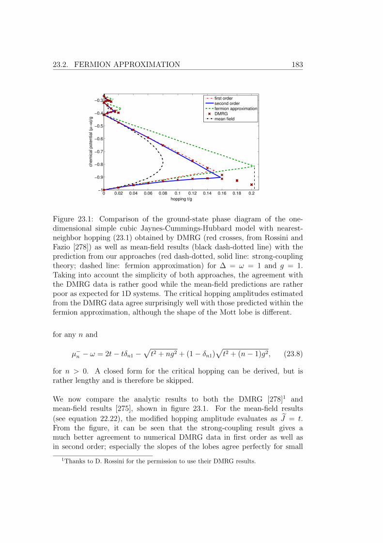
23.2. FERMION APPROXIMATION 183
0 0.02 0.04 0.06 0.08 0.1 0.12 0.14 0.16 0.18 0.2−1
−0.9
−0.8
−0.7
−0.6
−0.5
−0.4
−0.3
chem
ical pote
ntial (µ
−ω
)/g
hopping t/g
first ordersecond orderfermion approximationDMRGmean field
Figure 23.1: Comparison of the ground-state phase diagram of the one-dimensional simple cubic Jaynes-Cummings-Hubbard model with nearest-neighbor hopping (23.1) obtained by DMRG (red crosses, from Rossini andFazio [278]) as well as mean-field results (black dash-dotted line) with theprediction from our approaches (red dash-dotted, solid line: strong-couplingtheory; dashed line: fermion approximation) for ∆ = ω = 1 and g = 1.Taking into account the simplicity of both approaches, the agreement withthe DMRG data is rather good while the mean-field predictions are ratherpoor as expected for 1D systems. The critical hopping amplitudes estimatedfrom the DMRG data agree surprisingly well with those predicted within thefermion approximation, although the shape of the Mott lobe is different.
for any n and
µ−n − ω = 2t− tδn1 −√t2 + ng2 + (1− δn1)
√t2 + (n− 1)g2, (23.8)
for n > 0. A closed form for the critical hopping can be derived, but israther lengthy and is therefore be skipped.
We now compare the analytic results to both the DMRG [278]1 andmean-field results [275], shown in figure 23.1. For the mean-field results
(see equation 22.22), the modified hopping amplitude evaluates as J = t.From the figure, it can be seen that the strong-coupling result gives amuch better agreement to numerical DMRG data in first order as well asin second order; especially the slopes of the lobes agree perfectly for small
1Thanks to D. Rossini for the permission to use their DMRG results.
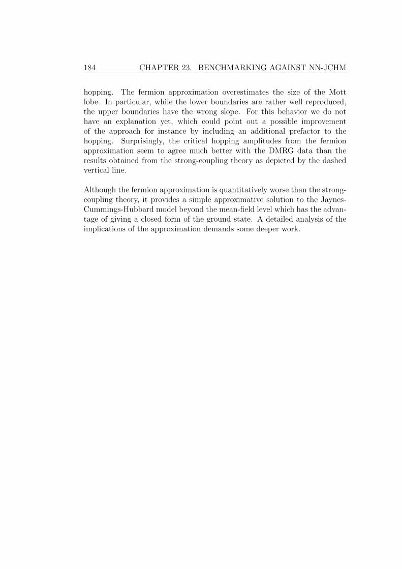
184 CHAPTER 23. BENCHMARKING AGAINST NN-JCHM
hopping. The fermion approximation overestimates the size of the Mottlobe. In particular, while the lower boundaries are rather well reproduced,the upper boundaries have the wrong slope. For this behavior we do nothave an explanation yet, which could point out a possible improvementof the approach for instance by including an additional prefactor to thehopping. Surprisingly, the critical hopping amplitudes from the fermionapproximation seem to agree much better with the DMRG data than theresults obtained from the strong-coupling theory as depicted by the dashedvertical line.
Although the fermion approximation is quantitatively worse than the strong-coupling theory, it provides a simple approximative solution to the Jaynes-Cummings-Hubbard model beyond the mean-field level which has the advan-tage of giving a closed form of the ground state. A detailed analysis of theimplications of the approximation demands some deeper work.
CHAPTER 24
Application to the ion-chain setup
The first thing to notice in the Hamiltonian for the ion-chain setup in thethermodynamic limit is the negative oscillator energy ωj = −ω < 0 (21.14)as well as the negative effective mass td = t 1
d3> 0 (21.13). This nega-
tive mass is the reason why the application of the mean-field theory is notthat straightforward. Simply calculating the modified hopping amplitudeJ = −t
∑d
1d3
= −tζ(3) as defined in section 22.3, the hopping becomes neg-ative and therefore mean-field theory is inapplicable. This problem can beovercome by first applying a canonical transformation to all used operators.The transformation
aj 7→ (−1)j aj (24.1)
for the annihilation operator and accordingly to all the other operatorsa†j,σ
±j , maps the Jaynes-Cummings-Hubbard model (21.7) onto itself, but
with td 7→ (−1)dtd. After this transformation, the modified hopping evalu-
ates to J = −t∑
d(−1)d
d3= 3tζ(3)/4, being positive. Now the application of
the mean-field theory is straightforward, following the usual route.
Starting with the effective strong-coupling theory described in detail insection C.1, the chemical potentials for the upper and lower boundary of thelobes can be calculated. The proper momentum modes q, q′, which minimize(maximize) the chemical potentials are both found to be q = q′ = L/2,which results from the negative mass. Due to the complexity of the problem,especially the analytic form of B−n and D−n , analytic expressions of thechemical potentials are omitted. Up to second order, the results for thephase diagram are shown in figure 24.3, together with a comparison to themean-field results and the fermion approximation.
185

186 CHAPTER 24. APPLICATION TO THE ION-CHAIN SETUP
0 0.1 0.2 0.3 0.4 0.5 0.6 0.7 0.8 0.9 1
−5
−4.5
−4
−3.5
−3
−2.5
−2
−1.5
−1
−0.5
0
sin
gle
part
icle
energ
y E
n k [g]
momentum k/L
n=0
n=1
n=2
n=3
n=4
Figure 24.1: Energies of the Jaynes-Cummings-Hubbard Hamiltonian in mo-mentum space after application of the fermion approximation for fixed fillingn. Shown are the energies (22.6) for the five lowest fillings 0 . . . 4 (from topto bottom) for ∆ = 0 and g = 1. Solid lines: t/g = 0.02; Dash-dotted lines:t/g = 0.2. One clearly recognizes the minimum at k = L/2 and the flatdispersion for t/g → 0.
Following the approximative method from section 22.1, the Hamiltonian forthe uncoupled Jaynes-Cummings models is given by (22.4), with the phononenergies
ωk = −ω + 2t∑d
cos(2π kdL
)
d3, (24.2)
according to (22.5). Note that since ω = 2t ζ(3), all ωk’s are negative. Using
the polylogarithm Lin (x) =∑∞
d=1xd
dnthey can be written explicitly as
ωk = t[Li3
(e2πi k
L
)+ Li3
(e−2πi k
L
)− 2ζ(3)
]. (24.3)
The minimum value of ωk = −7tζ(3)/2 is attained for k = L2
as expectedfrom the positive sign of the hopping term. The energies for each momentummode are given by the solution (22.6) of the Jaynes-Cummings model and thecorresponding spectrum is shown in figure 24.1. Note the minimum at k = L
2.
From the dispersion relation for different fillings, it is now easy to constructthe phase diagram. As discussed in section 22.1, the flat dispersion for t = 0
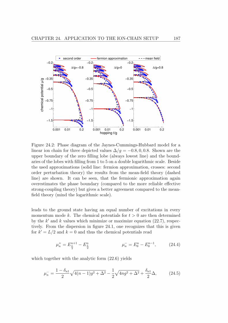
CHAPTER 24. APPLICATION TO THE ION-CHAIN SETUP 187
0.001 0.01 0.2
−1.5
−1
−0.75
−0.5
−0.35
−0.2
ch
em
ica
l p
ote
ntia
l µ
/g
0.001 0.01 0.2
−1.5
−1
−0.75
−0.5
−0.35
−0.2
hopping t/g
0.001 0.01 0.2
−1.5
−1
−0.75
−0.5
−0.35
−0.2
second order fermion approximation mean field
∆/g=0.8∆/g=0∆/g=−0.8
Figure 24.2: Phase diagram of the Jaynes-Cummings-Hubbard model for alinear ion chain for three depicted values ∆/g = −0.8, 0, 0.8. Shown are theupper boundary of the zero filling lobe (always lowest line) and the bound-aries of the lobes with filling from 1 to 5 on a double logarithmic scale. Besidethe used approximations (solid line: fermion approximation, crosses: secondorder perturbation theory) the results from the mean-field theory (dashedline) are shown. It can be seen, that the fermionic approximation againoverestimates the phase boundary (compared to the more reliable effectivestrong-coupling theory) but gives a better agreement compared to the mean-field theory (mind the logarithmic scale).
leads to the ground state having an equal number of excitations in everymomentum mode k. The chemical potentials for t > 0 are then determinedby the k′ and k values which minimize or maximize equation (22.7), respec-tively. From the dispersion in figure 24.1, one recognizes that this is givenfor k′ = L/2 and k = 0 and thus the chemical potentials read
µ+n = En+1
L2
− EnL2
µ−n = En0 − En−1
0 , (24.4)
which together with the analytic form (22.6) yields
µ−n =1− δn1
2
√4(n− 1)g2 + ∆2 − 1
2
√4ng2 + ∆2 +
δn1
2∆, (24.5)

188 CHAPTER 24. APPLICATION TO THE ION-CHAIN SETUP
Figure 24.3: Phase diagram of the Jaynes-Cummings-Hubbard model for alinear ion chain from the fermion approximation. Boundaries of the Mottlobes (from bottom to top) for n = 2, 3, 4. The lobes n = 0 and n = 1 arenot displayed since they are unbounded for ∆→ −∞.
and
µ+n =
1
2
[−
√4(n+ 1)g2 +
(7
2ζ(3)t+ ∆
)2
− 7
1 + δn0
ζ(3)t+ δn0∆
+ (1− δn0)
√4ng2 + (
7
2ζ(3)t+ ∆)2
]. (24.6)
This allows to determine the resulting phase diagram shown in figure 24.2for three values of ∆ comparing the different approaches. One recognizesthe typical lobe structure of the Mott insulator phases with a closing of thelobes at some value tcrit
n (∆). While the mean-field results underestimate theextent of the Mott insulating regions greatly (note the logarithmic scale), thefermionic approach overestimates them but with a better agreement to thestrong-coupling theory than the mean-field solution. The main advantage ofthe fermionic approximation is the closed form for the chemical potentials forthe ground state. Figure 24.3 shows the full phase diagram of the model asa function of the detuning ∆ obtained from the fermionic approximation only.
The critical hopping amplitude tcritn (∆) can be calculated from the analytic
expressions for the chemical potential given above. Figure 24.4 showsthe dependence of the critical hopping amplitude on the detuning ∆ for

CHAPTER 24. APPLICATION TO THE ION-CHAIN SETUP 189
−5 0 5
10−3
10−2
10−1
100
detuning ∆/g
critical hoppin
g t
nCrit /g
n=1n=2n=3n=4n=5n=6n=7n=8pert. theo.
Figure 24.4: Critical hopping amplitude tcritn (∆) which gives the point where
the Mott-insulator to superfluid transition takes place. From top to bottom:n = 1 . . . 8, all for g=0.05. The crosses present the results for the strong-coupling theory whereas the solid lines are the results from the fermionicapproximation.
the different Mott lobes. Note the unboundedness of the first lobe, i.e.,tcritn (∆) → ∞ as ∆ → −∞. Additionally, the figure shows the critical
hopping calculated from the strong-coupling theory for the first lobe givinga reasonable agreement of both methods.

CHAPTER 25
Conclusion and outlook
Approximating the spin-degrees of freedom in the Jaynes-Cummings-Hubbard model as fermions results in an easy analytic solution of theHamiltonian, yielding closed expressions for the phase diagram. Althoughthe used approximation is not fully understood yet, the predictions basedon it give quite reasonable results compared to DMRG or strong-couplingtheory. Being applicable to arbitrary long-ranged hopping, we constructedthe phase diagram for a system describing ions in a linear ion chain. Thissolution of allows for an easy estimate of the position of the phase transition,not available from other methods, yet.
Though providing reasonable results, the used fermionic approximation lackssome important features. The missing understanding limits its trustworthi-ness where further extensions of the approximation should improve the re-sults compared to perturbation theory, especially for the upper boundariesof the Mott insulators. Nevertheless, applications to the dynamics in theJaynes-Cummings-Hubbard model or extensions thereof such as the spin-boson model will provide a deeper understanding of the model as well asfurther benchmarks of the approximation.
191


Appendix
193

APPENDIX A
Ultrafast Fermions
A.1 Fourier transform of the coupling con-
stants
As discussed in section 9.3 in part II, the Fourier transform of the couplings(9.12) is governed by the Fourier transform of the numerator. At this placewe will prove the result given in the main text using the Poisson sum formula[301]
∞∑d=−∞
f(d) =∞∑
l=−∞
∞∫−∞
f(x)e−2πilxdx. (A.1)
Using the definition of the Fourier transform (9.18) together with a rewritingof the cosine parts, the Fourier transformation can be written as
∞∑d=−∞
cos dξ cos dξ′eikd =1
4
∑C1,C2=−1,1
∞∑d=−∞
eid(C1ξ+C2ξ′+k) (A.2)
:=1
4
∑C1,C2=−1,1
∞∑d=−∞
eidα. (A.3)
For the last term, we now apply the Poisson sum formula:
∞∑d=−∞
eiαd =∞∑
l=−∞
∞∫−∞
eixαe−2πilxdx (A.4)
195
196 APPENDIX A. ULTRAFAST FERMIONS
=∞∑
l=−∞
∞∫−∞
ei(α−2πl)xdx (A.5)
= 2π∞∑
l=−∞
δ(α− 2πl). (A.6)
Together with the definition of α we end up in the stated relation
∞∑d=−∞
cos dξ cos dξ′eikd =π
2
∞∑l=−∞
∑C1,C2=−1,1
δ(2πl − C1ξ − C2ξ′ − k). (A.7)
A.2 Fourier transform of the Green’s func-
tions
In section 10.2, the solution of the Dyson equation for the Green’s functionis presented. At this point we summarize the important points in the Fouriertransform of the Green’s functions, going back from the frequency domainto time domain. From equations (10.15) and (10.16) and with the definitionof the Fourier transform
G(±)kk′ (t+ T, t) =
1√2π
∞∫−∞
dω G(±)kk′ (ω)eiωT , (A.8)
the calculation of G(±)kk′ (t+ T, t) is straight forward.
a) Equal momentum
For G(±)kk (t+ T, t), the Fourier transformation together with (10.15) gives
G(±)kk (t+ T, t) = ± i
2π
∞∫−∞
dωεk ± ω ⊕ iδ
ε2k ⊕ 2iδεk − δ2 − ω2 +
V 2η2B%2B
~2
eiωT . (A.9)
Since the convergence factor δ is chosen in the limit δ → 0, the δ2 in thedenominator may be neglected. Looking at the dispersion of the free fermions(10.9) and taking into account the definition of ⊕, the combination ⊕εk isalways of negative sign, since for k ∈ KF , ⊕ means + but εk < 0. In the
A.3. ZERO-HOPPING ENERGIES FOR THE PHASE DIAGRAM 197
other case the signs are just the other way around. Neglecting the factor of2 before the δ and defining the renormalized dispersion
εk =
√ε2k +
V 2η2Bη
2B
~2, (A.10)
the Green’s function calculates as
G(±)kk (t+ T, t) = ± i
2π
∞∫−∞
dωεk ± ω ⊕ iδε2k − ω2 − iδ
eiωT . (A.11)
This integration is done by means of residue integration [302], where the con-tour is closed in the upper half plain, enclosing the pole at ω0 = −
√ε2k − iδ.
Finally, after performing the limit δ → 0, the Green’s function is given by
G(±)kk (t+ T, t) =
1
2e−iεkT
(1∓ εk
εk
). (A.12)
b) Unequal momentum
The calculation for G(±)
kk+L2
(t+T, t) follows the same route as described above.
Using the result for the Green’s function in the frequency domain (10.16) andthe same argument for the combination ⊕εk as above, the Fourier transformis calculated from
G(±)
k±L2k(t+ T, t) = i
V ηB%B2π~
∞∫−∞
dω1
ε2k − ω2 − iδ
eiωT . (A.13)
Again closing the contour in the upper half plain with the same pole as above,the residue integration gives
G(±)
k±L2k(t+ T, t) = −V ηB%B
2~1
εke−iεkT (A.14)
as stated in the main text.
A.3 Zero-hopping energies for the phase dia-
gram
Chapter 12 shows, how to calculate the phase diagram of the effective bosonicHamiltonian analytically. Here we present exemplary the calculation of theenergies for the three different incompressible phases.
198 APPENDIX A. ULTRAFAST FERMIONS
a) CDW phase %B = 12
As discussed in the main text, the ground state for precisely half filling isgiven by the distribution
• • ‖ • ‖ • • ∧= nj = nj =
1
2
[1 + (−1)j
]. (A.15)
Adding a single particle results in the two possible situation, where the ad-ditional particle goes to a double occupation at an even site or to an odd sitehaving only single occupations.
i) Double occupation
In the case for the double occupation, the boson distribution is written as
• • ‖ •• ‖ • • ⇒ nj = nj + δj,0. (A.16)
Plugging this into the effective Hamiltonian (12.1), the energy may be cal-culated straightforwardly.
E[• • ‖ •• ‖ • •]
=U
2
∑j
(nj + δj,0) (nj + δj,0 − 1)− µ∑j
(nj + δj,0) (A.17)
−∆∑j
(nj + δj,0)(−1)j +∑j
∑d
gd(a)(nj + δj,0)(nj+d + δj+d,0)
=U
2
∑j
[2njδj,0 + δ2
j,0 − δj,0]− µ−∆
+∑j
∑d
gd(a) [njδj+d,0 + nj+dδj,0 + δj,0δj+d,0] (A.18)
− µ∑j
nj −∆∑j
nj(−1)j +∑j
∑d
gd(a)njnj+d
= E[• • ‖ • ‖ • •] (A.19)
+ U − µ−∆ +1
2
∑d
gd(a)(1 + (−1)d
)+ g0(a)
= E[• • ‖ • ‖ • •] (A.20)
+ U − µ−∆ + ga(0) + ga(π) + g0(a).
A.3. ZERO-HOPPING ENERGIES FOR THE PHASE DIAGRAM 199
ii) Single occupation
For the single occupation, the calculation of the energy follows exactly thesame route. The boson occupation may be written as
• • ‖ • ‖ • • • ⇒ nj = nj + δj,1 (A.21)
and the energy gives:
E[• • ‖ • ‖ • • •]
=U
2
∑j
(nj + δj,1) (nj + δj,1 − 1)− µ∑j
(nj + δj,1) (A.22)
−∆∑j
(nj + δj,1)(−1)j +∑j
∑d
gd(a)(nj + δj,1)(nj+d + δj+d,1)
=U
2
∑j
[2njδj,1 + δ2
j,1 − δj,1]− µ+ ∆
+∑j
∑d
gd(a) [njδj+d,1 + nj+dδj,1 + δj,1δj+d,1] (A.23)
− µ∑j
nj −∆∑j
nj(−1)j +∑j
∑d
gd(a)njnj+d
= E[• • ‖ • ‖ • •] (A.24)
− µ+ ∆ +1
2
∑d
gd(a)(1− (−1)d
)+ g0(a)
= E[• • ‖ • ‖ • •]− µ+ ∆ + ga(0)− ga(π) + g0(a). (A.25)
b) Mott insulator %B = 1
Now, for ηB ≡ 0, the calculation of the energy for the addition or removal ofa single particle is straightforward. The states themselves are given by
• • • • ‖ •• ‖ • • • • ⇒ nj = 1 + δj,0 (A.26)
and
• • • • ‖ ‖ • • • • ⇒ nj = 1− δj,0. (A.27)
200 APPENDIX A. ULTRAFAST FERMIONS
Using the effective Hamiltonian (10.39) for ηB ≡ 0 we can calculate theenergy for both configurations at once. This gives
E(L± 1) = ±U2
∑j
(1± δj,0)δj,0 − µ∑j
(1± δj,0) (A.28)
−∆∑j
(−1)j(1± δj,0) +∑j
∑d
gd(0)(1± δj,0)(1± δj+D,0)
= ±U2
(1± 1)− Lµ∓ µ∓∆ (A.29)
+∑j
∑d
gd(0) [1± δj+D,0 ± δj,0 + δj,0δj+D,0]
= E(L) +U
2(1± 1)∓ µ∓∆± 2g0(0) + g0(0). (A.30)
A.4 Green’s function approach to spinless
fermions in an alternating potential
Chapter 10 provides a renormalization procedure for the case of double halffilling of the fermions and bosons. In this chapter we generalize these resultsto arbitrary fillings of the form %F = 1
m, where m ∈ N and %B = %F . As
already discussed in chapter 9, the fermions trigger a bosonic CDW at thesame density, where the term CDW for m > 2 is not that accurate. Forinstance for m = 4, i.e., %F = %B = 1
4, the bosonic distribution according to
the induced couplings is given by the case where a boson is found in everyfourth site. So as a starting point for the renormalization of the fermionicsystem, the potential influencing the fermions is that of a potential with asingular peak in every fourth site. For general m, the fermionic problem isthus given by the bosonic mean-field amplitude
nj = %B(1− ηB) +m%BηB δ(sin(πj
m)), (A.31)
as introduced in chapter 10 and together with this, the fermionic Hamiltonianfrom (8.3) looks like
HF = −JF∑j
(c†j cj+1 + c†j+1cj
)+ V m
∑j
δ(sin(πj
m))c†j cj. (A.32)
Here we replaced the factor V ηB%B by V since our result is more generalthan only renormalizing the coupling constants as a function of ηB. Again,

A.4. SPINLESS FERMIONS IN AN ALTERNATING POTENTIAL 201
m=3
m=4
m=2
V
Figure A.1: Visualization of the Dirac comb potential for different periodsm.
the constant energy %F%B(1 − ηB) is neglected and in the following we willrefer to this model as to free fermions in a Dirac comb potential. Figure A.1visualizes the underlying potential in this problem for different values of m.
In the direct solution for the case m = 2 we switched into momentum spacesince this turned out to be much simpler. This still holds for the general-ized Hamiltonian (A.32) which in momentum space, after application of theFourier transform (9.2) is given by
HF =
L/2−1∑k=−L/2
εk f†k fk + V
m−1∑α=−(m−1)
α 6=0
L/2−1∑k=−L/2
f †k+ L
mαfk, . (A.33)
The summation over α is restricted because of the limitation in the possiblemomentum modes k ∈ [−L
2, L
2−1] and the α = 0 term is neglected because it
would only give a constant energy. The single particle energies are given byεk = −2JF cos(2π k
L). This Hamiltonian is the starting point for the calcula-
tion of the Green’s function as already done in chapter 10. But before usingthe perturbative treatment, we discuss the possibility of a direct solution ofthe real space version (A.32) of the model.
a) Exact solution via canonical transformation
The considered Hamiltonian (A.32) is quadratic in the creation and anni-hilation operators and can be solved analytically by means of a canonicaltransformation. This can be easily seen after rewriting the Hamiltonian such

202 APPENDIX A. ULTRAFAST FERMIONS
that the quadratic structure becomes obvious:
H =∑l
c †l
0 −JF−JF V −JF
−JF 0 −JF. . . . . . . . .
−JF 0
cl. (A.34)
Here cl = (clm−1, clm, clm+1, . . . , clm+m−1)T. The transformation can now befound by diagonalizing the matrix ¯M = [· · · ] = U †DU from above Hamilto-nian and defining new fermionic operators el = U cl (a similar approach ispresented in [178, 234]). The diagonalized Hamiltonian is then given by
H =∑l
m−1∑n=−1
εn+2 e†lm+nelm+n =
∑j
εj e†j ej, (A.35)
where εp is the p−th eigenvalues of ¯M and the on-site energies εj are definedas
εj =
ε1 + εm+1 rem(j,m) = m− 1
εrem(j,m)+2 else. (A.36)
rem(j,m) is the remainder after division of j by m.
Since for any m the system is periodic, the single particle energies εj haveperiod m, too and are typically non-degenerate. The solution of this Hamil-tonian for a fixed fermionic density
%F =∑j
c†j cj =∑j
e†j ej (A.37)
is straightforward. Defining the set J of minimal single particle energies
J = j ∈ Z∣∣εj = min
p=0...m−1εp, (A.38)
the ground state of Hamiltonian (A.35) manifold is given by any possiblecombination of particles located at sites, where only sites from J are occu-pied. For the typical case of a unique minimal value εj and a finite lattice oflength L, the cardinality of the set J is equal to %FL and the ground stateis given by
|Ψ〉 =∏j∈J
e†j |0〉 . (A.39)

A.4. SPINLESS FERMIONS IN AN ALTERNATING POTENTIAL 203
Although this solution of Hamiltonian (A.32) using the canonical transforma-tion is straightforward, the resulting ground state is nontrivial and thereforethe transformation back to the original system will not be done. Insteadwe will apply a Green’s functions approach for the calculation of differentexpectation values of the ground state of Hamiltonian (A.33).
b) Green’s functions approach
So far, the derivation of the Dyson equation for the Green’s function doesnot strongly differ from the results already presented in section 10.1. Theonly difference is given by the different range of the sum over α (compare theHamiltonian (A.32) to the m = 2 Hamiltonian from (10.5)). This leads, re-
stricting our discussion to the case of the advanced Green’s function G(+)k,k′(ω),
to the Dyson equation
G(+)k,k′(ω) = G(0+)
k,k′ (ω) +i
~√
2πV G(0+)k,k (ω)
m−1∑α=−m+1α 6=0
G(+)
k+ Lmα,k′
(ω) (A.40)
in both momentum and frequency space. This Dyson equation allows for astraightforward solution in the case m = 2 as presented in chapter 10 withmore difficulties for other m. Nevertheless, a full algebraic solution may befound. Recognizing that above Dyson equation may be rewritten in the form
G(0+)kk′ (ω) =
m−1∑α=−(m−1)
Γk,α G(+)
k+ Lmα,k′
(ω) (A.41)
and that according to the properties of the unperturbed Green’s functionG(0+)k,k′ ∼ δk,k′ only the contributions of the form G(+)
k+p Lm,k′
are non-zero, all
Dyson equations for the non-zero elements may be put into matrix form:
G(0+)
k+m−1m
L,k′(ω)
G(0+)
k+m−2m
L,k′(ω)
...
G(0+)k,k′ (ω)
...
G(0+)
k−m−2m
L,k′(ω)
G(0+)
k−m−1m
L,k′(ω)
= ¯Γ
G(+)
k+m−1m
L,k′(ω)
G(+)
k+m−2m
L,k′(ω)
...
G(+)k,k′(ω)
...
G(+)
k−m−2m
L,k′(ω)
G(+)
k−m−1m
L,k′(ω)
(A.42)

204 APPENDIX A. ULTRAFAST FERMIONS
with
¯Γ =
1 Γm−1m
Γm−1m
. . . 0 0 0
Γm−2m
1 Γm−2m
. . . Γm−2m
0 0...
. . ....
Γ0 Γ0 . . . 1 . . . Γ0 Γ0...
. . ....
...
0 0 Γ−m−2m
. . . Γ−m−2m
1 Γ−m−2m
0 0 0 . . . Γ−m−1m
Γ−m−1m
1
. (A.43)
Here Γβ = Γk+βL,1 and Γk,α = δα0−(1−δα0) i~√
2πV G(0+)k,k simplify the writing.
This matrix equation can be solved for G(+)k,k′ by inverting the matrix ¯Γ and
considering the proper entries. All further results rely on this procedure,where the remaining task in the solution is not the inversion of the matrix¯Γ which is (only) of size (2m − 1) × (2m − 1), but the following Fouriertransformation of the Green’s function into time domain. For m = 2 thismay be done easily whereas for larger m numerical residue integrationturns out to be more suitable. Together with the numerical evaluation ofthe Fourier transform, this now allows for the calculation of the real spaceGreen’s functions and the expectation values of the system from these.
c) Expectation values
Above algebraic equation allows for the calculation of the Green’s functionG(+)k,k′(ω) which is directly connected to all needed expectation values. The real
space Green’s function connects to the momentum space Green’s functionsas
G(+)j,j+d(ω) =
1
L
L/2−1∑k1,k2=−L/2
e−2πi(k1−k2)
Lje−2πi
k1LdG(+)
k2,k1(ω). (A.44)
Again, the summation over the second index is limited because of the prop-erties of the Green’s function, in general incorporated by including the term
m−1∑n=−(m−1)
δk1+ nmL,k2 (A.45)
to the summation. This results in
G(+)j,j+d(ω) =
1
L
∑k
m−1∑n=−m+1
e−2πi kLde−2πi n
mjG(+)
k1+ nmL,k1
(ω) (A.46)
A.4. SPINLESS FERMIONS IN AN ALTERNATING POTENTIAL 205
which together with
G(±)j,j+d(t+ T, t) =
1√2π
∞∫−∞
dω G(±)j,j+d(ω)eiωT (A.47)
at the end gives the final expression for the calculation of the expectationvalues.

APPENDIX B
Multi-band physics
B.1 Calculation of the second order cumulant
We present the derivation of the effective first-band Hamiltonian from thescattering matrix in (16.5) together with the full interaction Hamiltonian. Inthe reduced scattering matrix of the multi-band Bose-Fermi-Hubbard model,the second order cumulant
〈〈T HI(τ + T )HI(τ)〉〉bth (B.1)
in the interaction picture needs to be calculated with respect to the vacuumin the b-th band. Because of the average over the vacuum, the evaluation ofthe cumulant simplifies considerably. For instance, from the last interactionHamiltonian at time τ , only those terms with no annihilation operators inthe b-th band contribute. This strongly reduces the computational effort.For a detailed analysis, we first rewrite the interaction Hamiltonian HI(σ)in such a way, that the occurring contributions become apparent. Omittingthe explicit time dependence σ, the Hamiltonian in the interaction picture isgiven by
H intbth =
∑j
Ubb11
2
(a†b,j
)2
a21,j
::::::::::::::::::À
+Ubb11
2
(a†1,j
)2
a2b,j
À
+ 4Ubb11
2nb,jn1,j
+Vbb11
2a†b,j c
†b,j c1,j a1,j
:::::::::::::::::::Á
+Vbb11
2a†1,j c
†1,j cb,j ab,j
Á
+Vb11b
2m1,jnb,j
(B.2)
207
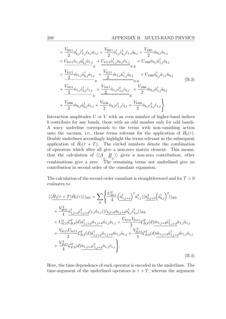
208 APPENDIX B. MULTI-BAND PHYSICS
+Vbb11
2a†b,j c
†1,j cb,j a1,j +
Vbb11
2a†1,j c
†b,j c1,j ab,j +
V1bb1
2mb,jn1,j
+ Ub111n1,j a†b,j a1,j
::::::::::::::::Â
+ Ub111a†1,j ab,jn1,j
Â,Ã
+ U1bbbnb,j a†1,j ab,j
+Vb111
2m1,j a
†b,j a1,j
:::::::::::::::::Ã
+Vb111
2m1,j a
†1,j ab,j
Â,Ã
+ U1bbba†b,j a1,jnb,j
+V1b11
2n1,j c
†b,j c1,j
::::::::::::::::Ä
+V1b11
2n1,j c
†1,j cb,j
Ä
+V1bbb
2mb,j a
†1,j ab,j
+V1bbb
2mb,j a
†b,j a1,j +
Vb1bb2
nb,j c†1,j cb,j +
Vb1bb2
nb,j c†b,j c1,j
.
(B.3)
Interaction amplitudes U or V with an even number of higher-band indicesb contribute for any bands, those with an odd number only for odd bands.A wavy underline corresponds to the terms with non-vanishing actiononto the vacuum, i.e., those terms relevant for the application of HI(τ).Double underlines accordingly highlight the terms relevant in the subsequentapplication of HI(τ + T ). The circled numbers denote the combinationof operators which after all give a non-zero matrix element. This means,that the calculation of 〈〈A
:ÀB
À〉〉 gives a non-zero contribution; other
combinations give a zero. The remaining terms not underlined give nocontribution in second order of the cumulant expansion.
The calculation of the second order cumulant is straightforward and for T > 0evaluates to
〈〈HI(τ + T )HI(τ)〉〉bth =∑jl
U2bb11
4
(a†1,j+d
)2
a21,j〈〈a2
b,j+d
(a†b,j
)2
〉〉bth
+V 2bb11
4a†1,j+dc
†1,j+dc1,j a1,j〈〈cb,j+dab,j+da†b,j c
†b,j〉〉bth
+ U2b111CTB,b(d)a†1,j+dn1,j+dn1,j a1,j +
Ub111Vb111
2CTB,b(d)m1,j+da
†1,j+dn1,j a1,j
+Vb111Ub111
2CTB,b(d)a†1,j+dn1,j+dm1,j a1,j +
V 2b111
4CTB,b(d)m1,j+da
†1,j+dm1,j a1,j
+V 2
1b11
4CTF,b(d)n1,j+dc
†1,j+dn1,j c1,j
.
(B.4)
Here, the time dependence of each operator is encoded in the underlines. Thetime-argument of the underlined operators is τ + T , whereas the argument
B.2. BOSONIC AND FERMIONIC CORRELATORS 209
for the others is τ . The higher-band cumulants are defined as
CTB,b(d) = 〈ab,j+d(τ + T )a†b,j(τ)〉bth CTF,b(d) = 〈cb,j+d(τ + T )c†b,j(τ)〉bth (B.5)
and, as will turn out in the next section, only depend on the distance dbetween j and l. The higher cumulants simplify according to [226] and [227]to
〈〈a2b,j+d(τ + T )
(a†b,j(τ)
)2
〉〉bth = 2(CTB,b(d)
)2(B.6)
〈〈cb,j+d(τ + T )ab,j+d(τ + T )a†b,j(τ)c†b,j(τ)〉〉bth = CTB,b(d)CTF,b(d). (B.7)
For T < 0, the time ordering operator interchanges the times, which has thenet effect that T in the higher-band cumulants has to be replaced by −T .
B.2 Bosonic and fermionic correlators
Using the free Hamiltonian
H freebth = JBb
∑j
(a†b,j ab,j+1 + a†b,j+1ab,j
)+ ∆B
b
∑j
nb,j
+ JFb∑j
(c†b,j cb,j+1 + c†b,j+1cb,j
)+ ∆F
b
∑j
mb,j,(B.8)
within the b-th band, we calculate the bosonic and fermionic correlators usedin B.4. In both cases, this is done in momentum space. For the simple two-point correlators the interaction terms are always irrelevant and are thus leftout. Since the structure of both, the bosonic and fermionic components, areequal the calculation of the correlators is roughly the same. Focussing on thefermionic component with the free Hamiltonian
H freebth = JFb
∑j
(c†b,j cb,j+1 + c†b,j+1cb,j
)+ ∆F
b
∑j
mb,j (B.9)
the calculation of the fermionic correlator 〈cb,j+d(τ+T )c†b,j(τ)〉bth with respectto the vacuum state is straightforward. Using the Fourier transform of thebosonic or fermionic operators presented in (9.2), the fermionic correlator
210 APPENDIX B. MULTI-BAND PHYSICS
evaluates as
〈cb,j+d(τ + T )c†b,j(τ)〉bth =1
L
∑k1k2
e−2πijk1−k2
L e−2πidk1L 〈cb,k1(τ + T )c†b,k2(τ)〉bth
=1
L
∑k1k2
e−2πijk1−k2
L e−2πidk1L 〈cb,k1e
i~TH
freebth c†b,k2〉bth
=1
L
∑k1k2
e−2πijk1−k2
L e−2πidk1L e
i~Tε
F,bk2 〈cb,k1 c
†b,k2〉bth
=1
L
∑k
e−2πid kL e
i~Tε
F,bk . (B.10)
From the second to the third line it is used that in momentum space onlythe k2 mode with energy εF,bk = 2JFb cos(2πk) + ∆F
b is occupied and from
the third to fourth line that 〈cb,k1 c†b,k2〉bth = δk1k2 . Accordingly, the bosonic
correlator evaluates as
〈ab,j+d(τ + T )a†b,j(τ)〉bth =1
L
∑k
e−2πid kL e
i~Tε
B,bk , (B.11)
with εB,bk = 2JBb cos(2πk) + ∆Bb . Note that the correlators only depend on
the difference T in time and the distance d between the operator sites.
B.3 Time integration of the correlators
The final step to perform is to integrate the correlators as shown in equation(16.8). With
CTX,b(d) =1
L
∑k
e−2πid dL e
i~Tε
X,bk (B.12)
describing both bosonic and fermionic correlators, the two different kinds oftime integrals are given by
IdX,b = − i~
∞∫0
dT CTX,b(d) IdBX,b = − i~
∞∫0
dT CTX,b(d)CTB,b(d).
(B.13)
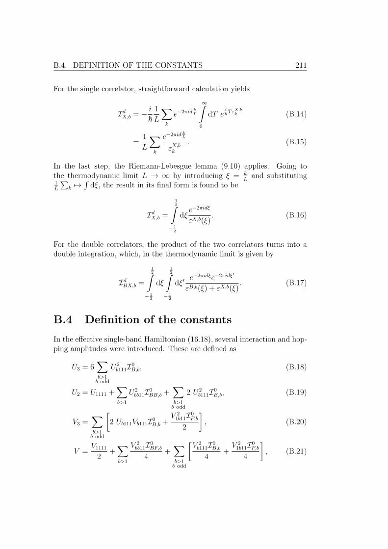
B.4. DEFINITION OF THE CONSTANTS 211
For the single correlator, straightforward calculation yields
IdX,b = − i~
1
L
∑k
e−2πid kL
∞∫0
dT ei~Tε
X,bk (B.14)
=1
L
∑k
e−2πid kL
εX,bk
. (B.15)
In the last step, the Riemann-Lebesgue lemma (9.10) applies. Going tothe thermodynamic limit L → ∞ by introducing ξ = k
Land substituting
1L
∑k 7→
∫dξ, the result in its final form is found to be
IdX,b =
12∫
− 12
dξe−2πidξ
εX,b(ξ). (B.16)
For the double correlators, the product of the two correlators turns into adouble integration, which, in the thermodynamic limit is given by
IdBX,b =
12∫
− 12
dξ
12∫
− 12
dξ′e−2πidξe−2πidξ′
εB,b(ξ) + εX,b(ξ). (B.17)
B.4 Definition of the constants
In the effective single-band Hamiltonian (16.18), several interaction and hop-ping amplitudes were introduced. These are defined as
U3 = 6∑b>1b odd
U2b111I0
B,b, (B.18)
U2 = U1111 +∑b>1
U2bb11I0
BB,b +∑b>1b odd
2 U2b111I0
B,b, (B.19)
V3 =∑b>1b odd
[2 Ub111Vb111I0
B,b +V 2
1b11I0F,b
2
], (B.20)
V =V1111
2+∑b>1
V 2bb11I0
BF,b
4+∑b>1b odd
[V 2b111I0
B,b
4+V 2
1b11I0F,b
4
], (B.21)
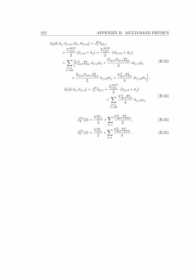
212 APPENDIX B. MULTI-BAND PHYSICS
JB[d; nj, nj+d, mj, mj+d] = JB1 δ|d|,1
+U3d,B
1111
2(nj+d + nj) +
V 3d,B1111
2(mj+d + mj)
+∑b>1b odd
[U2b111IdB,b nj+dnj +
Ub111Vb111IdB,b2
mj+dnj
+Vb111Ub111IdB,b
2nj+dmj +
V 2b111IdB,b
4mj+dmj
],
(B.22)
JF [d; nj, nj+d] = JF1 δ|d|,1 +V 3d,F
1111
2(nj+d + nj)
+∑b>1b odd
V 21b11IdF,b
4nj+dnj,
(B.23)
J(2)B (d) =
U2d1111
2+∑b>1
U2bb11IdBB,b
2, (B.24)
J(2)F (d) =
V 2d1111
2+∑b>1
V 2bb11IdBF,b
4. (B.25)
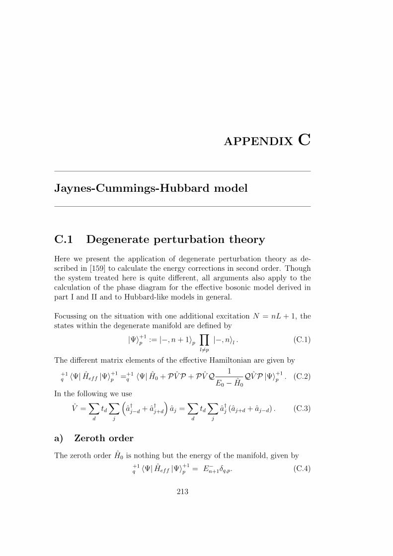
APPENDIX C
Jaynes-Cummings-Hubbard model
C.1 Degenerate perturbation theory
Here we present the application of degenerate perturbation theory as de-scribed in [159] to calculate the energy corrections in second order. Thoughthe system treated here is quite different, all arguments also apply to thecalculation of the phase diagram for the effective bosonic model derived inpart I and II and to Hubbard-like models in general.
Focussing on the situation with one additional excitation N = nL + 1, thestates within the degenerate manifold are defined by
|Ψ〉+1p := |−, n+ 1〉p
∏l 6=p
|−, n〉l . (C.1)
The different matrix elements of the effective Hamiltonian are given by
+1q 〈Ψ| Heff |Ψ〉+1
p =+1q 〈Ψ| H0 + PV P + PVQ 1
E0 − H0
QV P |Ψ〉+1p . (C.2)
In the following we use
V =∑d
td∑j
(a†j−d + a†j+d
)aj =
∑d
td∑j
a†j (aj+d + aj−d) . (C.3)
a) Zeroth order
The zeroth order H0 is nothing but the energy of the manifold, given by+1q 〈Ψ| Heff |Ψ〉+1
p = E−n+1δq,p. (C.4)
213
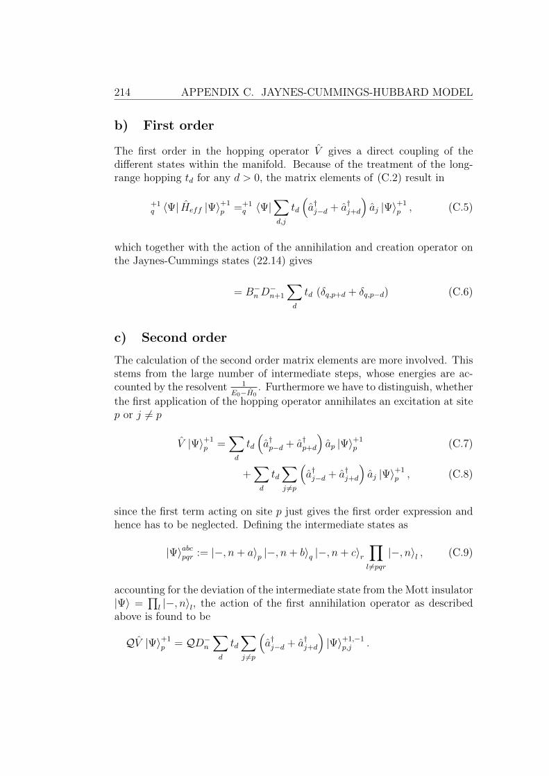
214 APPENDIX C. JAYNES-CUMMINGS-HUBBARD MODEL
b) First order
The first order in the hopping operator V gives a direct coupling of thedifferent states within the manifold. Because of the treatment of the long-range hopping td for any d > 0, the matrix elements of (C.2) result in
+1q 〈Ψ| Heff |Ψ〉+1
p =+1q 〈Ψ|
∑d,j
td
(a†j−d + a†j+d
)aj |Ψ〉+1
p , (C.5)
which together with the action of the annihilation and creation operator onthe Jaynes-Cummings states (22.14) gives
= B−nD−n+1
∑d
td (δq,p+d + δq,p−d) (C.6)
c) Second order
The calculation of the second order matrix elements are more involved. Thisstems from the large number of intermediate steps, whose energies are ac-counted by the resolvent 1
E0−H0. Furthermore we have to distinguish, whether
the first application of the hopping operator annihilates an excitation at sitep or j 6= p
V |Ψ〉+1p =
∑d
td
(a†p−d + a†p+d
)ap |Ψ〉+1
p (C.7)
+∑d
td∑j 6=p
(a†j−d + a†j+d
)aj |Ψ〉+1
p , (C.8)
since the first term acting on site p just gives the first order expression andhence has to be neglected. Defining the intermediate states as
|Ψ〉abcpqr := |−, n+ a〉p |−, n+ b〉q |−, n+ c〉r∏l 6=pqr
|−, n〉l , (C.9)
accounting for the deviation of the intermediate state from the Mott insulator|Ψ〉 =
∏l |−, n〉l, the action of the first annihilation operator as described
above is found to be
QV |Ψ〉+1p = QD−n
∑d
td∑j 6=p
(a†j−d + a†j+d
)|Ψ〉+1,−1
p,j .

C.1. DEGENERATE PERTURBATION THEORY 215
Here, a distinction whether the creation operators create on site p or anyother site is necessary, because the subsequent energy denominator givesdifferent factors in both cases. This gives
QV |Ψ〉+1p = QD−n
∑d
td
∑j 6=pj−d6=p
a†j−d |Ψ〉+1,−1p,j +
∑j 6=pj+d 6=p
a†j+d |Ψ〉+1,−1p,j
+QD−n
∑d
td
(a†p |Ψ〉
+1,−1p,p+d + a†p |Ψ〉
+1,−1p,p−d
)
= B−nD−n
∑d
td
∑j 6=pj 6=p+d
|Ψ〉+1,−1,+1p,j,j−d +
∑j 6=pj 6=p−d
|Ψ〉+1,−1,+1p,j,j+d
(C.10)
+B−n+1D−n
∑d
td
(|Ψ〉+2,−1
p,p+d + |Ψ〉+2,−1p,p−d
).
The projector Q is dropped because the intermediate states are not from thetreated manifold. For these states, the energy denominators are
1
E0 − H0
|Ψ〉+1,−1,+1p,j,j±d =
1
2E−n − E−n−1 − E−n+1
:=1
∆1
, (C.11)
1
E0 − H0
|Ψ〉+2,−1p,p±d =
1
E−n+1 + E−n − E−n+2 − E−n−1
:=1
∆+2
. (C.12)
Applying the remaining second hopping operator to the second term in (C.10)and restricting to only those output states within the manifold1 gives
PV [2nd] =B−n+1D
−n
∆+2
∑d,d′
tdtd′(a†p−d′ ap + a†p+d′ ap
)(|Ψ〉+2,−1
p,p+d + |Ψ〉+2,−1p,p−d
)=B−n+1D
−nD
−n+2
∆+2
∑d,d′
tdtd′(a†p−d′ + a†p+d′
)(|Ψ〉+1,−1
p,p+d + |Ψ〉+1,−1p,p−d
)= 2
B−n+1D−nD
−n+2B
−n−1
∆+2
∑d
t2d |Ψ〉+1p . (C.13)
In the last line, half of the terms drop out since d, d′ > 0 and because of thefinal P , the final state has to be within the degenerate manifold.
1Thus passing the final projector P.

216 APPENDIX C. JAYNES-CUMMINGS-HUBBARD MODEL
For the first term in (C.10), a simplification arises from the observation thatdue to the final P , the creation operator has to be situated at site j, whichgives
PV [1st] =B−nD
−nB−n−1
∆1
∑d′
td′∑d
td (aj+d′ + aj−d′)∑j 6=pj−d6=p
|Ψ〉+1,+1p,j−d (C.14)
+B−nD
−nB−n−1
∆1
∑d′
td′∑d
td (aj+d′ + aj−d′)∑j 6=pj+d 6=p
|Ψ〉+1,+1p,j+d .
The annihilation operator in each case has two possibilities, either beingapplied to the site p or the site j ± d. All other possibilities are ruled outbecause of the final projection P , which together with d > 0 gives:
PV [1st] = 2(L− 3)B−nD
−nB−n−1D
−n+1
∆1
∑d
t2d |Ψ〉+1p (C.15)
+B−nD
−nB−n−1D
−n+1
∆1∑dd′
td′td
[|Ψ〉+1
p−d′−d + |Ψ〉+1p+d′−d + |Ψ〉+1
p−d′+d + |Ψ〉+1p+d′+d
]Altogether, the matrix elements of the effective Hamiltonian in second orderare given by
+1q 〈Ψ| Heff |Ψ〉+1
p = δq,p E−n+1 +B−nD
−n+1
∑d
td (δq,p+d + δq,p−d) (C.16)
+ 2
(B−n+1D
−nD
−n+2B
−n−1
∆+2
+ (L− 3)B−nD
−nB−n−1D
−n+1
∆1
)∑d
t2d δq,p
+B−nD
−nB−n−1D
−n+1
∆1
∑dd′
td′td (δp−d′−d + δp+d′−d + δp−d′+d + δp+d′+d) .
For the sum in the last line, a resummation turns out to be more convenient.After some algebra, it can be rewritten as∑
dd′
td′td (δp−d′−d + δp+d′−d + δp−d′+d + δp+d′+d) (C.17)
= 2∑d
t2d δq,p +∞∑d=1
Td (δq,p−d + δq,p+d) ,

C.1. DEGENERATE PERTURBATION THEORY 217
where the modified hoppings Td are defined as
TD =D−1∑d=1
tdtD−d +∞∑
d=D+1
tdtd−D +∞∑d=1
tdtD+d. (C.18)
This finally gives the second order effective Hamiltonian for the state withan additional excitation which in this form is given by
+1q 〈Ψ| Heff |Ψ〉+1
p = δq,p E−n+1 +B−nD
−n+1
∑d
td (δq,p+d + δq,p−d) (C.19)
+ 2
(B−n+1D
−nD
−n+2B
−n−1
∆+2
+ (L− 2)B−nD
−nB−n−1D
−n+1
∆1
)∑d
t2d δq,p
+B−nD
−nB−n−1D
−n+1
∆1
∑d
Td (δp−d + δp+d) .
Applying the same method to the situation with one excitation less as wellas the (non-degenerate) Mott insulator2, the matrix elements of the effectiveHamiltonian for these cases are given by
−1q 〈Ψ| Heff |Ψ〉−1
p = δq,p E−n−1 +B−n−1D
−n
∑d
td (δq,p+d + δq,p−d) (C.20)
+ 2
(B−nD
−n−1D
−n+1B
−n−2
∆−2+ (L− 2)
B−nD−nB−n−1D
−n+1
∆1
)∑d
t2d δq,p
+B−nD
−nB−n−1D
−n+1
∆1
∑d
Td (δp−d + δp+d) .
and
〈Ψ| Heff |Ψ〉 = δq,p E−n + 2L
B−nD−nB−n−1D
−n+1
∆1
∑d
t2d δq,p (C.21)
with ∆±2 = E−n±1 + E−n − E−n±2 − E−n∓1.
2Which is naturally not necessary since simple perturbation theory suffices.


List of figures
1.1 Phase diagram of the Bose-Hubbard model . . . . . . . . . . . 151.2 Phase diagram of the disordered Bose-Hubbard model . . . . . 161.3 Phase diagram of the extended Bose-Hubbard model . . . . . 181.4 First two Wannier functions . . . . . . . . . . . . . . . . . . . 201.5 Band structure of the optical lattice . . . . . . . . . . . . . . . 211.6 Hopping as function of ηB . . . . . . . . . . . . . . . . . . . . 22
3.1 Zero hopping incompressible phases . . . . . . . . . . . . . . . 313.2 Perturbative ground state for various fermion distributions . . 333.3 Effective coupling constants . . . . . . . . . . . . . . . . . . . 353.4 Strong-coupling phase diagram . . . . . . . . . . . . . . . . . 383.5 Phase diagram for different fermion distributions . . . . . . . . 403.6 Cell-strong-coupling phase diagram . . . . . . . . . . . . . . . 413.7 Phase diagram for annealed fermions . . . . . . . . . . . . . . 423.8 Phase diagram for JF = JB . . . . . . . . . . . . . . . . . . . 433.9 Finite size scaling of the critical hopping . . . . . . . . . . . . 44
4.1 Density cut for annealed fermions . . . . . . . . . . . . . . . . 464.2 Correlations for annealed fermions . . . . . . . . . . . . . . . . 484.3 Correlations for quenched fermions . . . . . . . . . . . . . . . 494.4 Density cut for JF = JB . . . . . . . . . . . . . . . . . . . . . 504.5 Correlations for JF = JB . . . . . . . . . . . . . . . . . . . . . 51
7.1 Friedel oscillations within the Mott insulator . . . . . . . . . . 607.2 Zero-hopping phase diagram for open boundaries . . . . . . . 617.3 Phase diagram and densities for double half filling . . . . . . . 63
8.1 Feynman graph of the induced density-density interaction . . . 68
9.1 Density-density cumulant for free fermions . . . . . . . . . . . 719.2 %F -dependence of the coupling for free fermions . . . . . . . . 73
219
220 LIST OF FIGURES
9.3 Distance-dependence of the couplings for free fermions . . . . 74
9.4 Scaling behavior of the couplings for free fermions . . . . . . . 75
9.5 CDW amplitude of bosons and fermions from DMRG . . . . . 76
9.6 Direct summation of the couplings for k = 0 . . . . . . . . . . 78
9.7 Fourier transform of the couplings for free fermions . . . . . . 79
10.1 Local density from the renormalized fermion model . . . . . . 88
10.2 Fermionic versus Bosonic amplitude . . . . . . . . . . . . . . . 89
10.3 First-order correlations from the renormalized fermion model . 90
10.4 Comparison of the free fermion and the renormalized couplings 92
10.5 Fourier transformed couplings . . . . . . . . . . . . . . . . . . 93
11.1 Self-consistent determination: coherent state . . . . . . . . . . 99
11.2 Self-consistent determination: matrix product state . . . . . . 101
12.1 Zero hopping phase diagram . . . . . . . . . . . . . . . . . . . 108
12.2 Visualization of intermediate processes . . . . . . . . . . . . . 112
12.3 Analytic results for the phase diagram . . . . . . . . . . . . . 113
12.4 Boundary effects to the phase diagram . . . . . . . . . . . . . 115
12.5 Density within the different phases . . . . . . . . . . . . . . . 116
12.6 Density cut along the µB-axis . . . . . . . . . . . . . . . . . . 117
12.7 Order parameter of the phase separation . . . . . . . . . . . . 118
15.1 Generalized higher-band hopping processes . . . . . . . . . . . 128
15.2 Band coupling for any higher band . . . . . . . . . . . . . . . 130
15.3 Band coupling for odd higher bands . . . . . . . . . . . . . . . 131
17.1 Determination of the transition: plain BHM (1D) . . . . . . . 149
18.1 Experimental results transition shift . . . . . . . . . . . . . . . 152
18.2 Determination of the transition: one dimension . . . . . . . . 154
18.3 Shift of the transition in one dimension . . . . . . . . . . . . . 155
18.4 Correction of the Mott lobes in one dimension . . . . . . . . . 156
18.5 Determination of the transition: three dimensions . . . . . . . 158
18.6 Shift of the transition in three dimensions . . . . . . . . . . . 159
18.7 Correction of the Mott lobes in three dimensions . . . . . . . . 159
21.1 Discussion of the ground state of the JCHM . . . . . . . . . . 168
21.2 Mott lobes of the JCHM for zero hopping . . . . . . . . . . . 170
21.3 Comparison of the finite to infinite system phonon energy . . . 172
23.1 Phase diagram of the plain JCHM . . . . . . . . . . . . . . . . 183

LIST OF FIGURES 221
24.1 Dispersion within the fermion approximation . . . . . . . . . . 18624.2 Mott lobes for ion-chain setup . . . . . . . . . . . . . . . . . . 18724.3 Phase diagram ion chain within fermion approximation . . . . 18824.4 Critical hopping within the ion-chain setup . . . . . . . . . . . 189
A.1 Visualization of the Dirac comb potential . . . . . . . . . . . . 201

Bibliography
[1] S. Chu, Nobel Lecture: The manipulation of neutral particles, Rev.Mod. Phys. 70, 685, (1998).
[2] C. N. Cohen-Tannoudji, Nobel Lecture: Manipulating atoms with pho-tons, Rev. Mod. Phys. 70, 707, (1998).
[3] W. D. Phillips, Nobel Lecture: Laser cooling and trapping of neutralatoms, Rev. Mod. Phys. 70, 721, (1998).
[4] S. Bose, Planck’s law and light quantum hypothesis, Z. Phys. 26, 178,(1924).
[5] A. Einstein, Quantum theory of the ideal gas, Sitzungsber. Preuss.Akad. Wiss. 18, (1925).
[6] K. B. Davis, M. O. Mewes, M. R. Andrews, N. J. van Druten, D. S.Durfee, D. M. Kurn, and W. Ketterle, Bose-Einstein condensation ina gas of sodium atoms, Phys. Rev. Lett. 75, 3969, (1995).
[7] W. Ketterle, Nobel lecture: When atoms behave as waves: Bose-Einstein condensation and the atom laser, Rev. Mod. Phys. 74, 1131,(2002).
[8] M. H. Anderson, J. R. Ensher, M. R. Matthews, C. E. Wieman, andE. A. Cornell, Observation of Bose-Einstein condensation in a diluteatomic vapor, Science 269, 198, (1995).
[9] E. A. Cornell and C. E. Wieman, Nobel Lecture: Bose-Einstein conden-sation in a dilute gas, the first 70 years and some recent experiments,Rev. Mod. Phys. 74, 875, (2002).
[10] C. C. Bradley, C. A. Sackett, J. J. Tollett, and R. G. Hulet, Evidenceof Bose-Einstein condensation in an atomic gas with attractive inter-actions, Phys. Rev. Lett. 75, 1687, (1995).
223
224 BIBLIOGRAPHY
[11] B. DeMarco and D. Jin, Onset of Fermi degeneracy in a trapped atomicgas, Science 285, 1703, (1999).
[12] S. Giorgini, L. P. Pitaevskii, and S. Stringari, Theory of ultracoldatomic Fermi gases, Rev. Mod. Phys. 80, 1215, (2008).
[13] I. Bloch, J. Dalibard, and W. Zwerger, Many-body physics with ultracoldgases, Rev. Mod. Phys. 80, 885, (2008).
[14] M. P. A. Fisher, P. B. Weichman, G. Grinstein, and D. S. Fisher,Boson localization and the superfluid-insulator transition, Phys. Rev.B 40, 546, (1989).
[15] M. Greiner, O. Mandel, T. Esslinger, T. W. Hansch, and I. Bloch,Quantum phase transition from a superfluid to a Mott insulator in agas of ultracold atoms, Nature 415, 39, (2002).
[16] R. Jordens, N. Strohmaier, K. Gunter, H. Moritz, and T. Esslinger,A Mott insulator of fermionic atoms in an optical lattice, Nature 455,204, (2008).
[17] U. Schneider, L. Hackermuller, S. Will, T. Best, I. Bloch, T. A. Costi,R. W. Helmes, D. Rasch, and A. Rosch, Metallic and insulating phasesof repulsively interacting fermions in a three-dimensional optical lattice,Science 322, 1520, (2008).
[18] S. O. Demokritov, V. E. Demidov, O. Dzyapko, G. A. Melkov, A. A.Serga, B. Hillebrands, and A. N. Slavin, Bose-Einstein condensation ofquasi-equilibrium magnons at room temperature under pumping, Nature443, 430, (2006).
[19] J. Kasprzak, M. Richard, S. Kundermann, A. Baas, P. Jeambrun,J. M. J. Keeling, F. M. Marchetti, M. H. Szymanska, R. Andre, J. L.Staehli, V. Savona, P. B. Littlewood, B. Deveaud, and L. S. Dang,Bose-Einstein condensation of exciton polaritons, Nature 443, 409,(2006).
[20] F. London, The λ-phenomenon of liquid helium and the Bose-Einsteindegeneracy, Nature 141, 643, (1938).
[21] F. London, On the Bose-Einstein condensation, Phys. Rev. 54, 947,(1938).
[22] L. N. Cooper, Bound electron pairs in a degenerate Fermi gas, Phys.Rev. 104, 1189, (1956).

BIBLIOGRAPHY 225
[23] J. Bardeen, L. N. Cooper, and J. R. Schrieffer, Microscopic theory ofsuperconductivity, Phys. Rev. 106, 162, (1957).
[24] J. Bardeen, L. N. Cooper, and J. R. Schrieffer, Theory of superconduc-tivity, Phys. Rev. 108, 1175, (1957).
[25] A. J. Leggett, Bose-Einstein condensation in the alkali gases: Somefundamental concepts, Rev. Mod. Phys. 73, 307, (2001).
[26] S. Kraft, F. Vogt, O. Appel, F. Riehle, and U. Sterr, Bose-Einstein con-densation of alkaline earth atoms: 40Ca, Phys. Rev. Lett. 103, 130401,(2009).
[27] S. Stellmer, M. K. Tey, B. Huang, R. Grimm, and F. Schreck, Bose-Einstein condensation of Strontium, Phys. Rev. Lett. 103, 200401,(2009).
[28] Y. Takasu, K. Maki, K. Komori, T. Takano, K. Honda, M. Kumakura,T. Yabuzaki, and Y. Takahashi, Spin-singlet Bose-Einstein condensa-tion of two-electron atoms, Phys. Rev. Lett. 91, 040404, (2003).
[29] F. Pereira Dos Santos, J. Leonard, J. Wang, C. J. Barrelet, F. Perales,E. Rasel, C. S. Unnikrishnan, M. Leduc, and C. Cohen-Tannoudji,Bose-Einstein condensation of metastable Helium, Phys. Rev. Lett. 86,3459, (2001).
[30] A. Robert, O. Sirjean, A. Browaeys, J. Poupard, S. Nowak, D. Bo-iron, C. I. Westbrook, and A. Aspect, A Bose-Einstein condensate ofmetastable atoms, Science 292, 461, (2001).
[31] D. G. Fried, T. C. Killian, L. Willmann, D. Landhuis, S. C. Moss,D. Kleppner, and T. J. Greytak, Bose-Einstein condensation of atomicHydrogen, Phys. Rev. Lett. 81, 3811, (1998).
[32] A. Griesmaier, J. Werner, S. Hensler, J. Stuhler, and T. Pfau, Bose-Einstein condensation of Chromium, Phys. Rev. Lett. 94, 160401,(2005).
[33] A. G. Truscott, K. E. Strecker, W. I. McAlexander, G. B. Partridge,and R. G. Hulet, Observation of Fermi pressure in a gas of trappedatoms, Science 291, 2570, (2001).
[34] F. Schreck, L. Khaykovich, K. L. Corwin, G. Ferrari, T. Bourdel,J. Cubizolles, and C. Salomon, Quasipure Bose-Einstein condensateimmersed in a Fermi sea, Phys. Rev. Lett. 87, 080403, (2001).

226 BIBLIOGRAPHY
[35] Z. Hadzibabic, C. A. Stan, K. Dieckmann, S. Gupta, M. W. Zwierlein,A. Gorlitz, and W. Ketterle, Two-species mixture of quantum degener-ate Bose and Fermi gases, Phys. Rev. Lett. 88, 160401, (2002).
[36] G. Roati, F. Riboli, G. Modugno, and M. Inguscio, Fermi-Bose quan-tum degenerate 40K-87Rb mixture with attractive interaction, Phys. Rev.Lett. 89, 150403, (2002).
[37] K. Gunter, T. Stoferle, H. Moritz, M. Kohl, and T. Esslinger, Bose-Fermi mixtures in a three-dimensional optical lattice, Phys. Rev. Lett.96, 180402, (2006).
[38] S. Ospelkaus, C. Ospelkaus, O. Wille, M. Succo, P. Ernst, K. Sengstock,and K. Bongs, Localization of bosonic atoms by fermionic impurities ina three-dimensional optical lattice, Phys. Rev. Lett. 96, 180403, (2006).
[39] A. Albus, F. Illuminati, and J. Eisert, Mixtures of bosonic andfermionic atoms in optical lattices, Phys. Rev. A 68, 023606, (2003).
[40] N. Gemelke, X. Zhang, C.-L. Hung, and C. Chin, In situ observationof incompressible Mott-insulating domains in ultracold atomic gases,Nature 460, 995, (2009).
[41] W. S. Bakr, J. I. Gillen, A. Peng, S. Folling, and M. Greiner, A quantumgas microscope for detecting single atoms in a Hubbard-regime opticallattice, Nature 462, 74, (2009).
[42] T. Gericke, P. Wurtz, D. Reitz, T. Langen, and H. Ott, High-resolutionscanning electron microscopy of an ultracold quantum gas, Nat. Phys.4, 949, (2008).
[43] S. Folling, F. Gerbier, A. Widera, O. Mandel, T. Gericke, and I. Bloch,Spatial quantum noise interferometry in expanding ultracold atomclouds, Nature 434, 481, (2005).
[44] G. K. Campbell, J. Mun, M. Boyd, P. Medley, A. E. Leanhardt, L. G.Marcassa, D. E. Pritchard, and W. Ketterle, Imaging the Mott insulatorshells by using atomic clock shifts, Science 313, 649, (2006).
[45] F. Dalfovo, S. Giorgini, L. P. Pitaevskii, and S. Stringari, Theory ofBose-Einstein condensation in trapped gases, Rev. Mod. Phys. 71, 463,(1999).
BIBLIOGRAPHY 227
[46] T. Stoferle, H. Moritz, C. Schori, M. Kohl, and T. Esslinger, Transi-tion from a strongly interacting one-dimensional superfluid to a Mottinsulator, Phys. Rev. Lett. 92, 130403, (2004).
[47] C. Chin, M. Bartenstein, A. Altmeyer, S. Riedl, S. Jochim, J. H. Den-schlag, and R. Grimm, Observation of the pairing gap in a stronglyinteracting Fermi gas, Science 305, 1128, (2004).
[48] J. Stenger, S. Inouye, A. P. Chikkatur, D. M. Stamper-Kurn, D. E.Pritchard, and W. Ketterle, Bragg spectroscopy of a Bose-Einstein con-densate, Phys. Rev. Lett. 82, 4569, (1999).
[49] D. Clement, N. Fabbri, L. Fallani, C. Fort, and M. Inguscio, Multi-band spectroscopy of inhomogeneous Mott-insulator states of ultracoldbosons, New J. Phys. 11, 103030, (2009).
[50] P. T. Ernst, S. Gotze, J. S. Krauser, K. Pyka, D.-S. Luhmann,D. Pfannkuche, and K. Sengstock, Probing superfluids in optical latticesby momentum-resolved Bragg spectroscopy, Nat. Phys. 6, 56, (2010).
[51] H. Moritz, Quantum gases: Atomic superfluids see the light, Nat. Phys.6, 10, (2010).
[52] R. Folman, P. Krueger, J. Schmiedmayer, J. Denschlag, and C. Henkel,Microscopic atom optics: from wires to an atom chip, in Advances inAtomic, Molecular and Optical Physics (B. Bederson and H. Walther,eds.), vol. 48, 263, Academic Press, (2002).
[53] S. Knoop, F. Ferlaino, M. Berninger, M. Mark, H.-C. Nagerl,R. Grimm, J. P. D’Incao, and B. D. Esry, Magnetically controlled ex-change process in an ultracold atom-dimer mixture, Phys. Rev. Lett.104, 053201, (2010).
[54] R. V. Krems, Ultracold controlled chemistry, Physics 3, 10, (2010).
[55] S. Ospelkaus, K.-K. Ni, D. Wang, M. H. G. de Miranda, B. Neyen-huis, G. Quemener, P. S. Julienne, J. L. Bohn, D. S. Jin, and J. Ye,Quantum-state controlled chemical reactions of ultracold Potassium-Rubidium molecules, Science 327, 853, (2010).
[56] V. N. Efimov, Weakly-bound states of three resonantly-interacting par-ticles, Sov. Nucl. Phys. 12, 589, (1971).
228 BIBLIOGRAPHY
[57] T. Kraemer, M. Mark, P. Waldburger, J. G. Danzl, C. Chin, B. Engeser,A. D. Lange, K. Pilch, A. Jaakkola, H.-C. Nagerl, and R. Grimm,Evidence for Efimov quantum states in an ultracold gas of Caesiumatoms, Nature 440, 315, (2006).
[58] C. H. Greene, Universal insights from few-body land, Physics Today 3,40, (2010).
[59] D. Jaksch, C. Bruder, J. I. Cirac, C. W. Gardiner, and P. Zoller, Coldbosonic atoms in optical lattices, Phys. Rev. Lett. 81, 3108, (1998).
[60] L.-M. Duan, E. Demler, and M. D. Lukin, Controlling spin exchangeinteractions of ultracold atoms in optical lattices, Phys. Rev. Lett. 91,090402, (2003).
[61] A. Kuklov and B. Svistunov, Counterflow superfluidity of two-speciesultracold atoms in a commensurate optical lattice, Phys. Rev. Lett. 90,100401, (2003).
[62] T. Barthel, C. Kasztelan, I. P. McCulloch, and U. Schollwock, Mag-netism, coherent many-particle dynamics, and relaxation with ultracoldbosons in optical superlattices, Phys. Rev. A 79, 053627, (2009).
[63] T. Kinoshita, T. Wenger, and D. S. Weiss, Observation of a one-dimensional Tonks-Girardeau gas, Science 305, 1125, (2004).
[64] B. Paredes, A. Widera, V. Murg, O. Mandel, S. Folling, I. Cirac, G. V.Shlyapnikov, T. W. Hansch, and I. Bloch, Tonks-Girardeau gas of ul-tracold atoms in an optical lattice, Nature 429, 277, (2004).
[65] P. Jessen and I. H. Deutsch, Optical lattices, in Advances in Atomic,Molecular and Optical Physics (B. Bederson and H. Walther, eds.),vol. 37, 95, Academic Press, (1996).
[66] G. Grynberg and C. Robilliard, Cold atoms in dissipative optical lat-tices, Phys. Rep. 355, 335, (2001).
[67] F. Schmitt, M. Hild, and R. Roth, Phase diagram of bosons in two-colorsuperlattices from experimental parameters, Phys. Rev. A 80, 023621,(2009).
[68] B. Damski, J. Zakrzewski, L. Santos, P. Zoller, and M. Lewenstein,Atomic Bose and Anderson glasses in optical lattices, Phys. Rev. Lett.91, 080403, (2003).

BIBLIOGRAPHY 229
[69] J. E. Lye, L. Fallani, M. Modugno, D. S. Wiersma, C. Fort, and M. In-guscio, Bose-Einstein condensate in a random potential, Phys. Rev.Lett. 95, 070401, (2005).
[70] D. Clement, A. F. Varon, M. Hugbart, J. A. Retter, P. Bouyer,L. Sanchez-Palencia, D. M. Gangardt, G. V. Shlyapnikov, and A. As-pect, Suppression of transport of an interacting elongated Bose-Einstein condensate in a random potential, Phys. Rev. Lett. 95,170409, (2005).
[71] L. Fallani, J. E. Lye, V. Guarrera, C. Fort, and M. Inguscio, Ultracoldatoms in a disordered crystal of light: Towards a Bose glass, Phys. Rev.Lett. 98, 130404, (2007).
[72] R. P. Feynman, Simulating physics with computer, Int. J. Theor. Phys.21, 467, (1982).
[73] G. K. Brennen, C. M. Caves, P. S. Jessen, and I. H. Deutsch, Quantumlogic gates in optical lattices, Phys. Rev. Lett. 82, 1060, (1999).
[74] P. Treutlein, T. Steinmetz, Y. Colombe, B. Lev, P. Hommelhoff, J. Re-ichel, M. Greiner, O. Mandel, A. Widera, T. Rom, I. Bloch, and T. W.Hansch, Quantum information processing in optical lattices and mag-netic microtraps, Fortschr. Phys. 54, 702, (2006).
[75] D. N. Basov and T. Timusk, Electrodynamics of high- TC superconduc-tors, Rev. Mod. Phys. 77, 721, (2005).
[76] P. A. Lee, N. Nagaosa, and X.-G. Wen, Doping a Mott insulator:Physics of high-temperature superconductivity, Rev. Mod. Phys. 78,17, (2006).
[77] A. J. Leggett, What DO we know about high TC?, Nat. Phys. 2, 134,(2006).
[78] M. W. Zwierlein, A. Schirotzek, C. H. Schunck, and W. Ketterle,Fermionic superfluidity with imbalanced spin populations, Science 311,492, (2006).
[79] G. B. Partridge, W. Li, R. I. Kamar, Y.-a. Liao, and R. G. Hulet,Pairing and phase separation in a polarized Fermi gas, Science 311,503, (2006).
[80] M. Takamoto, F.-L. Hong, R. Higashi, and H. Katori, An optical latticeclock, Nature 435, 321, (2005).

230 BIBLIOGRAPHY
[81] E. Pazy and A. Vardi, Holstein model and Peierls instability in one-dimensional boson-fermion lattice gases, Phys. Rev. A 72, 033609,(2005).
[82] L. Mathey, D.-W. Wang, W. Hofstetter, M. D. Lukin, and E. Dem-ler, Luttinger liquid of polarons in one-dimensional boson-fermion mix-tures, Phys. Rev. Lett. 93, 120404, (2004).
[83] M. Lewenstein, L. Santos, M. A. Baranov, and H. Fehrmann, AtomicBose-Fermi mixtures in an optical lattice, Phys. Rev. Lett. 92, 050401,(2004).
[84] T. Best, S. Will, U. Schneider, L. Hackermuller, D. van Oosten,I. Bloch, and D.-S. Luhmann, Role of interactions in 87Rb-40K Bose-Fermi mixtures in a three-dimensional optical lattice, Phys. Rev. Lett.102, 030408, (2009).
[85] J. Catani, L. De Sarlo, G. Barontini, F. Minardi, and M. Inguscio,Degenerate Bose-Bose mixture in a three-dimensional optical lattice,Phys. Rev. A 77, 011603, (2008).
[86] D. S. Luhmann, K. Bongs, K. Sengstock, and D. Pfannkuche, Self-trapping of bosons and fermions in optical lattices, Phys. Rev. Lett.101, 050402, (2008).
[87] R. M. Lutchyn, S. Tewari, and S. Das Sarma, Boson Hubbard modelwith weakly coupled fermions, Phys. Rev. B 78, 220504(R), (2008).
[88] L. Pollet, C. Kollath, U. Schollwock, and M. Troyer, Mixture of bosonicand spin-polarized fermionic atoms in an optical lattice, Phys. Rev. A77, 023608, (2008).
[89] L. Pollet, M. Troyer, K. Van Houcke, and S. M. A. Rombouts, Phasediagram of Bose-Fermi mixtures in one-dimensional optical lattices,Phys. Rev. Lett. 96, 190402, (2006).
[90] S. Tewari, R. M. Lutchyn, and S. D. Sarma, Effects of fermions on thesuperfluid-insulator phase diagram of the Bose-Hubbard model, Phys.Rev. B 80, 054511, (2009).
[91] R. Grimm, M. Weidemuller, and Y. B. Ovchinnikov, Optical dipoletraps for neutral atoms, in Advances in Atomic, Molecular and OpticalPhysics (B. Bederson and H. Walther, eds.), vol. 42, 95, AcademicPress, (2000).

BIBLIOGRAPHY 231
[92] J. Reppy, 4He as a dilute bose gas, Physica B+C 126, 335, (1984).
[93] S. Doniach, Quantum fluctuations in two-dimensional superconductors,Phys. Rev. B 24, 5063, (1981).
[94] M. P. A. Fisher and G. Grinstein, Quantum critical phenomena incharged superconductors, Phys. Rev. Lett. 60, 208, (1988).
[95] V. L. Berezinsky, Destruction of long range order in one-dimensionaland two-dimensional systems having a continuous symmetry group. 1.Classical systems, Sov. Phys. JETP 32, 493, (1971).
[96] J. M. Kosterlitz and D. J. Thouless, Ordering, metastability and phasetransitions in two-dimensional systems, J. Phys. C 6, 1181, (1973).
[97] J. K. Freericks and H. Monien, Strong-coupling expansions for the pureand disordered Bose-Hubbard model, Phys. Rev. B 53, 2691, (1996).
[98] H. Bethe, Zur Theorie der Metalle, Z. Phys. A 71, 205, (1931).
[99] T. Giamarchi, Quantum physics in one dimension, vol. 121, of Inter-national Series of Monographs on Physics, Oxford: Clarendon Press,(2004).
[100] F. D. M. Haldane, Effective harmonic-fluid approach to low-energyproperties of one-dimensional quantum fluids, Phys. Rev. Lett. 47,1840, (1981).
[101] E. Miranda, Introduction to bosonization, Braz. J. Phys. 33, 3, (2003).
[102] M. A. Cazalilla, Bosonizing one-dimensional cold atomic gases, J. Phys.B 37, S1, (2004).
[103] S. Eggert, One-dimensional quantum wires: A pedestrian approach tobosonization, in Theoretical Survey of One Dimensional Wire Systems(Y. K. et al., ed.), ch. 2, Seoul: Sowha Publishing, (2007).
[104] M. E. Fisher, M. N. Barber, and D. Jasnow, Helicity modulus, super-fluidity, and scaling in isotropic systems, Phys. Rev. A 8, 1111, (1973).
[105] S. Rapsch, U. Schollwock, and W. Zwerger, Density matrix-renormalization group for disordered bosons in one dimension, Euro-phys. Lett. 46, 559, (1999).
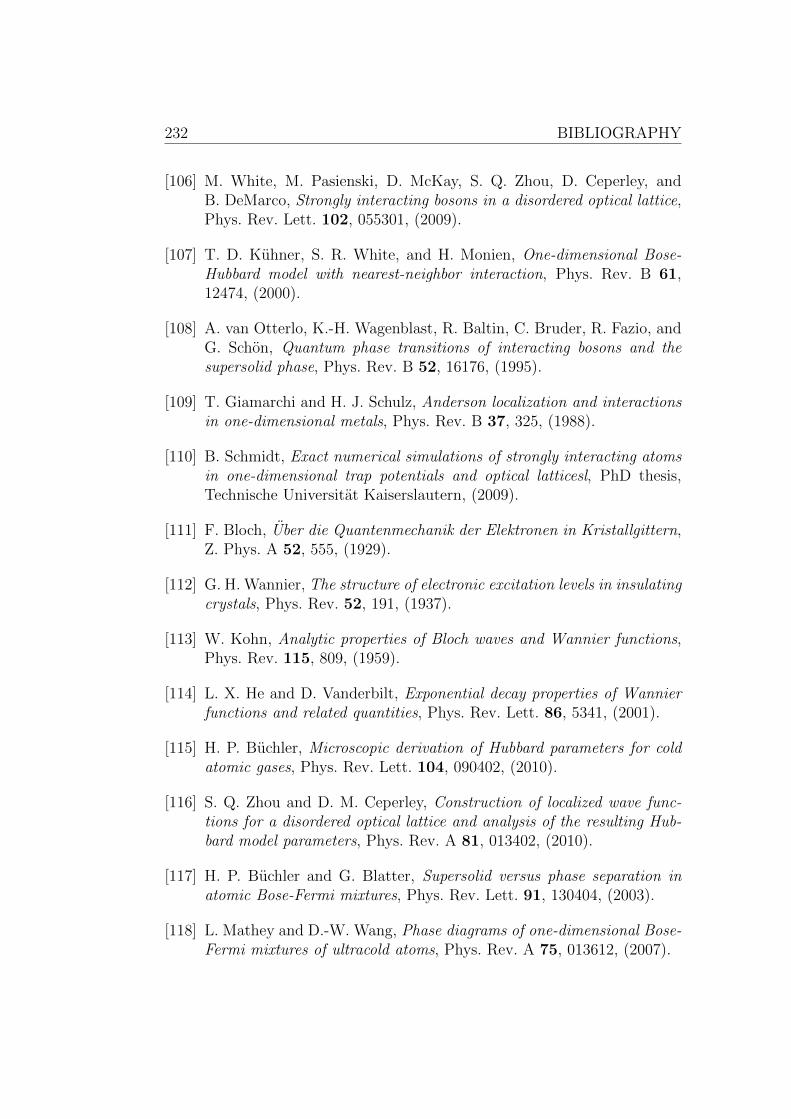
232 BIBLIOGRAPHY
[106] M. White, M. Pasienski, D. McKay, S. Q. Zhou, D. Ceperley, andB. DeMarco, Strongly interacting bosons in a disordered optical lattice,Phys. Rev. Lett. 102, 055301, (2009).
[107] T. D. Kuhner, S. R. White, and H. Monien, One-dimensional Bose-Hubbard model with nearest-neighbor interaction, Phys. Rev. B 61,12474, (2000).
[108] A. van Otterlo, K.-H. Wagenblast, R. Baltin, C. Bruder, R. Fazio, andG. Schon, Quantum phase transitions of interacting bosons and thesupersolid phase, Phys. Rev. B 52, 16176, (1995).
[109] T. Giamarchi and H. J. Schulz, Anderson localization and interactionsin one-dimensional metals, Phys. Rev. B 37, 325, (1988).
[110] B. Schmidt, Exact numerical simulations of strongly interacting atomsin one-dimensional trap potentials and optical latticesl, PhD thesis,Technische Universitat Kaiserslautern, (2009).
[111] F. Bloch, Uber die Quantenmechanik der Elektronen in Kristallgittern,Z. Phys. A 52, 555, (1929).
[112] G. H. Wannier, The structure of electronic excitation levels in insulatingcrystals, Phys. Rev. 52, 191, (1937).
[113] W. Kohn, Analytic properties of Bloch waves and Wannier functions,Phys. Rev. 115, 809, (1959).
[114] L. X. He and D. Vanderbilt, Exponential decay properties of Wannierfunctions and related quantities, Phys. Rev. Lett. 86, 5341, (2001).
[115] H. P. Buchler, Microscopic derivation of Hubbard parameters for coldatomic gases, Phys. Rev. Lett. 104, 090402, (2010).
[116] S. Q. Zhou and D. M. Ceperley, Construction of localized wave func-tions for a disordered optical lattice and analysis of the resulting Hub-bard model parameters, Phys. Rev. A 81, 013402, (2010).
[117] H. P. Buchler and G. Blatter, Supersolid versus phase separation inatomic Bose-Fermi mixtures, Phys. Rev. Lett. 91, 130404, (2003).
[118] L. Mathey and D.-W. Wang, Phase diagrams of one-dimensional Bose-Fermi mixtures of ultracold atoms, Phys. Rev. A 75, 013612, (2007).
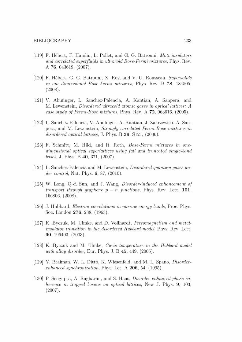
BIBLIOGRAPHY 233
[119] F. Hebert, F. Haudin, L. Pollet, and G. G. Batrouni, Mott insulatorsand correlated superfluids in ultracold Bose-Fermi mixtures, Phys. Rev.A 76, 043619, (2007).
[120] F. Hebert, G. G. Batrouni, X. Roy, and V. G. Rousseau, Supersolidsin one-dimensional Bose-Fermi mixtures, Phys. Rev. B 78, 184505,(2008).
[121] V. Ahufinger, L. Sanchez-Palencia, A. Kantian, A. Sanpera, andM. Lewenstein, Disordered ultracold atomic gases in optical lattices: Acase study of Fermi-Bose mixtures, Phys. Rev. A 72, 063616, (2005).
[122] L. Sanchez-Palencia, V. Ahufinger, A. Kantian, J. Zakrzewski, A. San-pera, and M. Lewenstein, Strongly correlated Fermi-Bose mixtures indisordered optical lattices, J. Phys. B 39, S121, (2006).
[123] F. Schmitt, M. Hild, and R. Roth, Bose-Fermi mixtures in one-dimensional optical superlattices using full and truncated single-bandbases, J. Phys. B 40, 371, (2007).
[124] L. Sanchez-Palencia and M. Lewenstein, Disordered quantum gases un-der control, Nat. Phys. 6, 87, (2010).
[125] W. Long, Q.-f. Sun, and J. Wang, Disorder-induced enhancement oftransport through graphene p − n junctions, Phys. Rev. Lett. 101,166806, (2008).
[126] J. Hubbard, Electron correlations in narrow energy bands, Proc. Phys.Soc. London 276, 238, (1963).
[127] K. Byczuk, M. Ulmke, and D. Vollhardt, Ferromagnetism and metal-insulator transition in the disordered Hubbard model, Phys. Rev. Lett.90, 196403, (2003).
[128] K. Byczuk and M. Ulmke, Curie temperature in the Hubbard modelwith alloy disorder, Eur. Phys. J. B 45, 449, (2005).
[129] Y. Braiman, W. L. Ditto, K. Wiesenfeld, and M. L. Spano, Disorder-enhanced synchronization, Phys. Let. A 206, 54, (1995).
[130] P. Sengupta, A. Raghavan, and S. Haas, Disorder-enhanced phase co-herence in trapped bosons on optical lattices, New J. Phys. 9, 103,(2007).
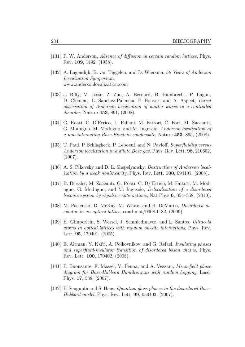
234 BIBLIOGRAPHY
[131] P. W. Anderson, Absence of diffusion in certain random lattices, Phys.Rev. 109, 1492, (1958).
[132] A. Lagendijk, B. van Tiggelen, and D. Wiersma, 50 Years of AndersonLocalization Symposium,www.andersonlocalization.com
[133] J. Billy, V. Josse, Z. Zuo, A. Bernard, B. Hambrecht, P. Lugan,D. Clement, L. Sanchez-Palencia, P. Bouyer, and A. Aspect, Directobservation of Anderson localization of matter waves in a controlleddisorder, Nature 453, 891, (2008).
[134] G. Roati, C. D’Errico, L. Fallani, M. Fattori, C. Fort, M. Zaccanti,G. Modugno, M. Modugno, and M. Inguscio, Anderson localization ofa non-interacting Bose-Einstein condensate, Nature 453, 895, (2008).
[135] T. Paul, P. Schlagheck, P. Leboeuf, and N. Pavloff, Superfluidity versusAnderson localization in a dilute Bose gas, Phys. Rev. Lett. 98, 210602,(2007).
[136] A. S. Pikovsky and D. L. Shepelyansky, Destruction of Anderson local-ization by a weak nonlinearity, Phys. Rev. Lett. 100, 094101, (2008).
[137] B. Deissler, M. Zaccanti, G. Roati, C. D/’Errico, M. Fattori, M. Mod-ugno, G. Modugno, and M. Inguscio, Delocalization of a disorderedbosonic system by repulsive interactions, Nat Phys 6, 354–358, (2010).
[138] M. Pasienski, D. McKay, M. White, and B. DeMarco, Disordered in-sulator in an optical lattice, cond-mat/0908.1182, (2009).
[139] H. Gimperlein, S. Wessel, J. Schmiedmayer, and L. Santos, Ultracoldatoms in optical lattices with random on-site interactions, Phys. Rev.Lett. 95, 170401, (2005).
[140] E. Altman, Y. Kafri, A. Polkovnikov, and G. Refael, Insulating phasesand superfluid-insulator transition of disordered boson chains, Phys.Rev. Lett. 100, 170402, (2008).
[141] P. Buonsante, F. Massel, V. Penna, and A. Vezzani, Mean-field phasediagram for Bose-Hubbard Hamiltonians with random hopping, LaserPhys. 17, 538, (2007).
[142] P. Sengupta and S. Haas, Quantum glass phases in the disordered Bose-Hubbard model, Phys. Rev. Lett. 99, 050403, (2007).

BIBLIOGRAPHY 235
[143] R. Roth and K. Burnett, Phase diagram of bosonic atoms in two-colorsuperlattices, Phys. Rev. A 68, 023604, (2003).
[144] X. L. Deng, R. Citro, A. Minguzzi, and E. Orignac, Phase diagramand momentum distribution of an interacting Bose gas in a bichromaticlattice, Phys. Rev. A 78, 013625, (2008).
[145] G. Roux, T. Barthel, I. P. McCulloch, C. Kollath, U. Schollwock, andT. Giamarchi, Quasiperiodic Bose-Hubbard model and localization inone-dimensional cold atomic gases, Phys. Rev. A 78, 023628, (2008).
[146] T. Roscilde, Bosons in one-dimensional incommensurate superlattices,Phys. Rev. A 77, 063605, (2008).
[147] U. Gavish and Y. Castin, Matter-wave localization in disordered coldatom lattices, Phys. Rev. Lett. 95, 020401, (2005).
[148] B. Horstmann, J. I. Cirac, and T. Roscilde, Dynamics of localizationphenomena for hard-core bosons in optical lattices, Phys. Rev. A 76,043625, (2007).
[149] K. V. Krutitsky, M. Thorwart, R. Egger, and R. Graham, Ultracoldbosons in lattices with binary disorder, Phys. Rev. A 77, 053609, (2008).
[150] M. Iskin and J. K. Freericks, Dynamical mean-field theory for light-fermion–heavy-boson mixtures on optical lattices, Phys. Rev. A 80,053623, (2009).
[151] L. M. Falicov and J. C. Kimball, Simple model for semiconductor-metaltransitions: SmB6 and transition-metal oxides, Phys. Rev. Lett. 22,997, (1969).
[152] D. Semmler, K. Byczuk, and W. Hofstetter, Mott-Hubbard and An-derson metal-insulator transitions in correlated lattice fermions withbinary disorder, Phys. Rev. B 81, 115111, (2010).
[153] P. Buonsante, F. Massel, V. Penna, and A. Vezzani, Mean-field descrip-tion of ultracold bosons on disordered two-dimensional optical lattices,J. Phys. B 40, F265, (2007).
[154] P. Buonsante, V. Penna, A. Vezzani, and P. B. Blakie, Mean-field phasediagram of cold lattice bosons in disordered potentials, Phys. Rev. A 76,011602, (2007).

236 BIBLIOGRAPHY
[155] U. Bissbort and W. Hofstetter, Stochastic mean-field theory for thedisordered Bose-Hubbard model, Europhys. Lett. 86, 50007, (2009).
[156] A. Zujev, A. Baldwin, R. T. Scalettar, V. G. Rousseau, P. J. H. Den-teneer, and M. Rigol, Superfluid and Mott-insulator phases of one-dimensional Bose-Fermi mixtures, Phys. Rev. A 78, 033619, (2008).
[157] P. Buonsante, V. Penna, and A. Vezzani, Fractional-filling loopholeinsulator domains for ultracold bosons in optical superlattices, Phys.Rev. A 70, 061603, (2004).
[158] H. Fehrmann, M. Baranov, M. Lewenstein, and L. Santos, Quantumphases of Bose-Fermi mixtures in optical lattices, Opt. Express 12, 55,(2004).
[159] D. J. Klein, Degenerate perturbation theory, J. Chem. Phys. 61, 786,(1974).
[160] A. Sanpera, A. Kantian, L. Sanchez-Palencia, J. Zakrzewski, andM. Lewenstein, Atomic Fermi-Bose mixtures in inhomogeneous andrandom lattices: From Fermi glass to quantum spin glass and quantumpercolation, Phys. Rev. Lett. 93, 040401, (2004).
[161] A. Mering, Bose-Fermi-Gemische in eindimensionalen Gittern, Diplo-marbeit, Technische Universitat Kaiserslautern, (2005).
[162] R. Roth and K. Burnett, Quantum phases of atomic boson-fermionmixtures in optical lattices, Phys. Rev. A 69, 021601, (2004).
[163] U. Schollwock, The density-matrix renormalization group, Rev. Mod.Phys. 77, 259, (2005).
[164] The ALPS project (Algorithms and Libraries for Physics Simulations),http://alps.comp-phys.org/mediawiki/index.php/Main Page
[165] A. Albuquerque, F. Alet, P. Corboz, P. Dayal, A. Feiguin, S. Fuchs,L. Gamper, E. Gull, S. Gurtler, A. Honecker, R. Igarashi, M. Korner,A. Kozhevnikov, A. Lauchli, S. Manmana, M. Matsumoto, I. Mc-Culloch, F. Michel, R. Noack, G. Pawlowski, L. Pollet, T. Pruschke,U. Schollwock, S. Todo, S. Trebst, M. Troyer, P. Werner, and S. Wes-sel, The ALPS project release 1.3: Open-source software for stronglycorrelated systems, J. Magn. Magn. Mater. 310, 1187, (2007).

BIBLIOGRAPHY 237
[166] R. Fazio, S. Montangero, G. D. Chiara, D. Rossini, and M. Rizzi, Par-allel open well-adapting DMRG enhanced research with power,http://www.qti.sns.it/dmrg/phome.html
[167] I. P. McCulloch, From density-matrix renormalization group to matrixproduct states, J. Stat. Mech: Theory Exp. 2007, P10014, (2007).
[168] G. Vidal, Efficient Classical Simulation of Slightly Entangled QuantumComputations, Phys. Rev. Lett. 91, 147902, (2003).
[169] G. Vidal, Classical simulation of infinite-size quantum lattice systemsin one spatial dimension, Phys. Rev. Lett. 98, 070201, (2007).
[170] N. Teichmann, D. Hinrichs, M. Holthaus, and A. Eckardt, Bose-Hubbard phase diagram with arbitrary integer filling, Phys. Rev. B 79,100503(2009), (2009).
[171] M. Ohliger and A. Pelster, Green’s function approach to the Bose-Hubbard model, (2008).
[172] B. Bradlyn, F. E. A. dos Santos, and A. Pelster, Effective action ap-proach for quantum phase transitions in bosonic lattices, Phys. Rev. A79, 013615, (2009).
[173] F. E. A. dos Santos and A. Pelster, Quantum phase diagram of bosonsin optical lattices, Phys. Rev. A 79, 013614, (2009).
[174] P. Buonsante, V. Penna, and A. Vezzani, Fractional-filling Mott do-mains in two-dimensional optical superlattices, Phys. Rev. A 72,031602, (2005).
[175] P. Buonsante, V. Penna, and A. Vezzani, Strong-coupling expansionsfor the topologically inhomogeneous Bose-Hubbard model, Phys. Rev. B70, 184520, (2004).
[176] P. Buonsante and A. Vezzani, Cell strong-coupling perturbative ap-proach to the phase diagram of ultracold bosons in optical superlattices,Phys. Rev. A 72, 013614, (2005).
[177] P. Buonsante and A. Vezzani, Phase diagram for ultracold bosons inoptical lattices and superlattices, Phys. Rev. A 70, 033608, (2004).
[178] V. G. Rousseau, D. P. Arovas, M. Rigol, F. Hebert, G. G. Batrouni,and R. T. Scalettar, Exact study of the one-dimensional boson Hubbardmodel with a superlattice potential, Phys. Rev. B 73, 174516, (2006).
238 BIBLIOGRAPHY
[179] H. Fehrmann, M. A. Baranov, B. Damski, M. Lewenstein, and L. San-tos, Mean-field theory of Bose-Fermi mixtures in optical lattices, Opt.Commun. 243, 23, (2004).
[180] M. Cramer, J. Eisert, and F. Illuminati, Inhomogeneous atomic Bose-Fermi mixtures in cubic lattices, Phys. Rev. Lett. 93, 190405, (2004).
[181] D. van Oosten, P. van der Straten, and H. T. C. Stoof, Quantum phasesin an optical lattice, Phys. Rev. A 63, 053601, (2001).
[182] A. W. Sandvik, Quantum monte carlo simulations of bosonic andfermionic impurities in a two-dimensional hard-core boson system,Phys. Rev. Lett. 101, 120405, (2008).
[183] T. D. Kuhner and H. Monien, Phases of the one-dimensional Bose-Hubbard model, Phys. Rev. B 58, 14741(R), (1998).
[184] J. M. Luttinger, An exactly soluble model of a many-fermion system,J. Math. Phys. 4, 1154, (1963).
[185] S. Tomonaga, Remarks on Bloch’s method of sound waves applied tomany-fermion problems, Progr. Theoret. Phys. 5, 544, (1950).
[186] J. Voit, One-dimensional Fermi liquids, Rep. Prog. Phys. 58, 977,(1995).
[187] F. Schwabl, Statistische Mechanik, Springer, (2000).
[188] P. N. Suding and R. M. Ziff, Site percolation thresholds for Archimedeanlattices, Phys. Rev. E 60, 275, (1999).
[189] P. Buonsante, F. Massel, V. Penna, and A. Vezzani, Gutzwiller ap-proach to the Bose-Hubbard model with random local impurities, Phys.Rev. A 79, 013623, (2009).
[190] R. V. Pai, R. Pandit, H. R. Krishnamurthy, and S. Ramasesha,One-dimensional disordered bosonic Hubbard model: A density-matrixrenormalization group study, Phys. Rev. Lett. 76, 2937, (1996).
[191] L. Pollet, N. V. Prokof’ev, B. V. Svistunov, and M. Troyer, Absenceof a direct superfluid to Mott insulator transition in disordered Bosesystems, Phys. Rev. Lett. 103, 140402, (2009).
[192] V. Gurarie, L. Pollet, N. V. Prokof’ev, B. V. Svistunov, and M. Troyer,Phase diagram of the disordered Bose-Hubbard model, Phys. Rev. B 80,214519, (2009).
BIBLIOGRAPHY 239
[193] S. F. Edwards and P. W. Anderson, Theory of spin glasses, J. Phys. F5, 965, (1975).
[194] S. Morrison, Characterization of quantum phase transitions in dissi-pative cavity QED systems and cold atoms with disorder, PhD thesis,Leopold-Franzens-Universitat Innsbruck, (2008).
[195] E. Kim and M. H. W. Chan, Probable observation of a supersolid He-lium phase, Nature 427, 225, (2004).
[196] D. J. Thouless, The flow of a dense superfluid, Ann. Phys. 52, 403,(1969).
[197] A. F. Andreev and I. M. Lifshitz, Quantum theory of defects in crystals,Sov. Phys. JETP 29, 1107, (1969).
[198] A. J. Leggett, Can a Solid Be ”Superfluid”?, Phys. Rev. Lett. 25, 1543,(1970).
[199] S. Balibar, The enigma of supersolidity, Nature 464, 176, (2010).
[200] G. G. Batrouni and R. T. Scalettar, Phase separation in supersolids,Phys. Rev. Lett. 84, 1599, (2000).
[201] P. Sengupta, L. P. Pryadko, F. Alet, M. Troyer, and G. Schmid, Super-solids versus phase separation in two-dimensional lattice bosons, Phys.Rev. Lett. 94, 207202, (2005).
[202] B. Capogrosso-Sansone, C. Trefzger, M. Lewenstein, P. Zoller, andG. Pupillo, Quantum phases of cold polar molecules in two-dimensionaloptical lattices, Phys. Rev. Lett. 104, 125301, (2010).
[203] T. Mishra, R. V. Pai, S. Ramanan, M. S. Luthra, and B. P. Das,Supersolid and solitonic phases in the one-dimensional extended Bose-Hubbard model, Phys. Rev. A 80, 043614, (2009).
[204] P. P. Orth, D. L. Bergman, and K. Le Hur, Supersolidity of cold-atom Bose-Fermi mixtures in optical lattices, Phys. Rev. A 80, 023624,(2009).
[205] I. Titvinidze, M. Snoek, and W. Hofstetter, Supersolid Bose-Fermimixtures in optical lattices, Phys. Rev. Lett. 100, 100401, (2008).
[206] A. Hubener, M. Snoek, and W. Hofstetter, Magnetic phases of two-component ultracold bosons in an optical lattice, Phys. Rev. B 80,245109, (2009).

240 BIBLIOGRAPHY
[207] T. Keilmann, J. I. Cirac, and T. Roscilde, Dynamical creation of asupersolid in asymmetric mixtures of bosons, Phys. Rev. Lett. 102,255304, (2009).
[208] S. G. Soyler, B. Capogrosso-Sansone, N. V. Prokof’ev, and B. V. Svis-tunov, Sign-alternating interaction mediated by strongly correlated lat-tice bosons, New J. Phys. 11, 073036, (2009).
[209] L. Mathey, I. Danshita, and C. W. Clark, Creating a supersolid inone-dimensional Bose mixtures, Phys. Rev. A 79, 011602, (2009).
[210] I. Titvinidze, M. Snoek, and W. Hofstetter, Generalized dynamicalmean-field theory for Bose-Fermi mixtures in optical lattices, Phys.Rev. B 79, 144506, (2009).
[211] L. Pollet, S. Rombouts, K. Heyde, and J. Dukelsky, Bosons confined inoptical lattices: The numerical renormalization group revisited, Phys.Rev. A 69, 043601, (2004).
[212] E. Altman, W. Hofstetter, E. Demler, and M. D. Lukin, Phase diagramof two-component bosons on an optical lattice, New J. Phys. 5, 113,(2003).
[213] H. P. Buchler and G. Blatter, Phase separation of atomic Bose-Fermimixtures in an optical lattice, Phys. Rev. A 69, 063603, (2004).
[214] G. Mazzarella, How the effective boson-boson interaction works inBose-Fermi mixtures in periodic geometries, Eur. Phys. J. D 50, 61,(2008).
[215] K. Yang, Superfluid-insulator transition and fermion pairing in Bose-Fermi mixtures, Phys. Rev. B 77, 085115, (2008).
[216] D. H. Santamore and E. Timmermans, Fermion-mediated interactionsin a dilute Bose-Einstein condensate, Phys. Rev. A 78, 013619, (2008).
[217] G. Refael and E. Demler, Superfluid-insulator transition in Fermi-Bosemixtures and the orthogonality catastrophe, Phys. Rev. B 77, 144511,(2008).
[218] J. Friedel, The distribution of electrons round impurities in monovalentmetals, Philos. Mag. 43, 153, (1952).
[219] G. Bedurftig, B. Brendel, H. Frahm, and R. M. Noack, Friedel oscilla-tions in the open Hubbard chain, Phys. Rev. B 58, 10225, (1998).
BIBLIOGRAPHY 241
[220] G. D. Mahan, Many-particle physics, Plenum Press, New York,third ed., (2000).
[221] S. A. Soffing, M. Bortz, I. Schneider, A. Struck, M. Fleischhauer,and S. Eggert, Wigner crystal versus Friedel oscillations in the one-dimensional Hubbard model, Phys. Rev. B 79, 195114, (2009).
[222] J. Stepisnik, Validity limits of Gaussian approximation in cumulantexpansion for diffusion attenuation of spin echo, Physica B 270, 110,(1999).
[223] C. W. Gardiner, Handbook of Stochastic Methods, Berlin: Springer,(1985).
[224] M. Fleischhauer and S. F. Yelin, Radiative atom-atom interactions inoptically dense media: Quantum corrections to the Lorentz-Lorenz for-mula, Phys. Rev. A 59, 2427, (1999).
[225] R. Kubo, Generalized cumulant expansion method, J. Phys. Soc. Jpn.17, 1100, (1962).
[226] R. Kubo, Stochastic Liouville equations, J. Math. Phys. 4, 174, (1963).
[227] W. H. Louisell, Quantum statistical properties of radiation, Wiley NewYork, (1973).
[228] H. Carmichael, An Open Systems Approach to Quantum Optics,Springer-Verlag, (1993).
[229] S. Bochner and K. Chandrasekharan, Fourier Transforms, PrincetonUniversity Press, (1949).
[230] M. A. Ruderman and C. Kittel, Indirect exchange coupling of nuclearmagnetic moments by conduction electrons, Phys. Rev. 96, 99, (1954).
[231] T. Kasuya, A theory of metallic ferromagnetism and antiferromag-netism on Zeners model, Progr. Theoret. Phys. 16, 45, (1956).
[232] K. Yosida, Magnetic properties of Cu-Mn alloys, Phys. Rev. 106, 893,(1957).
[233] L. van Hove, The occurrence of singularities in the elastic frequencydistribution of a crystal, Phys. Rev. 89, 1189, (1953).
[234] E. Lieb, T. Schultz, and D. Mattis, Two soluble models of an antifer-romagnetic chain, Ann. Phys. 16, 407, (1961).
242 BIBLIOGRAPHY
[235] G. C. Wick, The evaluation of the collision matrix, Phys. Rev. 80, 268,(1950).
[236] F. Schwabl, Quantenmechanik fur Fortgeschrittene, Berlin: Springer-Verlag, second ed., (2000).
[237] M. Abramowitz and I. A. Stegun, Handbook of mathematical functions,New York: Dover, (1964).
[238] R. J. Glauber, Coherent and incoherent states of the radiation field,Phys. Rev. 131, 2766, (1963).
[239] N. Teichmann, D. Hinrichs, M. Holthaus, and A. Eckardt, Processchain approach to the Bose-Hubbard model: Ground-state propertiesand phase diagram, Phys. Rev. B 79, 224515, (2009).
[240] A. Eckardt, Process-chain approach to high-order perturbation calculusfor quantum lattice models, Phys. Rev. B 79, 195131, (2009).
[241] P. Bak and R. Bruinsma, One-dimensional Ising model and the com-plete devil’s staircase, Phys. Rev. Lett. 49, 249, (1982).
[242] F. J. Burnell, M. M. Parish, N. R. Cooper, and S. L. Sondhi, Devil’sstaircases and supersolids in a one-dimensional dipolar Bose gas, Phys.Rev. B 80, 174519, (2009).
[243] S. Will, T. Best, U. Schneider, L. Hackermuller, D.-S. Luhmann, andI. Bloch, Time-resolved observation of coherent multi-body interactionsin quantum phase revivals, Nature 465, 197, (2010).
[244] P. R. Johnson, E. Tiesinga, J. V. Porto, and C. J. Williams, Effec-tive three-body interactions of neutral bosons in optical lattices, New J.Phys. 11, 093022, (2009).
[245] J. Larson, A. Collin, and J.-P. Martikainen, Multiband bosons in opticallattices, Phys. Rev. A 79, 033603, (2009).
[246] A. Collin, J. Larson, and J.-P. Martikainen, Quantum states of p-bandbosons in optical lattices, Phys. Rev. A 81, 023605, (2010).
[247] M. Cramer, S. Ospelkaus, C. Ospelkaus, K. Bongs, K. Sengstock, andJ. Eisert, Do mixtures of bosonic and fermionic atoms adiabaticallyheat up in optical lattices?, Phys. Rev. Lett. 100, 140409, (2008).

BIBLIOGRAPHY 243
[248] C. N. Varney, V. G. Rousseau, and R. T. Scalettar, Quantum montecarlo study of the visibility of one-dimensional Bose-Fermi mixtures,Phys. Rev. A 77, 041608, (2008).
[249] R. M. Lutchyn, S. Tewari, and S. Das Sarma, Loss of superfluidity byfermions in the boson Hubbard model on an optical lattice, Phys. Rev.A 79, 011606(R), (2009).
[250] I. Titvinidze, M. Snoek, and W. Hofstetter, Resonant superfluidity inan optical lattice, cond-mat/0912.1589, (2009).
[251] J. Bunemann, A slave-boson mean-field theory for general multi-bandHubbard models, cond-mat/1002.3228, (2010).
[252] M. Ohliger, M. Cramer, and J. Eisert, Multi-band Gutzwiller ansatz forinteracting bosons and fermions for finite temperature, Private commu-nication.
[253] A. Isacsson and S. M. Girvin, Multiflavor bosonic Hubbard models in thefirst excited Bloch band of an optical lattice, Phys. Rev. A 72, 053604,(2005).
[254] G. Mazzarella, S. M. Giampaolo, and F. Illuminati, Extended BoseHubbard model of interacting bosonic atoms in optical lattices: Fromsuperfluidity to density waves, Phys. Rev. A 73, 013625, (2006).
[255] L. Amico, G. Mazzarella, S. Pasini, and F. S. Cataliotti, Hidden orderin bosonic gases confined in one-dimensional optical lattices, New J.Phys. 12, 013002, (2010).
[256] M. E. Gehm, Properties of 6Li,http://www.phy.duke.edu/research/photon/qoptics/techdocs
[257] D. A. Steck, 85Rb D-Line Data,http://steck.us/alkalidata
[258] D. A. Steck, 87Rb D-Line Data,http://steck.us/alkalidata
[259] NIST Atomic Spectra Database,http://www.nist.gov/physlab/data/asd.cfm
[260] H. Feshbach, Unified theory of nuclear reactions, Ann. Phys. 5, 357,(1958).
244 BIBLIOGRAPHY
[261] U. Fano, Effects of configuration interaction on intensities and phaseshifts, Phys. Rev. 124, 1866, (1961).
[262] P. Risberg, A revision of the term systems for Na and K based onhollow-cathode observations, Arkiv For Fysik 10, 583, (1956).
[263] M. Olshanii, Atomic scattering in the presence of an external con-finement and a gas of impenetrable bosons, Phys. Rev. Lett. 81, 938,(1998).
[264] I. Bouchoule, M. Morinaga, C. Salomon, and D. S. Petrov, Caesiumgas strongly confined in one dimension: Sideband cooling and collisionalproperties, Phys. Rev. A 65, 033402, (2002).
[265] A. van Amerongen, One dimensional Bose gas on an atom chip, PhDthesis, University of Amsterdam, (2008).
[266] T. Volz, S. Durr, S. Ernst, A. Marte, and G. Rempe, Characterizationof elastic scattering near a Feshbach resonance in 87Rb, Phys. Rev. A68, 010702, (2003).
[267] B. Capogrosso-Sansone, N. V. Prokof’ev, and B. V. Svistunov, Phasediagram and thermodynamics of the three-dimensional Bose-Hubbardmodel, Phys. Rev. B 75, 134302, (2007).
[268] J. Li, Y. Yu, A. M. Dudarev, and Q. Niu, Interaction broadening ofWannier functions and Mott transitions in atomic BEC, New J. Phys.8, 154, (2006).
[269] P.-I. Schneider, S. Grishkevich, and A. Saenz, Ab initio determinationof Bose-Hubbard parameters for two ultracold atoms in an optical latticeusing a three-well potential, Phys. Rev. A 80, 013404, (2009).
[270] Z. X. Liang, B. B. Hu, and B. Wu, Interaction effects on Wannierfunctions of a Bose-Einstein condensate in an optical lattice and im-plications for Bose-Hubbard model, cond-mat/0903.4058, (2009).
[271] B. Wu and J. Shi, Self-consistent single-band approximation for inter-acting boson systems, cond-mat/0907.2046, (2009).
[272] M. J. Hartmann, F. G. S. L. Brandao, and M. B. Plenio, Quantummany-body phenomena in coupled cavity arrays, Laser Photonics Rev.2, 527, (2008).

BIBLIOGRAPHY 245
[273] M. Johanning, A. F. Varon, and C. Wunderlich, Quantum simulationswith cold trapped ions, J. Phys. B 42, 154009, (2009).
[274] M. J. Hartmann, F. G. S. L. Brandao, and M. B. Plenio, Stronglyinteracting polaritons in coupled arrays of cavities, Nat. Phys. 2, 849,(2006).
[275] A. D. Greentree, C. Tahan, J. H. Cole, and L. C. L. Hollenberg, Quan-tum phase transitions of light, Nat. Phys. 2, 856, (2006).
[276] J. Quach, M. I. Makin, C.-H. Su, A. D. Greentree, and L. C. L. Hollen-berg, Band structure, phase transitions, and semiconductor analogs inone-dimensional solid light systems, Phys. Rev. A 80, 063838, (2009).
[277] J. Koch and K. Le Hur, Superfluid–Mott-insulator transition of light inthe Jaynes-Cummings lattice, Phys. Rev. A 80, 023811, (2009).
[278] D. Rossini and R. Fazio, Mott-insulating and glassy phases of polaritonsin one-dimensional arrays of coupled cavities, Phys. Rev. Lett. 99,186401, (2007).
[279] M. Aichhorn, M. Hohenadler, C. Tahan, and P. B. Littlewood, Quan-tum fluctuations, temperature, and detuning effects in solid-light sys-tems, Phys. Rev. Lett. 100, 216401, (2008).
[280] S. Schmidt and G. Blatter, Strong coupling theory for the Jaynes-Cummings-Hubbard model, Phys. Rev. Lett. 103, 086403, (2009).
[281] M. Knap, E. Arrigoni, and W. von der Linden, Spectral propertiesof coupled cavity arrays in one dimension, Phys. Rev. B 81, 104303,(2010).
[282] P. Pippan, H. G. Evertz, and M. Hohenadler, Excitation spectra ofstrongly correlated lattice bosons and polaritons, Phys. Rev. A 80,033612, (2009).
[283] S. Schmidt and G. Blatter, Excitations of Strongly Correlated LatticePolaritons, Phys. Rev. Lett. 104, 216402, (2010).
[284] D. G. Angelakis, M. F. Santos, and S. Bose, Photon-blockade-inducedMott transitions and XY spin models in coupled cavity arrays, Phys.Rev. A 76, 031805(R), (2007).
[285] M. J. Hartmann, F. G. S. L. Brandao, and M. B. Plenio, A polaritonictwo-component Bose-Hubbard model, New J. Phys. 10, 033011, (2008).

246 BIBLIOGRAPHY
[286] C. D. Ogden, E. K. Irish, and M. S. Kim, Dynamics in a coupled-cavityarray, Phys. Rev. A 78, 063805, (2008).
[287] M. I. Makin, J. H. Cole, C. D. Hill, A. D. Greentree, and L. C. L.Hollenberg, Time evolution of the one-dimensional Jaynes-Cummings-Hubbard Hamiltonian, Phys. Rev. A 80, 043842, (2009).
[288] E. T. Jaynes and F. W. Cummings, Comparison of quantum and semi-classical radiation theories with application to the beam maser, Proc.IEEE 51, 89, (1963).
[289] F. W. Cummings, Stimulated emission of radiation in a single mode,Phys. Rev. 140, A1051, (1965).
[290] B. W. Shore and P. L. Knight, The Jaynes-Cummings model, J. Mod.Opt. 40, 1195, (1993).
[291] C. Cohen-Tannoudji, J. Dupont-Roc, and G. Grynberg, Atom-photoninteractions: Basic processes and applications, Wiley-Interscience,(1992).
[292] M. I. Makin, J. H. Cole, C. Tahan, L. C. L. Hollenberg, and A. D.Greentree, Quantum phase transitions in photonic cavities with two-level systems, Phys. Rev. A 77, 053819, (2008).
[293] R. H. Dicke, Coherence in spontaneous radiation processes, Phys. Rev.93, 99, (1954).
[294] M. Tavis and F. W. Cummings, Exact solution for an N-molecule—radiation-field Hamiltonian, Phys. Rev. 170, 379, (1968).
[295] W. Neuhauser, M. Hohenstatt, P. Toschek, and H. Dehmelt, Optical-sideband cooling of visible atom cloud confined in parabolic well, Phys.Rev. Lett. 41, 233, (1978).
[296] J. Eschner, G. Morigi, F. Schmidt-Kaler, and R. Blatt, Laser coolingof trapped ions, J. Opt. Soc. Am. B 20, 1003, (2003).
[297] D. F. V. James, Quantum dynamics of cold trapped ions with applica-tion to quantum computation, Appl. Phys. B 66, 181, (1998).
[298] C. Nietner and A. Pelster, Effective action approach for the Jaynes-Cummings-Hubbard model, Private communication.
BIBLIOGRAPHY 247
[299] P. Jordan and E. Wigner, Uber das Paulische Aquivalenzverbot, Z.Phys. A 47, 631, (1928).
[300] S.-C. Lei and R.-K. Lee, Quantum phase transitions of light in theDicke-Bose-Hubbard model, Phys. Rev. A 77, 033827, (2008).
[301] E. W. Weisstein, Poisson Sum Formula,http://mathworld.wolfram.com/PoissonSumFormula.html
[302] K. Janich, Funktionen-Theorie, Berlin: Springer-Lehrbuch, (1993).


Publikationen
Publikationen in referierten Zeitschriften:
[Mering2008] A. Mering and M. FleischhauerOne-dimensional Bose-Fermi-Hubbard model in the heavy-fermion limitPhysical Review A 77, 023601 (2008).
[Muth2008] D. Muth, A. Mering, and M. FleischhauerUltracold bosons in disordered superlattices: Mott insulators induced bytunnelingPhysical Review A 77, 043618 (2008).
[Mering2009] A. Mering, M. Fleischhauer, P. A. Ivanov, and K. SingerAnalytic approximations to the phase diagram of the Jaynes-Cummings-Hubbard modelPhysical Review A 80, 053821 (2009).
[Ivanov2009] P. A. Ivanov, S. S. Ivanov, N. V. Vitanov, A. Mering, M.Fleischhauer, and K. SingerSimulation of a quantum phase transition of polaritons with trapped ionsPhysical Review A 80, 060301(R) (2009).
[Mering2010] A. Mering and M. FleischhauerFermion-mediated long-range interactions of bosons in the one-dimensional Bose-Fermi-Hubbard modelPhysical Review A 81, 011603(R) (2010).
249


Lebenslauf Alexander Mering
Personliche Daten
Geboren am 10. 05.1979 in Idar-Oberstein
Familienstand: verheiratet
Staatsangehorigkeit: deutsch
Schulbildung
08/1985–07/1989 Grundschule in Herrstein
08/1989–06/1998 Gymnasium an der Heinzenwies, Idar-Oberstein
06/1998 Abitur
Wehrdienst
07/1998–09/1999 Fallschirmjagerbataillon 263 / Zweibrucken6-wochiger Ubungsaufenthalt in Fort Bragg, NC, USA
Studium
10/1999–07/2002 Grundstudium Physik an der Universitat Kaiserslautern(Nebenfach Informatik)
08/2002–02/2004 Hauptstudium Physik an der Universitat Kaiserslautern(Nebenfach Mathematik)
251
252 LEBENSLAUF
02/2004–02/2005 Diplomarbeit an der TU KaiserslauternBose-Fermi-Gemische in eindimensionalen GitternBetreuer: Prof. Dr. Michael Fleischhauer
seit 04/2005 Promotion an der TU KaiserslauternBetreuer: Prof. Dr. Michael Fleischhauer
11/2005-08/2007 Stipendiat im Graduiertenkolleg 792:Nichtlineare Optik und Ultrakurzzeitphysik,Betreuer: Prof. Dr. Michael Fleischhauer
Fremdsprachen
Englisch, fließend
Franzosisch, Schulkenntnisse
EDV
Betriebssysteme Linux (Administratortatigkeit), Windows
Sprachen Shell-Skripte, HTML, Pascal, Fortran, C
Anwendungen Matlab, Mathematica, LATEX, Word, Excel
Danksagung
Der großte Dank gebuhrt meinem Betreuer Prof. Dr. Michael Fleischhauer,der mir das Abfassen dieser Arbeit ermoglicht hat und bei vielen Gelegen-heiten durch fachliche Diskussionen den Inhalt maßgeblich beeinflusst hat.Er hatte zu jeder Zeit ein offenes Ohr fur Fragen und Probleme. Auch dankeich ihm fur die weitreichenden Moglichkeiten, die er mir eroffnet hat.
Was soll ich an dieser Stelle zu meinem Jurgen sagen? Abgesehen davon,dass er mein Hauptkorrektor war, der die Thematik der kalten Atomenun wohl besser kennt, als ihm lieb ist, hat er mich die ganzen Jah-re unterhalten, angespornt und mit seinem Interesse an physikalischenFragestellungen auch immer wieder ein Stuck weiter gebracht. Daruber hin-aus hat er noch viele weitere, unverzichtbare Aufgaben erfullt. Danke Jurgen.
Ebenso danke ich der gesamten AG Fleischhauer fur die unzahligen fach-lichen Diskussionen, insbesondere mit Dominik, Johannes und Razmik.Hier sind auch die erfrischenden Ausritte in den Dschungel der deutschenund armenischen Sprache von unschatzbarem Wert gewesen. GesonderteErwahnung verdienen die kreativen Illustrationen des David D.
Nicht zu vergessen sind die Personen, die immer wieder durch Diskussionenzum Thema beigetragen haben, sei dies auf Konferenzen, Seminaren oderauf unserem Flur gewesen.
Auch danke ich meiner Frau Marena, die mich stets unterstutzt und meinekleinen und großen Macken geduldig ertragen hat und ertragt. Vor allemdanke ich Ihr fur Anna Theresa, die mir des Nachts so manche Zeit zumNachdenken ermoglicht hat.


![Bosonization of Interacting Fermions in Arbitrary Dimensions · 2008. 2. 6. · arXiv:cond-mat/0605402v1 [cond-mat.str-el] 16 May 2006 Bosonization of Interacting Fermions in Arbitrary](https://img.dokumen.tips/doc/110x75/5fe2e5f85ccdb53886354496/bosonization-of-interacting-fermions-in-arbitrary-dimensions-2008-2-6-arxivcond-mat0605402v1.jpg)