Embed Size (px)
Citation preview
TUOMAS LÄÄPERI INTELLIGENT MONITORING OF ADVANCED CONTROL AND OPTIMIZATION Master of Science Thesis
Examiners: Prof. Matti Vilkko and University Teacher Mikko Laurikkala The examiners and topic of the thesis were approved by the Council of the Faculty of Engineering Sciences on 4 September 2014

TIIVISTELMÄ TAMPEREEN TEKNILLINEN YLIOPISTO Automaatiotekniikan DI-tutkimusohjelma LÄÄPERI, TUOMAS: Intelligent Monitoring of Advanced Control and Optimization Diplomityö, 71 sivua marraskuu 2014 Pääaine: Prosessiautomaatio Tarkastajat: Prof. Matti Vilkko ja Yliopisto-opettaja Mikko Laurikkala Avainsanat: Säätöpiirin suorituskyvyn monitorointi, Malliprediktiivinen säätö, Adaptiivinen mallipohjainen säätö, Siistausprosessi, Kaustisointi Prosessiteollisuudessa säätöpiirien optimisuorituskyvyn saavuttaminen on ensiarvoisen tärkeää sekä taloudellisuuden että laadun kannalta. Korkeat raaka-aineiden ja energian hinnat, sekä laatuvaatimukset asettavat säätösovellukselle haasteita toimimaan kustannustehokkaasti vaarantamatta henkilöstön turvallisuutta. Tilastollisesti vain osa säätöpiireistä toimii optimaalisella tasolla. Monimuuttujaprosessissa on tyypillisesti useita kymmeniä säätöpiirejä, joten niiden manuaalinen seuranta on haastavaa. Tästä syystä monimuuttujaprosessien automaattinen monitorointi on erittäin hyödyllinen ratkaisu. Säätöpiirien suorituskykyä monitoroivan järjestelmän ensisijaisina tehtävinä on analysoida prosessin tilaa sekä tukea säädön optimointia. Tässä työssä tavoitteena oli selvittää menetelmiä laadukkaan säädön suorituskyvyn monitoroinnin toteuttamiseen ja luoda tarkoitukseen soveltuva työkalu. Suorituskyvyn monitoroinnin käyttökelpoisuutta osoitettiin hyödyntämällä dataa oikeista prosesseista. Työkalut sisällytettiin osaksi olemassaolevaa prosessin monitorointijärjestelmää.
II
ABSTRACT TAMPERE UNIVERSITY OF TECHNOLOGY Master’s Degree Programme in Automation Technology LÄÄPERI, TUOMAS: Intelligent Monitoring of Advanced Control and Optimization Master of Science Thesis, 71 pages November 2014 Major: Process Automation Examiners: Prof. Matti Vilkko and University Teacher Mikko Laurikkala Keywords: Control Loop Performance Monitoring, Model Predictive Control, Model Reference Adaptive Control, Deinking, Causticizing An optimal performance of process controllers and control loops is essential for process economy as well as process quality. The increased cost of energy and raw material as well as customer demand for quality requirements are forcing the control engineers to develop and provide solutions, which can operate in ever changing process conditions cost efficiently without compromising safety. Based on statistics, only a fraction of used control loops are performing at optimum level. In a multivariate process there can be dozens control loops to be monitored, which makes manual inspection difficult. Therefore, a system that automatically evaluates the process state and helps predicting future outcomes using real time optimization and of-fline data analysis is in order. A control loop performance monitoring system is often used as a support for control optimization. It can also be used for inspection of process actuator condition. A process performance monitoring tools usually makes use of statis-tical and mathematical methods with a visual user interface to provide adequate amount of data. In this thesis, two process performance monitoring tools for advanced control and opti-mization were implemented. The tools are used to monitor selected control methods, providing essential information about their status. The usefulness of a process perfor-mance monitoring system is demonstrated at a site using real process data. The tools were included into an existing process monitoring system that was already in place at a process site.

III
FOREWORD This thesis was done for Metso Automation with an intention to provide a profitable solution for control system performance monitoring. The thesis was funded by Metso Corporation. I wish to express my gratitude to Prof. Matti Vilkko and DSc. Mikko Laurikkala at the Tampere University of Technology for their guidance and advice throughout the work. I would like to Thank’s my supervisors MSc. Johanna Newcomb, MSc. Emilia Torttila-Miettinen, and Greg Fralic from Metso for their outstanding support during the process. In addition, I express my gratitude also to all my colleagues at Metso Automation’s Per-formance Solutions team, whom I’ve had the privilege to work with during the last two years. Last but not least, I thank my family, friends and especially my girlfriend Milla who has encouraged me to push through and finalize my work.
IV
Table of contents 1 Introduction........................................................................................................... 1 2 Control Loop Performance Monitoring .................................................................. 4
2.1 Process Monitoring, Fault Detections and Diagnostics ................................... 5 2.2 Benefits of Control Loop Performance Monitoring ........................................ 5 2.3 Process Characteristics Analysis .................................................................... 6 2.4 Solutions for Control Loop Performance Monitoring ................................... 11 2.5 Expertune PlantTriage Control Loop Monitoring ......................................... 11 2.6 Control Performance Monitor by Matrikon .................................................. 14 2.7 Optimal Process Performance Monitoring ................................................... 14
3 Process Introduction ............................................................................................ 15 3.1 Recycled Fiber Process ................................................................................ 15 3.2 Causticizing Process .................................................................................... 18
4 Recycled Fiber Deinking Process Control ........................................................... 20 4.1 Model Predictive Control............................................................................. 21 4.2 Performance Solutions RCF Process Control ............................................... 29 4.3 RCF Process Monitoring and Control .......................................................... 33
5 Causticizing Process Control ............................................................................... 34 5.2 Model Reference Advanced Causticizing Control ........................................ 35 5.3 Causticizing Process Control ....................................................................... 36 5.4 Causticizing Process Control and Monitoring .............................................. 40
6 Intelligent Control Loop Performance Monitoring Solution ................................. 42 6.1 Existing Performance Monitoring Tools ...................................................... 42 6.2 Intelligent Control Loop Performance Monitoring Tool for MPC ................ 43 6.3 Intelligent Control Loop Performance Monitoring Tool for MRAC ............. 61
7 Future Work ........................................................................................................ 64 7.1 Future Improvements and Product Development for MPC ........................... 64 7.2 Future Improvements and Product Development for MRAC ........................ 66
8 Summary ............................................................................................................. 67 References .................................................................................................................. 69
V
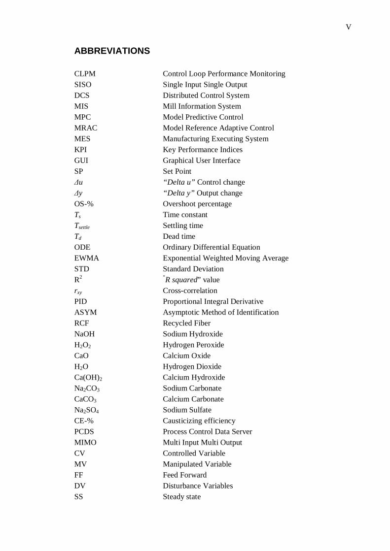
ABBREVIATIONS CLPM Control Loop Performance Monitoring SISO Single Input Single Output DCS Distributed Control System MIS Mill Information System MPC Model Predictive Control MRAC Model Reference Adaptive Control MES Manufacturing Executing System KPI Key Performance Indices GUI Graphical User Interface SP Set Point
u “Delta u” Control change y “Delta y” Output change
OS-% Overshoot percentage Ts Time constant Tsettle Settling time Td Dead time ODE Ordinary Differential Equation EWMA Exponential Weighted Moving Average STD Standard Deviation R2 “R squared” value rxy Cross-correlation PID Proportional Integral Derivative ASYM Asymptotic Method of Identification RCF Recycled Fiber NaOH Sodium Hydroxide H2O2 Hydrogen Peroxide CaO Calcium Oxide H2O Hydrogen Dioxide Ca(OH)2 Calcium Hydroxide Na2CO3 Sodium Carbonate CaCO3 Calcium Carbonate Na2SO4 Sodium Sulfate CE-% Causticizing efficiency PCDS Process Control Data Server MIMO Multi Input Multi Output CV Controlled Variable MV Manipulated Variable FF Feed Forward DV Disturbance Variables SS Steady state
VI
FPM First Principal Model ERIC Effective Residual Ink Concentration J Cost function e Control error
“Delta " Predicted control change LP Linear Programming QP Quadratic Programming DMC Dynamic Matrix Control OPC OLE for Process Control; OLE= Object Linking and Em-
bedding GL Green Liquor WL White Liquor TTA Total Titrative Alkali MRAS Model Reference Adaptive System NumPy Numerical Python MIT Massachusetts Institute of Technology VPN Virtual Private Network Kmodel coefficient Model coefficient MVhigh limit Manipulated variable high limit MVlow limit Manipulated variable low limit Kp Process gain CaCl2 Calcium chloride PV Process Value MM Model Mismatch IAE Integrated Average Error CO Controller Output
1
1 INTRODUCTION
Nowadays, in the pulp and paper industry one challenge is the continuous optimization of manufacturing processes in terms of production, quality and cost. Global competition combined with high costs of raw material as well as energy pricing are driving compa-nies to improve their process performance in order to reach their goals and meet end-user demands.
Most processes are multivariate, which means that there are more than one input and output variable that might all have a relationship with one another. A multivariate pro-cess requires an advanced control solution. An advanced control solution can manage several entities instead of single control loop. It is also unnecessary to try to control the-se kinds of processes manually. With the increased level of automation monitoring sys-tems are connected to more equipment and process more data at the same time. A mul-tivariate process also requires that a control engineer needs to be aware of more than one process variable at a time. A control loop performance monitoring (CLPM) pro-vides real time awareness of the process, thus allowing high process performance. The methods used for single input and single output processes are applicable for multivariate processes as well. Since there are more than one variable that needs to be considered of, process monitoring has to be evaluated differently. Lynch (1992) studied control loop performance monitoring for single input, single output (SISO) industrial processes, us-ing mathematical analysis methods and simulation. Studies regarding control loop per-formance monitoring usually include expert systems, pattern recognition, or quantative time-series analysis approaches (Kraus & Myron, 1984;Hägglund, 1992).
2
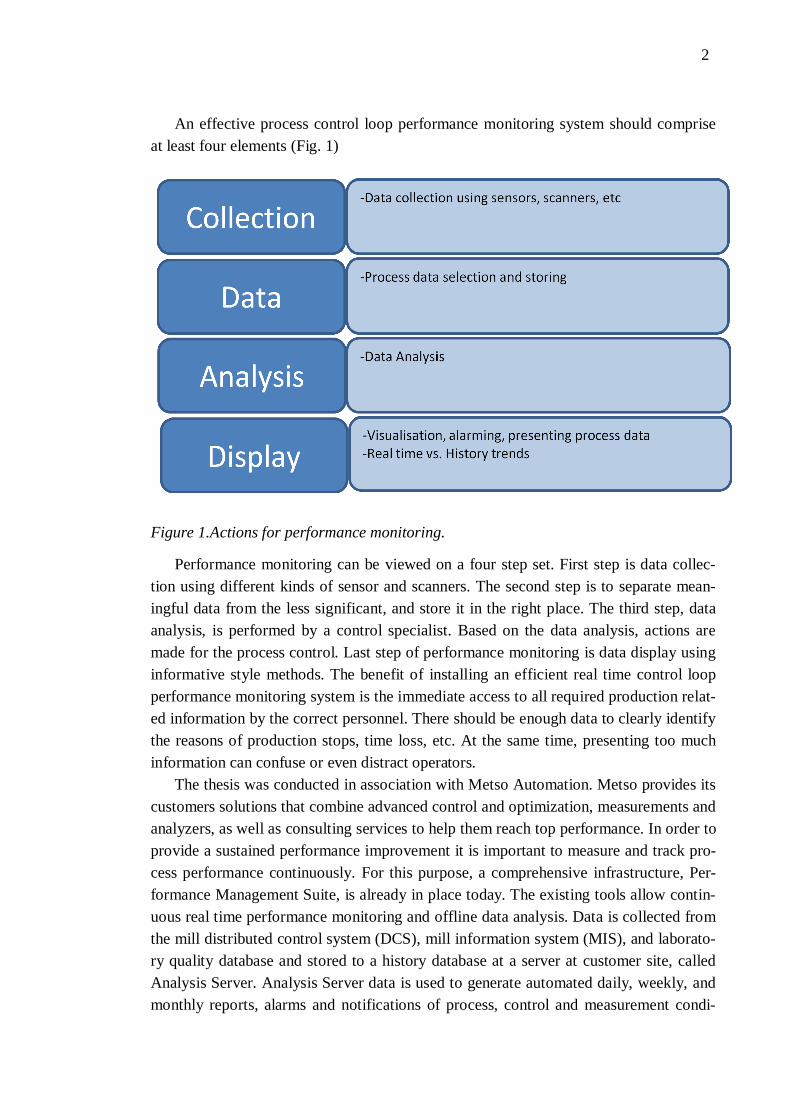
An effective process control loop performance monitoring system should comprise
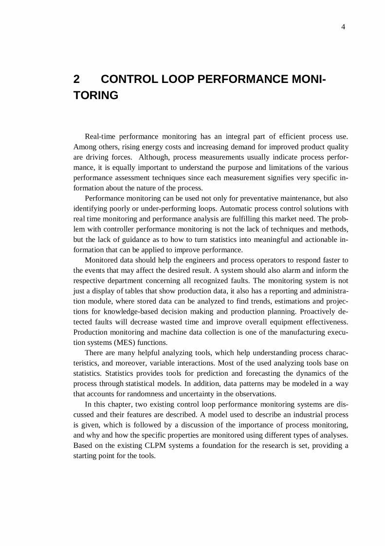
at least four elements (Fig. 1)
Figure 1.Actions for performance monitoring.
Performance monitoring can be viewed on a four step set. First step is data collec-tion using different kinds of sensor and scanners. The second step is to separate mean-ingful data from the less significant, and store it in the right place. The third step, data analysis, is performed by a control specialist. Based on the data analysis, actions are made for the process control. Last step of performance monitoring is data display using informative style methods. The benefit of installing an efficient real time control loop performance monitoring system is the immediate access to all required production relat-ed information by the correct personnel. There should be enough data to clearly identify the reasons of production stops, time loss, etc. At the same time, presenting too much information can confuse or even distract operators.
The thesis was conducted in association with Metso Automation. Metso provides its customers solutions that combine advanced control and optimization, measurements and analyzers, as well as consulting services to help them reach top performance. In order to provide a sustained performance improvement it is important to measure and track pro-cess performance continuously. For this purpose, a comprehensive infrastructure, Per-formance Management Suite, is already in place today. The existing tools allow contin-uous real time performance monitoring and offline data analysis. Data is collected from the mill distributed control system (DCS), mill information system (MIS), and laborato-ry quality database and stored to a history database at a server at customer site, called Analysis Server. Analysis Server data is used to generate automated daily, weekly, and monthly reports, alarms and notifications of process, control and measurement condi-
3
tions, and trends. Both Metso’s control specialists and customers are users of the Per-formance Management Suite. The Analysis Server is accessible for both local and re-mote users, which allows the specialists to provide off-site support for customers.
The aim of this thesis is to provide a solution that demonstrates controller perfor-mance effectively and informatively. The tools that are used today project the overall performance and final quality well but they fail to unveil the dependencies between pro-cess parameters. For complex, multivariate and highly interactive processes it is im-portant to understand these dependencies in order to achieve a highest possible control performance. The aim of this thesis is to find solutions for the following questions:
Which analysis method gives the most information of process state, and will
it provide a solution for effective performance monitoring? Which are the necessary key elements for indicating control performance?
Two control solutions, model predictive control (MPC) and model reference adap-
tive control (MRAC), were used as case examples for testing the selected study method. MPC is a control solution that predicts the change in the dependent variables of the modeled systems caused by changes in the independent variables. The use of MPC started to increase in 1970’s (Richalet et al 1978; Cutler & Ramaker 1979) in the petro-chemical industry. MRAC is a control solution, where the closed system output at-tempts to follow a given process model. Whitaker studied the design of MRAC for air-craft control already in 1959 (Whitaker 1959).
In this thesis, mathematical and statistical analyzing methods combined with visual analyses were used as study methods to detect how the controller is performing. Based on the study, an intelligent control loop performance monitoring tools for both of the control solutions were implemented. The implemented control loop performance moni-toring tools were applied to ongoing processes, thus giving a more realistic outcome. The tool is primarily targeted for Metso’s control specialists. A control loop perfor-mance monitoring software can also perform as a major asset guiding a young engineer through the process control interactions as well as providing a useful tool for training.
This thesis work is structured so that public domain information of the commercially available solutions is studied in chapter 2. In chapter 3 the studied processes are intro-duced. Chapters 4 and 5 focus on the concepts of the two control methods. Conclusions made based on the public domain information in chapter 2 and the review of process requirements in chapters 3 to 5, will guideline the implementation of the intelligent con-trol loop performance monitoring solution design. Design and implementation of the intelligent monitoring application for MPC and MRAC is described in chapter 6. Final-ly, chapter 7 reviews the achieved results and discusses the future work for improving the performance tools.
4
2 CONTROL LOOP PERFORMANCE MONI-TORING
Real-time performance monitoring has an integral part of efficient process use. Among others, rising energy costs and increasing demand for improved product quality are driving forces. Although, process measurements usually indicate process perfor-mance, it is equally important to understand the purpose and limitations of the various performance assessment techniques since each measurement signifies very specific in-formation about the nature of the process.
Performance monitoring can be used not only for preventative maintenance, but also identifying poorly or under-performing loops. Automatic process control solutions with real time monitoring and performance analysis are fulfilling this market need. The prob-lem with controller performance monitoring is not the lack of techniques and methods, but the lack of guidance as to how to turn statistics into meaningful and actionable in-formation that can be applied to improve performance.
Monitored data should help the engineers and process operators to respond faster to the events that may affect the desired result. A system should also alarm and inform the respective department concerning all recognized faults. The monitoring system is not just a display of tables that show production data, it also has a reporting and administra-tion module, where stored data can be analyzed to find trends, estimations and projec-tions for knowledge-based decision making and production planning. Proactively de-tected faults will decrease wasted time and improve overall equipment effectiveness. Production monitoring and machine data collection is one of the manufacturing execu-tion systems (MES) functions.
There are many helpful analyzing tools, which help understanding process charac-teristics, and moreover, variable interactions. Most of the used analyzing tools base on statistics. Statistics provides tools for prediction and forecasting the dynamics of the process through statistical models. In addition, data patterns may be modeled in a way that accounts for randomness and uncertainty in the observations.
In this chapter, two existing control loop performance monitoring systems are dis-cussed and their features are described. A model used to describe an industrial process is given, which is followed by a discussion of the importance of process monitoring, and why and how the specific properties are monitored using different types of analyses. Based on the existing CLPM systems a foundation for the research is set, providing a starting point for the tools.
5
2.1 Process Monitoring, Fault Detections and Diagnos-tics
Fault diagnosis has a primary importance in modern process automation. It provides the bases for fault tolerance, reliability or security, which constitutes fundamental de-sign features in complex engineering systems. The system under consideration is moni-tored and the data is passed to fault detection algorithms or procedures. The most basic form of fault detection is to register an alarm when an abnormal condition develops in the monitored system. Once a fault is detected, procedures may also be used to identify or diagnose the cause of the abnormal situation. Comparing the monitored data to previ-ous estimates will provide a good evaluation of model quality. If there are inconsisten-cies, it might be an indication that at least one fault has occurred. Detecting the faults and their causes, thus making adjustments to the process models is crucial preparing for future exceptions.
2.2 Benefits of Control Loop Performance Monitoring
There are multiple benefits for implementing a control loop performance monitoring (CLPM) software, and it is helpful for both the control system provider as well as the customer. First, CLPM software provides the engineers and technicians a tool to identi-fy the good and poor performing control loops. Further analysis allows diagnostics for the causes of poorly performing control loops. A control loop may be performing poor-ly, but if it is not an important control loop it can be ignored if higher prioritized control loops are performing poorly as well. CLPM software considers both the performance and the importance of control loops, process control tuning work can be prioritized, thus improving work efficiency and save time.
A control loop performance monitoring software can maintain history on several as-pects of control loop performance and controller tuning settings. These can be trended over time to see the effect of tuning changes on loop performance. It is helpful to see at what point in time the tuning settings were changed, what the old values were, what they were changed to, and what effect the changes had on for example loop perfor-mance.
An essential aspect of any performance improvement initiative is the reporting and monitoring of key performance indicators (KPI’s). A KPI is a type of measurement, which in process industry can be e.g. a guaranteed process value improvement due to the installed control solution. The parameters produced by CLPM software can be use-ful for evaluating the success of a control optimization project or loop tuning effort through a before and after comparison. CLPM software not only indicates which loops have poor performance, but also gives a diagnosis of why the performance is poor. Off-tuning, oscillations, and controller output running into limits are examples of diagnos-tics which the software can present.
6
2.3 Process Characteristics Analysis
All processes have some kind of variation. Without variation there would be no need for control engineering. Process variable interactions cause one part of the variation and some of the variation is due to natural process variation or noise. Data collection and visualization is crucial part of process monitoring but to actually improving the process and evaluate its characteristics, it is important to have powerful analyzing tools.
2.3.1 Interactive Visual Analysis
Interactive visual analysis combines a computer with the perceptive capabilities of humans, in order to extract knowledge from large and complex datasets. This analysis method relies heavily on graphical user interface (GUI), usually provided by computers. Interactive visual analysis well suited for analyzing high-dimensional data that has a large number of data points, where simple graphing and non-interactive techniques give an insufficient understanding of the information.
2.3.2 Set Point Analysis
Set point (SP) analysis is made by executing a step-response test. In a step-response test, a change is made in an input variable u, which causes a certain change in an out-put variable y. There are a number of techniques for analyzing closed loop process data that is collected during a set point response experiment. These techniques allow an orderly comparison of process response shapes and characteristics. When analyzing a set point response, the criteria used to describe how well the process responds to the change can include for example process overshoot (OS-%), rise time and settling time.
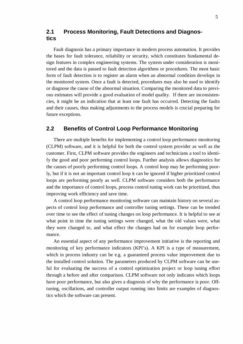
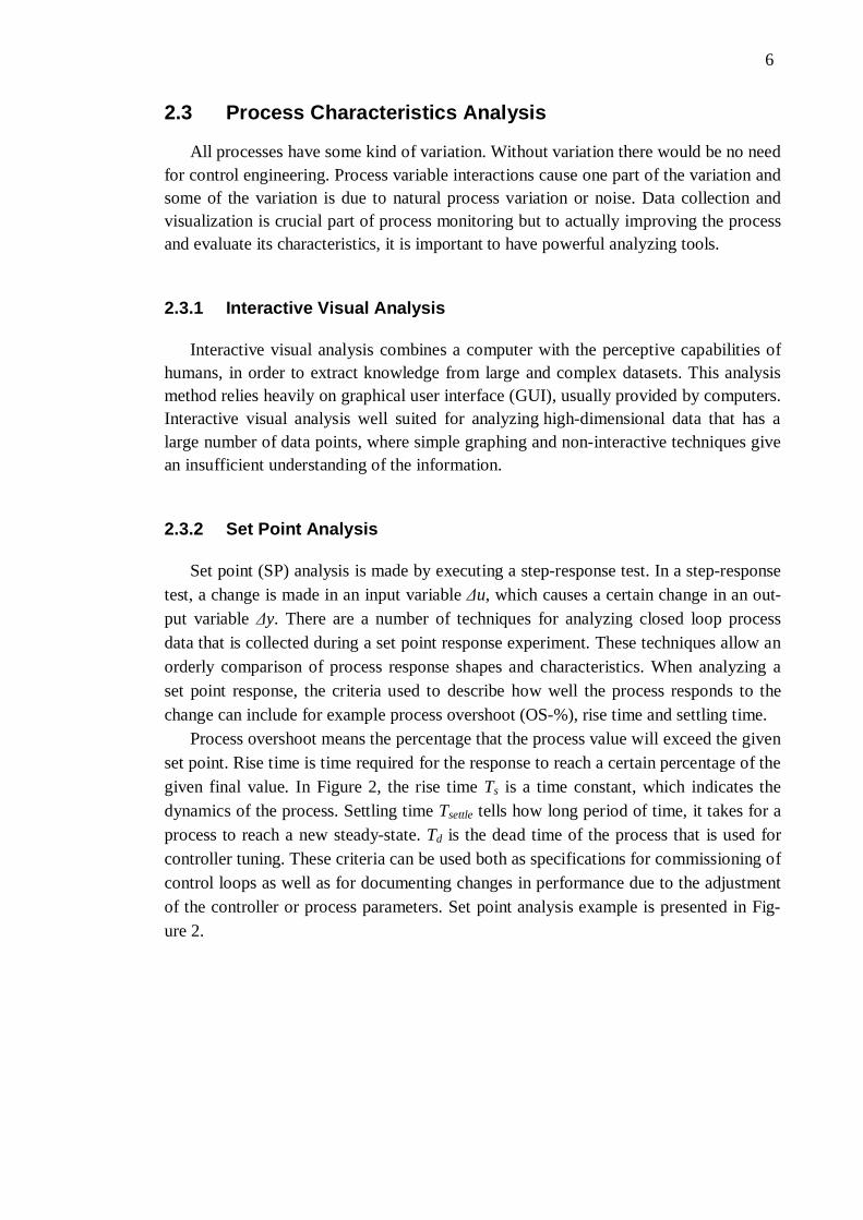
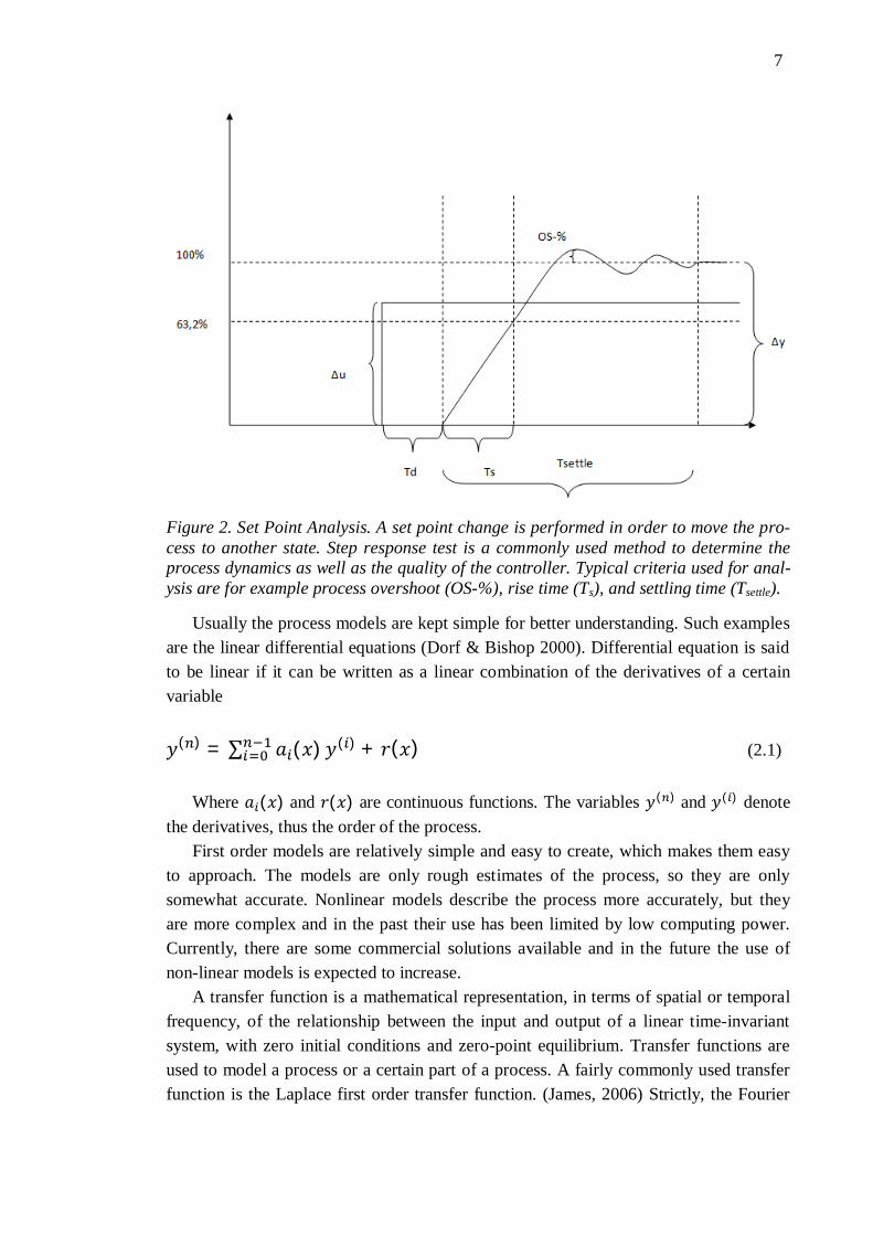
Process overshoot means the percentage that the process value will exceed the given set point. Rise time is time required for the response to reach a certain percentage of the given final value. In Figure 2, the rise time Ts is a time constant, which indicates the dynamics of the process. Settling time Tsettle tells how long period of time, it takes for a process to reach a new steady-state. Td is the dead time of the process that is used for controller tuning. These criteria can be used both as specifications for commissioning of control loops as well as for documenting changes in performance due to the adjustment of the controller or process parameters. Set point analysis example is presented in Fig-ure 2.
7
Figure 2. Set Point Analysis. A set point change is performed in order to move the pro-cess to another state. Step response test is a commonly used method to determine the process dynamics as well as the quality of the controller. Typical criteria used for anal-ysis are for example process overshoot (OS-%), rise time (Ts), and settling time (Tsettle).
Usually the process models are kept simple for better understanding. Such examples are the linear differential equations (Dorf & Bishop 2000). Differential equation is said to be linear if it can be written as a linear combination of the derivatives of a certain variable
( ) = ( ) ( ) + ( ) (2.1)
Where ( ) and ( ) are continuous functions. The variables ( ) and ( ) denote
the derivatives, thus the order of the process. First order models are relatively simple and easy to create, which makes them easy
to approach. The models are only rough estimates of the process, so they are only somewhat accurate. Nonlinear models describe the process more accurately, but they are more complex and in the past their use has been limited by low computing power. Currently, there are some commercial solutions available and in the future the use of non-linear models is expected to increase.
A transfer function is a mathematical representation, in terms of spatial or temporal frequency, of the relationship between the input and output of a linear time-invariant system, with zero initial conditions and zero-point equilibrium. Transfer functions are used to model a process or a certain part of a process. A fairly commonly used transfer function is the Laplace first order transfer function. (James, 2006) Strictly, the Fourier
8
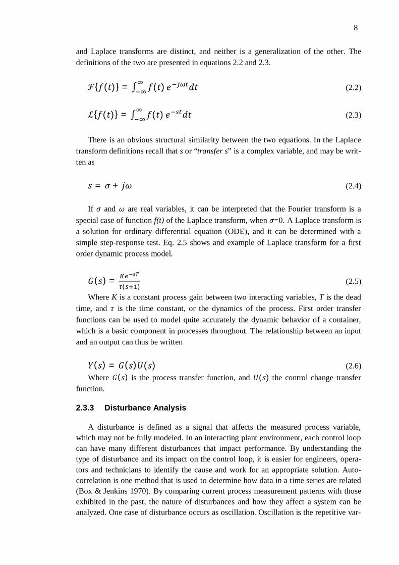
and Laplace transforms are distinct, and neither is a generalization of the other. The definitions of the two are presented in equations 2.2 and 2.3.
{ ( )} = ( ) (2.2)
{ ( )} = ( ) (2.3)
There is an obvious structural similarity between the two equations. In the Laplace
transform definitions recall that s or “transfer s” is a complex variable, and may be writ-ten as
= + (2.4)
If and are real variables, it can be interpreted that the Fourier transform is a
special case of function f(t) of the Laplace transform, when =0. A Laplace transform is a solution for ordinary differential equation (ODE), and it can be determined with a simple step-response test. Eq. 2.5 shows and example of Laplace transform for a first order dynamic process model.
( ) =( )
(2.5)
Where K is a constant process gain between two interacting variables, T is the dead time, and is the time constant, or the dynamics of the process. First order transfer functions can be used to model quite accurately the dynamic behavior of a container, which is a basic component in processes throughout. The relationship between an input and an output can thus be written
( ) = ( ) ( ) (2.6)
Where ( ) is the process transfer function, and ( ) the control change transfer function.
2.3.3 Disturbance Analysis
A disturbance is defined as a signal that affects the measured process variable, which may not be fully modeled. In an interacting plant environment, each control loop can have many different disturbances that impact performance. By understanding the type of disturbance and its impact on the control loop, it is easier for engineers, opera-tors and technicians to identify the cause and work for an appropriate solution. Auto-correlation is one method that is used to determine how data in a time series are related (Box & Jenkins 1970). By comparing current process measurement patterns with those exhibited in the past, the nature of disturbances and how they affect a system can be analyzed. One case of disturbance occurs as oscillation. Oscillation is the repetitive var-
9
iation, typically in time, of some measure about a central or between two or more dif-ferent states. Oscillation is used not only to determine a disturbance, but also find the source variable of process variation.
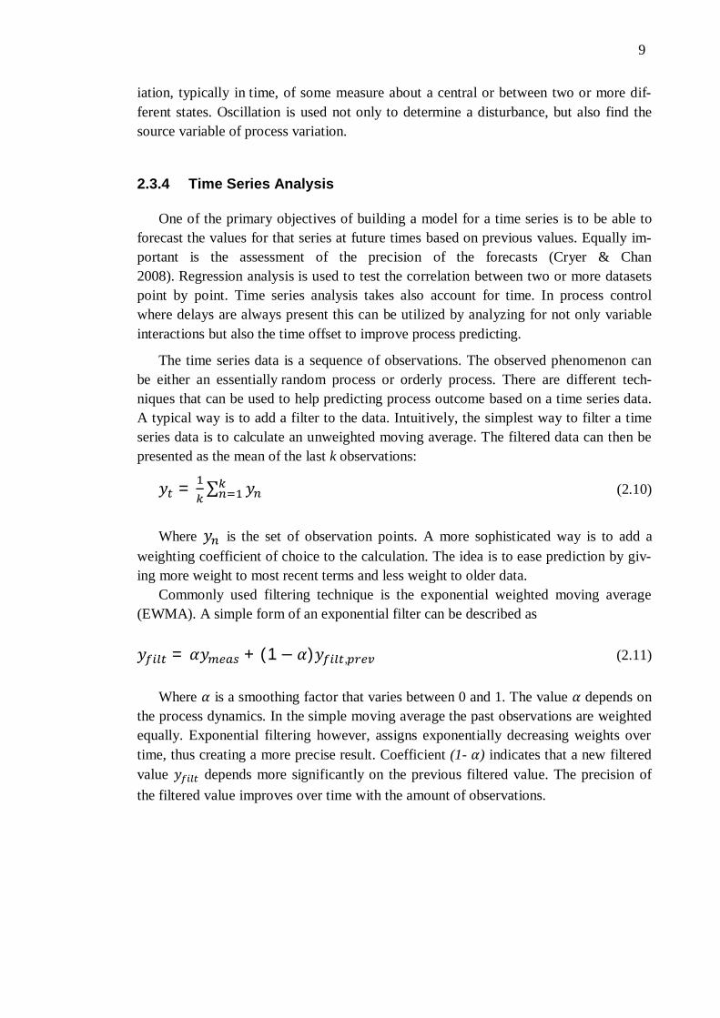
2.3.4 Time Series Analysis
One of the primary objectives of building a model for a time series is to be able to forecast the values for that series at future times based on previous values. Equally im-portant is the assessment of the precision of the forecasts (Cryer & Chan 2008). Regression analysis is used to test the correlation between two or more datasets point by point. Time series analysis takes also account for time. In process control where delays are always present this can be utilized by analyzing for not only variable interactions but also the time offset to improve process predicting.
The time series data is a sequence of observations. The observed phenomenon can be either an essentially random process or orderly process. There are different tech-niques that can be used to help predicting process outcome based on a time series data. A typical way is to add a filter to the data. Intuitively, the simplest way to filter a time series data is to calculate an unweighted moving average. The filtered data can then be presented as the mean of the last k observations:
= (2.10)
Where is the set of observation points. A more sophisticated way is to add a
weighting coefficient of choice to the calculation. The idea is to ease prediction by giv-ing more weight to most recent terms and less weight to older data.
Commonly used filtering technique is the exponential weighted moving average (EWMA). A simple form of an exponential filter can be described as
= + (1 ) , (2.11)
Where is a smoothing factor that varies between 0 and 1. The value depends on
the process dynamics. In the simple moving average the past observations are weighted equally. Exponential filtering however, assigns exponentially decreasing weights over time, thus creating a more precise result. Coefficient (1- ) indicates that a new filtered value depends more significantly on the previous filtered value. The precision of the filtered value improves over time with the amount of observations.
10
2.3.5 Bi-variate Regression and Correlation Analysis
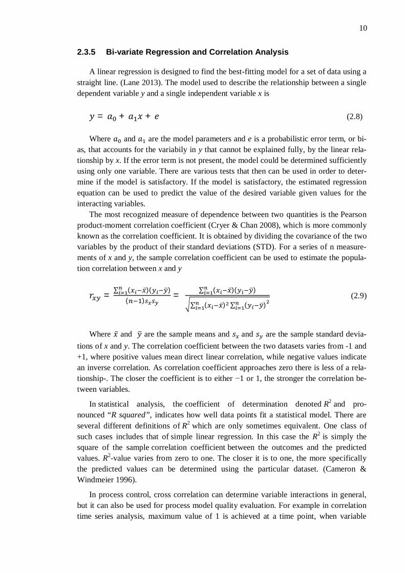
A linear regression is designed to find the best-fitting model for a set of data using a straight line. (Lane 2013). The model used to describe the relationship between a single dependent variable y and a single independent variable x is
= + + (2.8)
Where and are the model parameters and e is a probabilistic error term, or bi-
as, that accounts for the variabily in y that cannot be explained fully, by the linear rela-tionship by x. If the error term is not present, the model could be determined sufficiently using only one variable. There are various tests that then can be used in order to deter-mine if the model is satisfactory. If the model is satisfactory, the estimated regression equation can be used to predict the value of the desired variable given values for the interacting variables.
The most recognized measure of dependence between two quantities is the Pearson product-moment correlation coefficient (Cryer & Chan 2008), which is more commonly known as the correlation coefficient. It is obtained by dividing the covariance of the two variables by the product of their standard deviations (STD). For a series of n measure-ments of x and y, the sample correlation coefficient can be used to estimate the popula-tion correlation between x and y
= ( )( )( ) = ( )( )
( ) ( ) (2.9)
Where and are the sample means and and are the sample standard devia-tions of x and y. The correlation coefficient between the two datasets varies from -1 and +1, where positive values mean direct linear correlation, while negative values indicate an inverse correlation. As correlation coefficient approaches zero there is less of a rela-tionship-. The closer the coefficient is to either 1 or 1, the stronger the correlation be-tween variables.
In statistical analysis, the coefficient of determination denoted R2 and pro-nounced “R squared”, indicates how well data points fit a statistical model. There are several different definitions of R2 which are only sometimes equivalent. One class of such cases includes that of simple linear regression. In this case the R2 is simply the square of the sample correlation coefficient between the outcomes and the predicted values. R2-value varies from zero to one. The closer it is to one, the more specifically the predicted values can be determined using the particular dataset. (Cameron & Windmeier 1996).
In process control, cross correlation can determine variable interactions in general, but it can also be used for process model quality evaluation. For example in correlation time series analysis, maximum value of 1 is achieved at a time point, when variable
11
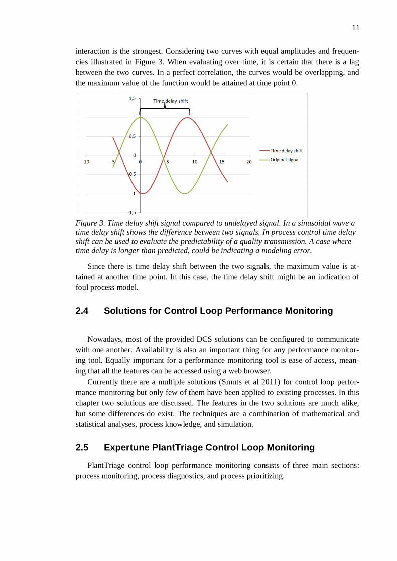
interaction is the strongest. Considering two curves with equal amplitudes and frequen-cies illustrated in Figure 3. When evaluating over time, it is certain that there is a lag between the two curves. In a perfect correlation, the curves would be overlapping, and the maximum value of the function would be attained at time point 0.
Figure 3. Time delay shift signal compared to undelayed signal. In a sinusoidal wave a time delay shift shows the difference between two signals. In process control time delay shift can be used to evaluate the predictability of a quality transmission. A case where time delay is longer than predicted, could be indicating a modeling error.
Since there is time delay shift between the two signals, the maximum value is at-tained at another time point. In this case, the time delay shift might be an indication of foul process model.
2.4 Solutions for Control Loop Performance Monitoring
Nowadays, most of the provided DCS solutions can be configured to communicate
with one another. Availability is also an important thing for any performance monitor-ing tool. Equally important for a performance monitoring tool is ease of access, mean-ing that all the features can be accessed using a web browser.
Currently there are a multiple solutions (Smuts et al 2011) for control loop perfor-mance monitoring but only few of them have been applied to existing processes. In this chapter two solutions are discussed. The features in the two solutions are much alike, but some differences do exist. The techniques are a combination of mathematical and statistical analyses, process knowledge, and simulation.
2.5 Expertune PlantTriage Control Loop Monitoring
PlantTriage control loop performance monitoring consists of three main sections: process monitoring, process diagnostics, and process prioritizing.
12
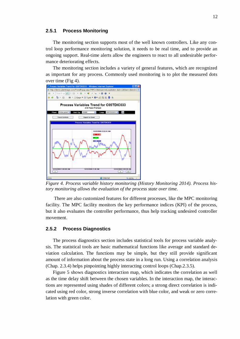
2.5.1 Process Monitoring
The monitoring section supports most of the well known controllers. Like any con-trol loop performance monitoring solution, it needs to be real time, and to provide an ongoing support. Real-time alerts allow the engineers to react to all undesirable perfor-mance deteriorating effects.
The monitoring section includes a variety of general features, which are recognized as important for any process. Commonly used monitoring is to plot the measured dots over time (Fig 4).
Figure 4. Process variable history monitoring (History Monitoring 2014). Process his-tory monitoring allows the evaluation of the process state over time.
There are also customized features for different processes, like the MPC monitoring facility. The MPC facility monitors the key performance indices (KPI) of the process, but it also evaluates the controller performance, thus help tracking undesired controller movement.
2.5.2 Process Diagnostics
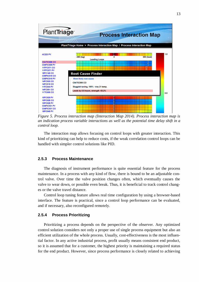
The process diagnostics section includes statistical tools for process variable analy-sis. The statistical tools are basic mathematical functions like average and standard de-viation calculation. The functions may be simple, but they still provide significant amount of information about the process state in a long run. Using a correlation analysis (Chap. 2.3.4) helps pinpointing highly interacting control loops (Chap.2.3.5).
Figure 5 shows diagnostics interaction map, which indicates the correlation as well as the time delay shift between the chosen variables. In the interaction map, the interac-tions are represented using shades of different colors; a strong direct correlation is indi-cated using red color, strong inverse correlation with blue color, and weak or zero corre-lation with green color.
13
Figure 5. Process interaction map (Interaction Map 2014). Process interaction map is an indication process variable interactions as well as the potential time delay shift in a control loop.
The interaction map allows focusing on control loops with greater interaction. This kind of prioritizing can help to reduce costs, if the weak correlation control loops can be handled with simpler control solutions like PID.
2.5.3 Process Maintenance
The diagnosis of instrument performance is quite essential feature for the process maintenance. In a process with any kind of flow, there is bound to be an adjustable con-trol valve. Over time the valve position changes often, which eventually causes the valve to wear down, or possible even break. Thus, it is beneficial to track control chang-es or the valve travel distance.
Control loop tuning feature allows real time configuration by using a browser-based interface. The feature is practical, since a control loop performance can be evaluated, and if necessary, also reconfigured remotely.
2.5.4 Process Prioritizing
Prioritizing a process depends on the perspective of the observer. Any optimized control solution considers not only a proper use of single process equipment but also an efficient utilization of the whole process. Usually, cost-effectiveness is the most influen-tial factor. In any active industrial process, profit usually means consistent end product, so it is assumed that for a customer, the highest priority is maintaining a required status for the end product. However, since process performance is closely related to achieving
14
a desired end profit value, it is equally important to detect poorly performing control loops as well as the biggest payback loops.
2.6 Control Performance Monitor by Matrikon
As well as the control loop performance monitoring system by Expertune, the Con-trol Performance Monitor by Matrikon is an independent solution, meaning that it can be applied as a part of a control system. The features are much alike the ones in Expertune.
2.6.1 Process Monitoring
As mentioned, trending a process variable over time is commonly used monitoring procedure. It will help to get a rough estimate of the current state as well as the progress of the process. Statistical analysis methods help not only identifying process difficulties but can also be used for monitoring purposes as well.
2.6.2 Process Identification
For process modeling and control loop tuning, the Expertune performance monitor-ing solution had a PID control loop tuning feature, which was accessible remotely in any standard web browser, and had the ability to be configured online. The Control Per-formance Monitor has the same feature, but unlike in PlantTriage, where the process was modeled using individual step response test, Control Performance Monitor uses the TaiJi process modeling technology, where more than one step tests are performed sim-ultaneously.The method was originally developed for single variable processes by Ljung and Yuan in 1985, and extended later for multivariate cases (Zhu 1989).
2.7 Optimal Process Performance Monitoring
Classification of real time information helps understanding how the desired monitor-ing system should be structured. The idea of a real time monitoring system is not to give some information simultaneously with the event but to provide the production team, as fast as possible, with the accurate and meaningful data. But there should be enough time to respond timely on these events. It will always take some time, sometimes even hours, to analyze monitored data and to respond to it. There are many different techniques and methods to analyze existing data, both online and offline. Some rely solely on statistics while others are more process knowledge based. An optimum solution takes account for both statistical and intuitive approaches. It is important to be aware of that neither one of two always provides the best possible solution.
Process performance is not only an indication of the process status but also the con-trol solution. Regardless of the point of view, process performance needs to be moni-tored informatively, and the presentation should be easily understood. The right kind of well presented performance information will provide a feasible outcome.
15
3 PROCESS INTRODUCTION
3.1 Recycled Fiber Process
Paper recycling is the process of converting waste paper into new paper products. Large variations in the raw material quality and composition are typical for the recycled fibers processes due to the diversity of the raw material. Besides contaminants, recov-ered paper always contains varying amount of fillers and coating pigments. Recycled Fiber (RCF) processing must therefore accommodate changes of the furnish quality. (Holik 2000)
The complexity of the process makes it a challenging subject for control. For com-plex multivariate processes a modern control solution like Model Predictive Control (MPC) is required. The complexity of the RCF process is based on two issues, when comparing to virgin fiber manufacturing processes. First, the recovered pulp contains more than one type of fiber or paper grades. More importantly, it also contains different contaminants and substances such as fillers, coating components, printing inks, and ad-hesives. For mechanical and optical characteristics it is necessary for a RCF process to meet the requirements when it comes to fiber quality and cleanliness. Selection and monitoring of RCF play important roles in making the RCF process cost-efficient and maintaining adequate quality of the finished product. The primary tasks of RCF process are contaminant removal and eliminating their effects in order to meet the quality re-quirements. The desired savings can be achieved by monitoring proactively the entire process from pulper to paper machine.
The industrial process of removing printing ink from paper fibers of recycled pa-per is called deinking. In particular, change in the ratio between newsprint and maga-zine affects the deinking process directly. The ash and filler content, yield as well as foaming ability, affect significantly on brightness, consistency, and strength properties. (Holik 2000). Deinking requires utilizing both chemical and mechanical techniques. The process has multiple interactive handles that affect final quality. To contribute the suc-cess of deinking, the process is divided into sub processes: pulping, screening, cleaning, pre- and post-flotation, dispersion, and bleaching.
Pulping The first step of the deinking process is to disintegrate the waste paper in water at
relatively low consistency (5-18%), which is called pulping. Consistency is an im-portant quality for chemical dosages, since a higher stock consistency in a pulper means less water and a higher concentration of chemicals. Chemicals are used to contribute the disintegration of fibers. Pulping is one of the key components affecting process perfor-
16
mance and efficiency of RCF. The process consists of feeder, pulper, and reject screen-ing. The feeding equipment structure is determined by the raw material. Similarly, pulp-ing can be done in pulpers or drum pulpers depending on the condition of the feed raw material.
In the pulping stage, the pH of the stock is increased with caustic soda, also known as Sodium Hydroxide (NaOH), to as high as approximately 9-10. Caustic soda is added to swell the fibers, so that the printing ink can be removed easily.
The Hydrogen Peroxide (H2O2) is added to the pulper as a bleaching agent to reduce yellowing of the fibers caused by the caustic. Peroxide bleaching is also used in chemi-cal pulp production and is most successful at high temperature and consistency. On the other hand, high temperature softens the thermoplastic stickies that occur in recovered paper as contaminants and makes their removal more difficult. Soap is also added in pulping stage and it is used as a collector chemical. (Lassus 2000)
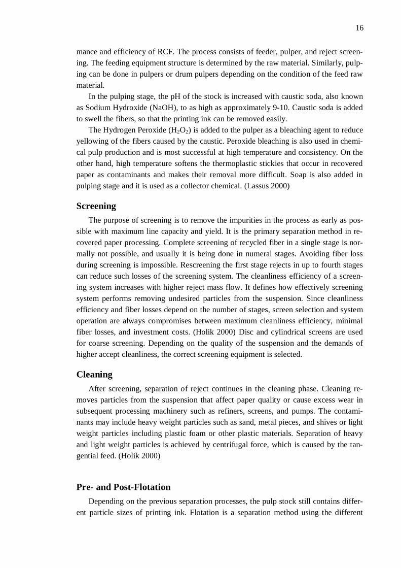
Screening The purpose of screening is to remove the impurities in the process as early as pos-
sible with maximum line capacity and yield. It is the primary separation method in re-covered paper processing. Complete screening of recycled fiber in a single stage is nor-mally not possible, and usually it is being done in numeral stages. Avoiding fiber loss during screening is impossible. Rescreening the first stage rejects in up to fourth stages can reduce such losses of the screening system. The cleanliness efficiency of a screen-ing system increases with higher reject mass flow. It defines how effectively screening system performs removing undesired particles from the suspension. Since cleanliness efficiency and fiber losses depend on the number of stages, screen selection and system operation are always compromises between maximum cleanliness efficiency, minimal fiber losses, and investment costs. (Holik 2000) Disc and cylindrical screens are used for coarse screening. Depending on the quality of the suspension and the demands of higher accept cleanliness, the correct screening equipment is selected.
Cleaning After screening, separation of reject continues in the cleaning phase. Cleaning re-
moves particles from the suspension that affect paper quality or cause excess wear in subsequent processing machinery such as refiners, screens, and pumps. The contami-nants may include heavy weight particles such as sand, metal pieces, and shives or light weight particles including plastic foam or other plastic materials. Separation of heavy and light weight particles is achieved by centrifugal force, which is caused by the tan-gential feed. (Holik 2000)
Pre- and Post-Flotation Depending on the previous separation processes, the pulp stock still contains differ-
ent particle sizes of printing ink. Flotation is a separation method using the different
17
surface properties of particles. In flotation process, air is introduced into a diluted fiber suspension. The hydrophobic or water-repelling ink particles attach to the air bubbles and rise to the surface, forming a layer of foam. Besides ink, the process also removes ash and fines from the suspension. The foam can be removed mechanically, by over-flow, or by a vacuum extraction.
The existing technologies vary widely, primarily by the aeration system, which can either be air-permeable bodies or static and dynamic mixers. Other variable features of flotation cells are the number of aeration stages and units required for complete flota-tion, air supply type, foam removal methods, closed or open cells, and cell design and arrangement of multiple cell units. (Lassus 2000) There is usually more than one section of flotation processes, regarding the different grades of fineness. A flotation process before dispersing is called pre-flotation, and after the disperser, it is called post-flotation.
Dispersion Dispersion involves application of high shear forces to the fibers and the debris par-
ticles to be dispersed. The stock is thickened so that the required amount of energy can be transferred.
In deinking process there are always dirt spots, coating particles, and ink that cannot be fully removed from the suspension. However, they can be grinded into almost invisi-ble pieces with dispersion process. Larger particles can be removed in a post-flotation or in an additional washing phase.
Dispersion process slightly decreases the brightness of the stock; at the same time the reduction of particle diminishes their re-flocculation at the paper machine, which furthermore enhances runnability on a paper or cardboard machine. Grinding treats fi-bers mechanically for retaining or improving their strength characteristics. Heat treat-ment of the heating screw also increases the fibers bulk properties. Bleaching chemicals can be added already on the disperser, when it can be treated as a mixing chamber. After dispersion, the stock is transported to a bleaching tower. (Holik 2000)
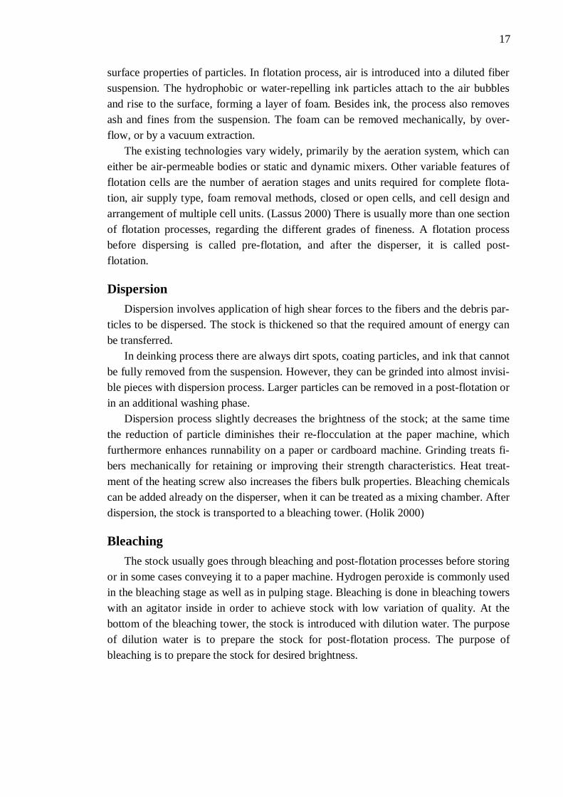
Bleaching The stock usually goes through bleaching and post-flotation processes before storing
or in some cases conveying it to a paper machine. Hydrogen peroxide is commonly used in the bleaching stage as well as in pulping stage. Bleaching is done in bleaching towers with an agitator inside in order to achieve stock with low variation of quality. At the bottom of the bleaching tower, the stock is introduced with dilution water. The purpose of dilution water is to prepare the stock for post-flotation process. The purpose of bleaching is to prepare the stock for desired brightness.
18
3.2 Causticizing Process
The target for causticizing process is to convert the inactive sodium carbonate (Na2CO3) into the active cooking chemical, sodium hydroxide (NaOH), as efficiently as possible. The process is usually divided into six unit operations: dissolving of molten smelt to produce green liquor, treatment of green liquor, slaking of lime, causticizing chambers, white liquor clarification, and lime mud dewatering.
Dissolving and Green Liquor Treatment Combustion of black liquor in recovery boiler produces inorganic chemical sub-
stances (Na2CO3 and Na2SO4) which form a molten bed on the bottom of the boiler. The smelt is then mixed with diluted weak white liquor, and the solution is called green liq-uor. The formed lime mud is filtered from the green liquor, and then washed with water. The resulting filtrate is weak white liquor, which then can be reused.
The basic purpose of green liquor treatment is to make the green liquor coming from the dissolver into a proper feed for causticizing. The treatment consists of removing solid impurities from the liquor, adjusting the temperature, and stabilizing system flow and fluctuations (Arpalahti et al. 2002).
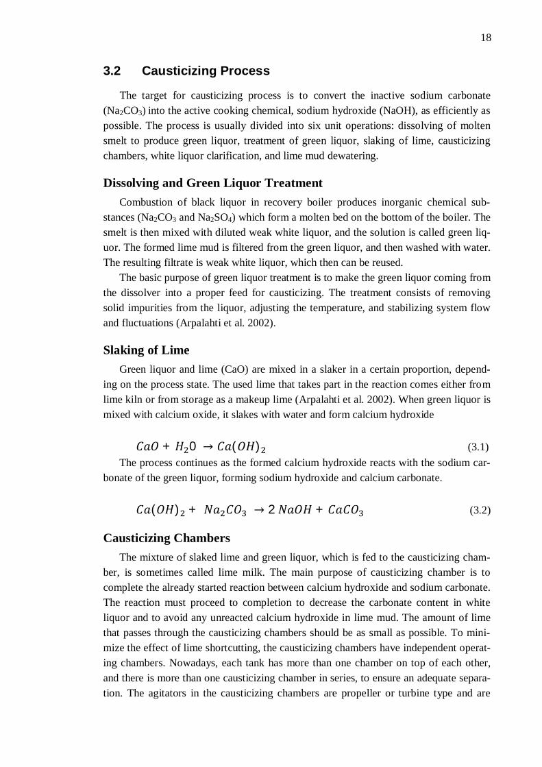
Slaking of Lime Green liquor and lime (CaO) are mixed in a slaker in a certain proportion, depend-
ing on the process state. The used lime that takes part in the reaction comes either from lime kiln or from storage as a makeup lime (Arpalahti et al. 2002). When green liquor is mixed with calcium oxide, it slakes with water and form calcium hydroxide
+ 0 ( ) (3.1)
The process continues as the formed calcium hydroxide reacts with the sodium car-bonate of the green liquor, forming sodium hydroxide and calcium carbonate.
( ) + 2 + (3.2)
Causticizing Chambers The mixture of slaked lime and green liquor, which is fed to the causticizing cham-
ber, is sometimes called lime milk. The main purpose of causticizing chamber is to complete the already started reaction between calcium hydroxide and sodium carbonate. The reaction must proceed to completion to decrease the carbonate content in white liquor and to avoid any unreacted calcium hydroxide in lime mud. The amount of lime that passes through the causticizing chambers should be as small as possible. To mini-mize the effect of lime shortcutting, the causticizing chambers have independent operat-ing chambers. Nowadays, each tank has more than one chamber on top of each other, and there is more than one causticizing chamber in series, to ensure an adequate separa-tion. The agitators in the causticizing chambers are propeller or turbine type and are
19
used to improve mixing, thus enhancing the completion of the reaction. (Arpalahti et al. 2002)
The degree of causticizing, or causticizing efficiency (CE-%), describes the com-pleteness of the reaction at equilibrium. Typically, the degree of causticizing is around 70-80%, depending on concentration and sulfidity level.
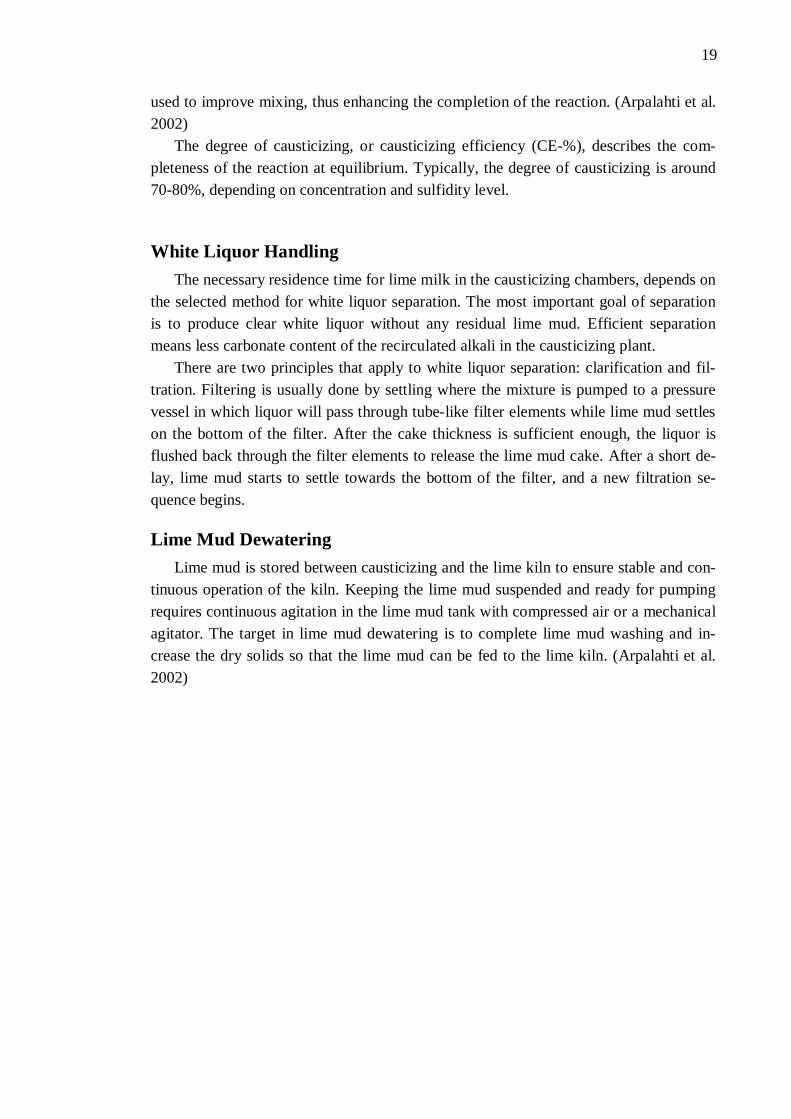
White Liquor Handling The necessary residence time for lime milk in the causticizing chambers, depends on
the selected method for white liquor separation. The most important goal of separation is to produce clear white liquor without any residual lime mud. Efficient separation means less carbonate content of the recirculated alkali in the causticizing plant.
There are two principles that apply to white liquor separation: clarification and fil-tration. Filtering is usually done by settling where the mixture is pumped to a pressure vessel in which liquor will pass through tube-like filter elements while lime mud settles on the bottom of the filter. After the cake thickness is sufficient enough, the liquor is flushed back through the filter elements to release the lime mud cake. After a short de-lay, lime mud starts to settle towards the bottom of the filter, and a new filtration se-quence begins.
Lime Mud Dewatering Lime mud is stored between causticizing and the lime kiln to ensure stable and con-
tinuous operation of the kiln. Keeping the lime mud suspended and ready for pumping requires continuous agitation in the lime mud tank with compressed air or a mechanical agitator. The target in lime mud dewatering is to complete lime mud washing and in-crease the dry solids so that the lime mud can be fed to the lime kiln. (Arpalahti et al. 2002)
20
4 RECYCLED FIBER DEINKING PROCESS CONTROL
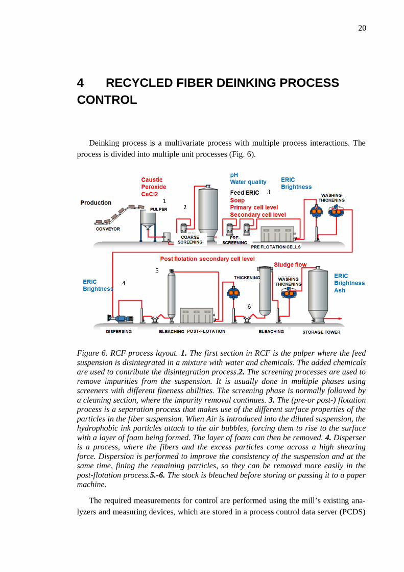
Deinking process is a multivariate process with multiple process interactions. The process is divided into multiple unit processes (Fig. 6).
Figure 6. RCF process layout. 1. The first section in RCF is the pulper where the feed suspension is disintegrated in a mixture with water and chemicals. The added chemicals are used to contribute the disintegration process.2. The screening processes are used to remove impurities from the suspension. It is usually done in multiple phases using screeners with different fineness abilities. The screening phase is normally followed by a cleaning section, where the impurity removal continues. 3. The (pre-or post-) flotation process is a separation process that makes use of the different surface properties of the particles in the fiber suspension. When Air is introduced into the diluted suspension, the hydrophobic ink particles attach to the air bubbles, forcing them to rise to the surface with a layer of foam being formed. The layer of foam can then be removed. 4. Disperser is a process, where the fibers and the excess particles come across a high shearing force. Dispersion is performed to improve the consistency of the suspension and at the same time, fining the remaining particles, so they can be removed more easily in the post-flotation process.5.-6. The stock is bleached before storing or passing it to a paper machine.
The required measurements for control are performed using the mill’s existing ana-lyzers and measuring devices, which are stored in a process control data server (PCDS)
21
and mill’s information system (MIS). Some of the data is validated, based on one or a set of conditions. Using a set of filters, the data can be limited to only valid points. The data that is conditioned or somehow computed is usually stored in another database. In this thesis, both measured and conditioned data are used to implement the performance monitoring tool.
In deinking process, the effects of one control move to another process variable can sometimes take hours to detect. The complexity of a highly interactive multi input multi output (MIMO) process with significant process delays makes justifies the use model predictive control (MPC) or a general predictive control (Clarke et al 1987).
There are also other control solutions for MIMO processes. One is to combine user experience to mathematical calculations using fuzzy logic control. Multivariate solu-tions of PID controls and non-linear solutions may also be used alone or together with other solutions. Although, a multivariate PID control is fairly commonly used, the use of MPC has increased in recent years due to more powerful computers. The case proc-ess of this thesis was controlled using MPC, so it is examined more thoroughly.
4.1 Model Predictive Control
In pulp and paper industry processes are typically continuous and linked with other processes. There are also several variable dependencies within the process itself. Many processes are also difficult to model and contain long and varying process delays.
MPC is a control solution that utilizes mathematical optimization as a method for predicting the outcome of a controlled variable (CV) changes. The basic idea is to create dynamic process models between inputs and outputs, which are then used to predict the outcome of the process. The variables are affected by using process inputs, or manipu-lated variables (MV). MPC is highly calculation-intensive control technique, which re-stricted its use in the early years of its development. However, in the last 20 or so years, the increase of computing power and the development of calculation methods have made MPC applicable for faster real time process control. The biggest advantages com-paring to traditional control methods like PID’s, is that it is easily applicable for multi-variable processes such as RCF. MPC also allows operating closer to process con-straints, which makes it more efficient compared to traditional control methods. (Maciejowski 2002)
In real life, most of the processes are non-linear. However, they can often be consid-ered to be approximately linear over a small operating range. Linear MPC approaches are used in the majority of applications with the feedback mechanism of the MPC com-pensating for control errors due to structural mismatch between the model and the pro-cess. In model predictive controllers that consist only of linear models (Qin & Badgwell 2003), the superposition principle of linear algebra enables the effect of changes in mul-tiple independent variables to be added together to predict the response of the dependent variables. This simplifies the control problem to a series of dynamic matrix algebra cal-culations that are fast and robust.
MPC is a useful control method for complex processes. In manual control the opera-tor is accustomed to control the process at a “normal” and experiential manner. What
22
this means is that certain process variables kept at a safe distance from any process op-eration limiting constraints. One reason for MPC success is the internal ability to handle constraints as part of the control algorithm. A constraint can be an actuator for example a valve with finite operating range. This feature has a great importance in process con-trol since in many processes the desirable operating range is close to the limits. Moreo-ver, the ability to add feed forward (FF) signals as part of the solution makes the use of MPC even more desirable.
4.1.1 Moving Horizon Control Principle
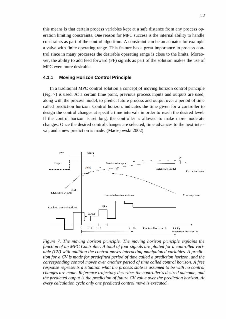
In a traditional MPC control solution a concept of moving horizon control principle (Fig. 7) is used. At a certain time point, previous process inputs and outputs are used, along with the process model, to predict future process and output over a period of time called prediction horizon. Control horizon, indicates the time given for a controller to design the control changes at specific time intervals in order to reach the desired level. If the control horizon is set long, the controller is allowed to make more moderate changes. Once the desired control changes are selected, time advances to the next inter-val, and a new prediction is made. (Maciejowski 2002)
Figure 7. The moving horizon principle. The moving horizon principle explains the function of an MPC Controller. A total of four signals are plotted for a controlled vari-able (CV) with addition the control moves interacting manipulated variables. A predic-tion for a CV is made for predefined period of time called a prediction horizon, and the corresponding control moves over another period of time called control horizon. A free response represents a situation what the process state is assumed to be with no control changes are made. Reference trajectory describes the controller’s desired outcome, and the predicted output is the prediction of future CV value over the prediction horizon. At every calculation cycle only one predicted control move is executed.
23
If no control actions are made, the output is called a free response, where the pro-cess reaches a certain steady-state (SS) after a period of time. A common procedure is to generate a second mathematical model, a reference trajectory, which describes a pro-cess’ assumed behavior. In a simple case, the length of the control horizon is one step, i.e. one change made inside the prediction horizon, where the process output is expected to reach set point value. In such case, the set point and the reference trajectory have only one common point inside the prediction horizon. More commonly, the reference trajec-tory is selected so that is has several mutual points with the set point
4.1.2 MPC Control Principle
MPC uses the mathematical expressions of a process model to predict system behav-ior. These predictions are used to optimize the process over a defined time period. The controller operates according to the following algorithm: First, a process model is de-termined by engineers. The models are usually linear first order models, which are de-termined using typical set point analysis (Chap.2.3.2). Based on the step-response test, the interactions between the process input and output variables can be determined. Quite often first principal models (FPM) are also used for identification (Hedengren et al 2007).
When process behavior is predicted according to the MPC control principle, the control signals that produce the predicted behavior are used to determine a desirable outcome for the controlled variables. An optimizer is used to find the desirable solution within a given time interval regarding a set of process constraints.
4.1.3 Process Variables
A process variable is an indication of current status of a certain part of the process. Accurate measurements are the basis for a successful process modeling. There are a few basic variables, such as pressure, temperature, level, flow, which affect the behavior of a chemical and physical process, and are therefore monitored. Process variables are either direct measurements or derived from the preceding variables. Interaction between two variables can be determined by using analysis methods such as the set point analysis.
As mentioned, process monitoring is equally important to both automation special-ists and the customer. Keeping track on process variables and performance is critical in analyzing and predicting the possible effects and deviations of the particular process. The challenge of process monitoring is to recognize the Key Performance Indices (KPI’s) and further, display them understandably. For multivariate processes, finding KPI’s is especially critical, because of the several dependencies between the variables.
4.1.4 MPC Process Variables
The model predictive controller uses a combination of feedback and feed forward signals generated by models and current plant measurements to calculate future moves in the independent variables that will result in operation that honors all independent and
24
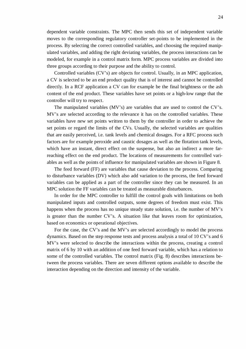
dependent variable constraints. The MPC then sends this set of independent variable moves to the corresponding regulatory controller set-points to be implemented in the process. By selecting the correct controlled variables, and choosing the required manip-ulated variables, and adding the right deviating variables, the process interactions can be modeled, for example in a control matrix form. MPC process variables are divided into three groups according to their purpose and the ability to control.
Controlled variables (CV’s) are objects for control. Usually, in an MPC application, a CV is selected to be an end product quality that is of interest and cannot be controlled directly. In a RCF application a CV can for example be the final brightness or the ash content of the end product. These variables have set points or a high-low range that the controller will try to respect.
The manipulated variables (MV’s) are variables that are used to control the CV’s. MV’s are selected according to the relevance it has on the controlled variables. These variables have new set points written to them by the controller in order to achieve the set points or regard the limits of the CVs. Usually, the selected variables are qualities that are easily perceived, i.e. tank levels and chemical dosages. For a RFC process such factors are for example peroxide and caustic dosages as well as the flotation tank levels, which have an instant, direct effect on the suspense, but also an indirect a more far-reaching effect on the end product. The locations of measurements for controlled vari-ables as well as the points of influence for manipulated variables are shown in Figure 8.
The feed forward (FF) are variables that cause deviation to the process. Comparing to disturbance variables (DV) which also add variation to the process, the feed forward variables can be applied as a part of the controller since they can be measured. In an MPC solution the FF variables can be treated as measurable disturbances.
In order for the MPC controller to fulfill the control goals with limitations on both manipulated inputs and controlled outputs, some degrees of freedom must exist. This happens when the process has no unique steady state solution, i.e. the number of MV’s is greater than the number CV’s. A situation like that leaves room for optimization, based on economics or operational objectives. For the case, the CV’s and the MV’s are selected accordingly to model the process dynamics. Based on the step response tests and process analysis a total of 10 CV’s and 6 MV’s were selected to describe the interactions within the process, creating a control matrix of 6 by 10 with an addition of one feed forward variable, which has a relation to some of the controlled variables. The control matrix (Fig. 8) describes interactions be-tween the process variables. There are seven different options available to describe the interaction depending on the direction and intensity of the variable.
25
Figure 8. MPC control matrix. The matrix shows all the process variables (CV’s, MV’s, and FF’s) as well as their interactions. The intensity of the relationship is determined based on the relative process model gain between a certain CV to MV combination. The effect of the feed forward variable on the controlled variables is also displayed to im-prove the interpretation of the process. The gains are made comparable by fitting them to a normal MV operation range.
Control Matrices describe the relationship between the variables. For a simple 2 in-put 2 output system (two CV’s and two MV’s) the dynamic matrix is
= (4.1)
Where and are the projected Controlled Variables, are step response coef-
ficients, which usually are continuous transfer functions, and and are manipu-lated variable control moves. The objective is to contribute the process by reversing the process dynamics with a right kind of controller. In optimal situation the predicted out-put matches the targeted output. This kind of control strategy applies for a traditional multi input multi output (MIMO) system. Model predictive control strategy includes weighting coefficients, which are used to prioritize certain process parameters according to the control strategy.
26
4.1.5 Feed Forward Variable’s Effect
The feed forward variable, which in this case is the feed forward effective residual ink content (FF ERIC) affects significantly to some of the process controlled variables. During a normal operation the FF ERIC varies significantly depending on state of the process as well as the quality of the feed stock.
4.1.6 Process Constraints
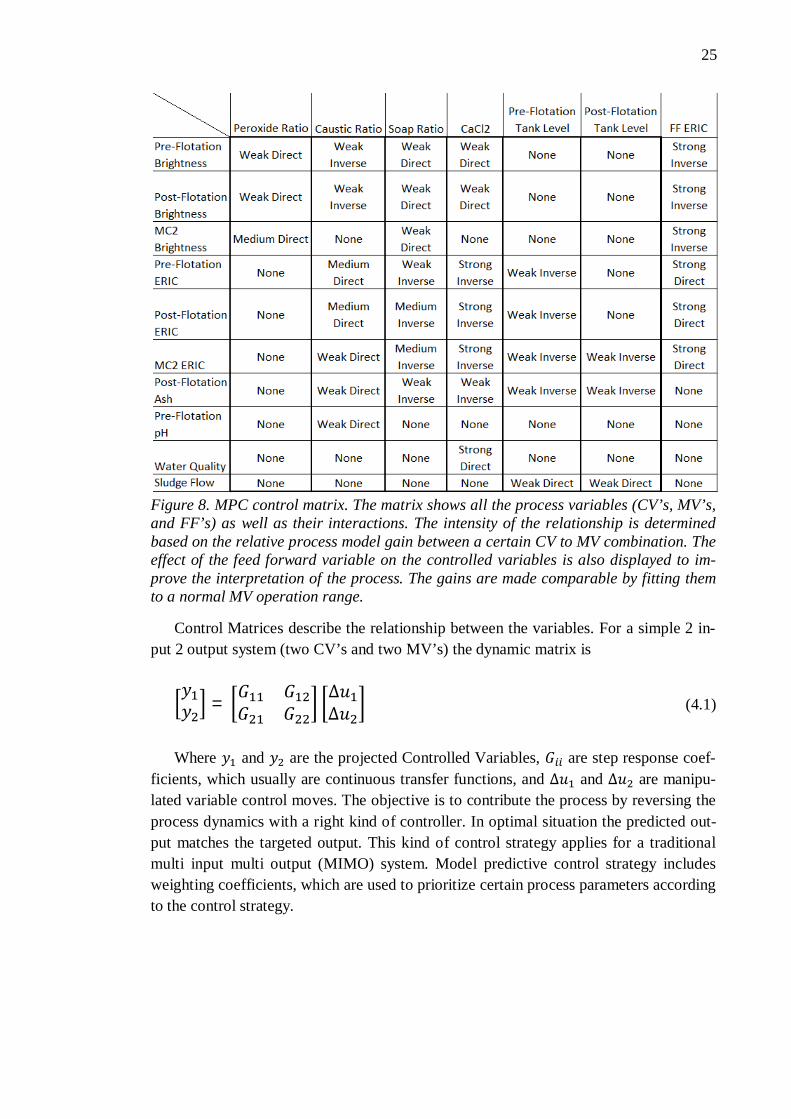
Process constraints (Fig. 9) have a significant role in model predictive control. There are two types of constraint: process state and control signal restrains. An example of a process state constraint is the level of energy in heating process which is wanted to re-duce due to environmental issues, but on the other, to keep it high enough in order to meet the requirements. For traditional PID-controllers, a certain set point is issued to attain a new process state. MPC-controllers are usually given certain low and high limit values for both the MV’s and CV’s, where the controller is allowed to operate.
Figure 9. Process constraints. A multivariate process operation is usually limited by a set of constraints, which can be either physical or predefined quality based limitations. The process constrains are included to the MPC controller as parameters, allowing degrees of freedom to the controller.
A controller with integrating characteristics (PID) combined with a limited actua-tor’s control signal (e.g. valve opening), might end up in situation where error increases significantly. If the controller tries to increase the control signal beyond the actuator capabilities the actual control signal remains the same since it is saturated. A phenome-non where control signal is saturated and the controller tries to increase output is some-times also referred to as windup.
27
Windup complicates the use of controller and can even cause instability to the pro-cess. To prevent wind-up, the operating range of control elements should be limited to the range of the devices they are driving. In PID solutions wind-up is compensated by using anti-wind-up mechanisms (Visioli 2003). However, MPC considers the process constraints, and therefore eliminates the wind-up. The optimum process operating point is usually close to constraint, so the use of MPC is preferred, in order to achieve the best possible result.
4.1.7 Optimizer
In a situation where there are less equations modeling the process behavior than process variables, there are more than one control solutions. In this case, an approximate solution is required. There is more than one method to determine the optimum control. A common method is to use either a Linear Programming (LP) or, the Quadratic Pro-gramming (QP) techniques.
A linear optimization model, which is also known linear programming (LP), is a method to achieve the best outcome in a mathematical model that involves the optimiza-tion of a linear function subject to linear constrains on the variables (Griva et al 2009). Depending on whether the variables are costs or profits, the objective for a linear opti-mization is to either minimize or maximize the function. Eq. 3.2 is an example of a maximized linear programming model
= (4.2)
Where ’s are the particular process variables, and ’s are the corresponding weight coefficients. For a variable that is considered to be profit, the coefficient is positive, and for a variable that is a cost, the coefficient is negative.
In the Quadratic programming method, the optimizing parameters are selected so that, the squared value of the difference between the step-wise target and realized val-ues, minimizes. For MPC, this means the squared difference of reference trajectory and predicted process output values
[ ( + | ) ( + | )] (4.3)
Where P represents the set of common points between the reference trajectory and the set point inside the prediction horizon, r(k) is the reference trajectory values, and y(k) the predicted output values.
4.1.8 Cost function
A cost function is a solution for optimization using programming method. The cost function is defined for all possible output and inputs vectors. For MPC application these
28
vectors represent the CV’s and the MV’s. The form of a cost function can be linear, quadratic, or even exponential, depending on the observed process variables. The target of a cost function is to maximize or minimize the function. A maximized function is sometimes also referred to as a profit function.
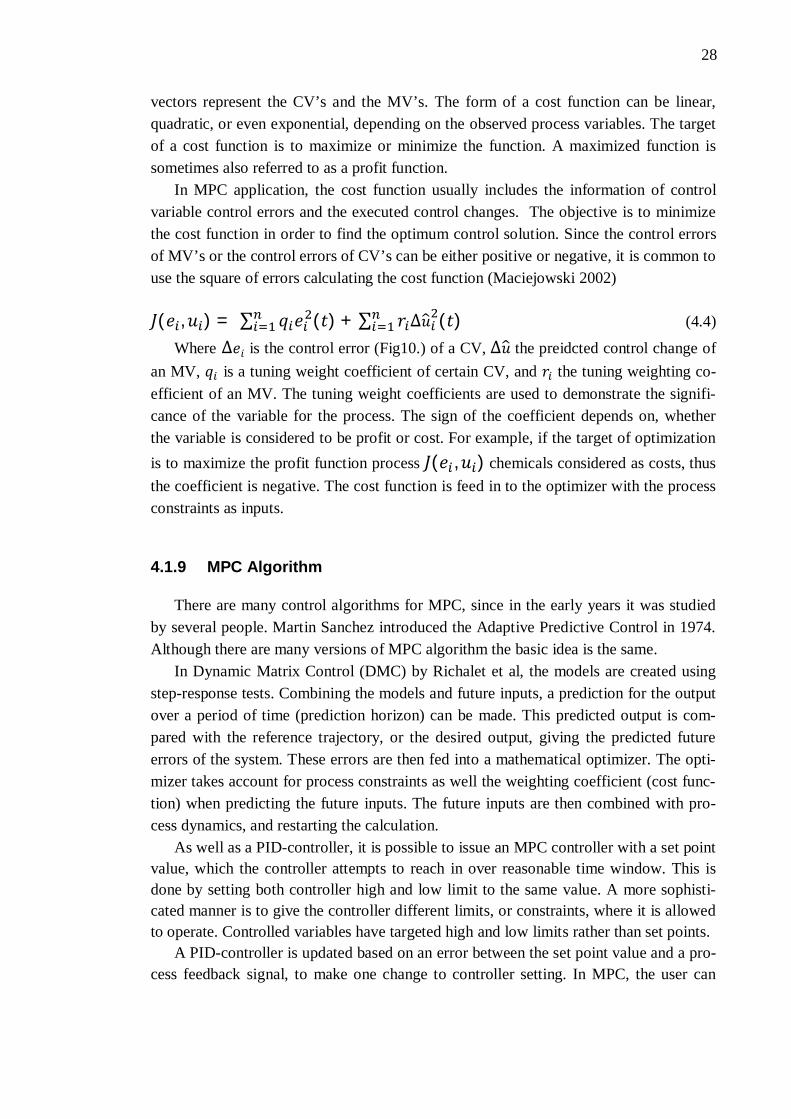
In MPC application, the cost function usually includes the information of control variable control errors and the executed control changes. The objective is to minimize the cost function in order to find the optimum control solution. Since the control errors of MV’s or the control errors of CV’s can be either positive or negative, it is common to use the square of errors calculating the cost function (Maciejowski 2002)
( , ) = ( ) + ( ) (4.4)
Where is the control error (Fig10.) of a CV, the preidcted control change of an MV, is a tuning weight coefficient of certain CV, and the tuning weighting co-efficient of an MV. The tuning weight coefficients are used to demonstrate the signifi-cance of the variable for the process. The sign of the coefficient depends on, whether the variable is considered to be profit or cost. For example, if the target of optimization is to maximize the profit function process ( , ) chemicals considered as costs, thus the coefficient is negative. The cost function is feed in to the optimizer with the process constraints as inputs.
4.1.9 MPC Algorithm
There are many control algorithms for MPC, since in the early years it was studied by several people. Martin Sanchez introduced the Adaptive Predictive Control in 1974. Although there are many versions of MPC algorithm the basic idea is the same.
In Dynamic Matrix Control (DMC) by Richalet et al, the models are created using step-response tests. Combining the models and future inputs, a prediction for the output over a period of time (prediction horizon) can be made. This predicted output is com-pared with the reference trajectory, or the desired output, giving the predicted future errors of the system. These errors are then fed into a mathematical optimizer. The opti-mizer takes account for process constraints as well the weighting coefficient (cost func-tion) when predicting the future inputs. The future inputs are then combined with pro-cess dynamics, and restarting the calculation.
As well as a PID-controller, it is possible to issue an MPC controller with a set point value, which the controller attempts to reach in over reasonable time window. This is done by setting both controller high and low limit to the same value. A more sophisti-cated manner is to give the controller different limits, or constraints, where it is allowed to operate. Controlled variables have targeted high and low limits rather than set points.
A PID-controller is updated based on an error between the set point value and a pro-cess feedback signal, to make one change to controller setting. In MPC, the user can
29
determine the number of future moves the controller will predict. The prediction is up-dated at specified time intervals.
Tuning weights are used to set the importance of violating the low and high limit re-spectively, so that a most critical controlled variable limit violation is prioritized by the controller. Similarly, the manipulated variables have a tuning parameter for defining control move suppression, meaning that the controller can make certain level of control changes according to the affect on the process.
4.2 Performance Solutions RCF Process Control
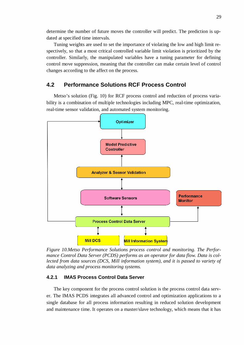
Metso’s solution (Fig. 10) for RCF process control and reduction of process varia-bility is a combination of multiple technologies including MPC, real-time optimization, real-time sensor validation, and automated system monitoring.
Figure 10.Metso Performance Solutions process control and monitoring. The Perfor-mance Control Data Server (PCDS) performs as an operator for data flow. Data is col-lected from data sources (DCS, Mill information system), and it is passed to variety of data analyzing and process monitoring systems.
4.2.1 IMAS Process Control Data Server
The key component for the process control solution is the process control data serv-er. The IMAS PCDS integrates all advanced control and optimization applications to a single database for all process information resulting in reduced solution development and maintenance time. It operates on a master/slave technology, which means that it has
30
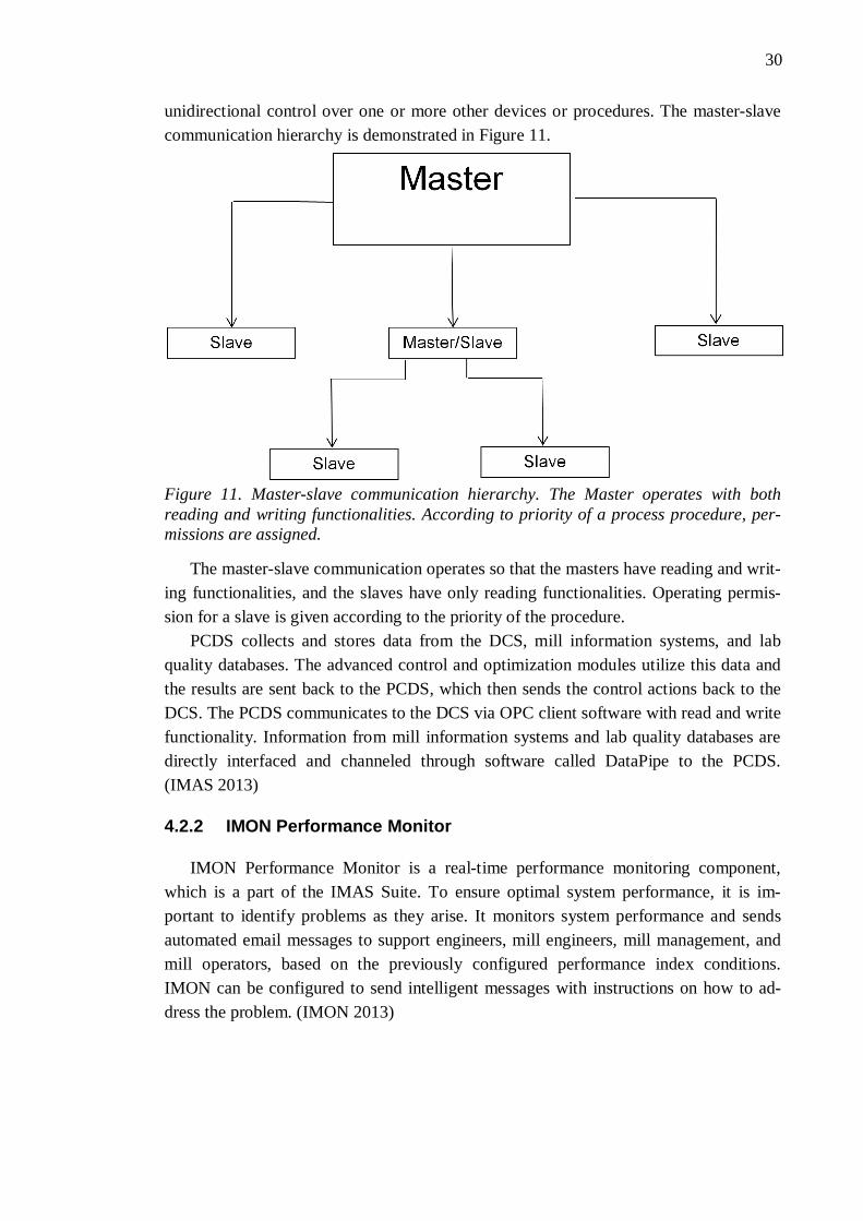
unidirectional control over one or more other devices or procedures. The master-slave communication hierarchy is demonstrated in Figure 11.
Figure 11. Master-slave communication hierarchy. The Master operates with both reading and writing functionalities. According to priority of a process procedure, per-missions are assigned.
The master-slave communication operates so that the masters have reading and writ-ing functionalities, and the slaves have only reading functionalities. Operating permis-sion for a slave is given according to the priority of the procedure.
PCDS collects and stores data from the DCS, mill information systems, and lab quality databases. The advanced control and optimization modules utilize this data and the results are sent back to the PCDS, which then sends the control actions back to the DCS. The PCDS communicates to the DCS via OPC client software with read and write functionality. Information from mill information systems and lab quality databases are directly interfaced and channeled through software called DataPipe to the PCDS. (IMAS 2013)
4.2.2 IMON Performance Monitor
IMON Performance Monitor is a real-time performance monitoring component, which is a part of the IMAS Suite. To ensure optimal system performance, it is im-portant to identify problems as they arise. It monitors system performance and sends automated email messages to support engineers, mill engineers, mill management, and mill operators, based on the previously configured performance index conditions. IMON can be configured to send intelligent messages with instructions on how to ad-dress the problem. (IMON 2013)
31
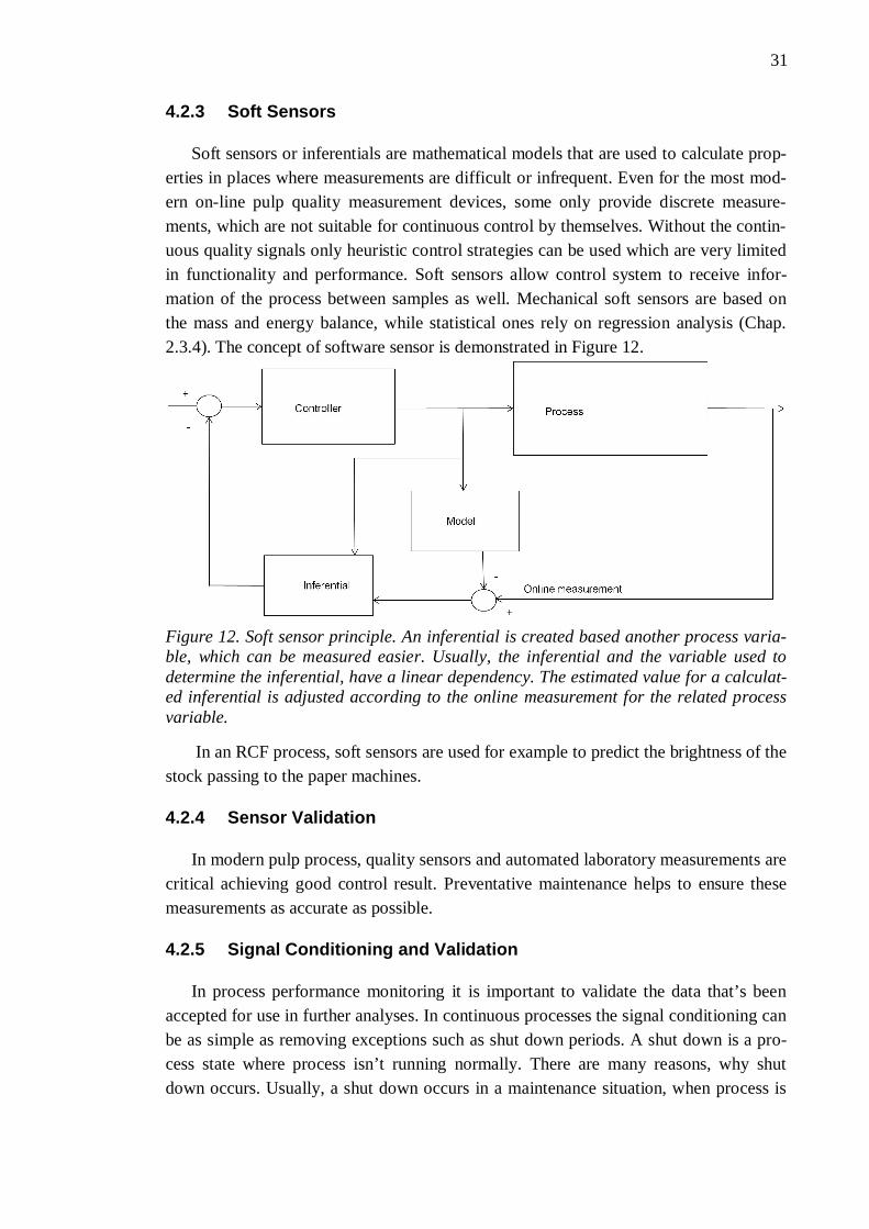
4.2.3 Soft Sensors
Soft sensors or inferentials are mathematical models that are used to calculate prop-erties in places where measurements are difficult or infrequent. Even for the most mod-ern on-line pulp quality measurement devices, some only provide discrete measure-ments, which are not suitable for continuous control by themselves. Without the contin-uous quality signals only heuristic control strategies can be used which are very limited in functionality and performance. Soft sensors allow control system to receive infor-mation of the process between samples as well. Mechanical soft sensors are based on the mass and energy balance, while statistical ones rely on regression analysis (Chap. 2.3.4). The concept of software sensor is demonstrated in Figure 12.
Figure 12. Soft sensor principle. An inferential is created based another process varia-ble, which can be measured easier. Usually, the inferential and the variable used to determine the inferential, have a linear dependency. The estimated value for a calculat-ed inferential is adjusted according to the online measurement for the related process variable.
In an RCF process, soft sensors are used for example to predict the brightness of the stock passing to the paper machines.
4.2.4 Sensor Validation
In modern pulp process, quality sensors and automated laboratory measurements are critical achieving good control result. Preventative maintenance helps to ensure these measurements as accurate as possible.
4.2.5 Signal Conditioning and Validation
In process performance monitoring it is important to validate the data that’s been accepted for use in further analyses. In continuous processes the signal conditioning can be as simple as removing exceptions such as shut down periods. A shut down is a pro-cess state where process isn’t running normally. There are many reasons, why shut down occurs. Usually, a shut down occurs in a maintenance situation, when process is

32
being fixed or updated. More often, shut down is caused by a grade change situation, when the characteristics of the final product are altered.
Production level is usually a good indication for detecting abnormal situation. In Figure 13, production status is represented using a binary signal.
Figure 13. Data filtering and validation. For a successful data analysis, the specific process data need to be validated according to set of conditions. The conditions are usually based on other variables related signals that can also be used to locate the source of an exception.
When the status changed from one to zero, the production rate is abnormal, usually too small. This affects to other process variables as well. These observations are usually left out of process performance analysis, because they are inconsistent, and may lead to incorrect conclusion, thus jeopardizing optimal process performance.
Figure 14 shows the same two signals. However, the “green” process variable signal is missing some of the observations due to data validation.
Figure 14. Validated process data. A quality based process control is usually evaluated by the decrease of normal operation variation. Data validation can mean a decrease of tens of percentages in variation, thus evidencing the importance of defining the right set of data.
33
4.2.6 Calculated Process Data
Some of the data can easily be analyzed directly from the measured signal. Mathe-matical functions provide a good indicator for the process state, and help spotting pro-cess interactions invisible to human eye. Usually, the functions are simple statistical models, like mean or standard deviation values. They are quite informative calculations, but the downside is that to be accurate, the data set must be normally distributed. In many case, the processes are assumed to be normally distributed for simplicity.
4.3 RCF Process Monitoring and Control
RCF is a highly complex process to control with multiple process stages and varia-ble interactions. In order to get real time information about the status of the process, an online process monitoring system is required. In the RCF case, the objects for process monitoring are usually the controlled and manipulated variables, the status of the con-troller, and the process condition. Monitoring can be as simple as displaying the data in a numerical table form, a chart, a diagram or a graphic point or line trend.
Process performance monitoring and control requires effective solutions for data measuring and collection, visualization, and analyzing. Data must be filtered and vali-dated accordingly for the controller, to avoid undesirable outcomes.
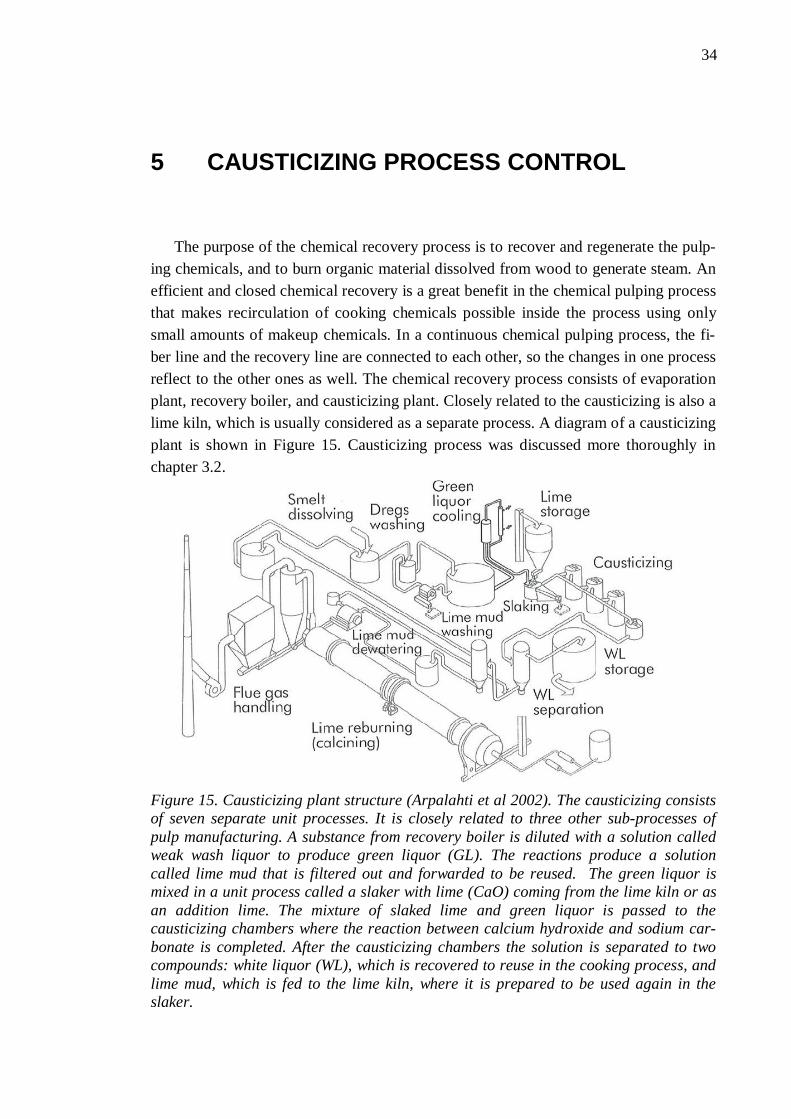
34
5 CAUSTICIZING PROCESS CONTROL
The purpose of the chemical recovery process is to recover and regenerate the pulp-ing chemicals, and to burn organic material dissolved from wood to generate steam. An efficient and closed chemical recovery is a great benefit in the chemical pulping process that makes recirculation of cooking chemicals possible inside the process using only small amounts of makeup chemicals. In a continuous chemical pulping process, the fi-ber line and the recovery line are connected to each other, so the changes in one process reflect to the other ones as well. The chemical recovery process consists of evaporation plant, recovery boiler, and causticizing plant. Closely related to the causticizing is also a lime kiln, which is usually considered as a separate process. A diagram of a causticizing plant is shown in Figure 15. Causticizing process was discussed more thoroughly in chapter 3.2.
Figure 15. Causticizing plant structure (Arpalahti et al 2002). The causticizing consists of seven separate unit processes. It is closely related to three other sub-processes of pulp manufacturing. A substance from recovery boiler is diluted with a solution called weak wash liquor to produce green liquor (GL). The reactions produce a solution called lime mud that is filtered out and forwarded to be reused. The green liquor is mixed in a unit process called a slaker with lime (CaO) coming from the lime kiln or as an addition lime. The mixture of slaked lime and green liquor is passed to the causticizing chambers where the reaction between calcium hydroxide and sodium car-bonate is completed. After the causticizing chambers the solution is separated to two compounds: white liquor (WL), which is recovered to reuse in the cooking process, and lime mud, which is fed to the lime kiln, where it is prepared to be used again in the slaker.

35
5.1.1 Process Variables
In causticizing process, a large variation of process qualities is highly undesirable, thus an active process monitoring is essential. The process variables are selected accord-ingly to model the process dynamics. Based on the step response tests and process analysis the monitored variables were selected to fulfil the objective of causticizing which is to produce consistent alkali for cooking process. The monitored variables are listed in Table 1. Table 1. Causticizing process variables
Process Variable Unit 1. Causticizing chamber causticizing efficiency
CE-%
Last Causticizing chamber causticizing efficiency
CE-%
White liquor causticizing efficiency CE-% Green liquor to slaker flow l/s Green liquor temperature °C Slaker temperature °C Slaker temperature difference °C Dissolver Green liquor TTA g/l Green liquor to slaker TTA g/l Dissolver density kg/m3 Green liquor density kg/m3 The quality of the end product depends highly on the composition of the green liquor; therefore it can be viewed as a feeding variable. The focused control objectives are causticizing efficiency, slaker temperature difference, and slaker TTA-control.
5.2 Model Reference Advanced Causticizing Control
The Model-Reference Adaptive System (MRAS) was originally proposed to solve a problem in which the performance specifications are given in terms of a reference mod-el. The formulation of adaptive control as a stochastic control problem was given by Feldbaum (1965). While initially direct adaptive control schemes have only considered in continuous time, the discrete time direct adaptive schemes and applications were in-troduced later (Landau 1971) and (Bethoux 1973).
Much like for an MPC solution, the reference model in MRAC solution indicates the ideal process output created by the control change. The Model reference control param-eters however, are updated based on the error between reference model and the actual output.
Model reference adaptive controller has two control loops. The inner loop consists of the process and an ordinary feedback controller (Fig. 16). The outer loop adjusts the
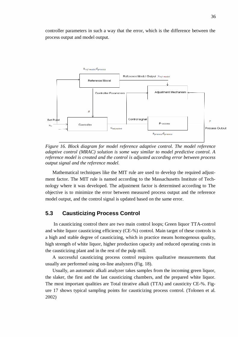
36
controller parameters in such a way that the error, which is the difference between the process output and model output.
Figure 16. Block diagram for model reference adaptive control. The model reference adaptive control (MRAC) solution is some way similar to model predictive control. A reference model is created and the control is adjusted according error between process output signal and the reference model.
Mathematical techniques like the MIT rule are used to develop the required adjust-ment factor. The MIT rule is named according to the Massachusetts Institute of Tech-nology where it was developed. The adjustment factor is determined according to The objective is to minimize the error between measured process output and the reference model output, and the control signal is updated based on the same error.
5.3 Causticizing Process Control
In causticizing control there are two main control loops; Green liquor TTA-control and white liquor causticizing efficiency (CE-%) control. Main target of these controls is a high and stable degree of causticizing, which in practice means homogenous quality, high strength of white liquor, higher production capacity and reduced operating costs in the causticizing plant and in the rest of the pulp mill.
A successful causticizing process control requires qualitative measurements that usually are performed using on-line analyzers (Fig. 18).
Usually, an automatic alkali analyzer takes samples from the incoming green liquor, the slaker, the first and the last causticizing chambers, and the prepared white liquor. The most important qualities are Total titrative alkali (TTA) and causticity CE-%. Fig-ure 17 shows typical sampling points for causticizing process control. (Tolonen et al. 2002)
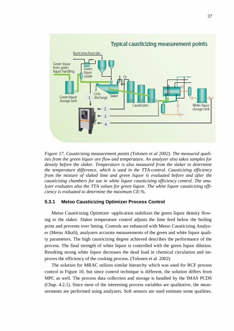
37
Figure 17. Causticizing measurement points (Tolonen et al 2002). The measured quali-ties from the green liquor are flow and temperature. An analyzer also takes samples for density before the slaker. Temperature is also measured from the slaker to determine the temperature difference, which is used in the TTA-control. Causticizing efficiency from the mixture of slaked lime and green liquor is evaluated before and after the causticizing chambers for use in white liquor causticizing efficiency control. The ana-lyzer evaluates also the TTA values for green liquor. The white liquor causticizing effi-ciency is evaluated to determine the maximum CE-%.
5.3.1 Metso Causticizing Optimizer Process Control
Metso Causticizing Optimizer -application stabilizes the green liquor density flow-ing to the slaker. Slaker temperature control adjusts the lime feed below the boiling point and prevents over liming. Controls are enhanced with Metso Causticizing Analyz-er (Metso Alkali), analyzers accurate measurements of the green and white liquor quali-ty parameters. The high causticizing degree achieved describes the performance of the process. The final strength of white liquor is controlled with the green liquor dilution. Resulting strong white liquor decreases the dead load in chemical circulation and im-proves the efficiency of the cooking process. (Tolonen et al. 2002)
The solution for MRAC utilizes similar hierarchy which was used for RCF process control in Figure 10, but since control technique is different, the solution differs from MPC as well. The process data collection and storage is handled by the IMAS PCDS (Chap. 4.2.1). Since most of the interesting process variables are qualitative, the meas-urements are performed using analyzers. Soft sensors are used estimate some qualities.
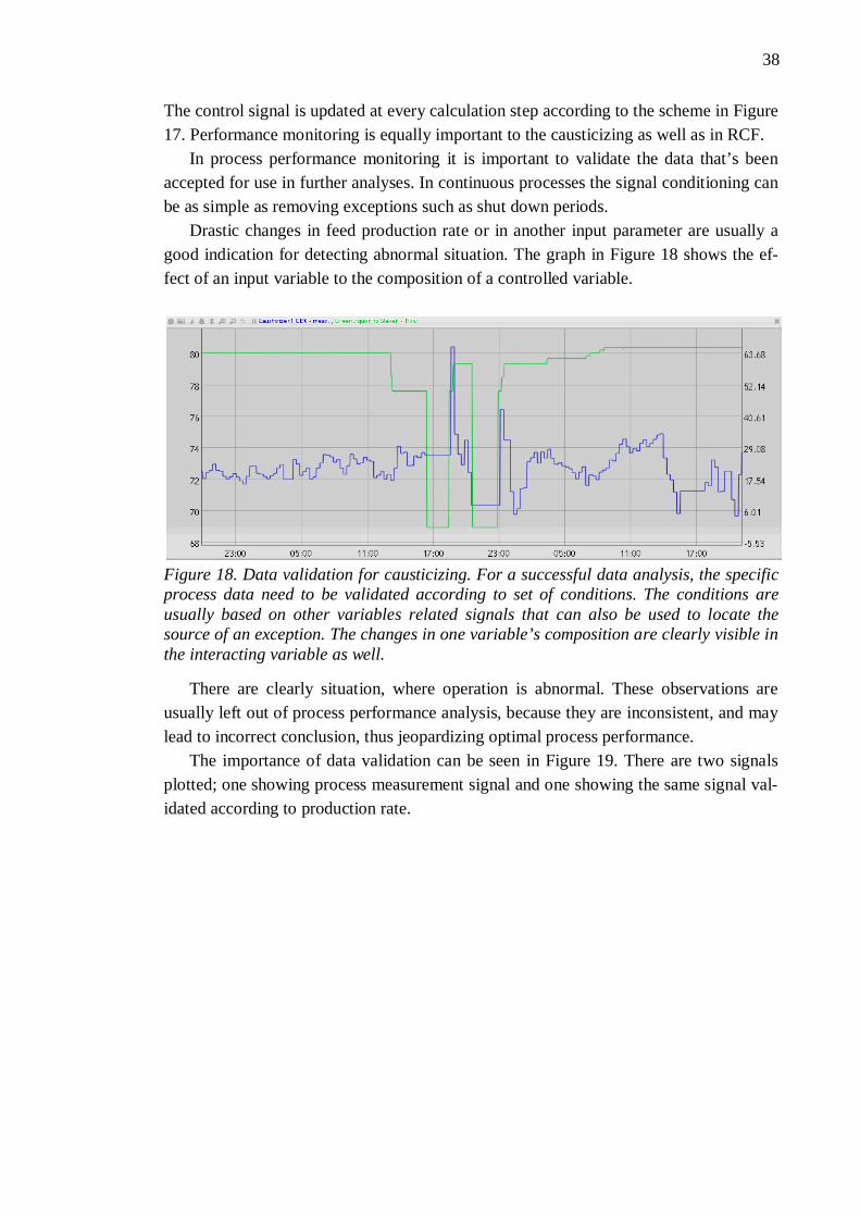
38
The control signal is updated at every calculation step according to the scheme in Figure 17. Performance monitoring is equally important to the causticizing as well as in RCF.
In process performance monitoring it is important to validate the data that’s been accepted for use in further analyses. In continuous processes the signal conditioning can be as simple as removing exceptions such as shut down periods.
Drastic changes in feed production rate or in another input parameter are usually a good indication for detecting abnormal situation. The graph in Figure 18 shows the ef-fect of an input variable to the composition of a controlled variable.
Figure 18. Data validation for causticizing. For a successful data analysis, the specific process data need to be validated according to set of conditions. The conditions are usually based on other variables related signals that can also be used to locate the source of an exception. The changes in one variable’s composition are clearly visible in the interacting variable as well.
There are clearly situation, where operation is abnormal. These observations are usually left out of process performance analysis, because they are inconsistent, and may lead to incorrect conclusion, thus jeopardizing optimal process performance.
The importance of data validation can be seen in Figure 19. There are two signals plotted; one showing process measurement signal and one showing the same signal val-idated according to production rate.
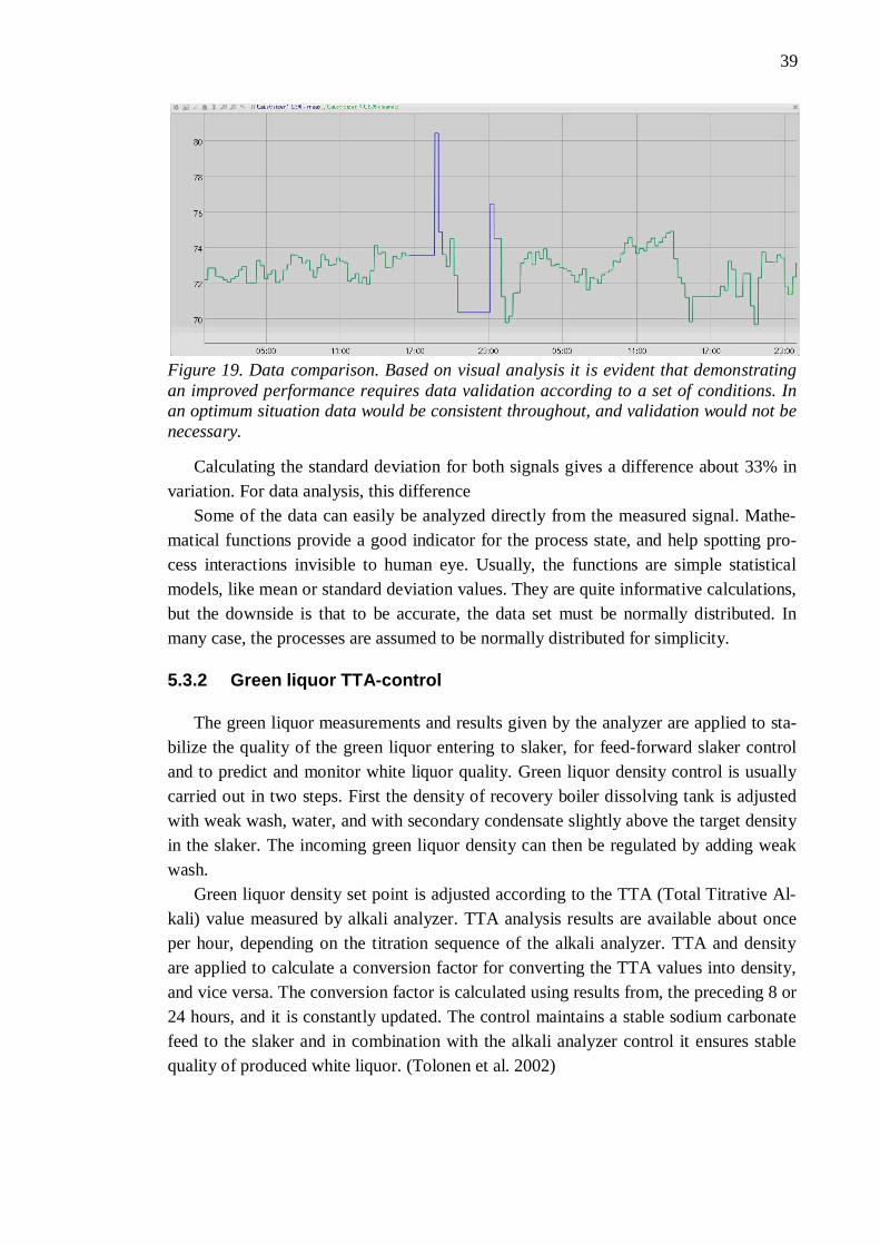
39
Figure 19. Data comparison. Based on visual analysis it is evident that demonstrating an improved performance requires data validation according to a set of conditions. In an optimum situation data would be consistent throughout, and validation would not be necessary.
Calculating the standard deviation for both signals gives a difference about 33% in variation. For data analysis, this difference
Some of the data can easily be analyzed directly from the measured signal. Mathe-matical functions provide a good indicator for the process state, and help spotting pro-cess interactions invisible to human eye. Usually, the functions are simple statistical models, like mean or standard deviation values. They are quite informative calculations, but the downside is that to be accurate, the data set must be normally distributed. In many case, the processes are assumed to be normally distributed for simplicity.
5.3.2 Green liquor TTA-control
The green liquor measurements and results given by the analyzer are applied to sta-bilize the quality of the green liquor entering to slaker, for feed-forward slaker control and to predict and monitor white liquor quality. Green liquor density control is usually carried out in two steps. First the density of recovery boiler dissolving tank is adjusted with weak wash, water, and with secondary condensate slightly above the target density in the slaker. The incoming green liquor density can then be regulated by adding weak wash.
Green liquor density set point is adjusted according to the TTA (Total Titrative Al-kali) value measured by alkali analyzer. TTA analysis results are available about once per hour, depending on the titration sequence of the alkali analyzer. TTA and density are applied to calculate a conversion factor for converting the TTA values into density, and vice versa. The conversion factor is calculated using results from, the preceding 8 or 24 hours, and it is constantly updated. The control maintains a stable sodium carbonate feed to the slaker and in combination with the alkali analyzer control it ensures stable quality of produced white liquor. (Tolonen et al. 2002)

40
5.3.3 CE%- control
The CE-% control is based on feed forward calculations for lime feed to green liq-uor flow ratio, green liquor to slaker temperature difference control, and for maximum theoretical CE-%. Based on the calculations, a model for the white liquor (WL) quality control is created.
The temperature difference between slaker and green liquor indicates the relative progress of the causticizing reaction. Short-term changes in temperature difference indi-cate changes in either quantity or quality of raw materials entering the slaker. The green liquor flow consistency is the single biggest cause for quality variations. In the long run the temperature difference control alone is not able to maintain the target causticizing result, as changes in lime quality and the temperature level have a significant effect on scaling and causticizing kinetics. For this reason, the absolute measurement results of the composition of green liquor, lime milk, and white liquor are extremely valuable for slaker controls.
Causticizing process is an example of continuous process with multiple internal and external process interactions. The complexity of the process and significant process de-lays require a modern control solution. The selected case was concluded at an ongoing site, so the required step response tests were already conducted, and the process models are in place. The required measurements are performed using the mill’s existing analyz-ers and measuring devices, which are stored in the Process control data server (PCDS) and mill’s information system (MIS). The conditioned is stored in another database. Both untreated and computational data are used to implement the performance monitor-ing tool for model reference adaptive control.
Predicting the outcome of a time series can be improved by adding a weighted func-tion as a filter (Chap. 2.3.5). A simple moving average considers all the values of a data set equally, thus including invalid observations as well. This of course weakens the pre-diction. By adding a weighted coefficient, the calculation takes more significantly ac-count for, usually, the previous values.
As well as in the MPC performance monitoring case, the used signals need be vali-dated, so that exceptions, like shut down periods are ruled out.
5.4 Causticizing Process Control and Monitoring
Causticizing process is one of the most critical parts of the chemical pulp plant, since it is one connection points between the fiber line and the recovery line. For a high-ly interactive process much like the RCF, it is desirable to have monitoring system, which allows real time online evaluation. Process wise, the most interesting part in causticizing is the quality end product, white liquor, which is the chemical used in cook-ing process. For a control engineer’s point of view, the topic of interest is to detect how well the implemented controller model responses to the process changes.

41
Comparing to traditional fixed gain PID-controllers, the adaptive controllers are very effective to handle the situations where process parameter and environmental vari-ations are evident. The controller parameters are adjusted accordingly with the aim of minimizing the error between parameter output and the desired reference model. Adjust-ing can be done using several techniques like the MIT rule.
Process performance monitoring and control requires effective solutions for data measuring and collection, visualization, and analyzing. Data must be filtered and vali-dated accordingly for the controller, to reach maximum process performance.
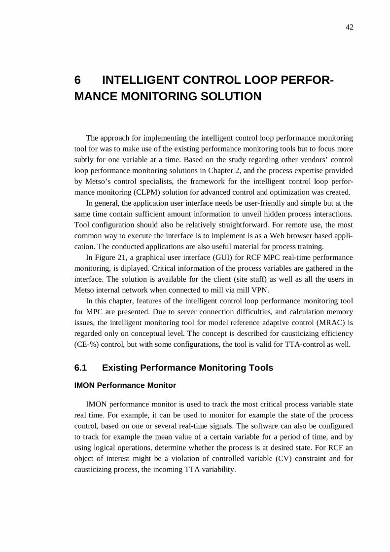
42
6 INTELLIGENT CONTROL LOOP PERFOR-MANCE MONITORING SOLUTION
The approach for implementing the intelligent control loop performance monitoring tool for was to make use of the existing performance monitoring tools but to focus more subtly for one variable at a time. Based on the study regarding other vendors’ control loop performance monitoring solutions in Chapter 2, and the process expertise provided by Metso’s control specialists, the framework for the intelligent control loop perfor-mance monitoring (CLPM) solution for advanced control and optimization was created.
In general, the application user interface needs be user-friendly and simple but at the same time contain sufficient amount information to unveil hidden process interactions. Tool configuration should also be relatively straightforward. For remote use, the most common way to execute the interface is to implement is as a Web browser based appli-cation. The conducted applications are also useful material for process training.
In Figure 21, a graphical user interface (GUI) for RCF MPC real-time performance monitoring, is diplayed. Critical information of the process variables are gathered in the interface. The solution is available for the client (site staff) as well as all the users in Metso internal network when connected to mill via mill VPN.
In this chapter, features of the intelligent control loop performance monitoring tool for MPC are presented. Due to server connection difficulties, and calculation memory issues, the intelligent monitoring tool for model reference adaptive control (MRAC) is regarded only on conceptual level. The concept is described for causticizing efficiency (CE-%) control, but with some configurations, the tool is valid for TTA-control as well.
6.1 Existing Performance Monitoring Tools
IMON Performance Monitor
IMON performance monitor is used to track the most critical process variable state real time. For example, it can be used to monitor for example the state of the process control, based on one or several real-time signals. The software can also be configured to track for example the mean value of a certain variable for a period of time, and by using logical operations, determine whether the process is at desired state. For RCF an object of interest might be a violation of controlled variable (CV) constraint and for causticizing process, the incoming TTA variability.
43
Performance Report
Automated Excel-reports based on event-driven Microsoft Visual Basic program-ming language are sent daily, weekly or monthly. IMAS Excel Add-in toolbar allows collecting IMAS data to Excel. The reports include both tabular and graphical data of the process variables. Unlike IMON, the performance reports give information about the process past and are therefore more suitable for offline data analysis.
WebMon
WebMon is a web-based monitoring tool, which allows remote access to process monitoring for both customers and process engineers. WebMon includes graphical pro-cess history data similarly to the performance reports, but has also real-time user inter-face for online process review.
6.2 Intelligent Control Loop Performance Monitoring Tool for MPC
The intelligent control loop performance monitoring tool (Fig. 21) is configured us-ing a combination php, html, and python coding. All the basic mathematical calcula-tions are executed using the functions of python included numerical Python (NumPy) library (Lutz, 2009). The signal conditioning is done using different functions provided by Matplotlib (Hunter, 2007) extension for NumPy. The used data is stored in a process control data server (PCDS), where it is updated based on the data provided by the dis-tributed control system or mill information system. As demonstrated in Figure 11, the process control data server acts as a master for the system, meaning that it handles the activity of other sources by giving permissions for certain acts according to the priority of the procedure.
6.2.1 Controlled Variable Performance Monitoring
Performance monitoring for controlled variables includes both online process meas-urement data, and calculated data based on the process signals. The signals are selected to cover the model of a certain variable, to understand control actions, and to help engi-neers to make adjustments for the process models. The tabular values are real-time pro-cess signals from the PCDS. The graphic display includes history data for a time period of two days as a default setting. For history data evaluation, the time window can be adjusted accordingly.
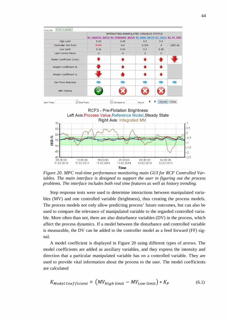
44
Figure 20. MPC real-time performance monitoring main GUI for RCF Controlled Var-iables. The main interface is designed to support the user in figuring out the process problems. The interface includes both real time features as well as history trending.
Step response tests were used to determine interactions between manipulated varia-bles (MV) and one controlled variable (brightness), thus creating the process models. The process models not only allow predicting process’ future outcomes, but can also be used to compare the relevance of manipulated variable to the regarded controlled varia-ble. More often than not, there are also disturbance variables (DV) in the process, which affect the process dynamics. If a model between the disturbance and controlled variable is measurable, the DV can be added to the controller model as a feed forward (FF) sig-nal.
A model coefficient is displayed in Figure 20 using different types of arrows. The model coefficients are added as auxiliary variables, and they express the intensity and direction that a particular manipulated variable has on a controlled variable. They are used to provide vital information about the process to the user. The model coefficients are calculated
= (6.1)
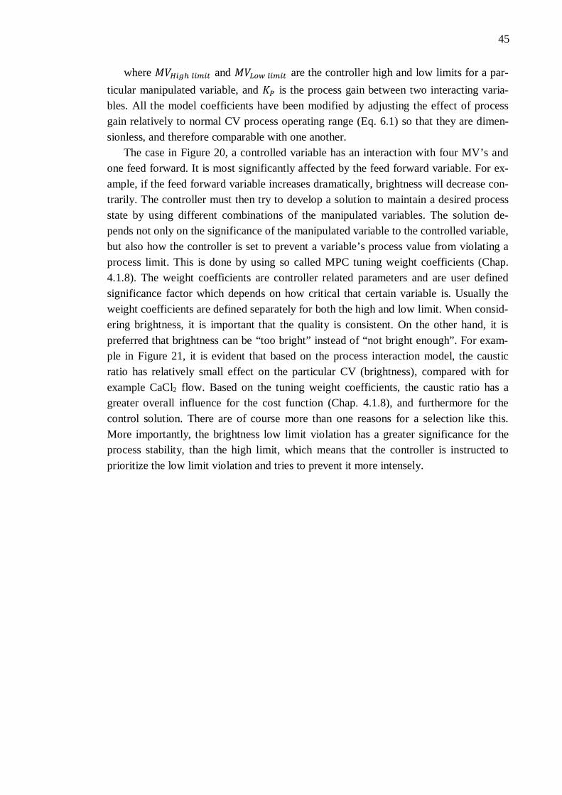
45
where and are the controller high and low limits for a par-ticular manipulated variable, and is the process gain between two interacting varia-bles. All the model coefficients have been modified by adjusting the effect of process gain relatively to normal CV process operating range (Eq. 6.1) so that they are dimen-sionless, and therefore comparable with one another.
The case in Figure 20, a controlled variable has an interaction with four MV’s and one feed forward. It is most significantly affected by the feed forward variable. For ex-ample, if the feed forward variable increases dramatically, brightness will decrease con-trarily. The controller must then try to develop a solution to maintain a desired process state by using different combinations of the manipulated variables. The solution de-pends not only on the significance of the manipulated variable to the controlled variable, but also how the controller is set to prevent a variable’s process value from violating a process limit. This is done by using so called MPC tuning weight coefficients (Chap. 4.1.8). The weight coefficients are controller related parameters and are user defined significance factor which depends on how critical that certain variable is. Usually the weight coefficients are defined separately for both the high and low limit. When consid-ering brightness, it is important that the quality is consistent. On the other hand, it is preferred that brightness can be “too bright” instead of “not bright enough”. For exam-ple in Figure 21, it is evident that based on the process interaction model, the caustic ratio has relatively small effect on the particular CV (brightness), compared with for example CaCl2 flow. Based on the tuning weight coefficients, the caustic ratio has a greater overall influence for the cost function (Chap. 4.1.8), and furthermore for the control solution. There are of course more than one reasons for a selection like this. More importantly, the brightness low limit violation has a greater significance for the process stability, than the high limit, which means that the controller is instructed to prioritize the low limit violation and tries to prevent it more intensely.

46
Figure 21. Controlled variable (CV) tabular section. The table shows momentary set point values for interacting MV’s, as well as the possible feed forward variable. A mod-el coefficient arrow describes the direction and intensity which an MV has over the CV. The weight coefficients are presented using arrows as well. The direction is equal to the MV to CV interaction as the model coefficient. The arrow size tells the controller the significance of a particular CV limit violation for the process. Set point direction is used to enlighten the controller’s decision making in an MV limit violation situation.
In an MV limit violation situation, the set point direction indicates where controller is forcing the MV set point based on the difference of the last two observation points. However, it is more common that the MV set point value is saturated at a high or low limit. A limit violation for MV usually occurs only in an exception, such as shut down periods.
The data that is used to calculate the set point direction is separated from the actual measured signal from the process using two kinds of filters. First, the calculation is only valid, when the line is in a normal production state. Secondly, a more specified condi-tion checks whether the signal violates either user defined controller high or low limit. If one or more conditions are invalid, the data is being filtered out. Figure 22 shows the filtered signal based on the two conditions.
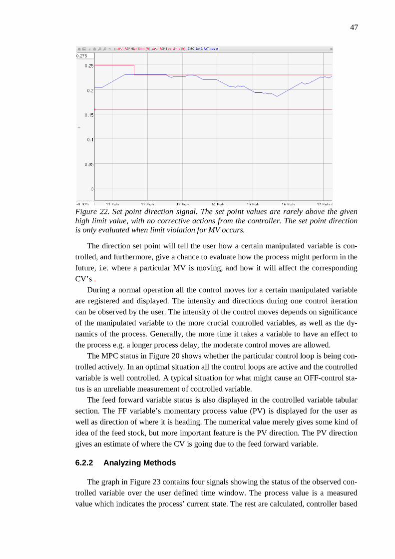
47
Figure 22. Set point direction signal. The set point values are rarely above the given high limit value, with no corrective actions from the controller. The set point direction is only evaluated when limit violation for MV occurs.
The direction set point will tell the user how a certain manipulated variable is con-trolled, and furthermore, give a chance to evaluate how the process might perform in the future, i.e. where a particular MV is moving, and how it will affect the corresponding CV’s .
During a normal operation all the control moves for a certain manipulated variable are registered and displayed. The intensity and directions during one control iteration can be observed by the user. The intensity of the control moves depends on significance of the manipulated variable to the more crucial controlled variables, as well as the dy-namics of the process. Generally, the more time it takes a variable to have an effect to the process e.g. a longer process delay, the moderate control moves are allowed.
The MPC status in Figure 20 shows whether the particular control loop is being con-trolled actively. In an optimal situation all the control loops are active and the controlled variable is well controlled. A typical situation for what might cause an OFF-control sta-tus is an unreliable measurement of controlled variable.
The feed forward variable status is also displayed in the controlled variable tabular section. The FF variable’s momentary process value (PV) is displayed for the user as well as direction of where it is heading. The numerical value merely gives some kind of idea of the feed stock, but more important feature is the PV direction. The PV direction gives an estimate of where the CV is going due to the feed forward variable.
6.2.2 Analyzing Methods
The graph in Figure 23 contains four signals showing the status of the observed con-trolled variable over the user defined time window. The process value is a measured value which indicates the process’ current state. The rest are calculated, controller based
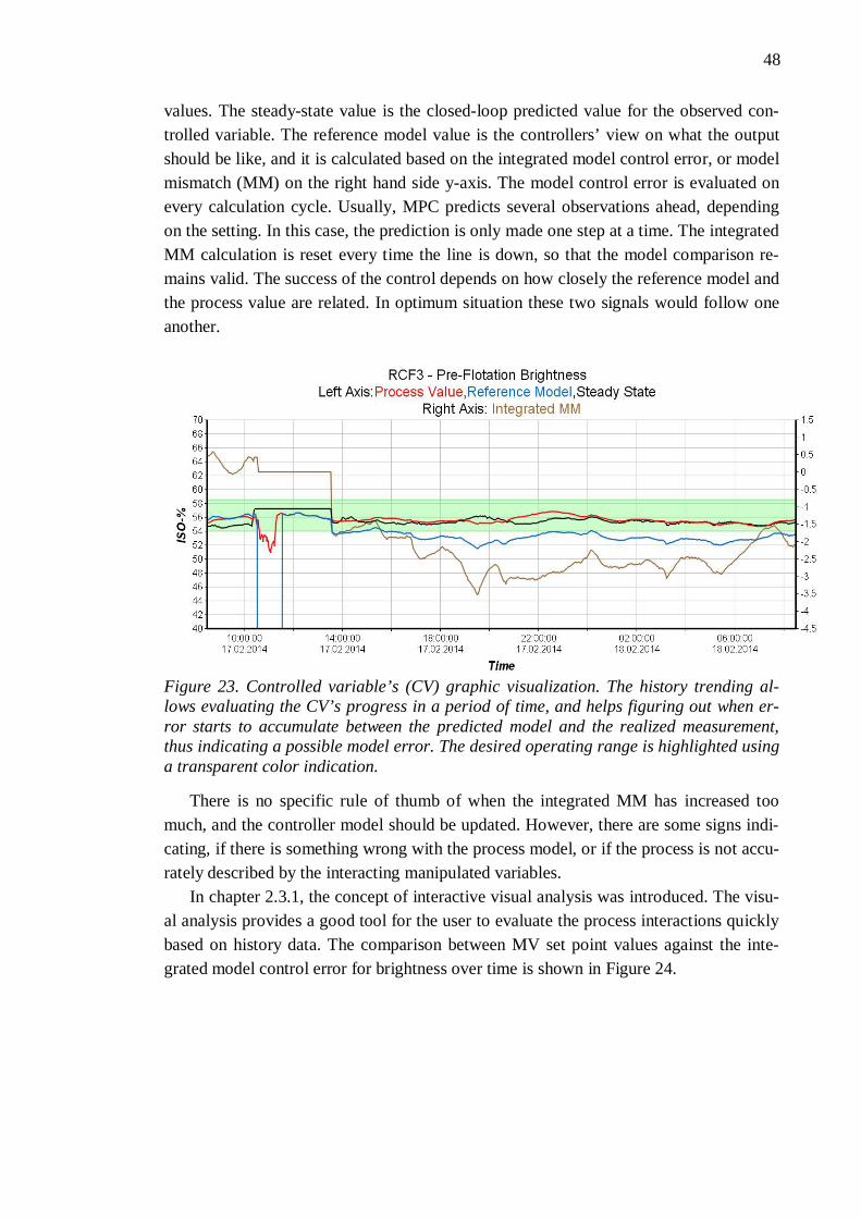
48
values. The steady-state value is the closed-loop predicted value for the observed con-trolled variable. The reference model value is the controllers’ view on what the output should be like, and it is calculated based on the integrated model control error, or model mismatch (MM) on the right hand side y-axis. The model control error is evaluated on every calculation cycle. Usually, MPC predicts several observations ahead, depending on the setting. In this case, the prediction is only made one step at a time. The integrated MM calculation is reset every time the line is down, so that the model comparison re-mains valid. The success of the control depends on how closely the reference model and the process value are related. In optimum situation these two signals would follow one another.
Figure 23. Controlled variable’s (CV) graphic visualization. The history trending al-lows evaluating the CV’s progress in a period of time, and helps figuring out when er-ror starts to accumulate between the predicted model and the realized measurement, thus indicating a possible model error. The desired operating range is highlighted using a transparent color indication.
There is no specific rule of thumb of when the integrated MM has increased too much, and the controller model should be updated. However, there are some signs indi-cating, if there is something wrong with the process model, or if the process is not accu-rately described by the interacting manipulated variables.
In chapter 2.3.1, the concept of interactive visual analysis was introduced. The visu-al analysis provides a good tool for the user to evaluate the process interactions quickly based on history data. The comparison between MV set point values against the inte-grated model control error for brightness over time is shown in Figure 24.
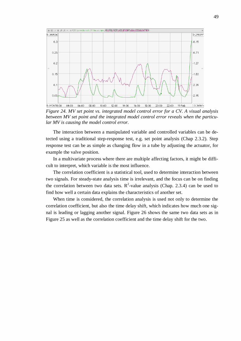
49
Figure 24. MV set point vs. integrated model control error for a CV. A visual analysis between MV set point and the integrated model control error reveals when the particu-lar MV is causing the model control error.
The interaction between a manipulated variable and controlled variables can be de-tected using a traditional step-response test, e.g. set point analysis (Chap 2.3.2). Step response test can be as simple as changing flow in a tube by adjusting the actuator, for example the valve position.
In a multivariate process where there are multiple affecting factors, it might be diffi-cult to interpret, which variable is the most influence.
The correlation coefficient is a statistical tool, used to determine interaction between two signals. For steady-state analysis time is irrelevant, and the focus can be on finding the correlation between two data sets. R2-value analysis (Chap. 2.3.4) can be used to find how well a certain data explains the characteristics of another set.
When time is considered, the correlation analysis is used not only to determine the correlation coefficient, but also the time delay shift, which indicates how much one sig-nal is leading or lagging another signal. Figure 26 shows the same two data sets as in Figure 25 as well as the correlation coefficient and the time delay shift for the two.

50
Figure 25. Correlation coefficient and time delay shift. A correlation analysis gives a statistical point of view of the relationship between the interacting variables. The lower graph shows correlation and the calculated correlation time delay in hours.
The correlation coefficient and the time delay shift are evaluated inside a three hour time window. The time delay shift is calculated using the maximum value (Chap. 2.3.5) of a cross-correlation signal. The time delay shift is determined by selecting the maxi-mum correlation value inside the time window, and evaluating the corresponding value, i.e. at what time point the correlation is the strongest. In Figure 25, it is presumed that the controlled variable is lagging, since the manipulated variable is what the controller is changing. The time delay shift value can then be used to determine how much unex-plained lag there is between the compared signals, i.e., how the model needs to be changed, in order to a response at desired time point. If similar time delay shift occurs repeatedly, there might be a systematic error in the process model, and it needs to be updated.
Controlled variable performance monitoring tool allows a closer inspection of a cer-tain MV to CV interaction by clicking a reference link for desired manipulated variable in the main interface. The reference link is opened to a new window (Fig 26).
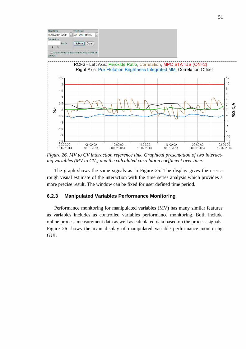
51
Figure 26. MV to CV interaction reference link. Graphical presentation of two interact-ing variables (MV to CV,) and the calculated correlation coefficient over time.
The graph shows the same signals as in Figure 25. The display gives the user a rough visual estimate of the interaction with the time series analysis which provides a more precise result. The window can be fixed for user defined time period.
6.2.3 Manipulated Variables Performance Monitoring
Performance monitoring for manipulated variables (MV) has many similar features as variables includes as controlled variables performance monitoring. Both include online process measurement data as well as calculated data based on the process signals. Figure 26 shows the main display of manipulated variable performance monitoring GUI.
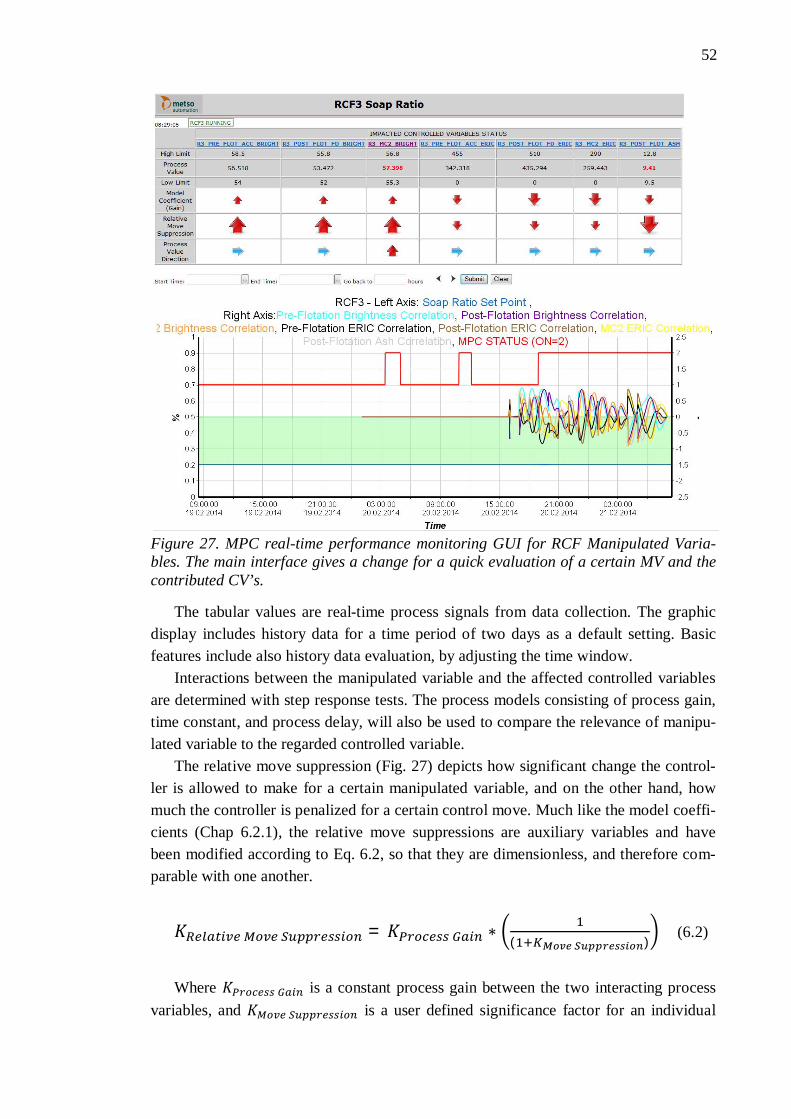
52
Figure 27. MPC real-time performance monitoring GUI for RCF Manipulated Varia-bles. The main interface gives a change for a quick evaluation of a certain MV and the contributed CV’s.
The tabular values are real-time process signals from data collection. The graphic display includes history data for a time period of two days as a default setting. Basic features include also history data evaluation, by adjusting the time window.
Interactions between the manipulated variable and the affected controlled variables are determined with step response tests. The process models consisting of process gain, time constant, and process delay, will also be used to compare the relevance of manipu-lated variable to the regarded controlled variable.
The relative move suppression (Fig. 27) depicts how significant change the control-ler is allowed to make for a certain manipulated variable, and on the other hand, how much the controller is penalized for a certain control move. Much like the model coeffi-cients (Chap 6.2.1), the relative move suppressions are auxiliary variables and have been modified according to Eq. 6.2, so that they are dimensionless, and therefore com-parable with one another.
=( )
(6.2)
Where is a constant process gain between the two interacting process
variables, and is a user defined significance factor for an individual
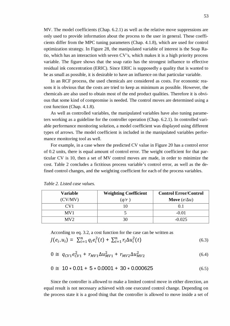
53
MV. The model coefficients (Chap. 6.2.1) as well as the relative move suppressions are only used to provide information about the process to the user in general. These coeffi-cients differ from the MPC tuning parameters (Chap. 4.1.8), which are used for control optimization strategy. In Figure 28, the manipulated variable of interest is the Soap Ra-tio, which has an interaction with seven CV’s, which makes it is a high priority process variable. The figure shows that the soap ratio has the strongest influence to effective residual ink concentration (ERIC). Since ERIC is supposedly a quality that is wanted to be as small as possible, it is desirable to have an influence on that particular variable.
In an RCF process, the used chemicals are considered as costs. For economic rea-sons it is obvious that the costs are tried to keep as minimum as possible. However, the chemicals are also used to obtain most of the end product qualities. Therefore it is obvi-ous that some kind of compromise is needed. The control moves are determined using a cost function (Chap. 4.1.8).
As well as controlled variables, the manipulated variables have also tuning parame-ters working as a guideline for the controller operation (Chap. 6.2.1). In controlled vari-able performance monitoring solution, a model coefficient was displayed using different types of arrows. The model coefficient is included in the manipulated variables perfor-mance monitoring tool as well.
For example, in a case where the predicted CV value in Figure 20 has a control error of 0.2 units, there is equal amount of control error. The weight coefficient for that par-ticular CV is 10, then a set of MV control moves are made, in order to minimize the cost. Table 2 concludes a fictitious process variable’s control error, as well as the de-fined control changes, and the weighting coefficient for each of the process variables.
Table 2. Listed case values.
Variable (CV/MV)
Weighting Coefficient ( / )
Control Error/Control Move ( / )
CV1 10 0.1 MV1 5 -0.01 MV2 30 -0.025
According to eq. 3.2, a cost function for the case can be written as ( , ) = ( ) + ( ) (6.3)
+ + (6.4)
10 0.01 + 5 0.0001 + 30 0.000625 (6.5)
Since the controller is allowed to make a limited control move in either direction, an
equal result is not necessary achieved with one executed control change. Depending on the process state it is a good thing that the controller is allowed to move inside a set of
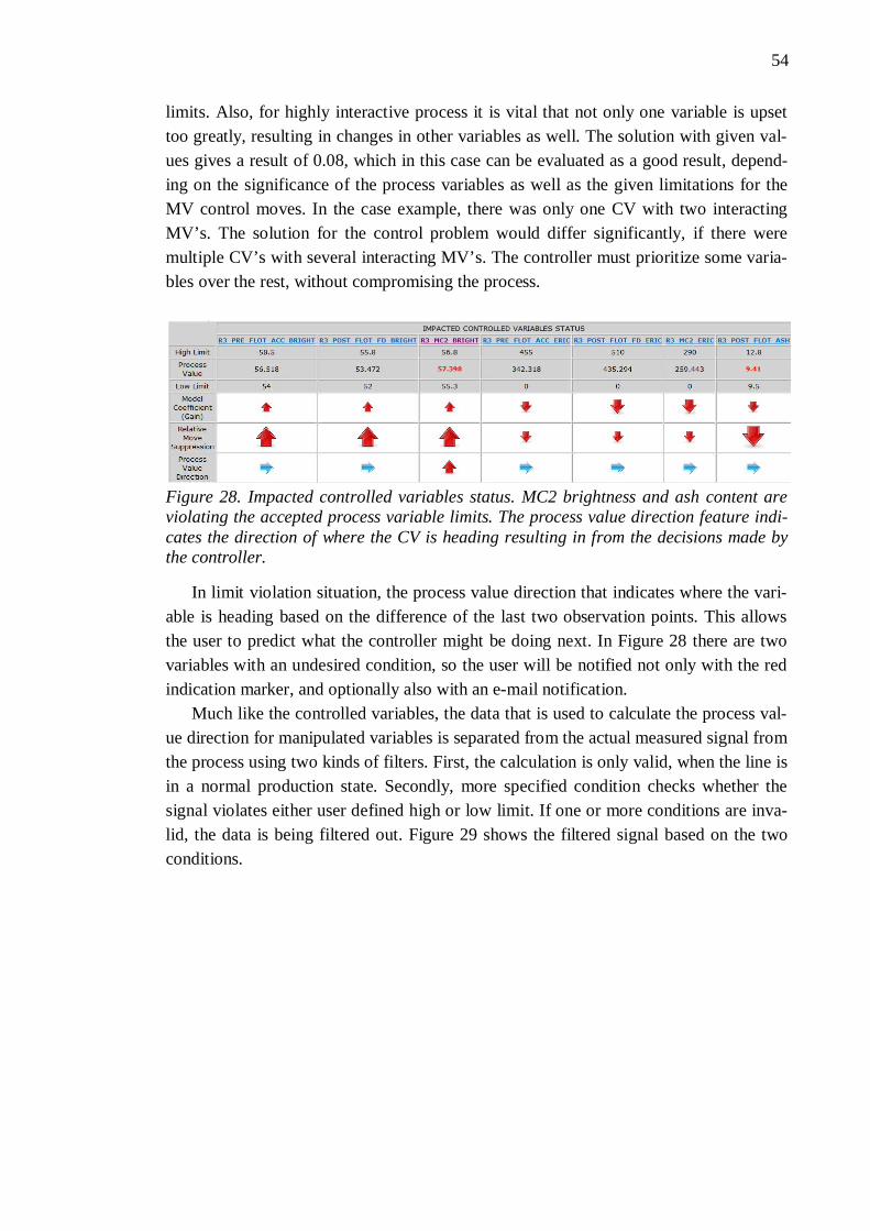
54
limits. Also, for highly interactive process it is vital that not only one variable is upset too greatly, resulting in changes in other variables as well. The solution with given val-ues gives a result of 0.08, which in this case can be evaluated as a good result, depend-ing on the significance of the process variables as well as the given limitations for the MV control moves. In the case example, there was only one CV with two interacting MV’s. The solution for the control problem would differ significantly, if there were multiple CV’s with several interacting MV’s. The controller must prioritize some varia-bles over the rest, without compromising the process.
Figure 28. Impacted controlled variables status. MC2 brightness and ash content are violating the accepted process variable limits. The process value direction feature indi-cates the direction of where the CV is heading resulting in from the decisions made by the controller.
In limit violation situation, the process value direction that indicates where the vari-able is heading based on the difference of the last two observation points. This allows the user to predict what the controller might be doing next. In Figure 28 there are two variables with an undesired condition, so the user will be notified not only with the red indication marker, and optionally also with an e-mail notification.
Much like the controlled variables, the data that is used to calculate the process val-ue direction for manipulated variables is separated from the actual measured signal from the process using two kinds of filters. First, the calculation is only valid, when the line is in a normal production state. Secondly, more specified condition checks whether the signal violates either user defined high or low limit. If one or more conditions are inva-lid, the data is being filtered out. Figure 29 shows the filtered signal based on the two conditions.
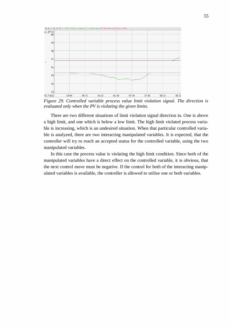
55
Figure 29. Controlled variable process value limit violation signal. The direction is evaluated only when the PV is violating the given limits.
There are two different situations of limit violation signal direction in. One is above a high limit, and one which is below a low limit. The high limit violated process varia-ble is increasing, which is an undesired situation. When that particular controlled varia-ble is analyzed, there are two interacting manipulated variables. It is expected, that the controller will try to reach an accepted status for the controlled variable, using the two manipulated variables.
In this case the process value is violating the high limit condition. Since both of the manipulated variables have a direct effect on the controlled variable, it is obvious, that the next control move must be negative. If the control for both of the interacting manip-ulated variables is available, the controller is allowed to utilize one or both variables.
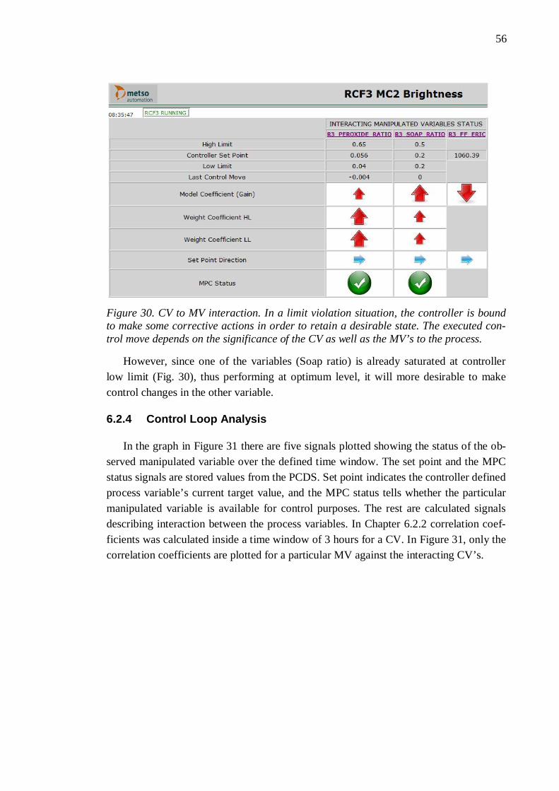
56
Figure 30. CV to MV interaction. In a limit violation situation, the controller is bound to make some corrective actions in order to retain a desirable state. The executed con-trol move depends on the significance of the CV as well as the MV’s to the process.
However, since one of the variables (Soap ratio) is already saturated at controller low limit (Fig. 30), thus performing at optimum level, it will more desirable to make control changes in the other variable.
6.2.4 Control Loop Analysis
In the graph in Figure 31 there are five signals plotted showing the status of the ob-served manipulated variable over the defined time window. The set point and the MPC status signals are stored values from the PCDS. Set point indicates the controller defined process variable’s current target value, and the MPC status tells whether the particular manipulated variable is available for control purposes. The rest are calculated signals describing interaction between the process variables. In Chapter 6.2.2 correlation coef-ficients was calculated inside a time window of 3 hours for a CV. In Figure 31, only the correlation coefficients are plotted for a particular MV against the interacting CV’s.
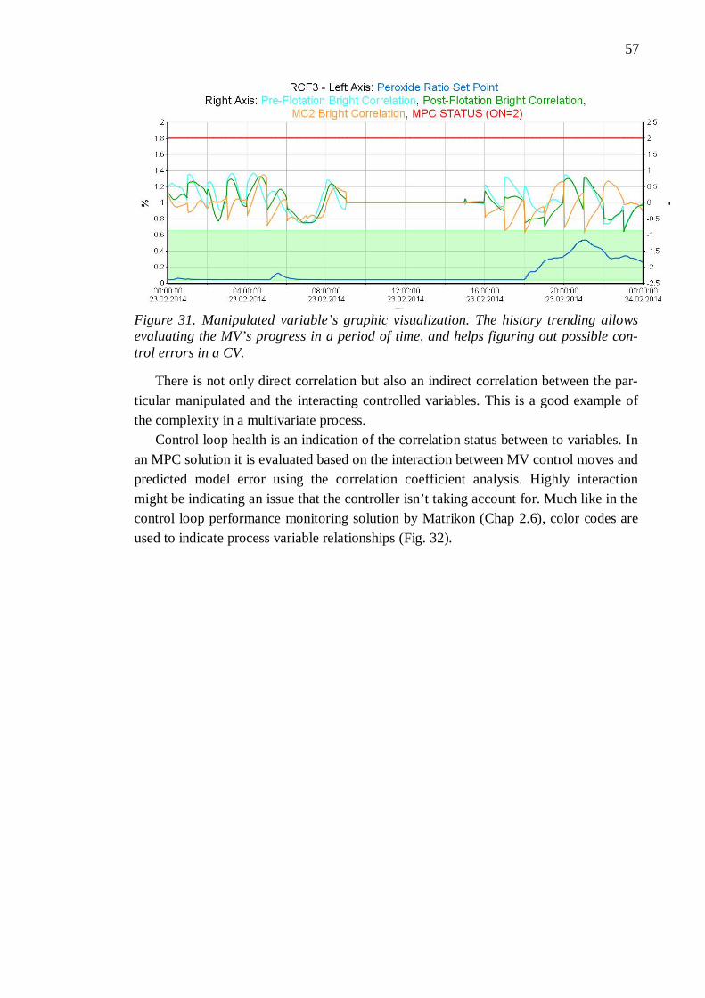
57
Figure 31. Manipulated variable’s graphic visualization. The history trending allows evaluating the MV’s progress in a period of time, and helps figuring out possible con-trol errors in a CV.
There is not only direct correlation but also an indirect correlation between the par-ticular manipulated and the interacting controlled variables. This is a good example of the complexity in a multivariate process.
Control loop health is an indication of the correlation status between to variables. In an MPC solution it is evaluated based on the interaction between MV control moves and predicted model error using the correlation coefficient analysis. Highly interaction might be indicating an issue that the controller isn’t taking account for. Much like in the control loop performance monitoring solution by Matrikon (Chap 2.6), color codes are used to indicate process variable relationships (Fig. 32).

58
Figure 32. Control loop health chart. The control loop health chart shows the relation-ships between all the controlled and the manipulated variables. The purpose color indi-cation is to describe the intensity of the correlation with red color indicating a strong correlation, yellow a medium correlation, and green a weak correlation. Black color indicates no correlation between two variables. A strong correlation might be denoting a model error between two variables.
For both of the multivariate process cases reviewed in chapters 5.3 and 5.4, it is cru-cial to be able to detect variable interactions for high performing control solution. Time series analysis was used to find the most correlated process variables. The analysis is carried out over a section time that is selected accordingly for the particular process. For the MPC tool time window was selected to be 3 hours. For suitable monitoring purpos-es, the data should be reviewed in time sections of 12 hours. The correlation coefficient would be evaluated inside the time window every three hours.
A quantitative measure of the performance of a system, like the performance index, is necessary for the operation of parameter optimization, and design of the control sys-tem. There are different types of performance indices being used, depending on the pur-pose. The integrated average error (IAE) is calculated as the average absolute value of error between process variable (PV) and a set point (SP). Usually it is calculated as an indication of performance over a period of time, and used for computer simulation stud-ies (Dorf & Bishop 2000)
= | | (Eq. 6.6)
Where k is the number of observations used to calculate the integrated average error. The IAE value ranges between 0 and 100%. Obviously, a smaller value means a better result. The IAE value is proportional to the costs of a control loop (Chap. 4.1.8).
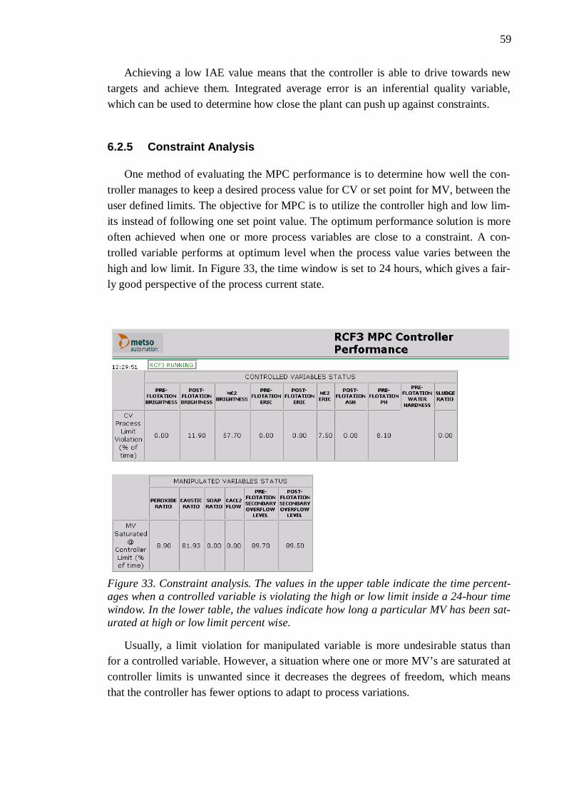
59
Achieving a low IAE value means that the controller is able to drive towards new targets and achieve them. Integrated average error is an inferential quality variable, which can be used to determine how close the plant can push up against constraints.
6.2.5 Constraint Analysis
One method of evaluating the MPC performance is to determine how well the con-troller manages to keep a desired process value for CV or set point for MV, between the user defined limits. The objective for MPC is to utilize the controller high and low lim-its instead of following one set point value. The optimum performance solution is more often achieved when one or more process variables are close to a constraint. A con-trolled variable performs at optimum level when the process value varies between the high and low limit. In Figure 33, the time window is set to 24 hours, which gives a fair-ly good perspective of the process current state.
Figure 33. Constraint analysis. The values in the upper table indicate the time percent-ages when a controlled variable is violating the high or low limit inside a 24-hour time window. In the lower table, the values indicate how long a particular MV has been sat-urated at high or low limit percent wise.
Usually, a limit violation for manipulated variable is more undesirable status than for a controlled variable. However, a situation where one or more MV’s are saturated at controller limits is unwanted since it decreases the degrees of freedom, which means that the controller has fewer options to adapt to process variations.

60
6.2.6 Predicted Control Change
In chapter 6.2.1, a concept set point direction was introduced. The set point direction was used to determine where the controller is forcing the particular manipulated varia-ble to move based on the set point changes.
Figure 34. Controller predictive action. The measured CV process value is violating the defined process limits. The controller has three possible solutions to affect the CV; to use either MV’s, or the two of them. The selection is limited by the significance of an MV control move as well as the current set point of the MV.
In Figure 34, the monitored controlled variable is way below a desired level. Since there are two interacting manipulated variables the controller is expected to make con-trol changes to one or both MV’s. Since both MV’s have a direct influence to the CV, the expected corrective action is to increase the values of one or both MV’s, so the con-troller’s prediction would be to increase both MV’s. The executed control move de-pends on the defined tuning parameters (move suppressions), i.e. how much penalty is generated for the given control move. By closer observation, it appears that one of the MV’s is at high limit, so it would be undesirable to increase the value of that MV. An improvement for the tool is to display not only the controller’s set point direction during a controller limit violation but also the predictive control change, or what kind of changes the controller would like to perform.
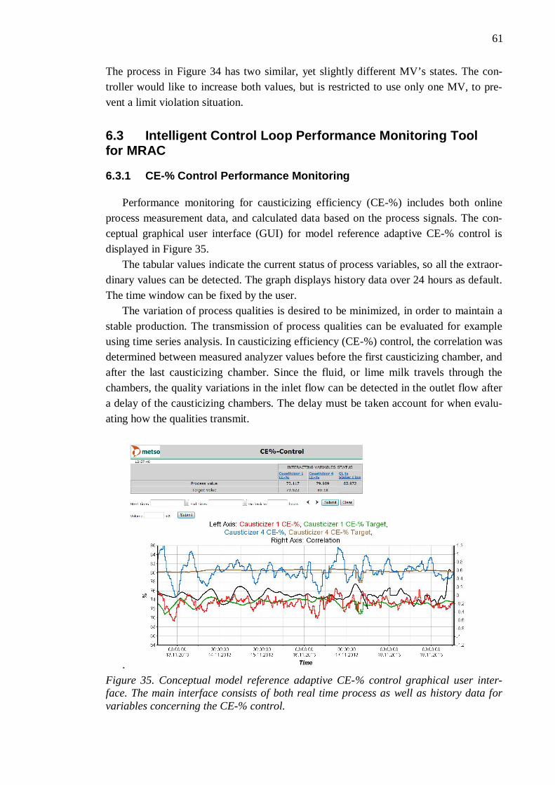
61
The process in Figure 34 has two similar, yet slightly different MV’s states. The con-troller would like to increase both values, but is restricted to use only one MV, to pre-vent a limit violation situation.
6.3 Intelligent Control Loop Performance Monitoring Tool for MRAC
6.3.1 CE-% Control Performance Monitoring
Performance monitoring for causticizing efficiency (CE-%) includes both online process measurement data, and calculated data based on the process signals. The con-ceptual graphical user interface (GUI) for model reference adaptive CE-% control is displayed in Figure 35.
The tabular values indicate the current status of process variables, so all the extraor-dinary values can be detected. The graph displays history data over 24 hours as default. The time window can be fixed by the user.
The variation of process qualities is desired to be minimized, in order to maintain a stable production. The transmission of process qualities can be evaluated for example using time series analysis. In causticizing efficiency (CE-%) control, the correlation was determined between measured analyzer values before the first causticizing chamber, and after the last causticizing chamber. Since the fluid, or lime milk travels through the chambers, the quality variations in the inlet flow can be detected in the outlet flow after a delay of the causticizing chambers. The delay must be taken account for when evalu-ating how the qualities transmit.
. Figure 35. Conceptual model reference adaptive CE-% control graphical user inter-face. The main interface consists of both real time process as well as history data for variables concerning the CE-% control.
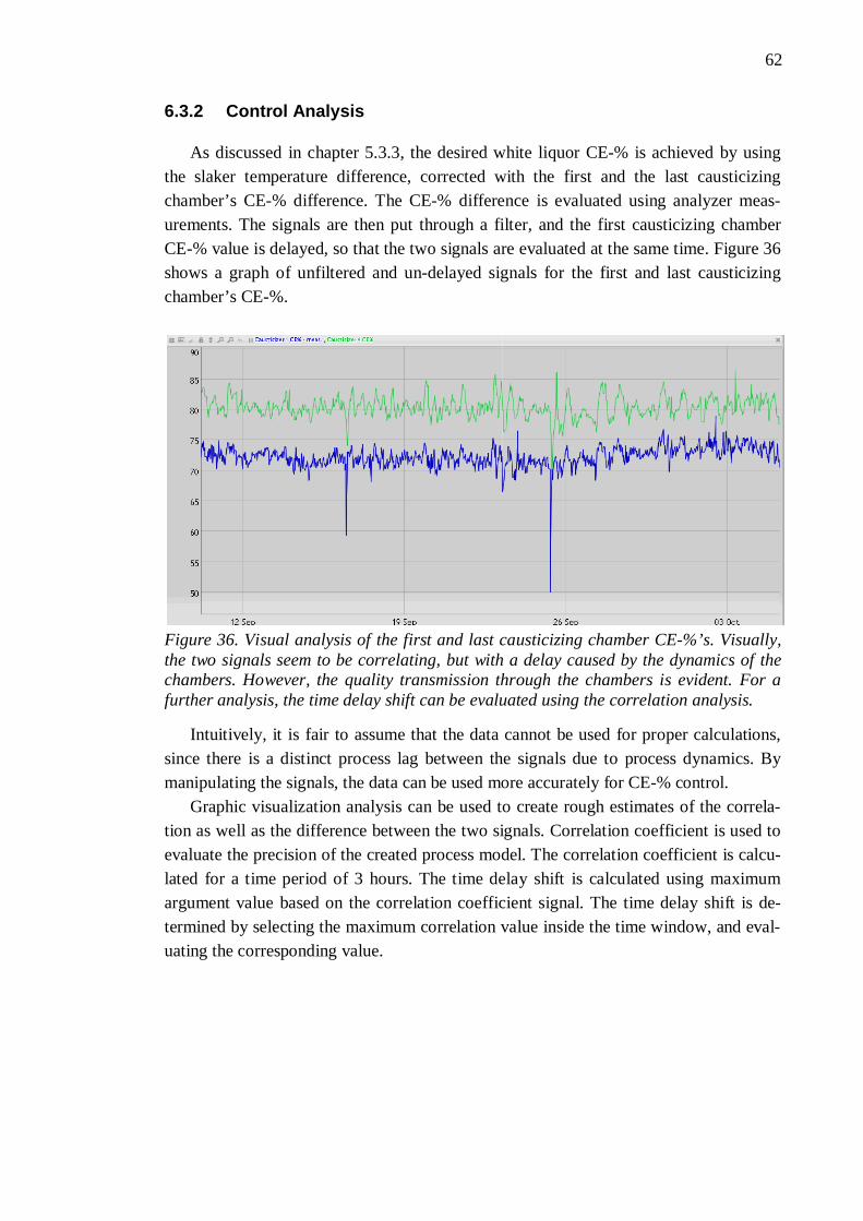
62
6.3.2 Control Analysis
As discussed in chapter 5.3.3, the desired white liquor CE-% is achieved by using the slaker temperature difference, corrected with the first and the last causticizing chamber’s CE-% difference. The CE-% difference is evaluated using analyzer meas-urements. The signals are then put through a filter, and the first causticizing chamber CE-% value is delayed, so that the two signals are evaluated at the same time. Figure 36 shows a graph of unfiltered and un-delayed signals for the first and last causticizing chamber’s CE-%.
Figure 36. Visual analysis of the first and last causticizing chamber CE-%’s. Visually, the two signals seem to be correlating, but with a delay caused by the dynamics of the chambers. However, the quality transmission through the chambers is evident. For a further analysis, the time delay shift can be evaluated using the correlation analysis.
Intuitively, it is fair to assume that the data cannot be used for proper calculations, since there is a distinct process lag between the signals due to process dynamics. By manipulating the signals, the data can be used more accurately for CE-% control.
Graphic visualization analysis can be used to create rough estimates of the correla-tion as well as the difference between the two signals. Correlation coefficient is used to evaluate the precision of the created process model. The correlation coefficient is calcu-lated for a time period of 3 hours. The time delay shift is calculated using maximum argument value based on the correlation coefficient signal. The time delay shift is de-termined by selecting the maximum correlation value inside the time window, and eval-uating the corresponding value.
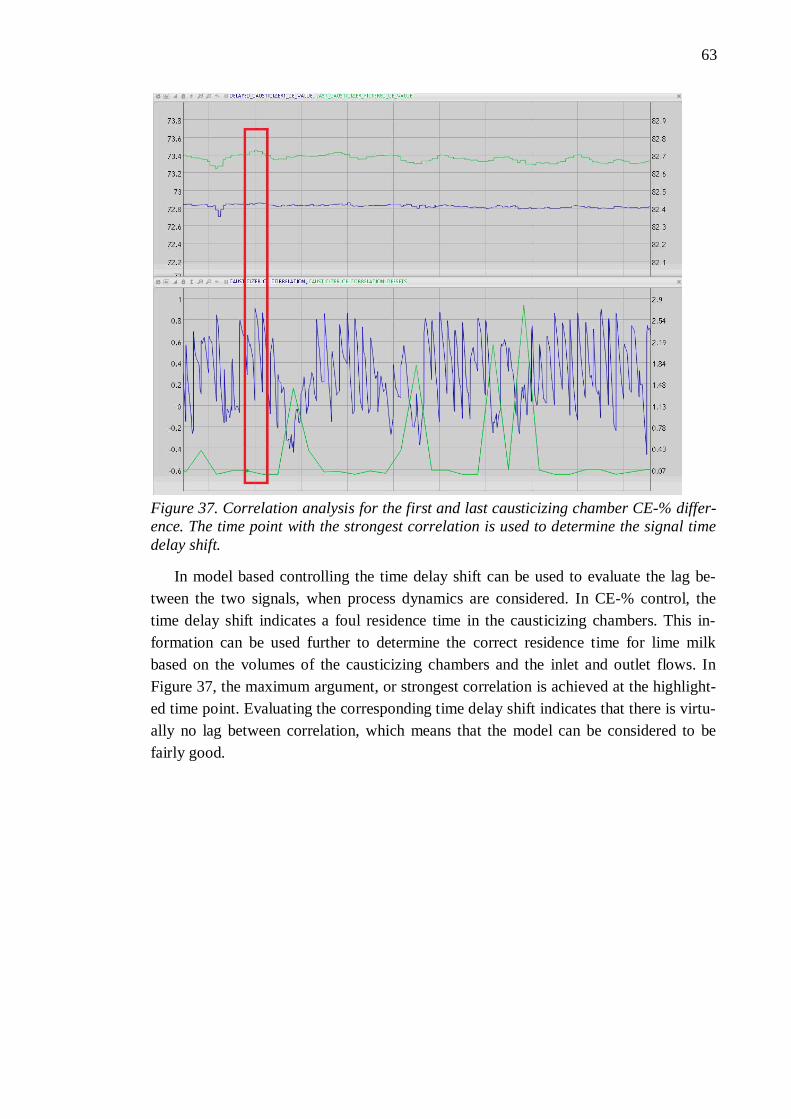
63
Figure 37. Correlation analysis for the first and last causticizing chamber CE-% differ-ence. The time point with the strongest correlation is used to determine the signal time delay shift.
In model based controlling the time delay shift can be used to evaluate the lag be-tween the two signals, when process dynamics are considered. In CE-% control, the time delay shift indicates a foul residence time in the causticizing chambers. This in-formation can be used further to determine the correct residence time for lime milk based on the volumes of the causticizing chambers and the inlet and outlet flows. In Figure 37, the maximum argument, or strongest correlation is achieved at the highlight-ed time point. Evaluating the corresponding time delay shift indicates that there is virtu-ally no lag between correlation, which means that the model can be considered to be fairly good.
64
7 FUTURE WORK
This chapter focuses on the future work, and product development for the existing tools, as well as implementation of other possible control solutions.
7.1 Future Improvements and Product Development for MPC
In this thesis, the focus was creating a control loop performance monitoring (CLPM) tool for MPC control solution, and therefore provides a more completed solution for process monitoring. Future work for the MPC control loop performance monitoring regards enhancing the content of the tool and developing the presentation methods of data. Also, other study methods will be discussed, to add value for the tool.
7.1.1 Controller Output Performance
The condition of an actuator depends on many different issues. A controller gives signals to the actuators based on decisions it makes. Over time, an actuator wears out, which might lead to inconveniences, and therefore poor control. There are many indica-tors that can be used to monitor the condition of an actuator, thus prevent degrading and reduce maintaining costs.
One indicator is the controller output (CO) signal. The mean value of CO can be used to determine undersized or oversized valves or incorrectly ranged transmitters. On the other hand, the standard deviation of controller output signal can be used to evaluate the possibility to achieve the same performance with less valve movement, which re-duces maintaining costs. Even greater effect on actuator’s wearing out is the hacking against a physical constraint, for example a valve completely open or closed.
In the constraint analysis (Chap. 6.2.5) feature for MPC, the percentage of time when a particular MV is saturated at high or low limit was calculated. For a future im-provement, the feature could be extended to assess the percentage calculation separately for high and low limit saturation. The high limit saturation could then be used to detect process bottlenecks.
For controlling purposes, it is inevitable that the controller is certainly going to make some control changes. The size and incidence of the moves depends on the opti-mization algorithm. The number of control moves indicates how a certain process pa-rameter is utilized. The use of one manipulated variable can then be enhanced by using tuning factors accordingly.
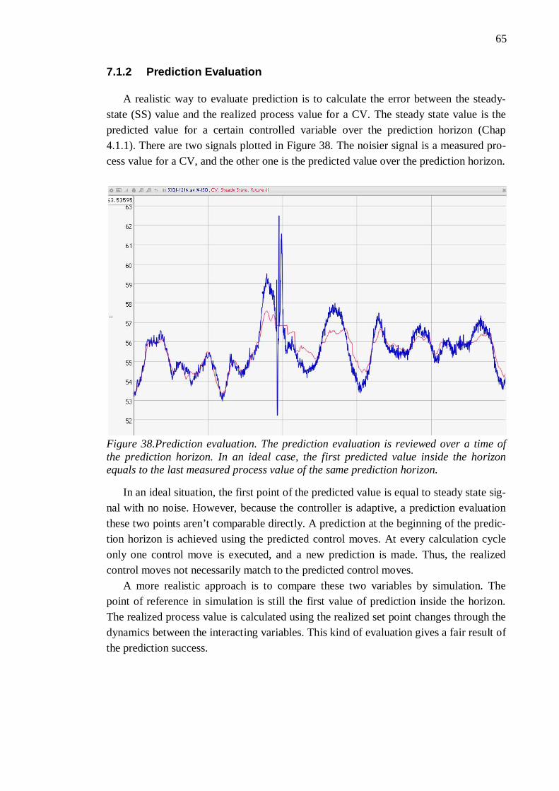
65
7.1.2 Prediction Evaluation
A realistic way to evaluate prediction is to calculate the error between the steady-state (SS) value and the realized process value for a CV. The steady state value is the predicted value for a certain controlled variable over the prediction horizon (Chap 4.1.1). There are two signals plotted in Figure 38. The noisier signal is a measured pro-cess value for a CV, and the other one is the predicted value over the prediction horizon.
Figure 38.Prediction evaluation. The prediction evaluation is reviewed over a time of the prediction horizon. In an ideal case, the first predicted value inside the horizon equals to the last measured process value of the same prediction horizon.
In an ideal situation, the first point of the predicted value is equal to steady state sig-nal with no noise. However, because the controller is adaptive, a prediction evaluation these two points aren’t comparable directly. A prediction at the beginning of the predic-tion horizon is achieved using the predicted control moves. At every calculation cycle only one control move is executed, and a new prediction is made. Thus, the realized control moves not necessarily match to the predicted control moves.
A more realistic approach is to compare these two variables by simulation. The point of reference in simulation is still the first value of prediction inside the horizon. The realized process value is calculated using the realized set point changes through the dynamics between the interacting variables. This kind of evaluation gives a fair result of the prediction success.
66
7.1.3 GUI Improvements
In addition to suggested improvements in contents, some development for the tool user interface’s features is in order. The performance monitoring user interface for a controlled variable (Fig. 20) had a changing time window that could be manually ad-justed. As well as the time window (on x-axis), the data range (y-axes) should also be user definable. For the correlation analysis it would be also valuable to add the maxi-mum delay, since at the moment correlation is evaluated over a same period of time, though the delays vary quite significantly according to which two process variables are evaluated.
7.2 Future Improvements and Product Development for MRAC
Since the implementation for model reference adaptive control fell short, it is evi-dent that the tool requires improvements. The improvements for the model reference adaptive control (MRAC) performance monitoring regards the content of the tool and developing the presentation methods of data. Other study methods would provide a use-ful addition for the tool.
7.2.1 Model Quality
The model quality for model reference adaptive control was evaluated using time se-ries analysis. One parameter of interest for monitoring is the adjustment factor (Chap 5.2), which is the constant value used to fix the control signal based on the error be-tween a reference model output and the process model output. Basically, an integrating positive or negative error between the two signals reflects that the reference model might be off, and needs to be updated.
7.2.2 Residence Time Simulation
In causticizing process, the transmission of process qualities was evaluated for ex-ample in causticizing efficiency (CE-%) control, using time series analysis. The correla-tion was determined between measured analyzer values before the first causticizing chamber, and after the last causticizing chamber. A time delay lag (Chap. 2.3.5) indi-cates that model error exists, and the model needs to be updated.
The time delay lag can be compensated by changing the residence time. The resi-dence time is related to the flow that enters the first causticizing chamber; increasing the flow means a longer residence time, and a greater total volume of the causticizing chambers. If mixing of chambers is neglected, the total volume can be used as a variable to set the correct residence time. Simulating for different causticizing chamber total volume and the corresponding residence times, the right model can be figured out and update accordingly.
67
8 SUMMARY
The final chapter of the thesis discusses the results in terms of implementing the control loop performance monitoring (CLPM).
In pulp and paper industries the processes are highly interactive and the process de-lays are quite significant. These sorts of processes are ideal for an advanced control so-lution like the model predictive control (MPC) or model reference adaptive control (MRAC) solution. For a basic regulatory controller such as the PID, monitoring a single input single output (SISO) process is quite straightforward. However, in a multivariate, highly interactive processes controlled with an advanced control solution, monitoring not only focuses on just process equipment, but also other factors like overall perfor-mance or economics. In this case the usefulness of an active CLPM is even preferred.
The number of installed control loop performance monitoring (CLPM) solutions is relatively low at the moment, although there are multiple vendors offering the software. A real time CLPM solution can reduce costs and increase profit by allowing a quick response to process variations. Consequently, it is beneficial for both the solution pro-vider as well as the customer.
In a multivariate process, a quick responding to the variations can make the differ-ence between poor and well performing process controls. It is fair to assume that a con-trol loop performance monitoring solution will provide an asset in achieving a desired performance.
The features of a CLPM solution should be relatively easy to understand. At the same time they should be informative enough, so that the process characteristics are covered. Simple configuration enables faster implementation and therefore a chance for earlier performance monitoring. A common widely recognized feature is ease of access. Thus, the solutions usually were implemented as web based service. The monitored pro-cess related KPI’s were selected based on the process experience by control engineers. The used methods for analysis were selected to meet the purposes of monitoring for the destined process.
The decision to apply the tools as a part of the existing monitoring system was fairly obvious. Like other vendor provided CLPM solutions, the tool was implemented as a browser based service. The main reason was that it enables accessing the tool relatively straightforward. The implemented control loop performance monitoring solutions were configured so that they can be applied to future MPC or MRAC cases with minor ad-justments. Performance monitoring for other multivariate control solutions are a topic of interest for future implementation.

68
Implementing control loop performance monitoring (CLPM) tool for MPC was suc-ceeded fairly good, although the MRAC case had issues which resulted complications for the implementation. The main objectives for the thesis was to determine the type of CLPM solution is needed, and to find the necessary key performance indicators (KPI’s), and the right analyzing methods, which will provide sufficient amount of information to increase control awareness, without making it too complex and difficult to understand. For future installations, the tool also needed to be relatively easy to configure.

69
REFERENCES Arpalahti, O., Engdahl, A., Jäntti, J., Kiiskilä, E., Liiri, O., Pekkinen, J., Puumalainen, R., Sankala, H., Vehmaa-Kreula, J.2002. Chemical Pulping. In:Papermaking Science and Technology. Jyväskylä, Gummerus p. B161-B173. Bethoux, G., Courtiol, C.1973. A Hyperstable Discrete Model Reference Adaptive Con-trol Systems. In: Proc 3rd IFAC Symposium on Sensitivity, Adaptivity, and Optimatily. ISA. Ischia, Italy. pp 282-289. Box G.E.P., Jenkins, G.M., 1970, Time Series Analysis Forecasting and Control, Hold-en-Day, Inc. San Francisco, CA Cameron, C., Windmeijer, F. (1996) An R-squared measure of goodness of fit for some common nonlinear regression models. Journal of Economics, Volume 77, Issue 2, pages 329-342. Clarke, D.W., Mohtadi, C., Tuffs, P.S.1987.Generalized Predictive Control Part 1. The Basic Algorithm. Automatica Vol. 23 No 2. p.137-148 Cryer, J. D., Chan, K-S.2008. Time Series Analysis with Applications 2nd Edition. Springer Science+ Business Media. New York, NY Cutler, C. R., Ramaker, B. L.1979. Dynamic Matrix Control – a Computer Control Al-gorithm. American Institute of Chemical Engineers 86th National Meeting. Houston,TX Dorf, R.C., Bishop, R.H.2000. Moderen Control Systems 9th Edition. Prentice Hall. New Jersey, USA Feldbaum, A. 1965. Optimal Control Theory. Academic Press. New York Griva, I., Nash, S.G,Sofer, A.2009. Linear and Nonlinear Optimization. 2nd Edition. USA, Society for Industrial and Applied Mathematics p. 10-11 Hedengren, J. D., Allsford, K. V., Ramlal, J.2007. Moving Horizon Estimation and Control for an Industrial Gas Phase Polymerization Reactor. Published in Proceedings of American Control Conference (ACC). New York History Monitoring. Public Domain Release [WWW].Expertune.2014.[referred 17.10.2014].Available: http://www.expertune.com/PTTrends.aspx
70
Holik, H.2000. Recycled Fiber and Deinking. In:Papermaking Science and Technology Chap. 5 p. 91-204 . Jyväskylä, Gummerus. Hunter, J.D., 2007. Matplotlib: A 2D graphics environment. Published in Computing In Science & Engineering. Vol. 9 No. 3 USA. IEEE Computer Society. p. 90-95 Hägglund, T.1992. Disturbance supervision in feedback loops. In Tooldiag’93 Interna-tional Conference on Fault Diagnosis. Toulouse, France IMAS. Metso Public Domain Release [WWW]. Metso.2013. [referred 6.9.2013]. Avail-able: http://www.metso.com/automation/pp_prod.nsf/WebWID/WTB-050630-2256F-77478?OpenDocument#.UinLBDbxrTg IMON. Metso Public Domain Release [WWW]. Metso.2013. [referred 6.9.2013]. Available: http://www.metso.com/automation/pp_prod.nsf/WebWID/WTB-050630-2256F-9BBB2#.UinQRDbxrTg Interaction Map. Public Domain Release [WWW].Expertune.2014.[referred 31.3.2014].Available: http://www.expertune.com/PTInteractionMap.aspx James, G. Advanced Modern Engineering Mathematics. 3rd Edition. Harlow. Pearson Education Limited. p. 364-369 Kraus, T.W., Myron, T.J.1984. Self-tuning pid controller uses pattern recognition ap-proach. Control Engineering 31. p.106-111 Landau, I.D. 1971. Synthesis of a Discrete Model Reference Adaptive Systems. IEEE Transactions on Automatic Control AC-16:507-508 Lane, D.2013. Online Statistics Education, Introduction to linear regression theory [WWW] Available: http://onlinestatbook.com/2/regression/intro.html [referred 6.6.2014] Lassus, A.2000. Recycled Fiber and Deinking. In:Papermaking Science and Technology Chap. 5 p. 241-245. Jyväskylä, Gummerus. Ljung, L. and Z.D. Yuan (1985). Asymptotic Properties of Black-box Identification of Transfer Functions. IEEE Trans. Autom. Control, Vol. AC-30, p.514-530. Lutz, M. 2000. Learning Python. 4th Edition. Sebastopol, USA. O’Reilly Media Inc. p. 11
71
Lynch, C.1992. Control Loop Performance Monitoring. Maciejowski, J. M., 2002. Predictive Control with Constraints. Prentice Hall, ISBN 0-201-39823-0 Process Monitoring. Solutions Public Domain Release [WWW]. ABB.2013. [referred 5.9.2013]. Available: http://www05.abb.com/global/scot/scot281.nsf/veritydisplay/6d34b71f04b48b2ec1257537003cf73c/$file/fujairah_pr_deabb%201236%2005_e_big.pdf Qin, S. J.,Badgwell, T. A.2003. A Survey of Industrial Model Predictive Control Tech-nology. Control Engineering Practice Vol. 11 No. 7. p. 503-507 Richalet, J., Rault, A., Testud, J. L., Papon, J.1978. Model Predictive Heuristic Control: Applications to Industrial Processes. Automatica Vol. 14 No 5. p.413-428 Smuts, J. F., Sorge, J. N., Evely, D., Faurot, M., Hussey, A2011. Control Loop Perfor-mance Monitoring in a Power Plant. Presented at the 2011 ISA Power Industry Division Symposium Software Sensor. Metso Public Domain Release [WWW]. Metso.2013. [referred 6.9.2013]. Available http://www.metso.com/automation/pp_prod.nsf/WebWID/WTB-050630-2256F-70E2C?opendocument#.UinQbjbxrTg TaiJi. Public Domain Release [WWW].Matrikon.2014.[referred 31.3.2014].Available: http://www.matrikon.com/control-performance-monitoring/taiji-apc.aspx Tolonen, J., Tolonen, O., Puhakka, J.2002. Optimisation of the causticising process. TAPPSA Journal.Vol. 02. No. 7. Visioli, A.2003. Modified anti-windup scheme for PID controllers. Julkaistu: IEEE Control Theory and Applications Vol. 150 No 1. s. 49-54 Whitaker, H.P. An Adaptive System for Control of the Dynamics Performances of Air-craft and Spacecraft. 1959. Institute of Aeronautical Services, Paper 59-100 Zhu, Y.C. (1989). Black-box Identification of MIMO Transfer Functions: Asymptotic Properties of Prediction Error Models. Int. J. Adaptive Control and Signal Processing, Vol. 3, p. 357-373.