Intelligent modeling and identification of aircraft

Chinese Journal of Aeronautics, (2014),27(4): 759–771

Chinese Society of Aeronautics and Astronautics& Beihang University

Chinese Journal of Aeronautics

[email protected]

Intelligent modeling and identification of aircraft

nonlinear flight

* Corresponding author.E-mail addresses: [email protected] (A. Roudbari),

[email protected] (F. Saghafi).

Peer review under responsibility of Editorial Committee of CJA.

Production and hosting by Elsevier

http://dx.doi.org/10.1016/j.cja.2014.03.0171000-9361 ª 2014 Production and hosting by Elsevier Ltd. on behalf of CSAA & BUAA.Open access under CC BY-NC-ND license.

Alireza Roudbari *, Fariborz Saghafi

Department of Aerospace Engineering, Sharif University of Technology, 14588 Tehran, Iran

Received 28 June 2013; revised 30 August 2013; accepted 15 November 2013

Available online 4 May 2014

KEYWORDS

Flight test;

Genetic algorithms;

Nonlinear flight dynamics;

Nonlinear system

identification;

Recurrent neural network

Abstract In this paper, a new approach has been proposed to identify and model the dynamics of

a highly maneuverable fighter aircraft through artificial neural networks (ANNs). In general, air-

craft flight dynamics is considered as a nonlinear and coupled system whose modeling through

ANNs, unlike classical approaches, does not require any aerodynamic or propulsion information

and a few flight test data seem sufficient. In this study, for identification and modeling of the aircraft

dynamics, two known structures of internal and external recurrent neural networks (RNNs) and a

proposed structure called hybrid combined recurrent neural network have been used and compared.

In order to improve the training process, an appropriate evolutionary method has been applied to

simultaneously train and optimize the parameters of ANNs. In this research, it has been shown that

six ANNs each with three inputs and one output, trained by flight test data, can model the dynamic

behavior of the highly maneuverable aircraft with acceptable accuracy and without any priori

knowledge about the system.ª 2014 Production and hosting by Elsevier Ltd. on behalf of CSAA & BUAA.

Open access under CC BY-NC-ND license.

1. Introduction

Modeling and simulation are widely used as essential tools to

predict and analyze complex systems in various scientific andengineering fields. For an aerospace system such as an aircraft,mathematical models can serve as useful tools in flight simula-tion, dynamic analysis, controller design, as well as navigation

and guidance studies. Aircraft models can be determined intwo different ways. The first approach is a theoretical (classi-cal) method using the basic laws of physics such as Newton–

Euler and Lagrange–Euler equations to describe aircraftdynamic behaviors.1,2 The second approach is based on exper-imental identification of aircraft dynamics using a wind tunnel

and flight test data. The theoretical modeling of an aircraftrequires some types of data including aerodynamic, inertial,and structural properties of various elements of the airframe.

These data are not always accurate enough and their computa-tions are often costly and in some cases, even unavailable.These models are usually linearized or only valid in a limitedboundary around a specific point. Furthermore, when the

degree of nonlinearity increases, the modeling process becomeseven more difficult.

http://crossmark.crossref.org/dialog/?doi=10.1016/j.cja.2014.03.017&domain=pdf

mailto:[email protected]

mailto:[email protected]

http://dx.doi.org/10.1016/j.cja.2014.03.017


http://www.sciencedirect.com/science/journal/10009361


http://creativecommons.org/licenses/by-nc-nd/4.0/

http://creativecommons.org/licenses/by-nc-nd/4.0/

760 A. Roudbari, F. Saghafi

Identification methods which work based on the measure-ment of the whole system input/output can serve as betterand faster approaches for complicated systems such as aircraft

in order to obtain accurate models.3 So far, various methodsfor system identification have been applied, some of whichare introduced in the Refs.3–6. The frequency domain analy-

sis,7,8 the fuzzy identification,9–11 the state space identifica-tion,12,13 and the artificial neural networks (ANNs)14–16 areamong the most renowned methods.

ANNs are a new approach for modeling and identificationof systems which are called ‘‘intelligent techniques’’. They havebeen of great interest to many researchers over the past twodecades.17 ANNs’ applications have mostly been in various

domains of aeronautics. In this regard, modeling of linearizedlateral aircraft dynamics,18,19 estimation of aerodynamic forcesand moments acting on aircraft,20 and controllers design21–23

can be mentioned. In majority of these applications, onlineidentification has been usually performed; while the networkis running, ANN training would continue. Therefore, it can

be said that generalization loses its significance. Due to generalapproximation and generalization capabilities, ANNs arepotentially applicable to offline nonlinear modeling of aircraft

dynamics for simulation purposes.In the present study, a new ANN approach has been pro-

posed to model the coupled nonlinear six-degree-of-freedomdynamics of a highly maneuverable aircraft. For this purpose,

three different types of ANN architectures including the non-linear output error structure (NNOE),24,25 neural networknonlinear autoregressive with exogenous (NNARX),26 and

partially internal recurrent networks proposed by Elman27

and Jordan28 have been used and compared. Moreover, inorder to increase the memory capacity and obtain better per-

formance in ANNs for modeling and identification, a newtopology of partially internal recurrent networks called hybridcombined recurrent network has been introduced and com-

pared with the previous structures.Although ANNs have been extensively applied in various

areas of science, no efficient method has so far been proposedfor optimization of ANN parameters. The network size, type

of ANN topology, and suitable training algorithms play themost important roles for better learning and generalizationof ANNs. Larger networks have faster training; however, their

generalization is worse, whereas smaller ones have better gen-eralization with slower learning. In order to obtain smaller net-works, Sexton proposed a method for feedforward networks

called ANN simultaneous optimization algorithm(NNSOA).29 This method applies a genetic algorithm (GA)to simultaneously train and find a parsimonious ANN archi-tecture. In this study, a similar algorithm has been used and

developed for training recurrent neural networks (RNNs) inorder to identify and model aircraft nonlinear dynamics. Inorder to show its effectiveness in improving generalization of

ANNs, the proposed algorithm is then compared with the ori-ginal genetic algorithm.

2. Data generation

In order to show ANNs’ abilities in modeling and identifica-tion, three sets of data have been used:�1 Linear and decou-

pled dynamics of the Beech M99 and F-4D fighter aircraft.�2 Nonlinear six-degree-of-freedom model of the F-16 fighter

aircraft dynamics.�3 Experimental measurements of a highlymaneuverable 4th generation fighter aircraft.

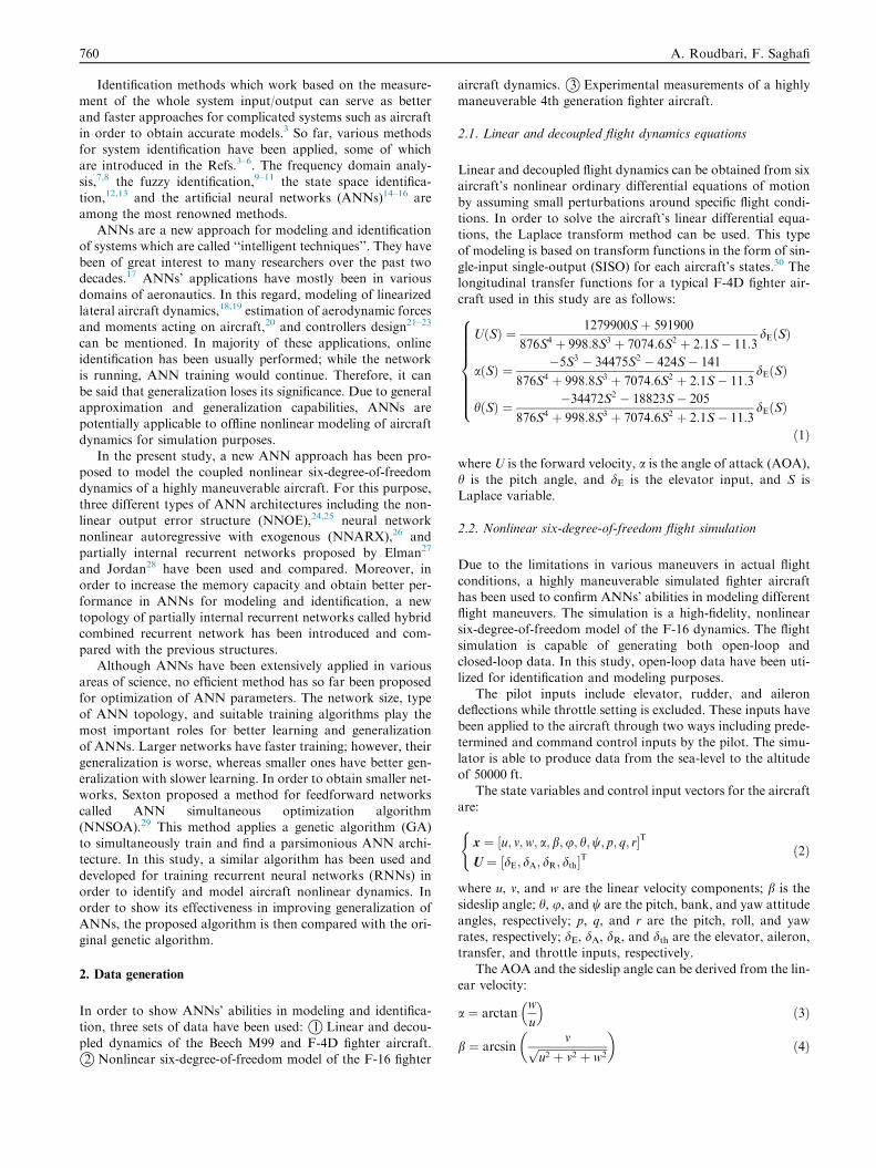
2.1. Linear and decoupled flight dynamics equations

Linear and decoupled flight dynamics can be obtained from sixaircraft’s nonlinear ordinary differential equations of motion

by assuming small perturbations around specific flight condi-tions. In order to solve the aircraft’s linear differential equa-tions, the Laplace transform method can be used. This type

of modeling is based on transform functions in the form of sin-gle-input single-output (SISO) for each aircraft’s states.30 Thelongitudinal transfer functions for a typical F-4D fighter air-

craft used in this study are as follows:

UðSÞ ¼ 1279900Sþ 591900

876S4 þ 998:8S3 þ 7074:6S2 þ 2:1S� 11:3dEðSÞ

aðSÞ ¼ �5S3 � 34475S2 � 424S� 141

876S4 þ 998:8S3 þ 7074:6S2 þ 2:1S� 11:3dEðSÞ

hðSÞ ¼ �34472S2 � 18823S� 205

876S4 þ 998:8S3 þ 7074:6S2 þ 2:1S� 11:3dEðSÞ

8>>>>>>><>>>>>>>:ð1Þ

where U is the forward velocity, a is the angle of attack (AOA),h is the pitch angle, and dE is the elevator input, and S isLaplace variable.

2.2. Nonlinear six-degree-of-freedom flight simulation

Due to the limitations in various maneuvers in actual flight

conditions, a highly maneuverable simulated fighter aircrafthas been used to confirm ANNs’ abilities in modeling differentflight maneuvers. The simulation is a high-fidelity, nonlinear

six-degree-of-freedom model of the F-16 dynamics. The flightsimulation is capable of generating both open-loop andclosed-loop data. In this study, open-loop data have been uti-

lized for identification and modeling purposes.The pilot inputs include elevator, rudder, and aileron

deflections while throttle setting is excluded. These inputs havebeen applied to the aircraft through two ways including prede-

termined and command control inputs by the pilot. The simu-lator is able to produce data from the sea-level to the altitudeof 50000 ft.

The state variables and control input vectors for the aircraftare:

x ¼ ½u; v;w; a; b;u; h;w; p; q; r�T

U ¼ ½dE; dA; dR; dth�T

(ð2Þ

where u, v, and w are the linear velocity components; b is the

sideslip angle; h, u, and w are the pitch, bank, and yaw attitudeangles, respectively; p, q, and r are the pitch, roll, and yawrates, respectively; dE, dA, dR, and dth are the elevator, aileron,transfer, and throttle inputs, respectively.

The AOA and the sideslip angle can be derived from the lin-ear velocity:

a ¼ arctanw

u

� �ð3Þ

b ¼ arcsinvffiffiffiffiffiffiffiffiffiffiffiffiffiffiffiffiffiffiffiffiffiffiffiffiffi

u2 þ v2 þ w2p� �

ð4Þ

Intelligent modeling and identification of aircraft nonlinear flight 761

The time-derivative of the quaternion can be expressed as

follows:

_q

_q1

_q2

_q3

2666437775 ¼ 1

2

0 �p �q �rp 0 r �qq �r 0 p

r q �p 0

2666437775

q0

q1

q2

q3

2666437775 ð5Þ

where q0, q1, q2, and q3 are the quaternion elements.The Euler angles can now be derived from the Eq. (2) as the

following:

w ¼ arctan2ðq1q2 þ q0q3Þ

q21 þ q21 � q22 � q23

� �h ¼ arcsin½�2ðq1q3 � q0q2Þ�

u ¼ arctan2ðq2q3 þ q0q1Þ

q20 � q21 � q22 þ q23

� �8>>>>><>>>>>:

ð6Þ

The aerodynamic is modeled by calculating the non-dimen-

sional forces and moment coefficients which, as presented inthe following equations, vary nonlinearly based on the AOA(within �10� 6 a 6 45�) and the sideslip angle (within

�30� 6 b 6 30�), the angular velocities (p, q, r), and the con-trol surface deflections (dE, dR, and dA). In these equations,any of damping and control derivatives can be obtained by

interpolating through tabular aerodynamic data.The non-dimensional forces and moment coefficients are

Cl, Cm, Cn, Cx, Cy, and Cz which have been resulted fromthe following equations:

Cx¼CxqðaÞqþCxp ða;dEÞCy¼CypðaÞqþCyrðaÞrþð�0:02bþ0:00287dRþ0:0105dAÞ

Cz¼CzqðaÞqþSðaÞ 1�ðb=57:3Þ2� �

�0:19ðdE=25ÞCl¼ClpðaÞpþClrðaÞrþCldA

ða;bÞdAþCldRða;bÞdRþClqða;bÞ

Cm¼CmqðaÞqþCmp

ða;dEÞCn¼CnqðaÞpþCnrðaÞrþCndA

ða;bÞdAþCndRða;bÞdRþCnða;bÞ

8>>>>>>>>>><>>>>>>>>>>:ð7Þ

where Cxp ; Cxq ; Cyp ; Cyr ; Czq ; Cmp; Cmq

; Clr ; Clp ; Clq ; Cnq ;Cnr ; CndA

are damping derivatives and CldA, CldR

;CndAand

CndEare control derivatives.

The forces and moments of the aircraft in the body framesystem are calculated using the following equations:

½fa;p�B ¼fa;p1

fa;p2

fa;p3

264375 ¼ �qsCx þ fp

�qsCy

�qsCz

264375 ð8Þ

½mB�B ¼mB1

mB2

mB3

264375 ¼ �qsbCl

�qscCm

�qsbCn

264375 ð9Þ

where fa,p and mB are the total aerodynamic and propulsionforce and moment vectors in the body axes; s, b, and c are

the wing area, the wing span, and the mean aerodynamicchord, respectively; �q is dynamic pressure.

Applying Euler and Newton laws leads to the following six

first-order coupled nonlinear ordinary differential equationswhich have been numerically solved through the fourth-orderRunge–Kutta method for p, q, and r.

_p ¼ 1=I11I13 þ I213 I2I33 � I233 � I213

r� I13ðI33��

þI11 � I2Þp� I13lR�qþ I33mB1 � I13mB3g

_q ¼ 1=I2f½ðI33 � I11Þp� lR�rþ I13ðp2 � r2Þ þmB2g

_r ¼ 1=I11I13 þ I213 ð�I2I11 þ I211 þ I213Þp� I13ðI33 þ I11�

�I2Þrþ I11lR�qþ I11mB3 � I13mB1

_u ¼ rv� qwþ fa;p1=mþ 2ðq1q3 � q0q2Þg

_v ¼ pw� ruþ fa;p2=mþ 2ðq2q3 þ q0q1Þg

_w ¼ qu� pvþ fa;p3=mþ ðq20 � q21 � q22 þ q23Þg

8>>>>>>>>>>>>>>>>>>>><>>>>>>>>>>>>>>>>>>>>:

ð10Þ

where I11, I2, I33, I13 are the elements of the inertia moments

matrix; lR is the engine angular momentum and _u; _v; _w arethe translational accelerations in the body axes.

3. Experimental data

The experimental data were extracted from a 4th generationfighter aircraft called X-craft in this study. This aircraft is

equipped with two gas-turbine jet engines, and benefits froma superior thrust/weight ratio and excellent aerodynamics.The aircraft’s primary flight controls consist of the elevator,

the rudder, and the aileron. Longitudinal control is providedby the synchronized deflection of the elevator. Lateral controlis provided mainly by the aileron and by the rudder at a high

AOA. The aircraft is stabilized with a highly augmented feed-back control law. It should be mentioned that the open-loopaircraft is unstable in high AOA flight conditions.

The flight tests were performed in calm weather at a specific

Mach and altitude (so-called trim point). For this purpose, theaircraft was trimmed in straight and level flight conditions at aMach of 0.65 and a altitude of 11000 ft. To obtain proper

flight data, all control inputs were applied to the aircraftaround the trim point. However, due to the high maneuver-ability of the aircraft during the flight tests, Mach and altitude

were changed within the range of 0.4–0.80 and 10000–12000 m,respectively. All the control inputs were manually inserted bythe pilots. In order to obtain proper data, the pilots manually

applied suitable inputs to each aircraft’s control surface sepa-rately. For example, while the pilot was moving the stick tochange dA, the other control surfaces including dE and dRshould remain constant in their initial conditions.

The aircraft was instrumented to measure longitudinal (nx),lateral (ny), and normal (nz) translational accelerations, pitch(h), roll (/), yaw angle (w), indicated airspeed (v), barometric

altitude (h), and AOA. The signals were sampled at 10 Hzand stored on an on-board flight data recorder (FDR). TheFDR device recorded both the pilot inputs applied by the stick

and the control surface changes. If the aircraft control surfacechanges are fed into the network as input training, the ANNwill learn the aircraft dynamic behavior as open-loop, whereasif the pilot inputs applied by the stick are fed into the network,

the network will learn the aircraft dynamic behavior as closed-loop.

Fig. 1 shows the multi-step signal for actual flight tests on

the three aircraft inputs including elevator, aileron, and rud-der, which have been used for ANN training.

Fig. 1 Training input signals used in actual flight tests.


4. Training input signal

The type of input (excitation) signals is very important in col-lecting identification data for ANNs training process. In flying

vehicles such as fighter aircraft, the input signals should beable to excite various dynamic modes. The standard multi-stepDLR3211 (see Fig. 2) and sweep frequency are two of the

known input signals which are suitable for aircraft identifica-tion. These inputs have been proved to be very effective inexciting aircraft flight dynamic modes.5,31

Multi-step DLR3211 signals were chosen as the networktraining inputs for each of the aircraft’s three inputs. Thesethree inputs can be fed into the network in a series manner.

In this way, the input neurons, related to each one of the con-trol inputs, are excited for about 6 s by the DLR3211 signalaround the trim point while the other two input neuronsremain constant in their initial trim points. Therefore, the total

time to apply the inputs will be 18 seconds.To obtain linear decoupled flight dynamic data, the input

DLR3211 has been defined in the form of Laplace transfer

function. For example, the Laplace transfer function of dR(s)which has been used in this study is as follows:

dRðSÞ ¼0:1e�2S � 0:2e�8S þ 0:2e�12S � 0:2e�14S þ 0:1e�16S

S

ð11Þ

By putting dR(S) or dE(S) in the aircrafts’ transfer functionscalculating the inverse Laplace, the states of b(t), w(t), /(t),a(t), and h(t) in longitudinal and lateral directions will be

obtained.

5. Neural network architectures

ANNs for system identification can be considered as ‘‘blackbox’’ models which have a number of parameters that canadapt themselves in response to system variations. The

Fig. 2 Training input of DLR3211 used in F-16 flight simulator.

behavior of the network depends on the relations betweenthe layers and the weights working in unison to solve particu-lar problems. Based on this, a variety of ANN architectures

have been proposed, of which the feedforward and recurrentnetworks are the main ones for ANNs used for dynamic sys-tem identification. The multi-layered feedforward networks,

known as perceptron, are the most frequently used structuresin ANNs which are capable of extrapolation and interpolation.However, these types of ANNs are unable to determine time

effect. Therefore, they are not suitable for modeling and iden-tification of dynamic systems. By adding input history and out-put feedback as the inputs to feedforward ANNs, the dynamicmemory capacity of ANNs increases and therefore, they

become suitable for nonlinear dynamics identification. Thesetypes of ANNs have come to be known as time delayed neuralnetworks (TDNNs).32 The TDNNs are the multi-layer net-

works of perceptron that have time-delayed recurrent connec-tions which can be internal or external.

5.1. External recurrent neural networks

NNARX and NNOE are the most common external RNNs.NNARX is a recurrent dynamic network, with external feed-

back connections including several layers of the network. Inthis network, the system’s outputs have been used as the input.Thus, this network is known as a series–parallel network. Thenetwork output can be described as:

yn¼ fðuðkÞ;uðk�1Þ; . . . ;ypðkÞ;ypðk�1Þ; . . . ;ypðk� jþ1ÞÞ ð12Þ

This structure can be applied as a predictor to predict one

step ahead of the input signal. It can also be used for the mod-eling of nonlinear dynamic systems.24 The input regression sig-nal vector includes. The new and previous values of the system

input: [U(t), U(t � 1), . . . , U(t � i + 1)]. It demonstrates theindependent (exogenous) network input signal. The new andprevious values of the system output: [Yp(t � 1),Yp

(t � 2), . . . ,Yp (t � j + 1)]. This is the output regression vectorof the system. Therefore, the network regression vector is:

wuyðkÞ ¼ ½Uðk� 1Þ;Uðk� 2Þ; . . . ;Uðk�mþ 1Þ;Yðk� 1Þ;Yðk� 2Þ; . . . ;Ypðk� jþ 1Þ�T ð13Þ

In a two-layered NNARX network, by applying a tangent

sigmoid bipolar transfer function in the first layer and a lineartransfer function in the second layer; the equations of the net-work are as follows:

bY1l ðkÞ ¼ tansig ðIW1 �Uðk� 1Þ þ IW2 �Uðk� 2Þþ; . . . ; IWi

�Uðk� iþ 1Þ þ b1 þOW1 � bYnðk� 1Þ þOW

2

� bYnðk� 2Þþ; . . . ;OWj � bYnðk� jþ 1ÞÞ ð14Þ

bY2nðkÞ ¼ purlin ðLW� bY1

l ðkÞ þ b2Þ ð15Þ

where IWi, LW, OWj, b1, and b2 are the weight matrices of the

input to the hidden layer, the hidden layer to the output layer,the context unit of the middle layer, the self-feedback of themiddle context unit, and the bias vectors of the hidden and

output layers, respectively; U is the input vector of theANN; bY1

l is the output vector of the hidden layer; bY2n is the

output of the ANN. and i, j are the number of additionalself-feedback connections for each neuron.


This model is similar to NNARX with the only differencethat the network outputs are fed back as input to the network.This structure is suitable for offline identification and multi-

step ahead prediction. The network regression vector is:

wuyðkÞ ¼ ½Uðk� 1Þ;Uðk� 2Þ; . . . ;Uðk� iþ 1Þ; bYnðk� 1Þ;bYnðk� 2Þ; . . . ; bYnðk� jþ 1Þ�T ð16Þ

The equations used in this network are as the following:

bY1l ðkÞ ¼ tansig ðIW1 �Uðk� 1Þ þ IW2 �Uðk� 2Þþ; . . . ; IWi

�Uðk� iþ 1Þ þ b1 þOW1 � bYpðk� 1Þ þOW

2

� bYpðk� 2Þþ; . . . ;OWj � bYpðk� jþ 1ÞÞ ð17Þ

bY2nðkÞ ¼ purlin LW� bY1

l ðkÞ þ b2� �

ð18Þ

5.2. Internal recurrent neural network

RNNs can be classified into two main architectures: fully andpartially RNNs. In fully RNNs, the outputs of all neurons arerecurrently connected to all neurons in the network. In par-

tially RNNs, a set of additional connections is added to theinput layer that receives the input from the hidden or outputneuron layers. A special case of the partially RNN architecture

was employed by Elman27 and Jordan.28 Elman and Jordan’snetworks are also known as simple recurrent networks(SRN). The Elman network is commonly a two-layer networkwith feedback from the first-layer outputs to the first-layer

inputs called context units. These units are hidden becausetheir neurons only interact exclusively with the internal neu-rons of the network and are not connected to the outside

world. Context neurons are recurrent and representative ofthe internal states, because they provide feedback from themiddle-layer output to the network as input, i.e., these neurons

use the previous states as the input. That is, the context unitsstore the system’s previous states which are adjusted by weightmatrices (CW). In this network, the context neurons save thelast state’s value of the middle layer. Thus, the context neurons

can remember the previous internal state. Hidden layers enablethe network to produce the desired output for any given maininputs. Therefore, the hidden layers with context units have the

task of mapping both an external input and the previous inter-nal state to desired outputs; as a result, the network under-stands time effect in the process.27

The network structure acts as a multi-layered networkwhose input layer consists of external inputs (inputs of the sys-tem) and the outputs of the context units neurons

(Uc1 ¼ Cl1; Cl2; . . . ;ClL½ �TÞ. Hence, the external inputsof the network and the outputs of the context neurons createa new input vector known as U.

U ¼ U1; U2; . . . ; UI; Cl1; Cl2; . . . ; ClL½ �T ð19Þ

The equations of this network by applying a tangent sig-moid bipolar transfer function in the first layer and a linear

transfer function in the second layer are as follows:bY1l ðkÞ ¼ tansig IW1 �Uþ b1 þ CW

1 � Y1l ðk� 1Þ

ð20ÞbY2

nðkÞ ¼ purlin LW� bY1l ðkÞ þ b2

� �ð21Þ

The modified Elman network (see Fig. 3) is the same as theElman network; the only difference is that self-recurrent ele-ments have been added to each neuron of the context unit

within the middle layer to increase the dynamic memory.33

For example, when each neuron is fed back to itself twice,the following term is added to the network equations:

CW2 � bY1

1ðk� 2Þ þ CW3 � bY1

1ðk� 3Þ ð22Þ

This process makes the ANN model capable of predicting

the dynamic systems more accurately, especially when theinputs remain constant for a long period of time. Thus, theequations used for this network are as follows:

bY1l ðkÞ ¼ tansig IW�UðkÞ þ b1 þ CW1 � bY1

l ðk� 1Þ þ CW2�

� bY1l ðk� 2Þ þ b2 þ CW

3 � bY1l ðk� 3Þ

�ð23Þ



ð24Þ

The Jordan network is similar to the Elman network. How-ever, instead of the hidden layer, the context units are fed fromthe output layer. The context units in the Jordan network arealso referred to as the state layer. This network can also be

modified by additional self-feedback connections to each neu-ron in order to increase the dynamic memory. The equationsused in this network are as follows:

bY1l ðkÞ¼ tansig IW1�Uþb1þJW1� bY2

nðk�1ÞþJW2� bY2nðk�2Þ

� �ð25Þ

bY2nðkÞ¼ purlin LW� bY1

l ðkÞþb2� �

ð26Þ

where JW1 is the weight matrix of the context unit in the out-put layer and JW2 is the weight matrix of the self-feedback in

the output context unit.

5.3. Hybrid combined recurrent network

In the Elman and Jordan networks, context units only exist inone of the network layers. To increase the dynamic capacity,context units can be created in all the network layers. This pro-

posed network has been named hybrid combined recurrentnetwork. In this network, there are two context units calledthe middle and output context units. This network consists

of two parts. The first part is a multi-layer forward network,

Fig. 3 Modified Elman network architecture.

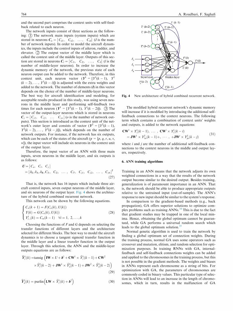
Fig. 4 New architecture of hybrid combined recurrent network.


and the second part comprises the context units with self-feed-back related to each neuron.

The network inputs consist of three sections as the follow-

ing: �1 The network main inputs (system inputs) which arestored in neurons Cu ¼ ½Cu1; Cu2; . . . ; CuI� (I is the num-ber of network inputs). In order to model the aircraft dynam-

ics, the inputs include the control inputs of aileron, rudder, andelevator. �2 The output vector of the middle layer which iscalled the context unit of the middle layer. Outputs of this sec-

tion are stored in neurons Cl ¼ ½Cl1; Cl2; . . . ; Cll� (l is thenumber of middle-layer neurons). In order to increase thedynamic memory of the network, the previous state of eachneuron output can be added to the network. Therefore, in this

context unit, each neuron vector (Y1 = [Y1(k � 1), Y1

(k � 2), . . . , Y1(k � i)]) is adjusted with the extra weights andadded to the network. The number of elements (l) in this vector

depends on the choice of the number of middle-layer neurons.The best way for aircraft identification and modeling, foracceptable results produced in this study, was using seven neu-

rons in the middle layer and performing self-feedback twotimes for each neuron (Y1 = [Y1(k � 1), Y1(k � 2)]). �3 Thevector of the output-layer neurons which is stored in neurons

Cy ¼ ½Cy1; Cy2; . . . Cyo � (o is the number of network out-puts). This section is introduced as the context unit of the net-work’s outer layer and consists of vector (Y2 = [Y2(k � 1),Y2(k � 2), . . . , Y2(k � j)]), which depends on the number of

network outputs. For instance, if the network has six outputs,which can be each of the states of the aircraft (y = [p, q, r, u, v,w]), the input vector will include six neurons in the context unit

of the output layer.Therefore, the input vector of an ANN with three main

inputs, seven neurons in the middle layer, and six outputs is

as follows:

U¼ Cu; Cl; Cy½ �¼ dE;dA;dR;Cl1; Cl2; . . . ; Cl7; Cy1; Cy2; . . . ; Cy6½ �T

ð27Þ

That is, the network has 16 inputs which include three air-

craft control inputs, seven output neurons of the middle layer,and six neurons of the output layer. Fig. 4 shows the architec-ture of the hybrid combined recurrent network.

This network can be shown by the following equations.

Cnðkþ 1Þ ¼ FðCnðkÞ;UðkÞÞYðkÞ ¼ GðCnðkÞ;UðkÞÞY1

l iðkÞ ¼ Cniðk� 1Þ 8i ¼ 1; 2; . . . ; k

8><>: ð28Þ

Choosing the functions of F and G depends on selecting thetransfer functions of different layers and the architectureselected for different blocks. The best way to model the aircraft

dynamics is to choose a tangent sigmoid transfer function inthe middle layer and a linear transfer function in the outputlayer. Through this selection, the ANN and the middle-layer

outputs equations are as follows:

bY1l ðkÞ ¼tansig IW�Uþ b1 þCW1 � bY1

l ðk� 1Þ þCW2�

� bY2l ðk� 2Þ þ JW1 � bY2

nðk� 1Þ þ JW2 � bY2nðk� 2Þ

�ð29Þ



ð30Þ

The modified hybrid recurrent network’s dynamic memory

will increase if it is modified by introducing the additional self-feedback connections to the context neurons. The followingterm which contains a combination of context units’ weights

and outputs, is added to the network equations:

CW1 � Y1

1ðk� 1Þ; . . . ; CWi � Y11ðk� iÞ

¼ JW1 � Y21nðk� 1Þþ; � � � ; þJWj � Y2

jnðk� jÞð31Þ

where i and j are the number of additional self-feedback con-nections to the context neurons in the middle and output lay-ers, respectively.

6. ANN training algorithms

Training in an ANN means that the network adjusts its own

weighted connections in a way that the results of the networkoutput become similar to the desired output. Besides training,generalization is of paramount importance in an ANN. That

is, the network should be able to produce appropriate outputsrelative to the untrained input (out-of-sample). The ANN’sresponse to new input should be similar to the system’s response.

In comparison to the gradient-based methods (e.g., back

propagation), GA offers superior solutions to optimize com-plex problems such as training ANNs.34 This is due to the factthat gradient studies may be trapped in one of the local min-

ima. Hence, obtaining the global optimum cannot be guaran-teed, while GA performs a universal random search whichleads to the global optimum solution.35

Normal genetic algorithm is used to train the network byfinding a global optimum set of connection weights. Duringthe training process, normal GA uses some operators such ascrossover and mutation, elitism, and random selection for opti-

mization purposes. In training RNNs with GA, internal-feedback and self-feedback connections weights can be addedand applied to the chromosomes in the training process, but this

is not possible in the gradient methods. The weights and biasesin ANNs represent each chromosome as a string of bits. Foroptimization with GA, the parameters of chromosomes are

commonly coded in binary values. This particular type of selec-tion in ANNs will lead to an increase in the length of chromo-somes, which in turn, results in the malfunction of GA


operators. Therefore, to avoid such drawbacks, it would be bet-ter to use decimal values in chromosomes. For example, if in themodified Elman network, the number of inputs is n, the number

of neurons is h in the hidden layer, and the number of outputs ism, then chromosomes will be shown as the following string.

ð32Þ

NNSOA is similar to GA which simultaneously trains andfinds a parsimonious structure for ANNs. For this purpose, anew operator called mutation2 (Pm2) is utilized in NNSOA

which randomly nullifies some weights and rules them out with

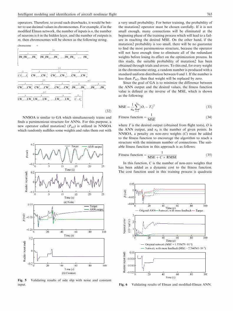
Fig. 5 Validating results of side slip with noise and constant

input.

a very small probability. For better training, the probability ofthe mutation2 operator must be chosen carefully. If it is notsmall enough, many connections will be eliminated at the

beginning phase of the training process which will lead to a fail-ure in reaching the desired MSE. On the other hand, if themutation2 probability is too small, there will be no guarantee

to find the most parsimonious structure, because the operatorwill not have enough time to eliminate all of the redundantweights before losing its effect on the optimization process. In

this study, the suitable probability of mutation2 has beenobtained through trials and errors. To this end, for every weightin the chromosome string, a random number is produced with astandard uniform distribution between 0 and 1. If the number is

less than Pm2, then that weight will be replaced by zero.Since the goal of GA is to minimize the difference between

the ANN output and the desired values, the fitness function

value is defined as the inverse of the MSE, which is shownas the following:

MSE ¼ 1

nd

Xndi¼1ðOi � TiÞ2 ð33Þ

Fitness function ¼ 1

MSEð34Þ

where T is the desired output (obtained from flight tests), O isthe ANN output, and nd is the number of given points. InNNSOA, a penalty on non-zero weights (C) must be added

to the fitness function to encourage the algorithm to reach astructure with the minimum number of connections. The suit-able fitness function in this approach is as follows:

Fitness function ¼ 1

MSEþ C�RMSEð35Þ

In this function, C is the number of non-zero weights that

has been added as a dynamic cost to the fitness function.The cost function used in this training process is quadratic

Fig. 6 Validating results of Elman and modified-Elman ANN.

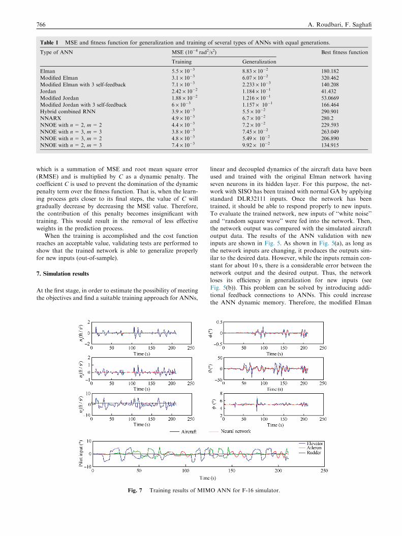
Table 1 MSE and fitness function for generalization and training of several types of ANNs with equal generations.

Type of ANN MSE (10�4 rad2/s2) Best fitness function

Training Generalization

Elman 5.5 · 10�3 8.83 · 10�2 180.182

Modified Elman 3.1 · 10�3 6.07 · 10�2 320.462

Modified Elman with 3 self-feedback 7.1 · 10�3 2.233 · 10�3 140.208

Jordan 2.42 · 10�2 1.184 · 10�1 41.432

Modified Jordan 1.88 · 10�2 1.216 · 10�1 53.0669

Modified Jordan with 3 self-feedback 6 · 10�3 1.157 · 10�1 166.464

Hybrid combined RNN 3.9 · 10�3 5.5 · 10�2 290.901

NNARX 4.9 · 10�3 6.7 · 10�2 280.2

NNOE with n = 2, m= 2 4.4 · 10�3 7.2 · 10�2 229.593

NNOE with n = 3, m= 3 3.8 · 10�3 7.45 · 10�2 263.049

NNOE with n = 3, m= 2 4.8 · 10�3 5.49 · 10�2 206.890

NNOE with n = 2, m= 3 7.4 · 10�3 9.92 · 10�2 134.915


which is a summation of MSE and root mean square error(RMSE) and is multiplied by C as a dynamic penalty. Thecoefficient C is used to prevent the domination of the dynamic

penalty term over the fitness function. That is, when the learn-ing process gets closer to its final steps, the value of C willgradually decrease by decreasing the MSE value. Therefore,

the contribution of this penalty becomes insignificant withtraining. This would result in the removal of less effectiveweights in the prediction process.

When the training is accomplished and the cost functionreaches an acceptable value, validating tests are performed toshow that the trained network is able to generalize properlyfor new inputs (out-of-sample).

7. Simulation results

At the first stage, in order to estimate the possibility of meetingthe objectives and find a suitable training approach for ANNs,

Fig. 7 Training results of MIM

linear and decoupled dynamics of the aircraft data have beenused and trained with the original Elman network havingseven neurons in its hidden layer. For this purpose, the net-

work with SISO has been trained with normal GA by applyingstandard DLR32111 inputs. Once the network has beentrained, it should be able to respond properly to new inputs.

To evaluate the trained network, new inputs of ‘‘white noise’’and ‘‘random square wave’’ were fed into the network. Then,the network output was compared with the simulated aircraft

output data. The results of the ANN validation with newinputs are shown in Fig. 5. As shown in Fig. 5(a), as long asthe network inputs are changing, it produces the outputs sim-ilar to the desired data. However, while the inputs remain con-

stant for about 10 s, there is a considerable error between thenetwork output and the desired output. Thus, the networkloses its efficiency in generalization for new inputs (see

Fig. 5(b)). This problem can be solved by introducing addi-tional feedback connections to ANNs. This could increasethe ANN dynamic memory. Therefore, the modified Elman

O ANN for F-16 simulator.


and hybrid combined recurrent networks (the innovated struc-ture) can be applied for better modeling and identification.

In Fig. 6, two types of networks, with and without addi-

tional self-feedbacks, are compared. This comparison indicatesthat, after adding suitable numbers of self-feedbacks to theANN neurons, the generalization abilities have been notably

improved. This makes the ANN model capable of predictingthe aircraft dynamics more accurately.

Table 1 shows the comparison between MSE and the fitness

function for the generalization and training data of severaltypes of ANNs with an equal number of generations. Thistable, in turn, shows the speed of training and generalizationabilities in ANNs. As shown in this table, compared to other

networks, the hybrid combined recurrent network has betterperformances in training and generalization.

Table 2 shows the comparison between the MSEs of the

hybrid combined RNN, which has been trained with normalGA (named as ‘‘normal ANN’’) and NNSOA (named as‘‘optimized ANN’’). The network has been trained well with

both methods, but the latter has a better performance andfewer errors in validating the out-of-sample inputs. Accordingto this table, the optimized ANN has caused the generalization

for the out-of-sample data to be improved significantly and thenumber of connections to be decreased by approximately 40%.It can also be concluded that, by using NNSOA in ANN train-ing, both feedback and feedforward connections may be recog-

nized as unnecessary weights and can be removed.After making sure about the better performance of the

hybrid combined recurrent network compared to other net-

works, this network has been chosen for training and validat-ing the aircraft coupled nonlinear dynamics.

For the purpose of modeling, an ANN with three inputs

including dE, dA, dR and six outputs including p; q; r; _u; _v; _wcan be used which is called multi-input multi-output (MIMO).If an MIMO structure is used, the input will be a matrix of

3 · nd, the desired output will be a matrix of 6 · nd, and the fit-ness criterion in the network will be as follows:

Fitness ¼ 1

KpMSEpþ; � � � ; þK _vMSE _v þ K _wMSE _w

ð36Þ

In this approach, the problem of choosing coefficients(Ki; i ¼ p; q; r; _u; _v; _wÞ will emerge. These coefficients shouldbe chosen in order to have appropriate results for all of the

six outputs. These coefficients should be able to neutralizethe differences between three rotational and three transitionalchannels in aircraft states, and also the average differences

between various channels by normalization. On this account,training was carried out for an ANN with three inputs, six out-puts, and seven neurons in the hidden layer. However, afterproducing over 100000 generations by using the GA, the

Table 2 MSE of ANNs for different inputs through two types

of training algorithms.

Type of input MSE (10�4 rad2/s2)

Normal GA NNSOA

3211 input (training) 1 · 10�5 1 · 10�5

Square wave input (validating) 4.163 · 10�4 2.318 · 10�4

Random input (validating) 1.588 · 10�3 1.752 · 10�4

Chirp signal (validating) 1.764 · 10�3 5.875 · 10�4

results, shown in Fig. 7, were not satisfactory. Therefore, inorder to have a better network performance in aircraft model-ing, six networks with three inputs and one output can be used

which is called multi-input single-output (MISO). By using sixMISO networks (Fig. 8), i.e., a separate network for everystate of the aircraft, the normalization problem will be obvi-

ated. In this structure, each network input vector is a matrixof 3 · nd, and the output vector is a matrix of 6 · nd. There-fore, in order to model and identify the aircraft dynamics

and have a better network generalization, six MISO networkswere used.

Fig. 9(a) shows the training results for the aircraft stateswhose data have been generated by the simulator. This figure

indicates that the proposed network is able to learn thedynamic behavior of the F-16 aircraft for in-sample (training)data. Fig. 9(b) shows the validation results of the ANN for

out-of-sample inputs, with which the aircraft performs variousmaneuvers (climb, descent, and turn). As it is clear, the ANNhas learned the aircraft dynamic behavior well and is able to

simulate and predict the aircraft flight dynamics for eachmaneuver.

Figs. 10 and 11(a) show the training results of actual flight

tests using the hybrid combined recurrent network at a specificMach and altitude with a multi-step input similar to 3211input. Fig. 11(b) shows the results of generalization with theout-of-sample data. The results confirm that, if the aircraft

remains in its initial trim conditions (around a given equilib-rium point), the ANN learns the aircraft’s actual behaviorand has acceptable generalization for the out-of-sample data.

Tables 3 and 4 present the MSE of the modified Elman net-work’s training and validation based on the simulated andexperimental data.

After training, the network has learned the coupling effectof aircraft control inputs on different parameters. Forinstance, the insignificant effect of the elevator on p, r, and_v; the aileron effect on r, _u, and _w. Figs. 12 and 13 presentthe results of these effects.

As mentioned previously, in addition to the pilot controlinputs, the flying vehicles dynamics depends on flight condi-

tions (Mach and altitude). Therefore, it cannot be expectedthat an ANN trained at a specific Mach and altitude can pro-duce acceptable results at other Mach and altitudes. The error

caused by the Mach-altitude effect on the trained ANN isshown in Fig. 14. In this figure, the ANN’s forward accelera-tion response (ANN output) is compared with the real data

generated by the conventional flight simulator at differentMach and altitudes. As shown in this figure, Mach and altitudehave a considerable effect on the aircraft dynamics and on thenetwork output accuracy, and only at a specific domain of

Mach (about 0.2) and altitude (about 5000 ft), it is more likelyto be sure of the network accuracy. The network trained at a

Fig. 8 MISO of ANNs model.

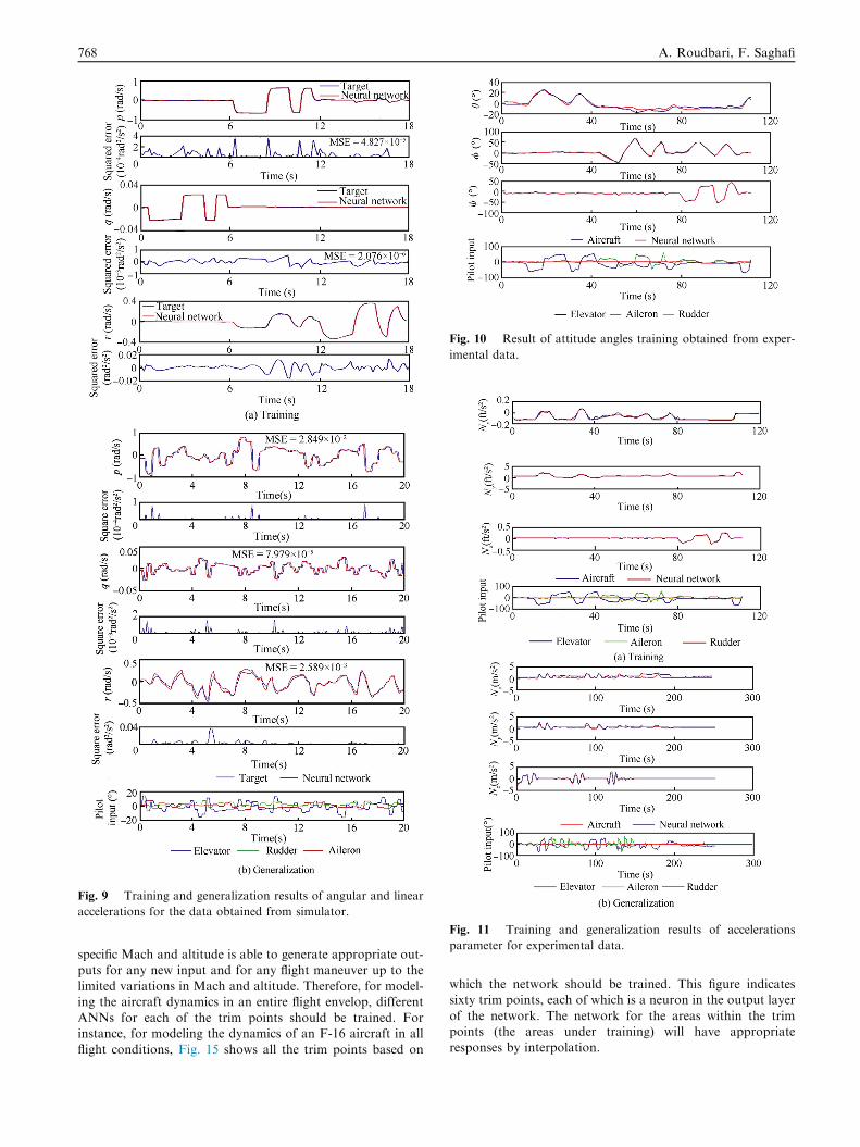
Fig. 9 Training and generalization results of angular and linear

accelerations for the data obtained from simulator.

Fig. 10 Result of attitude angles training obtained from exper-

imental data.

Fig. 11 Training and generalization results of accelerations

parameter for experimental data.


specific Mach and altitude is able to generate appropriate out-puts for any new input and for any flight maneuver up to the

limited variations in Mach and altitude. Therefore, for model-ing the aircraft dynamics in an entire flight envelop, differentANNs for each of the trim points should be trained. Forinstance, for modeling the dynamics of an F-16 aircraft in all

flight conditions, Fig. 15 shows all the trim points based on

which the network should be trained. This figure indicatessixty trim points, each of which is a neuron in the output layer

of the network. The network for the areas within the trimpoints (the areas under training) will have appropriateresponses by interpolation.

Table 3 MSE of training and validating modified Elman

network for F-16 data simulator.

State Training MSE Validating MSE

p 0.0482 0.0094

q 0.00002 0.00004

r 0.0001 0.31 · 10�3

_u 0.287 7.57

_v 1.14 14.36

_w 0.343 8.26

Table 4 MSE of training and validating modified Elman

network for experimental flight data.

State Training MSE Validating MSE

h 0.0026 0.0219

w 0.00011 0.006

/ 0.0013 0.1227

Nx 0.0123 0.4339

Ny 0.0089 0.1192

Nz 0.001 0.0047

Fig. 12 Results of validation for coupling effect of elevator on p,

r, and _v.

Fig. 13 Results of validation for coupling effect of aileron on r,

_u, and _w.

Fig. 14 Effects of Mach and altitude changes on network

outputs.

Fig. 15 Operational points and areas under training.



8. Conclusions

In this paper, by proposing a new approach for ANNs andsuitable training, it is shown that a highly maneuverable fighter

aircraft with nonlinear dynamics can be identified and pre-dicted through ANNs. It is additionally shown that ANNscan generalize new inputs in a satisfactory way without requir-

ing any error signals from the main system. On the whole, theresults produced and the observations made in this paper are:

(1) ANNs have been found to have enough potential for

identification of aircraft dynamics. The proposedmethod has the advantage of having a short computa-tion time and can estimate an acceptable model based

on flight tests. Therefore, the aircraft dynamics can bemodeled without requiring any aerodynamic models oraircraft dynamics derivatives and priori knowledge

about the aircraft dynamics model.(2) The generalizability of an ANN will improve if the ANN

is modified by introducing additional self-feedback

connections.(3) It has been shown that the proposed networks can be

trained successfully using NNSOA and a parsimoniousnetwork with enhanced generalizability can be obtained.

(4) In comparison with other networks, the hybrid com-bined recurrent network has demonstrated to have bet-ter performances with regard to training speed and

generalization.(5) After training, the ANN has learned the effects of cou-

pling among the aircraft’s control inputs.

Therefore, it can be concluded that ANNs can be applied indeveloping flight simulators for all types of aircraft and be

acceptable for aircraft modeling and identification based onknown flight tests data.

References

1. Stevens BL. Aircraft control and simulation. New York: John

Wiley and Sons Inc.; 1992.

2. Zipfed PH. Modeling and simulation of aerospace vehicle dynam-

ics. Reston: AIAA Inc.; 2000.

3. Tischler MB, Remple RK. Aircraft and rotorcraft system identi-

fication: engineering methods with flight test examples. Res-

ton: AIAA Inc.; 2006.

4. Ljung L. System identification theory for the user. 2nd ed. 1999.

5. Nelles O. Nonlinear system identification––from classical

approaches to neural networks and fuzzy models. New York:

Springer; 2001.

6. Klein V, Morelli EA. Aircraft system identification: theory and

practice. AIAA Inc.: Reston; 2006.

7. Tischler MB, Leung JGM, Dugan DC. Frequency-domain iden-

tification of XV-15 tilt-rotor aircraft dynamics in hovering flight.

AIAA 2nd flight testing conference; Las Vegas, Nevada. 1983.

8. Pintelon R, Schoukens J. System identification: a frequency domain

approach. 1st ed. New York: Wiley-IEEE Press; 2001.

9. Wang LX. Design and analysis of fuzzy identifiers of nonlinear

dynamic systems. IEEE Trans Automat Control 1995;40(1):11–23.

10. Qianqian R, Yi F. Flight dynamics identification of a helicopter in

hovering based on flight data. IEEE international conference on

artificial intelligence and computational intelligence; 2010.

11. Raptis IA, Valavanis KP, Kandel A, Moreno WA. System

identification for a miniature helicopter at hover using fuzzy

models. J Intell Robot Syst 2009;56(3):345–62.

12. van Overschee P, de Moor B. Subspace identification for linear

systems: theory, implementation, applications. Dordrecht: Kluwer

Academic Publishers; 1996.

13. Beaulieu MN, de JesusMota S, Botez RM. Identification of

structural surfaces’ positions on an F/A-18 using the subspace

identification method from flight flutter tests. Proc Inst Mech Eng,

Part G: J Aerosp Eng 2007;221(5):719–31.

14. Chen S, Billings SA, Grant PM. Non-linear system identification

using neural networks. Int J Control 1990;51(6):1191–214.

15. Boely N, Botez RM. New approach for the identification and

validation of a nonlinear F/A-18 model by use of neural networks.

IEEE Trans Neural Netw 2010;21(11):1759–65.

16. Boely N, Botez RM, Kouba G. Identification of a non-linear F/A-

18 model by the use of fuzzy logic and neural network methods.

Proc Inst Mech Eng G J Aerosp Eng 2011;225(5):559–74.

17. Samal MK, Anavatti S, Garratt M. Neural network based system

identification for autonomous flight of an eagle helicopter.

Proceedings of the 17th world congress the international federation

of automatic control (IFAC); 2008 Jul. 6–11, Seoul, Korea; 2008.

p. 7421–6.

18. Heimes F, Zalesski G, Walker Land Jr, Oshima M. Traditional

and evolved dynamic neural networks for aircraft simulation.

IEEE international conference on systems, man, and cybernetics;

1997 Oct. 12–15; 1997. p. 1995–2000.

19. Saghafi F, Heravi BM. Identification of aircraft dynamics using

neural network simultaneous optimization algorithm. Proceedings

of the European modeling and simulation conference (ESM 2005);

2005. p. 1–7.

20. Valmorbida G, Wen-Chi LU, Mora-Camino F. A neural

approach for fast simulation of flight mechanics. Proceeding of

the 38th Annual Simulation Symposium (ANSS’05); 2005 Apr. 4–6;

2005. p. 168–72.

21. Kamalasadan S, Ghandakly AA. A neural network parallel

adaptive controller for fighter aircraft pitch-rate tracking. IEEE

Trans Instrum Meas 2011;60(1):258–67.

22. Savran A, Tasaltin R, Becerikli Y. Intelligent adaptive nonlinear

flight control for a high performance aircraft with neural

networks. ISA Trans 2006;45(2):225–47.

23. Putro IE, Budiyono A, Yoon KJ, Kim DH. Modeling of

unmanned small scale rotorcraft based on neural network iden-

tification. Proceedings of the IEEE international conference on

robotics and biomimetics; 2009 Feb. 22–24; 2009.

p. 1938–43.

24. Sjoberg J, Zhang QH, Ljung L, Benveniste A, Delyon B,

Glorennec PY, et al. Nonlinear black-box modeling in system

identification: a unified overview. Automatica

1995;31(12):1691–724.

25. Witters M, Swevers J. Black-box identification of a continuously

variable semi-active damper. Proceedings of the IEEE multi

conference on systems and control; 2008 Sep. 3–5; 2008. p. 19–24.

26. Leontaritis IJ, Billings SA. Input–output parametric models for

non-linear systems Part I: deterministic non-linear systems. Int J

Control 1985;41(2):303–28.

27. Elman JL. Finding structure in time, state vectors were not zeroed

between words. Cogn Sci 1990;14:179–211.

28. Jordan MI. Serial order: a parallel distributed processing

approach. Report No.: ED276754.

29. Sexton RS, Dorsey RE. Simultaneous optimization of neural

network function and architecture algorithm. Decis Support Syst

2004;36(3):283–96.

30. Roskam J. Airplane flight dynamics and automatic flight controls.

1st ed. Ottawa: Roskam Aviation and Engineering Corporation;

1979.

http://refhub.elsevier.com/S1000-9361(14)00049-1/h0005

























































31. Plaetschke E, Mulder JA, Breeman JH. Flight test results of five

input signals for aircraft parameter estimation. Proceedings of the

6th IFAC symposium on identification and system parameter

estimation; 1982, Jan. 7–11; 1982. p. 1149–54.

32. Waibel A, Hanazawa T, Hinton G, Shikano K, Lang KJ.

Phoneme recognition using time-delay neural networks. IEEE

Trans Acoust Speech Signal Process 1989;37(3):328–39.

33. Pham DT, Karaboga D. Training Elman and Jordan networks for

system identification using genetic algorithms. Artif Intell Eng

1999;13(2):107–17.

34. Sexton RS, Gupta JND. Comparative evaluation of genetic

algorithm and backpropagation for training neural networks. Inf

Sci 2000;129(1–4):45–59.

35. Schaffer JD, Whitley D, Eshelman LJ. Combinations of genetic

algorithms and neural networks: A survey of the state of the art.

International workshop on combinations of genetic algorithms and

neural networks; 1992, Jun. 6; 1992. p. 1–37.

Alireza Roudbari is a Ph.D. student at Sharif University of Technol-

ogy, where he received his M.S. degree in 2005. His area of research

interest includes system identification, simulation and modeling, neural

network, fuzzy systems, and optimization.

Fariborz Saghafi is an associate professor of Flight Dynamics at Sharif

University of Technology. His main research interests consist of

intelligent identification of flying vehicles.










Documents

Intelligent modeling and identification of aircraft