An Algorithm for Parameters Identification of an Aircraft

1. Introduction

Development of efficient parameter identification methods for the model of a dynamic systembased on real-time measurements of some components of its state vector should be takenas one of the most important problems of applied statistics and computational mathematics.Calculating the motion of the system given the initial conditions and its mathematical model isconventionally called the direct problem of dynamics. Then, the inverse problem of dynamicswould be the problem of identifying the system model parameters based on measurementsof certain components of the state vector provided that the general structural scheme ofthe model is known from physical considerations. Such an inverse problem correspondsto identification problem for the dynamic system representing an aircraft. In this case, thegeneral structural scheme of the model (motion equations) follows from the fundamental lawsof aerodynamics.

In many cases, modern computational methods and wind tunnel experiments can providesufficient data on nominal parameters of the mathematical model - nominal aerodynamiccharacteristics of the aircraft. Nevertheless, there exist problems [1] that require correctingnominal parameters based on measurements taken in real flights. These imply

(1) verifying and interpreting theoretical predictions and results of wind tunnel experiments(flight data can also be used to improve ground prediction methods),

(2) obtaining more exact and complete mathematical models of the aircraft dynamics to beapplied in designing stability enhancement methods and flight control systems,

(3) designing flight simulators that require more accurate dynamic aircraft profile in all flightmodes (many motions of aircrafts and flight conditions can be neither reconstructed in thewind tunnel nor calculated analytically up to sufficient accuracy or efficiency),

(4) extending the range of flight modes for new aircrafts, which can include quantitativedetermination of stability and impact of control when the configuration is changed or whenspecial flight conditions are realized,

(5) testing whether the aircraft specification is compliant.

*This work has been supported by the Russian Foundation for Basic Research.

An Algorithm for Parameters Identification of an Aircraft’s Dynamics*

I. A. Boguslavsky State Institute of Aviation Systems, Moskow Physical Technical Institute

Russia

6

www.intechopen.com

2 Will-be-set-by-IN-TECH

Furthermore, dimensionless numbers at the nodes of one-or two-dimensional tables found inwind tunnel experiments serve as nominal values in the aerodynamic parameter identificationproblem of the aircraft. This causes the vector that corrects these parameters determinedby the algorithm processing digital data flows received from the aircraft sensors to have asignificant dimension of the order about several tens or hundreds.

It is worth noting that the USA (NASA) is doing extensive work on theoretical and practicalaircraft identification by test flights. In 2006 alone, in addition to many journal publications,American Institute of Aeronatics and Astronatics (AIAA) published three fundamentalmonographs [1-3] on the subject. An implementation of multiple NASA recommendedalgorithms for identification problems, SIDPAS (Systems Identification Programs for Aircraft)software package written in MATLAB M-files language is available on the Internet as anappendix to [1]. Various existing identification methods published in monographs on statisticsand computational mathematics are widely reviewed in [1].

For the most general identification method, one should take the known nonlinear least squaresmethod [4] that forms the sum of errors squared - differences between the real measurementsand their calculated analogues obtained by numerical integration of motion equations of thesystem for some realization of the vector of unknown parameters.

Successful identification yields the vector of parameters that delivers the global minimum tothe above mentioned sum of errors squared. Still, this criterion is statistically valid only forlinear identification problems, in which measurements are linear with respect to the unknownvector of parameters.

Implementing the nonlinear least squares method to correct nominal parameters of theaircraft based on its test flight data involves computational challenges. These arise when thedimension of the correction vector is big and the sum of errors squared as the function of thecorrection vector has multiple relative minimums or when variations of the Newton’s methodare applied, with the sequence of local linearizations performed to find stationary points ofthis function. In [1], the regression method supported by lesq.m, smoo.m, derive.m, and xstep.mfiles in SIDPAS is recommended for practical applications.

Suppose the motion equations of the system and the sequence of measurements have the form

dx/dt = f (x, ϑ + η, u), ...(0.1)

yk = Hk(x(tk)) + ξk, ...(0.2)

where x(tk) is the n × 1-dimensional vector of the system states at the current instant t andat the given instants tk, k = 1, ..., N, ϑ is the r × 1-vector of nominal (known) parametersof the system, η is the vector of unknown parameters that serves as the correction vectorfor the nominal vector ϑ after the results of measurements are stochastically processed, uis the control vector of the system, f (...) is the given vector-function, yk is the sequence ofvectors-results of measurements, Hk(...) is the given vector function, and ξk, k = 1, ..., N is thesequence of random vectors-errors of measurements with the given random generator for themathematical simulation.

We can state the identification problem for the vector η as follows. Find the estimate as thefunction of the vector YN formed of the results of all measurements y1, ...yN.

120 Recent Advances in Aircraft Technology

www.intechopen.com

The Inverse Problem - an Algorithm for Parameters Identification of an Aircraft’s Dynamics 3

The regression method given in [1] solves this problem under the following limitations

(1) all components of the state vector can be measured : yk = x(tk) + ξk,

(2) at the measurement instants tk, the algorithm constructs the estimate of the vector ofderivatives dx/dt,

(3) the vector function f (x, ϑ + η, u) linearly depends on the vector η.

These fundamental limitations of the regression method duplicate features of theidentification algorithm from [5]. The substantial drawback of the algorithm [5] and thealgorithm of the regression method is that they do not allow using the mathematical model toanalyze theoretically (without applying the Monte-Carlo method) observability conditions ofcomponents of the vector of parameters to be identified for the preliminary given control lawfor the test flight of the aircraft and information on random errors of its sensors. Note that thisis the drawback of all known numerical methods that solve nonlinear identification problems.

Relations (0.1) and (0.2) show that when conditions (1)-(3) are met and N is sufficiently big,the estimation vector satisfies the overdetermind system of linear algebraic equations, withmethods to solve it being well known. The given conditions seem to be rather rigid andmay be hard-to-implement. For instance, it is arguable whether one can construct the vectorof derivatives dx/dt sufficiently accurately given the real turbulent atmosphere conditions,which imply that the outputs of the angle of attack and sideslip sensors inevitably includerandom and unpredictable frequency components.

All this justifies the development of new identification algorithms that can be applied todynamic systems of a rather general class and do not possess drawbacks of NASA algorithms.The proposed multipolynomial approximation algorithm (MPA algorithm) serves as such anew identification algorithm.

2. Statement of the problem and basic scheme of the proposed identification

algorithm

The general scheme for identifying aerodynamic characteristics of the aircraft by the test flightdata is as follows [1]. Motion equations of the aircraft (0.1) and system (0.2) of measurementsof motion characteristics of the aircraft are given. The vector ϑ is the vector of nominalaerodynamic parameters determined in the wind tunnel experiment. Calculated by the resultsof real (test) flight, the vector η is used to correct the vector ϑ.

When the aircraft flies, its computer fixes the digital array of initial conditions and timefunctions, viz. current control surface angles and measurements of some motion parametersof the aircraft (some components of the vector x(t) of the state of the aircraft) received fromits sensors. Note that selecting the criterion for optimal or, at least, rational mode to controlthe test flight is a separate problem and lies beyond our further consideration. The currentmotion characteristics measured as the time function such as angles of attack and sideslip andcomponents of the vector of angular velocity and g-load obtained by the inertial system ofthe aircraft are registered for real (not known for sure) aerodynamic parameters of the aircraft(parameters ϑ + η) and can be called measured characteristics of the perturbed motion.

121An Algorithm for Parameters Identification of an Aircraft’s Dynamics

www.intechopen.com


Once the flight under the mentioned (given) initial conditions and time functions (controlsurface angles) is completed, nominal motion equations (equations of form (1) for η = 0)are integrated numerically for the nominal aerodynamic parameters of the aircraft. For thecalculated characteristics of the nominal motion of the aircraft one should take the obtaineddata - components of the state vector of the aircraft as the function of discrete time. Differencesbetween measurable characteristics of the perturbed motion and calculated characteristicsof the nominal motion serve as carriers of data on the unknown vector η that shows thedifference between real and nominal aerodynamic parameters.

The input of the MPA identification algorithm receives the vector of initial conditions andcontrol surface angles as functions of time and arrays of characteristics of nominal andperturbed motions.

The output of the algorithm is η(YN) , which is the correction vector for nominal aerodynamicparameters.

The identification algorithm is efficient if the motion equations integrated numerically withthe corrected aerodynamic parameters yield such motion characteristics ϑ + η(YN) (correctedcharacteristics, in what follows) that are close to real (measurable) characteristics.

In this work, we consider the technology of applying the Bayes MPA algorithm [6, 7] tosolve identification problems on the example of the aircraft, for which nominal aerodynamicparameters of the pitching motion are the nominal parameters of one of an "pseudo" F-16aircraft.

We replace real flights by mathematical simulation, with characteristics of the perturbedmotion obtained by integrating the motion equations of the aircraft numerically. In theseequations, nominal aerodynamic parameters at the nodes of the corresponding tables arechanged to random values that do not exceed in modulus the given 25 ÷ 50 percents ofnominal values at these nodes.

Fundamentally, the MPA algorithm assumes that the vector of unknown parameters η israndom on the set of possible flights. We assume that the a priori statistical-generator forcomputer generated random vectors η and ξk is given. This generator makes the algorithmestimating components of the vector η (the identification algorithm) Bayesian. Further, forparticular calculations, we assume that random components of the mentioned vectors aredistributed uniformly and can be called by the standard Random program in Turbo Pascal.

The MPA algorithm provides the approximation method we implement with themultidimensional power series of the vector E(η|YN) of the conditional mathematicalexpectation of the vector η if the vector of measurements YN is fixed and a priori statisticaldata on random vectors η and ξk are given.

The vector E(η|YN) is known to be optimal, in root-mean-square sense, estimate of the randomvector η.

We describe the steps of operation of the MPA algorithm when it identifies the vector η[6, 7].

Step 1. Suppose d is a given positive integer number and the set of integer numbers a1, ..., aN

consists of all nonnegative solutions of the integer inequality a1 + ... + aN ≤ d, the number ofwhich we denote by m(d, N). The value m(d, N) is given by the recurrent formula proved by


www.intechopen.com


induction.m(d, N) = m(d − 1, N) + (N + d − 1) · · · N/d!, m(1, N) = N.

We obtain the vector WN(d) of dimension m(d, N) × 1, the components w1, ..., wm(d, N) ofwhich are all possible values ya1

1 ...yan

N of the form that represent the powers of measurablevalues.

Then, we construct the base vector V(d, N) of dimension (r + m(d, N)) × 1, V(d, N) =‖ηWN(d)‖.

Step 2. We use a known statistical generator of random vectors η and ξk to solve repeatedlythe Cauchy problem for Eq.(1) for given initial conditions x(0), a control law u(t) and variousrealizations of random vectors η and xik.

We apply the Monte-Carlo method to find the prior first and second statistical moments ofthe vector V(d, N), i.e., the mathematical expectation V(d, N), and the covariance matrixCV(d, N) = E((V(d, N)− V(d, N))(V(d, N)− V(d, N))T) .

Implementation of step 2 is a learning process for the algorithm, adjusting it to solve theparticular problem described by Eqs. (1) and (2).

Step 3. For given d and N and a fixed vector YN , we assign the vector η(WN(d)) to be thesolution to the estimation problem. This vector gives an approximate estimate of the vectorE(η|YN) that is optimal in the root-mean-square sense on the set of vector linear combinationsof components of the vector WN1

(d)

η(WN(d)) = ∑a1+...+aN≤d

λ(a1, ..., aN)ya1

1 · · · yaN

N . (1.1)

The vector V(d, N) and the matrix CV(d, N) are the initial conditions for the process ofrecurrent calculations that realizes the principle of observation decomposition [6] and consistsof m(d, N) steps. Once the final step is performed, we obtain vector coefficients λ(a1, ..., aN)for (1.1). Moreover, we determine the matrix C(d, N), which is the covariance matrix of theestimation errors for the vector E(ηN |YN) of conditional mathematical expectation estimatedby the vector η(WN(d)).

Calculating the elements of the matrix C(d, N), we have the method of preliminary (prior tothe actual flight) analysis of observability of identified parameters for the given control law,structure of measurements and their expected random errors. Recurrent calculations do notrequire matrix inversion and indicate the situations when the next component of the vectorWN(d) is close to linear combination of its previous components. To implement the recursion,we process the components of the vector WN(d) one after another. However, the adjustment ofthe algorithm performed by applying the Monte-Carlo method to find the vector V(d, N) andthe matrix CV(d, N) takes into account a priori ideas on stochastic structure of componentsof the whole set of possible vectors WN(d) that can appear in any realizations of the randomvectors η and ξk allowed by the a priori conditions.

This adjustment is the price we have to pay if we want the MPA algorithm to solvenonlinear identification problems efficiently. This is what makes the MPA algorithm differfundamentally from, for instance, the standard Kalman filter designed to solve linear


www.intechopen.com


identification problems only or from multiple variations of algorithms resulted from attemptsto extend the Kalman filter to nonlinear filtration problems.

In [6], a multidimensional analogue of the K. Weierstrass theorem (the corollary of the M.Stone theorem [9]) is used to prove that when the integer d is increases then the error estimatesof the vector E(η|YN) the vector |η(WN(d))−E(η|YN)| tend to zero uniformly on some region.Formulas of the recurrent algorithm are given and justified in [6, 7] and in the Appendix.

This scheme for the MPA algorithm operation shows that it can be applied to identifyparameters of almost any dynamic system provided that the structures of the motionequations and measurements of form (0.1) and (0.2) and prior statistical generators of randomunknown parameters and errors of measurements are given. The MPA algorithm is devoid ofthe above listed limitations and drawbacks, which gives it substantial advantages over NASAidentification algorithms. Apart from errors of computations, the algorithm does not addany other errors (such as errors due to linearization of nonlinear functions) into the identifiedparameters. Therefore, one should expect that the priori spread of identifiable parameters tobe always greater than the posterior spread. This is why we can use iterations.

Let us compare the sequential steps of the standard discrete Kalman filter and the MPAalgorithm.

(1) The Kalman filter identifies the vector η, which can be represented by part of componentsof the state vector of the linear dynamic system for the observations that linearly depend onstate vectors. The a priori data are the first and second moments of components of randominitial state vectors, uncorrelated random vectors of perturbations and observation errors.We need these data for sequential (recurrent) construction of the estimation vector that isroot-mean-square optimal. Usually assigned, a priori data can be also determined by theMonte-Carlo method if the complex mechanism of their appearance is given.

(2) To find an asymptotic solution to the nonlinear identification problem, the MPA algorithm,unlike the Kalman filter, requires a priori statistical data on both the initial and allhypothesized future state vectors of the dynamic system and observations. These a prioridata are represented by the first and second statistical moments for the random vector V(d,N): the vector V(d, N)) and the matrix CV(d, N). These moments are calculated using theMonte-Carlo method. However, there are cases when they can be obtained by numericalmultidimensional region integration.

(1.1) Once conditions from (1) are met, the Kalman filter constructs the recurrent process, atevery step of which the current estimation vector optimal in the root-mean-square sense andthe covariance matrix of errors of the estimate are calculated.

(2.1) Based on (2), the MPA algorithm implements the recurrent computational process thatdo not require matrix inversion. At each step of the process, we construct

i. the current estimation vector η(WN(d)) linear with respect to components of the vectorWN(d) and optimal in the root-mean-square sense on the set of linear combinations ofcomponents of this vector; moreover, the uniform convergence η(WN(d)) → E(η|YN), d → ∞.is attained on some region,


www.intechopen.com


ii. the current covariance matrix of estimation errors (we emphasize that known numericalmethods of constructing approximations of the vector of nonlinear estimates cannot calculatecurrent covariance matrices of estimation errors).

Implementation of items 2 and 2.1 makes the MPA algorithm more efficient than any knownlinear identification algorithm since it

i. does not involve linearization,

ii. does not apply variants of the Newton method to solve systems of nonlinear algebraicequations,

iii. forms the estimation vector that tends uniformly to the vector of conditional mathematicalexpectation for the growing integer d,

iiii. obtains the covariance matrix of estimation errors.

It is worth emphasizing that in this work we just develop the fundamental ground ofcomputational technique for solving the complex problem of aircraft parameter identification.

3. Testing the MPA algorithm: Problem reconstruction (identification of

parameters) for the attractor from units of an electrical chain

We consider the boundary inverse problem for the attractor whose equations are presented in[8 ]. The three parameters are the initial conditions: X1[0] = η1, X2[0] = η2, X3[0] = η3. Thesix parameters η3+i, i = 1, ..., 6 correspond to combinations of the inductance, the resistancesand the two capacitances of a circuit.

The equations of the mathematical model of the circuit take the following form [8]:

X1[k − 1] < −η3+6 : f = η3+5;

−η3+6 < X1[k − 1] < η3+6 : f = X1[k − 1](1 − X1[k − 1]2);

X1[k − 1] > η3+6 : f = −η3+5;

X1[k] = X1[k − 1] + δX2[k − 1];

X2[k] = X2[k − 1] + δ(−X1[k − 1]− η3+1X2[k − 1] + X3[k − 1]);

X3[k] = X3[k − 1] + δ(θ3+2(η3+3 f − X3[k − 1])− η3+4X2[k − 1]);

where X1[k] corresponds to a voltage, X2[k] to a current and X3[k] to another voltage.

We suppose that by i = 1, 2, 3ηi ∈ 1 + (εi − 0.5).

We also suppose [ 8] that

η3+1 ∈ 0.5(1 + (ε1 − 0.5)); η3+2 = 0.3(1 + (ε2 − 0.5)); η3+3 = 15(1 + (ε3 − 0.5));

η3+4 ∈ 1.5(1 + (ε4 − 0.5)); η3+5 = 0.5(1 + (ε5 − 0.5)); η3+6 = 1.2(1 + (ε6 − 0.5));

yk = X1(tk)) + ζk

δ = 0.01, k = 1, ..., N = 1200, z1 = ∑k=N/Tk=1 yk, z2 = ∑

k=2×N/Tk=1+N/T yk,...


www.intechopen.com


The algorithm uses approximations of parameters by means of linear combinations of theconstructed values zi(d = 1). Values z1, z2 - are the sums of values of flowing observations -serve as inputs of MPA algorithm

The relative errors of the boundary problem are

i 1 2 3

T = 24

Δi 0.025 0.264 0.272

T = 48

Δi 0.0007 −0.003 0.046

T = 120

Δi 0.00005 −0.00264 0.01687

T = 240

Δi 0.00001 −0.00049 0.02686

.

The relative errors of the inverse problem are

i 1 2 3 4 5 6

T = 24

Δ3+i −0.347 0.198 −0.250 0.097 0.095 0.136T = 48

Δ3+i −0.140 0.234 −0.222 0.104 0.143 0.133

T = 120

Δ3+i −0.169 0.205 −0.167 0.094 0.179 0.097

T = 240

Δ3+i −0.042 0.129 −0.031 −0.0001 0.151 0.146

.

The resulted tables show, that corresponding adjustment the MPA algorithm - a correspondingselection of value T allows to make small relative errors of an estimation of parameters of thenon-linear dynamic system.

4. Identification of aerodynamic coefficients of the pitching motion for an pseudo

f-16 aircraft

We illustrate efficiency of offered MPA algorithm on an example of identification of 48dimensionless aerodynamic coefficients for the aircraft of near F-16. The aircraft we shallconditionally name " pseudo F-16 ". The term "near" is justified by that, what is the coefficientsare taken from SIDPAS [1], but are perturbed by addition of some random numbers.

The tables resulted below, show, that errors of identification are small also modules of theirrelative values do not surpass several hundredth. The considered problem corresponds tominimization of object function of 48 variables, which it is made of the sum of squares ofdifferences of actual and computational angles of attack, g-load, pitch angles, observable withfrequency 10 hertz during 25 sec. flight of the aircraft maneuvering in a vertical plane.


www.intechopen.com


number αi CZ0(αi) Cm0 (αi) CZq

(αi) Cmq (αi)

1 0.7700 −0.1740 −8.8000 −7.21002 0.2410 −0.1450 −25.8000 −5.40003 −0.1000 −0.1210 −28.9000 −5.23004 −0.4160 −0.1270 −31.4000 −5.26005 −0.7310 −0.1290 −31.2000 −6.11006 −1.0530 −0.1020 −30.7000 −6.64007 −1.3660 −0.0970 −27.7000 −5.69008 −1.6460 −0.1130 −28.2000 −6.00009 −1.9170 −0.0870 −29.0000 −6.200010 −2.1200 −0.0840 −29.8000 −6.400011 −2.2480 −0.0690 −38.3000 −6.600012 −2.2290 −0.0060 −35.3000 −6.0000

Table 1. Nominal values of the functions CZ0(α), Cm0 (α), CZq

(α), Cmq (α)

4.1 Pitching motion equations

We use the rectangular coordinate system XYZ adopted in NASA. Then for the unperturbedatmosphere and conditions V = const, pitching motion equations have the form [1]:

dα/dt = ωY + (g/V)(NZ + cos(θ − α)),

dωY/dt = MY/JY ,

dθ/dt = ωY ,

NZ = CZ(α, δs)qS/G,

MY = Cm(α, δs)qSb,

where V=300 ft/sec,H=20000 ft, α is the angle of attack, NZ is the g-load, which is the vectorof aerodynamic forces projected onto the axis Z and divided by the weight of the aircraft,MY is the vector of the moment of aerodynamic forces projected onto the axis Y, ω is thevector of the angular velocity of the aircraft projected onto the axis Y,θ is the angle betweenthe the axis X and the horizontal plane, q is the value of the dynamic pressure, G is theweight, JY is the moment of inertia with respect to the axis Y, S is the area of the surfacegenerating aerodynamic forces, b is the mean aerodynamic of the wing, CZ(α, δ) and Cm(α, δ)are dimensionless coefficients of the aerodynamic force and moment,δs is the angle of thestabilator devlection measured in degrees.

Functions CZ(α, δs) and Cm(α, δs) are given by the relations [1],:

CZ(α, δs) = CZ0(α)− 0.19(δs/25) + CZq

(α)(b/(2V))ω,

Cm(α, δs) = Cm0 (α)δs + Cmq (α)(b/(2V))ω + 0.1CZ.

4.2 Parametric model aerodynamic forces and moments

Nominal values of 4 functions of the angle of attack CZ0(α), Cm0 (α), CZq

(α), Cmq (α) are given

with the argument step (55 − 1)/12 degree at 12 nodes (Table 1) in range −10 ≤ α ≤ 45 .

To determine values of functions between the nodes, we use linear interpolation. Havinganalyzed Table 1, we can see that functions CZ0

(αi), Cm0 (αi), CZq(αi), Cmq (αi) are essentially


www.intechopen.com


number αi Δ(CZ0(αi)) Δ(Cm0 (αi)) Δ(CZq

(αi)) Δ(Cmq (αi))

1 0.7700 −0.1740 −8.8000 −7.21002 −0.5290 0.0290 −17.0000 1.81003 −0.3410 0.0240 −3.1000 0.17004 −0.3160 −0.0060 −2.5000 −0.03005 −0.3150 −0.0020 0.2000 −0.85006 −0.3220 0.0270 0.5000 −0.53007 −0.3130 0.0050 3.0000 0.95008 −0.2800 −0.0160 −0.5000 −0.31009 −0.2710 0.0260 −0.8000 −0.200010 −0.2030 0.0030 −0.8000 −0.200011 −0.1280 0.0150 −8.5000 −0.200012 0.0190 0.0630 3.0000 0.6000

Table 2. Nominal values of increment Δ(CZ0(αi)), Δ(Cm0 (αi)), Δ(CZq

(αi)), Δ(Cmq (αi))

nonlinear. Table 2 confirms this visual impression. In it increments are presented 4 functionson each step of Table 1. Apparently, increments noticeably vary.

We study the identification problem for the perturbed analogues of the functionsCZ0

(α), Cm0 (α), CZq(α), Cmq (α). The number of nominal coefficients that determine these

functions is 12+12+12+12 = 48. Let us single out the problem which is the most complexfor the MPA algorithm, when the actual coefficients differs from the nominal coefficientsby the unknown bounded by the prior limits value ηi at each point of the table. Then,for accumulated results of measurements of parameters of the perturbed motion, the MPAalgorithm is to estimate 48 components of the vector of random estimates, - the vector ofdifferences between actual and nominal coefficients.

Suppose ϑi and Bi are the i-th components of the nominal and actual (perturbed) vectors ofaerodynamic coefficients , i = 1, ..., 48, i.e. the number of actual coefficients to be identified is48 in this case. We assume that the parametric model

Bi = ϑi + ηi.

holds. The vector η serves as the vector of perturbations of nominal data errors ofaerodynamic parameters, and identification yields the estimates of its components. We givethe structure of these components by the formula ηi = ϑiρiεi, 0 < ρi < 1,−1 < εi < 1.The positive number ρi gives the maximum value that, by identification conditions, can beattained by the ratio of the absolute values of the random value of perturbations ηi andnominal coefficients ϑi .

4.3 Transient processes of characteristics of nominal motions

We wish to identify-estimate - during one test flight the 48 unknown aerodynamic coefficientsfor 12 nodes-12 the set angles of attack αi, i = 1..., 12. For a testing maneuver thecharacteristics α(t), NZ(t), θ(t) of Transient Processes are carrier of information of the theidentified coefficients. Therefore during flight the aircraft should "visit" vicinities of anglesof attack −10 ≤ α ≤ 45


www.intechopen.com


number. obs. k δs(k) α(k) NZ(k) θ(k)1 −0.0200 3.6820 0.1021 0.01323 −0.0600 5.1462 −0.3525 0.13885 −0.1000 6.0119 −0.2956 0.16897 −0.1400 6.7707 −0.2493 0.03009 −0.1800 7.5061 −0.2085 −0.1851

11 −0.2200 8.2964 −0.1685 −0.394513 −0.2600 9.2186 −0.1253 −0.522715 −0.3000 10.2083 −0.6016 −0.511917 −0.3400 10.6145 −0.5691 −0.618719 −0.3800 10.8889 −0.5477 −0.889121 −0.4200 11.0977 −0.5334 −1.246123 −0.4600 11.2993 −0.5223 −1.625225 −0.5000 11.5494 −0.5114 −1.968827 −0.5400 11.9047 −0.4974 −2.222229 −0.5800 12.4277 −0.4774 −2.328631 −0.6200 13.1919 −0.4477 −2.224733 −0.6600 14.2870 −0.4043 −1.835235 −0.7000 15.4810 −0.8822 −1.148137 −0.7400 16.1493 −0.8343 −0.658239 −0.7800 16.6530 −0.7993 −0.382841 −0.8200 17.0629 −0.7728 −0.238243 −0.8600 17.4401 −0.7511 −0.155245 −0.9000 17.8400 −0.7310 −0.074747 −0.9400 18.3168 −0.7095 0.057149 −0.9800 18.9260 −0.6838 0.292651 −1.0200 19.7287 −0.6512 0.685553 −1.0600 20.1833 −1.1389 1.134355 −1.1000 20.1954 −1.1266 1.307557 −1.1400 19.9812 −1.1273 1.248659 −1.1800 19.9888 −1.1293 1.157261 −1.2200 19.9789 −1.1308 1.114663 −1.2600 20.0083 −1.1316 1.112965 −1.3000 20.0049 −1.1325 1.143767 −1.3400 20.0371 −1.1330 1.211369 −1.3800 20.0328 −1.1338 1.307371 −1.4200 20.0598 −1.1344 1.435973 −1.4600 20.0636 −1.1346 1.605375 −1.5000 20.0993 −1.1344 1.806977 −1.5400 20.1945 −1.1326 2.067179 −1.5800 20.3760 −1.1278 2.409681 −1.6200 20.6696 −1.1186 2.855883 −1.6600 21.1005 −1.1037 3.424785 −1.7000 21.6926 −1.0820 4.133187 −1.7400 22.4690 −1.0523 4.994889 −1.7800 23.4509 −1.0133 6.0212


www.intechopen.com


91 −1.8200 24.6576 −0.9641 7.220193 −1.8600 25.7086 −1.3912 8.610395 −1.9000 26.9187 −1.3506 10.291397 −1.9400 28.6178 −1.2942 12.408599 −1.9800 30.7696 −1.6768 15.0754

101 −2.0200 32.4354 −1.6031 17.5706103 −2.0600 33.8743 −1.5431 19.7731105 −2.1000 35.1432 −1.8357 21.7958107 −2.1400 35.7317 −1.8014 23.4808109 −2.1800 35.9655 −1.7815 24.7918111 −2.1800 35.9159 −1.7715 25.8128113 −2.1400 35.6010 −1.7680 26.5691115 −2.1000 34.9990 −1.7695 27.0436117 −2.0600 34.7166 −1.4423 27.4338119 −2.0200 34.4743 −1.4525 27.8824121 −1.9800 34.2309 −1.4610 28.3457123 −1.9400 33.9488 −1.4692 28.7851125 −1.9000 33.5921 −1.4785 29.1649127 −1.8600 33.1250 −1.4900 29.4506129 −1.8200 32.5103 −1.5050 29.6075131 −1.7800 31.7080 −1.5248 29.5992133 −1.7400 30.6740 −1.5505 29.3864135 −1.7000 29.6897 −1.1403 29.0369137 −1.6600 29.5906 −1.1751 29.2924139 −1.6200 30.0407 −1.6327 30.1792141 −1.5800 30.0324 −1.1643 30.9954143 −1.5400 30.0007 −1.1623 31.6784145 −1.5000 29.9971 −1.1623 32.3405147 −1.4600 29.9834 −1.6165 32.9999149 −1.4200 29.9916 −1.1620 33.6324151 −1.3800 29.9805 −1.1621 34.2532153 −1.3400 30.0190 −1.1626 34.8756155 −1.3000 29.9687 −1.6164 35.4719157 −1.2600 30.0181 −1.1623 36.0635159 −1.2200 29.9808 −1.1614 36.6311161 −1.1800 29.9772 −1.1614 37.1835163 −1.1400 29.9490 −1.6153 37.7184165 −1.1000 29.9574 −1.1606 38.2407167 −1.0600 29.9417 −1.6141 38.7453169 −1.0200 29.9178 −1.1614 39.1922171 −0.9800 29.8635 −1.1625 39.6161173 −0.9400 29.7346 −1.1650 39.9729175 −0.9000 29.4842 −1.1711 40.2178177 −0.8600 29.0596 −1.1829 40.3020179 −0.8200 28.3990 −1.2028 40.1699


www.intechopen.com


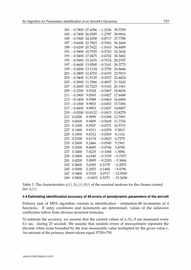
181 −0.7800 27.4286 −1.2336 39.7559183 −0.7400 26.0585 −1.2787 38.9816185 −0.7000 24.4358 −0.8717 37.7788187 −0.6600 22.7903 −0.9362 36.2669189 −0.6200 20.7622 −1.0163 34.4409191 −0.5800 18.7935 −0.5743 32.3636193 −0.5400 17.0475 −0.6702 30.3402195 −0.5000 15.1676 −0.7674 28.2787197 −0.4600 13.9500 −0.3141 26.3775199 −0.4200 13.1154 −0.3750 24.8646201 −0.3800 12.4703 −0.4193 23.5913203 −0.3400 11.9129 −0.4537 22.4424205 −0.3000 11.3566 −0.4837 21.3242207 −0.2600 10.7223 −0.5143 20.1561209 −0.2200 9.9324 −0.5497 18.8636211 −0.1800 9.8365 −0.0427 17.6449213 −0.1400 9.9588 −0.0463 16.6494215 −0.1000 9.9853 −0.0452 15.7456217 −0.0600 9.9853 −0.0437 14.8087219 −0.0200 10.0132 −0.0415 13.8278221 0.0200 9.9999 −0.0398 12.7981223 0.0600 9.9409 −0.5639 11.7156225 0.1000 9.9557 −0.0371 10.5715227 0.1400 9.9311 −0.0359 9.3815229 0.1800 9.8312 −0.0369 8.1116231 0.2200 9.6174 −0.0423 6.7279233 0.2600 9.2466 −0.0540 5.1941235 0.3000 8.6685 −0.0746 3.4700237 0.3400 7.8225 −0.1068 1.5084239 0.3800 6.6340 −0.1539 −0.7475241 0.4200 5.0095 −0.2203 −3.3684243 0.4600 3.6383 0.2178 −6.2070245 0.5000 2.2053 0.1484 −9.0796247 0.5400 0.5330 0.0717 −12.0920249 0.5800 −0.9453 0.5373 −15.2658

Table 3. The characteristics α(t), NZ(t), θ(t) of the nominal motions for the chosen controllaw δs(t).

4.4 Estimating identification accuracy of 48 errors of aerodynamic parameters of the aircraft

Primary task of MPA algorithm consists in identification - estimation-48 increments of 4functions. If entry conditions and increments are determined, values of the unknowncoefficients follow from obvious recurrent formulas.

To estimate the accuracy, we assume that the current values of α, NY , θ are measured every0.1 sec. during 25 seconds .We assume that random errors of measurement represent thediscrete white noise bounded by the true measurable value multiplied by the given value ǫ.An amount of the primary observations equal 3*250=750.


www.intechopen.com


number αi nom.koef. CZ0(αi) perturb.koef. CZ0

(αi) δ(CZ0(αi))

1 0.6512 0.6326 0.02854

2 0.0205 0.0260 −0.26410

3 −0.3778 −0.3646 0.03491

4 −0.7395 −0.7213 0.02456

5 −1.0610 −1.0657 −0.00443

6 −1.4038 −1.4016 0.00159

7 −1.7679 −1.7424 0.01444

8 −2.0582 −2.0453 0.00627

9 −2.2774 −2.3388 −0.02693

10 −2.4568 −2.5459 −0.03625

11 −2.5639 −2.6698 −0.04130

12 −2.5404 −2.6505 −0.04334

Table 4. The Relative errors of the identifications of CZ0(αi) by ρ = 0.25

number αi nom.koef. Cm0 (αi) perturb.koef. Cm0 (αi) δ(Cm0 (αi))

1 −0.2130 −0.2054 0.03582

2 −0.1816 −0.1783 0.01851

3 −0.1567 −0.1550 0.01061

4 −0.1618 −0.1611 0.00439

5 −0.1634 −0.1631 0.00209

6 −0.1427 −0.1388 0.02754

7 −0.1372 −0.1338 0.02439

8 −0.1495 −0.1502 −0.00467

9 −0.1175 −0.1220 −0.03771

10 −0.1139 −0.1190 −0.04484

11 −0.0957 −0.1043 −0.08937

12 −0.0399 −0.0394 0.01236

Table 5. The Relative errors of the identifications of Cm0 (αi) by ρ = 0.25

We compress primary observations for a smoothing the high-frequency errors and reductionof a dimension of matrixes covariance . The file of the primary observations is divided into12 groups and as an input of the algorithm of the identification the vector of the dimension12 × 1 serves. Components of this vector are the sums of elements of each of 12 groups.

To characterize the accuracy of identification of the random parameter ηi the degree ofperturbation of the aerodynamic coefficients ϑ , we determine the relative errors of estimation(ηi − ηi)/ηi for every component the identifiable functions . The relative errors designateδ(CZ0

(αi)), δ(Cm0 (αi)), δ(CZq(αi)), δ(Cmq (αi)), i = 1, ..., 12.

Apparently, relative errors of identification are small and do not surpass several hundredth atρ = 0.25


www.intechopen.com


number αi nom.koef. CZq(αi) perturb.koef. CZq

(αi) δ(CZq(αi))

1 −9.9636 −8.8984 0.106912 −25.2235 −26.1655 −0.037353 −28.4644 −29.2857 −0.028854 −31.4821 −31.8270 −0.010965 −31.3125 −31.6274 −0.010066 −30.8417 −31.1249 −0.009187 −27.5461 −28.0921 −0.019828 −28.1388 −28.6036 −0.016529 −28.9682 −29.4069 −0.01515

10 −29.7908 −30.2114 −0.0141211 −38.6789 −38.7933 −0.0029612 −35.7355 −35.8053 −0.00195

Table 6. The Relative errors of the identifications of CZq(αi) by ρ = 0.25

number αi nom.koef. Cmq (αi) perturb.koef. Cmq (αi) δ(Cmq (αi))1 −5.5807 −6.1771 −0.106862 −4.1294 −4.3066 −0.042913 −3.9913 −4.1368 −0.036454 −4.0250 −4.1662 −0.035105 −4.9363 −5.0012 −0.013156 −5.5024 −5.5314 −0.005277 −4.5272 −4.5870 −0.013208 −4.8711 −4.8936 −0.004629 −5.0970 −5.0915 0.00108

10 −5.3245 −5.2912 0.0062611 −5.5637 −5.4908 0.0131012 −4.8726 −4.8937 −0.00434

Table 7. The Relative errors of the identifications of Cmq (αi) by ρ = 0.25

number αi nom.koef. CZ0(αi) perturb.koef. CZ0

(αi) δ(CZ0(αi))

1 0.5324 0.4255 0.200832 −0.1999 −0.2092 −0.046373 −0.6556 −0.5969 0.089594 −1.0629 −0.9303 0.124815 −1.3911 −1.2772 0.081886 −1.7546 −1.6697 0.048397 −2.1699 −2.0331 0.063048 −2.4704 −2.3417 0.052099 −2.6379 −2.6342 0.00138

10 −2.7936 −2.8450 −0.0183911 −2.8799 −2.9723 −0.0320812 −2.8518 −2.9530 −0.03548

Table 8. The Relative errors of the identifications of CZ0(αi) by ρ = 0.50


www.intechopen.com


number αi nom.koef. Cm0 (αi) perturb.koef. Cm0 (αi) δ(Cm0 (αi))1 −0.2520 −0.2441 0.031232 −0.2183 −0.2166 0.007813 −0.1924 −0.1934 −0.005234 −0.1966 −0.1994 −0.014575 −0.1979 −0.2014 −0.017926 −0.1834 −0.1747 0.047477 −0.1773 −0.1697 0.043018 −0.1860 −0.1858 0.001459 −0.1481 −0.1599 −0.0800410 −0.1438 −0.1569 −0.0914911 −0.1225 −0.1420 −0.1594212 −0.0738 −0.0811 −0.09934

Table 9. The Relative errors of the identifications of Cm0 (αi) by ρ = 0.50

number αi nom.koef. CZq(αi) perturb.koef. CZq

(αi) δ(CZq(αi))

1 −11.1272 −8.6840 0.219572 −24.6470 −25.6672 −0.041393 −28.0288 −28.8049 −0.027694 −31.5642 −31.3356 0.007245 −31.4249 −31.1306 0.009376 −30.9833 −30.6296 0.011427 −27.3921 −27.6113 −0.008008 −28.0776 −28.1104 −0.001179 −28.9364 −28.9144 0.0007610 −29.7817 −29.7303 0.0017211 −39.0577 −38.2130 0.0216312 −36.1709 −35.1346 0.02865

Table 10. The Relative errors of the identifications of CZq(αi) by ρ = 0.25

number αi nom.koef. Cmq (αi) perturb.koef. Cmq (αi) δ(Cmq (αi))1 −3.9514 −6.9359 −0.755282 −2.8588 −5.1596 −0.804803 −2.7526 −4.9893 −0.812584 −2.7899 −5.0189 −0.798945 −3.7625 −5.8672 −0.559396 −4.3649 −6.3936 −0.464777 −3.3644 −5.4530 −0.620798 −3.7422 −5.7627 −0.539939 −3.9940 −5.9631 −0.4929910 −4.2490 −6.1601 −0.4497611 −4.5274 −6.3594 −0.4046412 −3.7451 −5.7631 −0.53882

Table 11. The Relative errors of the identifications of Cmq (αi) by ρ = 0.50


www.intechopen.com


5. Conclusions

The presented data show that the multipolynomial approximation algorithm can providea computational ground for developing an efficient parameter identification technique forthe nonlinear dynamic system, including identification of aerodynamic parameters of anaircraft. We emphasize that tables characterizing a sufficiently high accuracy of aerodynamicparameter identification are obtained when there are no iterations and d = 1, which

corresponds to the case when the estimation vector ˆ(ϑ + η)(WN(d)) is represented by thevector linear combination of measured data that is optimal on the family of linear operatorsover the vector of measurements. This is due to good (in terms of the identification problem)properties of the parametric system of equations of the pitching motion of the "pseudo F-16 "aircraft. It can become much more complicated when it comes to the identification problemof the parametric system of equations of complete (spatial) motion of the aircraft. In suchcase, we may need to use polynomials of the power d > 1 and increase requirements on thecomputer performance and RAM. This was the case for identification attempts made for someparameters of F-16 complete motion equations. We emphasize that the inputs of the MPAalgorithm we considered were not real (were not the results of operation of real sensors of theaircraft during its test flight); they were determined by mathematical simulation - by meansthe numerically integrations motion equations for perturbed parameters of aerodynamicforces and moments.

6. Appendix A: An estimate of the vector of the conditional mathematical

expectation that is optimal in the root-mean-square sense

A.1. An algorithm fundamental (AF)

We consider the algorithm fundamental (AF) for solving the problem of finding the estimateof the vector E(η|YN) that is optimal in the root-mean-square sense. This vector is known tobe the estimate optimal in the root-mean-square sense of the vector η once the vector YN isfixed. Therefore, it is justified that it is the vector of conditional expectation that AF tends toestimate.

We construct AF that ensures polynomial approximation of the vector E(η|YN). To do this,we find the approximate estimate of the vector E(η|YN), which is linear with respect tocomponents of the vector WN(d) and optimal in the root-mean-square sense. We denote thevector of this estimate by η(WN(d)) . To obtain the explicit expression for the estimationvector, we calculate elements of the vector V(d, N) and the covariance matrix CV(d, N) thatare the first and second (centered) statistical moments for the vector V(d, N). These vectorand matrix can be divided into blocks of the following structure

E(E(η|YN)) = E(η);

E(E(W(d, N)|YN)) = E(W(d, N));

= E((E(η|YN)− E(η))(E(η|YN)− E(η))T) =

E((η − E(η))(η − E(η))T).

LN(d) = E((E(η|YN)− E(E(η|YN(d)))(WN(d)− E(WN(d)))T) =

E(η)WN(d)T)− E(η)E(WN(d))T ,


www.intechopen.com


QN(d) = E((WN(d)− E(WN(d)))(WN(d)− E(WN(d)))T);

The right-hand sides of these blocks are the first and second (centered) statistical momentscalculated by the Monte-Carlo method. However, their left-hand sides also serve as thefirst and second (centered) statistical moments of components of the vector of conditionalmathematical expectations. Hence, we can use mathematical models of form (0.1) and (0.2) tofind these statistical moments experimentally for vectors of conditional expectations as well.This obvious proposition gives us the basis for practical implementation of the computationalprocedure of estimating the vector of the conditional expectation.

We introduce

η(WN(d)) = E(η) + ΛN(d)(WN(d)− E(WN(d))), (A.1)

where the matrix ΛN(d), r × m(d, N) satisfies the equation

ΛN(d)QN(d) = LN(d).

We also introduce

η(WN(d)) = z + ΛN(d)(WN(d)− E(WN(d))), (A.2)

where z and ΛN(d) are the arbitrary vector and matrix of dimensions r × 1 and r × m(d, N).Suppose C(d, N) and C(d, N) are the covariance matrices of estimation errors for the vectorE(η|YN) generated by the estimates η(WN(d)) and η(WN(d)).

Lemma. The matrix C(d, N)− C(d, N) is a nonnegative definite matrix : C(d, N) ≤ C(d, N).

The lemma follows from the identity

C(d, N) = C(d, N) + (ΛN(d)− ΛN(d))(ΛN(d)− ΛN(d))T+

(ΛN(d)QN(d)− LN(d))(ΛN(d)− ΛN(d))T+

((ΛN(d)QN(d)− LN(d))(ΛN(d)− ΛN(d))T)T + (z − E(η)(z − Eη)T . (A.3)

Corollary of the lemma. For the vector E(η|YN , the vector η(WN(d)) is the estimate optimalin the root-mean-square sense among the set of estimates linear with respect to componentsof the vector WN(d). If QN(d) > 0, the estimation vector is unique and

η(WN(d)) = E(η) + LN(d)QN(d)−1(WN(d)− E(WN(d))). (A.4)

The covariance matrix C(d, N) of estimation errors of the vector E(η|YN) is given by theformula

C(d, N) = Cη − ΛN(d)LN(d).(A.5)

If QN(d) ≥ 0, the vectors that provide linear and optimal in the root-mean-square senseestimate are not unique; however, the variances of components of the difference betweenthese vectors are zeros.

Formula (A.1) gives explicit expressions for the vector coefficients of the form λ(a1, ..., aN) in(1.1). To find these relations, we open the explicit expressions for components of the vector


www.intechopen.com


WN(d) and the right-hand side of (A.1) and equate them to the right-hand side of formula(1.1).

We consider asymptotic estimation errors when we use (A.1). Suppose the vector YN is fixed.We assume that the vector E(η|YN is given by the function of YN on some a priori region thatis a compact; the function is continuous on this region. Then, the following theorem holds.Theorem.

Sup YN∈ΩYN|η(WN(d))− E(η|YN)| ⇒ 0, d ⇒ ∞. (A.6)

Proof. The multidimensional analogue of the K. Weierstrass theorem, which is the corollaryof the M. Stone theorem [9], states that for any number ε > 0 there exists a multidimensionalpolynomial P(WN(dε)) such that

Sup YN∈ΩYN|P(WN(dε))− E(η|YN)| < ε.

We can rewrite this relation as

Sup YN∈ΩYN|P(WN(d))− E(η|YN)| ⇒ 0, d ⇒ ∞. (A.7)

We assume that C is the covariance matrix of the random vector P(WN(d)− E(θ|YN) :

C = E((P(WN(d))− E(η|YN))(P(WN(d))− E(η|YN))T .

It follows from (A.7) thatC ⇒ 0n, d ⇒ ∞ (A.8).

By construction, the vector η(WN(d)) provides the estimate of the vector η that is linear withrespect to components WN(d) and optimal in the root-mean-square sense. However, it followsfrom the lemma that for any other non-optimal linear estimate, including estimates of the formP(WN(d), the relation C ≥ C(d, N) holds. Hence, taking into account (A.8), we obtain

C(d, N) ⇒ 0n, d ⇒ ∞. (A.9)

Proposition (A.9) is equivalent to (A.6) if we recall that

C(d, N) =∫(ZE(η|YN)(WN(d))− E(η|YN))(ZE(η|YN)(WN(d))− E(η|YN))T

p(η, YN)dηdYN ,

where p(η, YN) is the joint probability density of the random vectors η and YN . The theoremis proved.

Thus, by (A.1), AF determines the vector series that, with the increasing number m(d, N) ofits terms, approximates the vector of conditional mathematical expectation of the vector θ ofthe estimated parameters with an arbitrary uniformly small root-mean-square error.

A.2. Recurrent (Realizable) MPA algorithm

To use formula (A.1), we need to find the matrix inverse to the matrix QN(d). When thedimension m(d, N)× m(d, N) of the matrix QN(d) is high and QN(d) is close to the singular


www.intechopen.com


matrix, it is difficult to calculate elements of the inverse matrix. Below, we give the recurrentcomputational process based on the principle of decomposing observations, described in [6,7]. Above, we specified the vector WN(d) of dimension m(d, N) × 1 with the componentsw1, ..., wm(d,N). The computational process consists of m(d, N) successive steps. At each step,we use new updated prior data to find the new estimate of the vector θ and perform theprediction, which provides estimates for the rest part of the observation vector. At the sametime, we determine the covariance matrix of the estimation errors attained at this step. Thereis no prediction at the last m(d, N)− th step, and the vector θ is refined for the last time.

Let us construct the recurrent algorithm (the MPA algorithm) that does not calculate inversematrices and consists of m(d, N) steps of calculating the first and second statistical momentsfor the sequence of special vectors V1, ..., Vi, ..., Vm(d,N) performed after prior moments V(d, N)and CV(d, N) are found for the basic vector V(d, N). We assume that V1 is composed of r +m(d, N)− 1 components of the basic vector V(d, N) left after the component w1 was excluded,w1, ...; Vi composed of components of the vector Vi−1 left after the component wi was excluded,etc. The component wm(d,N) is the last component of the vector WN(d), and once we excludeit, the resulting vector Vm(d,N) turns out to equal the estimation vector η(WN(d)).

At step 1, we use the particular case of formulas of form (A.1) and (A.5) to calculate the vectorV1 that estimates the vector V1 and is optimal in the root-mean-square sense and linear withrespect to w1, and the covariance matrix of the estimation errors C(V1).

The estimation vector is formed of the estimate of the vector of conditional mathematicalexpectation E(η|YN) and the vector of dimension m(d, N) − 1) × 1. Once we fix the valuew1, the latter becomes the vector of statistical prediction of the mean values of "future"values w2, ..., wm(d,N). We emphasize that calculations performed at step 1 are based on the

preliminary found prior , V(d, N), CV(d, N).

Suppose steps 1, ..., i of the computational process yielded the vector V(d, N) and the matrixC(Vi) after the values w1, ...wi, wi were fixed. At step i + 1, we have from the particular caseof formulas (A.1) and (A.5) the vector Vi+1 that estimates the vector Vi+1 and is optimal inthe root-mean-square sense and linear with respect to w1, ..., wi+1, and the covariance matrixC(Vi+1) of estimation errors. The vector Vi+1 is still formed of the estimate of the vector ofconditional mathematical expectation E(η|w1, ..., wi+1 (first r components of the vector Vi+1)and the vector of statistical prediction of mean values of "future" - h values wi+2, ..., wm(d,N)

after w1, ..., wi+1 (the rest m(d, N) − (i + 1) components of the vector Vi+1 ) are fixed. Weemphasize that calculations at step i + 1 are based on the preliminary found Viand C(Vi),which can be naturally called the first and second statistical moments for "future" randomvalues wi+1, ..., wm(d,N). These vectors and matrices represent a priori data on statisticalmoments of components of the vector Vi+1 before the algorithm receives the value wi+1 atits input.

Recurrent formulas that corresponds exactly to the above given qualitative description of thecomputational process have the form

Vi+1 = V1i + q−1

i bi(wi+1 − zwi+1 ), (A.10)

C(Vi+1) = C(Vi)1 − q−1

i bibTi , (A.11)


www.intechopen.com


where the scalar zwi+1 is the (r + 1)-th component of the vector Vi, the scalar is the linearand optimal in the root-mean-square sense estimate of the component after the algorithmhas processed the components w1, ..., wi, V−1

i is the vector obtained from the vector Vi byeliminating its component zwi+1 , the scalar qi is the (r + 1)-th diagonal element of the matrixC(Vi), which is the variance of the estimation error of the component wi+1 after componentsw1, ..., wi were processed, C(Vi)

1 is the matrix formed of C(Vi) after the (r + 1)-th row vectorand (r + 1)-th column vector were excluded, and bi is the (r + 1)-th column vector of thematrix C(Vi) with its (r + 1)-th component deleted.

If the scalar qi turned out to be close to zero, the component wi+1 corresponds to a linearcombination of components w1, ..., wi. Then, wi+1 do not give any new information on θ

and should be excluded from the computational process. Note that the sequence of randomvariables like (wi+1 − zwi+1 ) forms an updating sequence. The upper left block of the(r × r)-matrix C(Vi) includes the covariance matrix C(d, i) of estimation errors of the vectorE(η|wi, ..., wi) after the algorithm processed the vector Wi(d).

We assume that l(i) is the vector composed of r first components of the vector bi. The formularepresenting the evolution of the covariance matrix C(d, i) in the function of the number i ofobservable components of the vector WN(d) has the form

C(d, i) = Cη(0)− q−11 l(1)l(1)T − ... − q−1

i l(i)l(i)T . (A.12)

To test this MPA algorithm, we solved numerically several problems of estimating thecomponents of the state vector for essentially nonlinear dynamic systems. The estimatedcomponents are unknown random constant parameters η1, ..., ηr of the dynamic system.

As for particular applied problems, we considered smoothing problems and the filtrationproblem.

In the above examples, we applied the Monte-Carlo method for the number of randomrealizations lying within 5000 - 10000. This number does not affect the estimation errorsprovided by the MPA algorithm significantly. The estimated random parameters are assumedto be statistically independent and are a priori uniformly distributed. The value of theroot-mean- square deviation σ(i, theo) is determined theoretically by calculating variances:the diagonal elements of the covariance matrix C(d, N). The value of the root-mean-squaredeviation σ(i, exp) is obtained experimentally by applying the Monte-Carlo method for 5000realizations. Experimental and theoretical root-mean-square deviations almost coincide,which proves that the above given formulas of the MPA algorithm are correct.

7. Acknowledgments

This study was financially supported by the Russian Foundation for Basic Research (grant no.10-08-00415a).

8. References

[1] V. Klein and A. G. Morelli, Aircraft System Identification: Theory and Methods(American Institute of Aeronautics and Astronautics, Reston 2006).


www.intechopen.com


[2] M. B. Tischle and R. K. Remple, Aircraft and Rotorcraft System Identification:Engineering Methods with Flight Test Examples (American Institute of Aeronautics andAstronautics, Reston, 2006).

[3] R. Jategaonkar, Flying Vehicle System Identification: A Time Domain Methodology(American Institute of Aeronautics and Astronautics, Reston, 2006).

[4] L. Ljung, System Identification: Theory for the USER (Prentice Hall, 1987).[5] B. K. Poplavskii and G. N. Sirotkin, Integrated Approach to Analysis of Processes of

Identification of Model Parameters of a Spacecraft, in Transactions No. 429 of p/yaV-8759 [in Russian].

[6] J. A. Boguslavskiy, Bayes Estimators of Nonlinear Regression and Allied Issues, Izv.Ross. Akad. Nauk, Teor. Sist. Upr., No. 4, 14.24 (1996) [Comp. Syst. Sci. 35 (4), 511.521(1996)].

[7] J. A. Boguslavskiy, A Polynomial Approximation for Nonlinear Problems of Estimationand Control (Fizmatlit,Moscow, 2006) [in Russian].

[8] J. Timmer, H.Rust, W.Horbelt, H.U. Voss, Parametric, nonparametric and parametricmodelling of a chaotic circuit time series, Physics Letters A 274 (2000) 123 - 134

[9] A. F. Timan, The Theory of Approximation of Functions of a Real Variable (Nauka,Moscow, 1960) [in Russian].


www.intechopen.com

Recent Advances in Aircraft TechnologyEdited by Dr. Ramesh Agarwal

ISBN 978-953-51-0150-5Hard cover, 544 pagesPublisher InTechPublished online 24, February, 2012Published in print edition February, 2012

InTech EuropeUniversity Campus STeP Ri Slavka Krautzeka 83/A 51000 Rijeka, Croatia Phone: +385 (51) 770 447 Fax: +385 (51) 686 166www.intechopen.com

InTech ChinaUnit 405, Office Block, Hotel Equatorial Shanghai No.65, Yan An Road (West), Shanghai, 200040, China

Phone: +86-21-62489820 Fax: +86-21-62489821

The book describes the state of the art and latest advancements in technologies for various areas of aircraftsystems. In particular it covers wide variety of topics in aircraft structures and advanced materials, controlsystems, electrical systems, inspection and maintenance, avionics and radar and some miscellaneous topicssuch as green aviation. The authors are leading experts in their fields. Both the researchers and the studentsshould find the material useful in their work.

How to referenceIn order to correctly reference this scholarly work, feel free to copy and paste the following:

I. A. Boguslavsky (2012). An Algorithm for Parameters Identification of an Aircraft’s Dynamics, RecentAdvances in Aircraft Technology, Dr. Ramesh Agarwal (Ed.), ISBN: 978-953-51-0150-5, InTech, Availablefrom: http://www.intechopen.com/books/recent-advances-in-aircraft-technology/an-algorithm-for-parameters-identification-of-an-aircraft-s-dynamics-

© 2012 The Author(s). Licensee IntechOpen. This is an open access articledistributed under the terms of the Creative Commons Attribution 3.0License, which permits unrestricted use, distribution, and reproduction inany medium, provided the original work is properly cited.

http://creativecommons.org/licenses/by/3.0

Documents

An Algorithm for Parameters Identification of an Aircraft