Inteligencia Artificial 50(2012), 57-68

ISSN: 1988-3064(on-line) ©AEPIA and the authors

INTELIGENCIA ARTIFICIAL

http://erevista.aepia.org/

Task Rescheduling using Relational Reinforcement Learning

Jorge Palombarini1 and Ernesto Martínez2

1 GISIQ (UTN) Av. Universidad 450, X5900 HLR, Villa María, Argentina. jpalombarini@frvm.utn.edu.ar 2 INGAR (CONICET-UTN) Avellaneda 3657, S3002 GJC, Santa Fe, Argentina. ecmarti@santafe-conicet.gob.ar

Abstract Generating and representing knowledge about heuristics for repair-based scheduling is a key issue in any rescheduling strategy to deal with unforeseen events and disturbances. Resorting to a feature-based propositional representation of schedule states is very inefficient and generalization to unseen states is highly unreliable whereas knowledge transfer to similar scheduling domains is difficult. In contrast, first-order relational representations enable the exploitation of the existence of domain objects and relations over these objects, and enable the use of quantification over objectives (goals), action effects and properties of states. In this work, a novel approach which formalizes the re-scheduling problem as a Relational Markov Decision Process integrating first-order (deictic) representations of (abstract) schedule states is presented. Task rescheduling is solved using a relational reinforce-ment learning algorithm implemented in a real-time prototype system which makes room for an interactive sched-uling strategy that successfully handle different repair goals and disruption scenarios. An industrial case study vividly shows how relational abstractions provide compact repair policies with minor computational efforts. Keywords: Rescheduling, Relational Markov Decision Process, Manufacturing Systems, Relational Reinforcement Learning, Abstract States.

1 Introduction In the context of manufacturing systems, established production planning and control systems must cope with unplanned events and intrinsic variability in dynamic environments where difficult-to-predict circumstances occur as soon as plans and schedules are released to the shop-floor [1]. Equipment failures, quality tests demanding reprocessing operations, rush orders, delays in material inputs from previous operations and arrival of new orders give rise to uncertainty in real time schedule execution. Rescheduling is thus a complex problem that cannot be addressed exclusively through the inclusion of uncertain parameters in a mathematical program [2]. Moreover, including additional constraints into global scheduling models significantly increases problem complexity and computational burden, of both the schedule generation and rescheduling tasks, which are (in general) NP-hard [3]. As a result, reactive scheduling is heavily dependent on the capability of generating and representing knowledge about strategies for repair-based scheduling in real-time, producing satisfactory schedules rather than optimal ones in a reasonable computational time.

Exploiting peculiarities of the specific problem structure is the main aim of the vast majority of the scheduling research prioritizing schedule efficiency using a mathematical programming approach, in which the repairing logic is not clear to the end-user [4][5][6][7]. More recently, Li and Ierapetritou [8] have incorporated uncertainty in the form of a multi-parametric programming approach for generating rescheduling knowledge for specific events. Also, Gersmann and Hammer [9] have developed an improvement over an iterative schedule repair strate-gy using Support Vector Machines. However, the tricky issue is that resorting to a feature-based representation of the schedule state is very inefficient, generalization to unseen states is risky and knowledge transfer to unseen scheduling domains is not feasible [10]. Therefore, at the representation level, it is mandatory to scale up towards a richer formalism that allows the incorporation of learning/reasoning skills [11]. In that sense, Relational Markov Decision Processes are a natural choice because they can be solved by means of simulating state transitions and enabling the integration of first-order relational representations in Reinforcement Learning (RL) algorithms [12]. Thereby, exploitation of the existence of domain objects and relations (or properties) over these objects, quantifi-

58 Inteligencia Artificial cation over objectives (goals), action effects and properties of schedule states, abstraction and generalization pro-cesses can be carried on in a rather straightforward way.

Also, relational representations, and more specifically first-order logic, allow for compact, expressive and elab-oration-tolerant specification of general knowledge. So, the use of such knowledge in the learning of a schedule repair process is best facilitated by a first-order logical language which can be used in the form of a domain theory such as in action theories. Such knowledge can also be employed to guide learning, by providing an initial re-scheduling theory or policy, or it can be used to help the construction of hypotheses such as in first-order induc-tion. Finally, a first-order logical language is also useful for transferring of learned knowledge to other related domains [13], and is essential to embed RL into existing architectures in intelligent agents, planning and cognitive architectures [14].

In this work, a novel real-time rescheduling approach which resorts to a Relational Reinforcement Learning to integrate (deictic) representations of (abstract) schedule states with repair operators is presented. To learn a near-optimal policy for rescheduling using simulations, an interactive repair-based strategy bearing in mind different goals and scenarios is proposed. To this aim, domain-specific knowledge for reactive scheduling is developed using two general-purpose algorithms already available: TILDE and TG [15]

2 Learning with relational abstractions

2.1 Relational Markov Decision Processes

Relational Markov Decision Processes (RMDP) are an extension from standard MDPs based on relational repre-sentations in which states correspond to Herbrand interpretations [11]. A RMDP and can be defined formally as follows [16]: Definition 1. Let P = {p1/α1, . . . , pn/αn} be a set of first order predicates with their arities, C = {c1, . . . , ck} a set of constants, and let A’ = {a1/α1, . . . , am/αm} be a set of actions with their arities. Let S’ be the set of all ground atoms that can be constructed from P and C, and let A be the set of all ground atoms over A’ and C. A Relational Markov Decision Process (RMDP) is a tuple M = ‹S, A, T, R›, where S is a subset of S’, A is defined as stated, T: S×A×S → [0, 1] is a probabilistic transition function and R:S×A×S → IR a reward function.

The difference between RMDPs and MDPs is the definition of S and A, whereas T and R are defined as usual. Formulating the rescheduling problem as a RMDP enables to rely upon relational abstractions of the state and action spaces to reduce the size and complexity of the learning problem. RMDP offers many possibilities for gen-eralization due to the structured form of ground atoms in the states and actions spaces, which share parts of the problem structure (e.g. constants). Another opportunity for abstraction is the similarity between RMDPs that are defined using different sets of constants. Indeed, a schedule with fifteen tasks will not differ much conceptually from one that contains sixteen tasks. An RMDP can be solved using a Relational Reinforcement Learning (RRL) algorithm, where schedule states are represented as sets of first-order logical facts, and the learning algorithm can only see one state at a time. Repair operators are also represented relationally as predicates describing each feasi-ble action in a given schedule state as a relationship between one or more variables, as it is shown in Example 1 below. Example1. state1={totTard(53.86),maxTard(21.11),avgTard(3.85),totaWIP(46.13),resLoad(0,30.39),resLoad(1,47.93),resLoad(2,21.68),tRatio(3.34),invRatio(6.06),resTard(0,6.12),resTard(1,39.57),resTard(2,8.16),totalCT(3),focalRSwap,focalLSwap,focalAltRSwap,focalAltLSwap,focalRMove,focalLMove,focalAltLMove,focalAltRMove,focalRJump,focalLJump,focalAltRJump,focalAltLJump,matArriv(0),lTard(0),rTard(6.075),focalTask(task(task14,1.1,11.05,9.95,a,0.05,11,995)),resource(0,extruder,[task(task13,0,1.1,1.1,a,0,11,110),task(task14,1.1,11.05,9.95,a,0.05,11,995)...]),resource(1,extruder,[task(task11,0,5.66,5.66,c,0,15,849),task(task6,5.66,7.26,1.6,c,0,10,240)...]),resource(2,extruder,[task(task12,0,2.31,2.31,b,0,18,346))...}; action1=action(leftJump(task(task14),task(task13))).

In the above example, the relational representation of the ground state called state1 is comprised of a set of logical facts which fully describe the relations that hold in it. Semantic interpretation of such relations can be stat-ed as follows: “The schedule state1 is characterized by a Total Tardiness of 53.86 h., Maximum Tardiness of 21.11 h., Average Tardiness of 3.85 h., and Total Work in Process of 46.13 h. The Workload/Tardiness of Re-source #0, #1 and 2# is 30.39%/6.12 h., 47.93%/39.57 h. and 21.68%/8.16 h. respectively. The Tardiness Ratio is

Inteligencia Artificial 59 3.34 and Inventory Ratio is 6.06. Total Cleanout Time in the schedule is 3 h., and Focal Task is #14. Such Task is programmed to start at 1.1 h. and finish at 11.05 h., has 0.05 h. of Total Tardiness and consist of 995 Kg. of Prod-uct A. Repair operations for the Focal Task in this state can involve a Right-Left Swap with other task pro-grammed in the same resource, a Right-Left Swap with other task programmed in an alternative resource, a simple Right-Left Move operation in the same resource, a Right-Left Jump after or before a task programmed in the same resource, or a Right-Left Jump after or before a task programmed in a alternative resource. Also, the Total Tardi-ness accumulated by the tasks programmed to start before the Focal Task is 0 h., and the Total Tardiness accumu-lated by the tasks programmed to start after the Focal Task is 6.075 h. Finally, Resource #0 is of type extruder, and it must process tasks #13, #14…, etc. (The tasks assigned to a given resource are detailed in a Prolog list which is specified as an argument of the resource relation, and each one of them has the same attributes de-scribed for the Focal Task before), Resource #1 is of type extruder, and it must process tasks #1, #6…, etc. and so on. The repair operator applied in the state has been leftJump, which has two arguments: the first is always the Focal Task (#14), and the second is the task before which the Focal will be repositioned (#13)”.

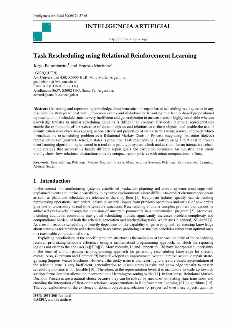
It is important to note that the number of logical facts in each state is variable, thereby in a given state can exist several facts which might not be necessarily present in another state definition. Such situation allows the approach to deal with (possibly) incomplete information about the schedule state or states described by different kind of relations in a straightforward and flexible way. Fig. 1 shows graphically the use of relational examples of schedule states belonging to an underlying RMDP (S1, S2, S3 in the figure) which is employed to model in a formal way the automated task rescheduling problem. In such a process, the learning agent employs relational representations to represent the states that he perceives as a result of successive applications of schedule repair operators (which represent the Actions of the RMDP, in this case Operator1, 2 and 3 in the figure), until a goal state is reached (SG in the figure). The definition of the relations that can take part in the state description an in the learned repair poli-cy are based on a set of rules that comprise Background Knowledge (BK), which is a key issue related to the in-ductive logic programming component present in the proposed approach, as we will see in further sections. BK consists of the definitions of general predicates that can be used in the induced relational hypotheses and it thus influences the concepts that can be represented.

Also, because first order representations are more expressive than attribute value representations the search space explored by inductive logic programming systems is much larger (and often infinite). To focus the search on the most relevant hypotheses and to eliminate useless hypotheses from the search space, it is necessary resorting to some kind of declarative bias mechanism. Declarative bias is implemented by means of so-called mode and type declarations. Therefore, in our approach, the optimal schedule repair policy is obtained through intensive simulation solving the underlying RMDP by resorting to a Relational Reinforcement Learning (RRL) algorithm [15], which is the relational version of model-free reinforcement learning algorithms such the well-known Q-Learning algorithm.

Figure 1. A graphical representation of an automated task rescheduling problem stated as a Relational Markov

Decision Process.

60 Inteligencia Artificial

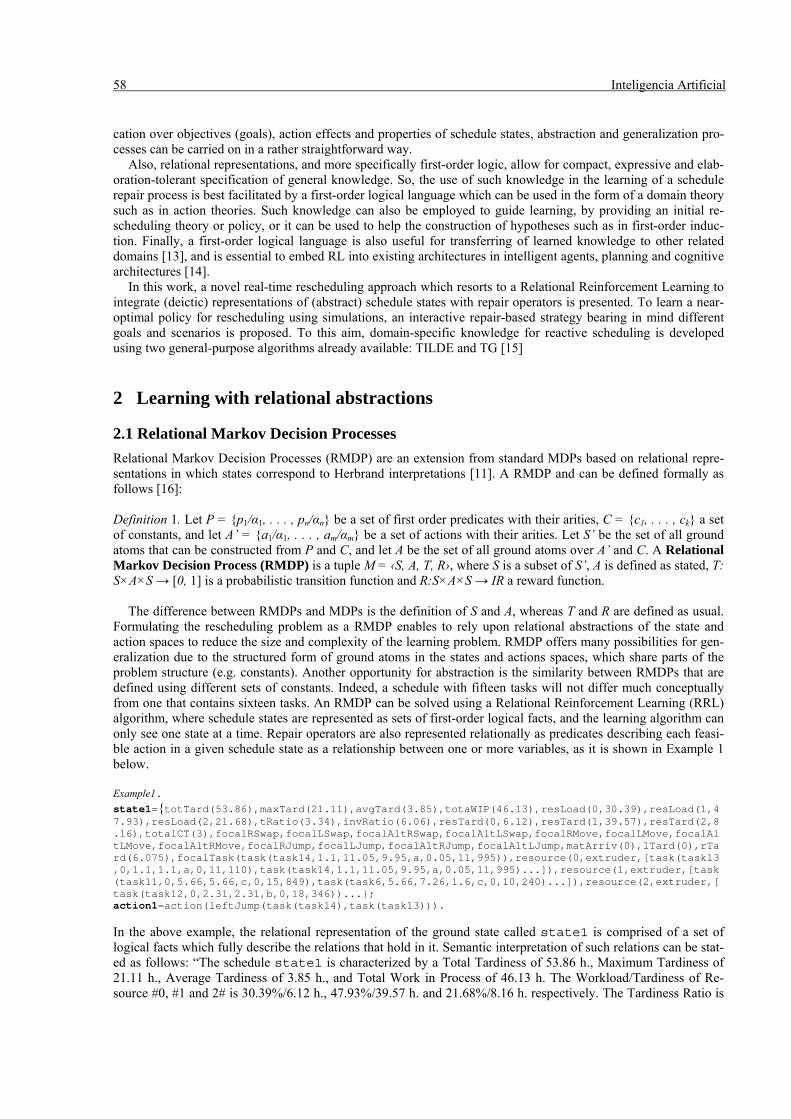
Figure 2. Adapted RRL algorithm for learning to repair schedules through schedule state transition simulation

(Algorithm 1) and state abstraction (Algorithm 2).

The integration of relational representations with MDPs is a promising approach to embed RL into more gen-eral cognitive production systems which use a logical representation level for knowledge, beliefs, intentions, goals and plans [17]. In such systems, RL is incorporated as a mechanism for learning skills or behaviors of a general cognitive agent including real-time rescheduling capabilities [14][18]. In this way, RRL algorithms are concerned with reinforcement learning in domains that exhibit structural properties and in which different kinds of related objects, namely tasks and resources exist [15][16][19]. This is usually characterized by a large and possibly un-bounded number of different states and actions as it is the case of planning and scheduling. Rather than using an explicit state−action Q-table, RRL stores the Q-values in a logical regression tree [20].

The relational version of the Q-learning algorithm is shown in Fig. 2 (Algorithm 1). So, BK is loaded before the training process starts and for each trial after the Q-function hypothesis has been initialized, the RRL algo-rithm starts learning episodes [15][21]. During each episode, all the visited abstract states and the selected actions are stored, together with the rewards related to each visited (abstract state, action)-pair. At the end of each epi-sode, when the system ends up in a goal state, it uses back-propagation of values/rewards and the current Q-function approximation to compute and update the corresponding Q-value approximation for each encountered (abstract state, action)-pair in the episode. The algorithm presents the set of (abstract state, action, qvalue)-triplets encountered in each learning episode to a relational regression engine, which will use this set of Examples to update the current regression tree for the Q-function. In order to accelerate and generalize the value function an abstract state induction is performed based on ground schedule states. Because of the relational representation of states and actions and the inductive logic programming component of the RRL algorithm, there must exist some body of background knowledge (BK) which is generally true for the entire domain to facilitate induction of ab-stract states and represent the repair policy in the form of Prolog rules. The computational implementation of the RRL algorithm has to deal successfully with the relational format for (states, actions)-pairs in which the examples are represented and the fact that the learner is given a continuous stream of (state, action, q-value)-triplets to learn predicting q-values for (state, action)-pairs during training.

The TILDE relational regression algorithm [19][21][22] is used in RRL to induce the membership function which allows obtaining the abstract-state corresponding to the ground state. Such function is used by Algorithm 2 in Fig. 2 which carries out this task, taking as parameters a ground state in relational format (See Example 1), the membership function induced by TILDE and BK, both as a collection of Prolog rules. Then for each rule avail-

Inteligencia Artificial 61 able in the algorithm creates an abstract state and adds it to a new collection. After that, it loads the BK and the collection of abstract states using the Prolog statement Consult. Later on, each abstract state is evaluated against the ground state that has been passed as a parameter by means of θ-subsumption; if such ground state is subsumed by the actual abstract state, the last is returned to Algorithm 1. If there is no abstract state which subsumes the ground state, Algorithm 2 returns an empty set. Finally, the TG algorithm is used for accumulating simulated ex-perience in a compact way at the end of each learning episode. This creates a readily available decision-making rule for generating a sequence of repair operators that are available at each visited abstract schedule state s.

2.2 Retrieving experience and membership values using relational regression trees

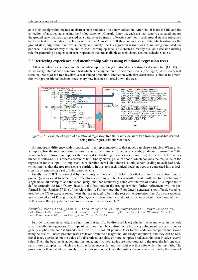
All accumulated experience and the membership function are stored in a first-order decision tree (FODT), in which every internal node contains a test which is a conjunction of first-order literals (See Fig. 3). Also, every leaf (terminal node) of the tree involves a real valued prediction. Prediction with first-order trees is similar to predic-tion with propositional decision trees: every new instance is sorted down the tree.

Figure 3. An example of a part of a relational regression tree (left) and a detail of two from ten possible derived

Prolog rules (right), without root query. An important difference with propositional tree representations is that nodes can share variables. When given

an input i, first the root node atom is tested against the example. If the test succeeds, producing substitution θ, the yes-branch is followed and applies the next test (substituting variables according to θ). If the test fails, the no-branch is followed. This process continues until finally arriving at a leaf node, which contains the real value of the regression for this input. An important consideration here is that there is a unique path leading to each leaf node, which implies that the tree represents a partition. In this approach logical decision trees are converted into a deci-sion list by employing a set of rules based on cuts.

Finally, the FODT is converted by the prototype into a set of Prolog rules that are used in execution time to predict Q-values and to select repair operators accordingly. The TG algorithm starts with the tree containing a single node, all examples and the Root Query, and then recursively completes the rest of nodes. It is important to define correctly the Root Query since it is the first node of the tree upon which further refinements will be per-formed in the “Update ” line of the Algorithm 1. Furthermore, the Root Query generates a set of basic variables used by the TG to execute several tests that are needed to build the rest of the regression tree. As a consequence, in the derived set of Prolog rules, the Root Query is present in the first part of the antecedent of each one of them. In this work, the query defined as a root is showed in the Example 2: Example 2. root((focal_Task(T), totalTardiness(W), maxTardiness(X), avgTardiness(Y), totalWorkInProcess(Z), tardinessRatio(A), inventoryRatio(B), totalCleanoutTime(F), focalTardiness(G), action_move(Cons,T,SF))).

In order to complete a node, the algorithm first tests (to be discussed later) whether the example set in the node is sufficiently homogeneous. This type of test should not be confused with the query refinement process. If homo-geneity applies, the node is turned into a leaf; if it is not, all possible tests for the node are computed and scored using heuristics. Theses possible tests are taken from the background knowledge definition, and they can be rela-tional facts, queries about the value of a discretized variable, or more complex predicates that can involve several rules. Then, the best test is added into the node, and two new nodes are incorporated to the tree: the left one con-tains those examples for which the test has been successful and the right one those for which the test fails. The procedure is then called recursively for the two sub-nodes. Once the instance arrives to a leaf node, the value of

62 Inteligencia Artificial that leaf is used as the prediction for that instance. The main difference between this algorithm and traditional decision tree learners relies in the generation of the tests to be incorporated into the nodes. To this aim, the algo-rithm employs a refinement operator ρ that works under θ-subsumption.

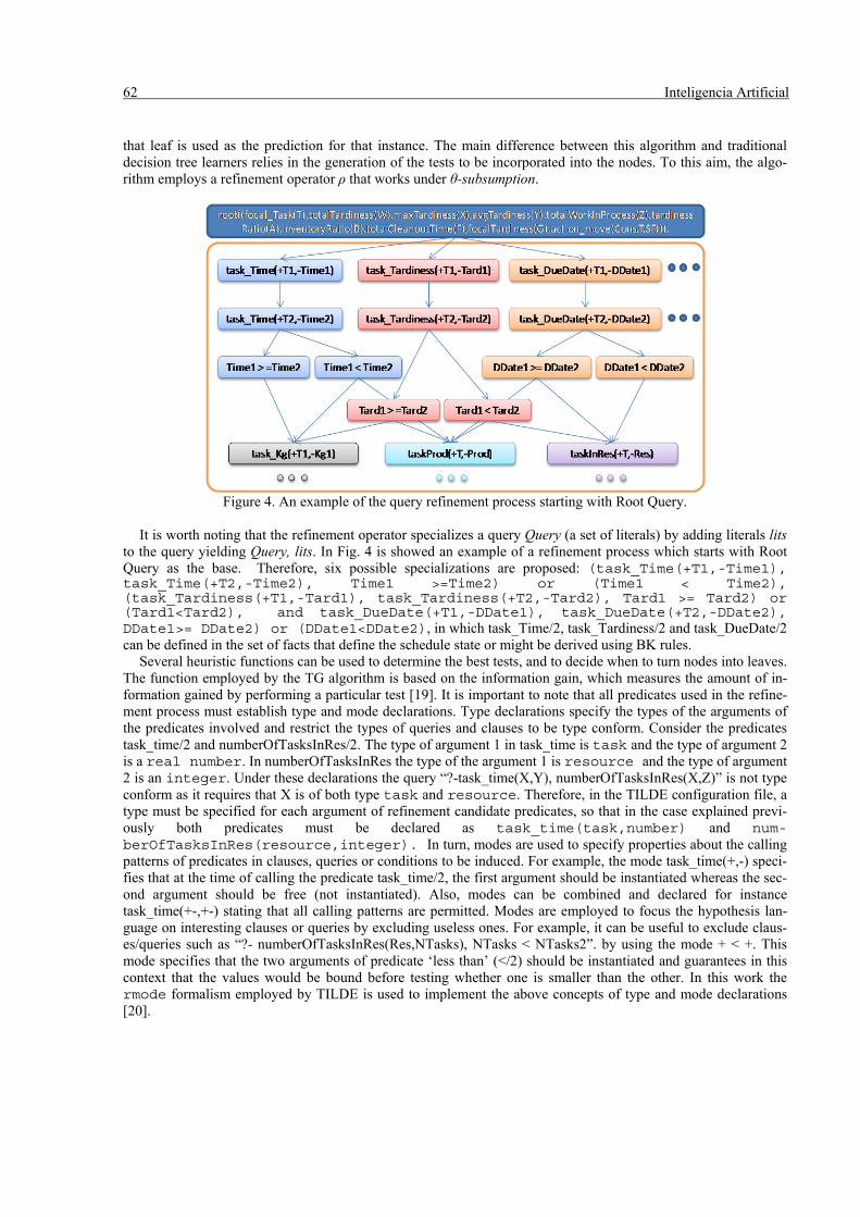
Figure 4. An example of the query refinement process starting with Root Query.

It is worth noting that the refinement operator specializes a query Query (a set of literals) by adding literals lits

to the query yielding Query, lits. In Fig. 4 is showed an example of a refinement process which starts with Root Query as the base. Therefore, six possible specializations are proposed: (task_Time(+T1,-Time1), task_Time(+T2,-Time2), Time1 >=Time2) or (Time1 < Time2), (task_Tardiness(+T1,-Tard1), task_Tardiness(+T2,-Tard2), Tard1 >= Tard2) or (Tard1<Tard2), and task_DueDate(+T1,-DDate1), task_DueDate(+T2,-DDate2), DDate1>= DDate2) or (DDate1<DDate2), in which task_Time/2, task_Tardiness/2 and task_DueDate/2 can be defined in the set of facts that define the schedule state or might be derived using BK rules.

Several heuristic functions can be used to determine the best tests, and to decide when to turn nodes into leaves. The function employed by the TG algorithm is based on the information gain, which measures the amount of in-formation gained by performing a particular test [19]. It is important to note that all predicates used in the refine-ment process must establish type and mode declarations. Type declarations specify the types of the arguments of the predicates involved and restrict the types of queries and clauses to be type conform. Consider the predicates task_time/2 and numberOfTasksInRes/2. The type of argument 1 in task_time is task and the type of argument 2 is a real number. In numberOfTasksInRes the type of the argument 1 is resource and the type of argument 2 is an integer. Under these declarations the query “?-task_time(X,Y), numberOfTasksInRes(X,Z)” is not type conform as it requires that X is of both type task and resource. Therefore, in the TILDE configuration file, a type must be specified for each argument of refinement candidate predicates, so that in the case explained previ-ously both predicates must be declared as task_time(task,number) and num-berOfTasksInRes(resource,integer). In turn, modes are used to specify properties about the calling patterns of predicates in clauses, queries or conditions to be induced. For example, the mode task_time(+,-) speci-fies that at the time of calling the predicate task_time/2, the first argument should be instantiated whereas the sec-ond argument should be free (not instantiated). Also, modes can be combined and declared for instance task_time(+-,+-) stating that all calling patterns are permitted. Modes are employed to focus the hypothesis lan-guage on interesting clauses or queries by excluding useless ones. For example, it can be useful to exclude claus-es/queries such as “?- numberOfTasksInRes(Res,NTasks), NTasks < NTasks2”. by using the mode + < +. This mode specifies that the two arguments of predicate ‘less than’ (</2) should be instantiated and guarantees in this context that the values would be bound before testing whether one is smaller than the other. In this work the rmode formalism employed by TILDE is used to implement the above concepts of type and mode declarations [20].

Inteligencia Artificial 63 3 Abstraction and Generalization in Rescheduling Domains The drawbacks and limitations of attribute-value (propositional) representations in learning a rescheduling policy discussed in previous sections are solved by our proposal by resorting to relational (or first-order) deictic repre-sentations. This approach relies on a language for expressing sets of relational facts that describe schedule states and repair actions in a compact and logical way; each state is thus characterized by only those facts that hold in it, which are obtained applying a hold(State) function. Formally, first-order representations are based on a relational alphabet Σ, which consists of a set of relation symbols P and a set of constants C. Each constant c ∈ C denotes an object (i.e. a task or resource) in the domain and each p/a ∈ P denotes either a property (or attribute, i.e. task tardi-ness) of some object (if a=1) or a relation between objects (for example, if a > 1, e.g. precedes(task1,task2)).

To represent structured terms in the schedule domain, e.g., resource(1,extruder(1),[task1,task2,task5]), the rela-tional alphabet is extended with a set of function symbols or functors F = {f1/α1, . . . , fk/αk} where each fi (i = 1 . . . k) denotes a function from Ck to C, where α is called the “arity” of the functor, and fixes the number of its argu-ments, e.g. precedes/2, task/5, averageTardiness/1, focalRightSwappability/0, among others. The prototype im-plements the concept of “learning from interpretations” in [19], so in this notation, each (state, action) pair will be represented as a set of relational facts, which is called a relational interpretation. In addition to a relational ab-straction, a deictic representation for describing schedule states and repair operators is proposed as a powerful alternative to scale up RRL in rescheduling problems. Deictic representations deal naturally with the varying number of tasks and resources in the planning world by defining a focal point for referencing objects (tasks and resources) in the schedule. This focal point is represented by a functor called focal/1, which takes one parameter to specify a task that fixes the repair scope and objectives. Such task is selected using different criteria, depending on the type of event which generates the disruption. Once this focal task is known, other facts that describe the schedule state and are relevant for repairing it can be established, such as leftTardiness/1 or altRightTardiness/1, among others. So, to characterize transitions in the schedule state due to repair actions, a deictic representation resorts to constructs such as: i) The first task in the new order, ii) The next task to be processed in the affected resource, and iii) Tasks and due date in a rush order at the top of the priority list.

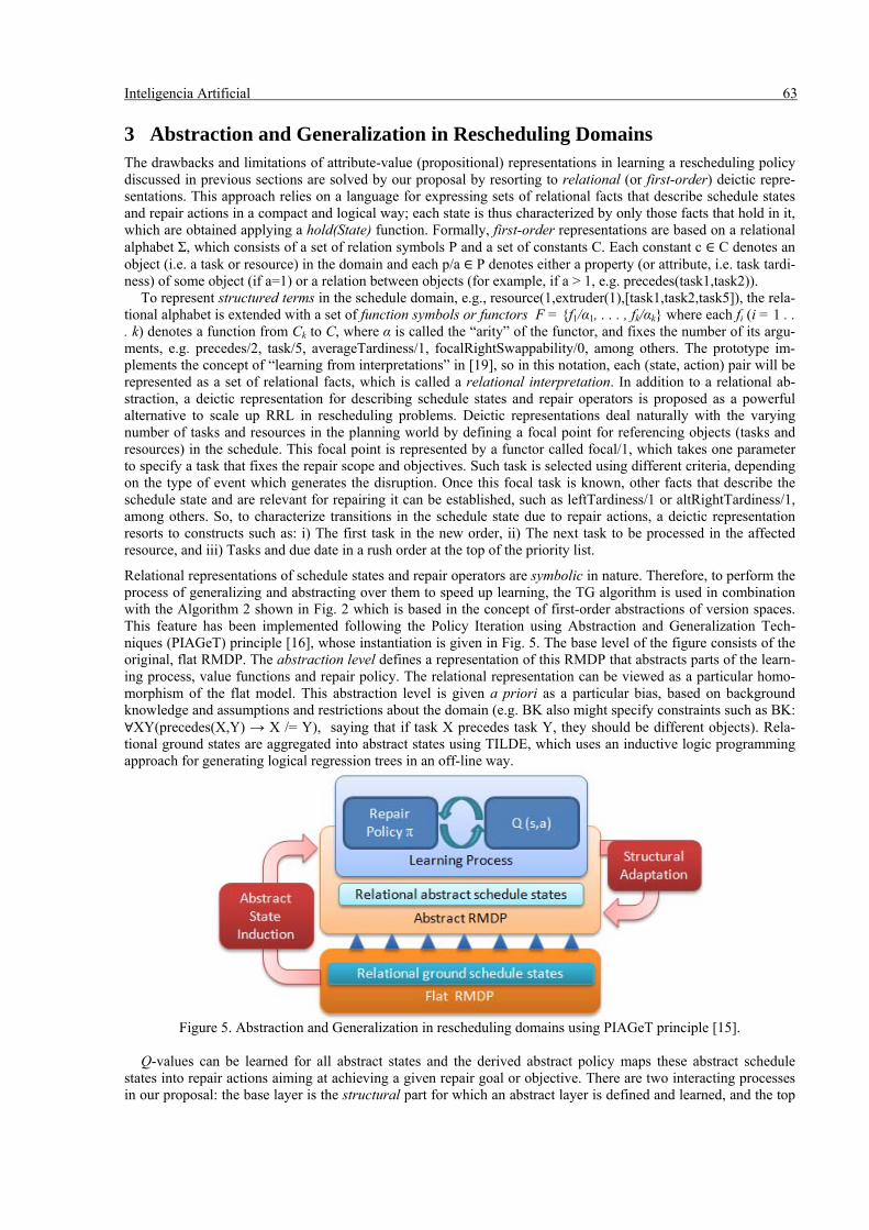
Relational representations of schedule states and repair operators are symbolic in nature. Therefore, to perform the process of generalizing and abstracting over them to speed up learning, the TG algorithm is used in combination with the Algorithm 2 shown in Fig. 2 which is based in the concept of first-order abstractions of version spaces. This feature has been implemented following the Policy Iteration using Abstraction and Generalization Tech-niques (PIAGeT) principle [16], whose instantiation is given in Fig. 5. The base level of the figure consists of the original, flat RMDP. The abstraction level defines a representation of this RMDP that abstracts parts of the learn-ing process, value functions and repair policy. The relational representation can be viewed as a particular homo-morphism of the flat model. This abstraction level is given a priori as a particular bias, based on background knowledge and assumptions and restrictions about the domain (e.g. BK also might specify constraints such as BK: ∀XY(precedes(X,Y) → X /= Y), saying that if task X precedes task Y, they should be different objects). Rela-tional ground states are aggregated into abstract states using TILDE, which uses an inductive logic programming approach for generating logical regression trees in an off-line way.

Figure 5. Abstraction and Generalization in rescheduling domains using PIAGeT principle [15].

Q-values can be learned for all abstract states and the derived abstract policy maps these abstract schedule

states into repair actions aiming at achieving a given repair goal or objective. There are two interacting processes in our proposal: the base layer is the structural part for which an abstract layer is defined and learned, and the top

64 Inteligencia Artificial layer that is responsible for learning a repair policy. Finally, the Structural Adaptation component is added so as to the defined structures are allowed to change as the learning process incorporates more training examples via simu-lation or through knowledge provided by experts in the form of BK rules. Example 3. ∀A,B,C,D(maxTard(A), precedes(B,C), precedes(C,D), A>57.8) is an Abstract State that denotes the set of schedules states in which the maximum tardiness A is greater than 57.8, where a task B precedes a task C, who in turns precedes the task D. Note that in this case, the task denoted by C must be the same in all cases where it appears.

As can be seen in Example 3, each abstract state models a set of interpretations of the underlying learning pro-cess (RMDP), and defines which relations should hold in each of the ground states it covers. Formally, this is expressed as a conjunction ≡ a ∧. . .∧ m of logical atoms, e.g., a logical query. The use of variables makes room for abstracting over specific domain objects as well. Thus, an abstract state is basically a logical sentence, specify-ing general properties of several states visited during learning through simulation of abstract state transitions. The action-value Q-function relies on a set of abstract states, which together encode the kind of rescheduling knowledge learned through state transition simulation in a compact and formal way, which can be used in real time to repair plans whose feasibility have been affected by disruptive events. Abstract state spaces compactly specify in a logical way a Relational Markov Decision Process state space S as a set of abstract states, and can be defined formally as follows [16]: Definition 2. Let Γ be a logical vocabulary and let be the set of all Γ-structures , a multi-part abstraction (MPA) over is a list , … , , where each (i =1 . . . n) (called a part) is a formula. A structure ∈ is covered by an MPA iff there exists a part (i =1 . . . n) such that |= . An MPA is a partition iff for all structures there is exactly one part that covers it. An MPA μ over Σ induces a set of equivalence classes over Σ, possibly forming a partition. MPAs are to be seen as sets. In other words, μ is a compact representation of a first-order abstraction level over Σ. An element σ ∈ Σ is covered by a part < > iff σ |= . Then, an abstract schedule state space is an MPA , … , , where each (i=1…n) is an abstract schedule state. An abstract schedule state action space is an MPA ⟨ , ⟩ … , ⟨ , ⟩ , i.e. a product-MPA over the schedule state-action space

. Definition 3. Let M = ‹S, A, T, R› be an RMDP. An abstract RMDP M is a structure ‹Z, A, T, R›. The abstract schedule state space Z = {Z1, . . . ,Zn} is a partition of the schedule state space S. Typically, |S| >> |Z|, offering a solution to many of the problems with large state spaces described previously. Let ψ denote the membership func-tion defined as ψ : S → Z, which maps each schedule state in the original space S to one of the sets in Z. Now each partition in Z is defined as Zi = {s | ψ(s) = Zi}. For all i, j = 1. . . n, Z satisfies the following properties: i) ⊆ , ii) ⋃ , and iii) Zi ∩ Zj = ∅, if i = j. Since we do not consider action-space abstraction, both M and M share the same action set A. A transition function and a reward function for M can now be defined in terms of T and R.

R Z , a ω s ∙ s, a (1)

T Z , a, Z ω s ∙ s, a, s′ (2)

To ensure that T and R are well-defined, a weighting function ∶ → 0,1 has been added, where for each , ∑ 1. The weighting expresses how much the state s contributes to the abstract state ZI =

ψ(s). The function is chosen to be in proportion to the state occupancy distribution using the TG algorithm online. Therefore, we learn an abstract policy Π which is defined as Π : Z → A such that π(s, a) = Π(ψ(s), a), for all s ∈ S, a ∈ A. So, in this approach it is necessary to induce an abstract schedule state space Z for which the Q-values and policies are learned. Q-learning on an abstract schedule state space is performed by updating an ab-stract action-value function based on the (ground) transition (st, at, rt, st+1) as follows:

, a : , a α γ ∙ max , a , a (3)

In this way, Q-values for abstract states are learned, and these Q-values are shared among all states that are mem-bers of the same abstract state (See Algorithm 1 in Fig. 2). Based on the presented RRL approach, the prototype

Inteligencia Artificial 65 generates the definition of the Q-function from a set of examples in the form of abstract state-action-value tuples, and dynamically makes partitions of the set of possible schedules states. These partitions are described by a kind of abstract schedule state, that is, a logical condition, which matches several real schedule states like the one in Example 3. The relational Q-learning approach sketched above thus needs to solve two tasks: finding the right partition and learning the right values for the corresponding abstract state-action pairs. The abstract Q-learning algorithm depicted in Fig. 2 starts from a partition of the state space in the form of a decision list of abstract state-action pairs , , … , , where is assumed that all possible abstract actions are listed for all abstract states . Each abstract state is a conjunctive query, and each abstract action contains a possibly variabilized action. The relational Q-learning algorithm now turns the decision list into the definition of the qvalue/1 predicate, and then applies Q-learning using the qvalue/1 predicate to rank state-action pairs. This means that every time a concrete state-action pair (s, a) is encountered, a Q-value q is computed using the current definition of qvalue/1, and then the abstract Q-function, that is, the definition of qvalue/1 is updated for the abstract state-action pair to which (s, a) belongs, which is performed using ψ. That is, the abstract state aggregates a set of state atoms into an equivalence class . Using this powerful abstraction procedure, schedule states are characterized by a set of common properties and the corresponding repair policy takes advantage of the problem structure and relations among objects in the schedule domain [10]. As a result, the rescheduling policy may be reused in somewhat simi-lar problems were the same relations apply, and without any further learning. As only fully observable worlds are considered, rescheduling knowledge is only due to abstracting schedules using relationships between world ob-jects. An abstract state covers a ground state s iff s |= , which is tested using θ-subsumption.

4 Industrial Case Study An example problem proposed in [23] is considered to illustrate our approach for automated task rescheduling. It consists of a batch plant which is made up of 3 semi-continuous extruders that process customer orders for four products (A,B,C and D). Each extruder has distinctive characteristics such that not all the extruders can process all products. Additionally, processing rates depend on both the extruder and the product being processed. For more realism, set-up times required for resource cleaning have been introduced, based on the precedence relationship between different types of final products. Processing rates and cleanout requirements are detailed in [23].

The prototype application has been implemented in Visual Basic.NET 2008 Development Framework 3.5 SP2 and SWI Prolog 6.0.2 running under Windows Vista. Also, the TILDE and TG modules from the ACE Datamin-ing System developed by the Machine Learning group at the University of Leuven [22] have been used. The pro-totype admits two modes of use: training and consult. During training it learns to repair schedules through simu-lated transitions of schedule states, and the generated knowledge is encoded in the Q-function. Exploitation of rescheduling knowledge is made in the consult mode. The disruptive events that the system can handle are the arrival of a new order/rush order to the production system, delay or shortage in the arrival of raw materials, and machine breakdown. Logical queries are processed by Prolog wrappers (.NET dynamic libraries), which made up a transparent interface between the .NET agent and the relational repair policy and objects describing schedule states. Before starting a training session the user must define through a graphical interface, the value of all simula-tion and training parameters, related to Initial schedule condition, Learning Parameters and Goal State Definition. The latter is a key parameter that has to be defined before starting a simulation since it establishes the desired repair goal. Training a rescheduling agent can be carried out by selecting one of three alternative goals, which is selected through an option list: Tardiness Improvement, Stability or Balancing. For example, in the case of Tardi-ness Improvement, credit assignment has the particularity of penalizing sequences of repair actions leading to a final state where the total tardiness is greater than the corresponding one to the initial schedule. In turn, Stability goal tries to minimize task movements in the repaired schedule with respect to the initial one, and Balancing is a mix between the foregoing two.

Order attributes correspond to product type, due date and size. In learning to insert an order, the rescheduling scenario is described by: i) arrival of an order with given attributes that should be inserted into a randomly gener-ated schedule state, and ii) the arriving order attributes are also randomly chosen. This way of generating both the schedule and the new order aims to expose the rescheduling agent to sensible different scenarios that allow it to learn a comprehensive repair policy to successfully face the environment uncertainty. Accordingly, the initial schedule is generated in terms of the next set of parameters which can be changed using the graphical interface of the prototype: Number of orders (randomly between [10,20]), Order composition, Order Size (an interval between 100 y 1000 kg) and Due Date.

The focal and global variables used in this example are shown in Example 1, in all cases training is carried out with a variable number of orders in a range of 10 to 15. In the situation considered, there exist a certain number of orders already scheduled in the plant and a new order must be inserted so as to meet the goal state for a repaired schedule. In each training episode, a random schedule state was generated, and a random insertion is attempted for

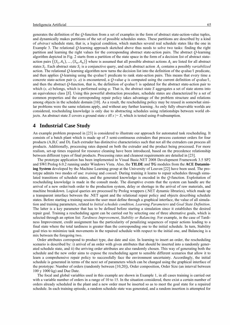
66 Inteligencia Artificial the new order (whose attributes are also randomly chosen), which in turn serves as the focal point for defining repair operators. Fig. 6 highlights results in the overall learning process, for each one of the available rescheduling goals. As can be seen, for Stability, the learning curve is flattened after approximately 350 episodes, when a near-optimal repair policy is obtained.

Figure 6. Learning curve for the Arrival of a new order event, with three different goals.

For the other two more stringent situations, namely Tardiness Improvement and Balancing, learning curves

tend to stabilize later, possibly due to a higher number of repair operations deemed necessary to try at early stages of learning so as to guarantee goal achievement. As it is shown in Fig.6, after 450 training episodes, only between 5 and 8 repair steps are required, on average, to insert a new order (regardless of the number of orders previously scheduled!).

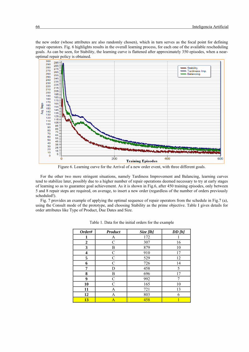
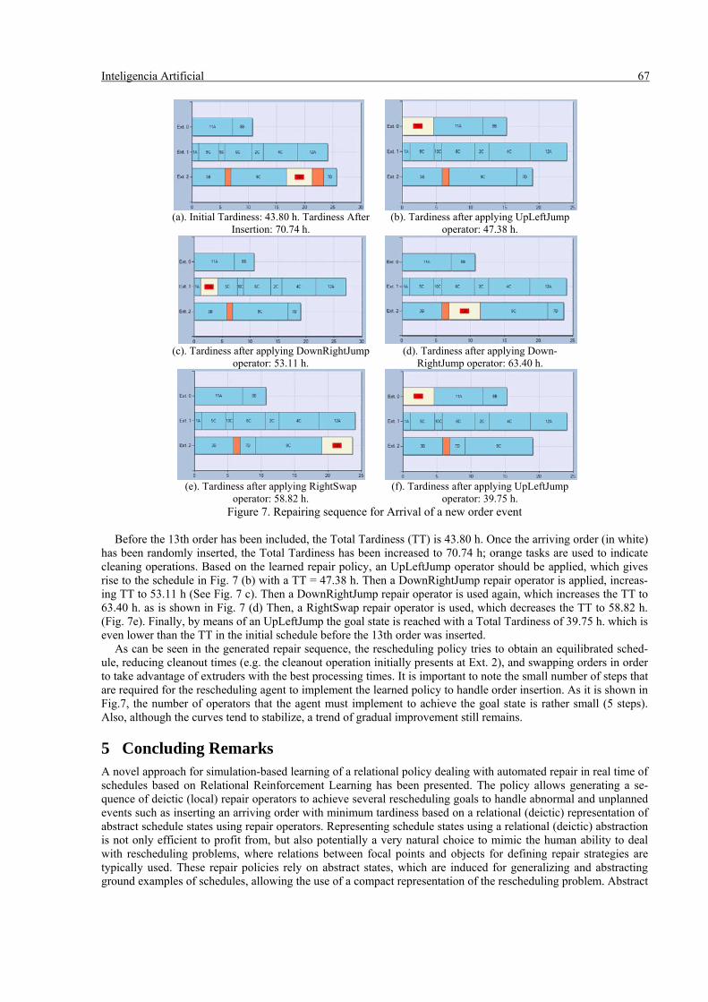
Fig. 7 provides an example of applying the optimal sequence of repair operators from the schedule in Fig.7 (a), using the Consult mode of the prototype, and choosing Stability as the prime objective. Table I gives details for order attributes like Type of Product, Due Dates and Size.

Table 1. Data for the initial orders for the example

Order# Product Size [lb] DD [h] 1 A 172 1 2 C 307 16 3 B 879 10 4 C 910 17 5 C 529 12 6 C 726 14 7 D 458 5 8 B 696 17 9 C 992 7

10 C 165 10 11 A 721 13 12 A 803 6 13 A 458 1

Inteligencia Artificial 67

(a). Initial Tardiness: 43.80 h. Tardiness After

Insertion: 70.74 h. (b). Tardiness after applying UpLeftJump

operator: 47.38 h.

(c). Tardiness after applying DownRightJump

operator: 53.11 h. (d). Tardiness after applying Down-

RightJump operator: 63.40 h.

(e). Tardiness after applying RightSwap

operator: 58.82 h. (f). Tardiness after applying UpLeftJump

operator: 39.75 h. Figure 7. Repairing sequence for Arrival of a new order event

Before the 13th order has been included, the Total Tardiness (TT) is 43.80 h. Once the arriving order (in white)

has been randomly inserted, the Total Tardiness has been increased to 70.74 h; orange tasks are used to indicate cleaning operations. Based on the learned repair policy, an UpLeftJump operator should be applied, which gives rise to the schedule in Fig. 7 (b) with a TT = 47.38 h. Then a DownRightJump repair operator is applied, increas-ing TT to 53.11 h (See Fig. 7 c). Then a DownRightJump repair operator is used again, which increases the TT to 63.40 h. as is shown in Fig. 7 (d) Then, a RightSwap repair operator is used, which decreases the TT to 58.82 h. (Fig. 7e). Finally, by means of an UpLeftJump the goal state is reached with a Total Tardiness of 39.75 h. which is even lower than the TT in the initial schedule before the 13th order was inserted.

As can be seen in the generated repair sequence, the rescheduling policy tries to obtain an equilibrated sched-ule, reducing cleanout times (e.g. the cleanout operation initially presents at Ext. 2), and swapping orders in order to take advantage of extruders with the best processing times. It is important to note the small number of steps that are required for the rescheduling agent to implement the learned policy to handle order insertion. As it is shown in Fig.7, the number of operators that the agent must implement to achieve the goal state is rather small (5 steps). Also, although the curves tend to stabilize, a trend of gradual improvement still remains.

5 Concluding Remarks A novel approach for simulation-based learning of a relational policy dealing with automated repair in real time of schedules based on Relational Reinforcement Learning has been presented. The policy allows generating a se-quence of deictic (local) repair operators to achieve several rescheduling goals to handle abnormal and unplanned events such as inserting an arriving order with minimum tardiness based on a relational (deictic) representation of abstract schedule states using repair operators. Representing schedule states using a relational (deictic) abstraction is not only efficient to profit from, but also potentially a very natural choice to mimic the human ability to deal with rescheduling problems, where relations between focal points and objects for defining repair strategies are typically used. These repair policies rely on abstract states, which are induced for generalizing and abstracting ground examples of schedules, allowing the use of a compact representation of the rescheduling problem. Abstract

68 Inteligencia Artificial states and macro-actions or operators for schedule repair facilitate and accelerates both learning and knowledge transfer, which is independent of the type of event that has generated a disruption and can be used reactively in real-time. Finally, an additional advantage provided by the relational (deictic) representation of schedule (abstract) states and operators is that, by relying on an appropriate and well designed set of background knowledge rules, it enables the automatic generation through inductive logic programming of heuristics that can be naturally under-stood by an end-user.

References

[1] G. Vieira, J. Herrmann and E. Lin. Rescheduling Manufacturing Systems: a Framework of Strategies, Poli-cies and Methods. J. of Scheduling, 6, 39, 2003.

[2] H. Aytug, M. Lawley, K. McKay, S. Mohan and R. Uzsoy. Executing production schedules in the face of uncertainties: A review and some future directions. European Journal of Operational Research, 161, 86–110, 2005.

[3] G. Henning. Production Scheduling in the Process Industries: Current Trends, Emerging Challenges and Op-portunities. Computer-Aided Chemical Engineering, 27, 23, 2009.

[4] A. Adhitya, R. Srinivasan and I. A. Karimi. Heuristic rescheduling of crude oil operations to manage abnor-mal supply chain events. AIChE J. 53(2), 397-422, 2007.

[5] K. Miyashita. Learning Scheduling Control through Reinforcements, International Transactions in Opera-tional Research, 7, 125, 2000.

[6] G. Zhu, J. Bard and G. Yu. Disruption management for resource-constrained project scheduling. Journal of the Operational Research Society, 56, 365-381, 2005.

[7] M. Zweben, E. Davis, B. Doun and M. Deale. Iterative Repair of Scheduling and Rescheduling. IEEE. Trans. Syst. Man Cybern., 23, 1588, 1993.

[8] Li, Z. and M. Ierapetritou. Reactive scheduling using parametric programming. AIChE J. 54(10), 2610-2623, 2008.

[9] K. Gersmann and B. Hammer. Improving iterative repair strategies for scheduling with the SVM. Neuro-computing, 63, 271–292, 2005.

[10] Eduardo F. Morales. Relational state abstraction for reinforcement learning. Proceedings of the Twenty-first Intl. Conference (ICML 2004), Banff, Canada, 2004.

[11] J. Palombarini and E. Martínez. SmartGantt – An Intelligent System for Real Time Rescheduling Based on Relational Reinforcement Learning. Expert Systems with Applications, 39, 10251- 10268, 2012.

[12] P. Tadepalli, R. Givan and K. Driessens. Relational Reinforcement Learning: An Overview. In Proceed-ings of the Workshop on Relational Reinforcement Learning at ICML’04, Banff, Canada, 2004.

[13] Eduardo F. Morales. Scaling up reinforcement learning with a relational representation. In Proceedings of the Workshop on adaptability in multi-agent systems at AORC’03, Sydney, Australia, 2003.

[14] S. Nason and J. E. Laird. Soar-RL: integrating reinforcement learning with Soar. Cognitive Systems Re-search, 6, 51–59, 2005.

[15] S. Džeroski, L. De Raedt and K. Driessens. Relational Reinforcement Learning. Machine Learning, 43, No. 1/2, p. 7, 2001.

[16] Martijn Van Otterlo. The Logic of Adaptive Behavior: Knowledge Representation and Algorithms for Adaptive Sequential Decision Making Under Uncertainty in First-order and Relational Domains, IOS Press, Amsterdam, 2009.

[17] Erik T. Mueller. Commonsense Reasoning, Morgan Kaufman Publishers, Amsterdam, 2006. [18] D. Trentesaux. Distributed control of production systems. Engineering Applications of Artificial Intelli-

gence, 22, 971–978, 2009. [19] Luc De Raedt. Logical and Relational Learning, Springer-Verlag, Berlin, 2008. [20] H. Blockeel and L. De Raedt. Top-down Induction of First Order Logical Decision Trees. Artificial Intel-

ligence, 101, No. 1/2, p. 285, 1998. [21] Richard Sutton and Andrew Barto. Reinforcement Learning: An Introduction, MIT Press, Boston, Mas-

sachusetts, 1998. [22] Kurt Driessens, Jan Ramon and Hendrick Blockeel: Speeding up Relational Reinforcement Learning

through the use of an Incremental First Order Decision Tree Learner. In: De Raedt, L. and Flach, P. (eds.) 13th Euro Conf. Machine Learning, vol. 2167, 97, Springer, 2001.

[23] R. Musier and L. Evans. An Approximate Method for the Production Scheduling of Industrial Batch Pro-cesses with Parallel Units. Comp. and Chem. Engineering, 13, 229, 1989.