Integrating spatial capture-recapture models with variable ... · density estimation, mark resight, noninvasive genetic sampling, spatial capture recapture a CC0 license. author/funder

1

Running head: Testing density estimation models 1

2

Integrating spatial capture-recapture models with variable 3

individual identifiability 4

5

JOEL S. RUPRECHT1,*, CHARLOTTE E. ERIKSSON

1, TAVIS D. FORRESTER2, DARREN A. CLARK

2, 6

MICHAEL J. WISDOM3, MARY M. ROWLAND

3, BRUCE K. JOHNSON2,†, AND TAAL LEVI

1 7

8

1Department of Fish and Wildlife, 104 Nash Hall, Oregon State University, Corvallis, OR 97331 9

2Oregon Department of Fish and Wildlife, 1401 Gekeler Lane, La Grande, OR 97850 10

3Pacific Northwest Research Station, USDA Forest Service, 1401 Gekeler Lane, La Grande, OR 11

97850 12

†Retired 13

*Email: [email protected] 14

15

Abstract. Many applications in ecology depend on unbiased and precise estimates of animal 16

population density. Spatial capture recapture models and their variants have become the 17

preferred tool for estimating densities of carnivores. Within the spatial capture-recapture family 18

are variants that require individual identification of all encounters (spatial capture-recapture), 19

individual identification of a subset of a population (spatial mark-resight), or no individual 20

identification (spatial count). In addition, these models can incorporate telemetry data (all 21

models) and the marking process (spatial mark-resight). However, the consistency of results 22

105 and is also made available for use under a CC0 license. (which was not certified by peer review) is the author/funder. This article is a US Government work. It is not subject to copyright under 17 USC

The copyright holder for this preprintthis version posted March 29, 2020. . https://doi.org/10.1101/2020.03.27.010850doi: bioRxiv preprint

https://doi.org/10.1101/2020.03.27.010850

2

among methods and the relative precision of estimates in a real-world setting are unknown. 23

Consequently, it is unclear how much and what type of data are needed to achieve satisfactory 24

density estimates. We tested a suite of models to estimate population densities of black bears 25

(Ursus americanus), bobcats (Lynx rufus), cougars (Puma concolor), and coyotes (Canis 26

latrans). For each species we genotyped fecal DNA collected with detection dogs. A subset of 27

individuals from each species were affixed with GPS collars bearing unique markings to be 28

resighted by remote cameras set on a 1 km grid. We fit 10 models for each species ranging from 29

those requiring no animals to be individually recognizable to others that necessitate full 30

individual recognition. We then assessed the contribution of incorporating telemetry data to each 31

model and the marking process to the mark-resight model. Finally, we developed an integrated 32

hybrid model that combines camera, physical capture, genetic, and GPS data into a single 33

hierarchical model. Importantly, we find that spatial count models that do not individually 34

identify animals fail in all cases whether or not telemetry data are included. Results improved as 35

models contained more information on individual identity. Models where a subset of individuals 36

were identifiable yielded qualitatively similar results, but can produce quantitatively divergent 37

estimates, suggesting that long-term population monitoring should use a consistent method 38

across years. Incorporation of telemetry data and the marking process can produce more accurate 39

and precise density estimates. Our results can be used to guide future study designs to efficiently 40

estimate carnivore densities for better understanding of population dynamics, predator-prey 41

relationships, and community assemblages. 42

Key words: abundance, black bear, bobcat, camera trapping, carnivore, count, cougar, coyote, 43

density estimation, mark resight, noninvasive genetic sampling, spatial capture recapture 44

45



https://doi.org/10.1101/2020.03.27.010850

3

INTRODUCTION 46

Population abundance is a state variable of paramount importance in both applied and 47

basic ecology but remains a challenge to estimate for most free-ranging animal populations. This 48

is particularly the case for terrestrial carnivore species that are cryptic and occur at low densities, 49

which preclude observational censuses or sightability-corrected survey methods (Wilson and 50

Delahay 2001). Many statistical models accounting for imperfect detection have been used to 51

estimate abundance, but the data required for each method vary along a continuum of recognition 52

of individual animals, ranging from no individual recognition to full individual recognition. For 53

data-poor situations in which no animals can be uniquely identified, models to estimate 54

abundance have been developed based on presence-absence of unmarked individuals in a 55

sampling session (Royle and Nichols 2003) or counts of unmarked individuals (Buckland et al. 56

1993, Royle 2004, Rowcliffe et al. 2008, Chandler and Royle 2013, Moeller et al. 2018). Other 57

models rely on partially-observable encounter histories when a subset of the population is 58

identifiable (e.g. White 1996, McClintock and White 2009, Sollmann et al. 2013a, Augustine et 59

al. 2018), and data-rich models utilize fully-observable encounter histories such that all 60

individuals can be uniquely identified (e.g., Otis et al. 1978, Nichols 1992, Royle et al. 2013). 61

Collecting higher resolution data where individuals are identifiable is substantially more 62

challenging, but models based on these data may produce more robust estimates of abundance, 63

particularly when the more demanding assumptions for data-poor models are violated (Chandler 64

and Royle 2013, Augustine et al. 2019). Knowing what type and how much data to collect to 65

achieve unbiased results with satisfactory precision, yet not beyond that required, is therefore a 66

central challenge to estimate population abundance for conservation, management, or research 67

objectives. 68



https://doi.org/10.1101/2020.03.27.010850

4

Spatial capture recapture (SCR; Borchers and Efford 2008, Royle and Young 2008) has 69

emerged as the most prominent method of abundance estimation for carnivores over the past five 70

years (Appendix S1: Fig. S1). SCR models exploit the spatial locations of animal detections and 71

assume the rate or probability an individual is detected is highest at its home range center and 72

declines as distance from the home range center increases (Royle and Young 2008). The 73

spatially-referenced detections of an individual allow the estimation of the animal’s activity 74

center, and the number of estimated activity centers yields an estimate of abundance. Population 75

density, often preferable to abundance, is calculated by dividing the estimated number of activity 76

centers by the area of the state space, which eliminates the arbitrarily defined effective sampling 77

area required in traditional capture-mark-recapture approaches (Royle et al. 2013). Furthermore, 78

SCR can accommodate individual and trap-level covariates to explain spatial and individual 79

variation in detection rates. 80

SCR models are well-suited for noninvasive genetic sampling in which individuals are 81

uniquely identified, typically using DNA from feces or hair samples, to produce fully-observable 82

encounter histories (Gardner et al. 2009, Kery et al. 2011, Morin et al. 2016, 2018). Scat-83

detection dogs in particular have become a common tool to efficiently collect feces on large 84

landscapes within a narrow time window to ensure demographic closure even for species that 85

occur at low densities (Wasser et al. 2004, 2011). While effective for SCR density estimation, 86

scat detection requires highly-trained dogs and specialization in genetic techniques or the 87

resources to contract out those tasks. As a more inexpensive and accessible alternative, wildlife 88

researchers increasingly use remote cameras to study and monitor wildlife. However, cameras 89

can only be used for conventional SCR analyses when all individuals of a species possess natural 90



https://doi.org/10.1101/2020.03.27.010850

5

markings (e.g. unique pelage patterns) that permit individual identification (but see Augustine et 91

al. 2018). 92

Spatial mark-resight (SMR) and generalized spatial mark-resight (gSMR) models are 93

variants of SCR that allow spatially-explicit density estimation when only a subset of the 94

population can be uniquely identified (Chandler and Royle 2013, Sollmann et al. 2013a, 95

Whittington et al. 2018). A common example is identification of individual study animals that 96

are collared (i.e., marked) from a population of interest. For many species it would be inefficient 97

to capture and mark animals solely for the purpose of density estimation; however, many 98

researchers and wildlife management agencies routinely monitor populations with telemetry 99

devices. In these cases, resighting marked animals on an array of remote cameras may offer a 100

relatively straightforward option for estimating density at little extra cost (Whittington et al. 101

2018). 102

Due to the challenge of individually marking animals, spatial count (SC) or ‘unmarked 103

SCR’ models (Chandler and Royle 2013) have been developed to exploit spatial autocorrelation 104

in counts of unmarked animals to make inference on their activity centers, and by extension, 105

population density. The attractiveness of this approach is that it requires no individual 106

identification so the population need not be artificially nor naturally marked. The only data 107

required for SC models are spatially-referenced counts of animal detections, which allows use of 108

standard camera trapping datasets that can be collected noninvasively without the cost and 109

specialized equipment needed for genotyping. Should SC models produce robust density 110

estimates as suggested by Chandler and Royle (2013) and Evans and Rittenhouse (2018), they 111

would represent a major advance in our ability to rapidly and affordably count carnivores. 112



https://doi.org/10.1101/2020.03.27.010850

6

These three model types require data of vastly different levels of individual identifiability 113

which raise concerns over the level of agreement in accuracy and precision with each technique. 114

Understanding the relative performance of these commonly-used density estimators is critical to 115

guide future population monitoring for conservation and management. We believe, a priori, that 116

genetic SCR methods yield the most robust density estimates because they have the strictest data 117

requirements in terms of individual identification. As the use of SMR and SC methods 118

proliferates in the literature, however, it is important to evaluate their credibility with respect to 119

the ‘gold standard’ SCR approach. A variety of additional data sources can be incorporated into 120

these models, which could potentially increase the concordance of results from data poor SC 121

models and data rich SCR models while also increasing precision and accuracy. For example, all 122

of these models can be informed by telemetry data (Sollmann et al. 2013a) to provide 123

independent estimates of home range size and location, and the SMR model can additionally be 124

informed by the capture-mark-recapture process used to mark animals (Whittington et al. 2018). 125

Since research projects and monitoring programs have limited budgets, it is also critical to know 126

how much and what type of data must be collected to achieve unbiased results with satisfactory 127

precision. 128

Here we use a unique dataset consisting of 1) genotyped scats located by detection dogs, 129

2) images of both marked and unmarked animals from an array of remote cameras, 3) encounter 130

histories of physical captures to mark animals, and 4) GPS (Global Positioning System) collar 131

locations to estimate the abundances of four carnivore species: black bears (Ursus americanus), 132

bobcats (Lynx rufus), cougars (Puma concolor), and coyotes (Canis latrans). Our objective is to 133

evaluate a suite of existing spatial density models across a spectrum of data richness to evaluate 134

agreement in results and precision. In addition, we develop a new hybrid model that can 135



https://doi.org/10.1101/2020.03.27.010850

7

incorporate SCR and SMR data sources (i.e. including genotypes, the physical marking process, 136

camera data, and GPS data) into a single hierarchical model, and assess the resulting gains in 137

precision. Notably our model comparisons occur in the context of a real system rather than 138

simulation. Each species varies in its life history, from highly territorial but group living 139

(coyotes), to non-territorial solitary individuals (black bears), to solitary territorial individuals 140

with territory size varying by sex (bobcat females are territorial while males are not; cougar 141

males are territorial while females are not). By evaluating a suite of methods with different data 142

requirements, our findings directly address how population densities of terrestrial carnivores can 143

most efficiently be estimated, and whether the investment in genotyping or marking and 144

resighting animals is necessary given the availability of models that do not rely on individual 145

identification. 146

147

METHODS 148

Study Area 149

Our study was conducted in and adjacent to the Starkey Experimental Forest and Range 150

(hereafter Starkey) in the Blue Mountains of northeastern Oregon (Fig. 1). Starkey is bounded by 151

a 2.4-meter fence, enclosing 100.7 km2, which prevents the passage of large herbivores 152

(Rowland et al. 1997); however, carnivores are undeterred by the fence and regularly cross in 153

and out of the enclosure (this study, Oregon Department of Fish and Wildlife, unpublished data). 154

Starkey is part of the Wallowa-Whitman National Forest and is administered by the US Forest 155

Service. Land immediately adjacent to Starkey is predominantly public and managed by the US 156

Forest Service (Wallowa-Whitman and Umatilla National Forests) but also includes private 157

inholdings. The study area contains a mosaic of Ponderosa pine (Pinus ponderosa) stands and 158



https://doi.org/10.1101/2020.03.27.010850

8

mixed pine-fir forests (Pinus, Abies and Pseudotsuga spp.), interspersed with grasslands 159

dominated by native bunchgrasses (Poa, Danthonia, and Pseudoroegneria spp.) and invasive 160

annual grasses (Bromus and Ventenata spp.) (Rowland et al. 1997). Elevation ranges between 161

1,122 and 1,500 m within Starkey (Rowland et al. 1997). See Wisdom et al. (2005) for additional 162

details about Starkey. 163

164

Data collection 165

Scat dataset 166

Scat detection dogs from the University of Washington Conservation Canine program 167

surveyed a 224 km2 study area encompassing all of Starkey and roughly an equal area 168

immediately to the north and west of the enclosure between 6 and 26 June 2017 (Fig. 1). The 169

area surveyed was composed of 56 gridcells each with an area of 4 km2. Detection dogs surveyed 170

6–8 km linear distance within each cell to distribute effort across the study area. Dog handlers 171

were not given specific survey routes but were encouraged to follow natural travel corridors such 172

as ridgelines, saddles, drainage bottoms, game trails, and fencelines. No more than 50% of the 173

distance traveled per gridcell was permitted to be on linear features such as trails or roads. When 174

scats were located, the handler recorded the GPS position and placed the entire scat in triplicate 175

paper bags. Within 72 hours of collection, scats were desiccated in a drying oven for 24 hours at 176

40°C (Murphy et al. 2000). Detection dogs in our study were trained to locate black bear, coyote, 177

cougar, and bobcat scats (Fig. 2c). 178

We used genotyping by amplicon sequencing (Eriksson et al. 2020) to identify unique 179

individuals with single-nucleotide polymorphisms (SNPs). Genotyping by amplicon sequencing 180

uses the power of high-throughput sequencers to yield high genotype success rates and low error 181



https://doi.org/10.1101/2020.03.27.010850

9

rates. Coyote scats were genotyped following methods in Eriksson et al. (2020). We genotyped 182

bobcat, cougar, and black bears feces using the same approach but with novel primers designed 183

and tested specifically for this study (Appendix S2). Prior to genotyping, the identity of the 184

defecator for each scat was identified using DNA metabarcoding of ~100bp of the mtDNA 12S 185

region as part of a separate diet study (primers used in Eriksson et al. 2020, Massey et al. 2020, 186

and modified from Riaz et al. 2011). See Appendix S2 for single-nucleotide polymorphism 187

discovery methods and Eriksson et al. (2020) for detailed genotyping protocol. 188

189

Camera dataset 190

A 1- x 1-km grid of 94 unbaited remote cameras (Bushnell TrophyCam Aggressor, 191

Overland, KS) was placed inside the Starkey fence perimeter and was operational between April 192

and September 2017 (Fig. 1). All cameras were pointed north. We visited each camera station 193

every 6-8 weeks to change batteries and download data. Each camera was set to take a burst of 3 194

photos when triggered. 195

Photos were tagged to species or to individual when animals were uniquely identifiable 196

due to GPS collars and ear tags. We used the open source photo management software DigiKam 197

(www.digikam.org) for tagging and database management and the R library camtrapR (Niedballa 198

et al. 2016) to extract metadata from photos. We censored photos in which we could not 199

determine whether an animal was wearing a GPS collar or if we could not verify the identity of 200

an animal photographed with a GPS collar. However, these records constituted < 5% of all 201

detections. Because animals were typically photographed more than once during a visit, we 202

recorded information for each independent photo sequence and considered photo sequences more 203

than 30 minutes from the next detection of the same species to be independent. 204



https://doi.org/10.1101/2020.03.27.010850

10

205

Telemetry dataset 206

We captured and GPS-collared each of the four carnivore species as part of concurrent 207

research on predator-prey relationships. Coyotes were captured in Starkey using padded foothold 208

traps (Oneida Victor SoftCatch No. 3, Euclid, OH) with a tranquilizer tab (Balser 1965) 209

containing 50 mg propriopromazine hydrochloride attached to each trap to subdue captured 210

animals until researchers arrived. Captured animals were immobilized with tiletamine-zolazepam 211

(Telazol®) at a concentration of 10 mg/kg. A GPS collar (Lotek MiniTrack, Lotek Wireless Inc., 212

Newmarket, ON, Canada or Vectronic Vertex, Vectronic Aerospace GmbH, Berlin, Germany) 213

was placed on each adult coyote and was programmed to record locations every 2 or 3 hours. 214

We captured bobcats in Starkey using cage traps baited with visual and olfactory 215

attractants or incidentally in foothold traps intended for coyotes. Captured bobcats were 216

administered ketamine (10 mg/kg) and xylazine (1.5 mg/kg) for immobilization, and upon 217

release, yohimbine (0.125 mg/kg; Yobine®) was given as an antagonist for xylazine. Each 218

bobcat was fit with a GPS collar (Lotek MiniTrack, Lotek Wireless Inc., Newmarket, ON, 219

Canada) scheduled to take fixes every 2 hours. 220

Black bears were captured within Starkey using culvert traps or padded foot snares 221

(Lemieux and Czetwertynski 2006). Captured bears were immobilized with Telazol® at a 222

concentration of 7 mg/kg. Bears were fit with GPS collars (Lotek GPS 7000 or LiteTrack Iridium 223

420, Lotek Wireless Inc., Newmarket, ON, Canada) that recorded positions every 15 min to 2 224

hours. 225

We captured cougars using trained pursuit hounds. We searched for fresh cougar tracks in 226

snow and when located, released hounds to pursue tracks until the cougar was treed. Our search 227



https://doi.org/10.1101/2020.03.27.010850

11

area consisted of Starkey plus a buffer of approximately 20 km. Roads within this buffer were 228

searched as randomly as possible and dogs were allowed to pursue tracks of any individual. 229

When treed, cougars were immobilized with ketamine (10 mg/kg) and xylazine (2 mg/kg) via 230

dart gun, and before release administered yohimbine (0.125 mg/kg; Yobine®) as an antagonist 231

for xylazine. A GPS collar (Lotek GPS 4400S, IridiumTrack M, Lotek Wireless Inc., 232

Newmarket, ON, Canada or Vectronic Vertex Lite, Vectronic Aerospace GmbH, Berlin, 233

Germany) was placed on each cougar and was programmed to record locations every 3 hours. 234

We permanently marked the belting of GPS collars with unique numbers used to identify 235

individuals on camera (Fig. 2d). When possible (i.e. for the larger collars), we also affixed 236

sections of colored heat-shrink plastic tubing over the collar belting to assist with identification 237

(Fig 2a). We also ear tagged each captured animal such that females received ear tags on the left 238

ear and males on the right ear which allowed an additional cue when identifying GPS-collared 239

animals on camera. 240

We collected biological samples from each captured individual to match the genotypes of 241

GPS-collared animals with genotypes detected by scat detection dogs. For each animal we 242

sampled some combination of tissue, hair, and feces (see Eriksson et al. 2020 for additional 243

details). All animal handling was performed in accordance with protocols approved by the 244

USDA Forest Service, Starkey Experimental Forest Institutional Animal Care and Use 245

Committee (IACUC No. 92-F-0004; protocol #STKY-16-01) and followed the guidelines of the 246

American Society of Mammalogists for the use of wild mammals in research (Sikes 2016). 247

248

Modelling Approach 249



https://doi.org/10.1101/2020.03.27.010850

12

Our approach was to fit a suite of spatially-explicit models across a spectrum of data 250

resolutions (Table 1, Fig. 3) for each species to evaluate the value of each data source and to test 251

whether incorporating additional data improved precision. Each model considered here is a 252

variation of a conventional SCR model (Royle and Young 2008) in which the detection 253

probability ��,� (or rate ��,�) decays as a function of the Euclidean distance between the detector j 254

and the activity center s for individual i, di,j, to yield 255

��,� � �0�,� � ��,�/2�� , (1) 256

where �0�,� is the baseline detection probability when the detector is located exactly at the 257

activity center of the home range, and � is a spatial scale parameter related to home range size 258

that determines the rate at which detection probability declines with distance from the activity 259

center. The location of each activity center is latent but estimated as the centroid (spatial 260

average) of the detections for each individual. 261

The observed encounter histories ��,� can be modeled as either a binomial or Poisson 262

random variable, depending on whether the detection process yields binary or count outcomes, 263

��,�~ ��,� � �� , �� or ��,�~ ��,� � �� , (2) 264

where K is the number of sampling occasions, and �� is the data augmentation parameter that can 265

take the values of 0 or 1 (see below). Data augmentation is used to estimate the number of 266

animals in the state space, S (an area prescribed to be sufficiently large such that animals with 267

activity centers at the outermost regions of this area have a negligible probability of being 268

detected). �� determines whether each hypothetical individual in the augmented population is real 269

or not and is governed by a Bernoulli distribution, 270

�� ~ �� !�, (3) 271



https://doi.org/10.1101/2020.03.27.010850

13

in which ! is the expected number of activity centers divided by the augmented population size, 272

M, described above. The estimated population size N (i.e. the number of activity centers in the 273

state space) is then determined by summing over all �� , 274

" � ∑ �� , (4) 275

and density D is obtained by dividing the population size by the area of the state space, S, 276

D = N/S. (5) 277

We assumed a homogenous point process for the distribution of activity centers (s) such 278

that the x and y dimensions of each activity center were uniformly distributed within the defined 279

limits of the state space: 280

��,� ~ ��$��%�,�, %�,�� (6) 281

��,� ~ ��$��%�,�, %�,�� (7) 282

Each model subsequently described is based on the same framework as the conventional 283

SCR described above but involves variations due to different data sources or resolutions which 284

are described next. 285

286

Spatial Count or ‘unmarked SCR’ 287

The spatial count model (Chandler and Royle 2013) does not require individual recognition, so 288

the encounter history ��,�is replaced by a vector of counts of unmarked individuals at each 289

detector (��) and encounter rate � replaces p. The counts are now modeled as a Poisson random 290

variable, 291

�� ~ ��Λ� � �� (8) 292

where 293

Λ� � �0�,� ∑ ��,�/2�� . (9) 294



https://doi.org/10.1101/2020.03.27.010850

14

295

Spatial Mark-Resight 296

Spatial mark-resight models (Chandler and Royle 2013, Sollmann et al. 2013a) combine 297

SCR and SC. Here, a subset of the population is individually recognizable due to either natural or 298

artificial markings but the remaining individuals are observed without individual identity. The 299

Poisson distributed encounter history �. ��(��,� 300

�. ��(��,�~ ��. ��)*+�,� � �� (10) 301

is obtained for marked individuals and the resulting expected resighting rate �. ��)*+�,� 302

�. ��)*+�,� � �0. ��)*+�,� � ��,�/2�� (11) 303

is applied to the counts of unmarked individuals �� by replacing �0�,� in Eq. 9 with 304

�0. ��)*+�,�. An assumption of this model is therefore that marked and unmarked individuals 305

have the same rate of detection. 306

307

Generalized Spatial Mark-Resight 308

Generalized spatial mark-resight (gSMR; Whittington et al. 2018) is identical to the 309

conventional SMR described above but incorporates a submodel for the marking (i.e. physical 310

capture and tagging) process and is therefore suitable only when a portion of the population is 311

captured and marked. Generalized SMR alleviates bias introduced due to heterogeneity of 312

individual encounter rate arising from situations when the marked portion of the population 313

resides nearer to the resighting detectors (and are therefore detected more frequently) than 314

unmarked individuals at the periphery of the state space (Whittington et al. 2018). That is, it 315

accounts for the fact that the marked segment of the population is seldom distributed randomly 316



https://doi.org/10.1101/2020.03.27.010850

15

throughout the state space (Whittington et al. 2018). The marking process submodel is itself a 317

SCR model for the encounter histories of individuals captured and marked, �. ��(��)�,�, 318

�. ��(��)�,�~ ��. ��(��)�,� � �� , �� (12) 319

where the probability of capturing individual i in trap j similarly decays with distance according 320

to 321

�. ��(��)�,� � �0. ��(��)�,� � ��,�/2�� . (13) 322

The animal capture and marking process and the resighting of marked animals on cameras 323

(SMR) shares information on �� , si, and possibly �, which has the potential to increase model 324

performance and precision. 325

326

Hybrid Spatial Capture Recapture + Generalized Spatial Mark-Resight 327

In situations in which SCR data are obtained concurrently with a capture and marking 328

effort, and the marked individuals are resighted on an array of detectors (e.g. trail cameras), we 329

propose data from all three processes can be modeled together in a ‘hybrid’ SCR + gSMR model. 330

This model incorporates equations 1-7, and 10-13. In this data-rich model, the encounter 331

histories from each of the three data sources must be aligned such that each individual known 332

from either the marking/resighting process or scat detection process corresponds to the same 333

individual, i. in the combined model. However, not all known individuals are likely to be 334

detected in all data sources. For marked animals which are known to exist because they were 335

physically captured, the possible outcomes of the detection process are 1) detected by neither 336

camera nor genetics, 2) detected by camera only, 3) detected by genetics only, or 4) detected by 337

both camera and genetics. For unmarked animals (i.e. those not physically captured), the possible 338

outcomes of the detection process are 1) detected by neither camera nor genetics, 2) detected by 339



https://doi.org/10.1101/2020.03.27.010850

16

genetics only (and without a genotype matching any of the marked individuals), 3) detected by 340

camera only without individual identity, and 4) detected by camera and genetics (and without the 341

possibility of deterministically linking the genotype to the photographed individual). Information 342

on �� , si, and � can be shared, and baseline detection rates can be informed by the different data 343

sources when an individual is detected by one but not all detection methods. For example, 344

knowing a captured animal exists but was not detected by genetics can help inform the 345

probability of detection in the genetic SCR component. Similarly, knowing a captured animal 346

exists but was not photographed informs the detection probability for the SMR model 347

component. 348

349

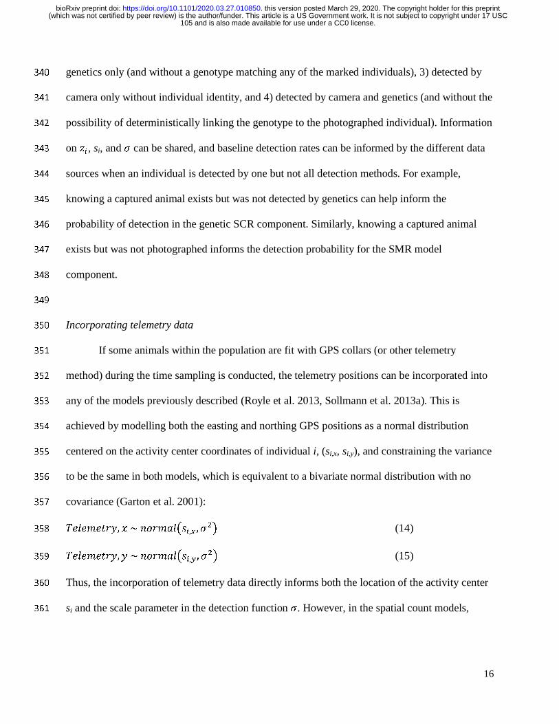
Incorporating telemetry data 350

If some animals within the population are fit with GPS collars (or other telemetry 351

method) during the time sampling is conducted, the telemetry positions can be incorporated into 352

any of the models previously described (Royle et al. 2013, Sollmann et al. 2013a). This is 353

achieved by modelling both the easting and northing GPS positions as a normal distribution 354

centered on the activity center coordinates of individual i, (si,x, si,y), and constraining the variance 355

to be the same in both models, which is equivalent to a bivariate normal distribution with no 356

covariance (Garton et al. 2001): 357

,��+��, � ~ ��-��,�, ��. (14) 358

,��+��, � ~ ��-��,�, ��. (15) 359

Thus, the incorporation of telemetry data directly informs both the location of the activity center 360

si and the scale parameter in the detection function �. However, in the spatial count models, 361



https://doi.org/10.1101/2020.03.27.010850

17

individual recognition is not known, which prevents the GPS data from being linked to specific 362

individuals, so in those models the telemetry data only inform �. 363

364

Application 365

For each of the four study species (black bear, bobcat, cougar, coyote), SC models were 366

fit using camera data. Individual identity was ignored in SC models even when it was known so 367

that we could evaluate an approach that required no individual recognition. SMR and gSMR 368

models were constructed from the same camera data as the SC models but GPS-collared animals 369

were identified to individual, with the latter method also including the encounter histories from 370

the marking process. SCR models were constructed only from genetic samples (scats) because 371

we could not identify individuals from cameras unless they were artificially marked. The gSMR 372

+ SCR hybrid model that we developed combined cameras, physical capture histories, and 373

genetic samples. We assumed that camera and scat data were independent because 1) both data 374

collection methods passively sampled the population in different ways and at different sites 375

within the superpopulation, 2) the detection of a scat did not influence the probability of that 376

individual being detected by camera (and vice-versa), and 3) neither camera placements nor scat 377

dog survey routes were influenced by the knowledge gained from the other method. 378

For every modeling method implemented (Table 1, Fig. 3), we fit models both with and 379

without GPS data. When telemetry data were included, we randomly selected 100 GPS locations 380

(Fig. 2b) to alleviate lack of independence arising from temporal autocorrelation. 381

For the genetic SCR analyses, we used a single occasion because detection dogs only 382

surveyed each gridcell once. We overlaid a 1 x 1 km grid over the survey area and attributed the 383

location of any scat inside that cell to the gridcell center. We modeled the effect of the survey 384



https://doi.org/10.1101/2020.03.27.010850

18

distance of the scat dog route within each gridcell on p0 (Eq. 1) using a linear model with a logit 385

link. Samples belonging to the same individual that were found in the same gridcell were 386

recorded as a single detection of individual i. Because some carnivore species defecate 387

nonrandomly as a means of scent marking, we believe removing recaptures within the same 388

gridcell helped ensure independence of samples. 389

For camera analyses, we parsed the encounter data into ten 14-day occasions beginning 390

15 April. We multiplied the detection function by the proportion of the occasion that each 391

camera was operational so that nonfunctioning cameras would not contribute to the model’s 392

likelihood. Similarly, if an animal marked at some point during the sampling period was not 393

available to be detected during one or more occasions due to collar loss, death, or because it was 394

not yet collared, we did not allow that individual to contribute to the likelihood for that occasion. 395

We initially sought to include sex-specific detection and scale parameters but abandoned 396

the effort because we had insufficient data on sex for SC and SMR models. Including sex-397

specific parameters for some but not all models would make meaningful comparisons difficult 398

given our primary interest was to compare inference between model types. 399

To ensure that we included a sufficiently large state space and number of augmented 400

individuals, for each species and model we ensured that M was substantially higher than the 401

estimated N, that the upper bound of ! was not near 1, and that the buffer around the survey area 402

which formed the state space was > 2.5 times σ. 403

To assess and compare dispersion across model types, we calculated the coefficient of 404

variation as the posterior standard deviation divided by the posterior mean. We refer to precision 405

as the inverse of the coefficient of variation rather than the inverse of the variance. 406

407



https://doi.org/10.1101/2020.03.27.010850

19

Model implementation 408

We conducted Markov Chain Monte Carlo (MCMC) simulations to estimate the posterior 409

distributions for the parameters of interest in all models. We used JAGS (Plummer 2003) in 410

program R version 3.6.1 (R Development Core Team 2019) and the jagsUI package (Kellner 411

2015). For each model we ran 3 parallel chains consisting of 10,000 iterations per chain and 412

discarded the first 9,000 as burn in. We assessed model convergence by visually inspecting 413

traceplots and ensuring the /0 values were less than 1.1 (Gelman 1996). If models failed to 414

converge after the first run, we updated them until convergence was satisfactory. For all 415

parameters, we calculated the 95% highest posterior density intervals (HPDI) and 95% Bayesian 416

credible intervals (BCI) (Chen and Shao 1999). For estimates of population size or density, 417

which may be sensitive to the amount of data augmentation prescribed, we report the posterior 418

mode in the text but also present the posterior means and medians in tables. 419

420

RESULTS 421

Our capture efforts yielded GPS collars placed on 6 black bears, 4 bobcats, 6 cougars, 422

and 9 coyotes that were able to be resighted and remained within the bounds of the state space 423

during the time camera and scat sampling occurred. We obtained 124 independent photo 424

sequences for bears (26 marked, 98 unmarked), 34 photo sequences of bobcats (9 marked and 25 425

unmarked), 48 photo sequences of cougars (24 marked, 24 unmarked), and 479 photo sequences 426

of coyotes (55 marked, 424 unmarked; Table 1). Scat dogs located 86 bear scats, 107 bobcat 427

scats, 18 cougar scats, and 772 coyote scats. Of these, we successfully genotyped 43 bear scats 428

out of 72 attempts (60% success rate), 86 bobcat scats out of 95 attempts (91% success rate), 15 429

cougar scats out of 17 attempts (88% success rate), and 201 coyote scats out of 216 attempts 430



https://doi.org/10.1101/2020.03.27.010850

20

(93% success rate). After removing duplicate scats from the same individual in the same gridcell, 431

we had 40 bear scats from 31 individuals, 68 bobcat scats from 32 individuals, 13 cougar scats 432

from 7 individuals, and 165 coyote scats from 83 individuals (Table 1). 433

All models converged such that /0 was less than 1.1 except for the bobcat SC model not 434

informed by telemetry, which after nearly 30 days of runtime had still not converged. Other SC 435

models without telemetry were slow to converge, exhibited poor mixing of chains, and were 436

possibly unstable. 437

Telemetry Data 438

Across all species and methods, the inclusion of GPS data resulted in a mean decrease in 439

the posterior modes for animal densities of 2.4% (Fig. 4, Appendix S3: Tables S1–S4). For all 440

methods except spatial count models, including GPS data led to a mean decrease in the 441

coefficients of variation of 19.9% (Fig. 5, Appendix S3: Tables S1–S4). But in spatial count 442

models, including GPS data increased the coefficients of variation by an average of 144.0% (Fig. 443

5, Appendix S3: Tables S1–S4). However, very low SC+GPS density estimates were responsible 444

for the increases in the coefficients of variation in those models—standard deviations were 445

actually smaller in SC models including GPS data. 446

Spatial Capture Recapture 447

We report SCR+GPS estimates as the benchmark to which the other methods are 448

compared because they are the most data-rich models of the methods tested. The SCR+GPS 449

estimate of the posterior mode (and 95% BCI) for black bears was 9.1/100 km2 (6.1–18.6 /100 450

km2); for bobcats was 12.1/100 km2 (8.4–16.2/100 km2), for cougars was 1.7/100 km2 (0.9–451

3.6/km2); and for coyotes was 25.4/100 km2 (21.0–30.9/100 km2) (Fig. 4, Appendix S3: Tables 452

S1–S4). 453



https://doi.org/10.1101/2020.03.27.010850

21

Spatial Count 454

Spatial count models produced highly divergent results depending on whether telemetry 455

data were included (Fig. 4; Appendix S3: Tables S1–S4). When GPS data were not included, 456

densities from SC models were on average 795.8% higher than SCR+GPS estimates (Fig. 4, Fig. 457

6). However, when GPS data were included, densities from SC models were on average 78.1% 458

lower than SCR+GPS estimates (Fig. 4, Fig. 6). Coefficients of variation for SC and SC+GPS 459

models were 75.1% or 243.1% greater than SCR+GPS, respectively (Fig. 5, Appendix S3: 460

Tables S1–S4). 461

Spatial Mark-Resight vs Spatial Capture Recapture 462

On average, SMR+GPS models estimated animal densities that were only 7.3% lower 463

than SCR+GPS models (Fig. 4, Fig. 6, Appendix S3: Table S1–S4). Coefficients of variation 464

were 49.3% higher in SMR+GPS models than SCR+GPS models (Fig. 5, Appendix S3: Tables 465

S1–S4). 466

Spatial Mark-Resight vs Generalized Spatial Mark-Resight 467

Across all models and species, adding the marking process to SMR models (i.e. SMR vs 468

gSMR) decreased estimates of animal density by an average of only 0.9% (Fig. 4, Fig. 6, 469

Appendix S3: Tables S1–S4). However, the coefficients of variation were on average 15.3% 470

lower in gSMR models than SMR models (Fig. 5, Appendix S3: Tables S1–S4). 471

Spatial Capture Recapture vs Hybrid 472

The Hybrid+GPS models estimated, on average, densities that were only 3.0% lower than 473

SCR+GPS models (Fig. 4, Fig. 6, Appendix S3: Tables S1–S4). The coefficients of variation 474

were 24.8% lower in the Hybrid+GPS model than the SCR+GPS model (Fig. 5, Appendix S3: 475

Tables S1–S4). 476



https://doi.org/10.1101/2020.03.27.010850

22

477

DISCUSSION 478

Many applications in ecology depend on unbiased and precise estimates of animal 479

density. Despite tremendous advancements in wildlife monitoring technology (e.g. remote 480

cameras), molecular methods (e.g. genotyping), and statistics (e.g. models accounting for 481

imperfect detection), estimating population density can still be a formidable task. Biased or 482

imprecise density estimates may at best lead to faulty inference and at worst put populations at 483

risk due to misguided conservation or management efforts. We found that SMR models based on 484

resighting marked animals on cameras produced density estimates consistent with genetic SCR 485

models for bears and cougars, but there was some divergence for bobcats for which the posterior 486

mode of SCR estimates were on average 78.4% higher than the SMR results and for coyotes for 487

which SCR estimates were on average 22.1% lower than the SMR results. For both species, the 488

posterior mode of the SCR models was contained in both the 95% HPDI and BCI of SMR 489

models, but the converse was not true (Fig. 4, Appendix S3: Tables S2 and S4). In contrast, SC 490

models reliant on photos of unmarked animals produced highly divergent density estimates. For 491

all four species, we observed the same pattern in which spatial count models without GPS data 492

exhibited positive bias and spatial count models with GPS data exhibited negative bias compared 493

to models with individual recognition. Informing σ with telemetry data did not lead to accurate 494

enumeration of activity centers and instead falsely attributed unmarked photo detections to too 495

few individuals. 496

SC models require sufficiently close trap spacing so that spatial autocorrelation can be 497

detected and used to identify activity centers (Chandler and Royle 2013). Poor density estimation 498

from SC models can result from insufficient spatial structure of animal detections that prevent 499



https://doi.org/10.1101/2020.03.27.010850

23

individual activity centers from being clearly demarcated. However, our 1 km camera grid 500

spacing allowed for many cameras per animal home range, suggesting that these models are not 501

robust for carnivores even with relatively ideal conditions. Further, SC results can be unreliable, 502

unstable, or suffer from convergence failure when data are sparse (Chandler and Royle 2013, 503

Ramsey et al. 2015, Kane et al. 2015, Burgar et al. 2018a, Burgar et al. 2018b, Murphy et al. 504

2018b), suggesting that this will be a consistent challenge in carnivore studies using unbaited 505

cameras within a time frame over which demographic closure can be reasonably assumed. 506

Recent work has also shown that populations with large values of σ can produce biased results in 507

SC models (Augustine et al. 2019). Including habitat covariates that influence spatial density 508

may in some cases offset bias (e.g. Evans and Rittenhouse 2018), but our results suggest that 509

fully unmarked SCR models (i.e. SC) are often unsuitable for density estimation of the 510

carnivores we studied, particularly when detectors are widely spaced, count data are sparse, and 511

auxiliary data are not available. Given the poor performance of SC models in our analysis, with 512

or without inclusion of telemetry data, we do not recommend this method be used for carnivore 513

species that cannot be uniquely identified in photographs. 514

Although SMR models and SCR models produced qualitatively similar density estimates, 515

the moderate divergence in results for bobcats and coyotes may be due to challenges when 516

simultaneously camera trapping for multiple species with distinct habitat preferences, home 517

range sizes, and life history strategies. Based on GPS data, bobcats in this system used dense 518

forest cover and our camera placements were biased away from this habitat type because they 519

had extremely limited viewsheds that would limit photos of other species. In contrast, detection 520

dogs readily located bobcat scats and the higher detection probability and sample size of scats 521

may have driven the difference in results between cameras and genetics. Although SCR 522



https://doi.org/10.1101/2020.03.27.010850

24

estimates were 78.4% higher than SMR estimates for bobcats, the discrepancy only amounted to 523

a difference of 5-6 individuals/100 km2. The disagreement could also be explained if detection 524

dogs found scats from bobcat kittens that were not detected on camera. Because bobcats can give 525

birth nearly year-round (Winegarner and Winegarner 1982), we cannot discount the possibility 526

that kittens were recruited during the time of sampling. 527

For coyotes, the discrepancy between SMR and SCR models may involve unmodeled 528

sources of individual heterogeneity in detection rates across methods as was observed by 529

Murphy et al. (2018a) who estimated lower densities when models were constructed solely from 530

scat data than from both scat and hair. The authors speculated that the behavioral status of 531

coyotes (i.e. resident vs transient) led to cohorts that were disproportionately detected using one 532

detection method over another. Specifically, they reasoned that territorial resident coyotes could 533

be more likely to be detected from scats because of smaller home ranges and increased scent-534

marking with scat for territorial defense than wide-ranging transients. Our study may exhibit an 535

analogous issue if cameras detected both resident and transient coyotes at high rates but the 536

detected scats disproportionately belonged to residents. 537

Similarly, Morin et al. (2016) suggested that SCR density estimation in coyotes could be 538

improved by modeling heterogeneity in σ and baseline detection rates arising as a result of 539

behavioral status. Without modelling heterogeneity, the bimodality in home range size can lead 540

to estimates of detection and scale parameters that are averaged between the two behavioral 541

states (Murphy et al. 2018). To explore whether failing to acknowledge these sources of 542

heterogeneity were responsible for the divergent results between SMR and SCR models, we 543

conducted a post-hoc analysis where σ and baseline detection parameters were allowed to vary as 544

a function of transient or resident behavioral status (see Appendix S4 for details). Including 545



https://doi.org/10.1101/2020.03.27.010850

25

behavioral status increased the estimates of density in both SMR+GPS and SCR+GPS models 546

but reduced the difference between them from 22% to 16% (Fig. 7). We thus speculate that the 547

unmodeled heterogeneity arising from the distinct behavioral states drove some but not all of the 548

disagreement between model types. 549

Previous studies have successfully estimated population densities of multiple carnivore 550

species using camera trapping (Jiménez et al. 2017, Burgar et al. 2018a, Rich et al. 2019). Our 551

study also suggests a multi-species monitoring approach is possible yet highlights the challenges 552

of simultaneous density estimation of multiple species. For example, the substantial variation in 553

home range size among carnivores requires fine-scale sampling for smaller ranges (e.g. coyotes 554

and bobcats) while allowing for the larger extents needed for greater home range sizes (e.g. bears 555

and cougars). This can be accomplished with either a finely-spaced grid (this study) or through 556

cameras that are clustered with variable spacing intervals (Rich et al. 2019, Murphy et al. 2019). 557

Similarly, assumptions of demographic closure may be challenging to meet for larger home 558

range species unless the extent of the study area is large enough to contain many home ranges. 559

For example, our small survey area relative to the species with the largest home range (e.g. only 560

7 distinct cougars were sampled from genetics) may have made our estimates sensitive to the 561

assumption of demographic closure given that the death, dispersal, or recruitment of even one 562

individual could have a substantial influence on estimates. 563

For all species, the inclusion of telemetry data to inform density estimation generally 564

produced consistent results with increased precision and smaller coefficients of variation for all 565

methods except spatial count models (Fig. 5, Appendix S3: Tables S1–S4). The gains in 566

precision were greatest for the models/species with the sparsest data (e.g. cougar SCR model). 567

Inclusion of GPS data for coyotes increased precision but led to consistently lower density 568



https://doi.org/10.1101/2020.03.27.010850

26

estimates across methods because 3 nonresident transient coyotes with very large territories 569

inflated estimates of σ, which in turn reduced density estimates. This highlights the challenge of 570

estimating σ when telemetry data are excluded and spatial recaptures are sparse. For example, 571

transient individuals with large home ranges may rarely or never be recaptured, which would 572

falsely suggest low detectability rather than the large value for σ that is evident from telemetry 573

data. The absence of telemetry data can thus lead to both imprecise and biased estimates of σ 574

with consequent effects on other model parameters (i.e. �0 or �0 and N) (Whittington et al. 575

2018). Improving the estimate of σ by incorporating telemetry data should aid in identifiability 576

of other parameters and lead to greater accuracy in the models incorporating GPS data. SC 577

models were particularly problematic because they produced biologically unrealistic density 578

estimates that changed from very high to very low with the inclusion of telemetry data. Although 579

telemetry data decreased precision in SC models, the large reduction in the density estimate 580

when including telemetry data led to an increase in the coefficient of variation because the 581

denominator became smaller. A highly biased result with high precision or low CV invites the 582

possibility of overconfidence in an incorrect result when using SC models. 583

Models that included more information on individual identity had more precise density 584

estimates (Fig. 5), except when the number of genotyped scats was very low. In particular, the 585

small sample of cougar scats led to SCR models that were substantially less precise than SMR 586

models (Fig. 5, Appendix S3: Table S4). For all species, the hybrid model containing camera, 587

physical capture (gSMR), and genetic (SCR) data had the lowest coefficients of variation (Fig. 5) 588

highlighting the benefit of leveraging multiple datasets even if some are sparse. 589

A recent movement in ecological modeling of demographic rates has sought to strengthen 590

inference by leveraging multiple data sources (e.g. Besbeas et al. 2002, Schaub et al. 2007). The 591



https://doi.org/10.1101/2020.03.27.010850

27

data required for SMR and SCR models require a substantial investment of time and money and 592

typically result in sparse data. Integrating multiple sparse data sources is thus an efficient use of 593

resources in addition to the benefits of improving precision and reducing bias. Others have 594

integrated camera and genetic data for spatially-explicit density estimation (Sollmann et al. 595

2013b, Clare et al. 2017, Gopalaswamy et al. 2012), but to our knowledge this has only occurred 596

when animals on camera could always be identified to individual, so the result was a SCR model 597

composed of two different data sources. This contrasts with our approach of combining SMR for 598

a partially-marked population (i.e. those in which not all individuals can be uniquely identified) 599

with genetic SCR data in which every sample was identifiable to individual. 600

Ancillary data associated with genetic or mark-resight data may motivate the decision to 601

collect one data type over another. For example, telemetry data obtained in conjunction with a 602

mark-resight study may be useful not only to inform σ and si, but also to classify an animal into a 603

behavioral state such as resident vs transient or breeder vs nonbreeder, and these distinctions 604

may explain important sources of individual heterogeneity in detection rate. The photographs in 605

a mark-resight analysis may also permit identification of juveniles which can easily be censored 606

if the researcher desires to estimate the density of the adult population segment only. While 607

genetic sampling is unlikely to yield these sources of information, it offers other benefits such as 608

the ability to study diet (e.g. Kartzinel et al. 2015), hormone levels (e.g. Gobush et al. 2014), and 609

population structure or genetic diversity (e.g. Goosens et al. 2005), which if useful for other 610

objectives may steer researchers toward that method of data collection. Genetic samples also 611

readily yield the sex of the individual which may not be possible from camera trapping for 612

species that are not sexually dimorphic. The cost of each data collection method may also play a 613

factor in the decision. While both genetics and mark-resight studies may be expensive, when a 614



https://doi.org/10.1101/2020.03.27.010850

28

segment of the population is already being monitored via telemetry devices, the extra cost to 615

resight marked individuals using cameras may be minimal compared to the cost of a separate 616

genetics SCR study (Whittington et al. 2018). However, in the absence of an existing effort to 617

obtain telemetry data, genetic SCR methods are substantially more cost effective given the 618

expense associated with capturing, collaring, and resighting animals. 619

We could likely refine our results by modeling species-specific sources of individual 620

heterogeneity as for coyotes (Fig. 7). For example, density estimates for species with disparate 621

home ranges sizes between sexes may improve by incorporating sex-specific detection and 622

spatial scale parameters (Sollmann et al. 2011). We chose not to, however, because information 623

on sex was not available for spatial count models and was only partially observable for mark-624

resight methods (i.e. for the marked animals only) because the sexes of our study species could 625

not accurately be determined from photos alone. Our approach was to standardize models as 626

much as possible across species for the purpose of comparing data sources and model 627

formulations and this precluded us from considering species-specific nuances beyond the 628

illustrative example for resident and transient coyotes (Fig. 7). 629

Another extension to our efforts might implement spatial partial identity models to 630

extract even more information from the existing datasets (Augustine et al. 2018). This would 631

allow partial genotypes (Augustine et al. 2019) or photos in which the marked status or 632

individual identity (Augustine et al. 2018, Jiménez et al. 2019) cannot be ascertained to be 633

included in SCR estimation. However, this model extension would minimally influence our 634

results because of the high genotyping success from scats using genotyping by amplicon 635

sequencing (Eriksson et al. 2020) and our relatively high success in identifying marked status or 636

individual identity in our camera trap photos. 637



https://doi.org/10.1101/2020.03.27.010850

29

Knowing how much and what type of data to collect is a challenge confronted by most 638

researchers aiming to efficiently estimate population densities. Our results from a suite of 639

spatially-explicit models for bears, bobcats, cougars and coyotes in a natural system highlight the 640

relative performances of models within the spatial capture recapture family constructed from 641

data of varying sources and resolutions. We acknowledge that in some instances, absolute 642

population densities may not be essential and simply being able to accurately characterize 643

relative changes in trends may be adequate. This may be the case for setting management 644

objectives for common species. In other cases, such as the calculation of extinction risk for 645

imperiled species, getting the most accurate estimates of population size is crucial. We found that 646

the most common method for estimating population size of terrestrial carnivores in the past five 647

years was (spatial) capture recapture and that only a minority of studies used methods that do not 648

require individual recognition (Appendix S1: Fig. 1). This suggests that in most cases, 649

researchers are willing to spend the resources necessary to achieve robust results. Regardless, the 650

method chosen must be commensurate with the objective of the study. 651

We conclude by suggesting that future research employing SCR or its variants to estimate 652

the density of carnivores (1) not use SC models, (2) use consistent methods among years because 653

variation in density estimates between SMR and SCR could be misinterpreted as population 654

change, (3) incorporate GPS data when possible, and (4) consider combining multiple data 655

sources using the hybrid SMR+SCR model presented here. We note that SCR models with few 656

scats produced density estimates consistent with, but less precise than, a years-long effort to 657

capture carnivores and resight them on camera traps. Given the inadequacy of SC models and 658

expense associated with capturing carnivores to mark them for resighting, we recommend that 659

new studies to estimate population density of carnivores (that are not distinguishable with natural 660



https://doi.org/10.1101/2020.03.27.010850

30

markings) first consider using genetic SCR. The efficacy to do so will continue to increase as 661

noninvasive genetic sampling transitions toward low-cost and high-success genotyping of SNPs 662

by high-throughput sequencing (Eriksson et al. 2020). Finally, newer models to estimate density 663

using unmarked animals, such as the time-to-event and space-to-event family of models (Moeller 664

et al. 2018), provide hope for a cost-effective method to estimate population densities for 665

multiple species. These models will require a similar field test to that presented here prior to their 666

integration into large-scale carnivore monitoring programs. 667

668

ACKNOWLEDGMENTS 669

We thank M. Bianco, K. Bowman, C. Brown, L. Carr, L. Chodelski, T. Craddock, E. Crain, C. 670

Eckrich, M. Esquibel, S. Gillman, M. Goldman, A. Hilger, R. Jensen, C. Kidd, M. Olsen, J. 671

Smith, A. Yancey, and J. Yancey for field support. We thank K. Cronin, S. Gillman, M. 672

Goldman, J. Hart, V. Heilman, R. Jensen, J. Neeley, N. Owen, S. Muñoz for photo tagging 673

support. We thank J. Allen for lab work. We thank R. Chandler and B. Augustine for coding 674

assistance. We thank B. Dick, R. Kennedy, and D. Rea and the USDA Forest Service Pacific 675

Northwest Research Station for logistical support. Funding and/or field equipment was provided 676

from Oregon Hunter’s Association, Oregon Trapper’s Association, Wildlife and Sportfish 677

Restoration Act, Pittman Robertson Act, Oregon Department of Fish and Wildlife, USDA Forest 678

Service, and Oregon State University. 679

680

681



https://doi.org/10.1101/2020.03.27.010850

31

LITERATURE CITED 682

Augustine, B. C., J. A. Royle, M. J. Kelly, C. B. Satter, R. S. Alonso, E. E. Boydston, and K. R. 683

Crooks. 2018. Spatial capture–recapture with partial identity: an application to camera traps. The 684

Annals of Applied Statistics 12:67–95. 685

686

Augustine, B. C., J. A. Royle, S. M. Murphy, R. B. Chandler, J. J. Cox, and M. J. Kelly. 2019. 687

Spatial capture–recapture for categorically marked populations with an application to genetic 688

capture–recapture. Ecosphere 10:e02627. 689

690

Balser, D. S. 1965. Tranquilizer tabs for capturing wild carnivores. The Journal of Wildlife 691

Management 29:438–442. 692

693

Besbeas, P., S. N. Freeman, B. J. T. Morgan, and E. A. Catchpole. 2002. Integrating 694

mark‐recapture‐recovery and census data to estimate animal abundance and demographic 695

parameters. Biometrics 58:540–547. 696

697

Borchers, D. L., and M. G. Efford. 2008. Spatially explicit maximum likelihood methods for 698

capture–recapture studies. Biometrics 64:377–385. 699

700

Buckland, S. T., D. R. Anderson, K. P. Burnham, and J. L. Laake. 1993. Distance sampling: 701

estimating abundance of biological populations. Oxford University Press, Oxford, UK. 702

703



https://doi.org/10.1101/2020.03.27.010850

32

Burgar, J. M., A. C. Burton, and J. T. Fisher. 2019. The importance of considering multiple 704

interacting species for conservation of species at risk. Conservation Biology 33:709–715. 705

706

Burgar, J. M., F. E. Stewart, J. P. Volpe, J. T. Fisher, A. C. Burton. 2018b. Estimating density for 707

species conservation: Comparing camera trap spatial count models to genetic spatial capture-708

recapture models. Global Ecology and Conservation 15:e00411. 709

710

Chandler, R. B., and J. A. Royle. 2013. Spatially explicit models for inference about density in 711

unmarked or partially marked populations. The Annals of Applied Statistics 7:936–954. 712

713

Chen, M. H. and Q. M. Shao. 1999. Monte Carlo estimation of Bayesian credible and HPD 714

intervals. Journal of Computational and Graphical Statistics 8:69–92. 715

716

Clare, J., S. T. McKinney, J. E. DePue, and C. S. Loftin. 2017. Pairing field methods to improve 717

inference in wildlife surveys while accommodating detection covariance. Ecological 718

Applications 27:2031–2047. 719

720

Eriksson, C. E., J. Ruprecht, and T. Levi. 2019. More affordable and effective noninvasive SNP 721

genotyping using high-throughput amplicon sequencing. bioRxiv. 722

https://doi.org/10.1101/776492. 723

724

Evans, M. J., and T. A. Rittenhouse. 2018. Evaluating spatially explicit density estimates of 725

unmarked wildlife detected by remote cameras. Journal of Applied Ecology 55:2565–2574. 726



https://doi.org/10.1101/2020.03.27.010850

33

727

Gardner, B., J. A. Royle, and M. T. Wegan. 2009. Hierarchical models for estimating density 728

from DNA mark–recapture studies. Ecology 90:1106–1115. 729

730

Garton, E. O., M. J. Wisdom, F. A. Leban, and B. K. Johnson. 2001. Experimental design for 731

radiotelemetry studies. Pages 15–42 in J. Millspaugh and J. Marzluff, editors. Radiotelemetry 732

and animal populations. Academic Press, San Diego. 733

734

Gelman, A. 1996. Inference and monitoring convergence. Pages 131–143 in W. R. Gilks, S. 735

Richardson and D. J. Spiegelhalter, editors. Markov chain Monte Carlo in practice. Chapman and 736

Hall/CRC, Boca Raton, Florida, USA. 737

738

Gobush, K. S., R. K. Booth and S. K. Wasser. 2014. Validation and application of noninvasive 739

glucocorticoid and thyroid hormone measures in free‐ranging Hawaiian monk seals. General and 740

Comparative Endocrinology 195:174– 182. 741

742

Goossens, B., L. Chikhi, M. F. Jalil, M. Ancrenaz, I. Lackman‐Ancrenaz, M. Mohamed, P. 743

Andau, and M. W. Bruford. 2005. Patterns of genetic diversity and migration in increasingly 744

fragmented and declining Orangutan (Pongo pygmaeus) populations from Sabah, Malaysia. 745

Molecular Ecology 14:441– 456. 746

747



https://doi.org/10.1101/2020.03.27.010850

34

Gopalaswamy, A. M., J. A. Royle, M. Delampady, J. D. Nichols, K. U. Karanth, and D. W. 748

Macdonald. 2012. Density estimation in tiger populations: combining information for strong 749

inference. Ecology 93:1741–1751. 750

751

Jiménez, J., J. C. Nuñez-Arjona, C. Rueda, L. M. González, F. García-Domínguez, J. Muñoz-752

Igualada, and J. V. López-Bao. 2017. Estimating carnivore community structures. Scientific 753

Reports 7:1–10. 754

755

Kane, M. D., D. J. Morin, and M. J. Kelly. 2015. Potential for camera-traps and spatial mark-756

resight models to improve monitoring of the critically endangered West African lion (Panthera 757

leo). Biodiversity and Conservation 24:3527–3541. 758

759

Kartzinel, T. R., P. A. Chen, T. C. Coverdale, D. L. Erickson, W. J. Kress, M. L. Kuzmina, D. L. 760

Rubenstein, W. Wang, and R. M. Pringle. 2015. DNA metabarcoding illuminates dietary niche 761

partitioning by African large herbivores. Proceedings of the National Academy of Sciences of 762

the United States of America 112:8019– 8024. 763

764

Kellner, K. F. jagsUI: A wrapper around rjags to streamline JAGS analyses. R package version 765

1.3.1. 2015. 766

767

Kery, M., B. Gardner, T. Stoeckle, D. Weber and J. A. Royle. 2011. Use of spatial 768

capture‐recapture modeling and DNA data to estimate densities of elusive animals. Conservation 769

Biology 25:356–364. 770



https://doi.org/10.1101/2020.03.27.010850

35

771

Lemieux, R., and S. Czetwertynski. 2006. Tube traps and rubber padded snares for capturing 772

American black bears. Ursus, 17:81–92. 773

774

Massey, A. L., G. Roffler, T. Vermeul, J. M. Allen, and T. Levi. 2019. Comparison of 775

mechanical sorting and DNA metabarcoding for diet analysis with degraded wolf scats. bioRxiv. 776

https://doi.org/10.1101/2019.12.13.875898. 777

778

McClintock, B. T., and G. C. White. 2009. A less field‐intensive robust design for estimating 779

demographic parameters with mark–resight data. Ecology 90:313–320. 780

781

Moeller, A. K., P. M. Lukacs, and J. S. Horne. 2018. Three novel methods to estimate abundance 782

of unmarked animals using remote cameras. Ecosphere 9:e02331. 783

784

Morin, D. J., M. J. Kelly, and L. P. Waits. 2016. Monitoring coyote population dynamics with 785

fecal DNA and spatial capture–recapture. The Journal of Wildlife Management 80:824–836. 786

787

Morin, D. J., L. P. Waits, D. C. McNitt, and M. J. Kelly. 2018. Efficient single‐survey estimation 788

of carnivore density using fecal DNA and spatial capture‐recapture: a bobcat case 789

study. Population Ecology 60:197–209. 790

791

Murphy, M. A., L. P. Waits, and K. C. Kendall. 2000. Quantitative evaluation of fecal drying 792

methods for brown bear DNA analysis. Wildlife Society Bulletin 28:951–957. 793



https://doi.org/10.1101/2020.03.27.010850

36

794

Murphy, S. M., B. C. Augustine, J. R. Adams, L. P. Waits, and J. J. Cox. 2018a. Integrating 795

multiple genetic detection methods to estimate population density of social and territorial 796

carnivores. Ecosphere 9:e02479. 797

798

Murphy, A., B. D. Gerber, Z. J. Farris, S. Karpanty, F. Ratelolahy, and M. J. Kelly. 2018b. 799

Making the most of sparse data to estimate density of a rare and threatened species: a case study 800

with the fosa, a little‐studied Malagasy carnivore. Animal Conservation 21:496–504. 801

802

Murphy, S. M., D. T. Wilckens, B. C. Augustine, M. A. Peyton, and G. C. Harper. 2019. 803

Improving estimation of puma (Puma concolor) population density: clustered camera-trapping, 804

telemetry data, and generalized spatial mark-resight models. Scientific Reports 9:1–13. 805

806

Nichols, J.D. 1992. Capture-recapture models. BioScience 42:94–102. 807

808

Niedballa, J., R. Sollmann, A. Courtiol, and A. Wilting. 2016. camtrapR: an R package for 809

efficient camera trap data management. Methods in Ecology and Evolution 7:1457–1462. 810

811

Otis, D. L., K. P. Burnham, G. C. White, and D. R. Anderson. 1978. Statistical inference from 812

capture data on closed animal populations. Wildlife Monographs 62:3–135. 813

814



https://doi.org/10.1101/2020.03.27.010850

37

Plummer, M. 2003. JAGS: a program for analysis of Bayesian graphical models using Gibbs 815

sampling. Proceedings of the 3rd International Workshop on Distributed Statistical Computing 816

(DSC 2003), March 20–22, Vienna, Austria. 817

818

R Development Core Team. 2019. R: A language and environment for statistical computing. R 819

Foundation for Statistical Computing, Vienna, Austria. 820

821

Ramsey, D. S., P. A. Caley, A. Robley. 2015. Estimating population density from presence–822

absence data using a spatially explicit model. The Journal of Wildlife Management 79:491–499. 823

824

Riaz, T., W. Shehzad, A. Viari, F. Pompanon, P. Taberlet, and E. Coissac. 2011. ecoPrimers: 825

inference of new DNA barcode markers from whole genome sequence analysis. Nucleic Acids 826

Research 39:e145. 827

828

Rich, L. N., D. A. Miller, D. J. Muñoz, H. S. Robinson, J. W. McNutt, and M. J. Kelly. 2019. 829

Sampling design and analytical advances allow for simultaneous density estimation of seven 830

sympatric carnivore species from camera trap data. Biological Conservation 233:12–20. 831

832

Rowcliffe, J. M., J. Field, S. T. Turvey, and C. Carbone. 2008. Estimating animal density using 833

camera traps without the need for individual recognition. Journal of Applied Ecology 45:1228–834

1236. 835

836



https://doi.org/10.1101/2020.03.27.010850

38

Rowland, M. M., L. D. Bryant, B. K. Johnson, J. H. Noyes, M. J. Wisdom, and J. W. Thomas. 837

1997. The Starkey project: history, facilities, and data collection methods for ungulate research. 838

PNW‐GTR‐396. USDA Forest Service Pacific Northwest Research Station, Portland, Oregon, 839

USA. 840

841

Royle, J. A. 2004. N‐mixture models for estimating population size from spatially replicated 842

counts. Biometrics 60:108–115. 843

844

Royle, J. A., and J. D. Nichols. 2003. Estimating abundance from repeated presence–absence 845

data or point counts. Ecology 84:777–790. 846

847

Royle, J. A., and K. V. Young. 2008. A hierarchical model for spatial capture–recapture data. 848

Ecology 89:2281–2289. 849

850

Royle, J. A., R. B. Chandler, R. Sollmann, and B. Gardner. 2013. Spatial capture-recapture. 851

Academic Press. 852

853

Schaub, M., O. Gimenez, A. Sierro, and R. Arlettaz. 2007. Use of integrated modeling to 854

enhance estimates of population dynamics obtained from limited data. Conservation Biology 855

21:945– 955. 856

857



https://doi.org/10.1101/2020.03.27.010850

39

Sikes, R. S., & Animal Care and Use Committee of the American Society of Mammalogists. 858

2016. 2016 Guidelines of the American Society of Mammalogists for the use of wild mammals 859

in research and education. Journal of Mammalogy 97:663–688. 860

861

Sollmann, R., M. M. Furtado, B. Gardner, H. Hofer, A. T. Jácomo, N. M. Tôrres, and L. Silveira. 862

2011. Improving density estimates for elusive carnivores: accounting for sex-specific detection 863

and movements using spatial capture–recapture models for jaguars in central Brazil. Biological 864

Conservation 144:1017–1024. 865

866

Sollmann, R., B. Gardner, A. W. Parsons, J. J. Stocking, B. T. McClintock, T. R. Simons, K. H. 867

Pollock, and A. F. O'Connell. 2013a. A spatial mark–resight model augmented with telemetry 868

data. Ecology 94:553–559. 869

870

Sollmann, R., N. M. Tôrres, M. M. Furtado, A. T. de Almeida Jácomo, F. Palomares, S. Roques, 871

and L. Silveira. 2013b. Combining camera-trapping and noninvasive genetic data in a spatial 872

capture–recapture framework improves density estimates for the jaguar. Biological Conservation 873

167:242–247. 874

875

Wasser, S. K., B. Davenport, E. R. Ramage, K. E. Hunt, M. Parker, C. Clarke, and G. Stenhouse. 876

2004. Scat detection dogs in wildlife research and management: application to grizzly and black 877

bears in the Yellowhead Ecosystem, Alberta, Canada. Canadian Journal of Zoology 82:475–492. 878

879



https://doi.org/10.1101/2020.03.27.010850

40

Wasser, S. K., J. L. Keim, M. L. Taper, and S. R. Lele. 2011. The influences of wolf predation, 880

habitat loss, and human activity on caribou and moose in the Alberta oil sands. Frontiers in 881

Ecology and the Environment 9:546–551. 882

883

White, G. C. 1996. NOREMARK: population estimation from mark-resighting surveys. Wildlife 884

Society Bulletin 24:50–52. 885

886

Whittington, J., M. Hebblewhite, and R. B. Chandler. 2018. Generalized spatial mark–resight 887

models with an application to grizzly bears. Journal of Applied Ecology 55:157–168. 888

889

Wilson, G. J., and R. J. Delahay. 2001. A review of methods to estimate the abundance of 890

terrestrial carnivores using field signs and observation. Wildlife Research 28:151–164. 891

892

Winegarner, C. E., and M. S. Winegarner. 1982. Reproductive history of a bobcat. Journal of 893

Mammalogy 63:680–682. 894

895

Wisdom, M. J., M. M. Rowland, B. K. Johnson, and B. L. Dick. 2005. Overview of the Starkey 896

Project: mule deer and elk research for management benefits. Pages 17–28 in M. J. Wisdom, 897

editor. The Starkey project: a synthesis of long-term studies of elk and mule deer. Alliance 898

Communications Group, Lawrence, Kansas, USA. 899

900

901

902



https://doi.org/10.1101/2020.03.27.010850

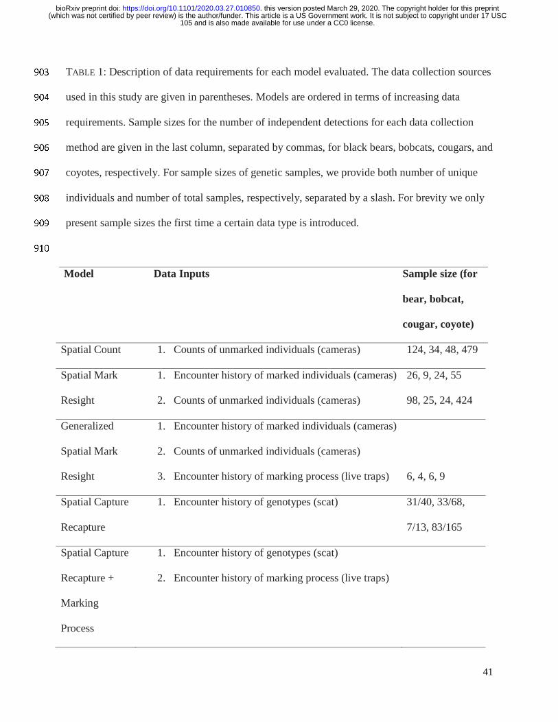
41

TABLE 1: Description of data requirements for each model evaluated. The data collection sources 903

used in this study are given in parentheses. Models are ordered in terms of increasing data 904

requirements. Sample sizes for the number of independent detections for each data collection 905

method are given in the last column, separated by commas, for black bears, bobcats, cougars, and 906

coyotes, respectively. For sample sizes of genetic samples, we provide both number of unique 907

individuals and number of total samples, respectively, separated by a slash. For brevity we only 908

present sample sizes the first time a certain data type is introduced. 909

910

Model Data Inputs Sample size (for

bear, bobcat,

cougar, coyote)

Spatial Count 1. Counts of unmarked individuals (cameras) 124, 34, 48, 479

Spatial Mark

Resight

1. Encounter history of marked individuals (cameras)

2. Counts of unmarked individuals (cameras)

26, 9, 24, 55

98, 25, 24, 424

Generalized

Spatial Mark

Resight



3. Encounter history of marking process (live traps)

6, 4, 6, 9

Spatial Capture

Recapture

1. Encounter history of genotypes (scat)

31/40, 33/68,

7/13, 83/165

Spatial Capture

Recapture +

Marking

Process

1. Encounter history of genotypes (scat)




https://doi.org/10.1101/2020.03.27.010850

42

Generalized

Spatial Mark

Resight +

Spatial Capture

Recapture




4. Encounter history of genotypes (scats)

911

912



https://doi.org/10.1101/2020.03.27.010850

43

FIGURE LEGENDS 913

FIG. 1: The study area. The black polygon represents the Starkey Experimental Forest and Range 914

boundary, green points are camera locations, and blue lines are scat detection dog survey tracks. 915

916

FIG. 2: a) Immobilized coyote fit with GPS collar. Note the colored shrinkwrap around collar 917

banding and unique number aiding in individual identification when photographed on remote 918

cameras. b) GPS collar positions for coyotes (light green), cougars (blue), bobcats (purple), and 919

bears (red) during the time sampling was conducted. The red outline is the Starkey Experimental 920

Forest and Range boundary. c) Scat located by detection dogs subsequently analyzed for species 921

ID and genotyped to determine individual identity. d) A GPS-collared bear detected on remote 922

camera. The number on the collar belting and location of the ear tag permitted individual 923

identification of this animal. 924

925

FIG. 3: A schematic diagram describing the data inputs for each model evaluated in this study. 926

We note that without the inclusion of GPS collar data, σ and s are still estimable but lack the 927

resolution provided by including telemetry data. 928

929

FIG. 4: Split violin plots displaying posterior distributions for the densities of bears, bobcats, 930

cougars, and coyotes across a suite of modeling methods. Within each panel, models are ordered 931

in terms of increasing data requirements with the most data-hungry models on the right. For each 932

model type, the left (blue) half of the violin excludes GPS telemetry data and the right (tan) half 933

includes GPS data. The white boxes display the 95% highest posterior density interval, and the 934

middle black bar indicates the posterior mode. Densities are presented as number of animals per 935



https://doi.org/10.1101/2020.03.27.010850

44

100 km2. Note that the spatial count models for each species required a different y-axis scale 936

than the other model types. 937

938

FIG. 5: Coefficients of variation for density estimates for bears, bobcats, cougars, and coyotes 939

(top left, clockwise). For each model type, the left (blue) bar excludes GPS data and the right 940

(tan) bar includes GPS data. The coefficient of variation was calculated as the standard deviation 941

divided by the posterior mean. Note that the sample size for the cougar SCR models was small (n 942

= 13 scats) and likely caused the relative imprecision for those models. 943

944

FIG. 6: Percent difference in the posterior mode of animal density compared to the SCR+GPS 945

model for black bears, bobcats, cougars, and coyotes. Note that the spatial count models for each 946

species required a different y-axis scale than the other model types. The dotted red line refers to 947

no difference from the SCR+GPS model; bars above the line indicate positive bias and bars 948

below the line indicate negative bias with respect to the SCR+GPS model. 949

950

FIG. 7: Violin plot showing SMR and SCR density estimates for coyotes modeled with and 951

without behavioral status (i.e. resident or transient). The left two violins show estimates from the 952

standard models while the right two display estimates from the model where sigma and detection 953

rates are allowed to vary as a function of behavioral status. 954

955



https://doi.org/10.1101/2020.03.27.010850

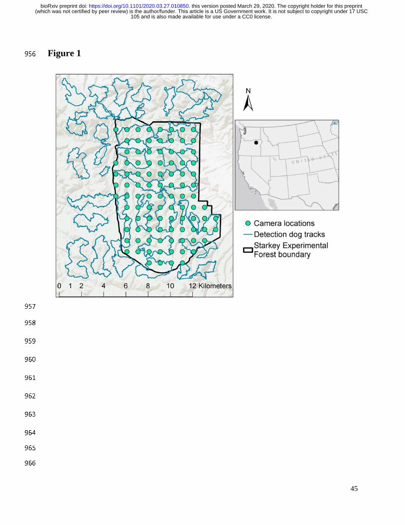
45

Figure 1 956

957

958

959

960

961

962

963

964

965

966



https://doi.org/10.1101/2020.03.27.010850

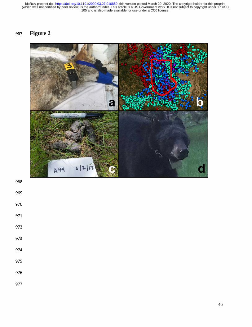
46

Figure 2 967

968

969

970

971

972

973

974

975

976

977

46



https://doi.org/10.1101/2020.03.27.010850

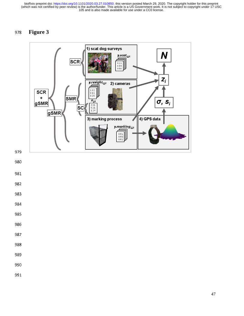
47

Figure 3 978

979

980

981

982

983

984

985

986

987

988

989

990

991



https://doi.org/10.1101/2020.03.27.010850

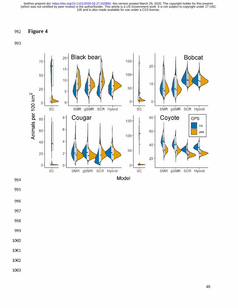
48

Figure 4 992

993

994

995

996

997

998

999

1000

1001

1002

1003



https://doi.org/10.1101/2020.03.27.010850

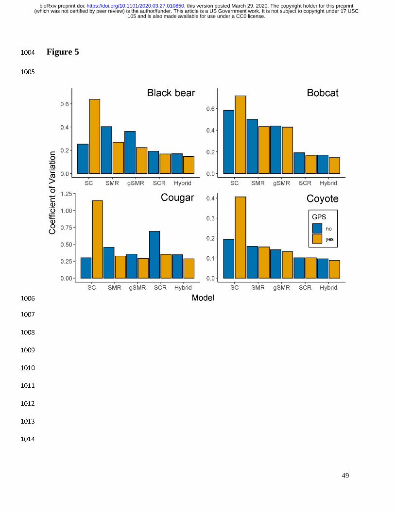
49

Figure 5 1004

1005

1006

1007

1008

1009

1010

1011

1012

1013

1014



https://doi.org/10.1101/2020.03.27.010850

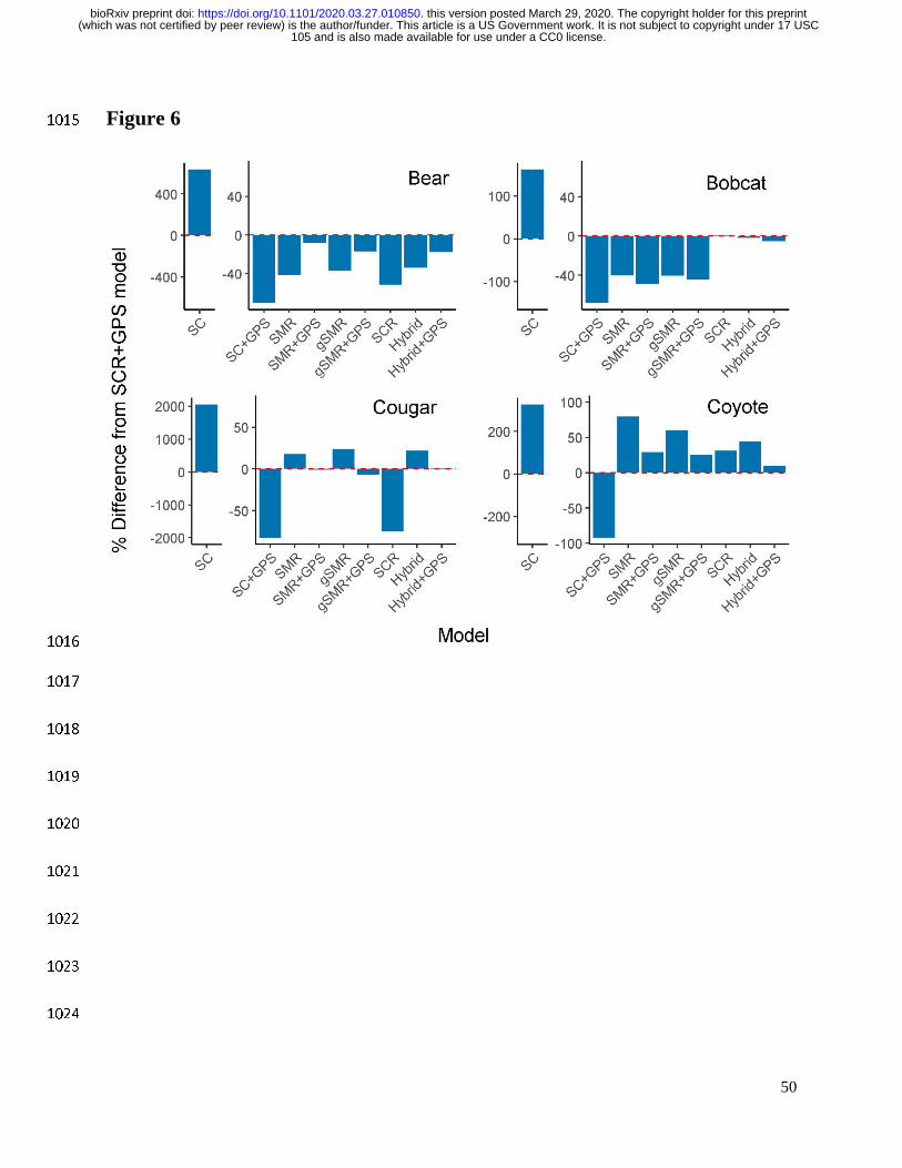
50

Figure 6 1015

1016

1017

1018

1019

1020

1021

1022

1023

1024



https://doi.org/10.1101/2020.03.27.010850

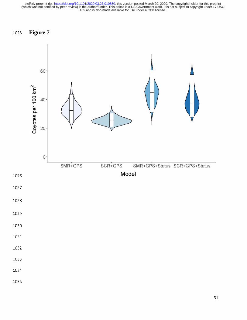
51

Figure 7 1025

1026

1027

1028

1029

1030

1031

1032

1033

1034

1035



https://doi.org/10.1101/2020.03.27.010850

Documents

Integrating spatial capture-recapture models with variable ... · density estimation, mark resight, noninvasive genetic sampling, spatial capture recapture a CC0 license. author/funder