Embed Size (px)
Citation preview
Bayesian Core:A Practical Approach to Computational Bayesian Statistics
Capture-recapture experiments
Capture-recapture experiments
4 Capture-recapture experimentsInference in finite populationsBinomial capture modelTwo-stage capture-recaptureOpen populationAccept-Reject methodsArnason–Schwarz’s Model
236 / 459

Bayesian Core:A Practical Approach to Computational Bayesian Statistics
Capture-recapture experiments
Inference in finite populations
Inference in finite populations
Problem of estimating an unknown population size, N , based onpartial observation of this population: domain of survey sampling
Warning
We do not cover the official Statistics/stratified type of surveybased on a preliminary knowledge of the structure of the population
237 / 459

Bayesian Core:A Practical Approach to Computational Bayesian Statistics
Capture-recapture experiments
Inference in finite populations
Numerous applications
Biology & Ecology for estimating the size of herds, of fish orwhale populations, etc.
Sociology & Demography for estimating the size ofpopulations at risk, including homeless people, prostitutes,illegal migrants, drug addicts, etc.
official Statistics in the U.S. and French census undercountprocedures
Economics & Finance in credit scoring, defaulting companies,etc.,
Fraud detection phone, credit card, etc.
Document authentication historical documents, forgery, etc.,
Software debugging
238 / 459

Bayesian Core:A Practical Approach to Computational Bayesian Statistics
Capture-recapture experiments
Inference in finite populations
Setup
Size N of the whole population is unknown but samples (withfixed or random sizes) can be extracted from the population.
239 / 459
Bayesian Core:A Practical Approach to Computational Bayesian Statistics
Capture-recapture experiments
Binomial capture model
The binomial capture model
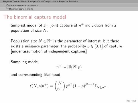
Simplest model of all: joint capture of n+ individuals from apopulation of size N .
Population size N ∈ N∗ is the parameter of interest, but there
exists a nuisance parameter, the probability p ∈ [0, 1] of capture[under assumption of independent captures]
Sampling modeln+ ∼ B(N, p)
and corresponding likelihood
ℓ(N, p|n+) =
(N
n+
)pn+
(1− p)N−n+IN≥n+ .
240 / 459
Bayesian Core:A Practical Approach to Computational Bayesian Statistics
Capture-recapture experiments
Binomial capture model
Bayesian inference (1)
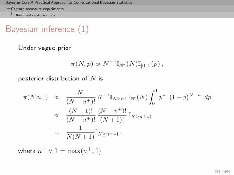
Under vague prior
π(N, p) ∝ N−1IN∗(N)I[0,1](p) ,
posterior distribution of N is
π(N |n+) ∝ N !
(N − n+)!N−1
IN≥n+IN∗(N)
∫ 1
0
pn+
(1− p)N−n+
dp
∝ (N − 1)!
(N − n+)!
(N − n+)!
(N + 1)!IN≥n+∨1
=1
N(N + 1)IN≥n+∨1 .
where n+ ∨ 1 = max(n+, 1)
241 / 459
Bayesian Core:A Practical Approach to Computational Bayesian Statistics
Capture-recapture experiments
Binomial capture model
Bayesian inference (2)
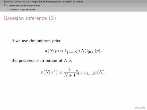
If we use the uniform prior
π(N, p) ∝ I{1,...,S}(N)I[0,1](p) ,
the posterior distribution of N is
π(N |n+) ∝ 1
N + 1I{n+∨1,...,S}(N) .
242 / 459

Bayesian Core:A Practical Approach to Computational Bayesian Statistics
Capture-recapture experiments
Binomial capture model
Capture-recapture data
European dippers
Birds closely dependent on streams,feeding on underwater invertebratesCapture-recapture data on dippersover years 1981–1987 in 3 zone of200 km2 in eastern France withmarkings and recaptures of breedingadults each year, during the breedingperiod from early March to earlyJune.
243 / 459
Bayesian Core:A Practical Approach to Computational Bayesian Statistics
Capture-recapture experiments
Binomial capture model
eurodip
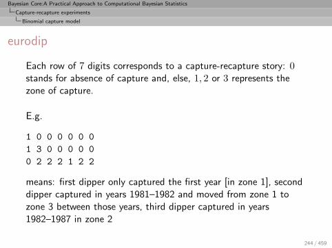
Each row of 7 digits corresponds to a capture-recapture story: 0stands for absence of capture and, else, 1, 2 or 3 represents thezone of capture.
E.g.
1 0 0 0 0 0 0
1 3 0 0 0 0 0
0 2 2 2 1 2 2
means: first dipper only captured the first year [in zone 1], seconddipper captured in years 1981–1982 and moved from zone 1 tozone 3 between those years, third dipper captured in years1982–1987 in zone 2
244 / 459

Bayesian Core:A Practical Approach to Computational Bayesian Statistics
Capture-recapture experiments
Two-stage capture-recapture
The two-stage capture-recapture experiment
Extension to the above with two capture periods plus a markingstage:
1 n1 individuals from a population of size N captured [sampledwithout replacement]
2 captured individuals marked and released
3 n2 individuals captured during second identical samplingexperiment
4 m2 individuals out of the n2’s bear the identification mark[captured twice]
245 / 459
Bayesian Core:A Practical Approach to Computational Bayesian Statistics
Capture-recapture experiments
Two-stage capture-recapture
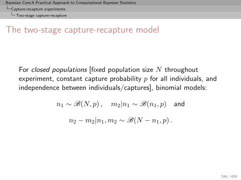
The two-stage capture-recapture model
For closed populations [fixed population size N throughoutexperiment, constant capture probability p for all individuals, andindependence between individuals/captures], binomial models:
n1 ∼ B(N, p) , m2|n1 ∼ B(n1, p) and
n2 −m2|n1,m2 ∼ B(N − n1, p) .
246 / 459
Bayesian Core:A Practical Approach to Computational Bayesian Statistics
Capture-recapture experiments
Two-stage capture-recapture
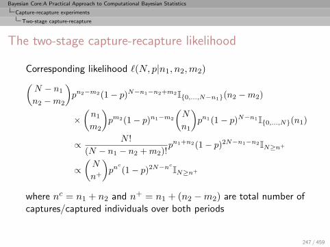
The two-stage capture-recapture likelihood
Corresponding likelihood ℓ(N, p|n1, n2,m2)
(N − n1
n2 −m2
)pn2−m2(1− p)N−n1−n2+m2I{0,...,N−n1}(n2 −m2)
×(n1
m2
)pm2(1− p)n1−m2
(N
n1
)pn1(1− p)N−n1I{0,...,N}(n1)
∝ N !
(N − n1 − n2 +m2)!pn1+n2(1− p)2N−n1−n2IN≥n+
∝(N
n+
)pnc
(1− p)2N−nc
IN≥n+
where nc = n1 + n2 and n+ = n1 + (n2 −m2) are total number ofcaptures/captured individuals over both periods
247 / 459
Bayesian Core:A Practical Approach to Computational Bayesian Statistics
Capture-recapture experiments
Two-stage capture-recapture
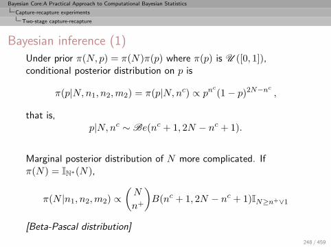
Bayesian inference (1)
Under prior π(N, p) = π(N)π(p) where π(p) is U ([0, 1]),conditional posterior distribution on p is
π(p|N,n1, n2,m2) = π(p|N,nc) ∝ pnc(1− p)2N−nc
,
that is,p|N,nc ∼ Be(nc + 1, 2N − nc + 1).
Marginal posterior distribution of N more complicated. Ifπ(N) = IN∗(N),
π(N |n1, n2,m2) ∝(N
n+
)B(nc + 1, 2N − nc + 1)IN≥n+∨1
[Beta-Pascal distribution]
248 / 459

Bayesian Core:A Practical Approach to Computational Bayesian Statistics
Capture-recapture experiments
Two-stage capture-recapture
Bayesian inference (2)Same problem if π(N) = N−1
IN∗(N).
Computations
Since N ∈ N, always possible to approximate the missingnormalizing factor in π(N |n1, n2,m2) by summing in N .Approximation errors become a problem when N and n+ are large.
Under proper uniform prior,
π(N) ∝ I{1,...,S}(N) ,
posterior distribution of N proportional to
π(N |n+) ∝(N
n+
)Γ(2N − nc + 1)
Γ(2N + 2)I{n+∨1,...,S}(N) .
and can be computed with no approximation error.249 / 459

Bayesian Core:A Practical Approach to Computational Bayesian Statistics
Capture-recapture experiments
Two-stage capture-recapture
The Darroch model
Simpler version of the above: conditional on both samples sizes n1
and n2,m2|n1, n2 ∼ H (N,n2, n1/N) .
Under uniform prior on N ∼ U ({1, . . . , S}), posterior distributionof N
π(N |m2) ∝(n1
m2
)(N − n1
n2 −m2
)/(N
n2
)I{n+∨1,...,S}(N)
and posterior expectations computed numerically by simplesummations.
250 / 459
Bayesian Core:A Practical Approach to Computational Bayesian Statistics
Capture-recapture experiments
Two-stage capture-recapture
eurodip
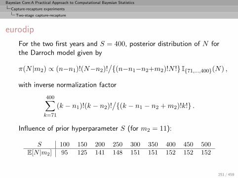
For the two first years and S = 400, posterior distribution of N forthe Darroch model given by
π(N |m2) ∝ (n−n1)!(N−n2)!/{(n−n1−n2+m2)!N !} I{71,...,400}(N) ,
with inverse normalization factor
400∑
k=71
(k − n1)!(k − n2)!/{(k − n1 − n2 +m2)!k!} .
Influence of prior hyperparameter S (for m2 = 11):
S 100 150 200 250 300 350 400 450 500E[N |m2] 95 125 141 148 151 151 152 152 152
251 / 459

Bayesian Core:A Practical Approach to Computational Bayesian Statistics
Capture-recapture experiments
Two-stage capture-recapture
Gibbs sampler for 2-stage capture-recapture
If n+ > 0, both conditional posterior distributions are standard,since
p|nc, N ∼ Be(nc + 1, 2N − nc + 1)
N − n+|n+, p ∼ N eg(n+, 1− (1− p)2) .
Therefore, joint distribution of (N, p) can be approximated by aGibbs sampler
252 / 459

Bayesian Core:A Practical Approach to Computational Bayesian Statistics
Capture-recapture experiments
Two-stage capture-recapture
T -stage capture-recapture modelFurther extension to the two-stage capture-recapture model: seriesof T consecutive captures.nt individuals captured at period 1 ≤ t ≤ T , and mt recapturedindividuals (with the convention that m1 = 0)
n1 ∼ B(N, p)
and, conditional on earlier captures/recaptures (2 ≤ j ≤ T ),
mj ∼ B
(j−1∑
t=1
(nt −mt), p
)and
nj −mj ∼ B
(N −
j−1∑
t=1
(nt −mt), p
).
253 / 459

Bayesian Core:A Practical Approach to Computational Bayesian Statistics
Capture-recapture experiments
Two-stage capture-recapture
T -stage capture-recapture likelihood
Likelihood ℓ(N, p|n1, n2,m2 . . . , nT ,mT ) given by
(N
n1
)pn1(1− p)N−n1
T∏
j=2
[(N −∑j−1
t=1 (nt −mt)
nj −mj
)pnj−mj
× (1− p)N−Pj
t=1(nt−mt)
(∑j−1t=1 (nt −mt)
mj
)
× pmj (1− p)Pj−1
t=1 (nt−mt)−mj
].
254 / 459

Bayesian Core:A Practical Approach to Computational Bayesian Statistics
Capture-recapture experiments
Two-stage capture-recapture
Sufficient statistics
Simplifies into
ℓ(N, p|n1, n2,m2 . . . , nT ,mT ) ∝ N !
(N − n+)!pnc
(1−p)TN−ncIN≥n+
with the sufficient statistics
n+ =T∑
t=1
(nt −mt) and nc =T∑
t=1
nt ,
total number of captured individuals/captures over the T periods
255 / 459

Bayesian Core:A Practical Approach to Computational Bayesian Statistics
Capture-recapture experiments
Two-stage capture-recapture
Bayesian inference (1)
Under noninformative prior π(N, p) = 1/N , joint posterior
π(N, p|n+, nc) ∝ (N − 1)!
(N − n+)!pnc
(1− p)TN−nc
IN≥n+∨1 .
leads to conditional posterior
p|N,n+, nc ∼ Be(nc + 1, TN − nc + 1)
and marginal posterior
π(N |n+, nc) ∝ (N − 1)!
(N − n+)!
(TN − nc)!
(TN + 1)!IN≥n+∨1
which is computable [under previous provisions].
Alternative Gibbs sampler also available.
256 / 459
Bayesian Core:A Practical Approach to Computational Bayesian Statistics
Capture-recapture experiments
Two-stage capture-recapture
Bayesian inference (2)
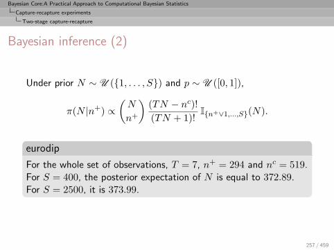
Under prior N ∼ U ({1, . . . , S}) and p ∼ U ([0, 1]),
π(N |n+) ∝(N
n+
)(TN − nc)!
(TN + 1)!I{n+∨1,...,S}(N).
eurodip
For the whole set of observations, T = 7, n+ = 294 and nc = 519.For S = 400, the posterior expectation of N is equal to 372.89.For S = 2500, it is 373.99.
257 / 459

Bayesian Core:A Practical Approach to Computational Bayesian Statistics
Capture-recapture experiments
Two-stage capture-recapture
Computational difficulties
E.g., heterogeneous capture–recapture model where individuals arecaptured at time 1 ≤ t ≤ T with probability pt with both N andthe pt’s are unknown.
Corresponding likelihood
ℓ(N, p1, . . . , pT |n1, n2,m2 . . . , nT ,mT )
∝ N !
(N − n+)!
T∏
t=1
pntt (1− pt)
N−nt .
258 / 459
Bayesian Core:A Practical Approach to Computational Bayesian Statistics
Capture-recapture experiments
Two-stage capture-recapture
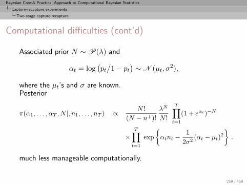
Computational difficulties (cont’d)
Associated prior N ∼ P(λ) and
αt = log(pt
/1− pt
)∼ N (µt, σ
2),
where the µt’s and σ are known.Posterior
π(α1, . . . , αT , N |, n1, . . . , nT ) ∝ N !
(N − n+)!
λN
N !
T∏
t=1
(1 + eαt)−N
×T∏
t=1
exp
{αtnt −
1
2σ2(αt − µt)
2
}.
much less manageable computationally.
259 / 459

Bayesian Core:A Practical Approach to Computational Bayesian Statistics
Capture-recapture experiments
Open population
Open populations
More realistically, population size does not remain fixed over time:probability q for each individual to leave the population at eachtime [or between each capture episode]
First occurrence of missing variable model.
Simplified version where only individuals captured during the firstexperiment are marked and their subsequent recaptures areregistered.
260 / 459
Bayesian Core:A Practical Approach to Computational Bayesian Statistics
Capture-recapture experiments
Open population
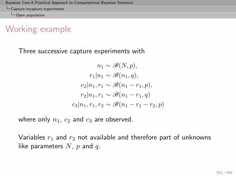
Working example
Three successive capture experiments with
n1 ∼ B(N, p),
r1|n1 ∼ B(n1, q),
c2|n1, r1 ∼ B(n1 − r1, p),
r2|n1, r1 ∼ B(n1 − r1, q)
c3|n1, r1, r2 ∼ B(n1 − r1 − r2, p)
where only n1, c2 and c3 are observed.
Variables r1 and r2 not available and therefore part of unknownslike parameters N , p and q.
261 / 459

Bayesian Core:A Practical Approach to Computational Bayesian Statistics
Capture-recapture experiments
Open population
Bayesian inference
Likelihood(N
n1
)pn1(1− p)N−n1
(n1
r1
)qr1(1− q)n1−r1
(n1 − r1c2
)pc2(1− p)n1−r1−c2
(n1 − r1r2
)qr2(1− q)n1−r1−r2
(n1 − r1 − r2
c3
)pc3(1− p)n1−r1−r2−c3
and priorπ(N, p, q) = N−1
I[0,1](p)I[0,1](q)
262 / 459

Bayesian Core:A Practical Approach to Computational Bayesian Statistics
Capture-recapture experiments
Open population
Full conditionals for Gibbs sampling
π(p|N, q,D∗) ∝ pn+(1− p)u+
π(q|N, p,D∗) ∝ qc1+c2(1− q)2n1−2r1−r2
π(N |p, q,D∗) ∝ (N − 1)!
(N − n1)!(1− p)N
IN≥n1
π(r1|p, q, n1, c2, c3, r2) ∝(n1 − r1)! q
r1(1− q)−2r1(1− p)−2r1
r1!(n1 − r1 − r2 − c3)!(n1 − c2 − r1)!
π(r2|p, q, n1, c2, c3, r1) ∝qr2 [(1− p)(1− q)]−r2
r2!(n1 − r1 − r2 − c3)!
where
D∗ = (n1, c2, c3, r1, r2)
u1 = N − n1, u2 = n1 − r1 − c2, u3 = n1 − r1 − r2 − c3
n+ = n1 + c2 + c3, u+ = u1 + u2 + u3
263 / 459
Bayesian Core:A Practical Approach to Computational Bayesian Statistics
Capture-recapture experiments
Open population
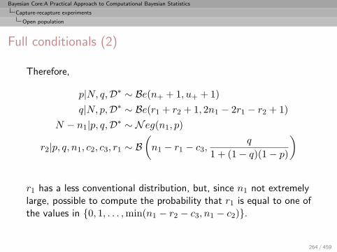
Full conditionals (2)
Therefore,
p|N, q,D∗ ∼ Be(n+ + 1, u+ + 1)
q|N, p,D∗ ∼ Be(r1 + r2 + 1, 2n1 − 2r1 − r2 + 1)
N − n1|p, q,D∗ ∼ N eg(n1, p)
r2|p, q, n1, c2, c3, r1 ∼ B(n1 − r1 − c3,
q
1 + (1− q)(1− p)
)
r1 has a less conventional distribution, but, since n1 not extremelylarge, possible to compute the probability that r1 is equal to one ofthe values in {0, 1, . . . ,min(n1 − r2 − c3, n1 − c2)}.
264 / 459
Bayesian Core:A Practical Approach to Computational Bayesian Statistics
Capture-recapture experiments
Open population
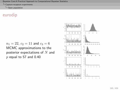
eurodip
n1 = 22, c2 = 11 and c3 = 6MCMC approximations to theposterior expectations of N andp equal to 57 and 0.40
0 2000 4000 6000 8000 10000
0.0
0.2
0.4
0.6
p
0.0 0.2 0.4 0.6
01
23
45
0 2000 4000 6000 8000 10000
0.0
00
.10
0.2
0
q
0.00 0.05 0.10 0.15 0.20 0.25 0.30 0.35
05
15
25
0 2000 4000 6000 8000 10000
50
10
02
00
N
50 100 150 200
0.0
00
0.0
15
0.0
30
0 2000 4000 6000 8000 10000
02
46
81
0
r 1
0 2 4 6 8 10
02
46
8
0 2000 4000 6000 8000 10000
01
23
45
6
r 2
0 2 4 6 8
02
46
265 / 459

Bayesian Core:A Practical Approach to Computational Bayesian Statistics
Capture-recapture experiments
Open population
eurodip
n1 = 22, c2 = 11 and c3 = 6MCMC approximations to theposterior expectations of N andp equal to 57 and 0.40
0 1 2 3 4 5
01
23
45
6
r1
r 2
266 / 459

Bayesian Core:A Practical Approach to Computational Bayesian Statistics
Capture-recapture experiments
Accept-Reject methods
Accept-Reject methods
Many distributions from which it is difficult, or evenimpossible, to directly simulate.
Technique that only require us to know the functional form ofthe target π of interest up to a multiplicative constant.
Key to this method is to use a proposal density g [as inMetropolis-Hastings]
267 / 459

Bayesian Core:A Practical Approach to Computational Bayesian Statistics
Capture-recapture experiments
Accept-Reject methods
Principle
Given a target density π, find a density g and a constant M suchthat
π(x) ≤Mg(x)
on the support of π.
Accept-Reject algorithm is then
1 Generate X ∼ g, U ∼ U[0,1] ;
2 Accept Y = X if U ≤ f(X)Mg(X) ;
3 Return to 1. otherwise.
268 / 459

Bayesian Core:A Practical Approach to Computational Bayesian Statistics
Capture-recapture experiments
Accept-Reject methods
Validation of Accept-Reject
This algorithm produces a variable Ydistributed according to f
Fundamental theorem of simulation
SimulatingX ∼ f(x)
is equivalent to simulating
(X,U) ∼ U{(x, u) : 0 < u < π(x)} −2 0 2 4 6 8 10 120
0.05
0.1
0.15
0.2
0.25
0.3
0.35
269 / 459

Bayesian Core:A Practical Approach to Computational Bayesian Statistics
Capture-recapture experiments
Accept-Reject methods
Two interesting properties:
◦ First, Accept-Reject provides a generic method to simulatefrom any density π that is known up to a multiplicative factorParticularly important for Bayesian calculations since
π(θ|x) ∝ π(θ) f(x|θ) .
is specified up to a normalizing constant
◦ Second, the probability of acceptance in the algorithm is1/M , e.g., expected number of trials until a variable isaccepted is M
270 / 459
Bayesian Core:A Practical Approach to Computational Bayesian Statistics
Capture-recapture experiments
Accept-Reject methods
Application to the open population model
Since full conditional distribution of r1 non-standard, rather thanusing exhaustive enumeration of all probabilitiesP(m1 = k) = π(k) and then sampling from this distribution, try touse a proposal based on a binomial upper bound.
Take g equal to the binomial B(n1, q1) with
q1 = q/(1− q)2(1− p)2
271 / 459

Bayesian Core:A Practical Approach to Computational Bayesian Statistics
Capture-recapture experiments
Accept-Reject methods
Proposal bound
π(k)/g(k) proportional to`
n1−c2k
´(1− q1)
k`
n1−kr2+c3
´`
n1k
´ =(n1 − c2)!
(r2 + c3)!n1!
((n1 − k)!)2(1− q1)k
(n1 − c2 − k)!(n1 − r2 − c3 − k)!
decreasing in k, therefore bounded by
(n1 − c2)!
(r2 + c3)!
n1!
(n1 − c2)!(n1 − r2 − c3)!=
(n1
r2 + c3
).
This is not the constant M because of unnormalised densities[M may also depend on q1]. Therefore the averageacceptance rate is undetermined and requires an extra MonteCarlo experiment
272 / 459
Bayesian Core:A Practical Approach to Computational Bayesian Statistics
Capture-recapture experiments
Arnason–Schwarz’s Model
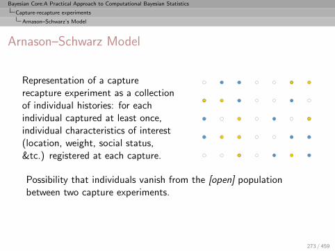
Arnason–Schwarz Model
Representation of a capturerecapture experiment as a collectionof individual histories: for eachindividual captured at least once,individual characteristics of interest(location, weight, social status,&tc.) registered at each capture.
Possibility that individuals vanish from the [open] populationbetween two capture experiments.
273 / 459
Bayesian Core:A Practical Approach to Computational Bayesian Statistics
Capture-recapture experiments
Arnason–Schwarz’s Model
Parameters of interest
Study the movements of individuals between zones/strata ratherthan estimating population size.
Two types of variables associated with each individual i = 1, . . . , n
1 a variable for its location [partly observed],
zi = (z(i,t), t = 1, .., τ)
where τ is the number of capture periods,
2 a binary variable for its capture history [completely observed],
xi = (x(i,t), t = 1, .., τ) .
274 / 459

Bayesian Core:A Practical Approach to Computational Bayesian Statistics
Capture-recapture experiments
Arnason–Schwarz’s Model
Migration & deaths
z(i,t) = r when individual i is alive in stratum r at time t anddenote z(i,t) = † for the case when it is dead at time t.
Variable zi sometimes called migration process of individual i aswhen animals moving between geographical zones.
E.g.,
xi = 1 1 0 1 1 1 0 0 0 and zi = 1 2 · 3 1 1 · · ·
for which a possible completed zi is
zi = 1 2 1 3 1 1 2 † †
meaning that animal died between 7th and 8th captures
275 / 459
Bayesian Core:A Practical Approach to Computational Bayesian Statistics
Capture-recapture experiments
Arnason–Schwarz’s Model
No tag recovery
We assume that
† is absorbing
z(i,t) = † always corresponds to x(i,t) = 0.
the (xi, zi)’s (i = 1, . . . , n) are independent
each vector zi is a Markov chain on K ∪ {†} with uniforminitial probability on K.
276 / 459
Bayesian Core:A Practical Approach to Computational Bayesian Statistics
Capture-recapture experiments
Arnason–Schwarz’s Model
Reparameterisation
Parameters of the Arnason–Schwarz model are
1 capture probabilities
pt(r) = P(x(i,t) = 1|z(i,t) = r
)
2 transition probabilities
qt(r, s) = P(z(i,t+1) = s|z(i,t) = r
)r ∈ K, s ∈ K∪{†}, qt(†, †) = 1
3 survival probabilities φt(r) = 1− qt(r, †)4 inter-strata movement probabilities ψt(r, s) such that
qt(r, s) = φt(r)× ψt(r, s) r ∈ K, s ∈ K .
277 / 459

Bayesian Core:A Practical Approach to Computational Bayesian Statistics
Capture-recapture experiments
Arnason–Schwarz’s Model
Modelling
Likelihood
ℓ((x1, z1), . . . , (xn, zn)) ∝n∏
i=1
[τ∏
t=1
pt(z(i,t))x(i,t)(1− pt(z(i,t)))
1−x(i,t)×
τ−1∏
t=1
qt(z(i,t), z(i,t+1))
].
278 / 459
Bayesian Core:A Practical Approach to Computational Bayesian Statistics
Capture-recapture experiments
Arnason–Schwarz’s Model
Conjugate priors
Capture and survival parameters
pt(r) ∼ Be(at(r), bt(r)) , φt(r) ∼ Be(αt(r), βt(r)) ,
where at(r), . . . depend on both time t and location r,For movement probabilities/Markov transitionsψt(r) = (ψt(r, s); s ∈ K),
ψt(r) ∼ Dir(γt(r)) ,
since ∑
s∈K
ψt(r, s) = 1 ,
where γt(r) = (γt(r, s); s ∈ K).
279 / 459

Bayesian Core:A Practical Approach to Computational Bayesian Statistics
Capture-recapture experiments
Arnason–Schwarz’s Model
lizards
Capture–recapture experiment on the migrations of lizards betweenthree adjacent zones, with are six capture episodes.
Prior information provided by biologists on pt (which are assumedto be zone independent) and φt(r), in the format of priorexpectations and prior confidence intervals.
Differences in prior on pt due to differences in capture effortsdifferences between episodes 1, 3, 5 and 2, 4 due to differentmortality rates over winter.
280 / 459

Bayesian Core:A Practical Approach to Computational Bayesian Statistics
Capture-recapture experiments
Arnason–Schwarz’s Model
Prior information
Episode 2 3 4 5 6
pt Mean 0.3 0.4 0.5 0.2 0.295% int. [0.1,0.5] [0.2,0.6] [0.3,0.7] [0.05,0.4] [0.05,0.4]
Site A B,CEpisode t=1,3,5 t=2,4 t=1,3,5 t=2,4
φt(r) Mean 0.7 0.65 0.7 0.795% int. [0.4,0.95] [0.35,0.9] [0.4,0.95] [0.4,0.95]
281 / 459
Bayesian Core:A Practical Approach to Computational Bayesian Statistics
Capture-recapture experiments
Arnason–Schwarz’s Model
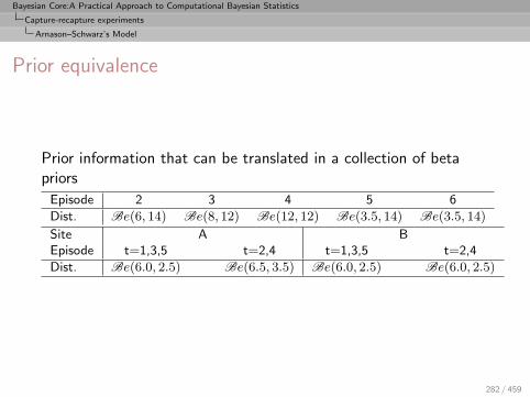
Prior equivalence
Prior information that can be translated in a collection of betapriors
Episode 2 3 4 5 6
Dist. Be(6, 14) Be(8, 12) Be(12, 12) Be(3.5, 14) Be(3.5, 14)
Site A BEpisode t=1,3,5 t=2,4 t=1,3,5 t=2,4
Dist. Be(6.0, 2.5) Be(6.5, 3.5) Be(6.0, 2.5) Be(6.0, 2.5)
282 / 459

Bayesian Core:A Practical Approach to Computational Bayesian Statistics
Capture-recapture experiments
Arnason–Schwarz’s Model
eurodip
Prior belief that the capture and survival rates should be constantover time
pt(r) = p(r) and φt(r) = φ(r)
Assuming in addition that movement probabilities aretime-independent,
ψt(r) = ψ(r)
we are left with 3[p(r)] + 3[φ(r)] + 3× 2[φt(r)] = 12 parameters.
Use non-informative priors with
a(r) = b(r) = α(r) = β(r) = γ(r, s) = 1
283 / 459

Bayesian Core:A Practical Approach to Computational Bayesian Statistics
Capture-recapture experiments
Arnason–Schwarz’s Model
Gibbs sampling
Needs to account for the missing parts in the zi’s, in order tosimulate the parameters from the full conditional distributions
π(θ|x, z) ∝ ℓ(θ|x, z)× π(θ) ,
where x and z are the collections of the vectors of captureindicators and locations.
Particular case of data augmentation, where the missing data z issimulated at each step t in order to reconstitute a complete sample(x, z(t)) with two steps:
Parameter simulation
Missing location simulation
284 / 459

Bayesian Core:A Practical Approach to Computational Bayesian Statistics
Capture-recapture experiments
Arnason–Schwarz’s Model
Arnason–Schwarz Gibbs sampler
Algorithm
Iteration l (l ≥ 1)
1 Parameter simulationsimulate θ(l) ∼ π(θ|z(l−1),x) as (t = 1, . . . , τ)
p(l)t (r)|x, z(l−1) ∼ Be
(at(r) + ut(r), bt(r) + v
(l)t (r)
)
φ(l)t (r)|x, z(l−1) ∼ Be
αt(r) +
∑
j∈K
w(l)t (r, j), βt(r) + w
(l)t (r, †)
ψ(l)t (r)|x, z(l−1) ∼ Dir
(γt(r, s) + w
(l)t (r, s); s ∈ K
)
285 / 459

Bayesian Core:A Practical Approach to Computational Bayesian Statistics
Capture-recapture experiments
Arnason–Schwarz’s Model
Arnason–Schwarz Gibbs sampler (cont’d)
where
w(l)t (r, s) =
n∑
i=1
I(z
(l−1)(i,t)
=r,z(l−1)(i,t+1)
=s)
u(l)t (r) =
n∑
i=1
I(x(i,t)=1,z
(l−1)(i,t)
=r)
v(l)t (r) =
n∑
i=1
I(x(i,t)=0,z
(l−1)(i,t)
=r)
286 / 459

Bayesian Core:A Practical Approach to Computational Bayesian Statistics
Capture-recapture experiments
Arnason–Schwarz’s Model
Arnason–Schwarz Gibbs sampler (cont’d)
2 Missing location simulation
generate the unobserved z(l)(i,t)’s from the full conditional
distributions
P(z(l)
(i,1) = s|x(i,1), z(l−1)
(i,2) , θ(l)) ∝ q(l)1 (s, z
(l−1)
(i,2) )(1− p(l)1 (s)) ,
P(z(l)
(i,t) = s|x(i,t), z(l)
(i,t−1), z(l−1)
(i,t+1), θ(l)) ∝ q
(l)t−1(z
(l)
(i,t−1), s)
× qt(s, z(l−1)
(i,t+1))(1− p(l)t (s)) ,
P(z(l)
(i,τ) = s|x(i,τ), z(l)
(i,τ−1), θ(l)) ∝ q
(l)τ−1(z
(l)
(i,τ−1), s)(1− pτ (s)(l)) .
287 / 459

Bayesian Core:A Practical Approach to Computational Bayesian Statistics
Capture-recapture experiments
Arnason–Schwarz’s Model
Gibbs sampler illustrated
Take K = {1, 2}, n = 4, m = 8 and ,for x,
1 1 1 · · 1 · · ·2 1 · 1 · 1 · 2 13 2 1 · 1 2 · · 14 1 · · 1 2 1 1 2
Take all hyperparameters equal to 1
288 / 459
Bayesian Core:A Practical Approach to Computational Bayesian Statistics
Capture-recapture experiments
Arnason–Schwarz’s Model
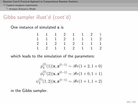
Gibbs sampler illust’d (cont’d)
One instance of simulated z is
1 1 1 2 1 1 2 †1 1 1 2 1 1 1 22 1 2 1 2 1 1 11 2 1 1 2 1 1 2
which leads to the simulation of the parameters:
p(l)4 (1)|x, z(l−1) ∼ Be(1 + 2, 1 + 0)
φ(l)7 (2)|x, z(l−1) ∼ Be(1 + 0, 1 + 1)
ψ(l)2 (1, 2)|x, z(l−1) ∼ Be(1 + 1, 1 + 2)
in the Gibbs sampler.
289 / 459

Bayesian Core:A Practical Approach to Computational Bayesian Statistics
Capture-recapture experiments
Arnason–Schwarz’s Model
eurodip
Fast convergence
0 2000 4000 6000 8000 10000
0.20
0.25
0.30
0.35
p(1)
0.15 0.20 0.25 0.30 0.35 0.40
05
1015
0 2000 4000 6000 8000 10000
0.96
0.97
0.98
0.99
1.00
φ(2)
0.94 0.95 0.96 0.97 0.98 0.99 1.00
020
4060
8010
0
0 2000 4000 6000 8000 10000
0.45
0.55
0.65
0.75
ψ(3, 3)
0.4 0.5 0.6 0.7
02
46
8
290 / 459